exogenous vs. endogenous separation · exogenous vs. endogenous separation garey ramey december...

Exogenous vs. Endogenous Separation

Garey Ramey�

December 2007

Revised August 2008

Abstract

This paper assesses how various approaches to modelling the separation

margin a¤ect the ability of the Mortensen-Pissarides job matching model to

explain key facts about the aggregate labor market. Allowing for realistic time

variation in the separation rate, whether exogenous or endogenous, greatly in-

creases the unemployment variability generated by the model. Speci�cations

with exogenous separation rates, whether constant or time-varying, fail to pro-

duce realistic volatility and productivity responsiveness of the separation rate

and worker �ows. Speci�cations with endogenous separation rates, on the other

hand, succeed along these dimensions. In addition, the endogenous separation

model with on-the-job search yields a realistic Beveridge curve correlation, and

it performs well in accounting for the productivity responsiveness of vacancies

and market tightness. When the Hagedorn-Manovskii calibration approach

is used, the behavior of the job �nding rate, vacancies and market tightness

becomes more realistic, but the approach yields only a negligible volume of

job-to-job transitions in the on-the-job search speci�cation.

�University of California San Diego. Email: [email protected]. Web page: http://www.econ.ucsd.edu/

~gramey. I would like to thank Wouter Den Haan, Shigeru Fujita, Bob Hall, Guiseppe Moscarini, Dale

Mortensen, Mike Owyang, Chris Pissarides, Valerie Ramey, and seminar participants at the Federal Reserve

Bank of Philadelphia, the 2008 Midwest Macro Meetings and the 2008 Meeting of the SED for helpful

comments and conversations.

1

1 Introduction

In its complete form, the Mortensen-Pissarides job matching model (henceforth MP model)

endogenously determines both the match creation and separation margins.1 While re-

searchers agree that match creation is appropriately viewed as endogenous, there is little

consensus as to the proper treatment of the separation margin. Papers such as Cole and

Rogerson (1999), Fujita (2003, 2004), Mortensen and Nagypál (2007b), Mortensen and

Pissarides (1994), Pissarides (2007) and others allow match dissolution to be responsive

to incentives facing the worker and �rm. On the other hand, Costain and Reiter (2006),

Fujita and Ramey (2007), Hagedorn and Manovskii (2008), Hall (2005), Hornstein, et al.

(2006), Mortensen and Nagypál (2007a), Shimer (2005), Yashiv (2006) and others specify

that matches break up at a rate that is exogenous and constant, a¤ected by neither in-

centives nor cyclical factors. Mortensen (2005), Mortensen and Nagypál (2007a), Shimer

(2005) and Yashiv (2006) consider a third possibility, namely that separation rates vary

over time in a random manner, while Krause and Lubik (2006), Mortensen (1994, 2005),

Nagypál (2005a,b), Pissarides (1994), Tasci (2006) and others allow for separation directly

to new jobs.

This paper assesses how these various approaches to modeling the separation margin

a¤ect the ability of the MP model to explain key facts about unemployment, transition

rates, worker �ows and other variables. A discrete-time version of Pissarides�(2000) speci-

�cation is calibrated at weekly frequency. Match separation is parameterized in four ways:

(i) constant separation rate; (ii) exogenous separation rate following an AR(1) process;

(iii) endogenous separation rate without on-the-job search (OJS); and (iv) endogenous

separation rate with OJS. For the two speci�cations with endogenous separation, match-

speci�c productivity factors follow a persistent stochastic process, i.e., the factors are not

required to be i.i.d. over time, as in many previous papers. The model is solved us-

ing a nonlinear method that parameterizes match surplus and market tightness (i.e., the

vacancy-unemployment ratio) on a grid, and iterates backward to exploit stability of the

backward dynamics.

In calibrating the model, the values of the workers�unemployment bene�t and bar-

gaining weight, as well as the elasticity parameter of the matching function, are set to

standard values advocated by Mortensen and Nagypál (2007a). The calibration of the

1Throughout this paper, the terms �separation�and �job �nding�denote movements of workers between

employed and unemployed status.

2

vacancy posting cost draws on survey evidence from Barron and Bishop (1985) and Bar-

ron, et al. (1997). Other parameters are chosen to match the mean monthly job �nding

and separation rates calculated by Fujita and Ramey (2006), who consider data from the

Current Population Survey (CPS) over the 1976-2005 period. In addition, each of the

three speci�cations with time-varying separation rates is calibrated to match the standard

deviation of the separation rate observed in the Fujita-Ramey data. For the OJS speci-

�cation, the cost of OJS is calibrated by matching the average job-to-job transition rate

measured by Moscarini and Thomsson (2007) using CPS data.

Statistics calculated from simulated data for the four speci�cations are compared to

corresponding statistics obtained from the Fujita-Ramey data. The results show, �rst

of all, that the model with constant separation rates fares poorly in accounting for the

volatility of key labor market variables. It does not, of course, explain the substantial

variability of the separation rate observed in the data; nor does it generate anywhere near

the empirical volatility of unemployment, a point stressed by Costain and Reiter (2006) and

Shimer (2005). In addition, the variability of gross worker �ows, both unemployment-to-

employment (UE) and employment-to-unemployment (EU), is far too low in the constant

separation rate model.

On the other hand, the three speci�cations with time-varying separation rates, which

are calibrated to match the volatility of the empirical separation rate, each generate sub-

stantially greater volatility of unemployment and worker �ows. In the model with OJS,

for example, the standard deviation of unemployment equals 60 percent of its empirical

value. Moreover, the three speci�cations match closely the standard deviations of UE

and EU �ows. Introducing realistic variability at the separation margin thus substantially

improves the performance of the MP model in accounting for unemployment and worker

�ow variability.

In the data, the separation rate and the two worker �ow variables exhibit substantial

negative correlations with productivity.2 Both versions of the MP model with exogenous

separation fail along this dimension, as they generate essentially no productivity comove-

ment of separation rates and worker �ows. The two versions with endogenous separation,

however, exhibit realistic responsiveness of these variables to productivity. Endogeneity of

the separation rate appears central to explaining the cyclical properties of the separation

rate and worker �ows.2These negative correlations, obtained from CPS data, are corroborated by data from the Survey on

Income and Program Participation (SIPP); see Section 3.3 below.

3

The two endogenous separation speci�cations di¤er in their ability to account for the

Beveridge curve relationship, wherein unemployment and vacancies display strong nega-

tive correlation. In the absence of OJS, the model with endogenous separation produces a

counterfactually positive unemployment-vacancy correlation, due to fact that higher un-

employment makes workers easier to �nd during downturns, stimulating the posting of

vacancies. With OJS, however, downturns also imply a fall in the number of employed

searchers, militating against the rise in unemployment. The unemployment-vacancy cor-

relation becomes strongly negative in this case, matching closely the empirical value.

Endogenous separation is therefore consistent with the Beveridge curve relationship when

OJS is added to the model. Moreover, this speci�cation captures the negative correlation

between the job �nding and separation rates seen in the data.

In summary, the endogenous separation speci�cation with OJS implies empirically rea-

sonable volatility and productivity responsiveness of unemployment, the separation rate

and worker �ows, along with realistic Beveridge curve and transition rate correlations.

Each of the remaining three speci�cations fails decisively along one or more of these di-

mensions. This provides strong support for the OJS model as the most valid speci�cation.

The results also show, however, that the MP model under the standard calibration does

not produce realistic volatility of the job �nding rate, irrespective of how the separation

margin is modelled. The empirical standard deviation of the job �nding rate is nearly six

times the simulated value for each of the four speci�cations, and the comparison is similar

for the productivity elasticity. This failure to generate realistic behavior at the job �nding

margin, which lies at the heart of the Hall-Shimer critique of the MP model, is thus not

resolved by introducing realistic behavior at the separation margin.

The three speci�cations without OJS also deliver insu¢ cient productivity responsive-

ness of vacancies and market tightness. In the OJS speci�cation, however, these variables

are much more responsive to productivity: the productivity elasticities of vacancies and

market tightness in the simulated data amount to roughly 50 and 75 percent, respectively,

of their empirical values. In the OJS speci�cation, procyclical variation in the number

of searching workers makes vacancies more responsive to productivity at given levels of

market tightness.

The MP model is further evaluated in terms of its ability to generate realistic dynamic

interrelationships, as captured by cross correlations at various leads and lags. None of the

four speci�cations reproduces the sluggish productivity responses of unemployment, the

job �nding rate, vacancies and market tightness that are seen in the data. As pointed

4

out by Fujita and Ramey (2007), rapid adjustment of vacancies prevents the model from

exhibiting realistic dynamics with respect to these variables. The OJS speci�cation does,

however, demonstrate empirically reasonable dynamic patterns along the other dimensions

considered, including the cross correlations between unemployment and vacancies, and

between job �nding and separation rates.

Hagedorn and Manovskii (2008) propose an alternative calibration strategy, drawing

on empirical information on wages and pro�ts, that raises the volatility of unemployment,

market tightness and other variables in the constant separation rate model. To investigate

the robustness of the current �ndings to this alternative, the constant separation rate

and OJS speci�cations are suitably recalibrated. In line with Hagedorn and Manovskii�s

�ndings, this procedure yields much more realistic volatility of unemployment, the job

�nding rate, vacancies and market tightness. It does not, however, remedy the key failings

of the constant separation rate model: in particular, the separation rate and worker �ows

continue to display unrealistic variability and productivity comovement. Moreover, the

HM calibration implies a negligibly small job-to-job transition rate, even when the cost of

OJS is zero.

Numerous previous papers have evaluated the properties of the MP model in dynamic

stochastic equilibrium. Most closely related are Mortensen and Pissarides (1994) and

Mortensen (1994). These papers calibrate and simulate endogenous separation versions

of the standard MP model in continuous time, and stress the model�s ability to explain

facts about job creation and destruction in manufacturing. The latter paper also allows

for OJS, and delivers countercyclical worker �ows and a negative Beveridge correlation,

consistent with the results obtained here.

More recently, Krause and Lubik (2006) and Tasci (2006) o¤er modi�cations of the

MP model that incorporate OJS.3 Both papers show that their models yield signi�cantly

greater unemployment volatility than does the standard constant separate rate speci�ca-

tion, and they also obtain negative Beveridge correlations.4

3Krause and Lubik (2006) specify a constant rate of separation to unemployment, and introduce per-

manent productivity di¤erences across jobs to elicit OJS. Tasci (2006) posits that each match undergoes

an initial phase of learning about productivity, the outcome of which may induce endogenous separation.4Menzio and Shi (2008) analyze worker �ows and transition rates using a matching model that features

directed search across labor submarkets and complete commitment of wage contracts. Their �ndings with

respect to unemployment volatility and the Beveridge curve conform with those of Krause and Lubik

(2006) and Tasci (2006). Moreover, they consider how failure to account for match heterogeneity biases

the measured e¤ects of productivity shocks.

5

Dynamic stochastic equilibrium versions of the MP model without OJS have been

considered by Costain and Reiter (2006), Fujita (2003, 2004), Fujita and Ramey (2007),

Hagedorn and Manovskii (2008), Shimer (2005) and Yashiv (2006). These papers either

specify exogenous separation rates, or else introduce endogenous separation by means

of match-speci�c productivity factors that follow i.i.d. processes. In comparison to the

preceding papers, the present one highlights the behavior of the separation margin and

the various approaches to modelling it. It also allows for match-speci�c productivity

persistence and OJS.5

Finally, a number or papers have embedded the MP model into stochastic dynamic

general equilibrium frameworks.6 This body of work focusses chie�y on dynamic propa-

gation of aggregate technology and monetary shocks. An exception is Merz (1995), who

combines the standard RBC model with a constant separation rate speci�cation of the

MP model to investigate the cyclical properties of unemployment and vacancies. In her

simulated data, the standard deviations of unemployment and vacancies lie reasonably

close to their empirical counterparts, suggesting that general equilibrium e¤ects may have

an important in�uence on the volatility of these variables.

The paper proceeds as follows. Section 2 introduces the four speci�cations of the MP

model and constructs theoretical measures that correspond to the empirical data series.

The calibration procedure and numerical solution method are discussed in Section 3, and

results are presented in Section 4. In Section 5, the dynamic interrelationships of labor

market variables are considered. Section 6 investigates the implications of the Hagedorn-

Manovskii calibration approach, and Section 7 concludes.

2 MP Model

2.1 Basics

There is a unit mass of atomistic workers and an in�nite mass of atomistic �rms. Time

periods are weekly. In any week t, a worker may be either matched with a �rm or unem-

5Mortensen and Nagypál (2007b) consider the comparative statics of productivity in nonstochastic

versions of the MP model with constant and endogenous separation. Consistent with the results obtained

here, they �nd that allowing for endogenous separation sign�cantly increases the elasticity of steady state

unemployment with respect to productivity, but has a small e¤ect on the elasticity of market tightness.6These papers include Andolfatto (1996), Cooley and Quadrini (1999), Den Haan, Ramey and Watson

(2000), Farmer and Hollenhorst (2006), Gertler and Trigari (2006), Hall (2006), Krause and Lubik (2007),

Merz (1995), Rotemberg (2006) and Walsh (2003, 2005).

6

ployed, while a �rm may be matched with a worker, unmatched and posting a vacancy, or

inactive.

Unemployed workers receive a �ow bene�t of b per week, representing the total value

of leisure, home production and unemployment insurance payments. Firms that post

vacancies pay a posting cost of c per week. Let ut and vt denote the number of unemployed

workers and posted vacancies, respectively, in week t. The number of new matches formed

in week t is determined by a matching function m(ut; vt), having a Cobb-Douglas form:

m(ut; vt) = Au�t v1��t :

Thus, an unemployed worker�s probability of obtaining a match in week t is A�1��t , where

�t = vt=ut indicates market tightness. A vacancy obtains a match with probability A��t .

The value of vt in each week is determined by free entry.

A worker-�rm match can produce an output level of ztx during week t, where zt and

x and are aggregate and match-speci�c productivity factors, respectively. The aggregate

factor is determined according to the following process:

ln zt = �z ln zt�1 + "zt , (1)

where "zt is an i.i.d. normal disturbance with mean zero and standard deviation �z.

Determi- nation of x is discussed below.

Before engaging in production in week t, the worker and �rm negotiate a contract

that divides match surplus according to the Nash bargaining solution, where � gives the

worker�s bargaining weight and the disagreement point is severance of the match. Let

St(x) indicate the value of match surplus in week t for given x, and let Ut and Vt be the

values received by an unemployed worker and a vacancy-posting �rm, respectively. The

worker and �rm will agree to continue the match if St(x) > 0, while they will separate if

separation is jointly optimal, in which case St(x) = 0. As the outcome of bargaining, the

worker and �rm receive payo¤s of �St(x) + Ut and (1� �)St(x) + Vt, respectively.Let xh denote the value of the match-speci�c productivity in a new match. The

unemployment and vacancy values satisfy

Ut = b+ �Et[A�1��t �St+1(x

h) + Ut+1]; (2)

Vt = �c+ �Et[A��t (1� �)St+1(xh) + Vt+1]; (3)

where � is the discount factor. In free entry equilibrium, Vt = 0 holds for all t; thus, �t is

determined by

�A��t (1� �)EtSt+1(xh) = c: (4)

7

2.2 Exogenous separation

In the exogenous separation version of the MP model, x = xh is assumed to hold at all

times and for all matches. At the end of each week, matches face a risk of exogenous

separation. Let st denote the probability that any existing match separates at the end of

week t. The exogenous separation probability is determined by

ln st = �s ln st�1 + (1� �s) ln s+ "st , (5)

where "st is i.i.d. normal with mean zero and standard deviation �s.

Let Mt(x) denote the value of a match in week t when the match-speci�c factor is

x. Since the worker and �rm seek to maximize match value as part of Nash bargaining,

Mt(xh) must satisfy the following Bellman equation:

Mt(xh) = maxfztxh + �Et[(1� st)Mt+1(x

h) + st(Ut+1 + Vt+1)]; Ut + Vtg:

Thus, match surplus may be expressed as

St(xh) = Mt(x

h)� Ut � Vt= maxfztxh + �Et[(1� st)St+1(xh) + Ut+1 + Vt+1]� Ut � Vt; 0g:

Substituting for Ut from (2) and setting Vt = 0 for all t yields

St(xh) = maxfztxh � b+ �(1� st �A�1��t �)EtSt+1(x

h); 0g: (6)

Equations (4) and (6) determine free entry equilibrium paths of �t and St(xh) for given

realizations of the zt and st processes.

2.3 Endogenous separation

In the endogenous separation version, st is held constant at the value s, whereas x follows

a Markov process. All new matches start at x = xh, but the value of x may switch in

subsequent weeks. At the end of each week t, a switch occurs with probability �. In the

latter event, the value of x for week t+1 is drawn randomly according to the c.d.f. G(x),

taken to be lognormal with parameters �x and �x for x < xh, and G(xh) = 1. With

probability 1� �, x maintains its week t value into week t+ 1.When OJS is not allowed, match value satis�es

Mt(x) = maxfztx+ �Et[(1� s)(�Z xh

0Mt+1(y)dG(y) + (1� �)Mt+1(x))

+s(Ut+1 + Vt+1)]; Ut + Vtg:

8

Rearranging and substituting as above gives

St(x) = maxfztx� b+ �(1� s)(�EtZ xh

0St+1(y)dG(y) + (1� �)EtSt+1(x)) (7)

��A�1��t �EtSt+1(xh); 0g:

Equations (4) and (7) determine equilibrium paths of �t and St(x) for given realizations

of the zt process.

2.4 OJS

The OJS version of the MP model extends the endogenous separation version by allowing

matched workers to search at a cost of a. The worker search pool expands to ut+�t, where

�t indicates the number of matched workers who search in week t. Total match formation

in week t is now equal to m(ut+�t; vt). The matching probability for a searching worker,

whether employed or unemployed, is A�1��t , and the probability that a vacancy contacts

a worker is A��t , where �t = vt=(ut + �t).

When a matched searching worker makes a new match in week t, the worker must

renounce the option of keeping his old match before bargaining with the new �rm at the

start of week t + 1. As a consequence, the worker receives a payo¤ of �St+1(xh) + Ut+1

from the new match. Since the worker�s payo¤ from the old match cannot exceed this

value, it is optimal for the worker always to accept a new match. Thus, when OJS is

chosen, the match value is

M st (x) = ztx� a+ �Et[A�1��t (�St+1(x

h) + Ut+1 + Vt+1)

+(1�A�1��t )((1� s)(�Z xh

0Mt+1(y)dG(y) + (1� �)Mt+1(x))

+s(Ut+1 + Vt+1))];

and the associated equilibrium match surplus is

Sst (x) = ztx� a� b+ �(1�A�1��t )(1� s)

�(�EtZ xh

0St+1(y)dG(y) + (1� �)EtSt+1(x)):

Assuming the worker�s search decision is contractible, the Bellman equation for match

9

surplus becomes

St(x) = maxfztx� a� b+ �(1�A�1��t )(1� s) (8)

�(�EtZ xh

0St+1(y)dG(y) + (1� �)EtSt+1(x));

ztx� b+ �(1� s)(�EtZ xh

0St+1(y)dG(y) + (1� �)EtSt+1(x))

��A�1��t �EtSt+1(xh); 0g:

Equilibrium �t and St(x) are determined by (4) and (8) in this case.

2.5 Measurement

Equilibrium worker transition rates and �ows are measured as follows. A worker who is

unemployed in week t becomes employed in week t+ 1 with probability A�1��t . Thus, for

all speci�cations the measured job �nding rate and number of UE �ows for week t+1 are

JFRt+1 = A�1��t ; UEt+1 = A�

1��t ut:

Moreover, in the exogenous separation version, a worker who is employed in week t becomes

unemployed in week t + 1 with probability st, giving the following measured separation

rate and number of EU �ows:

SRt+1 = st; EUt+1 = st(1� ut):

Separation rates and EU �ows in the endogenous separation and OJS versions depend

on the distribution of x across existing matches. Let et(x) denote the number of matches

in week t having match-speci�c factors less than or equal to x; note that et(xh) gives total

employment. Since St(x) is strictly increasing in x wherever St(x) > 0, there exists a

value Rt such that St(x) = 0 if and only if x � Rt. Thus, separation occurs at the startof week t + 1 whenever x � Rt+1.7 In equilibrium, et+1(x) = 0 for x � Rt+1, while for

x 2 (Rt+1; xh):

et+1(x) = (1� s)�(G(x)�G(Rt+1))et(xh)

+(1� s)(1� �)(et(x)� et(Rt+1)):7When x = Rt+1, the �rm and worker could also choose to continue their match, as a matter of

indi¤erence. It is slightly more convenient for notational purposes to specify that separation occurs at the

Rt+1 margin.

10

Furthermore, for x = xh:

et+1(xh) = (1� s)�(1�G(Rt+1))et(xh)

+(1� s)(1� �)(et(xh)� et(Rt+1)) +A�1��t ut:

Total EU �ows and the separation rate are given by

EUt+1 = (s+ (1� s)�G(Rt+1))et(xh) + (1� s)(1� �)et(Rt+1);

SRt+1 =EUt+1et(xh)

:

Finally, the implied law of motion for unemployment is

ut+1 = ut + EUt+1 � UEt+1:

In the exogenous and endogenous separation versions, vacancies are determined simply by

vt = �tut.

In the OJS version, �t must be known in order to determine vacancies. It can be shown

that there exists a value Rst such that the match surplus from OJS exceeds the surplus

from continuing the match with no search if and only if x < Rst . Thus, OJS is chosen

whenever x 2 (Rt; Rst ). It follows that �t = et(Rst ) and

vt = �t(ut + et(Rst )).

3 Simulation

3.1 Calibration

Two speci�cations of the exogenous separation version are considered: st may either be

constant at s, or else follow an AR(1) process given by (5) with �s > 0. Combined with

the endogenous separation and OJS versions, this gives four speci�cations to calibrate.

Parameter choices for the four cases are given in columns two through four of Table 1

(columns �ve and six are discussed in Section 6).

The parameters b, � and � are set to the standard values discussed by Mortensen

and Nagypál (2007a). Calibration of c draws on survey evidence on employer recruitment

behavior. Results cited in Barron, et al. (1997) point to an average vacancy duration

of roughly three weeks. Moreover, Barron and Bishop�s (1985) data show an average of

11

about nine applicants for each vacancy �lled, with two hours of work time required to

process each application. These �gures suggest an average investment of 20 hours per

vacancy �lled, or 6.7 hours per week the vacancy is posted. This amounts to 17 percent

of a 40 hour work week; thus, it is reasonable to assign this value to c, given that weekly

productivity is normalized to unity.

For the endogenous separation and OJS speci�cations, � is chosen to yield a mean

waiting time of three months between switches of the match-speci�c productivity factor.

To ensure comparability across speci�cations, xh is adjusted to generate mean match

productivity of unity in all cases. The parameter a in the OJS speci�cation is chosen so

that the mean monthly job-to-job transition rate in the simulated data matches the value

of 3.2 percent calculated by Moscarini and Thomsson (2007) using CPS data.

To select the parameters �z and �z, paths of zt are simulated using (1) and converted

to monthly averages. �z and �z are determined in order to match the productivity process

estimated from the simulated data to the process used by Fujita and Ramey (2007). The

latter process is based on monthly estimates that control for the possibility of endogenous

feedbacks to productivity. The value of the weekly discount factor � is consistent with an

annual interest rate of four percent.

Selection of the remaining parameters relies on monthly job �nding and separation rate

data from Fujita and Ramey (2006). These data derive from the CPS for the 1976-2005

period, and are adjusted for margin error and time aggregation error. In all cases, the

parameters A and s are chosen to ensure that the simulated data generate mean monthly

job �nding and separation rates of 34 percent and two percent, respectively, consistent

with the Fujita-Ramey evidence.

In the AR(1) speci�cation, �s and �s are chosen to match the standard deviation and

�rst-order autocorrelation of the simulated separation rate series, aggregated to quarterly

and HP �ltered (with smoothing parameter 1600), to the empirical values of these mo-

ments in the Fujita-Ramey data. This procedure is justi�ed under the hypothesis that all

variability in the separation rate is exogenous. Finally, the parameter �x is set to zero

in the endogenous separation and OJS speci�cations, and �x is adjusted to match the

standard deviation of the simulated quarterly separation rate series, HP �ltered, with its

empirical value.

12

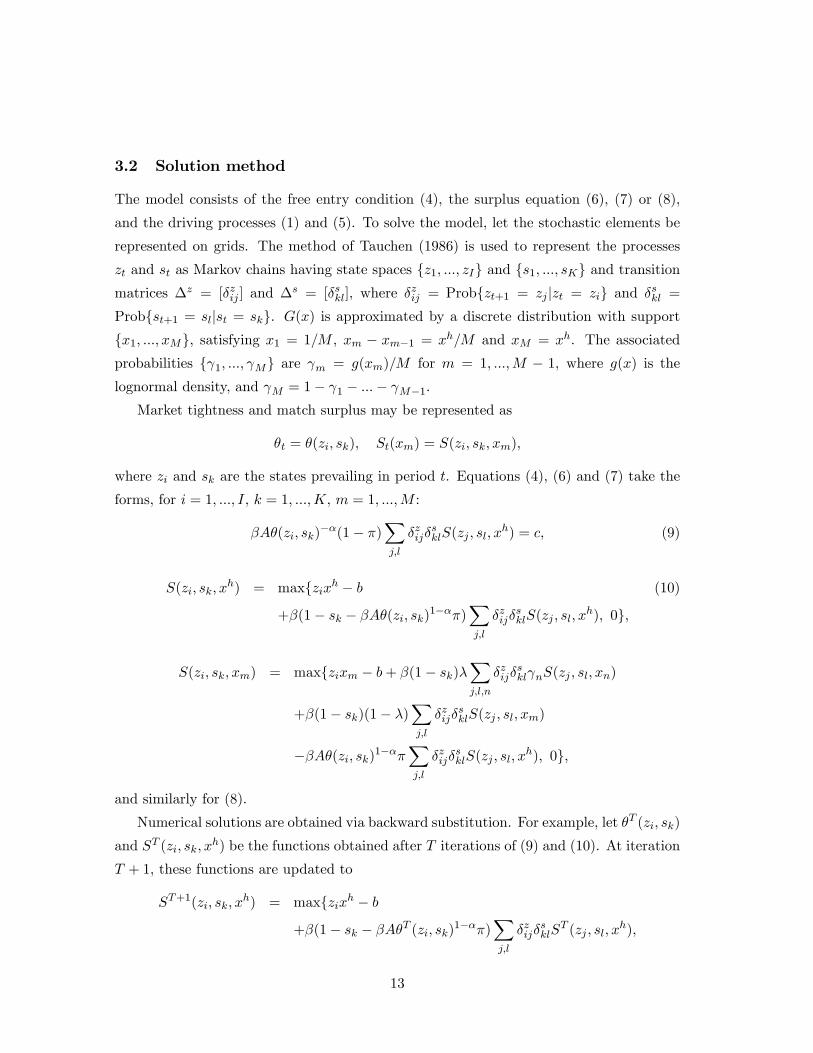
3.2 Solution method

The model consists of the free entry condition (4), the surplus equation (6), (7) or (8),

and the driving processes (1) and (5). To solve the model, let the stochastic elements be

represented on grids. The method of Tauchen (1986) is used to represent the processes

zt and st as Markov chains having state spaces fz1; :::; zIg and fs1; :::; sKg and transitionmatrices �z = [�zij ] and �

s = [�skl], where �zij = Probfzt+1 = zj jzt = zig and �skl =

Probfst+1 = sljst = skg. G(x) is approximated by a discrete distribution with supportfx1; :::; xMg, satisfying x1 = 1=M , xm � xm�1 = xh=M and xM = xh. The associated

probabilities f 1; :::; Mg are m = g(xm)=M for m = 1; :::;M � 1, where g(x) is thelognormal density, and M = 1� 1 � :::� M�1.

Market tightness and match surplus may be represented as

�t = �(zi; sk); St(xm) = S(zi; sk; xm);

where zi and sk are the states prevailing in period t. Equations (4), (6) and (7) take the

forms, for i = 1; :::; I, k = 1; :::;K, m = 1; :::;M :

�A�(zi; sk)��(1� �)

Xj;l

�zij�sklS(zj ; sl; x

h) = c; (9)

S(zi; sk; xh) = maxfzixh � b (10)

+�(1� sk � �A�(zi; sk)1��)Xj;l


h); 0g;

S(zi; sk; xm) = maxfzixm � b+ �(1� sk)�Xj;l;n

�zij�skl nS(zj ; sl; xn)

+�(1� sk)(1� �)Xj;l

�zij�sklS(zj ; sl; xm)

��A�(zi; sk)1��Xj;l


h); 0g;

and similarly for (8).

Numerical solutions are obtained via backward substitution. For example, let �T (zi; sk)

and ST (zi; sk; xh) be the functions obtained after T iterations of (9) and (10). At iteration

T + 1, these functions are updated to

ST+1(zi; sk; xh) = maxfzixh � b

+�(1� sk � �A�T (zi; sk)1��)Xj;l

�zij�sklS

T (zj ; sl; xh);

13

�T+1(zi; sk) =

0@�A(1� �)c

Xj;l

�zij�sklS

T+1(zj ; sl; xh)

1A 1�

:

Convergence follows as a consequence of the saddlepoint stability property of the matching

model, which makes for stability in the backward dynamics.8

3.3 Empirical data

The empirical data series used for purposes of model evaluation are constructed as follows.

Employment, unemployment, job �nding and separation rates, and UE and EU �ows are

quarterly averages of the monthly series from Fujita and Ramey (2006), covering 1976Q2-

2005Q4. The productivity series is obtained by dividing quarterly GDP by the employment

series. Vacancies are measured as quarterly averages of the Conference Board�s monthly

Help Wanted Index. All quarterly series are logged and HP �ltered, with a smoothing

parameter of 1600. Summary statistics used for calibration and model evaluation are

listed in the �rst column of Table 2.

It is well known that the CPS data are subject to potential biases stemming from clas-

si�cation error and sample attrition.9 Importantly, the magnitudes of measured monthly

worker transitions are comparable to the number of observations lost through attrition.

If attrition is subject to cyclical in�uences, then the measured cyclicality of gross �ows

and transition rates may give a misleading picture of true cylicality.

To assess this issue, an alternative data source, the Survey on Income and Program

Participation (SIPP), is considered. Since the SIPP tracks individual respondents across

time, it is subject to minimal sample attrition. Fujita, et al. (2007) have used the SIPP

data to construct gross �ow and transition rate series that conform to the CPS measure-

ment concepts. These "synthetic CPS series" may be compared to the corresponding CPS

series to gauge the robustness of the CPS evidence.10

Columns two and three of Table 2 compare statistics derived from the SIPP-based syn-

thetic CPS series with statistics from the actual CPS series, calculated over the restricted

8 In solving the model, I = K = 13 and M = 200 are chosen. The tolerance for pointwise convergence

of �(zi; sk) and S(zi; sk; xm) is 10�8.9These issues are discussed in Abowd and Zellner (1985), Blanchard and Diamond (1990) and Moscarini

and Thomsson (2007), for example.10Since our 2007 draft, Chris Nekarda has implemented two minor changes in the construction of the

synthetic CPS series, involving the assignment of unemployed status and aggregation across SIPP panels.

The current analysis uses these revised series.

14

SIPP sample period of 1983:Q3-2003:Q4. While the worker �ows and transition rates are

considerably more variable in the SIPP, the relative magnitudes of standard deviations

across the four series JFR, SR, UE flows and EU flows are comparable, although JFR

is somewhat less variable in the SIPP. Importantly, the series SR and EU flows exhibit

nearly identical negative correlations with productivity in both data sets. This suggests

that sample attrition does not serve to bias the measured cyclicality of employment out-

�ows in the CPS. On the other hand, JFR is negatively correlated with productivity in

the SIPP, in contrast to the weak positive correlation observed in the CPS.

This comparison provides compelling evidence that the observed negative correlation

between the separation rate and productivity is not an artifact of measurement problems

in the CPS.

3.4 Evaluation procedure

To conform with the empirical series, the simulated weekly data are averaged to quarterly

frequency, logged and HP �ltered using the same smoothing parameter. Each simulated

quarterly series consists of 619 observations, of which the last 119 are used to calculate

the reported statistics. For each of the four speci�cations, 1000 replications are run, and

averages of the statistics across the replications are presented in the �gures.

4 Results

4.1 Unemployment and worker transition rates

Panel A of Figure 1 compares the empirical standard deviations of unemployment and

worker transition rates with the values obtained from the four speci�cations of the MP

model. The empirical standard deviation of unemployment, equalling 9.5 percent, is over

eight times greater than the value of roughly 1.2 percent generated by the constant sepa-

ration rate speci�cation. This conforms to the observation of Costain and Reiter (2006)

and Shimer (2005) that the MP model with a constant separation rate produces far too

little unemployment volatility.

However, the empirical separation rate is not in fact constant, as it has a standard

deviation of 5.8 percent. The other three versions of the MP model, which allow for

�uctuations in the separation rate, are calibrated to match the latter standard deviation.

All three speci�cations yield signi�cantly greater unemployment volatility. The standard

15

deviation of unemployment in the OJS speci�cation, in particular, is 6.2 percent, or over 60

percent of its empirical value. Thus, incorporating variability at the separation margin,

under any of the three speci�cations, greatly enhances the ability of the MP model to

produce realistic unemployment volatility.

At the same time, all four speci�cations of the MP model yield highly unrealistic

volatility of the job �nding rate, with the empirical standard deviation being nearly six

times the simulated value in each speci�cation. Improving the model�s performance at the

separation margin does not mitigate its problems at the job �nding margin.

Panel B of Figure 1 presents contemporaneous correlations with productivity. The

constant, endogenous and OJS speci�cations each produce strong negative comovement

between unemployment and productivity, in line with the data, while the AR(1) speci-

�cation generates little comovement. All four speci�cations give rise to strong positive

productivity comovement for the job �nding rate. The two exogenous separation speci�-

cations, however, fail to replicate the negative correlation between productivity and the

separation rate that is a robust feature of the data. The two endogenous separation rate

speci�cations succeed in capturing this negative correlation.

Elasticities of the variables with respect to productivity are shown in Panel C.11 The

productivity elasticities o¤er clearer measures of comovement, insofar as they re�ect the

e¤ects of variations in productivity in isolation from other disturbances; see Mortensen and

Nagypál (2007a). The elasticities may also be interpreted as rough measures of respon-

siveness to productivity shocks. For unemployment, the empirical productivity elasticity

of -6.5 is over six times greater in magnitude than the elasticities produced by the two

exogenous separation speci�cations. However, each of the endogenous separation speci�-

cations achieves a close match with the empirical elasticity; the value for the OJS model,

in particular, comes in at -6.2.

Findings are similar for the separation rate elasticities, where the exogenous separation

speci�cations provide highly unrealistic values, while those of the endogenous separation

speci�cations are empirically reasonable. Across all four speci�cations, however, the pro-

ductivity elasticities of the job �nding rate are far too low: the empirical value is 4.0, while

the simulated values do not exceed 1.4.

In summary, introducing variability at the separation margin greatly magni�es the

degree of unemployment volatility generated by the MP model, whether the separation

11These productivity elasticities are computed as follows. Let pt denote productivity in quarter t, and

let yt be any series. Then the productivity elasticity is Corr(pt; yt)SD(yt)=SD(pt).

16

rate is determined exogenously or endogenously. Moreover, when the separation rate

is endogenous, the model generates realistic responsiveness of unemployment and the

separation rate to productivity shocks, whereas the exogenous separation versions yield

little or no responsiveness. For all of the speci�cations considered, the simulated job

�nding rate is de�cient in both its volatility and its responsiveness to productivity.

4.2 Worker �ows

Figure 2 considers gross �ows of workers between unemployment and employment. As

Panel A indicates, the constant separation rate speci�cation produces almost no volatility

in UE and EU �ows. This is contrary to the data, where the standard deviations for

both �ows are roughly half of the value for unemployment. The three speci�cations with

variable separation rates, in contrast, do a good job in matching the empirical standard

deviations of both UE and EU �ows. Thus, variability at the separation margin appears

to be crucial for producing realistic variability in worker �ows.

Panel B shows that with constant separation rates, worker �ows exhibit a strong

positive correlation with productivity. This contradicts the substantial negative correlation

seen in the data. In the constant separation rate model, worker �ows are driven principally

by procyclical movements in the job �nding rate, allowing little scope for explaining their

observed countercyclical movements. The AR(1) model, in turn, yields essentially acyclical

movements in worker �ows, re�ecting the fact that exogenous separation rate shocks are

uncorrelated with the productivity process.

The two endogenous separation rate speci�cations, on the other hand, produce strong

negative correlations between productivity and worker �ows. Overall, as Panel C re-

veals, worker �ows are almost entirely unresponsive to productivity in the two exogenous

separation rate speci�cations, whereas they exhibit strong negative responses in the two

endogenous separation speci�cations.

4.3 Vacancies and market tightness

Vacancies and market tightness are considered in Figure 3. Panel A shows that all four

speci�cations imply insu¢ cient volatility of both vacancies and market tightness, consis-

tent with the low volatility of the job �nding rate observed in Figure 1. The standard

deviation of market tightness in the OJS model is signi�cantly greater than in the other

speci�cations, however. This occurs because empirical market tightness is measured as va-

17

cancies divided by unemployment, whereas the variable �t also includes employed searching

workers in its denominator. Thus, the empirical measure omits procyclical movements in

the number of employed searchers that o¤set countercyclical movements in unemployment,

leading to greater variability of the measured ratio.

Panel B depicts the productivity correlations. Both versions of the exogenous separa-

tion model replicate the procyclical movements of vacancies seen in the data, whereas the

endogenous separation model without OJS yields countercyclical movements. The latter

�nding re�ects con�icting e¤ects on the incentive to post vacancies. Following a nega-

tive productivity shock, the returns to forming a new match are relatively low, reducing

vacancy posting incentives. This e¤ect drives vacancies downward in the constant and

AR(1) models. In the endogenous separation model without OJS, however, the separation

rate rises in response to the productivity shock, pushing up the number of unemployed

workers. This increases the vacancy matching probability and enhances the incentive to

post vacancies. On balance, the latter e¤ect dominates, and vacancies become negatively

correlated with productivity.

The OJS model, however, produces a strong positive correlation between vacancies and

productivity, despite the fact that the separation rate is determined endogenously. With

OJS, a negative productivity shock induces a fall in the number of employed searchers

which partially o¤sets the rise in unemployment. Thus, endogenous separation is consis-

tent with realistic vacancy comovement once OJS is incorporated. Note �nally that all

four speci�cations yield positive productivity comovement for market tightness, in line

with the data.

Productivity elasticities are shown in Panel C. The empirical productivity elasticity

of vacancies far exceeds the elasticities obtained from the three speci�cations without

OJS. In the OJS speci�cation, however, the elasticity of vacancies amounts to over half

of its empirical value. Thus, incorporating OJS greatly improves the ability of the model

to match the productivity responsiveness of vacancies. For market tightness, the OJS

model performs even better, as the simulated productivity elasticity amounts to nearly

75 percent of the empirical value. Thus, while variability and productivity responsiveness

are insu¢ cient for all four speci�cations of the MP model, the OJS version signi�cantly

improves on the others. The superior performance of the OJS speci�cation results from

procyclical variations in the number of searching workers, which make vacancies more

responsive to productivity at given levels of market tightness.

18

4.4 Beveridge correlation

Panel A of Figure 4 presents contemporaneous correlations between unemployment and

vacancies, capturing the Beveridge curve relationship. The value of -0.95 observed in the

data is reasonably well matched by the value -0.76 generated by the constant separation

rate speci�cation. The AR(1) speci�cation, in contrast, produces a highly counterfactual

value of 0.75, and for the endogenous separation speci�cation the value is an even more

unrealistic 0.92. In the AR(1) model, a small positive separation rate shock induces a

large in�ow into unemployment, because the stock of employed workers is relatively large.

Workers become easier to �nd, while productivity is unchanged, so incentives to post

vacancies rise. A related e¤ect operates in the endogenous separation model, where a

negative productivity shock drives up unemployment, making workers easier to �nd and

raising the incentive to post vacancies.

For the OJS model, the unemployment-vacancy correlation amounts to -0.96, nearly

indistinguishable from the empirical value. Here, procyclical movements in the number of

employed searchers lead to procyclical changes in vacancy posting incentives, giving rise

to a realistic Beveridge correlation.

4.5 Transition rate comovement

Contemporaneous correlations between job �nding and separation rates are depicted in

panel B of Figure 4. In the data, these rates have a negative correlation of about -0.5,

whereas the correlations are essentially zero in the two exogenous separation speci�cations.

The two endogenous separation speci�cations, on the other hand, produce strong negative

correlations, on the order of -0.88. The latter speci�cations achieve the correct transition

rate comovement chie�y because the two rates themselves respond realistically to the

common underlying productivity process.

5 Dynamic interrelationships

5.1 Cross productivity elasticities

Figures 5 through 7 present elasticities with productivity at various leads and lags. To

clarify the discussion, only the constant and OJS speci�cations are considered; �ndings

are qualitatively similar for the other speci�cations.

19

Panel A of Figure 5 shows the elasticities of unemployment with respect to produc-

tivity at each of the given lags; e.g., the reported elasticity at a lag of 1 represents the

correlation between current unemployment and productivity lagged by one quarter, multi-

plied and divided by the appropriate standard deviations. Empirically, the responsiveness

of unemployment to productivity achieves its peak of -8 at a lag of two quarters. For the

OJS model, the peak of just under -6 is reached at a zero to one quarter lag. Thus, the

model fails to produce realistic response dynamics, in that responses occur more quickly

than in the data. A similar �nding can be observed for the constant separation rate model.

Cross productivity elasticities for the job �nding rate are given in panel B. The empiri-

cal job �nding rate responds more slowly than does unemployment, with the peak elasticity

occurring at a lag of three quarters. For both speci�cations of the MP model, in contrast,

the elasticities peak sharply at zero lag. Thus, while the actual productivity responses of

the job �nding rate are spread out across time, they occur more or less contemporaneously

with productivity in the MP model. Cross elasticities for vacancies and market tightness,

shown in Figure 7, display similar properties. As stressed by Fujita and Ramey (2007), the

fact that vacancies can jump instantaneously in the MP model causes market tightness

to respond too quickly to productivity shocks. This undermines the model�s ability to

generate realistic dynamic responses of unemployment, the job �nding rate, vacancies and

market tightness.

Panel C of Figure 5 depicts the cross elasticities for the separation rate, while the cross

elasticities for UE and EU �ows are given in Figure 6. In these instances, the OJS model

does a reasonable job of matching the empirical response pattern: the separation rate and

EU �ows adjust contemporaneously with productivity or lead it slightly, while UE �ows

lag productivity by about a quarter. In the constant separation rate model, in contrast,

these variables are essentially unresponsive to productivity at all leads and lags.

In summary, the MP model with endogenous separation yields sensible dynamics of

the separation rate and worker �ows, whereas the responses of unemployment, the job

�nding rate, vacancies and market tightness are insu¢ ciently sluggish. In no case does

the model with exogenous separation deliver a realistic pattern of responses.

5.2 Beveridge correlations

Cross correlations between unemployment and vacancies are given in panel A of Figure

8. While both the constant and OJS speci�cations provide strong negative Beveridge

20

correlations, in the constant separation rate model the peak correlation is achieved at a

lead of one quarter, i.e., vacancies lead unemployment by one quarter, whereas in the data

the peak occurs at zero lag. This re�ects the mechanics of the model, wherein changes in

unemployment are driven by changes in the job �nding rate, which themselves are tied to

�uctuations in vacancies. The OJS model, on the other hand, exhibits its peak correlation

at zero lag, and matches fairly well the dynamic pattern seen in the data.

5.3 Transition rate correlations

Panel B of Figure 8 reports the cross correlations of job �nding and separation rates. In

the data, strong negative correlations are achieved at lags of -1 to �4 quarters, meaning

that the separation rate leads the job �nding rate. While the correlations for the OJS

model exhibit a slight negative phase shift, they fail to capture adequately the overall

dynamic pattern. Of course, all of these correlations are zero in the constant separation

rate model.

6 Hagedorn-Manovskii calibration

Hagedorn and Manovskii (2008, henceforth HM) propose an alternative approach to cal-

ibrating the MP model that draws on wage and pro�t data. In all four speci�cations of

the MP model, the wage rate determined by Nash bargaining is

wt(x) = (1� �)b+ �(ztx+ �tc);

where x is identically equal to xh in the exogenous separation speci�cations. HM point out

that under standard calibrations, the empirical productivity elasticity of wages is much

lower than the elasticity generated by the model. They propose an alternative calibration

strategy that aims to match this elasticity, along with the empirical relationship between

mean wage and pro�t levels.

To assess the implications of the HM calibration, this paper follows Hornstein, et

al. (2005) in varying the calibrated values of b and � in order to set the productivity

elasticity of wages and the steady state wage-productivity ratio to the values 0.5 and 0.97,

respectively. For brevity, only the constant and OJS speci�cations are considered.

The new calibrations are reported in columns �ve and six of Table 1. As noted by

Hornstein, et al., matching the empirical statistics requires large increases in the b para-

meter and large decreases in the � parameter. For the constant separation rate model,

21

the A parameter is adjusted to match the mean job �nding rate, while for the OJS model

the parameters xh, s and �x are also adjusted to normalize mean productivity and match

the mean and standard deviation of the separation rate. Importantly, under the HM cal-

ibration the rate of job-to-job transitions is negligible, although still positive, even when

the search cost parameter a is set to zero; the latter value is adopted here. The model is

solved and simulated according to the procedures discussed earlier.

Results are presented in Figures 9 through 12, which parallel Figures 1 through 4 in

their content. Statistics pertaining to the standard calibrations of the constant and OJS

speci�cations, taken from the earlier �gures, are depicted alongside statistics obtained

from the corresponding HM calibrations. Panel A of Figure 9 demonstrates that the HM

calibration produces much more realistic volatility of unemployment and the job �nding

rate for both speci�cations. Moreover, the job �nding rate becomes highly responsive to

productivity, as seen in panel C. The responsiveness of the separation rate in the OJS

model declines considerably, however. This re�ects the fact that, following a negative

productivity shock, strong downward movement in the job �nding rate reduces separation

incentives by degrading workers�outside option.

Figure 10 reveals that the HM calibration enhances the volatility of UE �ows in the

constant separation rate model, but it does not appreciably raise the volatility of EU

�ows, nor does it mitigate the counterfactual procyclicality of worker �ows implied by this

speci�cation. Moreover, worker �ows become less responsive to productivity in the OJS

model. For UE �ows, in particular, strong procyclical movements in the job �nding rate

serve to neutralize the countercyclical movements in the separation rate, leaving virtually

no responsiveness to productivity.

The HM calibration greatly improves the performance of both speci�cations in match-

ing the empirical features of vacancies and market tightness, as Figure 11 demonstrates.

Finally, the Beveridge and transition rate correlations are presented in Figure 12. These

are essentially una¤ected for the constant separation rate model, while they become some-

what smaller in magnitude for the OJS model. Under the HM calibration, matching the

empirical standard deviation of the separation rate necessitates a smaller role for �uc-

tuations at the OJS margin, so that procyclical adjustments in the number of employed

searchers do not work as strongly to o¤set countercyclical unemployment movements. The

Beveridge correlation nonetheless remains substantially negative.

22

7 Conclusion

This paper considers four speci�cations of the standard MP model that di¤er in how they

treat the separation margin. The speci�cations are calibrated at weekly frequency and

solved using a nonlinear method. Allowing for realistic time variation of the separation rate

greatly increases the volatility of unemployment in the simulated data. In the speci�cation

with OJS, for example, the standard deviation of unemployment equals 60 percent of its

empirical value. Thus, moving beyond constant separation rates goes a long way towards

redressing the problem of insu¢ cient unemployment volatility in the MP model.

Both of the speci�cations with exogenous separation rates fail to reproduce the em-

pirical volatility and productivity responsiveness of the separation rate and worker �ows.

The endogenous separation speci�cations, in contrast, yield empirically reasonable be-

havior along these dimensions, and the speci�cation with OJS also generates a realistic

Beveridge curve correlation. Furthermore, the endogenous separation speci�cations imply

more realistic dynamic interrelationships in comparison to the exogenous separation ones.

Two broad conclusions emerge from this analysis. First, the endogenous separation

speci�cation with OJS dominates both of the exogenous separation speci�cations along all

dimensions considered. From the empirical standpoint, there seems to be no justi�cation

for assuming exogenous separation when modelling the separation margin.

Second, the OJS version of the MP model, as articulated in Pissarides (2000), does

a remarkable job in matching labor market facts even under the standard calibration,

although the model still generates insu¢ cient volatility of the job �nding rate and related

variables. Adopting the HM calibration largely resolves the latter failings, but it fails to

generate a realistic volume of job-to-job transitions.

The inability of the MP model to generate sluggish dynamics suggests that it does

not deal adequately with key structural features of the labor market. Fujita and Ramey

(2007) argue that �xed costs of vacancy creation may be salient in practice, and they

show that introducing these costs into the MP model with constant separation rates leads

to substantial improvements in its dynamic performance. Further investigations in this

direction might lead to a more complete resolution of this issue.

23

References

Abowd, John M. and Zellner, Arnold. "Estimating Gross Labor Force Flows." Journal of

Business and Economic Statistics, June 1985, 3(3), pp. 254-83.

Andolfatto, David. �Business Cycles and labor-Market Search.�American Economic Re-

view, March 1996, 86(1), pp. 112-32.

Barron, John M., Berger, Mark C., and Black, Dan A. �Employer Search, Training, and

Vacancy Duration.�Economic Inquiry, January 1997, 35(1), 167-92.

Barron, John M., and Bishop, John. �Extensive Search, Intensive Search, and Hiring

Costs: New Evidence on Employer Hiring Activity.�Economic Inquiry, July 1985, 23(3),

363-82.

Blanchard, Olivier Jean, and Diamond, Peter. "The Cyclical Behavior of the Gross Flows

of U.S. Workers." Brookings Papers on Economic Activity, 1990(2), pp. 85-143.

Cooley, Thomas F., and Quadrini, Vincenzo. �A Neoclassical Model of the Phillips Curve

Relationship.�Journal of Monetary Economics, October 1999, 44(2), 165-93.

Costain, James S., and Reiter, Michael. �Business Cycles, Unemployment Insurance, and

the Calibration of Matching Models.�Draft, Bank of Spain and Universitat Pompeu Fabra,

October 2006.

Cole, Harold L., and Rogerson, Richard. �Can the Mortensen-Pissarides Matching Model

Match the Business Cycle Facts?�International Economic Review, November 1999, 40(4),

933-59.

Den Haan, Wouter J., Ramey, Garey, and Watson, Joel. �Job Destruction and Propaga-

tion of Shocks.�American Economic Review, June 2000, 90(3), pp. 482-98.

Farmer, Roger E.A., and Hollenhorst, Andrew. �Shooting the Auctioneer.�Draft, UCLA,

August 2006.

Fujita, Shigeru. �The Beveridge Curve, Job Creation, and the Propagation of Shocks.�

Draft, UCSD, 2003.

24

Fujita, Shigeru. �Vacancy Persistence.�Working Paper No, 04-23, Federal Reserve Bank

of Philadelphia, October 20, 2004.

Fujita, Shigeru and Ramey, Garey. �The Cyclicality of Job Loss and Hiring.� Federal

Reserve Bank of Philadelphia Working Paper 06-17, November 2006.

Fujita, Shigeru and Ramey, Garey. �Job Matching and Propagation.�Journal of Economic

Dynamics and Control, November 2007, 31(11), pp. 3671-98.

Fujita, Shigeru; Nekarda, Christopher J. and Ramey, Garey. "The Cyclicality of Worker

Flows: New Evidence from the SIPP" Federal Reserve Bank of Philadelphia Working

Paper 07-05, February 2007.

Gertler, Mark, and Trigari, Antonella. �Unemployment Fluctuations with Staggered Nash

Wage Bargaining.�Draft, NYU and Università Bocconi, July 2006.

Hagedorn, Marcus, and Manovskii, Iourii. �The Cyclical Behavior of Equilibrium Unem-

ployment and Vacancies Revisited.�American Economic Review, forthcoming.

Hall, Robert E. �Employment Fluctuations with Equilibrium Wage Stickiness.�American

Economic Review, March 2005, 95(1), pp. 50-65.

Hall, Robert E. �The Labor Market and Macro Volatility: A Nonstationary General Equi-

librium Analysis.�Draft, Stanford University, April 9, 2006.

Hornstein, Andreas, Krusell, Per, and Violante, Giovanni L. �Unemployment and Vacancy

Fluctuations in the Matching Model: Inspecting the Mechanism.�Federal Reserve Bank

of Richmond Economic Quarterly, Summer 2005, 91(3), pp. 19-51.

Krause, Michael U. and Lubik, Thomas A. �The Cyclical Upgrading of Labor and On-

the-Job Search.�Labour Economics, August 2006, 13(4), pp. 459-77.

Krause, Michael U. and Lubik, Thomas A. �The (Ir)relevance of Real Wage Rigidity in

the New Keynesian Model with Search Frictions.�Journal of Monetary Economics, April

2007, 54(3), pp. 706-27.

Menzio, Guido and Shi, Shouyong. "E¢ cient Search on the Job and the Business Cycle."

Draft, University of Pennsylvania and University of Toronto, August 2008.

25

Merz, Monika. �Search in the Labor Market and the Real Business Cycle.� Journal of

Monetary Economics, November 1995, 36(2), pp. 269-300.

Mortensen, Dale T. �The Cyclical Behavior of Job and Worker Flows.� Journal of Eco-

nomic Dynamics and Control, November 1994, 18(6), pp. 1121-42.

Mortensen, Dale T. �More on Unemployment and Vacancy Fluctuations.�Discussion Pa-

per No. 1765, IZA, September 2005.

Mortensen, Dale T., and Nagypál, Éva. �More on Unemployment and Vacancy Fluctua-

tions.�Review of Economic Dynamics, July 2007a, 10(3), pp. 327-47.

Mortensen, Dale T. and Nagypál, Éva. "Labor-market Volatility in Matching Models with

Endogenous Separations." Scandinavian Journal of Economics, December 2007b, 109(4),

pp. 645-65.

Mortensen, Dale T. and Pissarides, Christopher A. �Job Creation and Job Destruction

in the Theory of Unemployment.� Review of Economic Studies, July 1994, 61(3), pp.

397-415.

Moscarini, Giuseppe and Thomsson, Kaj. "Occupational and Job Mobility in the U.S."

Scandinavian Journal of Economics, December 2007, 109(4), pp. 807-36.

Nagypál, Éva. "On the Extent of Job-to-Job Transitions." Draft, Northwestern University,

September 2005a.

Nagypál, Éva. "Labor-Market Fluctuations, On-the-Job Search, and the Acceptance

Curse." Draft, Northwestern University, December 6, 2005b.

Pissarides, Christopher A. �Search Unemployment with On-the-Job Search.�Review of

Economic Studies, July 1994, 61(3), pp. 457-75.

Pissarides, Christopher A. Equilibrium Unemployment Theory. Cambridge, MA: MIT

Press, 2000.

Pissarides, Christopher A.. �The Unemployment Volatility Puzzle: Is Wage Stickiness the

Answer?�Draft, LSE, June 22, 2007.

26

Rotemberg, Julio. �Cyclical Wages in a Search-and-Bargaining Model with Large Firms.�

Draft, Harvard Business School, February 27, 2006.

Shimer, Robert. �The Cyclical Behavior of Equilibrium Unemployment and Vacancies.�

American Economic Review, March 2005, 95(1), pp. 25-49.

Tasci, Murat. �On-the-Job Search and Labor Market Reallocation.�Draft, University of

Texas at Austin, February 13, 2006.

Tauchen, George. �Finite State Markov-Chain Approximations to Univariate and Vector

Autoregressions.�Economics Letters, 1986, 20(2), pp. 177-81.

Walsh, Carl E. �Labor Market Search and Monetary Shocks.�In Altug, Sumru, Chandha,

Jagjit S., and Nolan, Charles, eds. Dynamic Macroeconomic Analysis: Theory and Policy

in General Equilibrium. Cambridge: Cambridge University Press, 2003.

Walsh, Carl E. �Labor Market Search, Sticky Wages, and Interest Rate Policies.�Review

of Economic Dynamics, October 2005, 8(4), pp. 829-849.

Yashiv, Eran. �Evaluating the Performance of the Search and Matching Model.�European

Economic Review, May 2006a, 50(4), pp. 909-36.

27

Table 1 Parameter values Parameter Const AR(1) Endog OJS Const–HM OJS-HM

b 0.7 0.7 0.7 0.7 0.955 0.934 c 0.17 0.17 0.17 0.17 0.17 0.17 a - - - 0.174 - 0 A 0.083 0.083 0.081 0.081 0.068 0.056 α 0.6 0.6 0.6 0.6 0.6 0.6 π 0.6 0.6 0.6 0.6 0.07 0.062 hx 1.00 1.00 1.17 1.18 1.00 1.13 s 0.005 0.005 0.0015 0.004 0.005 0.0048 sρ 0 0.97 - - - - sσ 0 0.0168 - - - - λ - - 0.085 0.085 - 0.085 xµ - - 0 0 - 0 xσ - - 0.2275 0.2270 - 0.1426 zρ 0.99 0.99 0.99 0.99 0.99 0.99 zσ 0.0027 0.0027 0.0027 0.0027 0.0027 0.0027 β 0.9992 0.9992 0.9992 0.9992 0.9992 0.9992 Parameters: b : unemployment payoff. c : vacancy posting cost. a : OTJ search cost. α,A : parameters of matching function. π : worker bargaining weight. hx : highest value of match-specific productivity factor. s : mean exogenous separation probability. ss σρ , : parameters of exogenous separation process. xx σµλ ,, : parameters of match-specific productivity process. zz σρ , : parameters of aggregate productivity process. β : discount factor. See text for explanation of calibration procedure. Specifications: Const: constant separation rate model. AR(1): AR(1) separation rate model. Endog: endogenous separation rate model without OJS. OJS: endogenous separation rate model with OJS. Const-HM: constant separation rate model, Hagedorn-Manovskii calibration. OJS-HM: endogenous separation rate model with OJS, Hagedorn-Manovskii calibration.

Table 2 Empirical statistics CPS SIPP CPS (1976Q2-2005Q4) (1983Q3-2003Q4) (1983Q3-2003Q4) Standard deviations Unempl. .0959 .0980 .0766 JFR .0784 .1068 .0655 SR .0577 .1174 .0439 UE flows .0421 .1025 .0388 EU flows .0530 .1143 .0413 Mkt. tightness .2164 .1762 .1636 Productivity correlations Unempl. -.4850 -.1796 -.2504 JFR .3626 -.2833 .1589 SR -.5791 -.3407 -.3119 UE flows -.3738 -.5067 -.1616 EU flows -.5661 -.3431 -.3101 Mkt. tightness .5569 .3536 .3437 Other correlations Vac.-Unempl. -.9532 -.6779 -.9017 JFR-SR -.5082 -.0584 -.3027 Variables: Unempl: unemployment rate. JFR: job finding rate. SR: separation rate. UE flows: gross flows from U to E. EU flows: gross flows from E to U. Mkt. tightness: ratio of vacancies to unemployment. Vac.: job vacancies. See text for variable definitions. Notes: CPS data are from Fujita and Ramey (2006). SIPP data are from Fujita, Nekarda and Ramey (2007). Vacancies are measured by the Conference Board’s Help-Wanted Advertising Index. Productivity is measured as chain-weighted real GDP divided by employment. Hazard rate and gross flow series are adjusted for margin error and time aggregation error. All series are quarterly, logged and HP filtered, with smoothing parameter 1600.

Figure 1. Unemployment and worker transition rates

A. Standard deviations

0

0.02

0.04

0.06

0.08

0.1

0.12

Unemployment JFR SR

DataConstAR(1)EndogOJS

B. Productivity correlations

-1

-0.5

0

0.5

1

Unemployment JFR SR


C. Productivity elasticities

-7

-5

-3

-1

1

3

5

Unemployment JFR SR


Notes: Data: quarterly averages of monthly CPS series, 1976Q2-2005Q4, from Fujita and Ramey (2006). Series are logged and HP filtered, with smoothing parameter 1600. Statistics are taken from Table 2. Const: constant separation rate model. AR(1): AR(1) separation rate model. Endog: endogenous separation rate model without OJS. OJS: endogenous separation rate model with OJS. See Table 1 for calibrations. Simulated data are quarterly averages of weekly series, logged and HP filtered, with smoothing parameter 1600. Each replication computes simulated statistics from a sample of 119 quarterly observations. Reported statistics are averages over 1000 replications.

Figure 2. Worker flows


0

0.01

0.02

0.03

0.04

0.05

0.06

UE flows EU flows



-1

-0.5

0

0.5

1

UE flows EU flows



-6

-5

-4

-3

-2

-1

0

1

UE flows EU flows DataConstAR(1)EndogOJS


Figure 3. Vacancies and market tightness


0

0.05

0.1

0.15

0.2

0.25

Vacancies Market tightness



-1

-0.5

0

0.5

1




-5

0

5

10

15

20




Figure 4. Contemporaneous correlations

A. Unemployment and vacancies

-1

-0.5

0

0.5

1


B. Job finding and separation rates

-1

-0.5

0

0.5

1



Figure 5. Cross elasticities with productivity: Unemployment and worker transition rates

A. Unemployment

-10

-8

-6

-4

-2

0

2

-4 -3 -2 -1 0 1 2 3 4

DataConstOJS

B. Job finding rate

-3-2-101234567

-4 -3 -2 -1 0 1 2 3 4

DataConstOJS

C. Separation rate

-7

-6

-5

-4

-3

-2

-1

0-4 -3 -2 -1 0 1 2 3 4

DataConstOJS

Notes: Graphs show correlations between variables at t and productivity at t-i, where i = abscissa. Data: quarterly averages of monthly CPS series, 1976Q2-2005Q4, from Fujita and Ramey (2006). Series are logged and HP filtered, with smoothing parameter 1600. Statistics are taken from Table 2. Const: constant separation rate model. OJS: endogenous separation rate model with OJS. See Table 1 for calibrations. Simulated data are quarterly averages of weekly series, logged and HP filtered, with smoothing parameter 1600. Each replication computes simulated statistics from a sample of 119 quarterly observations. Reported statistics are averages over 1000 replications.

Figure 6. Cross elasticities with productivity: Worker flows

A. UE flows

-6

-5

-4

-3

-2

-1

0

1

-4 -3 -2 -1 0 1 2 3 4

DataConstOJS

B. EU flows

-7

-6

-5

-4

-3

-2

-1

0

1

-4 -3 -2 -1 0 1 2 3 4

DataConstOJS


Figure 7. Cross elasticities with productivity: Vacancies and market tightness

A. Vacancies

-2

0

2

4

6

8

10

12

-4 -3 -2 -1 0 1 2 3 4

DataConstOJS

B. Market tightness

-5

0

5

10

15

20

-4 -3 -2 -1 0 1 2 3 4

DataConstOJS


Figure 8. Cross correlations


-1

-0.5

0

0.5

1

-4 -3 -2 -1 0 1 2 3 4

DataConstOJS


-1

-0.5

0

0.5

1

-4 -3 -2 -1 0 1 2 3 4

DataConstOJS

Notes: Panel A: correlations between vacancies at t and unemployment at t-i, where i = abscissa. Panel B: correlations between separation rate at t and job finding rate rate at t-i. Data: quarterly averages of monthly CPS series, 1976Q2-2005Q4, from Fujita and Ramey (2006). Series are logged and HP filtered, with smoothing parameter 1600. Statistics are taken from Table 2. Const: constant separation rate model. AR(1): AR(1) separation rate model. Endog: endogenous separation rate model without OJS. OJS: endogenous separation rate model with OJS. See Table 1 for calibration. Simulated data are quarterly averages of weekly series, logged and HP filtered, with smoothing parameter 1600. Each replication computes simulated statistics from a sample of 119 quarterly observations. Reported statistics are averages over 1000 replications.

Figure 9. Unemployment and worker transition rates: Standard and HM calibrations


0

0.02

0.04

0.06

0.08

0.1

0.12

Unemployment JFR SR

DataConstConst - HMOJSOJS - HM


-1

-0.5

0

0.5

1

Unemployment JFR SR



-8-6-4-202468

10

Unemployment JFR SR


Notes: Data: quarterly averages of monthly CPS series, 1976Q2-2005Q4, from Fujita and Ramey (2006). Series are logged and HP filtered, with smoothing parameter 1600. Statistics are taken from Table 2. Const: constant separation rate model. Const-HM: constant separation rate model, HM calibration. OJS: endogenous separation rate model with OJS. OJS-HM: endogenous separation rate model with OJS, HM calibration. See Table 1 for calibrations. Simulated data are quarterly averages of weekly series, logged and HP filtered, with smoothing parameter 1600. Each replication computes simulated statistics from a sample of 119 quarterly observations. Reported statistics are averages over 1000 replications.

Figure 10. Worker flows: Standard and HM calibrations


0

0.01

0.02

0.03

0.04

0.05

0.06

UE flows EU flows



-1

-0.5

0

0.5

1

UE flows EU flows



-8

-6

-4

-2

0

2

4

UE flows EU flows



Figure 11. Vacancies and market tightness: Standard and HM calibrations


0

0.05

0.1

0.15

0.2

0.25

0.3




-1

-0.5

0

0.5

1




0

5

10

15

20

25




Figure 12. Contemporaneous correlations: Standard and HM calibrations


-1

-0.5

0

0.5

1



-1

-0.5

0

0.5

1



exogenous vs. endogenous separation · exogenous vs. endogenous separation garey ramey december...

Documents