expectation maximization - university of washington

1

1

Expectation Maximization

Machine Learning – CSE546 Carlos Guestrin University of Washington

November 13, 2014 ©Carlos Guestrin 2005-2014

E.M.: The General Case n  E.M. widely used beyond mixtures of Gaussians

¨  The recipe is the same…

n  Expectation Step: Fill in missing data, given current values of parameters, θ(t) ¨  If variable y is missing (could be many variables) ¨  Compute, for each data point xj, for each value i of z:

n  P(z=i|xj,θ(t))

n  Maximization step: Find maximum likelihood parameters for (weighted) “completed data”: ¨  For each data point xj, create k weighted data points

n 

¨  Set θ(t+1) as the maximum likelihood parameter estimate for this weighted data

n  Repeat ©Carlos Guestrin 2005-2014 2

2

3

The general learning problem with missing data

n  Marginal likelihood – x is observed, z is missing:

©Carlos Guestrin 2005-2014

4

E-step

n  x is observed, z is missing n  Compute probability of missing data given current choice of θ

¨  Q(z|xj) for each xj n  e.g., probability computed during classification step n  corresponds to “classification step” in K-means


3

5

Jensen’s inequality

n  Theorem: log ∑z P(z) f(z) ≥ ∑z P(z) log f(z)


6

Applying Jensen’s inequality

n  Use: log ∑z P(z) f(z) ≥ ∑z P(z) log f(z)


4

7

The M-step maximizes lower bound on weighted data

n  Lower bound from Jensen’s:

n  Corresponds to weighted dataset: ¨  <x1,z=1> with weight Q(t+1)(z=1|x1) ¨  <x1,z=2> with weight Q(t+1)(z=2|x1) ¨  <x1,z=3> with weight Q(t+1)(z=3|x1) ¨  <x2,z=1> with weight Q(t+1)(z=1|x2) ¨  <x2,z=2> with weight Q(t+1)(z=2|x2) ¨  <x2,z=3> with weight Q(t+1)(z=3|x2) ¨  …


8

The M-step

n  Maximization step:

n  Use expected counts instead of counts: ¨  If learning requires Count(x,z) ¨ Use EQ(t+1)[Count(x,z)]


5

9

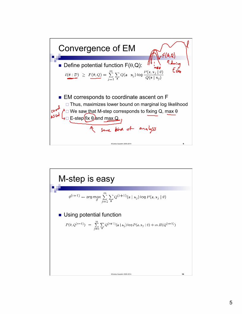
Convergence of EM

n  Define potential function F(θ,Q):

n  EM corresponds to coordinate ascent on F ¨ Thus, maximizes lower bound on marginal log likelihood ¨ We saw that M-step corresponds to fixing Q, max θ ¨ E-step fix θ and max Q


10

M-step is easy

n  Using potential function


6

11

E-step also doesn’t decrease potential function 1 n  Fixing θ to θ(t):


12

KL-divergence

n  Measures distance between distributions

n  KL=zero if and only if Q=P ©Carlos Guestrin 2005-2014

7

13

E-step also doesn’t decrease potential function 2

n  Fixing θ to θ(t):


14

E-step also doesn’t decrease potential function 3

n  Fixing θ to θ(t)

n  Maximizing F(θ(t),Q) over Q → set Q to posterior probability:

n  Note that


8

15

EM is coordinate ascent

n  M-step: Fix Q, maximize F over θ (a lower bound on ):

n  E-step: Fix θ, maximize F over Q:

¨  “Realigns” F with likelihood:


16

What you should know

n  K-means for clustering: ¨  algorithm ¨  converges because it’s coordinate ascent

n  EM for mixture of Gaussians: ¨  How to “learn” maximum likelihood parameters (locally max. like.) in

the case of unlabeled data

n  Be happy with this kind of probabilistic analysis n  Remember, E.M. can get stuck in local minima, and

empirically it DOES n  EM is coordinate ascent n  General case for EM


9

17

Dimensionality Reduction PCA

Machine Learning – CSE4546 Carlos Guestrin University of Washington

November 13, 2014 ©Carlos Guestrin 2005-2014

18

Dimensionality reduction

n  Input data may have thousands or millions of dimensions! ¨ e.g., text data has

n  Dimensionality reduction: represent data with fewer dimensions ¨ easier learning – fewer parameters ¨ visualization – hard to visualize more than 3D or 4D ¨ discover “intrinsic dimensionality” of data

n  high dimensional data that is truly lower dimensional


10

19

Lower dimensional projections

n  Rather than picking a subset of the features, we can new features that are combinations of existing features

n  Let’s see this in the unsupervised setting ¨  just X, but no Y


20

Linear projection and reconstruction

x1

x2

project into 1-dimension z1

reconstruction: only know z1,

what was (x1,x2)


11

21

Principal component analysis – basic idea n  Project n-dimensional data into k-dimensional

space while preserving information: ¨ e.g., project space of 10000 words into 3-dimensions ¨ e.g., project 3-d into 2-d

n  Choose projection with minimum reconstruction error


22

Linear projections, a review

n  Project a point into a (lower dimensional) space: ¨ point: x = (x1,…,xd) ¨ select a basis – set of basis vectors – (u1,…,uk)

n  we consider orthonormal basis: ¨  ui•ui=1, and ui•uj=0 for i≠j

¨ select a center – x, defines offset of space ¨ best coordinates in lower dimensional space defined

by dot-products: (z1,…,zk), zi = (x-x)•ui n  minimum squared error


12

23

PCA finds projection that minimizes reconstruction error n  Given N data points: xi = (x1

i,…,xdi), i=1…N

n  Will represent each point as a projection:

¨  where: and

n  PCA: ¨  Given k<<d, find (u1,…,uk) minimizing reconstruction error:

x1

x2

N

N

N


24

Understanding the reconstruction error

¨ Given k<<d, find (u1,…,uk) minimizing reconstruction error:

N d

n  Note that xi can be represented exactly by d-dimensional projection:

n  Rewriting error:


13

25

Reconstruction error and covariance matrix

N

N

N d


26

Minimizing reconstruction error and eigen vectors

N d

n  Minimizing reconstruction error equivalent to picking orthonormal basis (u1,…,ud) minimizing:

n  Eigen vector:

n  Minimizing reconstruction error equivalent to picking (uk+1,…,ud) to be eigen vectors with smallest eigen values


14

27

Basic PCA algoritm

n  Start from m by n data matrix X n  Recenter: subtract mean from each row of X

¨  Xc ← X – X n  Compute covariance matrix:

¨  Σ ← 1/N XcT Xc

n  Find eigen vectors and values of Σ n  Principal components: k eigen vectors with

highest eigen values


28

PCA example


15

29

PCA example – reconstruction

only used first principal component


30

Eigenfaces [Turk, Pentland ’91]

n  Input images: n  Principal components:


16

31

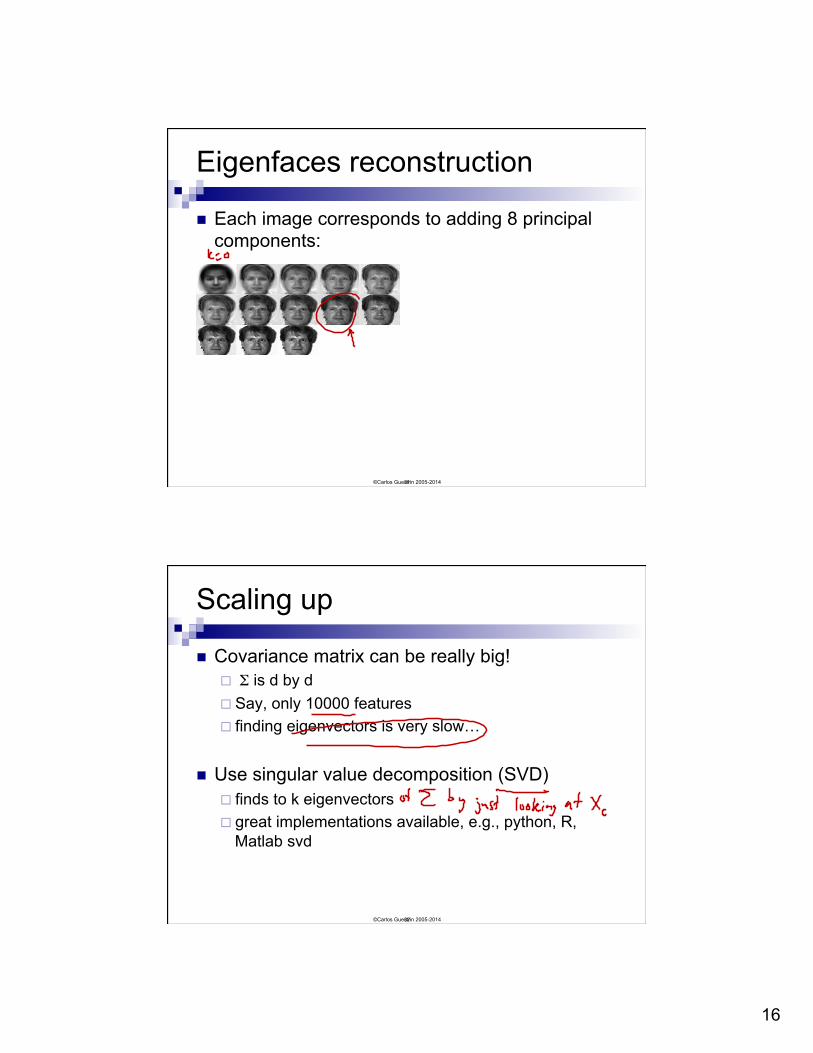
Eigenfaces reconstruction

n  Each image corresponds to adding 8 principal components:


32

Scaling up

n  Covariance matrix can be really big! ¨  Σ is d by d ¨ Say, only 10000 features ¨  finding eigenvectors is very slow…

n  Use singular value decomposition (SVD) ¨  finds to k eigenvectors ¨ great implementations available, e.g., python, R,

Matlab svd


17

33

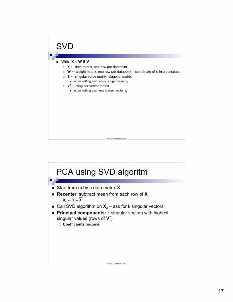
SVD n  Write X = W S VT

¨  X ← data matrix, one row per datapoint ¨  W ← weight matrix, one row per datapoint – coordinate of xi in eigenspace ¨  S ← singular value matrix, diagonal matrix

n  in our setting each entry is eigenvalue λj ¨  VT ← singular vector matrix

n  in our setting each row is eigenvector vj


34

PCA using SVD algoritm

n  Start from m by n data matrix X n  Recenter: subtract mean from each row of X

¨  Xc ← X – X n  Call SVD algorithm on Xc – ask for k singular vectors

n  Principal components: k singular vectors with highest singular values (rows of VT) ¨  Coefficients become:


18

35

What you need to know

n  Dimensionality reduction ¨ why and when it’s important

n  Simple feature selection n  Principal component analysis

¨ minimizing reconstruction error ¨  relationship to covariance matrix and eigenvectors ¨ using SVD


expectation maximization - university of washington

Documents