1

Experiment 0 Matlab and LabJack Programming Exercise

I. Purpose

The main purpose of this exercise is to give you an introduction to using Matlab for controlling equipment and collecting data, and making decent plots.

II. Equipment

optical breadboard LabJack interface diode laser motor controller amplified photodiode stepper motor computer with Matlab translation stage

III. Introduction

In Physics 375, you will be collecting and analyzing your data using Matlab. You can write general purpose programs in Matlab, much like you would in Mathematica or using C or any other programming language. Matlab is widely used in science and engineering because it is particularly good at numerical calculations. It is also possible to use Matlab programs to control or collect data from other electronic equipment, although this is much less commonly done than using it for numerical work.

In this lab, you will first work through a brief introduction to Matlab. Matlab is a powerful   programming   environment.   Although   you   can’t   learn   everything   about   Matlab   in   a  semester,  and  this  really  isn’t  a  course  about Matlab, we will try to acquaint you with the bare essentials. By the end of this exercise, you will use a Matlab routine to read analog voltages from   a   data   acquisition   unit   (“LabJack”)   through   a USB connection and record the optical intensity of a laser with a photodiode – an operation we will be using for the experiments in PHYS375 over and over again throughout this semester.

IV. ExperimentPART A: Introduction to Matlab Set up your working area - It will be useful to have an area on your computer where you can store useful code and your

data from experiments. You will find some code snippets on the PHYS 375 course website, which is linked at http://umdphysics.umd.edu/academics/courses. There you should find several files:

data.dat 02-Feb-2012 08:53 1k lj_get.m 02-Feb-2012 08:53 1k lj_step.m 02-Feb-2012 08:53 1k ...

2

Right-click on the first of  the  files  and  choose  “save  target  as”.       On   the   left,   choose   “Local  Disk   (C   :)”     then   “Users”   then   an   area   that   has   a   name   similar   to  “p375-08”  then  “My  Documents”  then  “Matlab”.    

At this point, look towards the top left of the window and  choose   “New  Folder”   and   create   a  folder with your full name (first and last). Save this file and then do the same for the other files in the codes and snippets folder. For the rest of the class, put all the other files that you create during the lab in this folder that you have created.

STARTING MATLAB

Find the Matlab Icon on the desktop and double click on it. After Matlab starts up, it will open one or more windows.

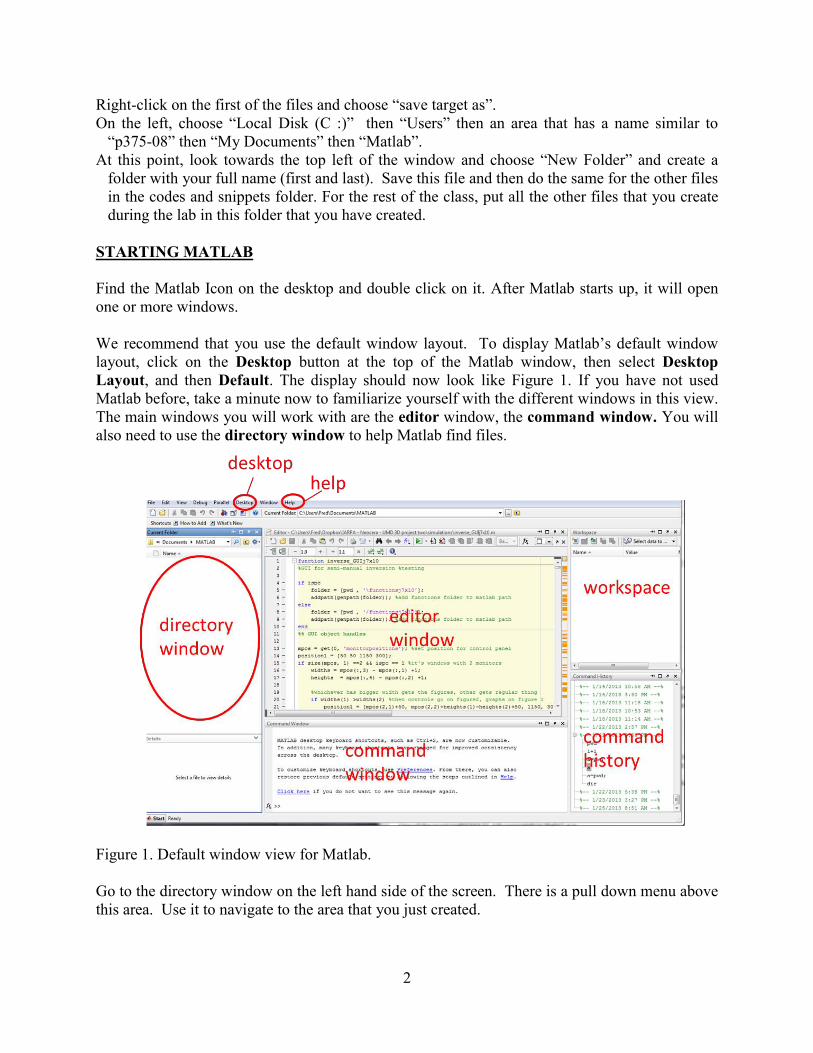
We recommend that you use the default window layout. To  display  Matlab’s  default  window  layout, click on the Desktop button at the top of the Matlab window, then select Desktop Layout, and then Default. The display should now look like Figure 1. If you have not used Matlab before, take a minute now to familiarize yourself with the different windows in this view. The main windows you will work with are the editor window, the command window. You will also need to use the directory window to help Matlab find files.

Figure 1. Default window view for Matlab.

Go to the directory window on the left hand side of the screen. There is a pull down menu above this area. Use it to navigate to the area that you just created.

3

USING MATLAB Take a look at the command window. You should see >> at the bottom of the command window.  This   is  Matlab’s   prompt   and   it  means   it   is   ready   and  waiting to accept a command. Matlab has a huge number of commands and functions. Try typing into the command window 1+2 and then hit Enter >> 1+2 ans = 3 Matlab calculates the answer, assigns it to the variable ans, and then displays the result. Next try typing ans and hit Enter: >> ans ans = 3 You can see that Matlab simply reported the value of that variable. Assigning values to variables You can also have Matlab assign values to variables that you define. Try entering the following on one line: >> a=4; b=6; In this case, Matlab just responds with a prompt sign and no other output. The semicolon is used to suppress output and lets you put multiple commands on the same line. Now enter a*b and Matlab should respond with: >> a*b ans = 24 Now try entering a=a+1 : >> a=a+1 a = 5 Of course, a = a+1 cannot be true for any real number a. The = in Matlab does not mean equals in the usual mathematical sense. Rather = means assign the variable on the left (a in this case) the value given by performing the operations on the right (in this case adding 1 to the starting value for a, which is 4 since you defined it to be 4 earlier). Standard functions Many familiar functions work in Matlab. For example try entering the following examples: pi sqrt(9) 3^3 factorial(4) cos(pi) sin(pi) tanh(1) exp(1) log10(100) log(2.71828) Note that Matlab is case-sensitive and all built-in functions we will be using are lowercase. Even though Matlab normally displays only a limited number of significant digits, it stores values with higher precision. You can switch it between higher- and lower-precision displays by typing format long or format short .

4

When you are starting out, one of the most useful Matlab commands is help. Try typing help into the command window and get everything, or type help and the name of a function to find out about a specific function. For example: >> help exp You can also use help to discover  other  related  functions  that  might  be  helpful  as  well  in  the  “See  also”  section  in  the  output  from  the  “help”  command. Your working directory In addition to executing commands, Matlab can also execute Matlab programs or scripts that are saved as files. To run a Matlab routine, you need to let Matlab know where the files are. You can see where Matlab is looking for files by typing pwd (for print working directory) in the command window: >> pwd ans = C:\DocumentsandSettings\ian\MyDocuments\Matlab All the usual MSDOS and Linux commands for directory manipulations are available. For instance, try the following commands: >> cd .. >> dir >> ls The command cd changes your working directory, and cd followed by two dots changes it to the next higher level or folder. dir (short for directory) or ls (shorthand for list) tells you the files in your working area. You should see the area you created there. Go back into your working area by typing: >> cd ’your area name’ You don’t  need  those  quotes unless your directory name contains a space. Note that these are single-quote marks, not double-quotes. Another way to change to your directory, even if it contains a space in the name, is to type cd followed by the first few letters of the directory name and then hit the tab key for completion. Once you are back in your directory, see what is in it: >> dir MATRICES AND ARRAYS From  the  Matlab  “Getting  Started”  Guide (http://www.mathworks.com/access/helpdesk/help/pdf_doc/matlab/getstart.pdf): “In the Matlab environment, a matrix is a rectangular array of numbers. Special meaning is sometimes attached to 1-by-1 matrices, which are scalars, and to matrices with only one row or column, which are vectors. Matlab has other ways of storing both numeric and nonnumeric data, but in the beginning, it is usually best to think of everything as a matrix. The operations in Matlab are designed to be as natural as possible. Where other programming languages work with numbers one at a time, Matlab allows you to work with entire matrices quickly and easily.”  In fact the Mat in Matlab stands for matrices.

5

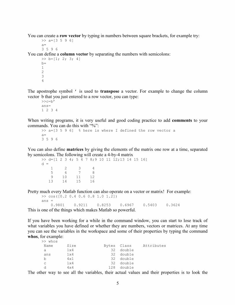
You can create a row vector by typing in numbers between square brackets, for example try: >> a=[3 5 9 6] a= 3 5 9 6 You can define a column vector by separating the numbers with semicolons: >> b=[1; 2; 3; 4] b= 1 2 3 4 The apostrophe symbol ’ is used to transpose a vector. For example to change the column vector b that you just entered to a row vector, you can type: >>c=b’ ans= 1 2 3 4 When writing programs, it is very useful and good coding practice to add comments to your commands.  You  can  do  this  with  “%”:   >> a=[3 5 9 6] % here is where I defined the row vector a a= 3 5 9 6 You can also define matrices by giving the elements of the matrix one row at a time, separated by semicolons. The following will create a 4-by-4 matrix >> d=[1 2 3 4; 5 6 7 8;9 10 11 12;13 14 15 16] d = 1 2 3 4 5 6 7 8 9 10 11 12 13 14 15 16 Pretty much every Matlab function can also operate on a vector or matrix! For example: >> cos([0.2 0.4 0.6 0.8 1.0 1.2]) ans = 0.9801 0.9211 0.8253 0.6967 0.5403 0.3624 This is one of the things which makes Matlab so powerful. If you have been working for a while in the command window, you can start to lose track of what variables you have defined or whether they are numbers, vectors or matrices. At any time you can see the variables in the workspace and some of their properties by typing the command whos, for example: >> whos Name Size Bytes Class Attributes a 1x4 32 double ans 1x4 32 double b 4x1 32 double c 1x4 32 double d 4x4 128 double The other way to see all the variables, their actual values and their properties is to look the

6

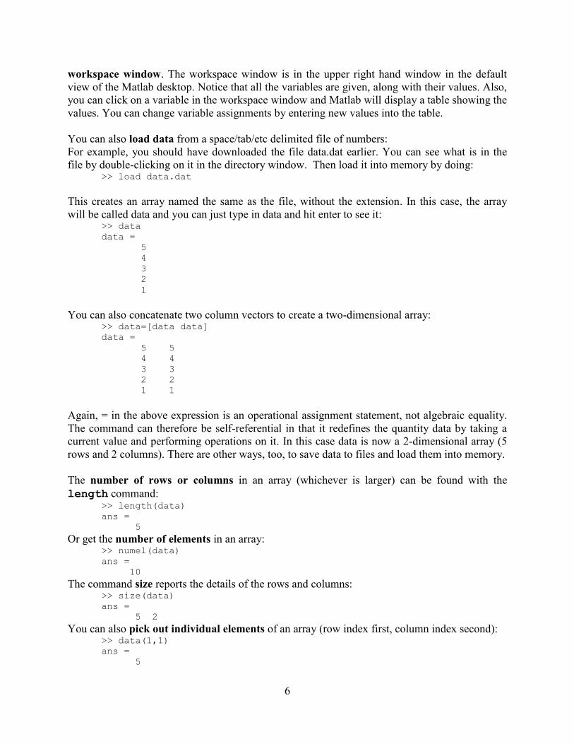
workspace window. The workspace window is in the upper right hand window in the default view of the Matlab desktop. Notice that all the variables are given, along with their values. Also, you can click on a variable in the workspace window and Matlab will display a table showing the values. You can change variable assignments by entering new values into the table. You can also load data from a space/tab/etc delimited file of numbers: For example, you should have downloaded the file data.dat earlier. You can see what is in the file by double-clicking on it in the directory window. Then load it into memory by doing: >> load data.dat This creates an array named the same as the file, without the extension. In this case, the array will be called data and you can just type in data and hit enter to see it: >> data data = 5 4 3 2 1 You can also concatenate two column vectors to create a two-dimensional array: >> data=[data data] data = 5 5 4 4 3 3 2 2 1 1 Again, = in the above expression is an operational assignment statement, not algebraic equality. The command can therefore be self-referential in that it redefines the quantity data by taking a current value and performing operations on it. In this case data is now a 2-dimensional array (5 rows and 2 columns). There are other ways, too, to save data to files and load them into memory. The number of rows or columns in an array (whichever is larger) can be found with the length command: >> length(data) ans = 5 Or get the number of elements in an array: >> numel(data) ans = 10 The command size reports the details of the rows and columns: >> size(data) ans = 5 2 You can also pick out individual elements of an array (row index first, column index second): >> data(1,1) ans = 5

7

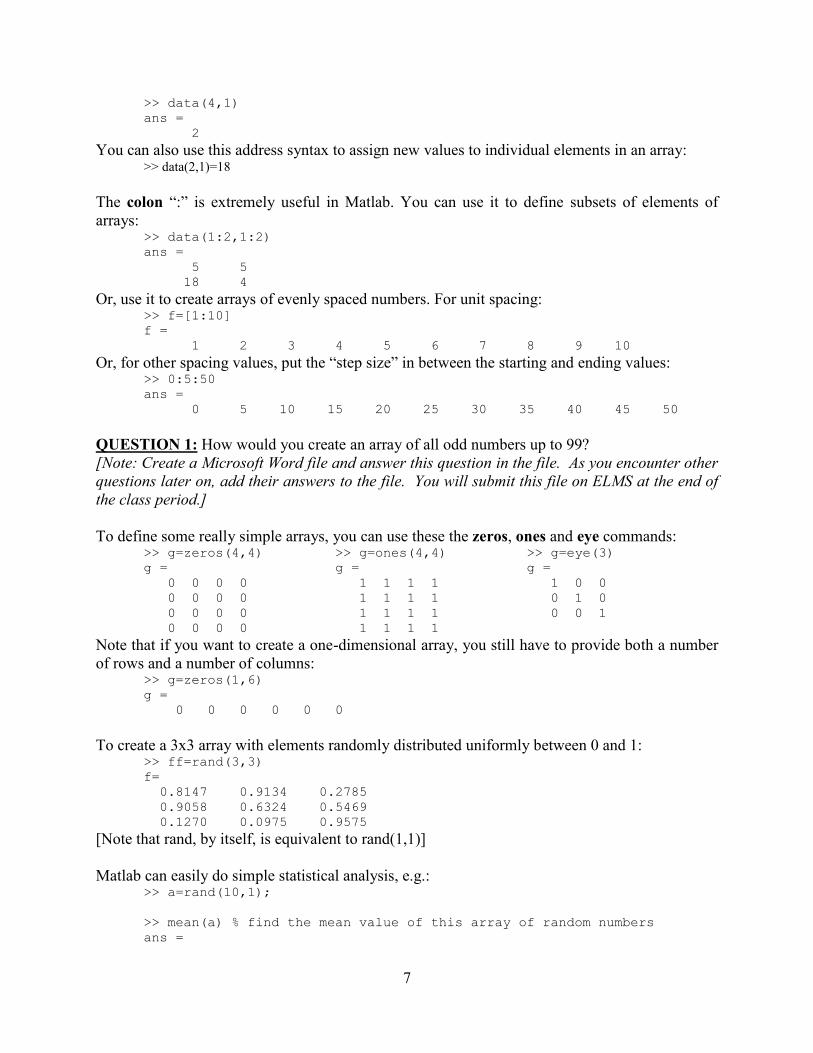
>> data(4,1) ans = 2 You can also use this address syntax to assign new values to individual elements in an array: >> data(2,1)=18 The colon “:”   is   extremely   useful   in  Matlab.  You   can   use   it   to   define   subsets of elements of arrays: >> data(1:2,1:2) ans = 5 5 18 4 Or, use it to create arrays of evenly spaced numbers. For unit spacing: >> f=[1:10] f = 1 2 3 4 5 6 7 8 9 10 Or, for other spacing values, put the  “step  size”  in  between  the  starting  and  ending  values: >> 0:5:50 ans = 0 5 10 15 20 25 30 35 40 45 50 QUESTION 1: How would you create an array of all odd numbers up to 99? [Note: Create a Microsoft Word file and answer this question in the file. As you encounter other questions later on, add their answers to the file. You will submit this file on ELMS at the end of the class period.] To define some really simple arrays, you can use these the zeros, ones and eye commands: >> g=zeros(4,4) >> g=ones(4,4) >> g=eye(3) g = g = g = 0 0 0 0 1 1 1 1 1 0 0 0 0 0 0 1 1 1 1 0 1 0 0 0 0 0 1 1 1 1 0 0 1 0 0 0 0 1 1 1 1 Note that if you want to create a one-dimensional array, you still have to provide both a number of rows and a number of columns: >> g=zeros(1,6) g = 0 0 0 0 0 0 To create a 3x3 array with elements randomly distributed uniformly between 0 and 1: >> ff=rand(3,3) f= 0.8147 0.9134 0.2785 0.9058 0.6324 0.5469 0.1270 0.0975 0.9575 [Note that rand, by itself, is equivalent to rand(1,1)] Matlab can easily do simple statistical analysis, e.g.: >> a=rand(10,1); >> mean(a) % find the mean value of this array of random numbers ans =

8

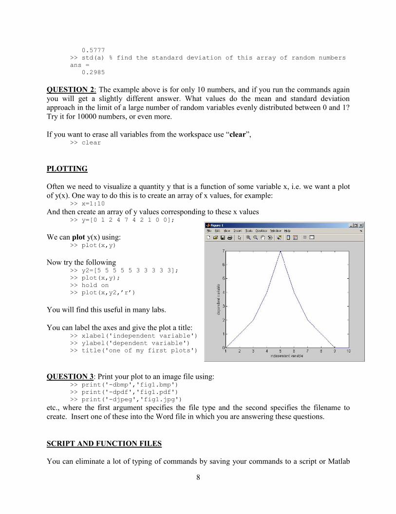
0.5777 >> std(a) % find the standard deviation of this array of random numbers ans = 0.2985 QUESTION 2: The example above is for only 10 numbers, and if you run the commands again you will get a slightly different answer. What values do the mean and standard deviation approach in the limit of a large number of random variables evenly distributed between 0 and 1? Try it for 10000 numbers, or even more. If  you  want  to  erase  all  variables  from  the  workspace  use  “clear”,   >> clear PLOTTING Often we need to visualize a quantity y that is a function of some variable x, i.e. we want a plot of y(x). One way to do this is to create an array of x values, for example: >> x=1:10 And then create an array of y values corresponding to these x values >> y=[0 1 2 4 7 4 2 1 0 0]; We can plot y(x) using: >> plot(x,y) Now try the following >> y2=[5 5 5 5 5 3 3 3 3 3]; >> plot(x,y); >> hold on >>  plot(x,y2,’r’) You will find this useful in many labs. You can label the axes and give the plot a title: >> xlabel('independent variable') >> ylabel('dependent variable') >> title('one of my first plots') QUESTION 3: Print your plot to an image file using: >> print('-dbmp','fig1.bmp') >> print('-dpdf','fig1.pdf') >> print('-djpeg','fig1.jpg') etc., where the first argument specifies the file type and the second specifies the filename to create. Insert one of these into the Word file in which you are answering these questions. SCRIPT AND FUNCTION FILES You can eliminate a lot of typing of commands by saving your commands to a script or Matlab

9

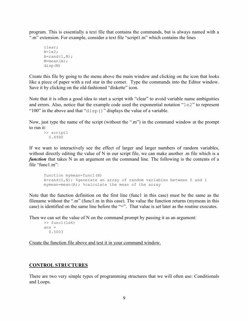
program. This is essentially a text file that contains the commands, but is always named with a “.m”  extension.  For  example,  consider  a  text  file  “script1.m”  which  contains  the  lines   clear; N=1e2; A=rand(1,N); M=mean(A); disp(M) Create this file by going to the menu above the main window and clicking on the icon that looks like a piece of paper with a red star in the corner. Type the commands into the Editor window. Save it by clicking on the old-fashioned  “diskette”  icon.   Note that it is often a good idea to start a script  with  “clear”  to  avoid  variable name ambiguities and errors. Also, notice that the example code used  the  exponential  notation  “1e2”  to  represent  “100”  in  the  above  and  that  “disp()”  displays  the  value  of  a  variable. Now,  just  type  the  name  of  the  script  (without  the  “.m”)  in the command window at the prompt to run it: >> script1 0.4990 If we want to interactively see the effect of larger and larger numbers of random variables, without directly editing the value of N in our script file, we can make another .m file which is a function that takes N as an argument on the command line. The following is the contents of a file “func1.m”: function mymean=func1(N) A=rand(1,N); %generate an array of random variables between 0 and 1 mymean=mean(A); %calculate the mean of the array Note that the function definition on the first line (func1 in this case) must be the same as the filename  without  the  “.m” (func1.m in this case). The value the function returns (mymean in this case) is identified on the same line before  the  “=”. That value is set later as the routine executes. Then we can set the value of N on the command prompt by passing it as an argument: >> func1(1e6) ans = 0.5003 Create the function file above and test it in your command window. CONTROL STRUCTURES There are two very simple types of programming structures that we will often use: Conditionals and Loops.

10

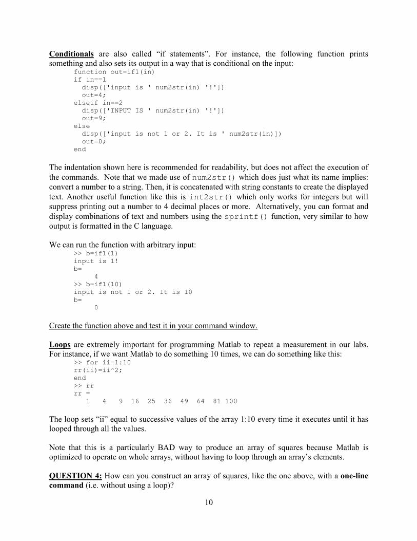
Conditionals are   also   called   “if   statements”.   For   instance,   the   following   function   prints  something and also sets its output in a way that is conditional on the input: function out=if1(in) if in==1 disp(['input is ' num2str(in) '!']) out=4; elseif in==2 disp(['INPUT IS ' num2str(in) '!']) out=9; else disp(['input is not 1 or 2. It is ' num2str(in)]) out=0; end The indentation shown here is recommended for readability, but does not affect the execution of the commands. Note that we made use of num2str() which does just what its name implies: convert a number to a string. Then, it is concatenated with string constants to create the displayed text. Another useful function like this is int2str() which only works for integers but will suppress printing out a number to 4 decimal places or more. Alternatively, you can format and display combinations of text and numbers using the sprintf() function, very similar to how output is formatted in the C language. We can run the function with arbitrary input: >> b=if1(1) input is 1! b= 4 >> b=if1(10) input is not 1 or 2. It is 10 b= 0 Create the function above and test it in your command window. Loops are extremely important for programming Matlab to repeat a measurement in our labs. For instance, if we want Matlab to do something 10 times, we can do something like this: >> for ii=1:10 rr(ii)=ii^2; end >> rr rr = 1 4 9 16 25 36 49 64 81 100 The  loop  sets  “ii”  equal  to  successive  values  of  the  array  1:10  every  time  it  executes  until  it  has  looped through all the values. Note that this is a particularly BAD way to produce an array of squares because Matlab is optimized to operate on whole arrays, without having to loop through  an  array’s  elements. QUESTION 4: How can you construct an array of squares, like the one above, with a one-line command (i.e. without using a loop)?

11

There are other types of loops. For instance, ii=1; while rand<0.9 ii=ii+1; end disp(ii) This loop  will   execute   the   code   before   the   “end”   statement   and   increment   “ii”   by   1   until   the  random number generated by  “rand”  is  equal  to  or  more  than  0.9.  Once  it  satisfies  this  constraint,  it will display the number of loop iterations. QUESTION 5: What is the mean value of ii after this code executes a large number of times? Write a function and a script which calls the function to determine this. Also insert the function code and script code into your Word document along with your answer to the question. Note that it is possible to write code for a loop (intentionally, or by mistake) which will never end because the  “while”  statement  is  always  satisfied. If your code gets into an infinite loop, you can stop it by pressing control-c. PART B: Indentify the main parts of the apparatus Now that you have had some practice working with Matlab, it is time to get it to do something useful like control a motor and collect some data. Take a look at the setup and identify the major pieces of equipment:

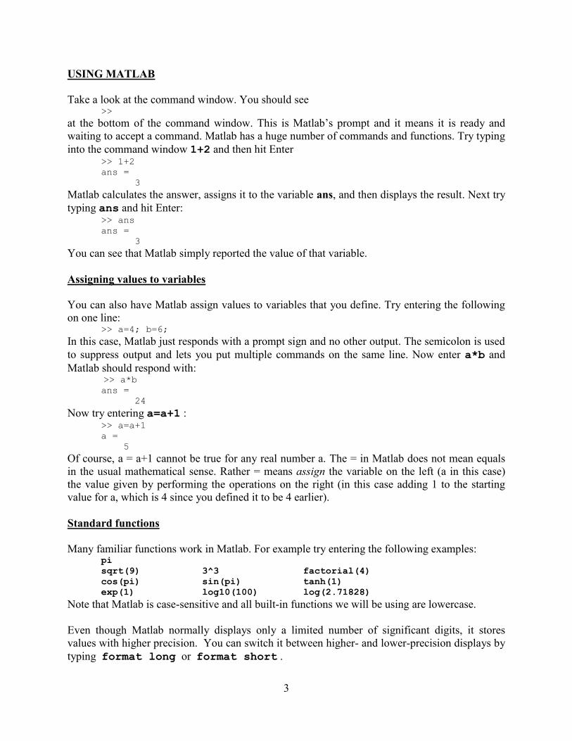
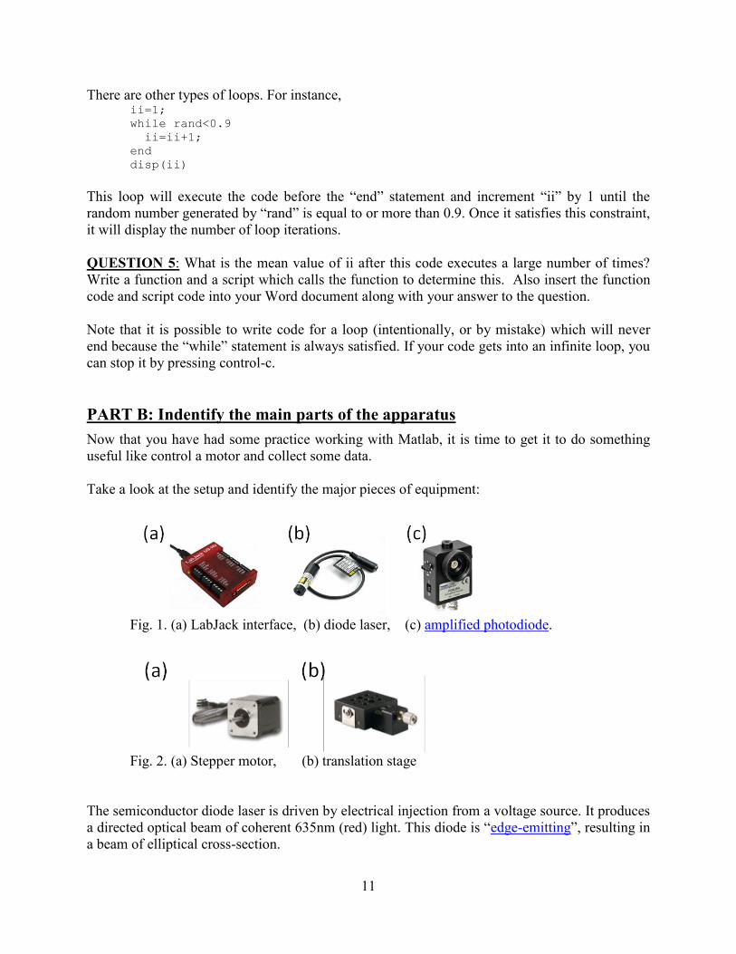
Fig. 1. (a) LabJack interface, (b) diode laser, (c) amplified photodiode.

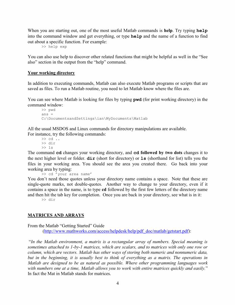
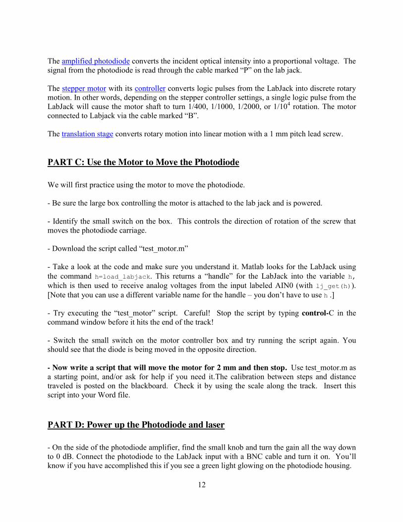
Fig. 2. (a) Stepper motor, (b) translation stage

The semiconductor diode laser is driven by electrical injection from a voltage source. It produces a  directed  optical  beam  of  coherent  635nm  (red)  light.  This  diode  is  “edge-emitting”,  resulting  in  a beam of elliptical cross-section.

12

The amplified photodiode converts the incident optical intensity into a proportional voltage. The signal from the photodiode  is  read  through  the  cable  marked  “P”  on  the  lab  jack. The stepper motor with its controller converts logic pulses from the LabJack into discrete rotary motion. In other words, depending on the stepper controller settings, a single logic pulse from the LabJack will cause the motor shaft to turn 1/400, 1/1000, 1/2000, or 1/104 rotation. The motor connected to Labjack  via  the  cable  marked  “B”. The translation stage converts rotary motion into linear motion with a 1 mm pitch lead screw. PART C: Use the Motor to Move the Photodiode We will first practice using the motor to move the photodiode. - Be sure the large box controlling the motor is attached to the lab jack and is powered. - Identify the small switch on the box. This controls the direction of rotation of the screw that moves the photodiode carriage. - Download the script  called  “test_motor.m”   - Take a look at the code and make sure you understand it. Matlab looks for the LabJack using the command h=load_labjack.   This   returns   a   “handle”   for   the   LabJack   into   the   variable   h, which is then used to receive analog voltages from the input labeled AIN0 (with lj_get(h)). [Note that you can use a different variable name for the handle – you  don’t  have  to  use h .] - Try   executing   the   “test_motor”   script.    Careful! Stop the script by typing control-C in the command window before it hits the end of the track! - Switch the small switch on the motor controller box and try running the script again. You should see that the diode is being moved in the opposite direction. - Now write a script that will move the motor for 2 mm and then stop. Use test_motor.m as a starting point, and/or ask for help if you need it.The calibration between steps and distance traveled is posted on the blackboard. Check it by using the scale along the track. Insert this script into your Word file. PART D: Power up the Photodiode and laser - On the side of the photodiode amplifier, find the small knob and turn the gain all the way down to 0 dB. Connect the photodiode to the LabJack input with a BNC cable and turn it on. You’ll know if you have accomplished this if you see a green light glowing on the photodiode housing.

13

- After securely mounting your laser, turn it on by plugging it in. Please be very careful with the laser! If shined directly into your eyes, it could permanently damage your retina! Be sure to also watch out for stray reflections from the photodiode and other things that the laser beam hits! Use the thumbscrews on the laser mount to align the laser beam level with the breadboard. The upper screw controls the vertical while the lower controls the horizontal position. Also, there is a screw that can be used to do coarse adjustments to the height on the holder that is used to mount the laser carriage onto the optical bread board. - Align the photodiode and the laser. Be sure the photodiode track is parallel to the optical board. - Download the script test_photodiode.m and modify it so that it measures the voltage from the photodiode every 0.05 seconds (type help pause for an explanation of the pause function) - Run your modified version of test_photodiode.m and use it to align the laser with the diode and aperture by maximizing the signal in real time. You may notice that the voltage is always below ~10V, which is the LabJack input limit; it has an input range of -10V to +10V. You may also notice that even without adjusting the alignment, the voltage fluctuates between 2 or more exact voltages. This is because the Labjack discretizes the input voltage from the photodiode using a 12-bit analog-to-digital converter and does not have unlimited resolution. What happens when you open and close the aperture, or pass your hand in front of the photodiode? If you turn off the laser, is the photodiode voltage zero? Why or why not? PART E: Mapping the Profile of the Laser Beam

Assuming that you’ve gotten to this point and still have time left, do some useful things with the tools  you’ve  learned!    Place the translation stage at some chosen distance from the laser and map the profile of the laser beam by moving the photodiode across it with the motor drive, recording the voltage as you go. Store the measured voltages in an array, plot the voltage vs. position, and also save the voltages to a file. (Hint: you can use the save command.) Now move the translation stage to a significantly different distance from the laser and map the profile there. Plot both profiles together, making your plot professional-looking by adding an appropriate title and axis labels, plus a legend. Consult the online help and/or ask us for help or advice if you need it. Insert this plot into the Word file with the questions you’ve been answering. PART F: Finishing Up

At this point you should have a Word file with your answers to the numbered questions in part A, the scripts that you wrote in a few specified places, and some plots. Before leaving the lab, submit this file to ELMS Canvas. This will be your record of work done in the lab today and will contribute some to your grade (though not as much as the lab reports you’ll write later).