experiment 11 pulses in transmission lines

Revised 9/2006.

Copyright © 2006 The Board of Trustees of the University of Illinois. All rights reserved.

University of Illinois at Urbana-Champaign Department of Physics Physics 401 Classical Physics Laboratory

Experiment 11

Pulses in Transmission Lines

Table of Contents

I. Introduction--------------------------------------------------------------------------------------------2

II. The Differential Equations for an Ideal Line------------------------------------------------------2

III. Characteristic Impedance----------------------------------------------------------------------------4

IV. Reflection of Pulses at Resistances-----------------------------------------------------------------7

V. The Thevenin Equivalent Circuit of a Line------------------------------------------------------10

VI. More Complicated Circuits at the End of the Line--------------------------------------------- 10

VII. Exercises--------------------------------------------------------------------------------------------- 12

A. Speed of waves on RG8U and RG58U------------------------------------------------- 13

B. Resistive termination---------------------------------------------------------------------- 14

C. Thevenin's theorem------------------------------------------------------------------------ 14

D. Capacitor at the end of the line-----------------------------------------------------------15

E. Inductor at the end of the line------------------------------------------------------------ 16

F. LC circuit------------------------------------------------------------------------------------17

G. Unknown------------------------------------------------------------------------------------17

VIII. Report-------------------------------------------------------------------------------------------------17

Appendix I. Characteristics of parallel and coaxial conductor transmission lines------------------ 18

Appendix II. Adjustment of oscilloscope probe--------------------------------------------------------- 19

Appendix III. Production of pulses with cable and switch--------------------------------------------- 21

Physics 401 Expt 11 2/23 Pulses in Transmission Lines

I. Introduction In the discussion of the transient response of the RLC circuit to step voltages, we have ignored the time required for the signal to propagate to the various circuit elements. This neglect is justified for those cases where the time scale involved in the circuit is much greater than that involved in the propagation of signals along the wires. This neglect is not possible if the propagation times times are of the order of nanoseconds ( 910− s), since the maximum velocity with which a signal can be propagated is that of light, 30 cm per ns. Although we must allow for the complications of these time delays in ordinary circuits at radio frequencies, it is difficult to treat such a general system theoretically. We will, however, try to understand the propagation of signals in a simple circuit: a uniform two-conductor transmission line. The propagation of signals in these lines is described by two parameters: the propagation speed and the characteristic impedance. In turn these two parameters are related to the capacitance and inductance per unit length of the line. We will consider only the special case of a lossless line, for which the series resistance and the shunt conductance are negligible. In this approximation the signal is transmitted without attenuation, although distortion can still result from variation of the dielectric constant with frequency. This approximaton is useful for short lines and cables used in transmitting signals no more than a few meters. In transmission lines more than 30 meters long, the distortion and attenuation of signals in the line are sometimes a major problem and must be considered in detail. These effects are discussed briefly in a later section. II. The differential equations for an ideal line A uniform ideal line can be described by its series inductance L per unit length and its shunt capacitance C per unit length. If such a line is connected to a voltage generator, currents will flow along the line through the series inductance, and the currents will charge the shunt capacitance. Differential equations for the voltage V and current i at a point x on the line are derived as follows. (Note that V and i are functions of both x and t). The voltage dV across an element of length dx (see Fig. 1) is determined by the series inductance Ldx and is given by


( ) didV L dxdt

= − , or dV diLdx dt

= − .

Fig. 1 Voltage and current in an ideal line. Since V and i are functions of the two variables x and t, this equation is expressed in terms of partial derivatives,

i x tV L∂ ∂

∂ ∂= − . (1)

Similarly, the current is reduced by an amount di in an element of length dx because of the charging of the shunt capacitance Cdx, so that

( ) dVdi C dxdt

= − , or di dVCdx dt

= −

In terms of partial derivatives

i VCx t

∂ ∂= −∂ ∂

. (2)

Eqs. 1 and 2 can be combined to obtain wave equations for V and i. Differentiate Eq. 1 with respect to x, we obtain

2 2

2

V iLt xx

∂ ∂= −∂ ∂∂

, (3)


and differentiating Eq. 2 with respect to t, we obtain

2 2

2

i VCx t t

∂ ∂= −∂ ∂ ∂

. (4)

Since we are dealing with differentials of well behaved functions,

2 2

t x x t∂ ∂=

∂ ∂ ∂ ∂,

and Eqs. 3 and 4 combine to give the wave equation for V,

2 2

2 2

V VLCx t

∂ ∂=∂ ∂

. (5)

Similarly, by differentiating Eq. 1 with respect to t and Eq. 2 with respect to x, we obtain a wave equation for i,

2 2

2 2

i iLCx t

∂ ∂=∂ ∂

. (6)

The two wave equations Eq. 5 and Eq. 6 correspond to current and voltage waves with a propagation speed u of

1uLC

= . (7)

III. Charcteristic impedance

Consider traveling wave solutions for V and i in the +x direction at a speed 1uLC

= .

These waves must have the general mathematical forms ( ) ( ),V x t f x u t= − and ( ) ( ),i x t g x u t= − .


We will now show that these waves have the same shape, and that the voltage wave is proportional to the current wave. From Eq. 1 we have

f gLx t

∂ ∂= −∂ ∂

. (8)

Let w x ut= − , so dffdw

′ = and dggdw

′ = .

Then

gf Lt

∂′= −∂

and

'g ugt

∂ = −∂

.

Therefore, from Eq. 8,

1 Lf Lug L g gCLC

′ ′ ′ ′= − = = , or Lf gC

′ ′= . (9)

When integrated, this equation gives

constantLf gC

= + .

Any DC voltages and currents that may be on the cable are usually ignored in treatments of transmission lines; therefore the constant of integration in Eq. 9 is set to zero. Hence

Lf gC

=

and, therefore,

LV iC

= (10)


Thus the voltage and current waves have the same shape. The ratio V i is called the characteristic impedance kZ of the line. We have now shown that

kV LZi C

= = . (11)

Note that kZ is real and has the units of resistance.

To summarize, a voltage–current wave can travel toward +x with the velocity

1 LCu = . The voltage and current in this incident wave are related as i k iV Z i= . A reflected

wave pulse can travel toward -x with the velocity 1 LCu = − . The voltage and current in this wave are related as r k rV Z i= − .

At any point on the transmission line the voltage V and the current i are the sum of the voltages and currents in the positive and negative going, i.e. incident and reflected, waves. Thus r iV V V= + , and

i rr i

k k

V Vi i i

Z Z= + = − ,

or r iV V V+ = , and

(12) i r kV V Z i− = .

These two equations are very important for understanding the propagation of waves on transmission lines. Useful expressions for the propagation speed and characteristic impedance of parallel conductor and coaxial conductor transmission lines are given in the Appendix I.


IV. Reflection of pulses at resistive loads Eqs. 12 are useful for determining the kind of reflection that will occur from the end of a transmission line terminated in a resistive load. Suppose a square pulse of amplitude oV is

traveling toward +x as shown in Fig 2.

Figure 2 At the end of the line it encounters a load resistance LR . Consequently at the end of the line V

and i in Eq. 12 must be related as

LV Ri

= .

The incident wave generates a reflected wave at the load for which

i r L

i r k k

V V RVV V Z i Z

+= =

−. (13)

Solving Eq. 13 for rV gives

L kr i

L k

R ZV V

R Z−

=+

. (14)

If the incident pulse is a square pulse of magnitude i oV V= , and the line is left open (or disconnected) so that LR = ∞ , Eq. 14 gives

r iV V= , or r oV V= . (open line) (15)

Thus a pulse of equal magnitude is reflected back down the line as shown in Figure 3a. On the other hand if LR = 0, a shorted line, Eq. 14 gives


r iV V= − , or r oV V= − . (shorted line) (16)

Figure 3 This reflected pulse will have the same magnitude as the incident pulse, but it will be inverted as shown in Figure 3 (b). For a pulse traveling on a line toward +x the voltage-current relations are i i kV i Z= . Consequently a load resistance L kR Z= should behave like a continuation of the line and no pulse should be reflected. If L kR Z= in Eq. 14, we obtain 0rV = . Connecting a resistance

L kR Z= to a line is called terminating the line. Other values of LR give various sizes of

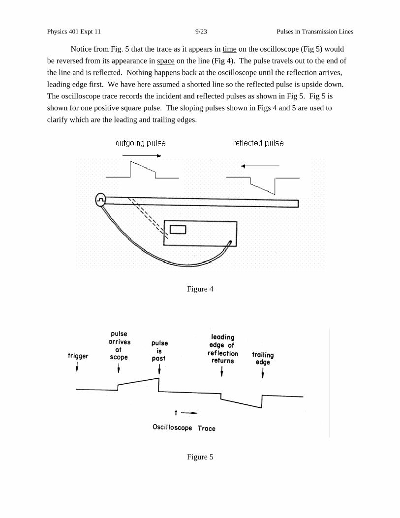
reflected pulses that can be computed from Eq. 14. Suppose an oscilloscope is connected to the line near the pulse generator as in Figure 4. On your pulse generator a trigger pulse is available that will start the sweep of the oscilloscope when the pulse is generated. As time goes on, your oscilloscope sweeps to the right as the pulse travels out on the line. Soon the leading edge of the pulse arrives at the oscilloscope and the trace jumps up and records it. As the pulse passes, the oscilloscope records its shape.


Notice from Fig. 5 that the trace as it appears in time on the oscilloscope (Fig 5) would be reversed from its appearance in space on the line (Fig 4). The pulse travels out to the end of the line and is reflected. Nothing happens back at the oscilloscope until the reflection arrives, leading edge first. We have here assumed a shorted line so the reflected pulse is upside down. The oscilloscope trace records the incident and reflected pulses as shown in Fig 5. Fig 5 is shown for one positive square pulse. The sloping pulses shown in Figs 4 and 5 are used to clarify which are the leading and trailing edges.

Figure 4

Figure 5


V. Thevenin equivalent circuit of a line Suppose a voltage pulse iV is incident on the end of a line with a resistance LR connected

to it. A reflected pulse is generated at the load. At the load Eqs. 12 may be written i r LV V R i+ = , and i r kV V Z i− = .

rV can be eliminated from these equations, and the result can be solved for i.

2 i

L

ViR Z

=+

.

The current at the load is identical to what would be obtained from the equivalent circuit shown in Fig 6.

Figure 6

Although this result was obtained on the basis of a resistance connected to the end of the line, the system is everywhere linear (i.e. currents proportional to voltages). Therefore, Thevenin's theorem applies and the line will respond to any device connected to it as if it were an emf of twice the voltage of the incoming pulse, 2 iV , being fed through an impedance equal to the characteristic impedance of the line, kZ . This fact is very important. A good many physicists

really do work every day with transmission lines propagating high-speed pulses. VI. More complicated circuits at the end of the line Suppose a capacitor LC is connected to the end of the line, which may be considered as

its Thevenin equivalent circuit shown in Fig 7.


Suppose a square pulse iV high and iT long is generated from the source and is incident

on the capacitor. From your previous experience with transient analysis you can easily determine that the voltage appearing on the capacitor will vary as a function of time as shown in Fig 8.

Figure 7

Figure 8 When Thevenin equivalent voltage 2 iV is applied, the capacitor charges up exponentially with a time constant k LZ C . When the voltage is removed, the capacitor discharges.

We now know the incident voltage, iV and the voltage at the load, LV . The first of Eqs. 12 may be solved to find the reflected voltage, r L iV V V= − , generated at the load. Fig 9a shows the incident square pulse iV . Fig 9b shows the voltage LV . Note that iV is the actual input voltage of height iV , and not the Thevenin equivalent voltage 2 iV . The voltage LV , however, does eventually rise to the Thevenin equivalent voltage 2 iV . The reflected pulse is obtained by


subtracting iV from LV as has been done graphically in Fig 9c. If this were observed with the

oscilloscope setting of Fig 4, a trace like Fig 9d would result.

Figure 9 Notice that the reflected pulse is first reflected upside down. This is because a capacitor acts like a short for rapid high frequency voltage changes. However, after a long time the reflected pulse becomes the same sign as the incident pulse. This is because the capacitor behaves like an open circuit for slow changes (DC). An inductor, on the other hand, opposes rapid changes in current and acts like an infinite impedance for rapid voltage changes or like a short for slow changes. An inductor on the line will reflect the same sign pulse to begin with and the opposite sign after some time. The time constant for the inductor is kL Z . With the inductance, L, in henries and the impedance kZ in ohms, the time constant is in seconds.

The analysis of this section can be used to find the shape of the reflected pulse for any kind of circuit connected to the line. VII. Exercises Connect the circuit shown in Fig 10. RG8U is the thick, stiff, large diameter cable. It has a characteristic impedance kZ = 50 Ω . It is made of heavy copper wire and has small losses.

Attach a BNC-T connector to the channel 1 of the Scope. Connect the 50 Ω OUTPUT of the Wavetek to one side of the BNC-T with a short piece of RG58U. Use another short RG58U


cable to connect the other side of the BNC-T to the 100’ long RG8U cable. (It is inconvenient to have the heavy RG8U cable connected directly to the Scope.) Connect the SYNC OUT of the Wavetek to external trigger of the oscilloscope. The oscilloscope is a 1M Ω input impedence, and it does not perturb the pulse which travels from the Wavetek down the long RG8U cable.

Figure 10

Set the Scope trigger to external, + slope, DC Coupling. Set the Wavetek to Fixed Duty Mode, positive unipolar pulse, 1 Volt peak amplitude, pulse period to 1 µ s. and the duty cycle

to 10 %. Record these values. Duty cycle is defined as the ratio of the on time of the pulse to the period of the pulse. Note that the pulse period is the sum of the pulse on time and pulse off time. For a pulse period of 1.0 µ s and a pulse on time of 0.1 µ s, the factor cycle is 10%.

You should now see pulses on the oscilloscope screen and their reflections. Capture an image of the Scope display to document what you see. In order to differentiate incident and reflected pulses, connect a shorted terminator (as in Fig 3) at the open end of the RG8U cable. You will observe that the reflected pulses are inverted. Capture another image of the Scope display for your notebook and report. Once you are familiar with the reflections, disconnect the shorted terminator and leave that end of the RG8U open.

A. Speed of waves on RG8U and RG58U

Measure the length of time it takes the pulse to traverse the RG8U cable from the Scope to the end of the cable and then to reflect back to the Scope. (a) Using the given length of the RG8U, calculate the propagation speed on this cable. (b) Express the propagation speed as a


fraction of the speed of light. (c) Add 100' of RG58U (the spool of small cable). Measure the time between incident and reflected pulses. (d) Calculate the propagation speed of a pulse on RG58U. (e) Compare the propagation speed on RG8U to the propagation speed on RG58U. (f) Can you detect a small reflection from the connector between the cables? Notice that the reflected pulse now has significantly rounded corners. This effect is due to losses in the cable which are larger at higher frequencies. It would do little good to compare the D.C. resistance of the cable to the characteristic impedance, kZ , because at high frequencies

the pulse travels only on the surface of the wires (skin effect) so the actual effective impedance is far from its DC value. This impedance also varies with frequency as does the dielectric constant of the insulation in the cable. All these effects distort the shape of the pulses for long transmission cables. A detailed analysis is given in standard handbooks. We will ignore such effects here, although in some later sections you should remember that theoretically sharp spikes in reflected pulses are likely to be somewhat rounded in reality. B. Resistive termination Remove the RG58U cable spool and observe the positive reflected pulse from the open RG8U cable. Connect a shorting connector (green) to the end of the cable. As you have seen earlier, the reflected pulse will be inverted. Document the observation with an image of the Scope display (if you have done some in part A above). Remove the shorting connector. Connect the special cylindrical variable resistor. This resistor is a very special high frequency carbon potentiometer. Rotate the cylinder and note the variation in the reflection. Adjust for no reflection; remove the variable resistor and measure its resistance with a DMM. This measurement determines the characteristic impedance of the cable. Record this result. Measure the reflected pulse heights for the fixed resistors in your kit, 0, 25, 50, 100, 150, and 180 ohms. Compare your results with Eq. 14. Make a graph of the reflected pulse height and the pulse height calculated from Eq. 14. C. Thevenin’s theorem Connect a BNC-T to the end of your RG8U cable in order to measure the voltage across components at the end of the cable. Use appropriate interconnections between the coaxial connects on the cable, type U, to BNC. One BNC connector in your kit has a lead soldered to the center conductor so you can observe the pulse arriving at the end of the cable with a high impedance scope probe (Fig 11). Refer to the Appendix II for proper adjustment of the probe.


This adjustment can be crucial for valid measurements. Remember to set the proper probe attenuation ratio on the scope. Record the pulse observed at the end of the cable. Compare the amplitude of the pulse at the open end of the cable (receiving end) to the amplitude of the pulse at the end of the cable connected to the Wavetek (sending end). This procedure determines the open circuit voltage of the Thevenin equivalent circuit. Verify that the open circuit voltage is 2 iV .

Terminate your line with LR = 50 Ω . Measure the voltage at the load. Calculate the

Thevenin equivalent series resistance of the cable. Verify that it is 50 Ω . Repeat with the above procedure with another of the fixed resistors in your kit. Compare your measured voltage with what would be calculated from the circuit shown in Fig. 6.

Figure 11

D. Capacitance at end of the line Connect the capacitor in your kit to the end of the line. (The capacitor is merely in series inside its aluminum container. To connect it to ground you must also connect the shorting stub to the end). Record the incident and reflected voltage pulses at the sending end, and the voltage pulse at the end of the line itself with images of Scope display. Note the voltage and time scales of the Scope. Compare your observations to Fig. 8 and Fig 9. Measure the rise and fall times of the pulse at the load. The Scope can make this measurement. By convention the rise and fall


time measurement is the time difference between the 90% and 10% maximum height of the pulse. The 10% and 90% maximum voltages are indicated by the horizontal dashed lines in the oscilloscope display during the rise and fall time measurements as shown in Figure 12 below. (This is the same wave form as in Figure 8.) Here the incident pulse, a unipolar square wave, is long enough in duration for the signal across the capacitor to rise to its maximum 2 iV . (If the

incident pulse were shorter, the capacitor would begin to discharge before the signal reached 2 iV .) Then the measured rise time 2.20rise k LZ Cτ = . The factor 2.20 is equal ln 9. The fall time is 2.20fall k LZ Cτ = . The signal discharges to 0 V, before the next incident pulse.

Figure 12

Find rise and fall time measurements in the voltage measurement menu. Determine the value of the capacitance from the rise and fall time measurements. Compare the measured value with the value stamped on the capacitor. E. Inductor at the end of the line Repeat part D with an inductor. Record the incident and reflected voltage pulses, and the voltage pulse at the end of the line itself with images of Scope display. Note the voltage and time scales of the Scope. Make a version of Fig. 8 for an inductor. Measure the rise and fall times of the pulse at the load. Determine the value of the inductance from the rise and fall time measurements. Compare the measured value with the value stamped on the inductor.


F. LC Circuit Connect your capacitor and inductor in series at the end of the line. Record the incident and reflected voltage pulses, and the voltage pulse at the end of the line itself with images of Scope display. Identify in the pulse at the load a portion of a sinusoidal oscillation. Determine the frequency of the oscillation. Compare the observed frequency with the frequency calculated from the values of the capacitor and inductor. G. Unknown Choose an unknown circuit and record its number. Record the incident and reflected voltage pulses, and the voltage pulse at the end of the line itself with images of Scope display. The unknown contains two elements, one of which is a resistor. The elements may be in series or parallel. In your report determine, with appropriate values, what is in your box. During laboratory you may wish to speculate on what is inside and try to reproduce the appropriate wave shape from your known components and calculate both component values from your measurements. IX. Report In your report answer all the questions from the procedure part. The report should include your Scope shots of waveforms and related calculations. For the unknown components, show calculations to support your result.


Appendix I. Characteristics of parallel conductor and coaxial transmission lines Type of Line

Parallel conductor

Coaxial conductor

Quantity (units)

Wire radii a Separation of centers d

a << d

Inner radius a Outer radius b

Capacitance, C (farads per meter, F/m)

ln d

a

π ε 2 ln b

a

π ε

Inductance, L (henries per meter, H/m)

ln da

µπ

ln2

ba

µπ

Velocity = 1uLC

=

(meters per second, m/s)

1µε

1µε

Characteristic Impedance

kLZC

=

(ohms, Ω)

1 ln da

µπ ε

1 ln2

ba

µπ ε

Constants for free space

o

o

µε

= 120 π Ω

o o

1µ ε

= 83 10× m/s


Appendix II. Adjustment of the Scope probe The input impedance of the Scope is not purely resistive. Its input has a capacitive component of approximately 13 pF. The Scope probe is an RC circuit, and the capacitor in this circuit can be adjusted so that the combination of the RC circuit at the input of the Scope and the RC circuit of the probe is frequency independent. The figure below shows the RC circuit of the probe and the RC circuit of the Scope input. With proper adjustment the Scope probe attenuates all frequencies by a factor of 10. For this reason the probe is called a X10 probe. The display can take into account this factor of 10 automatically if X10 probe is selected on the display menu.

The Scope has a square wave output on the front panel. The Scope will display sharp edges when the probe is connected to this square wave, if the probe is properly adjusted. A small screwdriver is needed to turn the adjustment screw on the variable capacitor in the probe. The probe must be properly adjusted or rise and fall time measurements in the laboratory exercises will be invalid. Techniue on probe compensation is shown (from Tektronix TDS3000 series manual).


Appendix III Production of pulses with a charged cable and switches Suppose a section of line of length o is isolated between two open switches as shown in Fig A1. A battery of voltage oV is connected to this isolated line through a high resistance HR , i.e. HR >> kZ .

Figure A1 Consequently the voltage on the line, shown in Fig A1b, is zero beyond the switches and oV

between them. The current on the line is everywhere zero, Fig A1c. If the two switches are closed simultaneously, then the line becomes continuous and Eq. 12 applies to it. Just after the switches are closed, the voltage V on the line is the pulse shown in Fig A1b and the current is zero. Eq. 12 gives r i oV V V+ =

(A1) 0i rV V− =

Solution of Eq. A1 gives 2i oV V= , 2r oV V= (A2)


Consequently the original static voltage distribution splits up into two pulses of one-half height travelling in opposite directions as shown in Fig A2.

Figure A2 It is obviously impossible to close two mechanical switches within a nanosecond of each other, although it could be done electronically. Using a pulse generator with a single switch isolating an open line of length o (Fig A3a) will accomplish this.

In such a pulse generator a power supply is connected to it through a high resistance, so that the central wire on the charging cable is maintained at a potential oV (Fig A3b). When the switch is closed, the original static voltage distribution breaks up into two pulses of height 2oV .

One travels to the right on the transmission line. The other "travels" to the left and is immediately reflected from the open end to follow the pulse going to the right. Thus a pulse of length 2 o and height 2oV travels down the line (see Figs A3c, d, e).

A typical switch in such a pulse generator is opened and closed magnetically 60 times a second. The switch is a mercury wetted relay encapsulated in very high pressure hydrogen and should never be opened as a precaution against explosion. The liquid mercury prevents contact bounce. The high pressure gas prevents arcing. A typical pulser of this type is shown as an example in the lab. In this experiement, however, a modern 50 MHz function generator will be used to produce positive or negative rectangular pulses.


Figure A3

experiment 11 pulses in transmission lines

Documents