1

3 Lab 3: DC Motor Transfer Function Estimation by Explicit Measurement

3.1 Introduction There are two common methods for determining a plant’s transfer function. They are:

1. Measure all the physical parameters of the system used to derive the equations. Then, use those to compute the overall transfer function (Lab 3).

2. Treat the system as a black box and use: • frequency response, or • step response

methods to determine DC gain, poles, and zeros of the system (Lab 4). The following physical quantities of the DC Motor need to be measured to determine its transfer function:

• Armature resistance: Ra [ohms] • Armature inductance: La [Henries] • Torque constant: KT [N-m/amp]. Proportionality constant that relates

Torque and current. Please refer to equation 5. • Back EMF constant: Kb [volts-s/rad]. Proportionality constant that relates

Angular velocity and back electromotive force. Please refer to equation 2. • Viscous friction coefficient: B [N-m-s/rad] • Rotor moment of inertia: J [kg-m²]

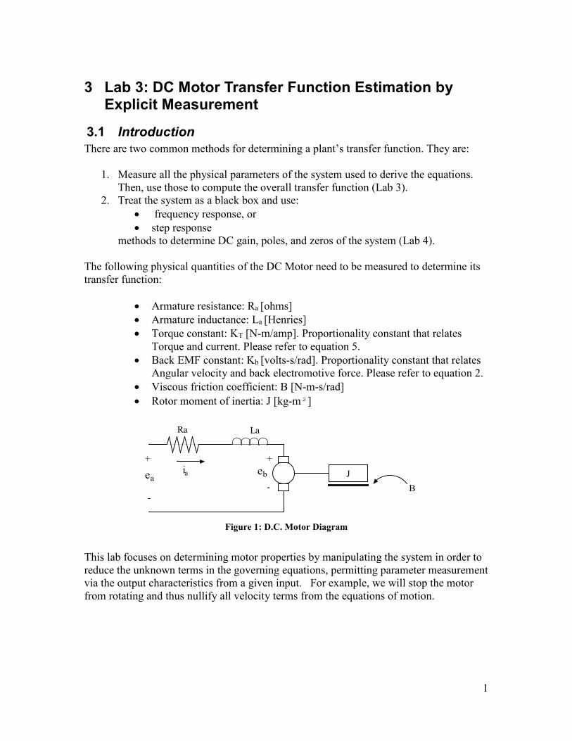
Ra La

eb

+

-J

B

iaea

+

-

Figure 1: D.C. Motor Diagram

This lab focuses on determining motor properties by manipulating the system in order to reduce the unknown terms in the governing equations, permitting parameter measurement via the output characteristics from a given input. For example, we will stop the motor from rotating and thus nullify all velocity terms from the equations of motion.

2

3.2 Pre-lab 1. In your own words, what is a mathematical model? Why are mathematical

models important in engineering? 2. Describe (with figures) two methods for determining the time constant of an

exponential decay. 3. Based on conservation of energy principals, set mechanical power equal to

electrical power and show that Kb = KT. (Use SI units for all your calculations). The easiest way to do this is to think of the situation where the positive and negative leads of the motor are shorted together (ea = 0). In this case, if you manually move the motor the only voltage generated in the circuit is due to the back-EMF of the motor. Recall that in this case, Pel = EB * IA and Pmech = Tm * ω.

4. Write the 4 electrical and mechanical equations that may be used to find the transfer function of the DC motor ω(s)/Ea(s). You should use Figure 1, the equations provided in the lab, and the example reference in Section 3.4 of the lab manual as a guide.

5. Using the equations you derived in question 4, describe how you would measure: a. Viscous friction b. Rotor moment of inertia c. Armature resistance

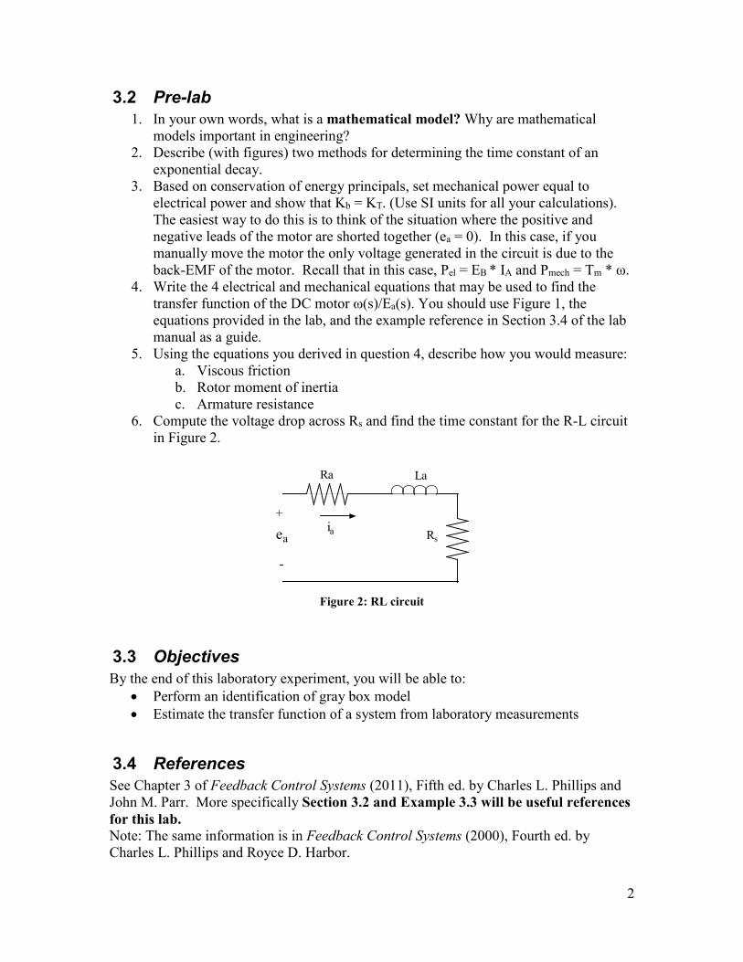
6. Compute the voltage drop across Rs and find the time constant for the R-L circuit in Figure 2.

Ra La

iaea

+

-

Rs

Figure 2: RL circuit

3.3 Objectives By the end of this laboratory experiment, you will be able to:

• Perform an identification of gray box model • Estimate the transfer function of a system from laboratory measurements

3.4 References See Chapter 3 of Feedback Control Systems (2011), Fifth ed. by Charles L. Phillips and John M. Parr. More specifically Section 3.2 and Example 3.3 will be useful references for this lab. Note: The same information is in Feedback Control Systems (2000), Fourth ed. by Charles L. Phillips and Royce D. Harbor.

3

3.5 Armature Resistance: Ra

Note: Many of the values obtained in this lab will need to be recorded and saved for future use. Please record all coefficient and parameter values on your data sheet and in a location, that you can reference during future labs.

Equation 1: Motor Circuit Voltage Equation

)()()()( tedt

tidLRtite ba

aaaa ++=

Equation 2: Angular Velocity - Back EMF

dttdKte bb)()( θ

=

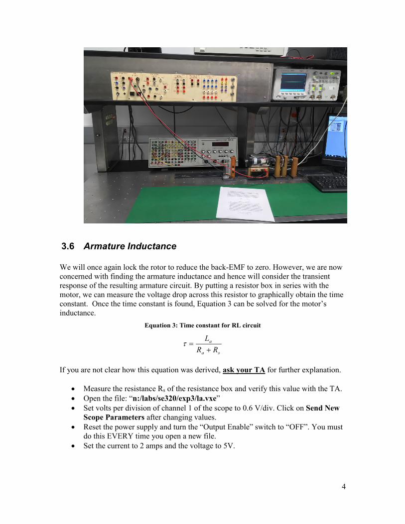
Equation 1 describes the relationship between the input voltage, ea(t), the armature resistance, Ra, armature inductance, La, and the back-EMF voltage, eb(t). If the rotor is restricted from rotating (see Figure 3), the back-EMF will become zero. This is due to the fact that back-EMF is proportional to angular velocity. Similarly, the armature inductance term will reduce to zero once steady state conditions have been reached. Hence, by measuring the input voltage and the resultant current we can measure Ra. Follow the directions below:

ea

+

-

Ra La

ia

Figure 3: Model of locked motor

• Connect the motor, flywheel and rotor locking device. Connect the HP 0-20V power supply to the motor as shown in figure below.

• Turn on all the equipment (don’t forget the HP 6632A programmable power supply) and then open the Agilent VEE file: “n:/labs/se320/exp3/ra.vxe”

• From the computer, “Reset” the power supply and then switch “Output Enable” off. Set the current to 2 amps and the voltage to 5V. The DC power supply is set to constant voltage mode and hence it will maintain the set voltage to the motor for any required amperage up to a MAXIMUM of 2 amps.

• At the Agilent VEE console, toggle the “Output Enable” of the power supply to “ON”. This enables the power supply’s voltage. You can look at the power supply’s display and see what actual voltage and current is being applied. Increment the applied voltage in steps of 0.5V until the power supply voltage is 7V, and record the values obtained at each step in your data sheet.

• Toggle “Output Enable” to “OFF” on the power supply console and show your measurements to the TA.

4

3.6 Armature Inductance We will once again lock the rotor to reduce the back-EMF to zero. However, we are now concerned with finding the armature inductance and hence will consider the transient response of the resulting armature circuit. By putting a resistor box in series with the motor, we can measure the voltage drop across this resistor to graphically obtain the time constant. Once the time constant is found, Equation 3 can be solved for the motor’s inductance.

Equation 3: Time constant for RL circuit

sa

a

RRL+

=τ

If you are not clear how this equation was derived, ask your TA for further explanation.

• Measure the resistance Rs of the resistance box and verify this value with the TA. • Open the file: “n:/labs/se320/exp3/la.vxe” • Set volts per division of channel 1 of the scope to 0.6 V/div. Click on Send New

Scope Parameters after changing values. • Reset the power supply and turn the “Output Enable” switch to “OFF”. You must

do this EVERY time you open a new file. • Set the current to 2 amps and the voltage to 5V.

5

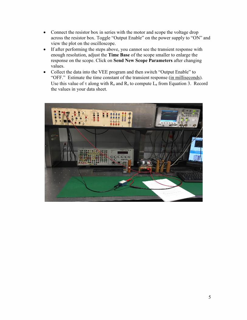
• Connect the resistor box in series with the motor and scope the voltage drop across the resistor box. Toggle “Output Enable” on the power supply to “ON” and view the plot on the oscilloscope.

• If after performing the steps above, you cannot see the transient response with enough resolution, adjust the Time Base of the scope smaller to enlarge the response on the scope. Click on Send New Scope Parameters after changing values.

• Collect the data into the VEE program and then switch “Output Enable” to “OFF.” Estimate the time constant of the transient response (in milliseconds). Use this value of τ along with Ra and Rs to compute La from Equation 3. Record the values in your data sheet.

6

3.7 Back – EMF Constant and Viscous Friction Coefficient The goal of this section will be to compute the back – EMF constant, Kb. To do so, the motor will be permitted to rotate and measurements will be taken when the system has reached its steady state. Consider Equation 1. Once steady state has been reached, Ia will be constant. Therefore, the derivative of the current will be zero. Substituting Equation 2 into Equation 1 yields Equation 4:

Equation 4

ωbaaa KRIE += The motor angular velocity, ω, can be found by measuring the tachometer voltage and using the gain found in Lab 1. Since Kb = KT (in the SI system, as you proved in the prelab), finding Kb will give KT. At steady state conditions, combining Equation 5 and Equation 6 yields Equation 7, which allows us to compute the viscous Friction Coefficient (B).

Equation 5: Torque – current Equation

)(tiKT aTm =

Equation 6: Mechanical equation 2

2

( ) ( )m

d t d tT J Bdt dtθ θ

= + ( )d tdtθ ω=

Equation 7

ωBIK aT = Follow the directions below:

• Remove the rotor–locking attachment and the resistor box. Connect the power supply directly to the motor.

• Use the DMM (Digital Multimeter) to measure the tachometer voltage. The orange terminal of the tachometer is the positive lead and the gray terminal is the negative lead.

• Open the Agilent VEE file: “n:/labs/se320/exp3/kb-n-b.vxe” • From the computer “Reset” the power supply and then switch “Output Enable” to

off. Set the current to 2 amps and the voltage to 7.5V. • Switch “Output Enable” to on and allow the system to reach its steady state (a

couple of seconds will be more than sufficient). Measure the applied voltage (Ea), the steady–state current (Ia) drawn by the motor, and the voltage generated by the tachometer.

• Turn off the power supply using “Output Enable”. • Compute motor angular velocity, ω, and parameters Kb, KT, and B. Record these

values. • Repeat the experiment with 10V applied to the motor.

7

3.8 Rotor Moment of Inertia The motor’s moment of inertia, J, and the friction coefficient, B, establish the angular velocity decay rate once current to the motor has been cut. Equation 6 links J and B to the time constant of the velocity decay, since T m = 0 when the current is zero. You should have determined B in previous section. With B known, we can find J (τm = J/B). A thumb switch is used to cut the current instantaneously. If you are not clear where τm = J/B came from, ask your TA for further explanation (Hint: Take Laplace transform of Equation 6, set to zero, and rearrange to resemble a first order transfer function for ω(s)).

• Connect the Thumb-Switch Box in series with the motor. Depressing the thumb switch will disconnect the power supply from the motor.

• Scope the tachometer’s output voltage using channel 1 on the oscilloscope. • Open the file “n:/labs/se320/exp3/j.vxe.” Reset the power supply, toggle

“Output Enable” to “OFF,” and set the current to 2 amps and voltage to 15V. Set the scope’s Time Base to 200ms.

• Toggle the power supply’s output to “ON” and wait a second for the motor to reach steady state. Disconnect the motor from the power supply by pressing thumb switch, and watch the voltage display on the scope. Quickly press the “Stop” button on the scope to store the waveform, which should be an exponential decay.

• Estimate the time-constant τm. Using the values of B and τm, calculate J. • Make sure that all values are recorded in your data sheet.

8

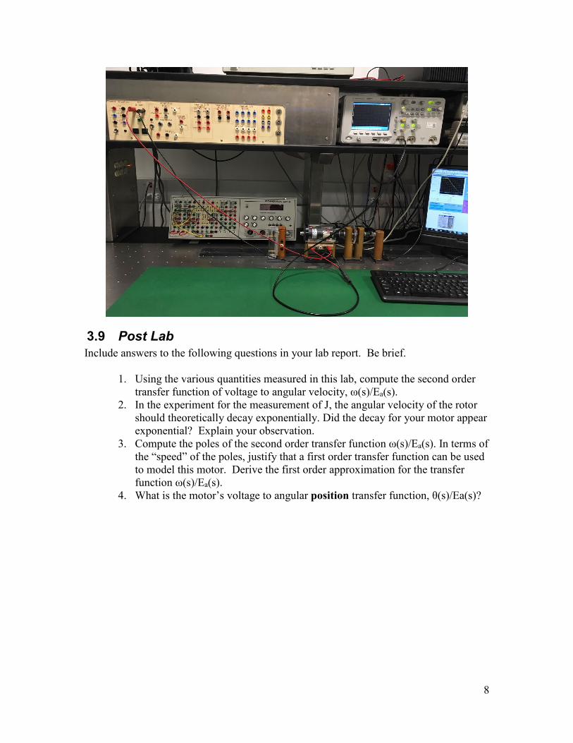
3.9 Post Lab Include answers to the following questions in your lab report. Be brief.

1. Using the various quantities measured in this lab, compute the second order transfer function of voltage to angular velocity, ω(s)/Ea(s).

2. In the experiment for the measurement of J, the angular velocity of the rotor should theoretically decay exponentially. Did the decay for your motor appear exponential? Explain your observation.

3. Compute the poles of the second order transfer function ω(s)/Ea(s). In terms of the “speed” of the poles, justify that a first order transfer function can be used to model this motor. Derive the first order approximation for the transfer function ω(s)/Ea(s).

4. What is the motor’s voltage to angular position transfer function, θ(s)/Ea(s)?

9

3.10 Data Sheet

Armature Resistance Current Voltage Ra

Average

Armature Inductance Resistor Box resistance (Rs) Time Constant (τ) Armature Inductance (La)

Back – EMF Constant and Viscous Friction Coefficient Ea Ia ω Vtach Kb (=Kt) B

7.5V 10V

Rotor Moment of Inertia Time Constant (τ) Moment of Inertia (J)