E x p e r i m e n t – 5

DC Motor Speed Control

5.1 Introduction

In experiment-3 and 4, the speed of the DC-motor was controlled by using an open-loop voltage

control. The purpose of this experiment is to design and implement a close-loop speed control of a

DC-motor drive. We shall use the same DC-motor for which the parameters were calculated in the

previous experiment. At first, the controllers will be designed and tested on a simulation model of

the DC-motor. Once the parameters are tuned, the model of the DC-motor will be replaced with the

real motor. The tuned controllers will be implemented in real-time on DS1104 to perform the

close-loop speed control of the DC-motor.

5.2 Simulink Model of the DC-motor

The model for a DC-motor in frequency domain is derived in Chapter 8 [1].

)s(k)s(EsLR

)s(E)s(V)s(I mEa

aa

aaa

(1)

ETaTemeq

Lemm kk)s(Ik)s(T

sJ

)s(T)s(T)s(

(2)

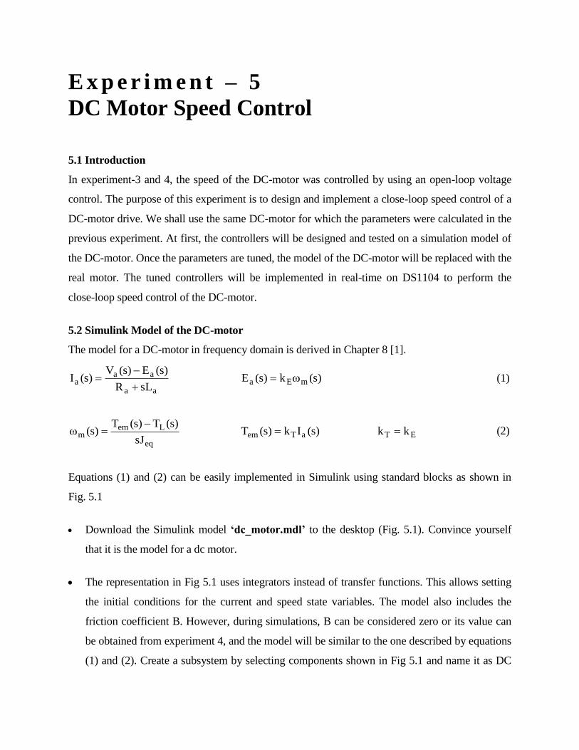
Equations (1) and (2) can be easily implemented in Simulink using standard blocks as shown in

Fig. 5.1

Download the Simulink model ‘dc_motor.mdl’ to the desktop (Fig. 5.1). Convince yourself

that it is the model for a dc motor.

The representation in Fig 5.1 uses integrators instead of transfer functions. This allows setting

the initial conditions for the current and speed state variables. The model also includes the

friction coefficient B. However, during simulations, B can be considered zero or its value can

be obtained from experiment 4, and the model will be similar to the one described by equations

(1) and (2). Create a subsystem by selecting components shown in Fig 5.1 and name it as DC

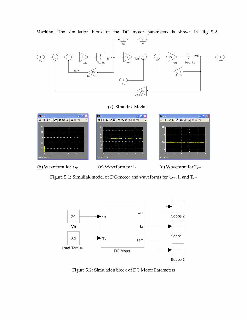
Machine. The simulation block of the DC motor parameters is shown in Fig 5.2.

1/LVa

+-

1 +-

+-

+-

2

2

3

11/L

Vtg int

IaKe

ke

Tem

TemIa

I/J

Jeq Mech int

wm

wm

0

BRa

RaIaRa

TL

Ke

Gain 5

1

s

1

s

(a) Simulink Model

(b) Waveform for m (c) Waveform for Ia (d) Waveform for Tem

Figure 5.1: Simulink model of DC-motor and waveforms for m, Ia and Tem

Figure 5.2: Simulation block of DC Motor Parameters

Va

20

Scope 3

Scope 2

Scope 1

Load Torque

0.1

DC Motor

Va

TL

wm

Ia

Tem

Now enter the values of DC-motor parameters, which were evaluated in experiment – 3 and 4

in file ‘dc_motor_parameters.m’. Ia_initial, wm_initial are the initial values for the

integrator. To observe the zero initial condition response, set these values to zero. Run this file.

Make sure your units are all consistent.

Run the simulation (with default configuration parameters) for the following two cases.

Compare the observed values with calculated values. Save the plots and include them in your

report.

a) Va = 20V, Load_Torque = 0.3 Nm

b) Va = 20V, Load_Torque = 0 Nm

5.3 Controller Design

Once the DC-motor model is built, the controllers can be added and tuned. Start with the current

loop for which a PI controller is required.

Download the file ‘components.mdl’. All the necessary blocks can be copied from here. For

the more adventurous, follow the instructions as specified in points a, b, and c to build it!

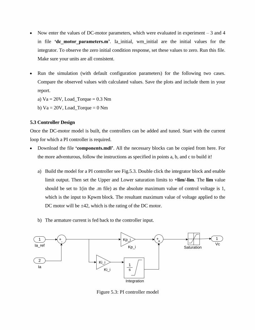
a) Build the model for a PI controller see Fig.5.3. Double click the integrator block and enable

limit output. Then set the Upper and Lower saturation limits to +lim/-lim. The lim value

should be set to 1(in the .m file) as the absolute maximum value of control voltage is 1,

which is the input to Kpwm block. The resultant maximum value of voltage applied to the

DC motor will be ±42, which is the rating of the DC motor.

b) The armature current is fed back to the controller input.

Ia_ref

+-

1 ++

2

1

SaturationVc

Integration

Kp_i

Kp_i

Ki_i

Ki_iIa

1

s

Figure 5.3: PI controller model

c) The Saturation block sets the maximum and minimum limits for the control voltage (in our

case ±1).

Design current controller for a bandwidth of 100 Hz (628.3 rad/sec) (phase margin 90 deg).

The parameters of the PI controller (namely Kp_i and Ki_i) are computed using the motor

parameters, which were evaluated in the earlier experiment. This procedure is described in

section 8-7-1 [1] (Explained at the End after the Report because we don’t have the book).

Create the file for a current controlled DC motor as shown in Fig 5.4(a).

Running the Simulink model for the current controller with reference current as 2A, results

similar to the Fig.5.4 (b) and Fig. 5.4(c) will be obtained.

Set the value of Kp_i and Ki_i in Matlab prompt (or in the m file ‘dc_motor_parameters’).

Also set the values of lim = 1, Kpwm = 42, Ia_ref=1. Run the m-file before running the

simulation, which will load the values of all the variables. Run this simulation for a

reference current of 1 A (for 0.005 sec, variable step , time step 1e-4). Save the plots for the

report.

Once the response in current is considered optimal (low overshoot, fast rise-time, zero steady

state error), the speed controller can be designed. For designing the speed controller you can

assume B=0 but while building the Simulink block, include B.

A similar PI controller for the speed loop (‘PI_Speed’) will be added to the Simulink model.

Design the speed controller for a bandwidth of 10Hz (62.83 rad/sec) (Phase margin 60 deg).

Follow the procedure described in 8-7-2 [1] to design the speed control loop, using the motor

parameters determined in earlier experiment. (Explained at the End after the Report

because we don’t have the book).

0

Ia_ref

Ia_ref

Ia_ref

Ia

Vc KpwmV_motor

Va

TL

wm

Ia

Tem

wm

TerminatorDC Motor

Load

Torque

PI_Current Gain

Ia, Ia_ref

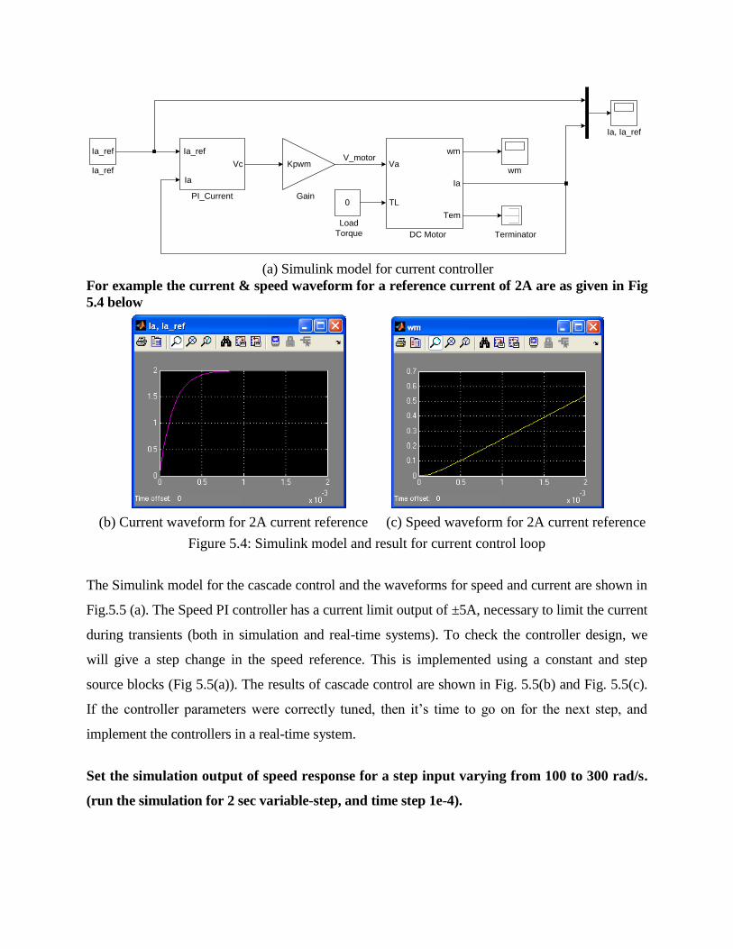
(a) Simulink model for current controller

For example the current & speed waveform for a reference current of 2A are as given in Fig

5.4 below

(b) Current waveform for 2A current reference (c) Speed waveform for 2A current reference

Figure 5.4: Simulink model and result for current control loop

The Simulink model for the cascade control and the waveforms for speed and current are shown in

Fig.5.5 (a). The Speed PI controller has a current limit output of ±5A, necessary to limit the current

during transients (both in simulation and real-time systems). To check the controller design, we

will give a step change in the speed reference. This is implemented using a constant and step

source blocks (Fig 5.5(a)). The results of cascade control are shown in Fig. 5.5(b) and Fig. 5.5(c).

If the controller parameters were correctly tuned, then it’s time to go on for the next step, and

implement the controllers in a real-time system.

Set the simulation output of speed response for a step input varying from 100 to 300 rad/s.

(run the simulation for 2 sec variable-step, and time step 1e-4).

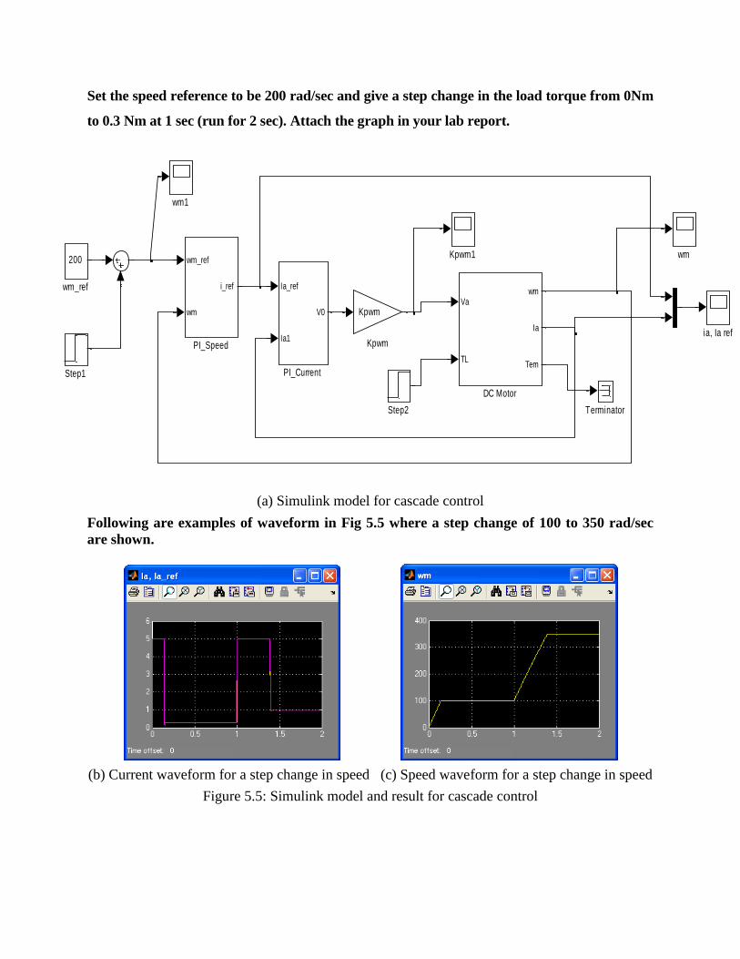
Set the speed reference to be 200 rad/sec and give a step change in the load torque from 0Nm

to 0.3 Nm at 1 sec (run for 2 sec). Attach the graph in your lab report.

(a) Simulink model for cascade control

Following are examples of waveform in Fig 5.5 where a step change of 100 to 350 rad/sec

are shown.

(b) Current waveform for a step change in speed (c) Speed waveform for a step change in speed

Figure 5.5: Simulink model and result for cascade control

200

wm_ref

wm1

wm

ia, Ia ref

TerminatorStep2

Step1

wm_ref

wm

i_ref

PI_Speed

Ia_ref

Ia1

V0

PI_Current

Kpwm1

Kpwm

Kpwm

Va

TL

wm

Ia

Tem

DC Motor

5.4 Real-time implementation of feedback control

For dSPACE implementation, the dc-motor model will be replaced with the real motor and power

converter with 42V dc supply will replace Kpwm block. The control voltage to duty cycle

conversion was already discussed and implemented in experiment – 2.

All the necessary components to make the model in Fig 5.7 are provided in the file

‘components.mdl’. If you would like to build it the instructions as in a to f are given below:

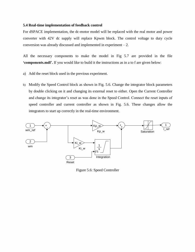
a) Add the reset block used in the previous experiment.

b) Modify the Speed Control block as shown in Fig. 5.6. Change the integrator block parameters

by double clicking on it and changing its external reset to either. Open the Current Controller

and change its integrator’s reset as was done in the Speed Control. Connect the reset inputs of

speed controller and current controller as shown in Fig. 5.6. These changes allow the

integrators to start up correctly in the real-time environment.

wm_ref

+-

1 ++

2

1

SaturationI_ref

Integration3

Kp_w

Kp_w

Ki_w

Ki_wwm

Reset

1

s

Figure 5.6: Speed Controller

1 0

0

-1

Gain1

constant

Gain2

1/2

dC

PWM Control

++

Duty cycle b

Duty cycle a

Duty cycle c

PWM Stop

DS1104SL_DSP_PWM3

1 booleanSLAVE BIT

OUT

DS1104 SL_DSP_BIT_OUT_C10Data type Conversion 2Reset

ADC 20

motor_currentDS1104 ADC_C5

Ia_ref

Ia 1 Vc

wm_ref

wm i_ref

reset

reset

DS1104 ENC_POS_CI

DS1104 ENC_SETUP

Encoder

Master Setup

Enc position

Enc delta position

Gain 5

2*pi / (Ts*1000) Wm_dist Wm

Avg Block

motor_speed

1

PI_Speed_reset

PI_Current_reset

Wref_4quad

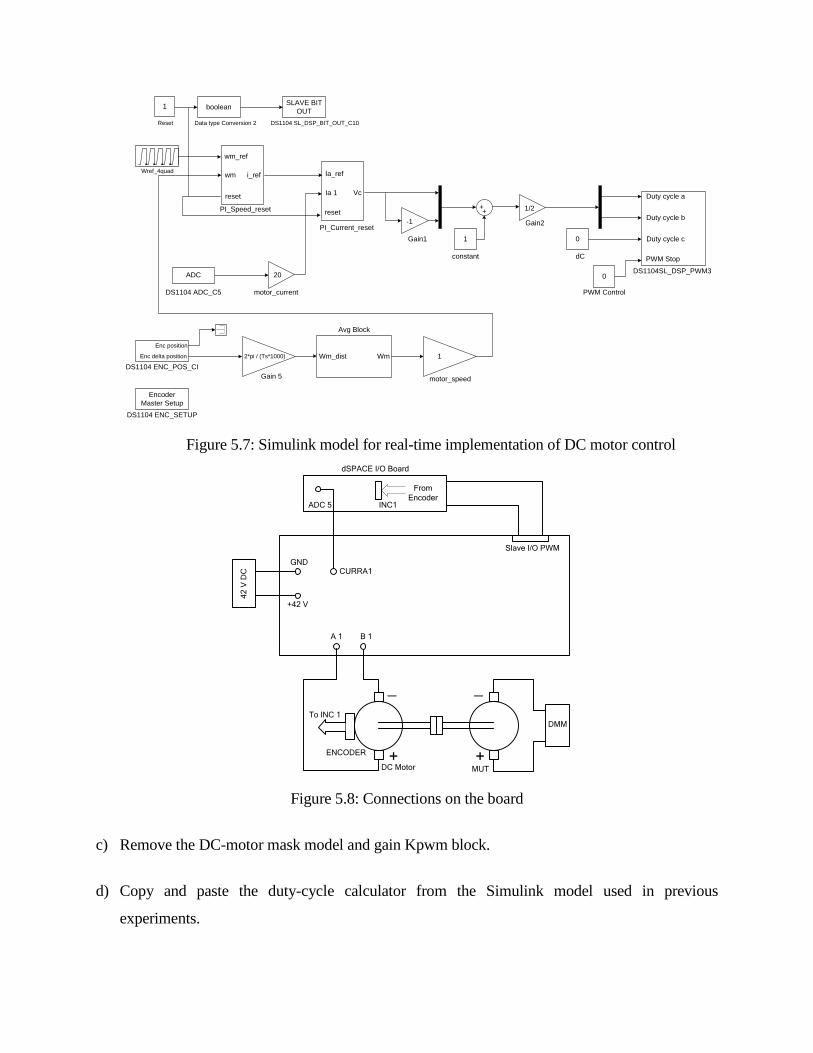
Figure 5.7: Simulink model for real-time implementation of DC motor control

ADC 5 INC1

From

Encoder

dSPACE I/O Board

CURRA1GND

+42 V

42

V D

C

B 1A 1

ENCODER

To INC 1

+

_

+

_

MUT

DMM

Slave I/O PWM

DC Motor

Figure 5.8: Connections on the board

c) Remove the DC-motor mask model and gain Kpwm block.

d) Copy and paste the duty-cycle calculator from the Simulink model used in previous

experiments.

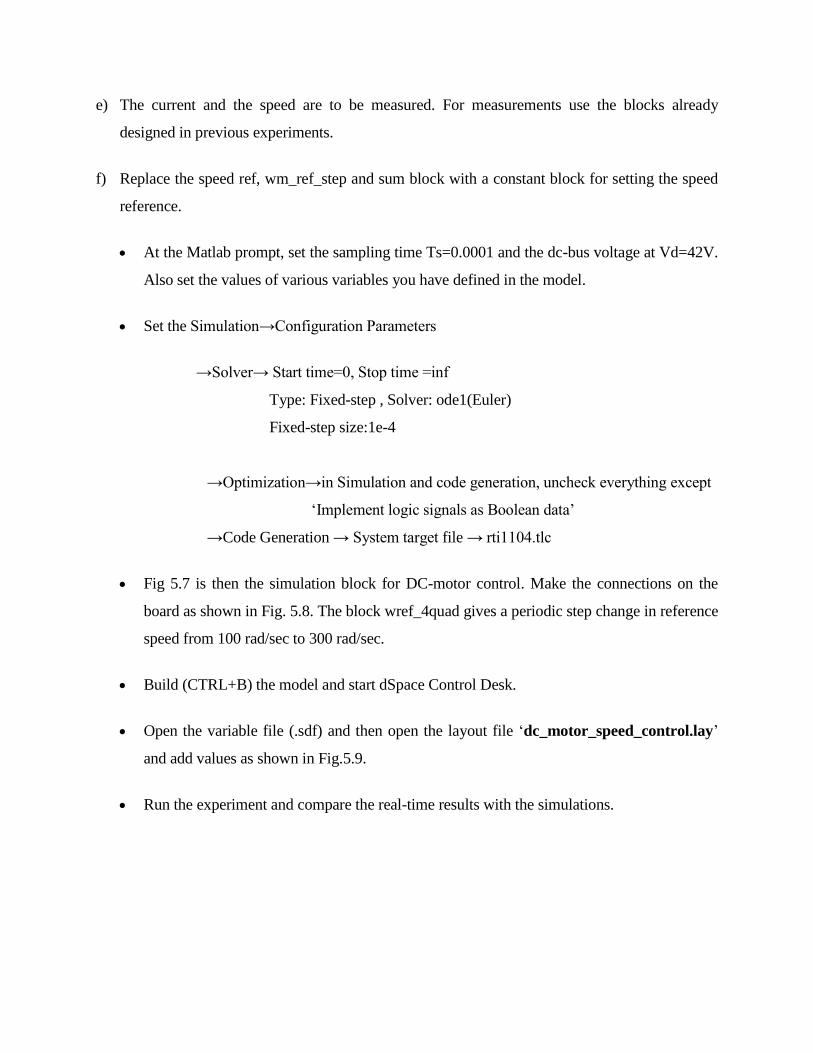
e) The current and the speed are to be measured. For measurements use the blocks already

designed in previous experiments.

f) Replace the speed ref, wm_ref_step and sum block with a constant block for setting the speed

reference.

At the Matlab prompt, set the sampling time Ts=0.0001 and the dc-bus voltage at Vd=42V.

Also set the values of various variables you have defined in the model.

Set the Simulation→Configuration Parameters

→Solver→ Start time=0, Stop time =inf

Type: Fixed-step , Solver: ode1(Euler)

Fixed-step size:1e-4

→Optimization→in Simulation and code generation, uncheck everything except

‘Implement logic signals as Boolean data’

→Code Generation → System target file → rti1104.tlc

Fig 5.7 is then the simulation block for DC-motor control. Make the connections on the

board as shown in Fig. 5.8. The block wref_4quad gives a periodic step change in reference

speed from 100 rad/sec to 300 rad/sec.

Build (CTRL+B) the model and start dSpace Control Desk.

Open the variable file (.sdf) and then open the layout file ‘dc_motor_speed_control.lay’

and add values as shown in Fig.5.9.

Run the experiment and compare the real-time results with the simulations.

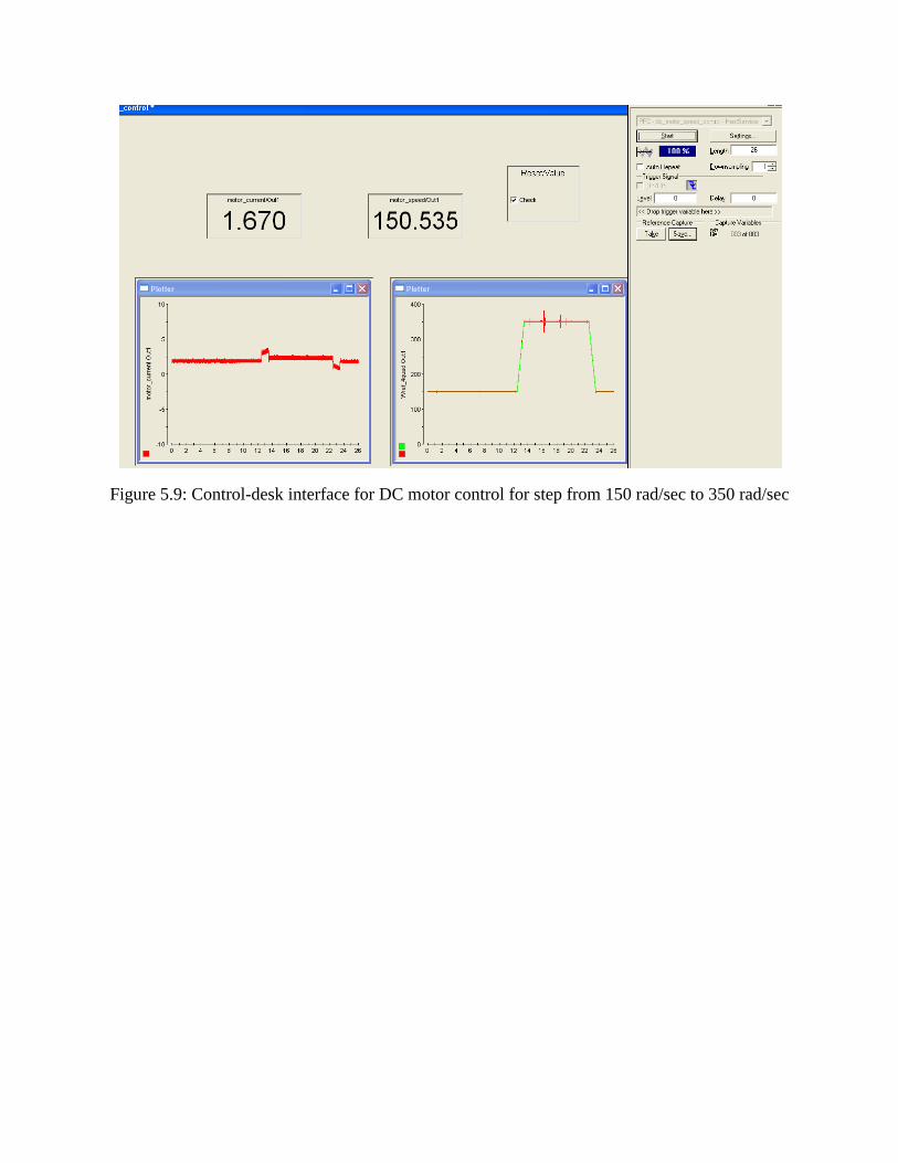
Figure 5.9: Control-desk interface for DC motor control for step from 150 rad/sec to 350 rad/sec

Lab Report (10points)

1. Section 5.2: Run the simulation (with default configuration parameters for 10 sec) for the

following two cases. Check the observed values with calculated values (show your

calculations). Save the plots and include them in your report. (2points)

a) Va=20V, Load_Torque = 0.3 Nm

b) Va=20V, Load_Torque = 0 Nm

2. Section 5.3:

a) Report your calculations for current and speed controller. Note: Design current controller

for a bandwidth of 100 Hz (phase margin 90 deg) and speed controller for a bandwidth of

10Hz (Phase margin 60 deg). For designing the speed controller you can assume B=0 but

while building the Simulink block, include B. (2 points)

b) Attach simulation output of current response for a step input of 1A. (1 point)

c) Attach simulation output of speed response for a step input of 200 rad/s from a constant

value of 100 rad/s ( 1 point)

d) All the responses required for questions 2b) and 2c) are based on step change in reference

signals. These are required more for design purposes. In practical applications, it is more

important to know how the system responds to disturbances in load torque. In the

simulation, give a step load torque of 0.3 N-m while maintaining a constant speed of 200

rad/s. Observe the response in current and speed and attach the plots. (1 points)

3. Section 5.4: Attach the speed and current response for a step change in speed reference as

observed through control-desk for a step change from 100 rad/sec to 300 rad/sec. (3 points)

References

[1] “ELECTRIC DRIVES an integrative approach” by Ned Mohan, 2000, MNPERE.

Important Calculations :

Some Calculation needed in Expierment 5, because we don’t have the book Ref [1]

This is the summary ( procedure) of the sections 8-7-1 and 8-7-2

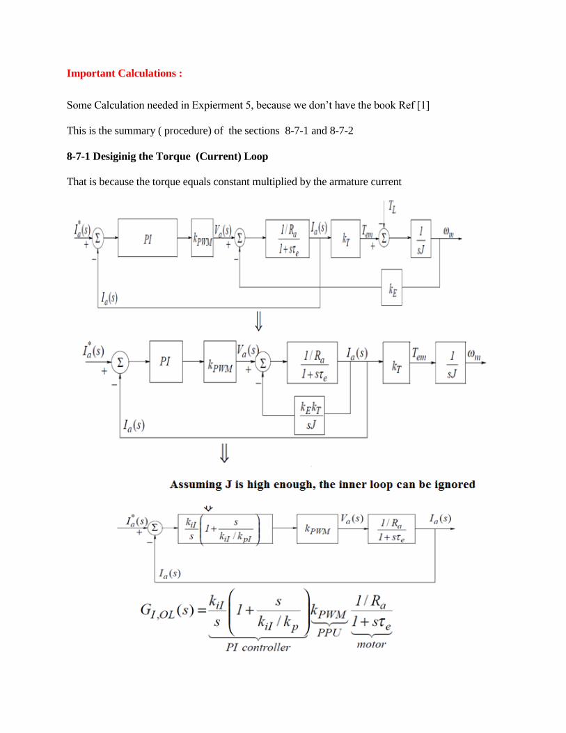
8-7-1 Desiginig the Torque (Current) Loop

That is because the torque equals constant multiplied by the armature current

Ki_i and Kp_i is determined as follows :

Where

electric Time Constant

From (1)

Where and is the crossover frequency (Band Width frequency)

The procedure is to find Ki_i from equation (4) and then substitute it back in equation (1) to find

Kp_i

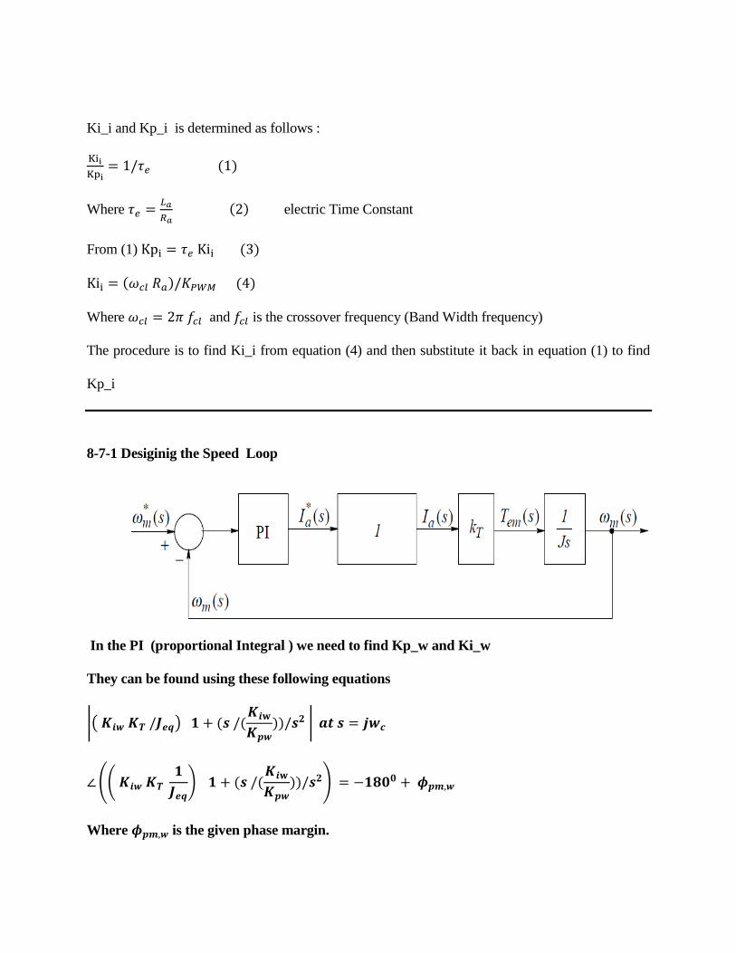
8-7-1 Desiginig the Speed Loop

In the PI (proportional Integral ) we need to find Kp_w and Ki_w

They can be found using these following equations

|( )

|

((

)

)

Where is the given phase margin.