1

Experiment #9: RC and LR Circuits—Time Constants Purpose: To study the charging and discharging of capacitors in RC circuits and the growth and decay of current in LR circuits. Part 1—Charging RC Circuits Discussion:

A capacitor stores separated charges for later use. The capacitance C of a capacitor is defined as the absolute value of the ratio of the charge Q on either plate to the potential difference VC between the plates, C ! Q /V

C (1)

with units of C/V ≡ F (farads). A farad is a very large unit; typical capacitors used in electronic circuits have values in the range of µF, nF, or even pF.

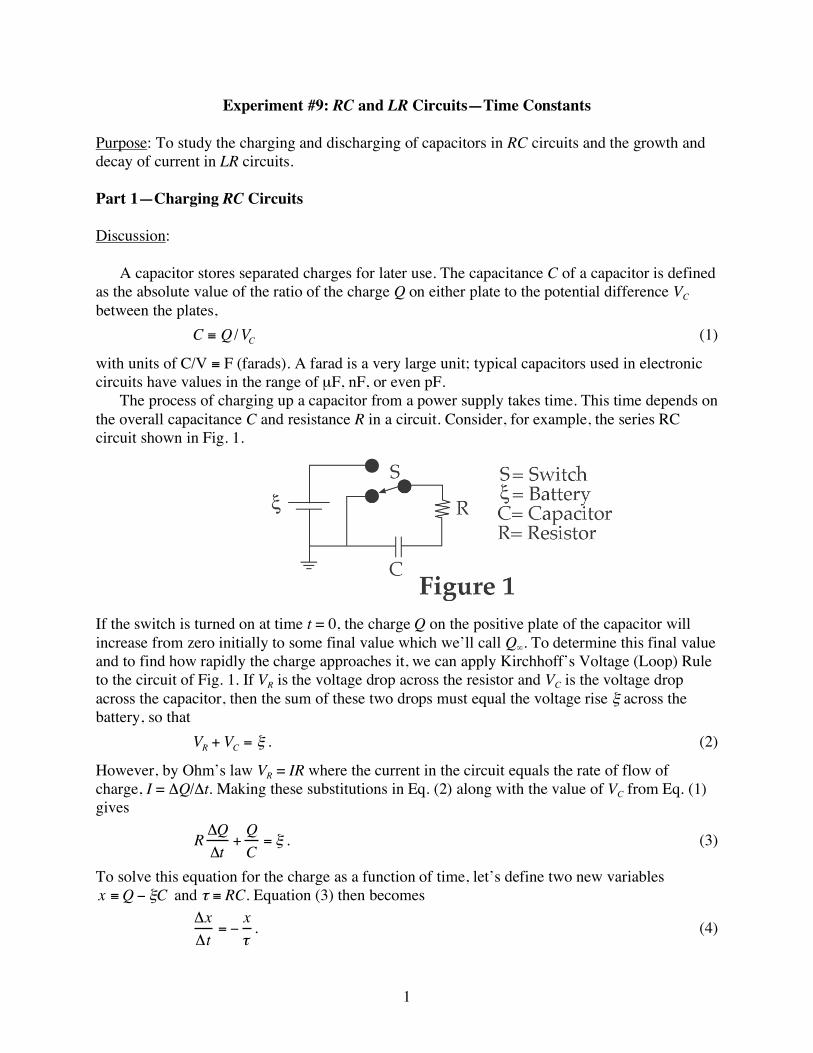
The process of charging up a capacitor from a power supply takes time. This time depends on the overall capacitance C and resistance R in a circuit. Consider, for example, the series RC circuit shown in Fig. 1.

If the switch is turned on at time t = 0, the charge Q on the positive plate of the capacitor will increase from zero initially to some final value which we’ll call Q∞. To determine this final value and to find how rapidly the charge approaches it, we can apply Kirchhoff’s Voltage (Loop) Rule to the circuit of Fig. 1. If VR is the voltage drop across the resistor and VC is the voltage drop across the capacitor, then the sum of these two drops must equal the voltage rise ξ across the battery, so that V

R+ V

C= ! . (2)

However, by Ohm’s law VR = IR where the current in the circuit equals the rate of flow of charge, I = ΔQ/Δt. Making these substitutions in Eq. (2) along with the value of VC from Eq. (1) gives

R!Q

!t+Q

C= " . (3)

To solve this equation for the charge as a function of time, let’s define two new variables x !Q " #C and τ ≡ RC. Equation (3) then becomes

!x

!t= "

x

#. (4)

2

Supplemental Question 1: Show that Eq. (4) is equivalent to Eq. (3). Hint: !("C) = 0 since both ξ and C are constants.

Thus if we were to make a graph of x versus t, we would find that the slope Δx/Δt of this function is always proportional to the value x of the function. This is the defining property of the exponential function, and hence the solution of Eq. (4) is x = x

0e! t / " (5)

where you can see that x0 is the value of x at t = 0. Since Q = 0 at that time, x0= !"C .

Supplemental Question 2 (University Physics students only): To be more exact, we should be taking the limit as !t" 0 in Eqs. (3) and (4). Thus, the left-hand side of Eq. (4) actually becomes the derivative dx/dt. Now show that Eq. (5) is a solution of this corrected version of Eq. (4).

Finally, we replace x with our original circuit variables in Eq. (5) and rearrange to obtain Q =Q!(1 " e

"t / #) (6)

where Q! " #C is the final charge on the positive plate of the capacitor. This value of Q∞ makes intuitive sense: after the circuit has settled down and current has stopped flowing, there is no voltage drop across the resistor (because of Ohm’s law) and hence the entire battery voltage ξ appears across the capacitor, so that Q! = "C from Eq. (1). Note in Eq. (6) that τ ≡ RC has SI units of seconds (if R is in Ω and C is in F) and is called the time constant of the circuit.

A plot of Eq. (6) as a function of time is shown in Fig. 2 above, using the values Q∞ = 2 nC and τ = 0.1 s.

Fig. 2. Charging a capacitor in an RC circuit.

0

0.5

1

1.5

2

0 0.2 0.4 0.6

t (s)

3

Supplemental Question 3: Suppose a 1.5-V battery, a 20-nF capacitor, and a 150-kΩ resistor are connected in series. Compute the time constant τ in ms and final capacitor charge Q∞ in nC.

You will notice in Fig. 2 that it took half a second for the charge to approximately reach its final value. More exactly however, Eq. (6) tells us that the charge Q only reaches the final value Q∞ asymptotically, that is in the limit as t! " . Since this is not very informative, it is conventional to use the time constant τ as a measure of how quickly the capacitor charges up. Notice from Eq. (6) that the capacitor attains 63.2% of its final charge in this time, because

t = ! "Q

Q#

=1 $ e$1= 0.632 . (7)

Supplemental Question 4: What percentage of the final charge does the capacitor attain after 3 time constants? After 5 time constants? You should find results consistent with Fig. 2, thus explaining why the charge can be considered to have reached its final value after about 0.5 s. Thus, for the circuit parameters given in Supplemental Question 3, after how long can the capacitor be considered to have reached full charge?

We can use Eq. (6) to find the voltages and current in the circuit. Substituting Eq. (6) into (1) implies that V

C= !(1" e

"t / #) , (8)

where use was made of the fact that Q! " #C . Equation (8) tells us that a graph of VC would have the same shape as Fig. 2: the capacitor’s charge and voltage rise up together to their respective final values of Q∞ and ξ. On the other hand, since V

R= ! " V

C (from Kirchhoff’s Voltage Rule),

Eq. (8) implies that V

R= !e

"t / # , (9) or equivalently, since I = VR/R (from Ohm’s law), I = I

0e!t / " (10)

where I0! " / R is the initial current which flows in the circuit in the instant after switch S is

turned on. Equations (9) and (10) tell us that the resistor’s voltage and current start out with their maximum values of ξ and I0, respectively, but fade away together to zero as t! " . Graphs of these two quantities thus have the same shape as Fig. 5 below.

The limits of our results are easy to interpret. Putting t = 0 into Eqs. (6) and (8) to (10) gives Q = VC = 0 which makes sense because initially the capacitor is uncharged and there is no potential difference across it, while VR = ξ and I = ξ/R because all of the battery voltage must thus appear across the resistor. On the other hand, putting t! " gives VR = I = 0 because the circuit has finally settled down and no further current flows (owing to the presence of the capacitor which makes it an open circuit), while VC = ξ and Q = !C since all of the battery voltage must thus appear across the fully charged capacitor.

4

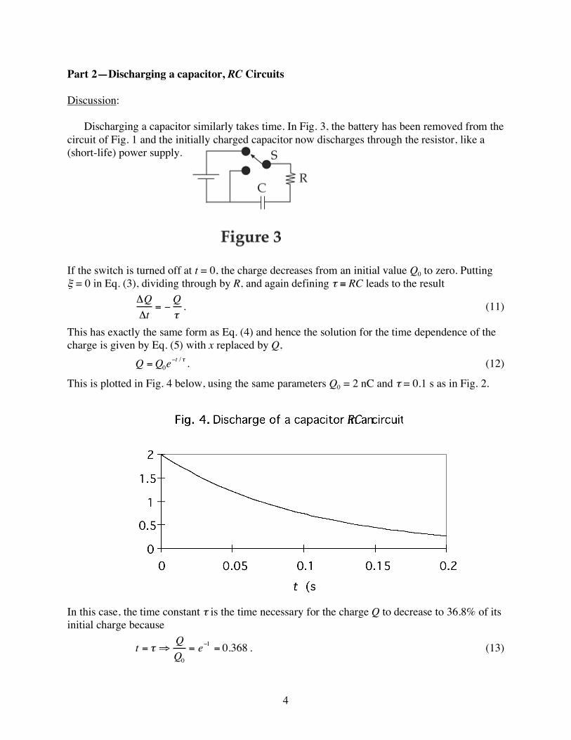
Part 2—Discharging a capacitor, RC Circuits Discussion:

Discharging a capacitor similarly takes time. In Fig. 3, the battery has been removed from the circuit of Fig. 1 and the initially charged capacitor now discharges through the resistor, like a (short-life) power supply.

If the switch is turned off at t = 0, the charge decreases from an initial value Q0 to zero. Putting ξ = 0 in Eq. (3), dividing through by R, and again defining τ ≡ RC leads to the result

!Q

!t= "

Q

#. (11)

This has exactly the same form as Eq. (4) and hence the solution for the time dependence of the charge is given by Eq. (5) with x replaced by Q, Q =Q

0e!t / " . (12)

This is plotted in Fig. 4 below, using the same parameters Q0 = 2 nC and τ = 0.1 s as in Fig. 2.

In this case, the time constant τ is the time necessary for the charge Q to decrease to 36.8% of its initial charge because

t = ! "Q

Q0

= e#1= 0.368 . (13)

5

We can use Eq. (12) to again find the voltages and current in the circuit, like we did in Part 1. Substituting Eq. (12) into (1) implies that V

C= !e

"t / # , (14)

assuming that the capacitor was initially fully charged using the circuit of Fig. 1, so that Q0=Q! " #C . Equation (14) tells us that a graph of VC would have the same shape as Fig. 4: the

capacitor’s charge and voltage decay away together to zero. On the other hand, since VR+ V

C= 0

(from Kirchhoff’s Voltage Rule), Eq. (14) implies that V

R= !"e

!t / # , (15) or equivalently, since I = VR/R (from Ohm’s law), I = ! I

0e!t / " (16)

where I0! " / R is the initial current which flows in the circuit in the instant after switch S is

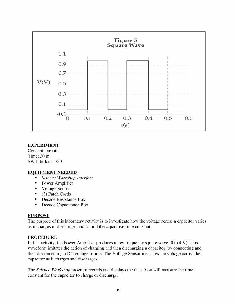
turned on. Equations (15) and (16) tell us that the absolute value of the resistor’s voltage and current start out at maximums of ξ and I0, respectively, but fade away together to zero as t! " . The negative signs indicate that the current is counter-clockwise (rather than clockwise as in Fig. 1) and that in going around the circuit in this counter-clockwise direction, the potential rises in going across the capacitor (because it acts like a battery) but drops in going across the resistor. Graphs of these two quantities thus have the same shape as Fig. 4 above, except that they must be flipped over by mirror-reflecting them across the horizontal axis. Supplemental Question 5 (University Physics students only): By definition, I ! dQ / dt . Substitute Eqs. (12) and (16) into this and verify that an equality results, using the definitions given above for τ, Q0, and I0. Discussion on experimental technique: The role of a function generator or signal generator The circuits, which we will study and also those in general use have time constants which are smaller than 0.1 s, so it is impractical to think of building a circuit like Figure 1 or Figure 3 with a manual on/off switch. What we would like to have is a device, which acts like a battery, but whose output voltage can be suddenly cut off to zero, or put on to say 5 V, in a preprogrammed fashion. This is accomplished by a signal generator. The “Power Amplifier” (PASCO CI-6552A and the PASCO 750 Interface that drives it) on your table does the job of a signal generator. The “SIGNAL OUTPUT” on the front panel can be set to output a voltage, which is called a “Square Wave” and looks like the graph shown in Figure 5 below. In this case, the output voltage swings from 0 V to 1 V and back again every 0.1 s. If we put a power supply like that in place of the battery in our circuit of Figure 1, then during the time when the output is 1 V, effectively there is a battery of 1 V in the circuit, and the capacitor gets charged, and during the time when the output is 0 V, there is no battery in the circuit, and the capacitor gets discharged. Function generators have capabilities of changing the voltage swing, the time period, and even the form of the wave to produce sine waves and triangular waves.

6

EXPERIMENT: Concept: circuits Time: 30 m SW Interface: 750 EQUIPMENT NEEDED

• Science Workshop Interface • Power Amplifier • Voltage Sensor • (3) Patch Cords • Decade Resistance Box • Decade Capacitance Box

PURPOSE The purpose of this laboratory activity is to investigate how the voltage across a capacitor varies as it charges or discharges and to find the capacitive time constant. PROCEDURE In this activity, the Power Amplifier produces a low frequency square wave (0 to 4 V). This waveform imitates the action of charging and then discharging a capacitor, by connecting and then disconnecting a DC voltage source. The Voltage Sensor measures the voltage across the capacitor as it charges and discharges. The Science Workshop program records and displays the data. You will measure the time constant for the capacitor to charge or discharge.

7

PART I: Computer Setup

1. Connect the Science Workshop interface to the computer, turn on the interface, and turn on the computer.

2. Connect the Voltage Sensor to Analog Channel A. Connect the Power Amplifier to

Analog Channel B. Plug the power cord into the back of the Power Amplifier and connect the power cord to an appropriate electrical outlet.

3. Open the Science Workshop document titled as shown:

RC1.SWS This file is in the phylabii folder on the desktop of your computer.

• The document opens with a Graph display of Voltage (V) versus Time (sec), and the Signal Generator window, which controls the Power Amplifier.

• Note: For quick reference, see Experiment Notes window. To bring a display to the top,

click on its window or select the name of the display from the list at the end of the Display menu. Change the Experiment Setup window by clicking on the Zoom box or the Restore button in the upper right hand corner of that window.

4. The Sampling Options…for this activity are: Periodic Samples = Fast at 1000 Hz and

Stop Condition = Time at 4.00 seconds.

5. The Signal Generator is already set to output 2.00 V, “positive only” square AC Waveform, at 1.00 Hz. It is set to Auto so the Signal Generator will start automatically when you click MON or REC and stop automatically when you click STOP or PAUSE.

Part II: Sensor Calibration and Equipment Setup

• You do not need to calibrate the Voltage Sensor or the Power Amplifier. You will use a resistance box and a capacitance box in your circuit. These are really boxes with knobs which allow you to vary the values of R and C in the circuit. Connect the circuit as shown in Figure 1, using the output of the Signal Generator in place of the battery. Use the H and L terminals on the resistance box and the red and black terminals on the capacitance box for connections. SHOW THE CIRCUIT TO YOUR INSTUCTOR BEFORE TURNING IT ON!!

1. Set the resistance box to 20 kΩ, and the capacitance to 0.5 µF.

2. Connect the Voltage Sensor banana plugs to the red and black terminals of the capacitor.

This will measure the voltage across the capacitor.

8

Part III: Data Recording

1. Turn on the power switch on the back of the Power Amplifier. 2. Click the REC button to start collecting data. The Signal Generator output will

automatically start when data recording begins.

3. Data recording will continue for four seconds and then stop automatically.

• Run #1 will appear in the Data list in the Experiment Setup window.

4. When the data recording is complete, turn off the switch on the back of the Power Amplifier.

ANALYZING DATA

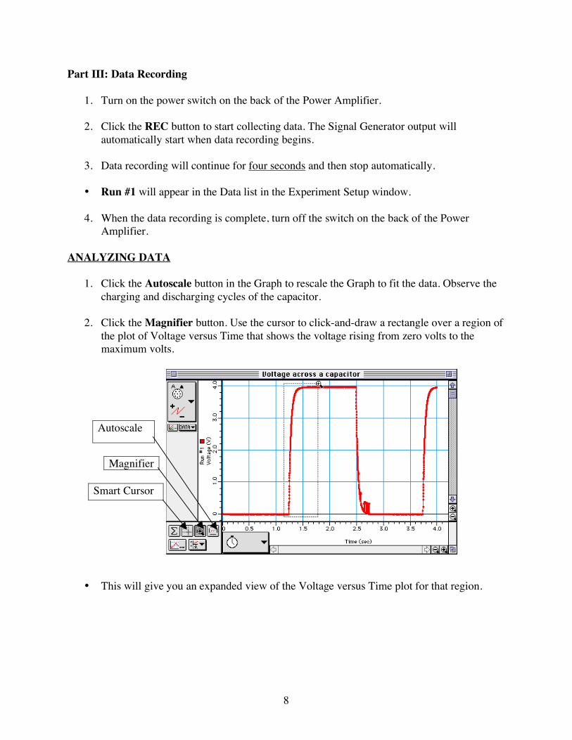
1. Click the Autoscale button in the Graph to rescale the Graph to fit the data. Observe the charging and discharging cycles of the capacitor.

2. Click the Magnifier button. Use the cursor to click-and-draw a rectangle over a region of

the plot of Voltage versus Time that shows the voltage rising from zero volts to the maximum volts.

Autoscale

Magnifier

Smart Cursor

• This will give you an expanded view of the Voltage versus Time plot for that region.

9

3. Click the Smart Cursor button. The cursor changes to a cross-hair when you move the cursor into the display area of the Graph.

• The Y-coordinate of the cursor/cross-hair is shown next to the vertical axis. • The X-coordinate of the cursor/cross-hair is shown next to the horizontal axis.

4. Move the cursor to the point on the plot where the voltage begins to rise. Record the time

that is shown in the area below the horizontal axis. 5. Move the Smart Cursor to the point where the voltage is approximately 0.632 x (max

input signal) volts. Record the new time that is shown in the area below the horizontal axis.

6. Find the difference between the two times and record it as τ.

ANALYZING THE DATA DATA Beginning time = __________s Time to 0.632 x Peak V = ___________s (Corrected for offset – Note 1 – Last Page) Time constant = __________s

1. Compare the measured time constant with the value of RC that you set in your circuit. 2. Use the percent difference method and compare the stated value (e.g., 0.01 s) to the

experimental value.

Further experimentation:

1. With the same data, you can see the discharge of the capacitor. Follow the same procedure, and determine τ again from the discharge data.

2. In the meanwhile, what is the resistor doing? What happens to the voltage across

the resistor, while the voltage across the capacitor is behaving like you just found out? You can answer this question, either by measurement, or by thinking about it. It is up to you. If you want to measure it, just disconnect the banana plugs of the voltage sensor from the capacitor, and connect them across the resistor, and make a run, and then compare it with the corresponding run where you measured the voltage across the capacitor.

3. Play with the setup. Change the values of R and C, run it again, and see what

happens. You don’t have to make measurements of τ each time, but if you like to, go ahead and record your measurement.

10

4. In the first setting, R = 10 kΩ, and C = 0.5 µF, so τ = 0.01 s. the signal generator was set for a frequency of 1 Hz. That means it was on for 0.5 s and off for 0.5 s. That is quite large compared to the time constant. What happens if you increase the frequency of the signal generator so that the “on time” is closer to the time constant? Check it and record your findings. What happens if the time constant is more than the on time?

Part 3—LR Circuits Discussion:

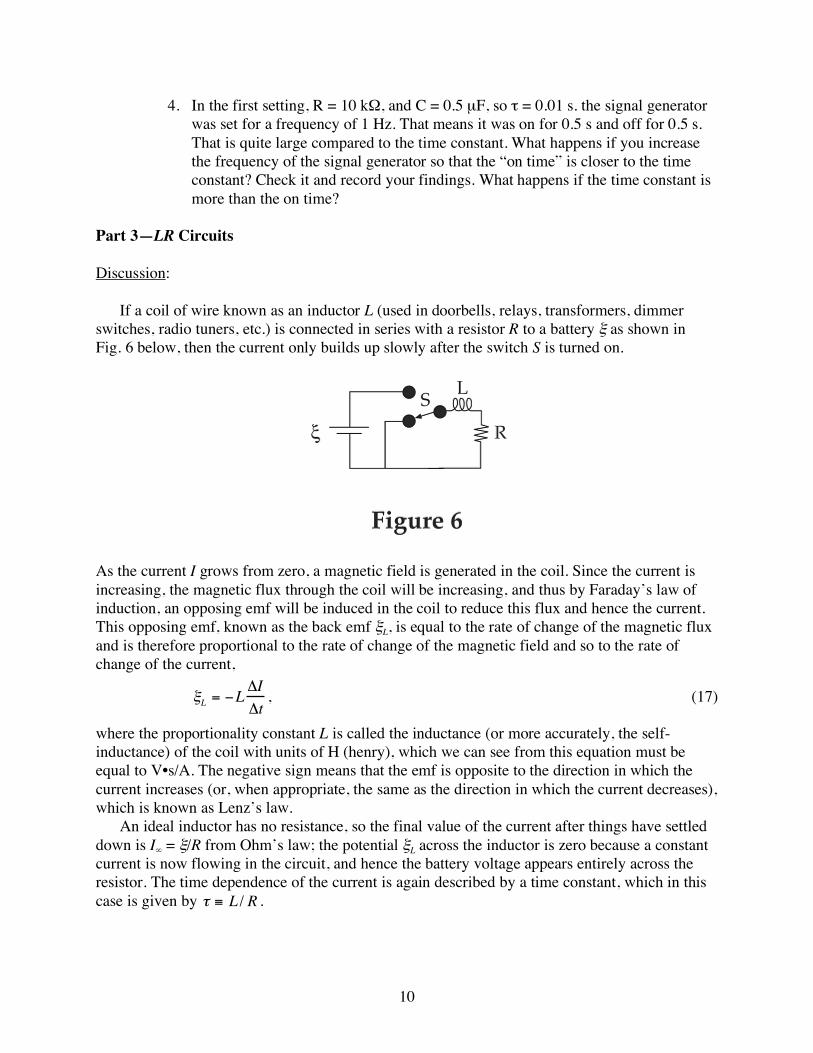
If a coil of wire known as an inductor L (used in doorbells, relays, transformers, dimmer switches, radio tuners, etc.) is connected in series with a resistor R to a battery ξ as shown in Fig. 6 below, then the current only builds up slowly after the switch S is turned on. As the current I grows from zero, a magnetic field is generated in the coil. Since the current is increasing, the magnetic flux through the coil will be increasing, and thus by Faraday’s law of induction, an opposing emf will be induced in the coil to reduce this flux and hence the current. This opposing emf, known as the back emf ξL, is equal to the rate of change of the magnetic flux and is therefore proportional to the rate of change of the magnetic field and so to the rate of change of the current,

!L= "L

#I

#t, (17)

where the proportionality constant L is called the inductance (or more accurately, the self-inductance) of the coil with units of H (henry), which we can see from this equation must be equal to V•s/A. The negative sign means that the emf is opposite to the direction in which the current increases (or, when appropriate, the same as the direction in which the current decreases), which is known as Lenz’s law.

An ideal inductor has no resistance, so the final value of the current after things have settled down is I∞ = ξ/R from Ohm’s law; the potential ξL across the inductor is zero because a constant current is now flowing in the circuit, and hence the battery voltage appears entirely across the resistor. The time dependence of the current is again described by a time constant, which in this case is given by ! " L / R .

11

Supplemental Question 6: Verify that L/R has units of seconds using the definition of henries above and the conversion of Ω to V and A from Ohm’s law.

The current is found to grow exponentially from zero according to the equation I = I!(1 " e

"t / #) , (18)

whose shape has already been plotted in Fig. 2. The current through an inductor builds up in an LR-series circuit, in exactly the same way that the charge on either capacitor plate builds up in an RC-series circuit. Supplemental Question 7: Derive Eq. (18) in exactly the same way that Eq. (6) was derived: (i) Kirchhoff’s Voltage Loop Rule implies that the sum of the emf’s of the battery and inductor equals the voltage drop across the resistor, ! +!

L= V

R. Substitute Eq. (17) for ξL and Ohm’s law

for VR, define ! " L / R and x ! I " # / R , and rearrange to obtain Eq. (4). A hint similar to that of Supplemental Question 1 applies here. (ii) The solution of Eq. (4) is again Eq. (5). Now replace x and x0 with the appropriate circuit variables, noting that the current is zero initially because the back emf cancels it out. Then rearrange to obtain Eq. (18).

In a loose sense, we can say that the inductor stores current, in the same way that a capacitor stores charge. (More exactly, we can say that both store electromagnetic energy.) If we remove the battery from the circuit in Fig. 6, the energized inductor will act like a short-life current supply, just as the energized capacitor in Fig. 4 acted like a short-life voltage supply. In both cases, the resulting current is given by Eq. (16): it is counter-clockwise and gradually decays away to zero. Experimental Setup: Concept: circuits Time: 30 m SW Interface: 750 Let’s modify the circuit in Fig. 1 to get the one shown in Fig. 6: take out the variable capacitor and replace it with the variable inductor. Set the inductance at 400 mH, and the resistance at 400 Ω. AGAIN, HAVE YOUR INSTURCTOR CHECK YOUR CIRCUIT BEFORE TURNING IT ON. EQUIPMENT NEEDED

• Science Workshop Interface • Power Amplifier • (2) Voltage Sensors • Multimeter • (3) Patch Cords • Decade Resistance Box • Decade Inductance Box

12

PURPOSE This activity investigates the voltages across the inductor and resistor in an inductor-resistor circuit (LR circuit), and the current through the inductor so that the behavior of an inductor in a DC circuit can be studied. PROCEDURE In this activity the Power Amplifier provides voltage for a circuit consisting of an inductor and a resistor. The Voltage Sensors measure the voltages across the inductor and resistor. The Signal Generator produces a low frequency square wave that imitates a DC voltage being turned on and then turned off. The Science Workshop program records and displays the voltages across the inductor and resistor as the current is established exponentially in the circuit. You will use the graph display of the voltages to investigate the behavior of the inductor-resistor circuit. PART 1: Computer Setup

1. Connect the Science Workshop interface to the computer, turn on the interface, and turn on the computer.

2. Connect one Voltage Sensor to Analog Channel A. This sensor will be “Voltage Sensor

A”. Connect the banana plugs at the other ends of the voltage sensor across the inductance box. Connect the second Voltage Sensor to Analog Channel B. This sensor will be “Voltage Sensor B”. Connect the banana plugs at the other ends of the voltage sensor across the resistance box.

3. Connect the Power Amplifier to Analog Channel C. Plug the power cord into the back of

the Power Amplifier and connect the power cord to an appropriate electrical outlet.

4. Open the Science Workshop document titled as shown:

R11.SWS

• The document opens with a Graph display of Voltage (V) versus Time (sec), and the Signal Generator window which controls the Power Amplifier. The graph display has three sections, one each for the voltage sensors A and B, and one for Channel C showing the voltage output of the signal generator. (You could have done this with the RC circuit also).

• Note: For quick reference, see the Experiment Notes window. To bring a display to the

top, click on its window or select the name of the display from the list at the end of the Display menu. Change the Experiment Setup window by clicking on the Zoom box or the Restore button in the upper right hand corner of that window.)

5. The Sampling Options…for this experiment are: Periodic Samples = Fast at 1000 Hz,

Start Condition = None, and Stop Condition = Time at 0.04 seconds.

13

6. The Signal Generator is set to output 3.00 V, square AC Waveform positive only, at 50.00 Hz.

• The Signal Generator is set to Auto so it will start automatically when you click MON or

REC and stop automatically when you click STOP or PAUSE.

7. Arrange the Graph display and the Signal Generator window so you can see both of them. PART II: Sensor Calibration and Equipment Setup

• You do not need to calibrate the Power Amplifier or the Voltage Sensor. PART III: Data Recording

1. Turn on the power switch on the back of the Power Amplifier. 2. Click on the REC button to begin collecting data. The Signal Generator will start

automatically. Data recording will end automatically after 0.04 seconds. Run #1 will appear in the Data list in the Experiment Setup window.

3. Turn off the power switch on the back of Power Amplifier.

ANALYZING THE DATA

• The voltage across the resistor is in phase with the current. The voltage is also proportional to the current (that is, V = IR). Therefore, the behavior of the current is studied indirectly by studying the behavior of the voltage across the resistor (measured on Analog Channel B).

1. Click the Smart Cursor button in the Graph. The cursor changes to a cross-hair. Move

the cursor into the display area of the Graph of Channel B.

• The Y-coordinate of the cursor/cross-hair is shown next to the Vertical Axis. • The X-coordinate of the cursor/cross-hair is shown next to the Horizontal Axis.

2. Follow the method which you used for the RC circuit to find the time constant of the

circuit.

14

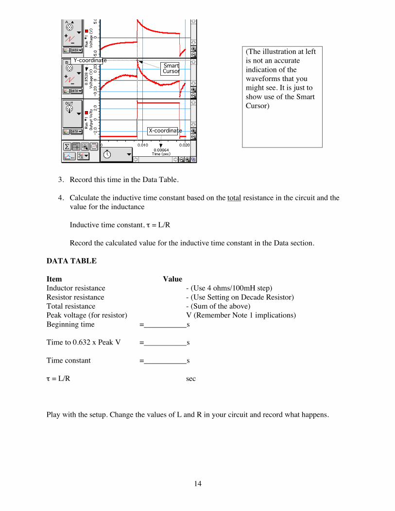
(The illustration at left is not an accurate indication of the waveforms that you might see. It is just to show use of the Smart Cursor)

3. Record this time in the Data Table.

4. Calculate the inductive time constant based on the total resistance in the circuit and the

value for the inductance

Inductive time constant, τ = L/R Record the calculated value for the inductive time constant in the Data section.

DATA TABLE Item Value Inductor resistance - (Use 4 ohms/100mH step) Resistor resistance - (Use Setting on Decade Resistor) Total resistance - (Sum of the above) Peak voltage (for resistor) V (Remember Note 1 implications) Beginning time =___________s Time to 0.632 x Peak V =___________s Time constant =___________s τ = L/R sec Play with the setup. Change the values of L and R in your circuit and record what happens.

X-coordinate

Y-coordinateSmart Cursor

15

QUESTIONS

1. How does the inductive time constant found in this experiment compare to the theoretical value given by τ = L/R? (Remember that R is the total resistance of the circuit and therefore must include the resistance of the coil as well as the resistance of the resistor.)

2. Does Kirchhoff’s Loop Rule hold at all times? Use the graphs to check it for at least three

different times: Does the sum of the voltages across the resistor and the inductor equal the source voltage at any given time?

Note 1: The signal generator may have some zero offset and/or some minor calibration

errors in the peak indications of each waveform. Therefore, compensate for these possible errors as much as possible, using the Smart Cursor feature to make more precise measurements.

1) Measure and Record Baseline Offset 2) Record Peak Level

3) Add or subtract the Offset to get the “True” peak-to-peak amplitude

4) Multiply this by 0.632 to get the voltage level above as appropriate

5) Add or subtract Offset to the above level as appropriate.

6) Move the Smart Cursor crosshair so the above value is displayed on the Voltage

scale at the same time that it is centered on the data curve. Record the time indicated on the Time Scale.

7) Now move the Smart Cursor to the left and align the vertical crosshair to the

beginning of the rise from Baseline. Record the number displayed in the Time Scale.

8) Subtract start time of curve from end time to get TC value. Remember to include

appropriate significant digits.

9) Compare the Experimental TC value to the Computed TC value.

10) Report % error.