experiment no.1: ellipsometry room no.: 145 (colloids …manuals-2016.pdfcl 610 – experimental...
TRANSCRIPT
CL 610 – Experimental Methods
Experiment No.1: Ellipsometry
Room No.: 145 (Colloids and
Nanomaterials Lab)
Lab Manual
Department of Chemical Engineering,
Indian Institute of Technology, Bombay
Thin film formation by spin coating and thickness measurement by
Ellipsometry
Objective
To make a thin-film of polymer by spin coating and measure thickness of the polymer thin film
by Ellipsometry.
Introduction
Optical measurement techniques are normally non-invasive. These techniques do not involve any
physical contact with the surface and do not destruct the surface. This is a lucrative property of a
measurement technique on nano-scale. Several optical measurement techniques based on the
reflection or transmissions of light from a surface are interferometry, reflectometry and
ellipsometry. There are three different types of ellipsometry, namely scattering, transmission and
reflection ellipsometry. This experiment deals with the reflection ellipsometry only. One of the
applications is in the semiconductor industry, which deals with a thin layer of SiO2 on a silicon
wafer. To ensure the thickness of this film, process engineers use ellipsometry to measure the
film thickness of sample wafers. Ellipsometry is known for the high accuracy when measuring
very thin film, with a thickness in the Angström scale or below. Other applications of
ellipsometry involve determination of the refractive index, the surface roughness or the
uniformity of a sample and more.
Theory
a) Spin coating
Spin coating is one of the standard methods for obtaining uniformly thick dielectric films.
The substrate on which the desired material is to be coated is mounted on the spin coater and
held by vacuum. The polymer dissolved in a suitable volatile solvent or synthesized in solution is
poured on the substrate and it is spun at high speeds of the order of few thousand rpm. Clearly
the film thickness will increase with the increase in concentration in solution and will reduce
with the increase in spin speed. But other factors like viscosity, volatility of the solvent used,
humidity of the environment, etc. also matter [1, 3].
The mechanism of film formation can be split into 2 stages. The first stage involves the
interplay between the centrifugal and viscous forces followed by evaporation. Meyerhofer (1978)
predicted the final thickness, hf in terms several solution parameters [1, 3] as given by the
following equation:
13
2(1 )
f
eh x
x K
Where e and K are the evaporation and flow constants defined below and x is the effective solid
constant of the solution.
2
3
e C
K
Where ω is the rotation rate, ρ is the density of the solution, η is its viscosity and C is
a proportionality constant that depends on whether airflow above the surface is laminar or
turbulent and on the diffusivity of the solvent molecules in air.
Substituting e and K in the equation for hf [1, 3, 6] we can see that the thickness varies linearly
as the inverse square root of spinning speed, when other parameters remain the same.
This is the relationship which we will verify experimentally.
tconsh f
tan
b) Ellipsometry
Ellipsometry is primarily used to determine film thickness and optical constants. However, it is
also applied to characterize composition, crystallinity, roughness, doping concentration, and
other material properties associated with a change in optical response.
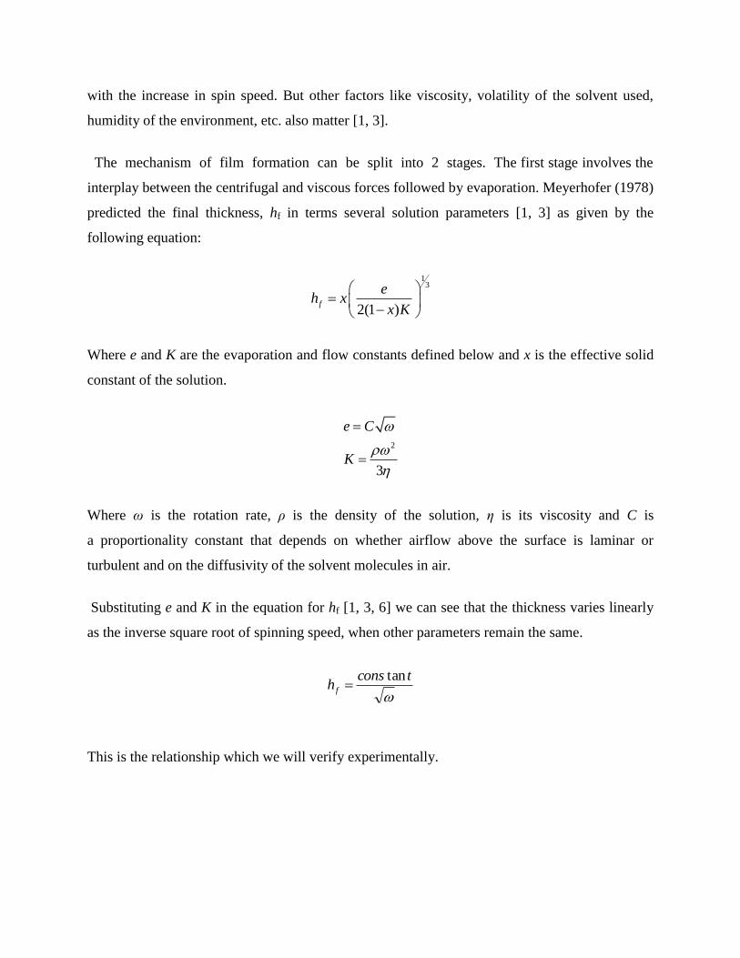
Light can be represented as a transverse electromagnetic wave made up of mutually
perpendicular, fluctuating electric and magnetic fields. The left side of the following diagram
shows the electric field in the xy plane, the magnetic field in the xz plane and the propagation of
the wave in the x direction. The right half shows a line tracing out the electric field vector as it
propagates. Traditionally, only the electric field vector is dealt with because the magnetic field
component is essentially the same.
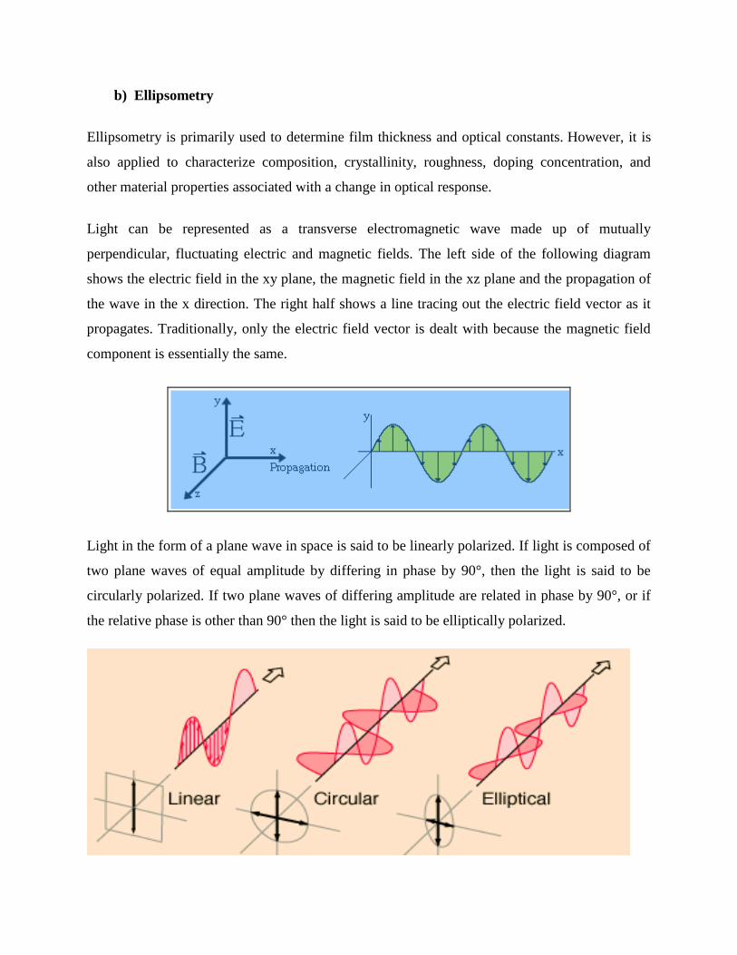
Light in the form of a plane wave in space is said to be linearly polarized. If light is composed of
two plane waves of equal amplitude by differing in phase by 90°, then the light is said to be
circularly polarized. If two plane waves of differing amplitude are related in phase by 90°, or if
the relative phase is other than 90° then the light is said to be elliptically polarized.
The polarization change is represented as an amplitude ratio, Ψ, and the phase difference, Δ [2].
The measured response depends on optical properties and thickness of individual materials.
Ellipsometry measures the interaction between light and material.
When light enters a different medium the dielectric constant of the medium changes the
electrical field strength. As light is electromagnetic wave, in a different dielectric medium, it
changes it’s velocity for which it changes its trajectory and wavelength. When a polarized light
beam falls at the interface of two dielectric media, its electric vector can be separated into two
orthogonal components parallel and perpendicular to the plane of incidence (p and s components
respectively). When these components traverse through the medium and undergo reflection and
refraction, there is a change in the polarization of the light which is a function of amplitude ratio
and phase difference of these components. The change in polarization is the ellipsometry
measurement, commonly written as:
tan exp(i )p
s
R
R
Where tanp
s
R
R
which again can be derived from Maxwell’s theory as a function of total
reflectance R, refractive index, incident angle, wavelength of the incident light and thickness of
the film. Out of these parameters except the thickness other parameters are constant for a given
system, thus calculable (or can be found in literature).
For a transparent film the Cauchy relationship [2] is typically given as:
2 4( )
B Cn A
Where, the three terms are adjusted to match the refractive index for the material.
So in the model the only unknown variable remains, is thickness for the film, as the total
reflectance is also a function of refractive index and incident angle.
The Ellipsometer experimentally measures the amplitude ratio vs. wavelength of light and phase
difference vs. wavelength of light which is the fitted with the theoretically obtained amplitude
ratio vs. wavelength of light and phase difference vs. wavelength of light, having the fitting
parameters A, B, C (Cauchy parameters) and hf. These parameters are fitted to obtain the film
thickness.
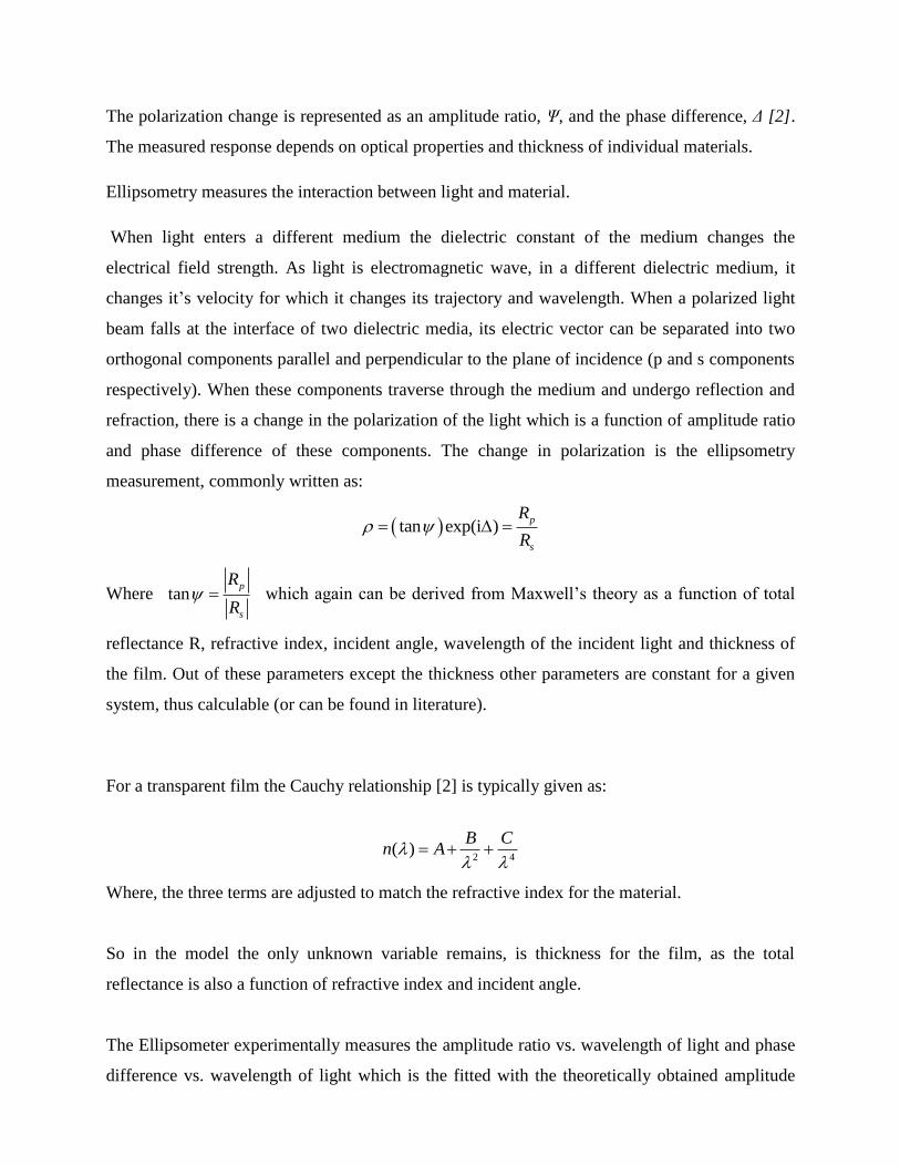
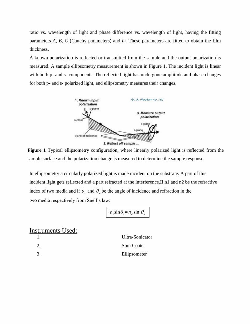
A known polarization is reflected or transmitted from the sample and the output polarization is
measured. A sample ellipsometry measurement is shown in Figure 1. The incident light is linear
with both p- and s- components. The reflected light has undergone amplitude and phase changes
for both p- and s- polarized light, and ellipsometry measures their changes.
In ellipsometry a circularly polarized light is made incident on the substrate. A part of this
incident light gets reflected and a part refracted at the interference.If n1 and n2 be the refractive
index of two media and if 1 and 2 be the angle of incidence and refraction in the
two media respectively from Snell’s law:
Instruments Used: 1. Ultra-Sonicator
2. Spin Coater
3. Ellipsometer
Figure 1 Typical ellipsometry configuration, where linearly polarized light is reflected from the
sample surface and the polarization change is measured to determine the sample response
1n sin 1 = 2n sin 2
Chemicals Used:
1. Polystyrene solution
2. Silicon wafer
3. Toluene
4. Milli-Q-water
Procedure:
1. Polystyrene solution with toluene is prepared
2. Silicon wafer is mounted on the chuck of spin coater and vacuum is on to keep the
sample in place
3. Sample is placed on the wafer and rotational speed is set in a desired value.
4. Wafer is taken out and thickness is measured in Ellipsometer
5. Thickness measuring software is initialized and then sample is loaded.
6. Then beam alignment is done and then data is taken. Depolarisation is also measured.
7. Once data is collected from spectroscopic scan, data is fitted with Cauchy model. Fitting
is continued till the MSE is less than 20%. To reduce the MSE, higher order terms in
Cauchy equation is taken into account.
8. If there is depolarisation in sample, data collected in that range (wave length range) is
removed and rest of the data are fitted with theoretical model.
References:
1. David B. Hall, Patrick Underhill and John M. Torkelson,’ Spin Coating of Thin and
Ultrathin Polymer Films’, Polymer engineering and Science, December 1998, Vol. 38,
No. 12
2. http://www.jawoollam.com/tutorial_1.html
3. Niranjan Sahu, B Parija, and S Panigrahi, ‘Fundamental understanding and modeling of
spin coating process’, Indian J.Physics, 83(4) 493-502 (2009)
4. A G Emsile, F T Bonner and L G Peek J. Appl. Phys. 29 858 (1958)
5. C J Lawrence and W Zhou Journal of Non-Newtonian Fluid Mechanics 39137 (1991)
6. http://www.cise.columbia.edu/clean/process/spintheory.pdf
CL 610 – Experimental Methods
Experiment No. 2: Karl Fischer
Room No.: 227 (Organic Processing Lab)
Lab Manual
Department of Chemical Engineering,
Indian Institute of Technology, Bombay
Measurement of percentage moisture using Karl Fischer volumetric titration
in a sample of unknown moisture content
Aim:
Determine the percent moisture in Potassium Chloride and Glycerol samples using Karl Fischer
volumetric titration.
Introduction:
Pioneered by a German chemist, Karl Fischer titration has achieved to be established as the most
important method for determining water and humidity. With the KF titration both free and bound
water can be determined, e.g. surface water on crystals or the water contained inside them. The
method works over a wide concentration range from ppm up to 100% and supplies reproducible
and correct results. Karl Fischer titration is used in determining the water in diesel fuel and
gasoline, silicone oil, liquid ammonia etc. and for the analysis of edible fats and oils.
Apparatus and Instrument: The experiment is performed in organic process lab.
Glassware – Beakers, Titration flask with magnetic stirrer
Karl Fischer Titrator, Weighing balance
Chemicals:
Karl Fischer reagent,
Karl Fischer grade dry methanol
Di-sodium tartrate dihydrate (purified)
Samples (KCl and Glycerol)
Principle:
When developing his new analytical method Karl Fischer took into account the well known
Bunsen reaction, which is used for the determination of sulfur dioxide in aqueous solutions:
SO2 + I2 + 2 H2O → H2SO4 + 2 HI
To determine the titer of Karl Fischer reagent which is measured as mg of water per ml (mg
H2O/ml of KF reagent) of Karl Fischer reagent. In Karl Fischer volumetric titration, iodine is
added to solvent containing the sample by a burette. Moisture is calculated on the basis of the
volume of Karl Fischer reagent consumed.
Volumetric titration is recommended for determination of water content in the range of 0.1% to
100%.
Volumetric Karl-Fischer titration:
The volumetric Karl Fischer titration is based on the stoichiometric principle that 1 mole of
iodine reacts with 1 mole of water. Water and iodine are consumed in 1:1 ratio in the following
reaction
I2+ SO2 + H2O + 3Base + CH3OH → 2Base HI + Base HSO4CH3
When all the moisture present is consumed the excess iodine present is detected
voltammetrically by the titrator electrode. The system controls the current voltage detection. A
constant current of 1-30µA is applied to the two platinum electrodes. If the titration solution has
a high moisture, a polarization voltage of 300-500mV will be produced. As the titration
continues and the end point is near, the voltage suddenly drops to 10-50 mV. In volumetric
analysis the endpoint is considered to have reached after the voltage has remained at this level
for a specific period of time. In commercial titration systems, this period is 30-60 seconds.
The moisture present in the sample is then calculated on the basis of concentration of iodine in
Karl Fischer reagent and the amount of Karl Fischer reagent consumed in the titration.
Procedure:-
1. Put 50 ml KF-grade methanol in the flask which has been well dried in hot air oven
overnight.
2. Fill the desiccant tubes with silica gel and molecular sieves and place at the appropriate
positions on the titration flask.
3. Place KF dispenser and platinum electrode opposite to one another at the titration flask.
4. Carry out a neutralization step to remove all the moisture that may have been added along
with the solvent.
5. Standardization: Add a fixed amount of Millipore water into the flask to know the
concentration factor of KF reagent. The amount of water should be 25 mg to 250mg.
6. Add KCl sample containing unknown amount of moisture in the flask and titrated. The
endpoint reaches when the voltage remains at 10-20 mV for some time.
7. Repeat the titrations for each sample thrice and note the amount.
8. Wait till the end point is detected electrically by the system and titration stops.
9. Note the volume of KF reagent consumed and moisture percentage.
10. Repeat the above steps to determine the moisture of anhydrous Glycerol sample.
11. Repeat the above steps for determination of moisture with hydrated samples of KCl and
Glycerol.
12. Calculate the moisture content using the concentration factor noted by standardization.
Calculation:
Concentration factor = S
Leak rate = L
Weight of Millipore water
Used in standardization = W
Blank volume = B
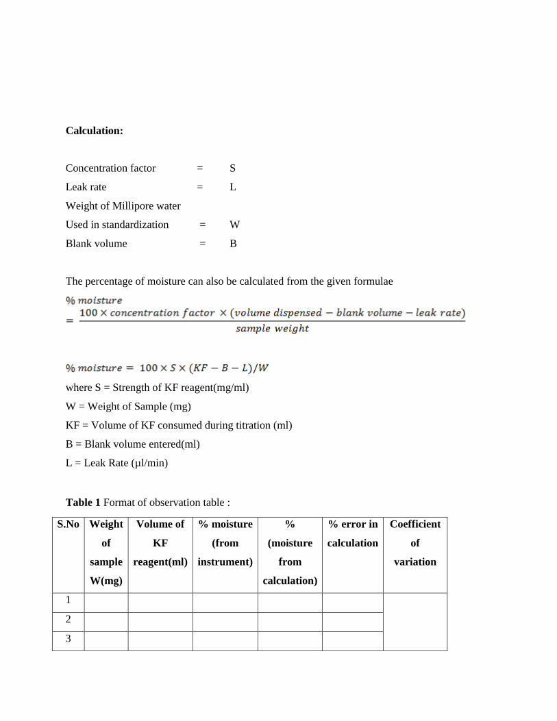
The percentage of moisture can also be calculated from the given formulae
where S = Strength of KF reagent(mg/ml)
W = Weight of Sample (mg)
KF = Volume of KF consumed during titration (ml)
B = Blank volume entered(ml)
L = Leak Rate (µl/min)
Table 1 Format of observation table :
S.No Weight
of
sample
W(mg)
Volume of
KF
reagent(ml)
% moisture
(from
instrument)
%
(moisture
from
calculation)
% error in
calculation
Coefficient
of
variation
1
2
3
Sources of error:
1. For very low moisture content the low sample quantity the burette resolution is not
suitable to reproduce the results.
2. Potassium Chloride which has low solubility in methanol which is used as solvent in
this method cannot dissolve the consecutive samples, and hence calculates low
moisture.
References:
1. Eugen Scholz Reagents for Karl Fischer Titration,
Sigma-Aldrich/Riedel-de-Haën,2001
2. Peter Bruttel, Regina Schlink, Water Determination by Karl Fischer Titration
CL 610 – Experimental Methods
Experiment No. 3: High Performance
Thin Layer Chromatography
Room No.: 225 (Organic Processing Lab)
Lab Manual
Department of Chemical Engineering,
Indian Institute of Technology, Bombay
2
High Performance Thin Layer Chromatography
3.1. Aim: To measure the unknown concentration of Benzophenone and Benzhydrol in a
mixture.
3.2. Introduction
Chromatography is a technique which is mostly used for separating and identifying compounds
in a mixture. It is a very useful technique in industry where it is used for large scale separation
and purification of various products and intermediates in a chemical reaction.
All chromatographic techniques require a stationary phase and a mobile phase. The separation of
components in chromatography is based on the differential adsorption of components onto the
stationary phase or the mobile phase. There are several different types of chromatography which
are used – i.e. paper chromatography; high performance thin layer chromatography (HPTLC);
gas chromatography (GC); liquid chromatography (LC); high performance liquid
chromatography (HPLC); ion exchange chromatography; and gel permeation or gel filtration
chromatography.
Thin Layer Chromatography (TLC) is an extremely useful technique for monitoring reactions,
identify compounds given in a mixture and determine the purity of a substance. High
Performance Thin Layer Chromatography (HPTLC) is an enhanced form of thin layer
chromatography (TLC). A number of enhancements can be made to the basic method of thin
layer chromatography to automate different steps, to increase the resolution achieved and to
allow more accurate quantitative measurements. Automation allows overcoming the uncertainty
in droplet size and position when the sample is applied to the TLC plate by hand.
3
3.3. Theory
3.3.1. Stationary phase:
TLC uses a stationary phase, usually alumina or silica supported on an inert base such as glass,
aluminum foil or insoluble plastic. The mixture to be separated is ‘spotted’ at the bottom of the
TLC plate and allowed to dry. The plate is placed in a closed vessel containing solvent (the
mobile phase) so that the liquid level is below the spot.
3.3.2. Mobile phase:
The mobile phase is a solvent whose polarity is chosen according to the requirements. The
solvent ascends the plate by capillary action, the liquid filling the spaces between the solid
particles. This technique is usually done in a closed vessel to ensure that the atmosphere is
saturated with solvent vapour and that evaporation from the plate is minimised before the run is
complete. The plate is removed when the solvent front approaches the top of the plate and the
position of the solvent front recorded before it is dried (this allows the Rf value to be calculated).
3.3.3. Principle of separation:
In chromatography, the components of a mixture get differentially partitioned between the
stationary phase and the mobile phase depending on their interaction with the adsorbent. This
results in differential rates of migration of various components in a mixture. At any given time, a
particular analyte molecule is either in the mobile phase, moving along at its velocity, or in the
stationary phase and not moving at all in the downstream direction. The sorption–desorption
process occurs many times as the molecule moves through the bed. The ratio of the equilibrium
concentration of an analyte in the stationary phase to that in the mobile phase is called the
distribution constant or the partition co-efficient: Ka.
Ka = Cs/Cm
Where Cs is the equilibrium concentration of the analyte in the stationary phase and Cm is the
equilibrium concentration of the analyte in the mobile phase. As the chromatography proceeds,
it partitions itself between the two phases depending on its distribution constant. A lower
partition co-efficient means that the analyte will migrate faster and spend less time in the
stationary phase.
4
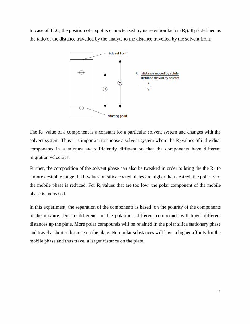
In case of TLC, the position of a spot is characterized by its retention factor (Rf). Rf is defined as
the ratio of the distance travelled by the analyte to the distance travelled by the solvent front.
The Rf value of a component is a constant for a particular solvent system and changes with the
solvent system. Thus it is important to choose a solvent system where the Rf values of individual
components in a mixture are sufficiently different so that the components have different
migration velocities.
Further, the composition of the solvent phase can also be tweaked in order to bring the the Rf to
a more desirable range. If Rf values on silica coated plates are higher than desired, the polarity of
the mobile phase is reduced. For Rf values that are too low, the polar component of the mobile
phase is increased.
In this experiment, the separation of the components is based on the polarity of the components
in the mixture. Due to difference in the polarities, different compounds will travel different
distances up the plate. More polar compounds will be retained in the polar silica stationary phase
and travel a shorter distance on the plate. Non-polar substances will have a higher affinity for the
mobile phase and thus travel a larger distance on the plate.
5
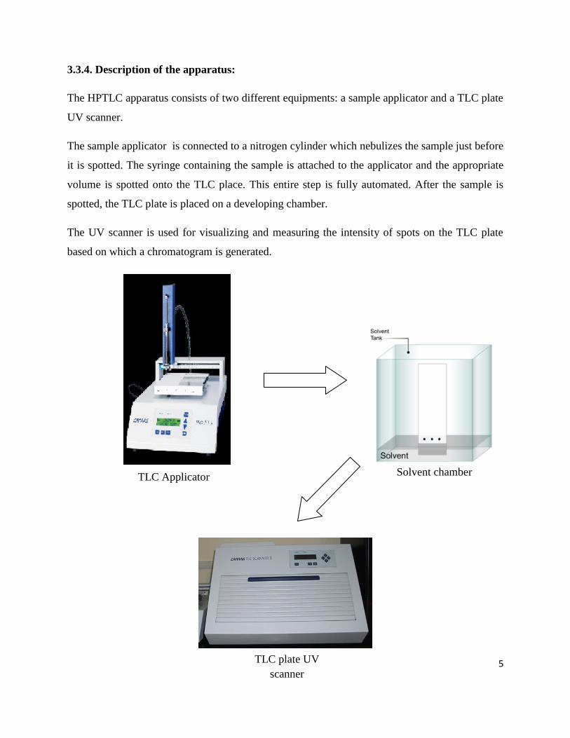
3.3.4. Description of the apparatus:
The HPTLC apparatus consists of two different equipments: a sample applicator and a TLC plate
UV scanner.
The sample applicator is connected to a nitrogen cylinder which nebulizes the sample just before
it is spotted. The syringe containing the sample is attached to the applicator and the appropriate
volume is spotted onto the TLC place. This entire step is fully automated. After the sample is
spotted, the TLC plate is placed on a developing chamber.
The UV scanner is used for visualizing and measuring the intensity of spots on the TLC plate
based on which a chromatogram is generated.
TLC Applicator Solvent chamber
TLC plate UV scanner
6
3.3.5. Apparatus used: TLC Plate, Applicator, Glass developing chamber, TLC UV Scanner,
Syringe, Beakers, Measuring cylinder, Sample bottles.
3.3.6. Chemicals used: Benzophenone, Benzhydrol, Methanol, Hexane, Toluene.
3.4. Experimental Procedure:
1. Two standard solutions of 150 ppm Benzophenone and 2500 ppm Benzhydrol each was
prepared in 5ml of methanol.
2. Mixtures of Benzophenone and Benzhydrol in unknown proportions were also prepared.
3. 30ml of developing solvent containing Hexane-Toluene in a ratio of 30:70 was prepared
and poured in the developing chamber.
4. The HPTLC instrument (applicator) was started and various parameters like Plate width,
Band width, Band pitch and start position were set. Based on these parameters the
number of tracks available on the TLC plate was calculated to be 13.
5. In the first five tracks, bands of pure Benzophenone solution, in the middle five tracks,
bands of pure Benzhydrol solution and in the last three tracks, bands of unknown samples
were loaded by entering different volumes of the samples in each track.
6. After applying the samples, the TLC plate was kept in the developing chamber containing
the solvent. The plate was removed when the solvent had covered 75% of the plate and
was dried with the help of a dryer.
7. The TLC plate was placed under a UV lamp for identification of the bands after they had
migrated.
8. The plate was then analyzed by using the TLC scanner in order to obtain the
chromatograms using the CAMAG software at 254nm wavelength. Each track was
separately analyzed and depending on the number of components present they showed
one or two peaks. By using the integration option the areas under the peaks were
obtained.
3.4.1. Preparation of standard solutions of Benzophenone and Benzhydrol:
5.94 mg of Benzophenone was dissolved in 50 ml of Methanol (density: 0.791 g/cc) to give a
solution of 150 ppm. 98.99 mg of Benzhydrol was dissolved in 50 ml of Methanol (density:
0.791 g/cc) to give a solution on 2500 ppm.
7
3.4.2. Parameters entered:
Plate width = 200 mm
Space between bands = 10 mm
Band width = 4 mm
Observations:
Start position = 10 mm
3.6. Calculations:
Determine the calibration factors for Benzophenone and Benzhydrol.
Report the unknown concentrations of these two in a mixture from the above plots (in
ppm).
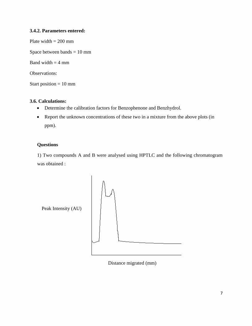
Questions
1) Two compounds A and B were analysed using HPTLC and the following chromatogram
was obtained :
Peak Intensity (AU)
Distance migrated (mm)
8
What parameters will you modify so as to get two distinct peaks in the chromatogram and a
merged peak?
2) You have a mixture of 3 compounds A, B and C. The Rf values of the compounds in different
solvent systems are given below:
Compound Name Solvent systems Hexane – Toluene
(Rf) Hexane – Water
(Rf) Hexane – Acetonitrile
(Rf) A 0.30 1 0.25 B 0.25 0.90 0.65 C 0.31 0.95 0.89
Which solvent system would you choose for separating the compounds? Give reasons.
3) A polar compound – X, when analysed on a TLC plate coated with silica using a solvent
system of Hexane and Toluene in a ratio of 3:10 gave a Rf value of 1. What modifications do you
suggest to decrease the Rf value using the same solvents Hexane and Toluene?
4) The minimum detection limit (MDL) of compounds A and B using HPTLC when scanned
using a UV scanner is 0.15 ug and 3.5 ug respectively. Which property of the compound would
determine the MDL? Explain w.r.t. the compounds A and B.
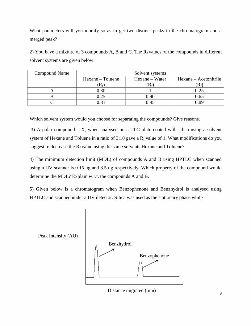
5) Given below is a chromatogram when Benzophenone and Benzhydrol is analysed using
HPTLC and scanned under a UV detector. Silica was used as the stationary phase while
Peak Intensity (AU)
Distance migrated (mm)
Benzhydrol
Benzophenone

9
Ethanol is now added to the mixture of Benzophenone and Benzhydrol. Assuming that ethanol
does not interact with either BP or BH, where would you expect to find the peak of ethanol when
the TLC place is scanned under a UV detector? Give reasons for your answer.
6) A student spots an unknown sample on a TLC plate. After developing in hexanes/ethyl acetate
50:50, he/she saw a single spot with an Rf of 0.55. Does this indicate that the unknown material
is a pure compound? Give reasons for your answer.
CL 610 – Experimental Methods
Experiment No. 4: Rheometry
Lab Name: Fluid Mechanics Lab
Lab Manual
Department of Chemical Engineering,
Indian Institute of Technology, Bombay
CL- 610 Experimental Methods
Experiment 4: Rheometer 2
4.1 Objective
To measure the viscosity of suspended silica particles and study the behaviour of the sample’s
relative viscosity as linear (Einstein equation) with volume fraction of suspended solids using
rheometer
4.2 Introduction
Rheology is the science of deformation and flow of matter under controlled testing
conditions. Flow and deformation are interdependent to each other. Rheology studies the
relationships between deformations and stresses in a material, which in general is moving or
flowing.
Viscosity, the tendency of a fluid to resist the applied stress, is one of the important properties
of fluid in the field of fluid mechanics. It is used in designing of pumps and piping, mixing
and agitation of dispersions and solutions, coatings, adhesives and other chemical processes.
The viscosity of fluid varies with introduction of dispersed phase, such as emulsions and
slurries, and also depends on physical (size and concentration) and chemical properties of
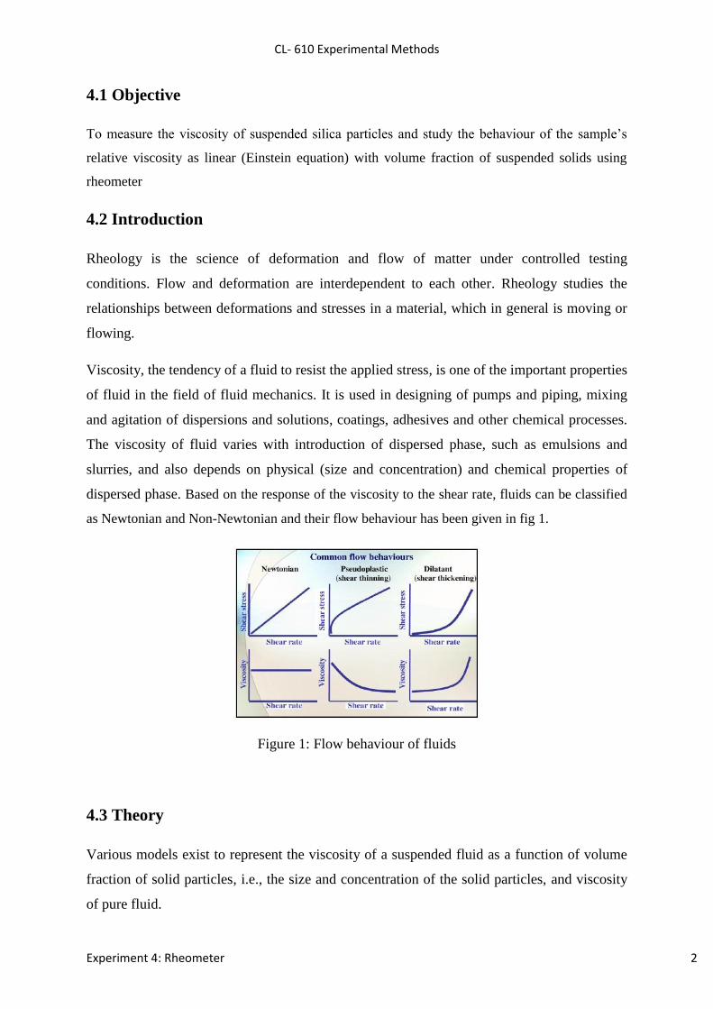
dispersed phase. Based on the response of the viscosity to the shear rate, fluids can be classified
as Newtonian and Non-Newtonian and their flow behaviour has been given in fig 1.
Figure 1: Flow behaviour of fluids
4.3 Theory
Various models exist to represent the viscosity of a suspended fluid as a function of volume
fraction of solid particles, i.e., the size and concentration of the solid particles, and viscosity
of pure fluid.
CL- 610 Experimental Methods
Experiment 4: Rheometer 3
4.3.1 Einstein Model (Linear):
It may be used for extremely low concentrations of fine particles and particles are considered as spherical and there is no interaction among them.
(4.1)
Where and = Viscosity of particle suspended fluid and pure fluid respectively [Pa.s],
= Volume fraction of suspended solid particles in the fluid and = Constant
4.3.2 Rheometer Operating Principle
Common characteristic of all rheometer is the measure of two physical quantities: one is a
dynamic quantity (i.e. a force, torque) and the other is a kinematic quantity (i.e. a velocity,
shear rate, flow rate, time). One of the two quantities is directly controlled (or set) by the
instrument.
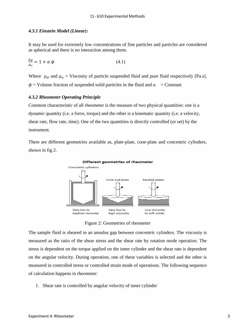
There are different geometries available as, plate-plate, cone-plate and concentric cylinders,
shown in fig 2.
Figure 2: Geometries of rheometer
The sample fluid is sheared in an annulus gap between concentric cylinders. The viscosity is
measured as the ratio of the shear stress and the shear rate by rotation mode operation. The
stress is dependent on the torque applied on the inner cylinder and the shear rate is dependent
on the angular velocity. During operation, one of these variables is selected and the other is
measured in controlled stress or controlled strain mode of operations. The following sequence
of calculation happens in rheometer:
1. Shear rate is controlled by angular velocity of inner cylinder
CL- 610 Experimental Methods
Experiment 4: Rheometer 4
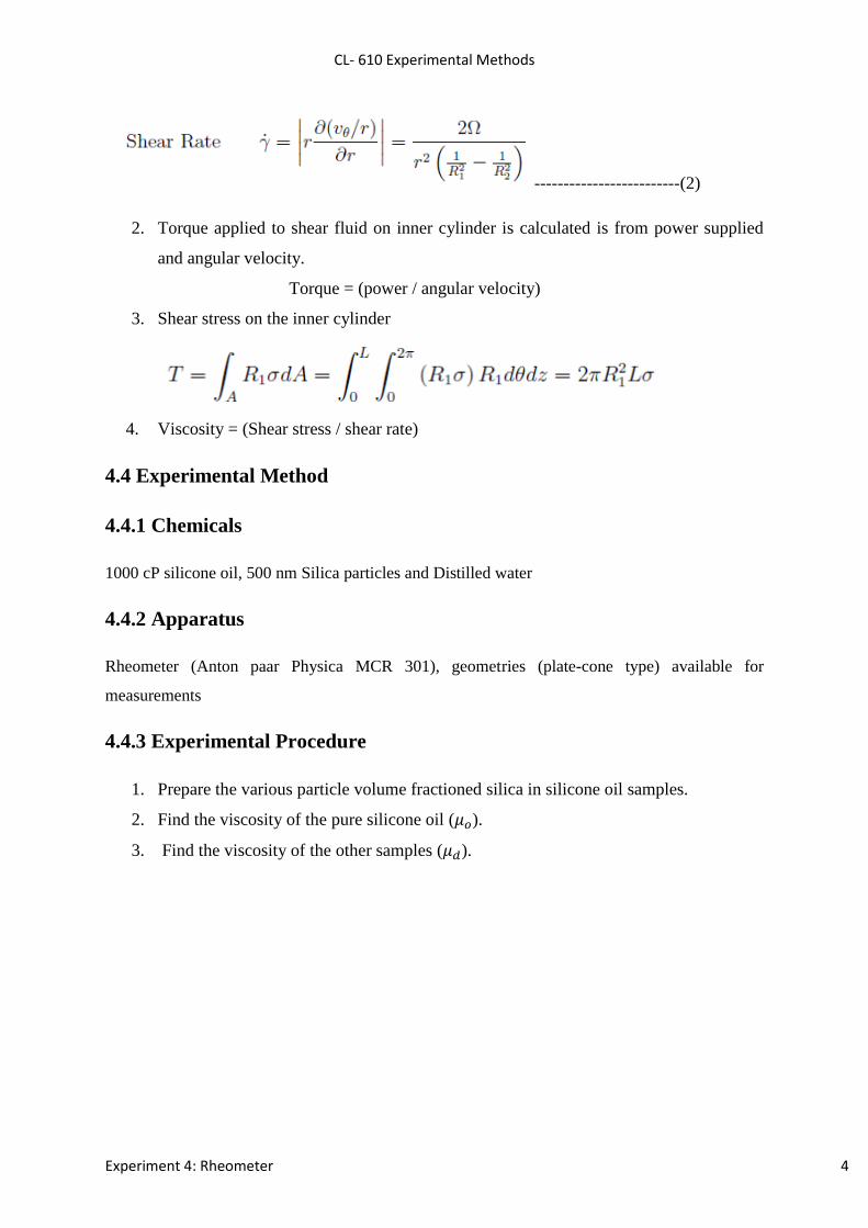
-------------------------(2)
2. Torque applied to shear fluid on inner cylinder is calculated is from power supplied
and angular velocity.
Torque = (power / angular velocity)
3. Shear stress on the inner cylinder
4. Viscosity = (Shear stress / shear rate)
4.4 Experimental Method
4.4.1 Chemicals
1000 cP silicone oil, 500 nm Silica particles and Distilled water
4.4.2 Apparatus
Rheometer (Anton paar Physica MCR 301), geometries (plate-cone type) available for
measurements
4.4.3 Experimental Procedure
1. Prepare the various particle volume fractioned silica in silicone oil samples.
2. Find the viscosity of the pure silicone oil ( ).
3. Find the viscosity of the other samples ( ).
CL- 610 Experimental Methods
Experiment 4: Rheometer 5
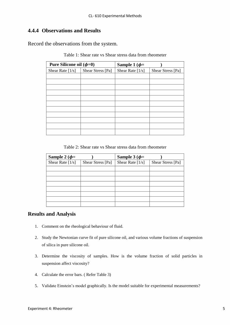
4.4.4 Observations and Results
Record the observations from the system.
Table 1: Shear rate vs Shear stress data from rheometer
Pure Silicone oil ( =0) Sample 1 ( = ) Shear Rate [1/s] Shear Stress [Pa] Shear Rate [1/s] Shear Stress [Pa]
Table 2: Shear rate vs Shear stress data from rheometer
Sample 2 ( = ) Sample 3 ( = ) Shear Rate [1/s] Shear Stress [Pa] Shear Rate [1/s] Shear Stress [Pa]
Results and Analysis
1. Comment on the rheological behaviour of fluid.
2. Study the Newtonian curve fit of pure silicone oil, and various volume fractions of suspension
of silica in pure silicone oil.
3. Determine the viscosity of samples. How is the volume fraction of solid particles in
suspension affect viscosity?
4. Calculate the error bars. ( Refer Table 3)
5. Validate Einstein’s model graphically. Is the model suitable for experimental measurements?
CL- 610 Experimental Methods
Experiment 4: Rheometer 6
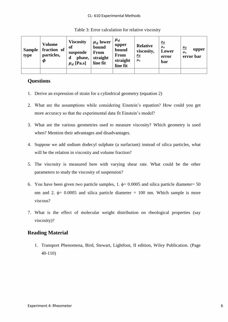
Table 3: Error calculation for relative viscosity
Sample type
Volume fraction of particles,
Viscosity of suspended phase, [Pa.s]
lower bound From straight line fit
upper bound From straight line fit
Relative viscosity,
Lower error bar
upper
error bar
Questions
1. Derive an expression of strain for a cylindrical geometry (equation 2)
2. What are the assumptions while considering Einstein’s equation? How could you get
more accuracy so that the experimental data fit Einstein’s model?
3. What are the various geometries used to measure viscosity? Which geometry is used
when? Mention their advantages and disadvantages.
4. Suppose we add sodium dodecyl sulphate (a surfactant) instead of silica particles, what
will be the relation in viscosity and volume fraction?
5. The viscosity is measured here with varying shear rate. What could be the other
parameters to study the viscosity of suspension?
6. You have been given two particle samples, 1. = 0.0005 and silica particle diameter= 50
nm and 2. = 0.0005 and silica particle diameter = 100 nm. Which sample is more
viscous?
7. What is the effect of molecular weight distribution on rheological properties (say
viscosity)?
Reading Material
1. Transport Phenomena, Bird, Stewart, Lightfoot, II edition, Wiley Publication. (Page
40-110)
CL 610 – Experimental Methods
Expt.No.5
Rotating Disc Voltametry
Room No.: 227 (Organic Processing Lab)
Lab Manual
Department of Chemical Engineering,
Indian Institute of Technology, Bombay
Rotating Disk Voltammetry Aim: To find out the diffusion coefficient and mass transfer coefficients of K3[Fe(CN)6] using Rotating Disk Electrode. Experimental Apparatus: 1) Pine Instrument Company AFCBP1 Bipotentiostat 2) Pine Instrument Company ASWCV2 Pine ChemTM software package 3) Platinum rotated disk electrode. 4) Pine Instrument Company MSRX rotator 5) Three electrode cell. 6) Platinum counter electrode. 7) Saturated Calomel Electrode (SCE) reference electrode. Reagents & Chemicals: 10 mM Potassium Ferricyanide K3 [Fe(CN)6] in 1M Potassium Nitrate as supporting electrolyte. Theory:
A general description of the term voltammetry is an electrochemical technique that involves controlling the potential of an electrode while simultaneously measuring the current flowing through that electrode. The electrode in question is usually called the working electrode in order to distinguish it from other electrodes that are present in the electrochemical cell.
Voltammetry is usually performed by connecting an electrochemical potentiostat
to an electrochemical cell. The cell contains a test solution and three electrodes: working, reference and auxiliary. Special electronic circuitry within the potentiostat permits the working electrode potential to be connected with respect to the reference electrode without any appreciable current flowing through the reference electrode. Rather, the current is forced to flow between the working and auxiliary electrode as such a magnitude, that the desired potential is maintained between the working and reference electrodes. This unusual arrangement has two principal benefits. First, the reference electrode is protected from internal electrochemical changes caused by current flow. Second, measurement errors related to the resistance of the test solution are kept to minimum. There are quite a number of voltammetry techniques. Each differs in the precise manner that the working electrode potential is changed during the experiment. In some techniques, a potential sweep is applied to the working electrode, in others: a sudden potential step or complex pulse sequence is used. Another distinguishing feature is whether or not the solution is moving with respect to the surface of the working electrode.
In most cases, the solution is motionless, but there exist many hydrodynamic methods in which solution moves toward the electrode along a well-defined flow pattern. The rotated disk electrode is an example of a hydrodynamic method.
The analyte used in this experiment is the ferricyanide anion, Fe(CN)6
3- which contains an iron atom in the +3 oxidation state. At the surface of the working electrode, a single electron can be added to the ferricyanide anion. This causes it to be reduced to the ferrocyanide anion, Fe(CN)6
4- which contains an iron atom in the +2 oxidation state. This simple one electron exchange between the analyte and the electrode is very
well behaved, and it is reversible. This means that the analyte can be easily reduced to Fe(CN)6
3- again. A pair of analytes differing only in oxidation state is known as redox couple. The
electrochemical half-reaction for the Fe(CN)63- /Fe(CN)6
4- redox couple can be written as follows:
Fe(CN)6
3- + e ------> Fe(CN)64-...........(1)
The formal potential associated with this half-reaction is near +400 mV vs the
normal hydrogen electrode (NHE).If the working electrode is held at a potential more positive than +40 mV, then the analyte tends to be oxidized to the Fe(CN)6
3- form. This oxidation at the working electrode causes an anodic current to flow (i.e., electrons go into the electrode from the solution). At potentials more negative than +400 mV, the analyte will be reduced to Fe(CN)6
4-. This reduction at the working electrode causes a cathodic current to flow (i.e., electrons flow out the electrode into the solution). Rotated Disc Voltammetry:
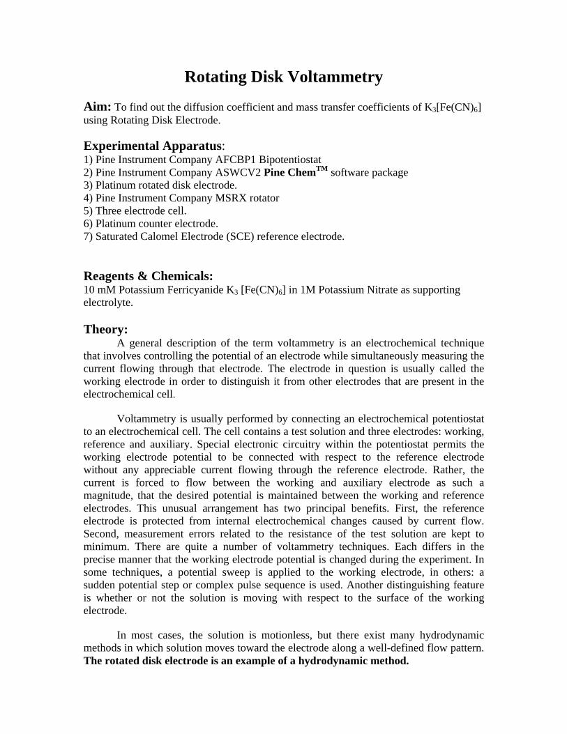
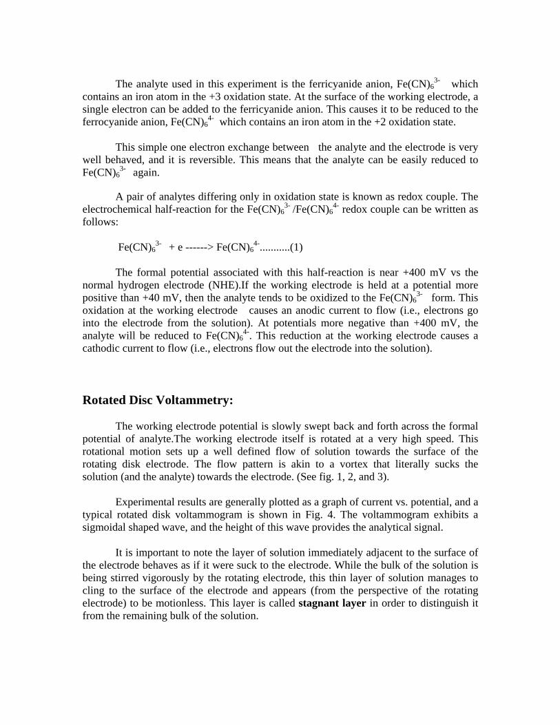
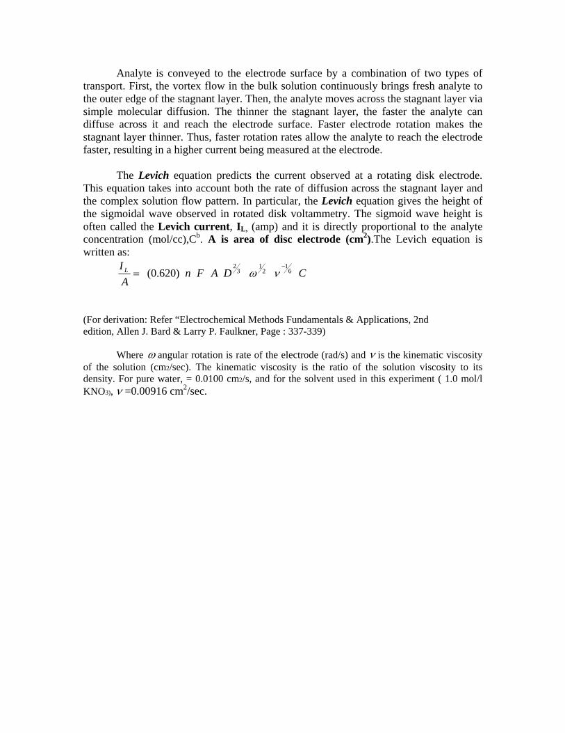
The working electrode potential is slowly swept back and forth across the formal potential of analyte.The working electrode itself is rotated at a very high speed. This rotational motion sets up a well defined flow of solution towards the surface of the rotating disk electrode. The flow pattern is akin to a vortex that literally sucks the solution (and the analyte) towards the electrode. (See fig. 1, 2, and 3).
Experimental results are generally plotted as a graph of current vs. potential, and a
typical rotated disk voltammogram is shown in Fig. 4. The voltammogram exhibits a sigmoidal shaped wave, and the height of this wave provides the analytical signal.
It is important to note the layer of solution immediately adjacent to the surface of
the electrode behaves as if it were suck to the electrode. While the bulk of the solution is being stirred vigorously by the rotating electrode, this thin layer of solution manages to cling to the surface of the electrode and appears (from the perspective of the rotating electrode) to be motionless. This layer is called stagnant layer in order to distinguish it from the remaining bulk of the solution.
Analyte is conveyed to the electrode surface by a combination of two types of transport. First, the vortex flow in the bulk solution continuously brings fresh analyte to the outer edge of the stagnant layer. Then, the analyte moves across the stagnant layer via simple molecular diffusion. The thinner the stagnant layer, the faster the analyte can diffuse across it and reach the electrode surface. Faster electrode rotation makes the stagnant layer thinner. Thus, faster rotation rates allow the analyte to reach the electrode faster, resulting in a higher current being measured at the electrode.
The Levich equation predicts the current observed at a rotating disk electrode.
This equation takes into account both the rate of diffusion across the stagnant layer and the complex solution flow pattern. In particular, the Levich equation gives the height of the sigmoidal wave observed in rotated disk voltammetry. The sigmoid wave height is often called the Levich current, IL, (amp) and it is directly proportional to the analyte concentration (mol/cc),Cb. A is area of disc electrode (cm2).The Levich equation is written as:
CDAFnAI L 6
12
13
2)620.0(
−= νω
(For derivation: Refer “Electrochemical Methods Fundamentals & Applications, 2nd
edition, Allen J. Bard & Larry P. Faulkner, Page : 337-339)
Where ω angular rotation is rate of the electrode (rad/s) and ν is the kinematic viscosity of the solution (cm2/sec). The kinematic viscosity is the ratio of the solution viscosity to its density. For pure water, = 0.0100 cm2/s, and for the solvent used in this experiment ( 1.0 mol/l KNO3), ν =0.00916 cm2/sec.
Experimental Procedure: 1) Prepare all the solutions: 10mM K3[Fe(CN)6] and 1M KNO3 as supporting electrolyte. 2) Equip a clean electrochemical cell with an SCE reference electrode and a platinum auxiliary electrode. Carefully mount the platinum disk working electrode in the rotator and then lower it into the cell. 3) Fill the electrochemical cell with the Analyte Solution. If desired, the oxygen in the cell may be purged by first bubbling nitrogen through the solution and then continuously blanketing the solution with a steady flow of nitrogen for the duration of the experiment. Oxygen is unlikely to interfere with this experiment, however. 4) Make proper connections to already placing all the three electrodes in the electrolytic cell which is filled with electrolyte (10mM K3[Fe(CN)6] and 1M KNO3 ). a) Reference electrode: Calomel Electrode. b) Working electrode: Platinum Electrode. c) Counter electrode: Platinum
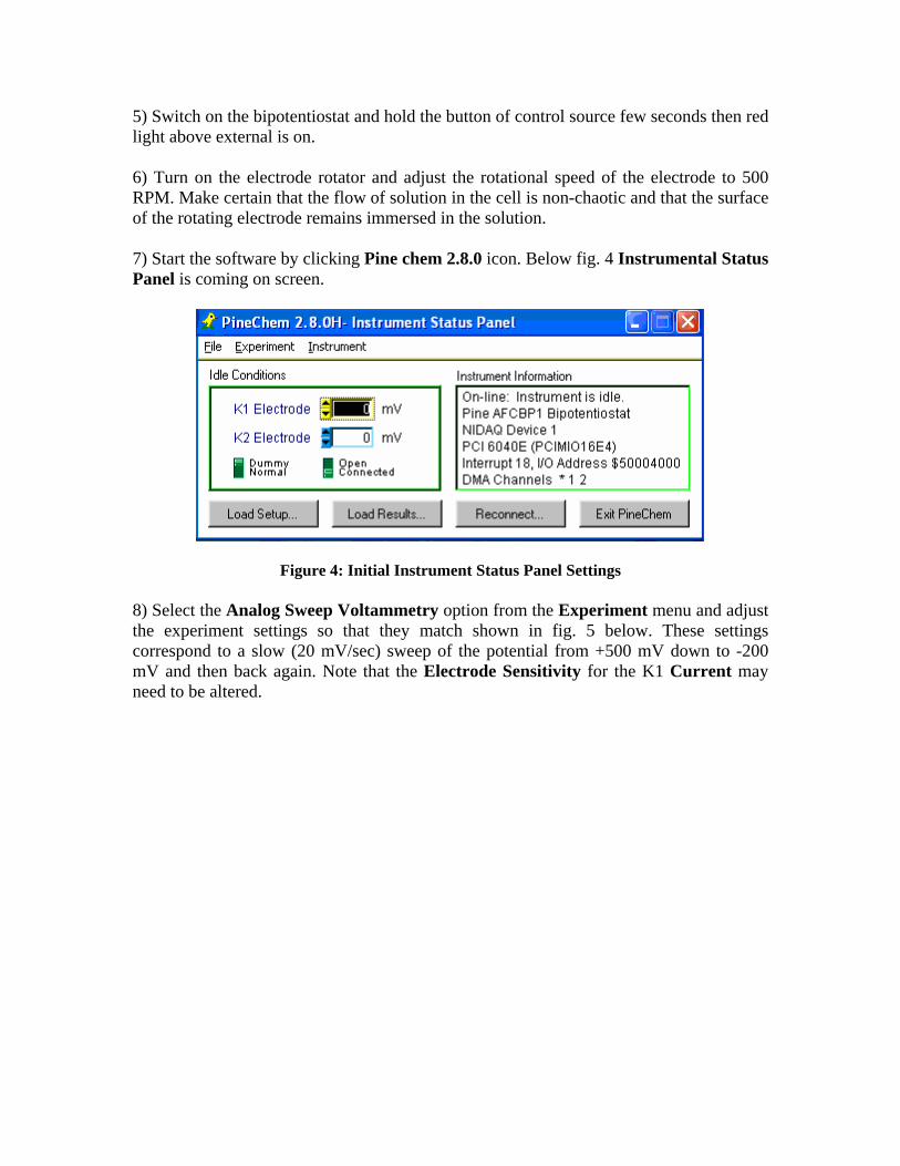
5) Switch on the bipotentiostat and hold the button of control source few seconds then red light above external is on. 6) Turn on the electrode rotator and adjust the rotational speed of the electrode to 500 RPM. Make certain that the flow of solution in the cell is non-chaotic and that the surface of the rotating electrode remains immersed in the solution. 7) Start the software by clicking Pine chem 2.8.0 icon. Below fig. 4 Instrumental Status Panel is coming on screen.
Figure 4: Initial Instrument Status Panel Settings 8) Select the Analog Sweep Voltammetry option from the Experiment menu and adjust the experiment settings so that they match shown in fig. 5 below. These settings correspond to a slow (20 mV/sec) sweep of the potential from +500 mV down to -200 mV and then back again. Note that the Electrode Sensitivity for the K1 Current may need to be altered.
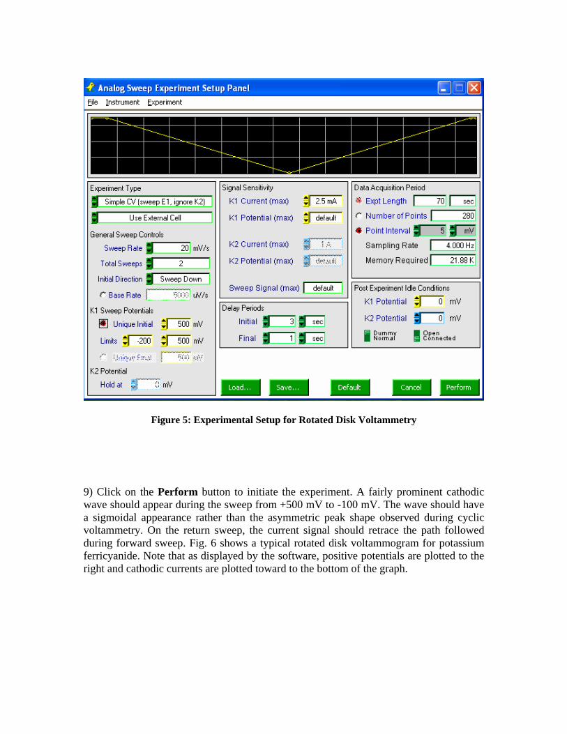
Figure 5: Experimental Setup for Rotated Disk Voltammetry
9) Click on the Perform button to initiate the experiment. A fairly prominent cathodic wave should appear during the sweep from +500 mV to -100 mV. The wave should have a sigmoidal appearance rather than the asymmetric peak shape observed during cyclic voltammetry. On the return sweep, the current signal should retrace the path followed during forward sweep. Fig. 6 shows a typical rotated disk voltammogram for potassium ferricyanide. Note that as displayed by the software, positive potentials are plotted to the right and cathodic currents are plotted toward to the bottom of the graph.
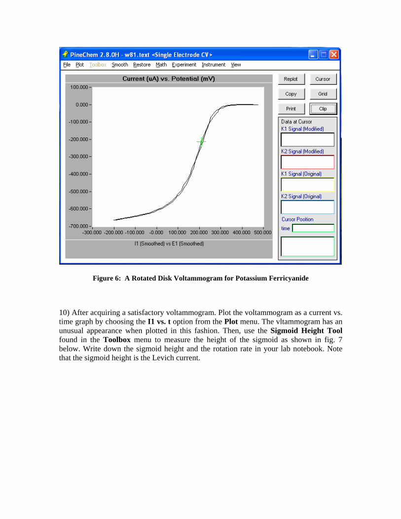
Figure 6: A Rotated Disk Voltammogram for Potassium Ferricyanide
10) After acquiring a satisfactory voltammogram. Plot the voltammogram as a current vs. time graph by choosing the I1 vs. t option from the Plot menu. The vltammogram has an unusual appearance when plotted in this fashion. Then, use the Sigmoid Height Tool found in the Toolbox menu to measure the height of the sigmoid as shown in fig. 7 below. Write down the sigmoid height and the rotation rate in your lab notebook. Note that the sigmoid height is the Levich current.
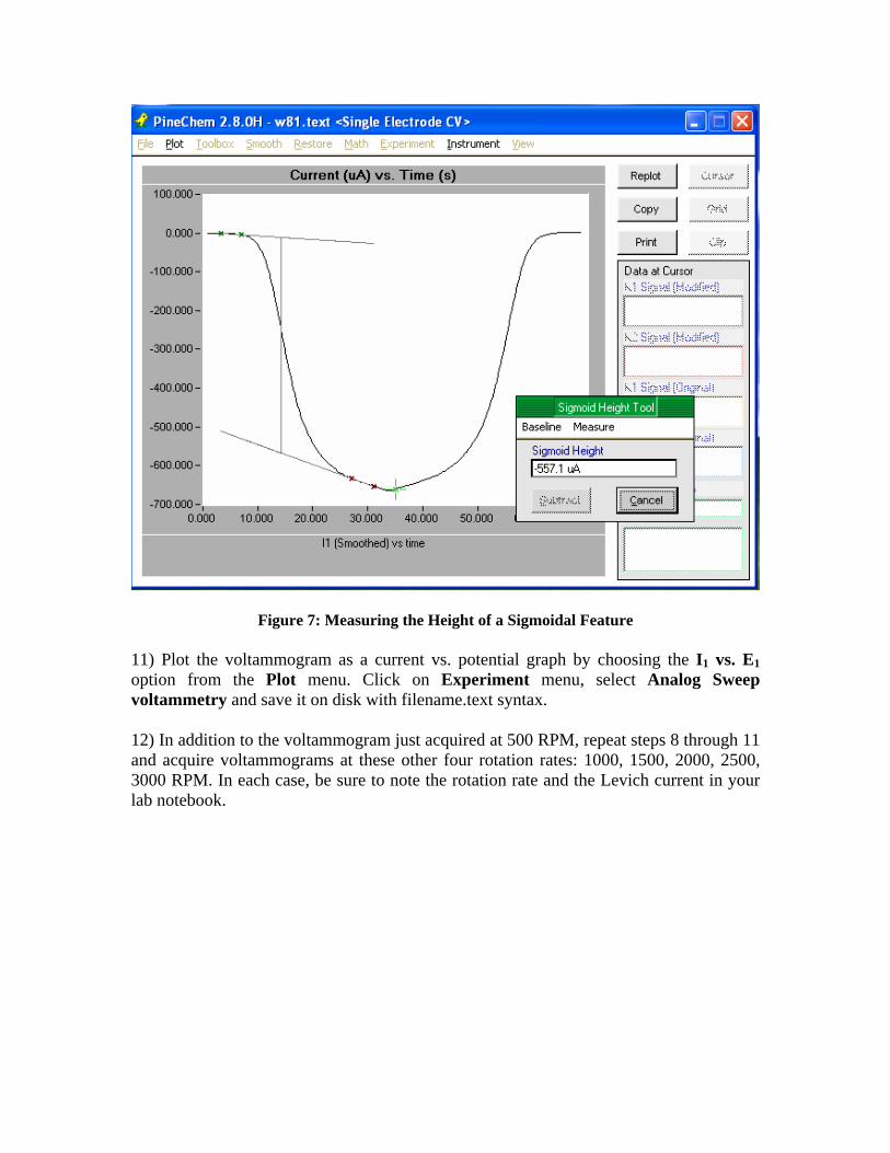
Figure 7: Measuring the Height of a Sigmoidal Feature 11) Plot the voltammogram as a current vs. potential graph by choosing the I1 vs. E1 option from the Plot menu. Click on Experiment menu, select Analog Sweep voltammetry and save it on disk with filename.text syntax. 12) In addition to the voltammogram just acquired at 500 RPM, repeat steps 8 through 11 and acquire voltammograms at these other four rotation rates: 1000, 1500, 2000, 2500, 3000 RPM. In each case, be sure to note the rotation rate and the Levich current in your lab notebook.
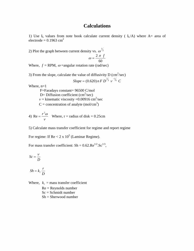
Calculations
1) Use IL values from note book calculate current density ( IL/A) where A= area of electrode = 0.1963 cm2
2) Plot the graph between current density vs. 21
ω
602 fπω =
Where, = RPM, f ω =angular rotation rate (rad/sec) 3) From the slope, calculate the value of diffusivity D (cm2/sec)
CDFnSlope 61
32
)620.0(−
= ν Where, n=1 F=Faradays constant= 96500 C/mol D= Diffusion coefficient (cm2/sec) ν = kinematic viscosity =0.00916 cm2/sec C = concentration of analyte (mol/cm3)
4) νω2Re r
= Where, r = radius of disk = 0.25cm
5) Calculate mass transfer coefficient for regime and report regime For regime: If Re < 2 x 10⁵ (Laminar Regime). For mass transfer coefficient: Sh = 0.62.Re1/2.Sc1/3,
DSc ν
=
DrkSh l=
Where, = mass transfer coefficient lk Re = Reynolds number Sc = Schmidt number Sh = Sherwood number
CL 610 – Experimental Methods
Experiment No. 6:
Dynamic surface Tensiometry Room No.: 225 (Organic Processing Lab)
Lab Manual
Department of Chemical Engineering,
Indian Institute of Technology, Bombay
CL 610: Experimental Methods
Determination of Dynamic Surface Tension of a Surfactant
Using a Bubble Pressure Tensiometer
TA: Shital D. Bachchhav
AIM:
(1) To determine the dynamic surface tension of a given surfactant solution using the maximum bubble pressure technique and show the effect of bubble frequency on surface tension for different concentration (2) To calculate the rate constant for demicellization of the given surfactant solution
INSTRUMENTS: Bubble pressure tensiometer
CHEMICALS AND APPARATUS:
Distilled water, Ethyl alcohol, Sodium dodecyl sulphate (SDS), Volumetric flasks, Conical flasks, Beakers, Pipette
THEORY:
The method is based on the measurement of the maximum pressure in a bubble growing at the tip of a capillary immersed into the liquid under study. When a bubble grows at the tip of a capillary, the pressure inside the capillary is measured. Maximum pressure is reached when the bubble is hemispherical, after which it grows quickly, separates from the capillary and a new bubble is formed. The maximum pressure depends on the liquid surface tension. The bubbles are generated at different frequencies allowing to characterize the dependency of surface tension on time. Bubble pressure tensiometry is used to study various dynamic surface phenomena including industrial and biological applications. Many industrial processes, such as coating, printing and flotation, operate under dynamic conditions and therefore surface tension determined within short life spans provides often more relevant information than equilibrium state values. Dependency of the surface tension on the concentration: Concentration is one of the parameter which has a decisive influence on the surface tension. The equilibrium value of the

surface tension decreases as the number of surfactant molecules accumulating at the surface increases. It achieves its final value when the surface is completely occupied and offers no place for further molecules. If the concentration is further increased from this point then the surfactant molecules will accumulate within the solution and form aggregates, the so-called “micelles. The concentration at which this effect occurs is known as the “critical micelle formation concentration” (CMC). It is an important characteristic of surfactants. This means that methods for measuring the dynamic surface tensions should only be used above the CMC. In such a case the concentration only influences the chronological function of the surface tension and no longer has any influence on its static value. Variation of surface tension with the bubble frequency: For pure solvents the dynamic surface tension does not change with the bubble rate. In case of multi component solution, the surface tension increase with the increasing bubbling frequency. At higher frequency the surfactant molecule does not have adequate time to diffuse to and orient them at the gas/liquid interface. Hence the surface tension increases.
EXPERIMENTAL PROCEDURE:
(1) The instrument was calibrated by measuring the corresponding voltage of pure water, pure ethanol, and ethanol-water mixture. (2) 5 mM sodium dodecyl sulphate (SDS) solution was taken as test solution in a glass beaker. (3) The voltage of the solution was measured with a bubble pressure tensiometer at bubble frequencies in the range of 0.5-3 bubbles/s. (4) In order to ensure the reproducibility of the collected data, all the measurement were performed in triplicate. (5) Steps 2-4 were repeated with 12.5 mM SDS solution
Table1: Calibration for pure water, ethanol, and ethanol-water mixture
Sample Surface Tension (mN/m) Voltage (volts) Pure Water
Pure Ethanol 15% (w/w) ethanol in water 40% (w/w) ethanol in water
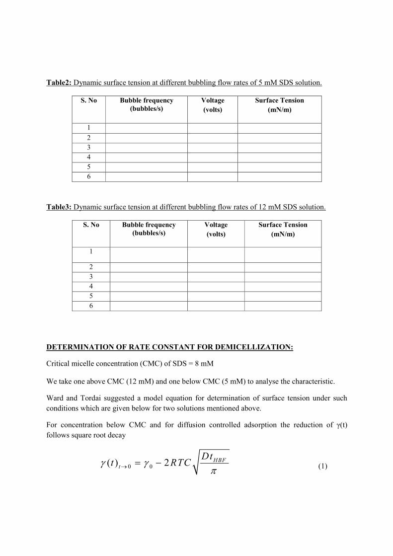
Table2: Dynamic surface tension at different bubbling flow rates of 5 mM SDS solution.
S. No Bubble frequency (bubbles/s)
Voltage
(volts)
Surface Tension
(mN/m)
1
2
3
4
5
6
Table3: Dynamic surface tension at different bubbling flow rates of 12 mM SDS solution.
S. No Bubble frequency (bubbles/s)
Voltage
(volts)
Surface Tension
(mN/m)
1
2
3
4
5
6
DETERMINATION OF RATE CONSTANT FOR DEMICELLIZATION:
Critical micelle concentration (CMC) of SDS = 8 mM We take one above CMC (12 mM) and one below CMC (5 mM) to analyse the characteristic.
Ward and Tordai suggested a model equation for determination of surface tension under such
conditions which are given below for two solutions mentioned above.
For concentration below CMC and for diffusion controlled adsorption the reduction of γ(t)
follows square root decay
0 0( ) 2 HBFt
Dtt RTC
(1)

For concentration above CMC and for diffusion controlled adsorption the reduction of γ(t)
follows square root decay
2
0
1( )
2
eq
t eq
L B F
R Tt
c t D k
(2)
Where, HBF and LBF are higher and lower bubble frequency respectively
γt→0 - Surface tension of the solution at highest bubble frequency
γ0 - Surface tension of pure water in N/m
R - Universal gas constant in J/mol K
T - Temperature of the solution in K
C- Bulk surfactant concentration in mol/m3
D - Diffusion coefficient in m2/s
t HBF- Surface age corresponding to highest bubble frequency in s
γt→∞ - Surface tension of the solution at lowest bubble frequency in N/m
γeq - Equilibrium surface tension in N/m
C0- Critical micelle concentration in mol/m3
Slope = d γeq/dlnc
Γeq = -1/RT (d γeq/dlnc) mol/m2

CL 610 – Experimental Methods
Experiment No. 6:
Dynamic surface Tensiometry Room No.: 225 (Organic Processing Lab)
Lab Manual
Department of Chemical Engineering,
Indian Institute of Technology, Bombay

CL 610: Experimental Methods
Determination of Dynamic Surface Tension of a Surfactant
Using a Bubble Pressure Tensiometer
TA: Shital D. Bachchhav
AIM:
(1) To determine the dynamic surface tension of a given surfactant solution using the maximum bubble pressure technique and show the effect of bubble frequency on surface tension for different concentration (2) To calculate the rate constant for demicellization of the given surfactant solution
INSTRUMENTS: Bubble pressure tensiometer
CHEMICALS AND APPARATUS:
Distilled water, Ethyl alcohol, Sodium dodecyl sulphate (SDS), Volumetric flasks, Conical flasks, Beakers, Pipette
THEORY:
The method is based on the measurement of the maximum pressure in a bubble growing at the tip of a capillary immersed into the liquid under study. When a bubble grows at the tip of a capillary, the pressure inside the capillary is measured. Maximum pressure is reached when the bubble is hemispherical, after which it grows quickly, separates from the capillary and a new bubble is formed. The maximum pressure depends on the liquid surface tension. The bubbles are generated at different frequencies allowing to characterize the dependency of surface tension on time. Bubble pressure tensiometry is used to study various dynamic surface phenomena including industrial and biological applications. Many industrial processes, such as coating, printing and flotation, operate under dynamic conditions and therefore surface tension determined within short life spans provides often more relevant information than equilibrium state values. Dependency of the surface tension on the concentration: Concentration is one of the parameter which has a decisive influence on the surface tension. The equilibrium value of the
surface tension decreases as the number of surfactant molecules accumulating at the surface increases. It achieves its final value when the surface is completely occupied and offers no place for further molecules. If the concentration is further increased from this point then the surfactant molecules will accumulate within the solution and form aggregates, the so-called “micelles. The concentration at which this effect occurs is known as the “critical micelle formation concentration” (CMC). It is an important characteristic of surfactants. This means that methods for measuring the dynamic surface tensions should only be used above the CMC. In such a case the concentration only influences the chronological function of the surface tension and no longer has any influence on its static value. Variation of surface tension with the bubble frequency: For pure solvents the dynamic surface tension does not change with the bubble rate. In case of multi component solution, the surface tension increase with the increasing bubbling frequency. At higher frequency the surfactant molecule does not have adequate time to diffuse to and orient them at the gas/liquid interface. Hence the surface tension increases.
EXPERIMENTAL PROCEDURE:
(1) The instrument was calibrated by measuring the corresponding voltage of pure water, pure ethanol, and ethanol-water mixture. (2) 5 mM sodium dodecyl sulphate (SDS) solution was taken as test solution in a glass beaker. (3) The voltage of the solution was measured with a bubble pressure tensiometer at bubble frequencies in the range of 0.5-3 bubbles/s. (4) In order to ensure the reproducibility of the collected data, all the measurement were performed in triplicate. (5) Steps 2-4 were repeated with 12.5 mM SDS solution
Table1: Calibration for pure water, ethanol, and ethanol-water mixture
Sample Surface Tension (mN/m) Voltage (volts) Pure Water
Pure Ethanol 15% (w/w) ethanol in water 40% (w/w) ethanol in water

Table2: Dynamic surface tension at different bubbling flow rates of 5 mM SDS solution.
S. No Bubble frequency (bubbles/s)
Voltage
(volts)
Surface Tension
(mN/m)
1
2
3
4
5
6
Table3: Dynamic surface tension at different bubbling flow rates of 12 mM SDS solution.
S. No Bubble frequency (bubbles/s)
Voltage
(volts)
Surface Tension
(mN/m)
1
2
3
4
5
6
DETERMINATION OF RATE CONSTANT FOR DEMICELLIZATION:
Critical micelle concentration (CMC) of SDS = 8 mM We take one above CMC (12 mM) and one below CMC (5 mM) to analyse the characteristic.
Ward and Tordai suggested a model equation for determination of surface tension under such
conditions which are given below for two solutions mentioned above.
For concentration below CMC and for diffusion controlled adsorption the reduction of γ(t)
follows square root decay
0 0( ) 2 HBFt
Dtt RTC
(1)

For concentration above CMC and for diffusion controlled adsorption the reduction of γ(t)
follows square root decay
2
0
1( )
2
eq
t eq
L B F
R Tt
c t D k
(2)
Where, HBF and LBF are higher and lower bubble frequency respectively
γt→0 - Surface tension of the solution at highest bubble frequency
γ0 - Surface tension of pure water in N/m
R - Universal gas constant in J/mol K
T - Temperature of the solution in K
C- Bulk surfactant concentration in mol/m3
D - Diffusion coefficient in m2/s
t HBF- Surface age corresponding to highest bubble frequency in s
γt→∞ - Surface tension of the solution at lowest bubble frequency in N/m
γeq - Equilibrium surface tension in N/m
C0- Critical micelle concentration in mol/m3
Slope = d γeq/dlnc
Γeq = -1/RT (d γeq/dlnc) mol/m2
CL 610 – Experimental Methods
Experiment No. 7: Stopped Flow Reactor
Room No.: 225 (Organic Processing Lab)
Lab Manual
Department of Chemical Engineering,
Indian Institute of Technology, Bombay
1. Aim:
To study the kinetics of a fast reactiondichlorophenolindophenol (DCPIP) by Ascorbic acid(AA)
2. Introduction:
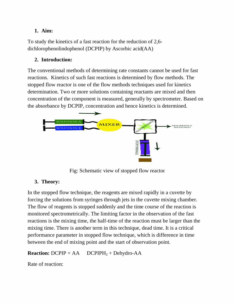
The conventional methods of determining rate constants cannot be used for fast reactions. Kinetics of such fast reactions is determined by flow methods. The stopped flow reactor is one of the flow methods techniques used for kinetics determination. Two or more solutions containing reactants are mixed and then concentration of the component is measured, generally by spectrometer. Based on the absorbance by DCPIP, concentration and hence kinetics is determined.
Fig: Schematic view of stopped flow reactor
3. Theory:
In the stopped flow technique, the reagents are mixed rapidly in a cuvette by forcing the solutions from syringes through jets in the cuvette mixing chamber. The flow of reagents is stopped suddenly and the time course of the reaction is monitored spectrometrically. The limiting factor in the observation of the fast reactions is the mixing time, the halfmixing time. There is another term in this technique, dead time. It is a critical performance parameter in stopped flow technique, which is difference in time between the end of mixing point and the start of observation point.
Reaction: DCPIP + AA DCPIPH
Rate of reaction:
kinetics of a fast reaction for the reduction of 2,6-dichlorophenolindophenol (DCPIP) by Ascorbic acid(AA)
The conventional methods of determining rate constants cannot be used for fast reactions. Kinetics of such fast reactions is determined by flow methods. The stopped flow reactor is one of the flow methods techniques used for kinetics
more solutions containing reactants are mixed and then concentration of the component is measured, generally by spectrometer. Based on the absorbance by DCPIP, concentration and hence kinetics is determined.
Fig: Schematic view of stopped flow reactor
In the stopped flow technique, the reagents are mixed rapidly in a cuvette by forcing the solutions from syringes through jets in the cuvette mixing chamber. The flow of reagents is stopped suddenly and the time course of the reaction is
spectrometrically. The limiting factor in the observation of the fast reactions is the mixing time, the half-time of the reaction must be larger than the mixing time. There is another term in this technique, dead time. It is a critical
er in stopped flow technique, which is difference in time between the end of mixing point and the start of observation point.
DCPIPH2 + Dehydro-AA
The conventional methods of determining rate constants cannot be used for fast reactions. Kinetics of such fast reactions is determined by flow methods. The stopped flow reactor is one of the flow methods techniques used for kinetics
more solutions containing reactants are mixed and then concentration of the component is measured, generally by spectrometer. Based on the absorbance by DCPIP, concentration and hence kinetics is determined.
In the stopped flow technique, the reagents are mixed rapidly in a cuvette by forcing the solutions from syringes through jets in the cuvette mixing chamber. The flow of reagents is stopped suddenly and the time course of the reaction is
spectrometrically. The limiting factor in the observation of the fast time of the reaction must be larger than the
mixing time. There is another term in this technique, dead time. It is a critical er in stopped flow technique, which is difference in time
]][[2 BAA CCk
dt
dC
Here, CA-concentration of DCPIP, CB-concentration of AA, k2-rate constant of the reaction. Defining M=CBO/CAO, the rate law after integration can be written in following form,
MtkCCC
CAOBO
A
B lnln 2
Hence the slope of
A
B
C
Cln vs time gives the rate constant.
If cocncentration of one of the reactants is in excess, then the reaction can be considered to be pseudo first order, hence rate law becomes,
][ AeffA Ck
dt
dC
Here keff = k1*[CB], effective pseudo first order rate constant and k1 is second order rate constant based on keff
After integration,
tkC
Ceff
A
AO
ln
4. Materials/ Instruments:
Chemicals:
De-ionized water, ascorbic acid, DCPIP
Apparautus:
MOS-200/M, FC-15 cuvette, SFM-20 equipped with 10ml syringes, Bio-Kine software, beakers volumetric flask.
5. Procedure: Prepare stock solutions of AA and DCPIP
Take absorption readings for water
Make calibration for DCPIP-water system
Record absorbance values for DCPIP-AA system at different mixing ratios
Rinse the system with DI water
6. Applications: protein folding, enzyme reactions, redox reactions.
7. Precautions: Air bubbles should not be present in the syringe.
One of the reactants must have absorption capacity.
8. References:1. Chemical reaction engineering (2nd edition), O.Levenspeil2. Prigodich R.V. A Stopped-Flow Kinetics Experiment for the Physical
ChemistryLaboratory Using Noncorrosive Reagents. J.Chem. Educ. 2014, 91, 2200-2202.
9. Questions :i. The half life of the reaction should be greater than the dead time. If the half-
life is shorter than the dead time, what will be the effect on the results?ii. What is advantage of stopped flow method than the continuous flow method
to study kinetics?iii. Can this method be useful to study the kinetics of slow rate reactions?iv. Reversible and irreversible reactions, which type of reactions, can be studied
by this method?v. Why the initial detectable concentration of the reactant is not equal to the
feed concentration of the reactant?
CL 610 – Experimental Methods
Experiment No. 8: Image Analysis
Lab Name: Fluid Mechanics Lab
Lab Manual
Department of Chemical Engineering,
Indian Institute of Technology, Bombay
Objective
To estimate Boltzmann constant, (kb) performing image analysis of Brownian motion of parti-cle.
Introduction
Although Jan Ingenhousz is known for the first person to make a documented observation offluctuating motion of carbon dust in alcohol in 1765, the discovery of Brownian motion iscredited to Robert Brown for his in depth observations of pollen in water in 1827. Brownianmotion is stochastic movement of small particles, (size ∼ 1µ) suspended in a solution. Solventmolecules hit the immersed particle, and the resulting force of the infinite number of collisionresults in a chaotic motion. The measurement of this motion can be done by the mean squaredisplacement, 〈(∆r)2〉 and the lag time ∆t. This motion is also characterized by the diffusioncoefficient, D which is the measure of the speed of diffusion.
Einstein published a paper in 1905 reporting the relationship between the mean square mag-nitude of displacement due to Brownian motion and the size of particles. French Physicist JeanBaptiste Perrin’s experimental evidence justified Einstein’s hypothesis and thereby confirmedthe atomic nature of the matter. For this study he has been awarded Nobel prize for Physicsin 1926. Since then, a thorough understanding of Brownian motion has find its importance notonly in polymer physics to biophysics, aerodynamics to statistical mechanics but also in stockoption pricing.
Boltzmann constant can be calculated from various experimental methods few of whichinclude
• Image analysis
• Acoustic gas thermometry
• Quasi-spherical cavity resonators
• Dielectric constant gas thermometry
• Doppler broadening thermometry
• Noise thermometry.
In this experiment, we will follow the Image Analysis technique to calculate the value of Boltz-mann constant, kb.
1
Theoretical and mathematical background
Kinetic theory suggests that any particle has the same average translational kinetic energy irre-spective to their size. In 3 dimension the value of this average translational energy is 3
2kbT i.e.
12kbT for each degrees of freedom, where T is the absolute temperature in Kelvin scale. The
velocity of particle is directly proportional to square root of T and inversely proportional tosquare root of mass. Einstein has calculated the diffusion coefficient for a spherical Brownianparticle as
D =kbT
6πηa, (1)
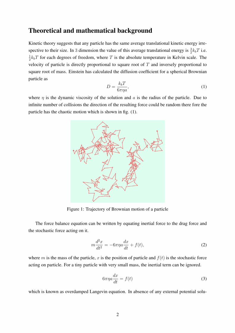
where η is the dynamic viscosity of the solution and a is the radius of the particle. Due toinfinite number of collisions the direction of the resulting force could be random there fore theparticle has the chaotic motion which is shown in fig. (1).
Figure 1: Trajectory of Brownian motion of a particle
The force balance equation can be written by equating inertial force to the drag force andthe stochastic force acting on it.
md2x
dt2= −6πηa
dx
dt+ f(t), (2)
where m is the mass of the particle, x is the position of particle and f(t) is the stochastic forceacting on particle. For a tiny particle with very small mass, the inertial term can be ignored.
6πηadx
dt= f(t) (3)
which is known as overdamped Langevin equation. In absence of any external potential solu-
2
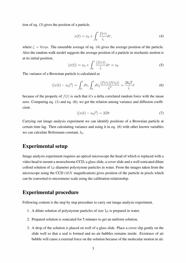
tion of eq. (3) gives the position of a particle.
x(t) = x0 +
∫ t
0
f(τ)
ζdτ, (4)
where ζ = 6πηa. The ensemble average of eq. (4) gives the average position of the particle.Also the random walk model suggests the average position of a particle in stochastic motion isat its initial position.
〈x(t)〉 = x0 +
∫ t
0
〈f(τ)〉ζ
dτ = x0 (5)
The variance of a Brownian particle is calculated as
〈(x(t)− x0)2〉 =
∫ t
0
dτ1
∫ t
0
dτ2〈f(τ1)f(τ2)〉
ζ2=
2kbT
ζt (6)
because of the property of f(t) is such that it’s a delta correlated random force with the meanzero. Comparing eq. (1) and eq. (6), we get the relation among variance and diffusion coeffi-cient.
〈(x(t)− x0)2〉 = 2Dt (7)
Carrying out image analysis experiment we can identify positions of a Brownian particle atcertain time lag. Then calculating variance and using it in eq. (6) with other known variableswe can calculate Boltzmann constant, kb.
Experimental setup
Image analysis experiment requires an optical microscope the head of which is replaced with avideo head to mount a monochrome CCD, a glass slide, a cover slide and a well sonicated dilutecolloid solution of 1µ diameter polystyrene particles in water. From the images taken from themicroscope using the CCD (40X magnification) gives position of the particle in pixels whichcan be converted to micrometer scale using the calibration relationship.
Experimental procedure
Following content is the step by step procedure to carry out image analysis experiment.
1. A dilute solution of polystyrene particles of size 1µ is prepared in water.
2. Prepared solution is sonicated for 5 minutes to get an uniform solution.
3. A drop of the solution is placed on well of a glass slide. Place a cover slip gently on theslide well so that a seal is formed and no air bubbles remains inside. Existence of airbubble will cause a external force on the solution because of the molecular motion in air.
3
4. The slide is placed under microscope for observation. Illumination of the microscopeand the focus is adjusted to obtain the best image.
5. Twenty snapshots of the well focused particles in solution are captured at a certain lagtime, ∆t using IMAGE PRO software interface installed in the PC attached with thecamera.
6. Position of a particle, (values in x and y co-ordinates) at different snapshots are mea-sured using image processing software interface IMAGE J and stored in a file for furthercalculations.
7. Measured co-ordinates are converted to µ from pixels using standard calibration data.
8. Above procedure is followed for 8 different values of time lag, ∆t.
9. Room temperature is noted down.
Observations and calculations
Measured variables data
• Temperature:
• Dynamic viscosity of water:
• Radius of polystyrene particles:
4
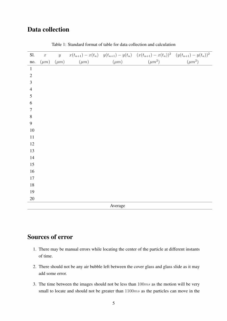
Data collection
Table 1: Standard format of table for data collection and calculation
Sl. x y x(tn+1)− x(tn) y(tn+1)− y(tn) (x(tn+1)− x(tn))2 (y(tn+1)− y(tn))2
no. (µm) (µm) (µm) (µm) (µm2) (µm2)
1234567891011121314151617181920
Average
Sources of error
1. There may be manual errors while locating the center of the particle at different instantsof time.
2. There should not be any air bubble left between the cover glass and glass slide as it mayadd some error.
3. The time between the images should not be less than 100ms as the motion will be verysmall to locate and should not be greater than 1100ms as the particles can move in the
5

z-direction and thus, exact displacement can not be recognized.
4. Care should be taken on tracing only one single particle. If for one set of data 2 particlesare being traced then error will be huge.
5. Particle with minimal diffusion in z direction during the time of reference should betaken.
6
Experiment No. 9: Vapour Pressure
Osmometer
Room No.: 227 (Organic Processing lab)
Lab Manual
Department of Chemical Engineering,
Indian Institute of Technology, Bombay
Objective Vapour Pressure Osmometry
Determination of molecular weight of given salt using vapour pressure osmotry.
Introduction
Salt is very essential for the sustenance of the human body which can endure for long periods
without food but without water and salt, the living cells would die from dehydration and other than that it has its applications in the food industry as preservative being a very safe and
inexpensive desiccant. Similar kind of compounds need to be used for calibration and molecular weight determination . Otherwise there could be considerable deviation in the actual and
experimental values to the way they differ in their interaction with the solvent (water in our case). Therefore, NaCl has been used for calibration to find out the molecular weight of the salt
KCl.
THEORY
Determination of number average molecular weight depends on basic equations of dilute
solution chemistry and physical chemistry. In a dilute solution, the vapour pressure of a
solvent is given by basic Raoult’s Law:
P1=P10 *X1
P1 = partial pressure of solvent in solution
P10 = vapor pressure of pure solvent
X1 = mole fraction of solvent
So, vapour pressure of any solution is lower than vapour pressure of its pure solvent. If one
places the drop of solution along with that of pure solvent in the vapour environment of pure
solvent, then condensation will occur on the solution drop because its vapour pressure will be
less than that of the solvent. Condensation will lead to relative increase in temperature of the
solution drop with respect to the pure solvent drop. Increased temperature in turn changes
resistance and hence, generates a potential difference. This potential difference is recorded
until equilibrium is reached.
The basic relation for molecular mass determination equals:
msample
nsample =
M sample
msolvent msolvent
n = Number of sample molecules
M ( g
m = Mass of sample and solvent respectively M = Molecular mass of the sample
For a molecular mass less than 500 g/mol the measurement value is proportional to the
number of moles. The change in vapour pressure is proportional to the number of species
present in the solution, which is measured in terms of osmol units. Hence the this is very
similar to the osmolality determination. A sample is measured where concentration and
molecular mass are known (c in mol/kg). The slope of the graph of measurement value v/s
concentration is calib with kg/mol.
K calibration = MV
c
Unknown molecular mass of the sample can be determined by a known concentration. The
slope of the curve of measured value gives Kmeasurement
The molecular weight of unknown sample is determined with:
mol )= Kcalibration / Kmeasurement
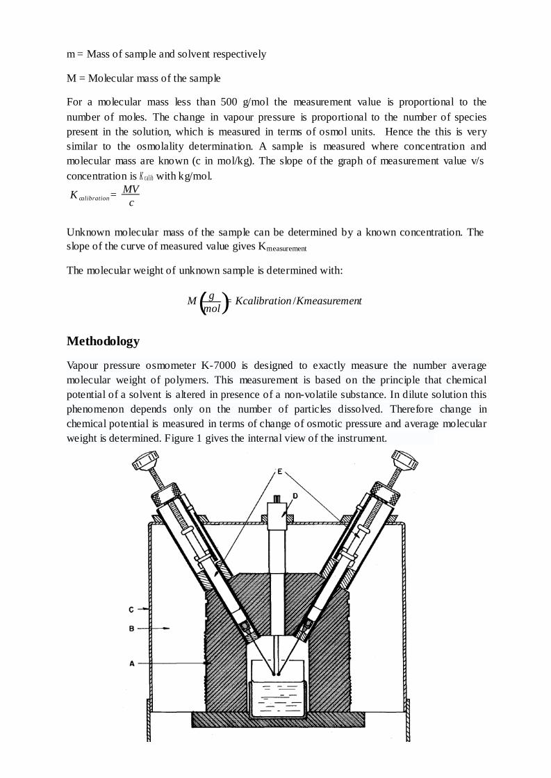
Methodology
Vapour pressure osmometer K-7000 is designed to exactly measure the number average
molecular weight of polymers. This measurement is based on the principle that chemical
potential of a solvent is altered in presence of a non-volatile substance. In dilute solution this
phenomenon depends only on the number of particles dissolved. Therefore change in
chemical potential is measured in terms of change of osmotic pressure and average molecular
weight is determined. Figure 1 gives the internal view of the instrument.
Apparatus Vapour pressure osmometer, volumetric flasks, pipette
Chemicals NaCl (AR Grade), Millipore water, KCl
PROCEDURE
1. Prepare samples of different concentration for which molecular weight is to be
determined
2. Check whether thermistors are working or not
Press TEST, if it displays OK then carry on, otherwise stop.
3. Fill 25% of beaker with pure solvent along with the wick.
4. Insert the thermistor assembly inside the beaker and place it in an equipment chamber
and tighten to avoid leakage which will disturb the stabilization.
5. Place all the syringes inside the syringe ports. Fill two syringes with pure solvent and
place them back to the syringe holders to attain the temperature of head.
6. Set the temperature according to your requirement but within a limit given in an
equipment manual for different solvents. Selectable cell temperature 20OC -130OC.
7. After temperature setting, place GAIN value to maximum (256).Then let it stabilize.
Selectable gain settings are 1,2,4,8,16,32,64,128,256
8. Before starting the experiment adjust the Wheatstone bridge signal value to zero with the
help of AUTOZERO function. After that add a drop of one of the solution prepared on
one thermistor. If the signal value is showing OVERLOAD then adjust the gain
accordingly to get signal value. In this way note down the signal and gain value for every
solution.
RESULTS
Table1: Calibration data for standard solute (NaCl)
Concentration of NaCl (mole/lt)
Gain
Signal (mv)
Signal/Gain
Average Signal (mv)
0.3 16
8
0.4 8
4
0.5 8
4
0.6
4
2
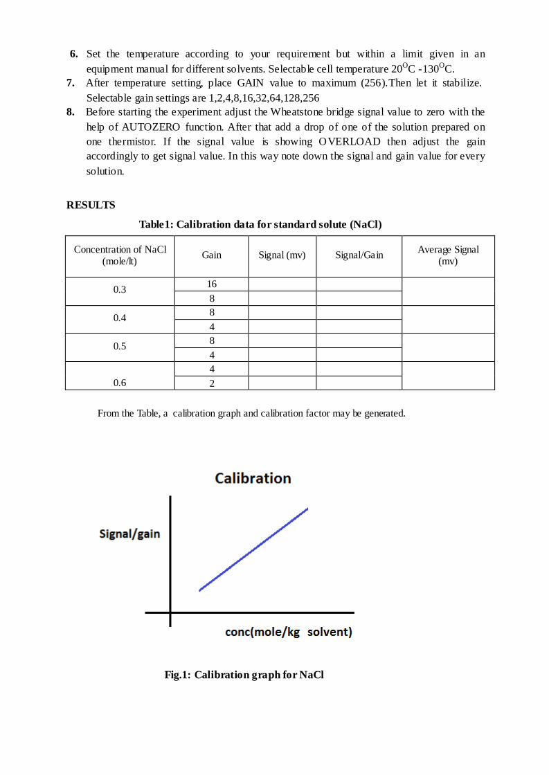
From the Table, a calibration graph and calibration factor may be generated.
Fig.1: Calibration graph for NaCl
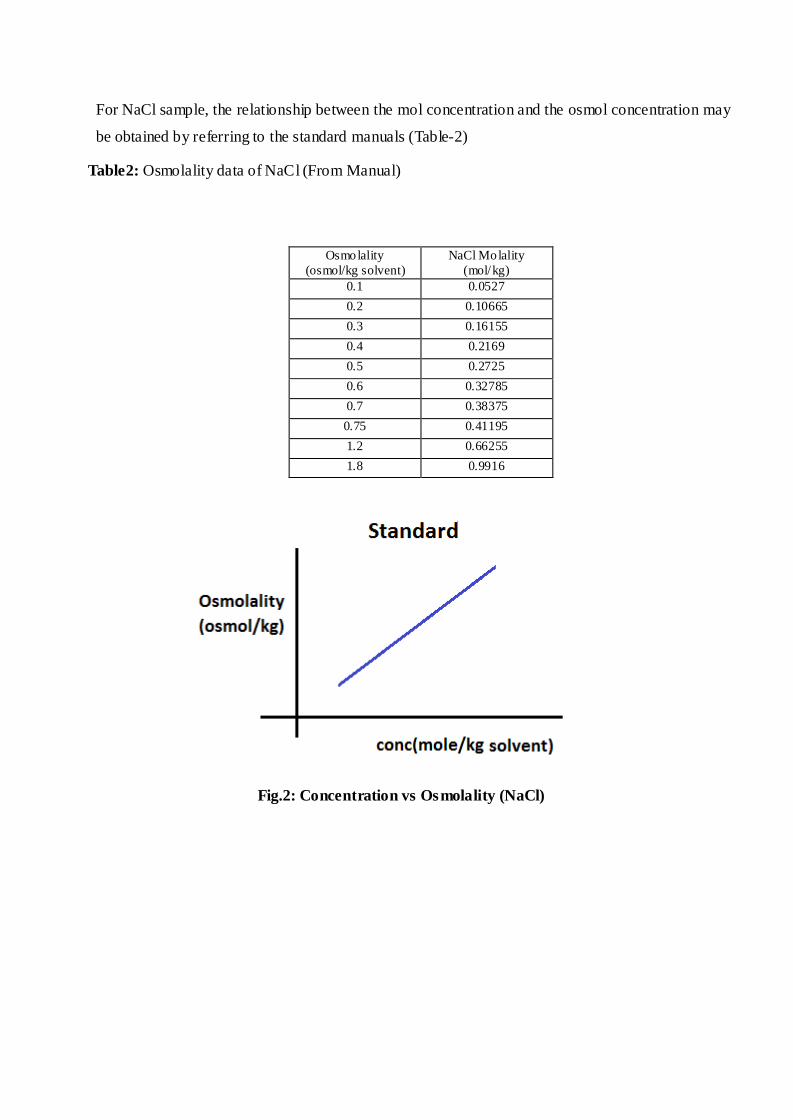
For NaCl sample, the relationship between the mol concentration and the osmol concentration may
be obtained by referring to the standard manuals (Table-2)
Table2: Osmolality data of NaCl (From Manual)
Fig.2: Concentration vs Osmolality (NaCl)
Osmolality
(osmol/kg solvent)
NaCl Molality
(mol/kg)
0.1 0.0527
0.2 0.10665
0.3 0.16155
0.4 0.2169
0.5 0.2725
0.6 0.32785
0.7 0.38375
0.75 0.41195
1.2 0.66255
1.8 0.9916
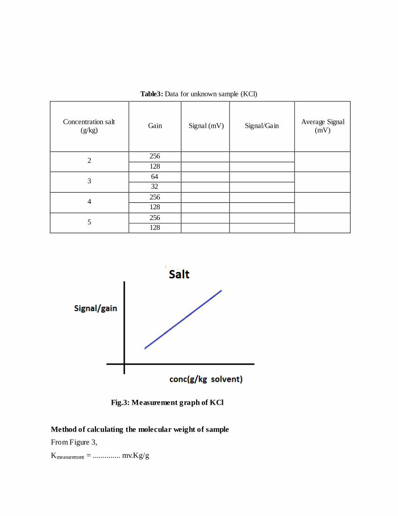
Table3: Data for unknown sample (KCl)
Concentration salt (g/kg)
Gain
Signal (mV)
Signal/Gain
Average Signal (mV)
2 256
128
3 64
32
4 256
128
5 256
128
Fig.3: Measurement graph of KCl
Method of calculating the molecular weight of sample
From Figure 3,
Kmeasurement = .............. mv.Kg/g
Molecular weight of KCl = Kcalibration/ Kmeasurement = ..............g/Osmol.
This weight is then converted into molar weight depending on the interaction of KCl with
water .
Discussions and Conclusion
The reasons for deviation of experimental form actual (if any) should be analyzed and reasons
may be given( improper contact between thermistor tip and drop, drop size etc.)
Reading material
Vapor pressure osmometry as a means of determining polymer molecular weight, I.J Goldfab, A.C. Meeks, May 1996
CL 610 – Experimental Methods
Lab Manual
Nanoparticle Aerosol Size
Distribution
Room No.: 321 (Particle and Aerosol
Research Lab)
Department of Chemical Engineering,
Indian Institute of Technology, Bombay
CL610-Experimental Methods
Experiment No.10
Nanoparticle aerosol size distribution measurement using a Scanning Mobility Particle Sizer
(SMPS)
TAs:
Suraj Ugrani
Lab Location:
Particle and Aerosol Research Laboratory (PeARL), Room 321, 2nd
Floor
Department of Chemical Engineering
Indian Institute of Technology-Bombay
Spring, 2016
1. Objectives - Understand the principle of aerosol measurement using a Scanning Mobility Particle
Sizer (SMPS).
- Carry out aerosol synthesis of stearic acid nanoparticles with controlled median
diameter.
- Derive the power law exponent relating median nanoparticle size to precursor
concentration.
- Fit log-normal size distributions and derive size distribution parameters.
2. Introduction An aerosol is a metastable, gaseous suspension of multiphase particles. Aerosol
measurement is a complex and elegant field of research, wherein instruments have been
developed based, both on laser light scattering or particle charging followed by mobility
measurements along with optical detection, to size particles of 2.5 nm to 20 µm diameter and
count number concentrations (ranging from 102-10
5 particles/cm
3) quantitatively.
Aerosol routes to process materials into nanoparticles rely on high temperature
nucleation-coagulation processes or controlled temperature droplet drying of solution
aerosols (gas-phase suspensions of liquid or solid particles) in aerosol flow reactors. Unlike
colloidal methods of nanoparticles synthesis, which utilize several post-processing separation
steps, aerosol methods offer a single-step continuous method for producing nanoparticles
which can be collected as dry powders or directly into liquid media to form a suspension. The
aerosol route has been used to prepare nanoparticles for catalyst, photoelectric, drug delivery.
In this experiment, the aerosol route will be used to make stearic acid nanoparticles of
controlled median diameter. The principle of aerosol measurement using mobility sizing will
be demonstrated, to measure and analyse nanoparticle size distribution.
3. Theory When a charged nanoparticle is exposed to an electric field, it migrates at a velocity
that is determined by a balance between the resulting electrostatic force and aerodynamic
drag that resists its motion. This characteristic migration velocity is described as electrical
mobility of the particle, 𝑍, the migration velocity per unit of applied electrical field strength.
3.1. Non-continuum effects
The force resisting the motion of a sphere passing through a fluid is the drag force.
The Stokes‟ law form, 𝐹𝐷 = 3𝜋𝜇𝑉𝑑𝑝 , hold for a rigid sphere that moves through a fluid at
constant velocity, with particle Reynolds number much less than unity. The particle can be
many diameters away from surface and much larger than mean free path of the gas
molecules, 𝜆, which is about 0.0065𝜇𝑚 at 250C.
For small particles whose size approaches the mean free path of gas where (𝑑𝑝 ≈ 𝜆 ),
the drag for a given velocity becomes less than predicted from Stokes law and continues to
decrease with particle size. These particles experience a slip at the surface, termed non-
continuum effect. The „slip effect‟ is corrected by introducing Cunningham correction factor
(or slip correction factor) 𝐶𝑐 for particles less than 0.1 µm diameter (Allen and Raabe 1985),
which follow either “free molecular” or “intermediate” regime behaviour. An interpolation
formula below calculates the slip factor over both regimes of particle behaviour.
𝐹𝐷 =3𝜋𝜇𝑉𝑑𝑝
𝐶𝑐 Eqn. 1
𝐶𝑐 = 1 + 𝐾𝑛 1.142 + 0.558 exp −0.999
𝐾𝑛 Eqn. 2
Kn is Knudsen number = 2λ /dp
3.2. Bipolar diffusion charging
An effective method of charging nanoparticles to obtain unit charge (with a high
probability) bipolar diffusion charging. It has been hypothesized that, after long exposure to
such bipolar ion mixtures, frequent ion-particle collisions will bring the particles to a state of
charge equilibrium with the ionic atmosphere. In this equilibrium state, the fraction of
particles of diameter 𝑑𝑃 that carry 𝑖 charges is described by the Boltzmann charge
distribution, that is,
𝑃 𝑑𝑝 , 𝑖 =exp −
𝑖2
2𝜎2
exp −𝑘2
2𝜎2 ∞𝑘→−∞
Eqn. 3
𝜎2 =𝑑𝑝𝑘𝑇
2𝑒2 Eqn. 4
3.3. Particle mobility in an electric field
A particle with charge 𝑞 in an electric field of strength 𝐸 experiences a force of
strength 𝐹 = 𝑞𝐸. Because of the low ion densities and slow charge transfer kinetics in
ambient temperature gases, aerosol particles usually carry only a small number of elementary
charges. The charge is, therefore, conveniently represented as 𝑞 = 𝑖𝑒, where 𝑒 = 1.609 𝑥 10−19 is the magnitude of the elementary unit of (𝑖 < 0 for negatively charged
particles, and 𝑖 > 0 for positively charged particles). For times that are long compared with
the aerodynamic relaxation time, 𝜏𝑎 = 𝑚𝑝𝐵, (𝑚𝑝 is the particle mass and 𝐵 is electrical
mobility of the particle), a charged particle will migrate at a steady-state migration velocity
𝑣𝑒 relative to the gas motion 𝑢 of
𝑣𝑒 = 𝑣 − 𝑢 = 𝑖𝑒𝐵𝐸 = 𝑍𝐸 Eqn. 5
For motion of spherical particles with diameter 𝑑𝑝 in Stokes regime, this mobility is
𝑍 =𝑖𝑒𝐶𝑐
3𝜋𝜂𝑑𝑝= 𝑓(𝐾𝑛) Eqn. 6
𝐶𝑐 = slip correction factor, 𝐾𝑛 = Knudsen No. = 2𝜆/𝑑𝑝 , 𝜆= mean free path of gas molecules,
𝜂= gas viscosity.
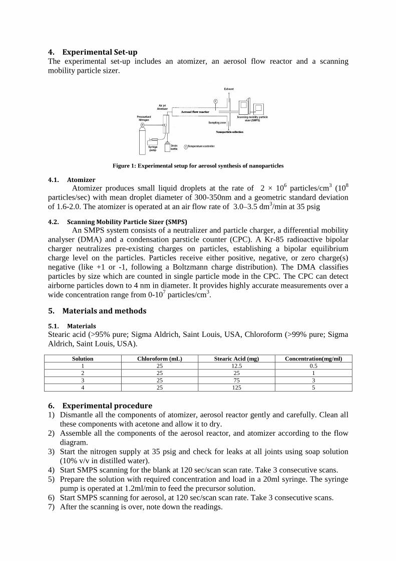
4. Experimental Set-up The experimental set-up includes an atomizer, an aerosol flow reactor and a scanning
mobility particle sizer.
Figure 1: Experimental setup for aerosol synthesis of nanoparticles
4.1. Atomizer
Atomizer produces small liquid droplets at the rate of 2 × 10⁶ particles/cm
3 (10
8
particles/sec) with mean droplet diameter of 300-350nm and a geometric standard deviation
of 1.6-2.0. The atomizer is operated at an air flow rate of 3.0–3.5 dm3/min at 35 psig
4.2. Scanning Mobility Particle Sizer (SMPS)
An SMPS system consists of a neutralizer and particle charger, a differential mobility
analyser (DMA) and a condensation parsticle counter (CPC). A Kr-85 radioactive bipolar
charger neutralizes pre-existing charges on particles, establishing a bipolar equilibrium
charge level on the particles. Particles receive either positive, negative, or zero charge(s)
negative (like +1 or -1, following a Boltzmann charge distribution). The DMA classifies
particles by size which are counted in single particle mode in the CPC. The CPC can detect
airborne particles down to 4 nm in diameter. It provides highly accurate measurements over a
wide concentration range from 0-107 particles/cm
3.
5. Materials and methods
5.1. Materials
Stearic acid (>95% pure; Sigma Aldrich, Saint Louis, USA, Chloroform (>99% pure; Sigma
Aldrich, Saint Louis, USA).
Solution Chloroform (mL) Stearic Acid (mg) Concentration(mg/ml)
1 25 12.5 0.5
2 25 25 1
3 25 75 3
4 25 125 5
6. Experimental procedure 1) Dismantle all the components of atomizer, aerosol reactor gently and carefully. Clean all
these components with acetone and allow it to dry.
2) Assemble all the components of the aerosol reactor, and atomizer according to the flow
diagram.
3) Start the nitrogen supply at 35 psig and check for leaks at all joints using soap solution
(10% v/v in distilled water).
4) Start SMPS scanning for the blank at 120 sec/scan scan rate. Take 3 consecutive scans.
5) Prepare the solution with required concentration and load in a 20ml syringe. The syringe
pump is operated at 1.2ml/min to feed the precursor solution.
6) Start SMPS scanning for aerosol, at 120 sec/scan scan rate. Take 3 consecutive scans.
7) After the scanning is over, note down the readings.
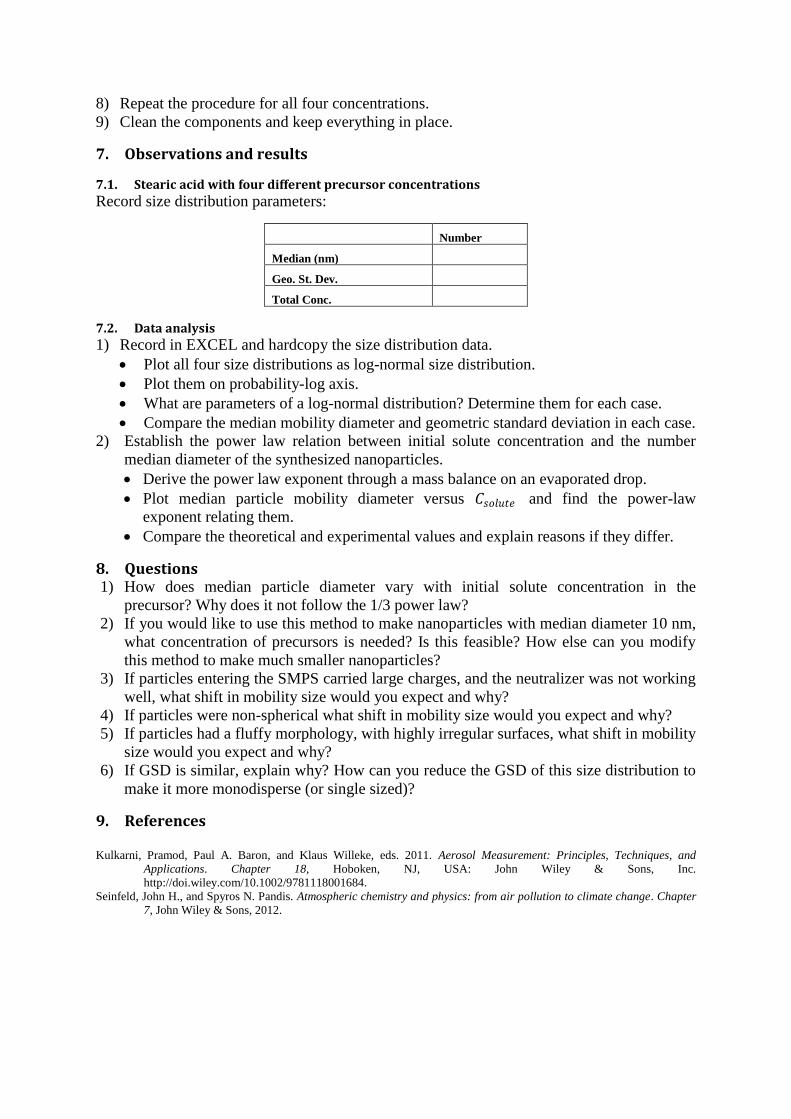
8) Repeat the procedure for all four concentrations.
9) Clean the components and keep everything in place.
7. Observations and results
7.1. Stearic acid with four different precursor concentrations
Record size distribution parameters:
Number
Median (nm)
Geo. St. Dev.
Total Conc.
7.2. Data analysis
1) Record in EXCEL and hardcopy the size distribution data.
Plot all four size distributions as log-normal size distribution.
Plot them on probability-log axis.
What are parameters of a log-normal distribution? Determine them for each case.
Compare the median mobility diameter and geometric standard deviation in each case.
2) Establish the power law relation between initial solute concentration and the number
median diameter of the synthesized nanoparticles.
Derive the power law exponent through a mass balance on an evaporated drop.
Plot median particle mobility diameter versus 𝐶𝑠𝑜𝑙𝑢𝑡𝑒 and find the power-law
exponent relating them.
Compare the theoretical and experimental values and explain reasons if they differ.
8. Questions 1) How does median particle diameter vary with initial solute concentration in the
precursor? Why does it not follow the 1/3 power law?
2) If you would like to use this method to make nanoparticles with median diameter 10 nm,
what concentration of precursors is needed? Is this feasible? How else can you modify
this method to make much smaller nanoparticles?
3) If particles entering the SMPS carried large charges, and the neutralizer was not working
well, what shift in mobility size would you expect and why?
4) If particles were non-spherical what shift in mobility size would you expect and why?
5) If particles had a fluffy morphology, with highly irregular surfaces, what shift in mobility
size would you expect and why?
6) If GSD is similar, explain why? How can you reduce the GSD of this size distribution to
make it more monodisperse (or single sized)?
9. References Kulkarni, Pramod, Paul A. Baron, and Klaus Willeke, eds. 2011. Aerosol Measurement: Principles, Techniques, and
Applications. Chapter 18, Hoboken, NJ, USA: John Wiley & Sons, Inc.
http://doi.wiley.com/10.1002/9781118001684.
Seinfeld, John H., and Spyros N. Pandis. Atmospheric chemistry and physics: from air pollution to climate change. Chapter
7, John Wiley & Sons, 2012.
CL:610-Experimental Methods Spring, 2016
Expt No.11
Atomic Absorption Spectroscopy
Determination of the concentration of metal ion using Atomic Absorption
Spectroscopy
Course Instructor:
Prof. Chandra V.
TA:Hridoy Mahanta
Department of Chemical Engineering
Indian Institute of Technology-Bombay
Objective:
To determine the concentration of metal ion using Atomic Absorption
Spectroscopy (AAS). Chemical Required:
Stock solutions of metal ions:Copper Sulphate and Ferrous Ammonium
Sulphate(FAS),Milipore water
Apparatus Required:
Glass wares
Instrument Used:
Atomic Absorption Spectrometer (Model: GBC-902)
Theory:
Atomic absorption spectroscopy is an analytical procedure used for
quantitative analysis of metals and some metalloids based on the absorption
of optical radiation (light) by free atoms in the gaseous state. AAS can be
used to determine over 70 di erent elements in solu-tion or directly in solid
samples. The concept of atomic absorption spectrometry (AAS) was
2
proposed by two groups in 1955, A. Walsh of Australia and another one of
C.T.J Alkamade and J.M.W Milatz from The Netherlands. It is basically the study of absorption spectra by means of passing electro-
magnetic radiation through an atomic medium that is selectively absorbing;
this produces pure electronic tran-sitions free from vibrational and rotational
transitions. In this method, the amount of light at the resonant wavelength
which is absorbed as it passes through a cloud of atoms is measured. As the
number of atoms in the light path increases, the amount of light absorbed
increases in a predictable way. By measuring the amount of light absorbed, a
quantitative determination of the amount of analyte element present can be
made. The use of special light sources and careful selection of wavelength
allow the specific quantitative determination of individual elements in the
presence of others.
The atom cloud required for atomic absorption measurements is produced
by supplying enough thermal energy to the sample to dissociate the chemical
compounds into free atoms. This is done by aspirating liquid samples into an
air-acetylene flame, causing evaporation of the solvent and vaporization of
the free metal atoms. A line source (hollow cathode lamp) is used to cause
electronic excitation of the metal atoms, and the absorbance is measured with
a conventional spectrometer with photomultiplier detector.
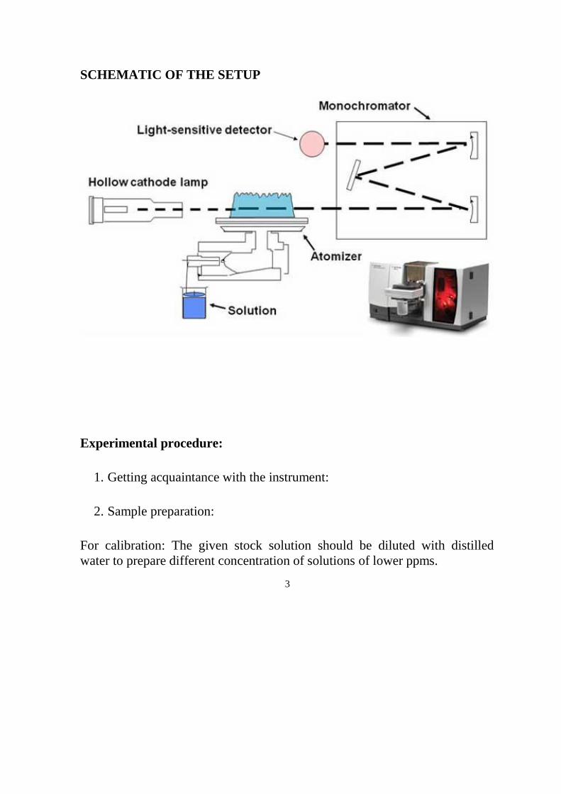
SCHEMATIC OF THE SETUP
Experimental procedure:
1. Getting acquaintance with the instrument:
2. Sample preparation: For calibration: The given stock solution should be diluted with distilled
water to prepare different concentration of solutions of lower ppms. 3

3. Setting up of instrument:
The exhaust and hood should be put on.
Set up the corresponding slit width and wavelength.
Select and fit the lamp corresponding for the given metal ion.
Put the mains of instrument on. Switch on the power switch Set up the
current for the lamp as given in instrument manual.
Get the maximum signal in the energy meter of the instrument.
Open air cylinder and adjust the flow rate. Similarly open acetylene cylinder and adjust the flow rate.
4
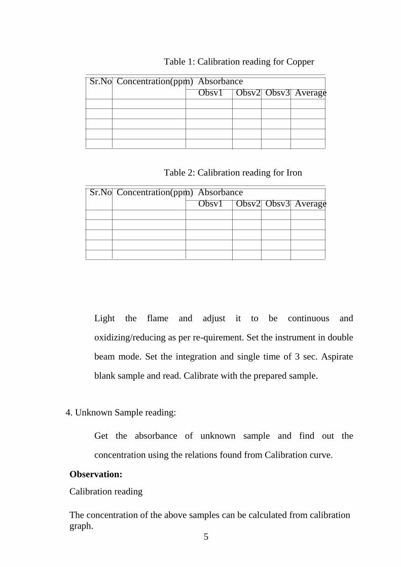
Table 1: Calibration reading for Copper
Sr.No Concentration(ppm) Absorbance
Obsv1 Obsv2 Obsv3 Average
Table 2: Calibration reading for Iron
Sr.No Concentration(ppm) Absorbance Obsv1 Obsv2 Obsv3 Average
Light the flame and adjust it to be continuous and
oxidizing/reducing as per re-quirement. Set the instrument in double
beam mode. Set the integration and single time of 3 sec. Aspirate
blank sample and read. Calibrate with the prepared sample.
4. Unknown Sample reading:
Get the absorbance of unknown sample and find out the
concentration using the relations found from Calibration curve.
Observation: Calibration reading
The concentration of the above samples can be calculated from calibration
graph.
5
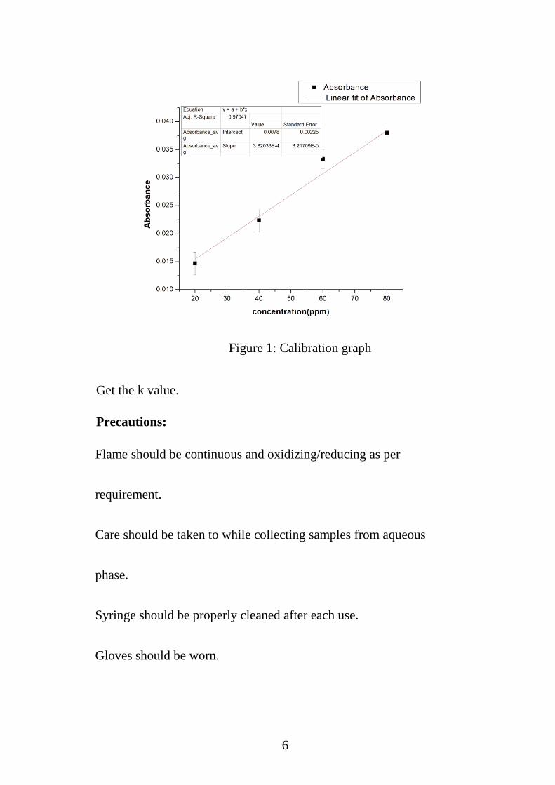
Figure 1: Calibration graph Get the k value.
Precautions:
Flame should be continuous and oxidizing/reducing as per
requirement.
Care should be taken to while collecting samples from aqueous
phase.
Syringe should be properly cleaned after each use.
Gloves should be worn.
6
CL 610 – Experimental Methods
Experiment No. 12: Thermo Gravimetry
Differential Thermal Analysis
Room No.: 225 (Organic Processing Lab)
Lab Manual
Department of Chemical Engineering,
Indian Institute of Technology, Bombay
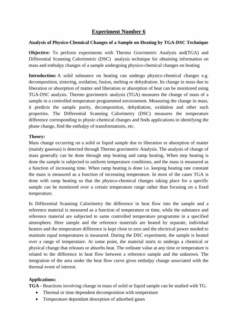
Experiment Number 6
Analysis of Physico-Chemical Changes of a Sample on Heating by TGA-DSC Technique
Objective: To perform experiments with Thermo Gravimetric Analysis and(TGA) and Differential Scanning Calorimetric (DSC) analysis technique for obtaining information on mass and enthalpy changes of a sample undergoing physico-chemical changes on heating
Introduction: A solid substance on heating can undergo physico-chemical changes e.g. decomposition, sintering, oxidation, fusion, melting or dehydration. Its change in mass due to liberation or absorption of matter and liberation or absorption of heat can be monitored using TGA-DSC analysis. Thermo gravimetric analysis (TGA) measures the change of mass of a sample in a controlled temperature programmed environment. Measuring the change in mass, it predicts the sample purity, decomposition, dehydration, oxidation and other such properties. The Differential Scanning Calorimetry (DSC) measures the temperature difference corresponding to physic-chemical changes and finds applications in identifying the phase change, find the enthalpy of transformations, etc.
Theory: Mass change occurring on a solid or liquid sample due to liberation or absorption of matter (mainly gaseous) is detected through Thermo gravimetric Analysis. The analysis of change of mass generally can be done through step heating and ramp heating. When step heating is done the sample is subjected to uniform temperature conditions, and the mass is measured as a function of increasing time. When ramp heating is done i.e. keeping heating rate constant the mass is measured as a function of increasing temperature. In most of the cases TGA is done with ramp heating so that the physico-chemical changes taking place for a specific sample can be monitored over a certain temperature range rather than focusing on a fixed temperature.
In Differential Scanning Calorimetry the difference in heat flow into the sample and a reference material is measured as a function of temperature or time, while the substance and reference material are subjected to same controlled temperature programme in a specified atmosphere. Here sample and the reference materials are heated by separate, individual heaters and the temperature difference is kept close to zero and the electrical power needed to maintain equal temperatures is measured. During the DSC experiment, the sample is heated over a range of temperature. At some point, the material starts to undergo a chemical or physical change that releases or absorbs heat. The ordinate value at any time or temperature is related to the difference in heat flow between a reference sample and the unknown. The integration of the area under the heat flow curve gives enthalpy change associated with the thermal event of interest. Applications: TGA - Reactions involving change in mass of solid or liquid sample can be studied with TG.
Thermal or time dependent decomposition with temperature
Temperature dependant desorption of adsorbed gases
Fusion and evaporation of water associated with the sample
Combustion reactions
DSC- It is the most widely used thermal analysis technique since it gives the measure of heat flow associated with endothermic or exothermic transitions. Thus it is useful to study reaction thermodynamics as well as kinetics. The transitions usually traced by the technique are as follows:
Glass transition temperature, crystallization temperature, melting temperature and associated enthalpy changes for a polymer
Phase change
Product stability
Frequently used in industry to measure glass transition temperature and %crystallization of polymer.
Apparatus:TGA The TGA part of the TGA-DSC apparatus and has following four major components;
The electro-balance and its controller: e.g. Null point weighing mechanism.
The furnace and temperature sensors: e.g. MoSi2 based furnace with alumina refractories and a thermocouple Pt-30%Rh (+) Vs Pt-6%Rh (-) for operation to 1500 to 1700 0C.
Purge gas flow controller
The programmer or computer
The data acquisition device
Apparatus: DSC The major parts of the DSC part of the system are;
The DSC sensor plus amplifier
The furnace and its temperature sensor
The programmer or computer
The data acquisition device
Instrument Detail
Company: M/s. NETZSCH Gerabau GmbH
Model: Simultaneous TGS-DSC Apparatus STA 409/PC/4/H/LUXX
Temperature range: 25o – 16500C
Heating and cooling rate: 0.01 K/min to 50 K/min (dependent on furnace) generally operated at 10K/min.
The balance: can weigh maximum of 50 mg.
Resolution: The resolution of TG instrument is 2 μg.
Operating Atmosphere: inert, oxidizing, reducing, static, dynamic.
Simultaneous TG-DSC apparatus
Experimental Procedure:
Power unit, Furnace unit, Gas control unit, Water circulation unit were switched on in the respective order.
Pressure from the connected gas line N2/O2/air should be maintained around 1kgf/cm2 and gas lines should be turned on. Baseline correction
Reference and analysis pan was cleaned manually and the weight was taken.
Furnace unit was opened using PUSH UP+ SAFETY buttons. Pan was placed over the sensors using forks and their weights were noted down.
Baseline correction was performed in the same program which is used to generate results.
The software STA409PC was opened.
Under Measurements CORRECTION was marked.
Entered Sample ID and name.
Tare sample crucible and reference crucible mass by clicking “weigh” button.
Kept the reference mass blank.
Under PURGE GAS Gas1 (N2) flow: 40ml/min and Gas2 (N2) flow: 60ml/min were set.
After pressing continue, calibration file were selected from source NEW-DTA-CAL-N2 and sensitivity file from source SENSCAL-AL2O3-N2.ESV.
Multiple tabs got opened.
Under step conditions: The check box for STC, GAS 1 and GAS 2 were selected.
Under Category Initial Temperature Conditions were set to 260C.
ADD to END was pressed to close the TAB.
In side bar DYNAMIC was selected and Under Category End Temperature and the Heating Rate (Acquisition rate in points/K and in points/min will be taken automatically) were entered.
ADD to END was repressed to end the tab.
In the graph generated in the screen all of these got added.
In side bar FINAL was selected and the final temperature is automatically taken 100C more than the end temperature by the instrument. This is the emergency reset temperature.
In the specified path the file was saved and named. All the above settings were saved there as baseline correction.
COM1 WINDOW appeared soon after a minute.
Pressed initial condition on.
Gas flow in the rotameter was checked.
TARE tab was pressed.
Then START tab was pressed. Program got started and data acquisition started to take place.
Precautions:
1. Total mass of the sample taken should be in the range of 10-20 mg. Within this range temperature distribution remains uniform.
2. As hands contain moisture no hand contact should be made with the crucible. It might change the reading. Some moisture will add up the mass.
3. To get a stable weight in the electrobalance the instrument should be turned on an hour before the experiment.
4. Once the desired temperature rate is achieved the instrument is allowed to cool down to room temperature. Else when the heated instrument remains exposed to the open atmosphere due to the large temperature difference sensitivity of the thermocouple might be damaged.
5. After the completion of the experiment the pans should be washed properly to get rid of minute traces of residues.
References
1. Brown, M. E. (Ed.), 2007, “Introduction to Thermal Analysis: techniques and Applications”, 2nd Edition, Springer, New Delhi, 1-90. 2. Price, D. M., Hourston, D. J. and Dumont, F. 2000, “Thermogravimetry of Polymers” in “Encyclopaedia of Analytical Chemistry” edited by Meyers R.A., John Wiley &
Sons Ltd, Chichester, 8094–8105.