experimental characterization of baffle plate influence on
TRANSCRIPT

Brigham Young University Brigham Young University
BYU ScholarsArchive BYU ScholarsArchive
Theses and Dissertations
2011-06-14
Experimental Characterization of Baffle Plate Influence on Experimental Characterization of Baffle Plate Influence on
Turbulent and Cavitation Induced Vibrations in Pipe Flow Turbulent and Cavitation Induced Vibrations in Pipe Flow
Gavin J. Holt Brigham Young University - Provo
Follow this and additional works at: https://scholarsarchive.byu.edu/etd
Part of the Mechanical Engineering Commons
BYU ScholarsArchive Citation BYU ScholarsArchive Citation Holt, Gavin J., "Experimental Characterization of Baffle Plate Influence on Turbulent and Cavitation Induced Vibrations in Pipe Flow" (2011). Theses and Dissertations. 2765. https://scholarsarchive.byu.edu/etd/2765
This Thesis is brought to you for free and open access by BYU ScholarsArchive. It has been accepted for inclusion in Theses and Dissertations by an authorized administrator of BYU ScholarsArchive. For more information, please contact [email protected], [email protected].
Experimental Characterization of Baffle Plate Influence
on Turbulent and Cavitation Induced
Vibrations in Pipe Flow
Gavin J. Holt
A thesis submitted to the faculty of Brigham Young University
in partial fulfillment of the requirements for the degree of
Master of Science
R. Daniel Maynes, Chair Jonathan D. Blotter Steven L. Gorrell
Department of Mechanical Engineering
Brigham Young University
June 2011
Copyright © 2011 Gavin J. Holt
All Rights Reserved


ABSTRACT
Experimental Characterization of Baffle Plate Influence on Turbulent and Cavitation Induced
Vibrations in Pipe Flow
Gavin J. Holt Department of Mechanical Engineering
Master of Science
Turbulent and cavitation induced pipe vibration is a large problem in industry often resulting in pipe failures. This thesis provides an experimental investigation on turbulent flow and cavitation induced pipe vibration caused by sharp edged baffle plates. Due to large pressure losses across a baffle plate, cavitation can result. Cavitation can be destructive to pipe flow in the form of induced pipe wall vibration and cavitation inception. Incipient and critical cavitation numbers are design points that are often used in designing baffle plate type geometries. This investigation presents how these design limits vary with the influencing parameters by exploring a range of different baffle plate geometries. The baffle plates explored contained varying hole sizes that ranged from 0.159 cm to 2.54 cm, with the total through area, or openness, of each baffle plate ranging between 11% and 60%. Plate thickness varied from 0.32-0.635 cm. Reynolds numbers ranged from 5 x 10⁴-85 x 104
Keywords: Gavin Holt, flow, fluids, vibration, vibrations, cavitation, flow, induced, pipes, pipe,fluid structure, inception, attenuation, loss coefficient, baffle plate, multi-hole orifice, flow rate, pipe flow, turbulence, turbulent, discharge coefficient, size scaling
. The results show that the cavitation design limits are function of size scale effects and the
loss coefficient only. The results also show that the loss coefficient for a baffle plate varies not only with total through area ratio, but also due with the plate thickness to baffle hole diameter ratio. Pipe wall vibrations were shown to decrease with increased through area ratio and increased thickness to diameter ratios.
An investigation was also performed to characterize the attenuation of vibration in the
streamwise direction of a baffle plate. It was show that the attenuation was largely effected by the presence of cavitation. Attenuation was shown to be a function of the geometry of the baffle plate.
This work resulted in empirical models that can be used for predicting pipe vibration
levels, the point of cavitation inception, and the streamwise distance where the attenuation of vibration levels caused by a baffle plate occurs.


ACKNOWLEDGMENTS
I would first like to thank Dr. Daniel Maynes for his time, insight, and guidance. The
time that he sacrificed and provided has not only given me increased confidence and knowledge
but gave the needed guidance to produce the results of this thesis. The knowledge I gained
working alongside this man was priceless.
I would also like to thank Dr. Jonathan Blotter for his time and guidance given. Without
his interest in the project and his insight, this work would not have been able to move forward.
This work was funded by Control Components Inc. Their interest in this work has
provided the funding for my education and means for this work to go forth.
Finally I would like to thank my family for the time they sacrificed and their patience
with me. I would especially like to thank my wife Shauna for enduring with me and her
motivational love and support.


v
TABLE OF CONTENTS
LIST OF TABLES ....................................................................................................................... ix
LIST OF FIGURES ..................................................................................................................... xi
1 Introduction ........................................................................................................................... 1
1.1 Research Objectives ........................................................................................................ 5
1.2 Project Scope .................................................................................................................. 5
1.3 Overview ......................................................................................................................... 6
2 Background ........................................................................................................................... 7
2.1 Turbulence Induced Vibrations ...................................................................................... 7
2.2 Baffle Plate Loss Coefficient .......................................................................................... 8
2.2.1 Detached Model (Thin Baffle Plate) ......................................................................... 10
2.2.2 Attached Model (Thick Plate) ................................................................................... 13
2.3 Cavitation and Cavitation Induced Vibrations .............................................................. 15
2.4 Literature Review ......................................................................................................... 22
2.4.1 Turbulent Induced Pipe Vibrations ........................................................................... 22
2.4.2 Cavitation Induced Pipe Vibrations .......................................................................... 24
2.5 Current State of the Art ................................................................................................. 27
2.6 Research Contributions ................................................................................................. 28
3 Experiment Setup ................................................................................................................ 31
3.1 Flow Loop ..................................................................................................................... 31
3.2 Baffle Plates .................................................................................................................. 35
3.3 Instrumentation ............................................................................................................. 36
4 Experimental Procedures ................................................................................................... 39
4.1 Measurements of Cavitation Inception and Pipe Vibrations ........................................ 39

vi
4.2 Data Analysis of Cavitation and Pipe Vibrations ......................................................... 40
4.3 Measurements of Attenuation of Pipe Vibrations ......................................................... 45
4.4 Data Analysis of Attenuation of Pipe Vibrations ......................................................... 46
4.5 Uncertainty Analysis ..................................................................................................... 46
4.5.1 Regression Analysis Uncertainty .............................................................................. 47
4.5.2 Measurement Uncertainty ......................................................................................... 48
4.5.3 Calculated Variables Uncertainty ............................................................................. 49
5 Characterized Results ......................................................................................................... 53
5.1 Baffle Loss Coefficient ................................................................................................. 53
5.2 Characterization of Vibrations and Incipient Cavitation .............................................. 56
5.3 Characterized Attenuated Vibrations ............................................................................ 64
5.4 Summary of Observations from the Results ................................................................. 68
6 Developed Models ............................................................................................................... 69
6.1 Loss Coefficient ............................................................................................................ 70
6.2 Incipient and Critical Cavitation Numbers ................................................................... 73
6.3 A′ at Critical and Incipient Cavitation ........................................................................... 79
6.4 The Incipient and Critical Velocities ............................................................................ 83
6.5 Slope for Non-Cavitating Regime ................................................................................ 86
6.6 Attenuation of Vibration ............................................................................................... 89
7 Conclusions .......................................................................................................................... 91
7.1 Summary of Results ...................................................................................................... 91
7.2 Recommendations ......................................................................................................... 92
REFERENCES ............................................................................................................................ 93
Appendix A. Instructions on Use of Models .......................................................................... 95
Appendix B. Key Parameters for all Baffle Plates Considered ......................................... 101

vii
Appendix C. MATLAB Code for Post Processing .............................................................. 103
Appendix D. MATLAB Code for Attinuation Data ........................................................... 105


ix
LIST OF TABLES
Table 1: Baffle plates used in the study with baffle hole diameter, number of baffle holes,
and baffle plate thickness shown. ....................................................................................35
Table 2: The maximum variation in the two different independent tests that were conducted for every scenario for the variables that was determined at both incipient and critical cavitation as seen below. ......................................................................................40
Table 3: Uncertainty in determining design limits ......................................................................48
Table 4: Key parameters for all baffle plates considered ............................................................101

xi
LIST OF FIGURES
Figure 1: Typical baffle plate used ..............................................................................................1
Figure 2: Illustration of Turbulent and cavitatating flow through a baffle plate. An illustration of the vena-contracta through one hole in a baffle plate is also depicted. .....3
Figure 3: Rupture due to vibration induced fatigue caused an oil spill in Cohasset, Minnesota. The top image shows an image of the area of the oil spill and the bottom image shows the one mile smoke plume. [3] ...................................................................4
Figure 4: Turbulent jets interacting ..............................................................................................8
Figure 5: Illustration of a single baffle hole showing the vena-contracta region within the baffle hole. .......................................................................................................................10
Figure 6: Illustration of a flow through a thin baffle hole when flow does not reattach after the vena-contracta (detached flow). .................................................................................11
Figure 7: Control volume for sudden contraction for a detached jet ...........................................12
Figure 8: Control volume within baffle hole with attached jet. ...................................................14
Figure 9: Control volume for a sudden contraction area when the flow reattaches within the baffle plate .......................................................................................................................15
Figure 10: Example of cavitation bubble formation within the shear layer from a baffle plate within a pipe section from [16]. ..............................................................................17
Figure 11: (Top) Illustration of the pressure variation across a sudden contraction and then sudden expansion. (Bottom) A schematic illustration of the vena-contracta section of a sudden contraction/sudden expansion (baffle plate) with reattachment of the flow occuring after the vena-contracta. ...........................................................................18
Figure 12: A representative plot of A′ vs. the cavitation number, σ, showing four different cavitation regimes. The black line is the non-cavitating regime, the red line is the incipient cavitation regime, the blue line is the fully cavitating regime, and the green line is the choked cavitating regime. The intersection of the red and black lines is the incipient cavitation design limit, σi, the intersection of the blue and red lines is the critical cavitation design limit, σc. and the intersection of the green and blue lines is the chocked cavitation design limit, σch .......................................................20
Figure 13: Pipe wall acceleration vs. downstream distance normalized by the pipe diameter, x/D, for 5 baffle plates with varying hole diameters and a no baffle plate case as measured by Thompson as shown in the legend [7]. .......................................................23

xii
Figure 14: A plot of the pipe wall acceleration, A′, vs. the average pipe fluid velocity, vp, for 5 baffle plates with varying baffle hole diameters that were used by Thompson as shown in the legend [7]. .............................................................................................25
Figure 15: Power spectral density, �̂�𝐴U, vs. frequency, f, for five baffle plates with varying baffle hole diameters studied by Thompson [7], as shown in the legend, at a flow speed of 5.63 m/s measured at 0.305 m downstream from the baffle plate. ....................26
Figure 16: A plot of inception cavitation number vs. discharge coefficient for 4 multi-hole orifice plates used by Tullis et. al. [9] ..............................................................................27
Figure 17: Schematic drawing of the flowloop facility used for all experiments. .......................32
Figure 18: Photograph of the centrifugal pump and flow conditioner used in flow loop facility. Downstream of the flow conditioner the rubber coupler and developing region can be seen. ...........................................................................................................32
Figure 19: Photograph of the pipe test section showing the location of the thermocouple and flow meter relative to the test section. ......................................................................34
Figure 20: Photograph of a baffle plate mounted between the developing region and test section. The locations of the upstream and downstream pressure transducers along with microphone and accelerometer are also shown. ......................................................34
Figure 21: Photographs of the sixteen baffle plates used in the study, showing arranged in the same order as Table 1 from left to right and top to bottom. ......................................36
Figure 22: Ln(A′) vs. Ln(vH) used to obtain inception and critical cavitation values. Values of the coefficients m and b for the linear form y=mx+b are shown for each of the three linear regimes. .........................................................................................................42
Figure 23: Ln(A′) vs. Ln(σ) used to obtain inception and critical cavitation values. Values of the coefficients m and b for the linear form y=mx+b are shown for each of the three linear regimes. .........................................................................................................43
Figure 24: Ln(A′) vs. Ln(σv) used to obtain inception and critical cavitation values. Values of the coefficients m and b for the linear form y=mx+b are shown for each of the three linear regimes. .........................................................................................................43
Figure 25: A representative plot of 𝐴𝐴2′∗ vs. x/D for four different baffle hole velocities for
one baffle plate. The x markings indicate 1.5 time the no baffle plate vibrations. .........47
Figure 26: Loss coefficient, KLH, vs. the total through area ratio, AH/Ap, for 16 baffle plates. Included is a theoretical attached model, KLA, and a theoretical detached model, KLD. Data from Testud et. al. is also included for comparison. ..........................55
Figure 27: Loss coefficient, KLH, vs. the thickness ratio, t/d, for 16 baffle plates and four area ratios as shown in the legend. ...................................................................................56

xiii
Figure 28: A′ vs. average baffle hole velocity, vH, for five baffle plates of constant through area (AH/Ap=0.438) and five different t/d ratios as shown in the legend. ........................58
Figure 29: A′ vs. average baffle hole velocity, vH, for five baffle plates of nominally constant through area (AH/Ap=0.219) and five different t/d ratios as shown in the legend. ..............................................................................................................................58
Figure 30: A′ vs. average baffle hole velocity, vH, for four baffle plates of constant thickness ratio (t/d=1.7) and four different through areas (AH/Ap) as shown in the legend. ..............................................................................................................................59
Figure 31: A′ vs. average baffle hole velocity, vH, for four baffle plates of constant thickness ratio (t/d=1) and four different through areas (AH/Ap) as shown in the legend. ..............................................................................................................................60
Figure 32: A′ vs. the cavitation number, σ, for five baffle plates of constant through area (AH/Ap=0.219) and five different thickness ratios as shown in the legend. .....................61
Figure 33: Incipient cavitation number vs. t/d for 14 baffle plates and three different through area ratios. ...........................................................................................................62
Figure 34: Incipient cavitation number vs. AH/Ap for 14 baffle plates and five different t/d ratios. ................................................................................................................................63
Figure 35: 𝐴𝐴2′∗
U vs. x/D for the baffle plate with a hole diameter of 0.634 cm and 28 holes and at four different average baffle hole velocities as shown in the legend. Open markers indicate that cavitation is occurring, and closed markers correspond to the non-cavitating regime. .....................................................................................................65
Figure 36: 𝐴𝐴2′∗
U vs. x/D for the baffle plate with a hole diameter of 0.634 cm and 112 holes and at four different average baffle hole velocities as shown in the legend. Open markers indicate that cavitation is occurring, and closed markers correspond to the non-cavitating regime. .....................................................................................................66
Figure 37: 𝐴𝐴2′∗
U vs. x/D for five baffle plates with varying baffle hole diameter, d, with constant through area ratio (AH/Ap=0.438) and constant baffle hole velocity (vH = 10.7 m/s). Open markers indicate that cavitation is occurring, and closed markers correspond to the non-cavitating regime. .........................................................................67
Figure 38: A representative plot of A′ vs. the cavitation number, σ. The intersection of the red and black lines is the incipient cavitation design limit, σi, and the intersection of the blue and red lines is the critical cavitation design limit, σc . ......................................70
Figure 39: The ratio of the actual loss coefficient over the theoretical loss coefficient, KLH/KLA, vs. 𝜙𝜙U for 14 baffle plates along with data taken by Testud et. al. (2007) as shown in the figure legend. ..............................................................................................72
xiv
Figure 40: The actual loss coefficient, KLH, vs. the modeled KLH of Eq. (5.5). The goodness of fit is shown with an R2 value of 0.967. ........................................................73
Figure 41: The incipient cavitation number with size scale effects, σi, vs. the discharge coefficient, cd for 13 baffle plates. Data taken by Testud et. al. (2007) [13] is also shown. The open data point is a baffle plate that had slight chamfers for each of the baffle holes. ......................................................................................................................76
Figure 42: A plot of the actual incipient cavitation number with size scale effects, 𝜎𝜎𝑖𝑖∗, vs. the developed model of Eq. (5.13) with an R2 value equal to 0.997 as shown in figure. ...............................................................................................................................76
Figure 43: The critical cavitation number with size scale effects, 𝜎𝜎𝑐𝑐∗, vs. the discharge coefficient, cd for 13 baffle plates. The open data point is a baffle plate that had slight chamfers for each of the baffle holes. ....................................................................77
Figure 44: A plot of the actual critical cavitation number with size scale effects, 𝜎𝜎𝑐𝑐∗, vs. the developed model of Eq. (5.14) with an R2 value equal to 0.978 as shown in figure. ......77
Figure 45: The incipient cavitation number with size scale effects, 𝜎𝜎𝑖𝑖∗, vs. the discharge coefficient, cd for 13 baffle plates. Data taken by Testud et. al. (2007) [13], data from Tullis et. al. (1980) [9] for multi-hole orifice plates with rounding of 0.9525 cm for the inlet of each hole, and data from Tullis (1989) [15] for a single hole orifice is also shown. The open circle data point is an outlier caused by a baffle plate that had slight chamfers for each of the baffle holes. ............................................78
Figure 47: A plot of the actual 𝐴𝐴𝑖𝑖′∗ vs. the model developed in Eq. (5.17) with an R2 value equal to 0.964 as shown in figure. ...................................................................................81
Figure 48: ln(𝐴𝐴𝑐𝑐′∗) as a function of βc for 12 baffle plate. ............................................................82
Figure 49: A plot of the actual 𝐴𝐴𝑐𝑐′∗vs. the model developed in Eq. (5.18) with an R2 value equal to 0.984 as shown in figure. ...................................................................................82
Figure 50: The pipe velocity at critical cavitation, vpi, vs. ψ for 13 baffle plates. .....................84
Figure 51: The pipe velocity at critical cavitation, vpc, vs. ψ for 13 baffle plates. ....................85
Figure 52: A plot of the actual vpi vs. the model developed in Eq. (5.26) showing an R2 value equal to 0.981 as shown in figure. ..........................................................................85
Figure 53: A plot of the actual vpc vs. the model developed in Eq. (5.27) showing an R2 value equal to 0.985 as shown in figure. ..........................................................................86
Figure 54: A plot of the m* as a function of ε for 14 baffle plates ............................................88
Figure 55: A plot of the actual m* value vs. the model developed in Eq. (5.23) showing an R2 value equal to 0.976 as shown in figure. .....................................................................88

xv
Figure 56: The attenuation of vibration levels downstream of the baffle plate, x/D, vs. Re/Rei . ..............................................................................................................................90
Figure 57: Plot of sigma vs. 𝐴𝐴′ showing the two design limits that have been solved from the example problem in section 4.7 .................................................................................99
Figure 58: Plot of A′ vs. σ comparing experimental results to a model that was developed in equation (A.31) for a baffle plate with d=0.634 t=0.67 and n=112. ...............................100


xvii
NOMENCLATURE
A′ RMS of pipe wall acceleration (m/s2
𝐴𝐴𝑐𝑐′
)
RMS of pipe wall acceleration at critical cavitation (m/s2
𝐴𝐴𝑖𝑖′
)
RMS of pipe wall acceleration at inception (m/s2
𝐴𝐴′∗
)
Non-dimensionalized A′, 𝐴𝐴′𝑑𝑑vH
2 (-)
𝐴𝐴2′∗ Non-dimensionalized A′, 𝐴𝐴
′ 𝐷𝐷𝑣𝑣𝑝𝑝2
(-)
𝐴𝐴𝑐𝑐′∗ Non-dimensionalized A′ at critical cavitation, 𝐴𝐴𝑐𝑐′ 𝑑𝑑
𝑣𝑣𝐻𝐻𝑐𝑐 2 (-)
𝐴𝐴𝑖𝑖′∗ Non-dimensionalized A′ at inception, 𝐴𝐴𝑖𝑖
′ 𝑑𝑑𝑣𝑣𝐻𝐻𝑖𝑖
2 (-)
A Total baffle hole area, 𝜋𝜋𝑛𝑛𝑑𝑑2
4 (mH
2
A
)
Total area made from the jets of the vena-contracta (mj 2
A
)
Pipe area (mp 2
c
)
Discharge coefficient (-) d
D Pipe diameter (m)
d Baffle hole diameter (m)
𝐾𝐾𝐿𝐿𝐻𝐻 Loss coefficient based on baffle hole velocity, 𝑃𝑃1−𝑃𝑃21/2𝜌𝜌𝑣𝑣𝐻𝐻
2 (-)
𝐾𝐾𝐿𝐿𝑝𝑝 Loss coefficient based on the pipe velocity, 𝑃𝑃1−𝑃𝑃21/2𝜌𝜌𝑣𝑣𝑝𝑝2
(-)
𝐾𝐾𝐿𝐿𝐴𝐴 Theoretical loss coefficient for a thick plate (-)
𝐾𝐾𝐿𝐿𝐷𝐷 Theoretical loss coefficient for a thin (-)
m Slope of the non-cavitating regime for 𝐴𝐴′ vs. cavitation number with log-log scale (-)
l length of the developing section (m) e
m Slope of the incipient regime for 𝐴𝐴′ vs. cavitation number with log-log scale (-) 2
m* A normalized slope value, 𝑚𝑚
2 𝑙𝑙𝑛𝑛�𝐴𝐴𝐻𝐻𝐴𝐴𝑝𝑝�−0.4
(-)
n Number of baffle holes (-)

xviii
P Upstream pressure (Pa) 1
P Downstream pressure (Pa) 2
P Jet pressure (Pa) j
P Vapor pressure (Pa) v
Re Reynolds number, 𝜌𝜌𝑣𝑣𝑝𝑝𝐷𝐷𝜇𝜇
(-) D
SSE Size scale effects for the cavitation number, �𝐷𝐷𝑑𝑑�𝑌𝑌 (-)
t Baffle plate thickness (m)
v Average baffle hole fluid velocity (m/s) H
v Average baffle hole fluid velocity at critical cavitation (m/s) Hc
v Average baffle hole fluid velocity at cavitation inception (m/s) Hi
v Average jet velocity (m/s) j
v Average pipe fluid velocity (m/s) p
v Average pipe fluid velocity at critical cavitation (m/s) pc
v Average pipe fluid velocity at cavitation inception (m/s) pi
x Streamwise distanced from baffle plate (m)
Y A scaling factor used for, 0.3𝐾𝐾𝐿𝐿𝑝𝑝−0.25 (-)
𝛼𝛼 Vena-contracta contraction ratio, 𝐴𝐴𝑗𝑗𝐴𝐴𝐻𝐻
(-)
𝛽𝛽𝑖𝑖 A non-dimensional number, 𝜎𝜎𝑖𝑖 �𝑡𝑡𝑑𝑑�
1.8�𝐴𝐴𝐻𝐻𝐴𝐴𝑝𝑝�−0.6
(-)
𝛽𝛽𝑐𝑐 A non-dimensional number, 𝜎𝜎𝑐𝑐 �𝑡𝑡𝑑𝑑�
1.8�𝐴𝐴𝐻𝐻𝐴𝐴𝑝𝑝�−0.6
(-)
𝜖𝜖 A non-dimensional number, �𝑑𝑑𝐷𝐷� �𝑡𝑡
𝑑𝑑�
0.4�𝐴𝐴𝐻𝐻𝐴𝐴𝑝𝑝�
2.5 (-)
𝜇𝜇 Fluid dynamic viscosity (N s/m2)

xix
𝜙𝜙 �𝑡𝑡𝑑𝑑� �𝐴𝐴𝐻𝐻
𝐴𝐴𝑝𝑝�
1/5 (-)
𝜓𝜓 𝑐𝑐𝑑𝑑 �𝑡𝑡𝑑𝑑�
0.15 (-)
𝜌𝜌 Fluid density (kg/m3
σ
)
Cavitation number, 𝑃𝑃2−𝑃𝑃𝑣𝑣𝑃𝑃1−𝑃𝑃2
(-)
σ Critical cavitation number (-) c
σ Choked cavitation number (-) ch
σ Incipient cavitation number (-) i
𝜎𝜎𝑐𝑐∗ σc
𝜎𝜎𝑖𝑖∗
SSE (-)
σi
SSE (-)


1
1 INTRODUCTION
Many industries rely heavily upon pipe systems. These systems may result in vibration
induced fatigue failure if prolonged vibration loading prevails. Vibration fatigue of a pipe can
be a result of fluid induced vibrations or mechanical induced vibrations. Fluid induced vibrations
are the result of large pressure surges (such as water hammer), cavitation, and turbulent flows.
The focus of this work is turbulence and cavitation induced vibrations that result from multi-
holed baffle plates in a pipe system. A baffle plate is a thin metal plate with multiple holes, with
the number of holes varying depending on the desired flow rates through the system. Figure 1 is
an image of a baffle plate that was used in this study. Baffle plates can be used to model high
pressure drop valve systems that often have similar geometries and are used to control pressure
drop in the system. Due to the intrusive nature of the baffle plates, high levels of turbulence and,
when high flow rates are achieved, cavitation can occur.
Figure 1: Typical baffle plate used

2
Cavitation is the generation of small vapor bubbles within a liquid system, similar to
boiling. It results due to the local static pressure dropping below the vapor pressure. In the case
of a baffle plate, as the fluid approaches the baffle hole it accelerates causing the pressure to
drop. If the pressure drops below the vapor pressure, vapor bubbles then form and convect
downstream where the pressure then increases. With this increase in pressure the vapor bubbles
are forced to collapse upon themselves releasing high amounts of acoustical energy that cause
pipe vibrations. The vibrations caused by cavitation can be orders of magnitudes greater than the
vibration level that exists when cavitation is not present.
In Figure 2 an illustration of the physical occurrence through a baffle plate is shown. As
the flow passes through the baffle plate it forms what is referred to as a vena-contracta. As the
fluid exits the baffle plate it forms multiple turbulent liquid jets and shear layers where high
levels of turbulence production is occurring. When cavitation is present vapor regions occur
within the liquid jets. As is depicted in the illustration, the jets interact with each other whether
or not cavitation is present. For this reason the geometric dimensions of the baffle plate have a
large effect on the level of turbulence and cavitation that is produced.
As was mentioned above, industrial systems may fail due to the turbulent and cavitation
induced vibrations. The result of such failures may result in tremendous cost in both time and
money. At present, the needed information and tools necessary for a designer to take in account
the loading caused by cavitation and turbulence induced vibrations for flow through multi-holed
baffle plates are not available.

3
Figure 2: Illustration of Turbulent and cavitatating flow through a baffle plate. An illustration of the vena-contracta through one hole in a baffle plate is also depicted.
Within the nuclear industry vibration induced fatigue is one of the predominate failures
of pipe systems [1]. In a nuclear power plant in Daya Bay China, within only eight years of
operations, the plant launched a research project because vibration induced fatigue was
occurring. The outcome of the research showed that cavitation, which occurred from the
pressure drop over an orifice plate, was the source to the vibration induced fatigue failures [2].
In Cohasset Minnesota on July 4, 2002 a pipe ruptured due to vibration induced fatigue,
releasing three thousand barrels of crude oil. The repair and cleanup costs were about $5.6
million [3]. Figure 3 shows the oil spilled from the failed pipe system illustrating the impact of
this event.

4
Figure 3: Rupture due to vibration induced fatigue caused an oil spill in Cohasset, Minnesota. The top image shows an image of the area of the oil spill and the bottom image shows the one mile smoke plume. [3]
The focus of this work is to produce the needed information and predictive tools
necessary for the design and maintenance of valve and pipe systems where baffle plate type
geometries are encountered. Such tools will lead to improved future designs of industrial pipe
systems, leading to reduced failures and saving millions of dollars.

5
1.1 Research Objectives
Four main objectives of this research are outlined below:
1. Perform experiments that characterize the inception of cavitation in terms of baffle plate
variables, such as baffle hole diameter, baffle plate thickness, through area ratio, baffle
hole spacing, fluid velocity, etc.
2. Conduct experiments that characterize the concomitant pipe acceleration as a function of
the influencing parameters.
3. Conduct experiments that characterize the streamwise distance downstream where the
attenuation of pipe wall vibrations caused by a baffle plate occurs, as a function of baffle
hole diameter, through area ratio, hole spacing, plate thickness, fluid velocity, etc.
4. Produce predicted models that can be used in design and modification of industrial
systems.
1.2 Project Scope
The scope of this research was to investigate experimentally the influence of sharp-edged
baffle plates on pipe vibration and to produce predictive models that characterize the
experimental results. The primary parameters of significance that were studied were: baffle hole
diameter, number of baffle holes, fluid kinetic energy in the baffle holes, bulk fluid flow rate,
baffle plate thickness, and baffle plate pressure loss coefficient.
This work was limited to flow through a pipe diameter of 10.16 cm. The range of baffle
plate geometries was limed to baffle hole diameters ranging from 0.16-2.54 cm and through area
ratios ranging from 10.9%-60.9%. The range of baffle fluid velocities was limited to flow
speeds below 20.2 m/s.
6
1.3 Overview
Chapter 2 provides a detailed background into turbulent and cavitation induced pipe
vibrations including a section on a review of the relevant literature and the current state of the
art. Concluding Chapter 2 is a discussion of the contributions this work provides relative to the
current state of the art. Chapter 3 gives a detailed description of the flow facilities used to
perform experimentation. This chapter will also discuss the specific geometries of the baffle
plates used for this work. Chapter 3 will concluded with a discussion of the instrumentation that
was used. Chapter 4 describes the experimental procedures carried out. It also discusses the
methods used for data analysis and provides uncertainty analysis of all measured parameters.
Chapter 5 presents the results from the experimental investigation. Discussing the general
turbulent and cavitation induced pipe vibration behavior, and the attenuation of the pipe
vibrations with downstream distance will be discussed. Chapter 6 will present and discuss the
predictive models that were developed. Chapter 7 provides a summary of the work performed
and summarizes the conclusions of the research. Chapter 7 concludes with a section on
recommendations for future work in this area.

7
2 BACKGROUND
This section provides background and a literature review of previous work on flow
induced vibrations and cavitating flow in multi-holed baffle plates. First, characterization of
turbulent induced vibrations will be discussed. Second, a discussion on the influences of the loss
coefficient will be provided. This is important because the loss coefficient strongly relates to
cavitation inception and pipe vibrations. Lastly, a discussion of cavitation and its effects on pipe
vibrations will be given.
2.1 Turbulence Induced Vibrations
Turbulence is defined by Von Karman as “…an irregular motion [4].” Turbulence is
caused by a fluid reaching high enough Reynolds numbers that the viscous stresses are overcome
by the fluid inertia. Fluctuating pressure and velocities then prevail and the motion becomes
inherently three dimensional and unsteady [4].
Within the boundary layer fluid structures called eddies, or vortices, are generated.
Eddies are defined as local swirling motion [4]. These structures have a large range of sizes and
carry large amounts of energy [4]. As the flow rate increases so does the turbulence or
generation of these vortices. Due to the no-slip condition, as the vortices approach the wall of
the pipe, the kinetic energy that they are carrying must be converted to some other energy source
according to the first law of thermodynamics. This energy is converted to heat and pressure
fluctuations [5].

8
For turbulent induced pipe vibrations that occur under fully-developed turbulent flow
conditions without a baffle plate, it has been shown experimentally and analytically that both the
pressure fluctuations and the pipe wall acceleration scale with the square of the average pipe
fluid velocity [6,7,8,5].
Figure 4 is an illustration of two turbulent jets interacting. Where the shear layers of the
two jets interact the velocity of the rotational flow in the dominant turbulent eddies of the two
jets are opposite. This can cause suppression to the levels of turbulence [9]. Because of this it is
believed that with increased amounts of interacting jets the pipe wall vibrations will decrease.
Figure 4: Turbulent jets interacting
2.2 Baffle Plate Loss Coefficient
Ball stated that the pressure drop across an orifice plate is caused by the pressure head on
the plate, the losses due to friction, and the losses due to turbulence disturbances [10]. It was
shown in a study performed by Kolodzie et. al. that loss, when considering multi-hole orifice

9
plates, was influenced by the hole diameter, through area ratio, and the pitch to diameter ratio
[11].
The loss coefficient for baffle plate can be defined as the ratio of the upstream pressure
minus the downstream pressure all divided by the dynamic pressure as shown in equation (2.1)-
(2.2) [12]. Equation (2.2) is defined with the average fluid pipe velocity, vp (2.2), and equation
is defined with the average fluid baffle hole velocity, vH. By using conservation of mass these
two equations can be related by the through area ratio, AH/Ap, (2.3)as shown in equation . AH is
the total area of all the baffle holes and Ap
𝐾𝐾𝐿𝐿𝑝𝑝 =𝑃𝑃1 − 𝑃𝑃2
1/2𝜌𝜌𝑣𝑣𝑝𝑝2
is the pipe cross-sectional area.
(2.1)
𝐾𝐾𝐿𝐿𝐻𝐻 =𝑃𝑃1 − 𝑃𝑃2
1/2𝜌𝜌𝑣𝑣𝐻𝐻2 (2.2)
𝐾𝐾𝐿𝐿𝐻𝐻 = 𝐾𝐾𝐿𝐿𝑝𝑝 �𝐴𝐴𝐻𝐻𝐴𝐴𝑝𝑝�
2
(2.3)
For sharp edge baffle hole or orifice, the flow through the hole creates a jet of liquid
surrounded by a region of relatively stagnant fluid forming a vena-contracta [13]. Testud et. al.
showed that two theoretical models could be developed for the loss coefficient dependent upon
whether the flow reattaches inside of the hole or not after the vena-contracta [13]. Whether or not
the flow reattaches is dependent upon the thickness to hole diameter ratio, t/d. These models are
developed from an integral analysis of a sudden contraction followed by a sudden expansion, and
are derived below.

10
For steady incompressible flow through a baffle plate the conservation of mass equation
is shown in equation (2.4), where the average pipe velocity, vp, multiplied by the pipe area, Ap,
and equals the average jet velocity, vj, times the total jet area, Aj, comprising all the liquid jets.
Both of these must also equal the average baffle hole velocity, vH, multiplied by the total area of
the baffle holes, AH. Aj and AH can be seen in Figure 5 where vj and vH
are the velocities of
these respected areas.
Figure 5: Illustration of a single baffle hole showing the vena-contracta region within the baffle hole.
𝑣𝑣𝑝𝑝𝐴𝐴𝑝𝑝 = 𝑣𝑣𝑗𝑗𝐴𝐴𝑗𝑗 = 𝑣𝑣𝐻𝐻𝐴𝐴𝐻𝐻 (2.4)
2.2.1 Detached Model (Thin Baffle Plate)
If the fluid passing through the vena-contracta portion of a baffle plate does not reattach
to the walls of the baffle holes the flow is said to be detached. This is illustrated in Figure 6. The
following analysis discusses a theoretical model for the loss coefficient when the flow is in this
state by the use of an integral analysis.

11
Figure 6: Illustration of a flow through a thin baffle hole when flow does not reattach after the vena-contracta (detached flow).
Considering the sudden contraction region, and assuming the flow is inviscid and steady,
equation (2.5) is formed from Bernoulli’s equation, where P1 is the upstream pressure, Pj is the
jet pressure, vj is the average jet velocity, and vp
𝑃𝑃1 +12𝜌𝜌𝑣𝑣𝑝𝑝2 = 𝑃𝑃𝑗𝑗 +
12𝜌𝜌𝑣𝑣𝑗𝑗2
is the upstream fluid pipe velocity.
(2.5)
An integral momentum analysis in the streamwise direction for a sudden expansion area,
is now performed for the control volume depicted in Figure 7 where the incoming flow is
detached and at a velocity vj with an effective flow area of Aj
�𝐹𝐹𝑥𝑥 = � 𝜌𝜌𝜌𝜌(𝜌𝜌�⃑ ∙ 𝑛𝑛�⃗ )𝑑𝑑𝐴𝐴
𝑐𝑐𝑐𝑐
.
The equation of momentum for a steady flow is
(2.6)
1 2

12
Figure 7: Control volume for sudden contraction for a detached jet
Where u is the velocity in the streamwise direction. The only forces on the control volume are
pressure forces and the velocities at the inlet and exit of the control volume are assumed to be
uniform. Thus, equation (2.6) simplifies to
𝑃𝑃𝑗𝑗𝐴𝐴𝑝𝑝 − 𝑃𝑃2𝐴𝐴𝑝𝑝 = 𝜌𝜌(𝑣𝑣𝑝𝑝2𝐴𝐴𝑝𝑝 − 𝑣𝑣𝑗𝑗2𝐴𝐴𝑗𝑗 ) (2.7)
Dividing both sides by the dynamic pressure yields
𝑃𝑃𝑗𝑗 − 𝑃𝑃2
1/2𝜌𝜌𝑣𝑣𝑝𝑝2= 2 − 2
𝐴𝐴𝑝𝑝𝐴𝐴𝑗𝑗
(2.8)
Combining equations (2.5) and (2.8) and using equation (2.4), an equation for the pipe
loss coefficient can be produced as shown in equation (2.9).
𝐾𝐾𝐿𝐿𝑝𝑝 =𝑃𝑃1 − 𝑃𝑃2
1/2𝜌𝜌𝑣𝑣𝑝𝑝2= �
𝐴𝐴𝑝𝑝𝐴𝐴𝑗𝑗�
2
− 1 + 2 − 2𝐴𝐴𝑝𝑝𝐴𝐴𝑗𝑗
(2.9)

13
After introducing the total baffle hole area, AH
(2.10)
, an equation for the detached loss
coefficient equation is obtained as shown in equation
𝐾𝐾𝐿𝐿𝑝𝑝 =𝑃𝑃1 − 𝑃𝑃2
1/2𝜌𝜌𝑣𝑣𝑝𝑝2= ��
𝐴𝐴𝑝𝑝𝐴𝐴𝐻𝐻�
1𝛼𝛼
− 1�2
(2.10)
where
𝛼𝛼 =𝐴𝐴𝑗𝑗𝐴𝐴𝐻𝐻
(2.11)
2.2.2 Attached Model (Thick Plate)
For a thick baffle plate the same upstream assumptions and equations can be assumed as
the thin plate discussed above and shown in equation (2.5). However, the conditions
downstream of the plate are now different. Because the flow reattaches itself inside of the hole,
there will be loss due to the turbulent mixing and frictional resistance within each of the baffle
holes. To account for this a momentum integral analysis is performed in the baffle holes from
the point of the throat in the vena-contracta to the hole exits shown in Figure 8. The result is an
expression for the pressure at the exit of the baffle holes. AH is the total baffle hole area and PH
is the baffle hole pressure at the exit of the baffle hole

14
Figure 8: Control volume within baffle hole with attached jet.
Apply equation (2.6) to the control volume of Figure 8 one obtains
𝐴𝐴𝐻𝐻𝑃𝑃𝑗𝑗 − 𝑃𝑃𝐻𝐻𝐴𝐴𝐻𝐻 = 𝜌𝜌(𝑣𝑣𝐻𝐻2𝐴𝐴𝐻𝐻 − 𝑣𝑣𝑗𝑗2𝐴𝐴𝑗𝑗 ) (2.12)
And after rearrangement of equation (2.12) results
𝑃𝑃𝑗𝑗 − 𝑃𝑃𝐻𝐻1/2𝜌𝜌𝑣𝑣𝑝𝑝2
= 2�𝐴𝐴𝑝𝑝𝐴𝐴𝐻𝐻
−𝐴𝐴𝐻𝐻𝐴𝐴𝑗𝑗�
(2.13)
By again performing a momentum integral analysis using equation (2.6) on the sudden
expansion, but now for the thick plate scenario equation (2.14) is obtained. Figure 9 shows the
control volume used in the analysis.

15
Figure 9: Control volume for a sudden contraction area when the flow reattaches within the baffle plate
Combining equations (2.5), (2.13), and (2.14) and using equation (2.4), an equation for the loss
coefficient across the plate can be produced and is shown in equation (2.15).
𝐾𝐾𝐿𝐿𝑝𝑝 =𝑃𝑃1 − 𝑃𝑃2
1/2𝜌𝜌𝑣𝑣𝑝𝑝2= 1 − 2
𝐴𝐴𝑃𝑃𝐴𝐴𝐻𝐻
+ 2 �𝐴𝐴𝑃𝑃𝐴𝐴𝐻𝐻�
2�1 −
1𝛼𝛼
+1
2𝛼𝛼2� (2.15)
2.3 Cavitation and Cavitation Induced Vibrations
Cavitation is a process in which a liquid vaporizes and condenses. This process occurs
due to the pressure dropping to or below the vapor pressure while the temperature is held
constant. For cavitation to occur there must be a liquid/gas interface. These are typically found at
nucleation sites on surfaces on where tiny gas bubbles are trapped or in the flow where absorbed
air exists [14].
𝑃𝑃𝐻𝐻𝐴𝐴𝑝𝑝 − 𝑃𝑃2𝐴𝐴𝑝𝑝 = 𝜌𝜌(𝑣𝑣𝑝𝑝2𝐴𝐴𝑝𝑝 − 𝑣𝑣𝐻𝐻2𝐴𝐴𝐻𝐻) (2.14)
16
Turbulent eddies, when present, can play a large role in cavitation production. Because of
the high rotational speed of an eddy the pressure inside is significantly lower than the
surrounding pressure. If a nucleation site is found within the eddy (as in microscopic dissolved
gases bubbles) and the pressure drops to the vapor pressure, cavitation bubbles can form within
these eddies. As they grow these cavitation bubbles cause the eddy to weaken until it is
dissipated. When this occurs the pressure at the center of the eddy rises which causes the vapor
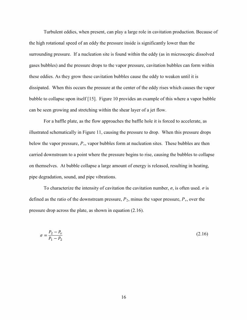
bubble to collapse upon itself [15]. Figure 10 provides an example of this where a vapor bubble
can be seen growing and stretching within the shear layer of a jet flow.
For a baffle plate, as the flow approaches the baffle hole it is forced to accelerate, as
illustrated schematically in Figure 11, causing the pressure to drop. When this pressure drops
below the vapor pressure, Pv
To characterize the intensity of cavitation the cavitation number, σ, is often used. σ is
defined as the ratio of the downstream pressure, P
, vapor bubbles form at nucleation sites. These bubbles are then
carried downstream to a point where the pressure begins to rise, causing the bubbles to collapse
on themselves. At bubble collapse a large amount of energy is released, resulting in heating,
pipe degradation, sound, and pipe vibrations.
2, minus the vapor pressure, Pv
(2.16)
, over the
pressure drop across the plate, as shown in equation .
𝜎𝜎 =𝑃𝑃2 − 𝑃𝑃𝑣𝑣𝑃𝑃1 − 𝑃𝑃2
(2.16)
17
Figure 10: Example of cavitation bubble formation within the shear layer from a baffle plate within a pipe section from [16].
A cavitation number based off of the upstream pressure is also often used as shown in
equation (2.17). These two cavitation numbers can be related by equation (2.18).
𝜎𝜎2 =𝑃𝑃1 − 𝑃𝑃𝑣𝑣𝑃𝑃1 − 𝑃𝑃2
(2.17)
𝜎𝜎 = 𝜎𝜎2 − 1 (2.18)
A cavitation number based off of the dynamic pressure rather than the pressure drop can
also be used and is defined in equation (2.19). σ and σv
(2.20)
can be related to each other, with the
pipe loss coefficient, as show in equation .

18
𝜎𝜎𝑣𝑣 =𝑃𝑃2 − 𝑃𝑃𝑣𝑣1/2𝜌𝜌𝑣𝑣𝑝𝑝2
(2.19)
𝜎𝜎 =𝜎𝜎𝑣𝑣𝐾𝐾𝐿𝐿𝑝𝑝
(2.20)
Figure 11: (Top) Illustration of the pressure variation across a sudden contraction and then sudden expansion. (Bottom) A schematic illustration of the vena-contracta section of a sudden contraction/sudden expansion (baffle plate) with reattachment of the flow occuring after the vena-contracta.

19
Because of the noise and vibrations that are produced when cavitation is occurring, These
two measures are often used to characterize cavitation levels [17]. Figure 12 shows the typical
behavior of the pipe wall acceleration as a function of cavitation number, σ, for a typical baffle
plate. Shown is the root mean square (RMS) of the pipe wall acceleration, A′, plotted with
respect to the cavitation number. The data reveal the existence of four distinct cavitation
regimes. The first (black line) is the turbulent regime where cavitation has not occurred and the
vibrations are due entirely to the turbulent jets. The second (red line) is where the acceleration
levels dramatically increase over a short span of cavitation numbers. This regime represents
where cavitation has onset, although the cavitation in this regime is only intermittent. The third
(blue line) is the regime where the flow is fully cavitating. The fourth (green line) is where
choking has occurred and the vibration levels decrease. The points where the lines intersect are
all critical cavitation numbers and are defined as [18]:
• The inception cavitation number (σ i
• The critical cavitation number (σ
)
c
• The choking cavitation number (σ
)
ch
The incipient cavitation number, σ
).
i
10
, is the point where cavitation first occurs and where
small vapor bubbles are formed irregularly [ ]. The noise sounds like light intermittent
popping that can barely be heard over the turbulent flow generated noise [18]. This point is a
design limit that is often used when no cavitation is desired within a system [18].
The critical cavitation number, σc
15
, is where the flow is fully cavitating, or there is a
constant generation of vapor bubbles [ ]. The noise that occurs at this point sounds like bacon
crackling [18]. This is a design limit that is used when some cavitation can be permitted. Many
systems that operate continuously are often run to this limit [18].

20
Figure 12: A representative plot of A’ vs. the cavitation number, σ, showing four different cavitation regimes. The black line is the non-cavitating regime, the red line is the incipient cavitation regime, the blue line is the fully cavitating regime, and the green line is the choked cavitating regime. The intersection of the red and black lines is the incipient cavitation design limit, σ i, the intersection of the blue and red lines is the critical cavitation design limit, σc. and the intersection of the green and blue lines is the chocked cavitation design limit , σch.
The choking cavitation number (σch
It has been shown that the cavitation number, although non-dimensional, is not free from
scaling effects like other non-dimensional numbers are. A scaling effect is when the changing of
size or pressure variations from application to application has effects on the parameter. This has
made it difficult to model cavitation. The cavitation number is affected by both size scale effects
and also pressure scale effects [
), which is not explored in this research, is the point
where choked flow, due to the amount of cavitation bubbles in the flow, is occurring. This is the
point when the flow has reached a maximum mass flow rate and can no longer increase with
increased pressure drop.
16]. Tullis stated, however, that in the cases of obtaining

21
inception and critical cavitation values the uses of pressure scale effects are not needed when
using an orifice plate or sudden enlargement [15].
The size scale effect that is currently used in industry is shown in equations (2.21)-(2.22).
[18,15,16] As can be seen, the size scale effect is dependent upon the pipe diameter, D, the
baffle hole diameter, d, and the pipe loss coefficient, KLp
15
. These equations are developed
empirically by studies conducted by Tullis with single hole orifice plates [ ].
𝑆𝑆𝑆𝑆𝑆𝑆 = �𝐷𝐷𝑑𝑑�𝑌𝑌
(2.21)
𝑌𝑌 = 0.25𝐾𝐾𝐿𝐿𝑃𝑃−0.3 (2.22)
As shown in equations (2.23)-(2.24) to obtain the adjusted cavitation inception and
critical number, σi* and σc
*, the actual cavitation number at inception, or critical value, (σ i and
σc) must be multiplied by the size scale effect, SSE, described above. σi* and σc
*
𝜎𝜎𝑖𝑖∗ = 𝑆𝑆𝑆𝑆𝑆𝑆𝜎𝜎𝑖𝑖
are cavitation
numbers adjusted for size scale effects.
(2.23)
𝜎𝜎𝑐𝑐∗ = 𝑆𝑆𝑆𝑆𝑆𝑆𝜎𝜎𝑐𝑐 (2.24)

22
2.4 Literature Review
The following discusses literature that defines the current state of turbulence and
cavitation induced pipe vibrations for liquid flow through baffle plates. They are divided into
two sections those describing turbulence induced vibrations and those addressing cavitation
induced vibrations.
2.4.1 Turbulent Induced Pipe Vibrations
In a study performed by Qing et. al. [19], wall pressure fluctuations caused by water flow
through single hole orifices were explored experimentally. Two orifices with through area ratios
of AH/Ap= 0.255 and 0.335 were used in the investigation with flow rates of 15, 20, 25 m3
Thompson [
/h. It
was shown that the majority of the pressure fluctuations occurred right after the orifice plate.
This was believed to be due to the large circulating flow that is produced outside of the shear
layer of the jet. The RMS of the pressure fluctuations and the peak frequency of the pressure
density, decreased with increased distance in the streamwise direction from the orifice plate. It
was also observed that the smaller the through area ratio the higher the RMS of the pressure
fluctuations were. The investigation also looked into the pipe vibrations that were occurring so as
to observe the strength of the fluid-structure interactions. The results revealed that the lower
frequency vibrations that occurred were at about the pipe natural frequencies showing that the
system was a weakly coupled fluid-structured system.
7] conducted a preliminary experimental investigation of baffle plate
influence on pipe vibrations. The experiments were conducted using five baffle plates of varying
baffle hole diameters ranging from 0.159 -2.54 cm with a pipe section that was 10.16 cm
diameter PVC pipe. The total through area ratio, AH/Ap, for all plates was nominally 0.438. Pipe
23
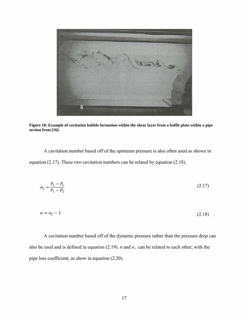
wall acceleration data were acquired over a range of average pipe fluid velocities ranging from
0-7 m/s. The root mean square (RMS) of the acceleration data were acquired, defined as A′, and
compared to the flow velocities and the streamwise distance from the baffle plate, x/D. The
investigation showed that the measured vibration levels within the turbulent regime increase with
increased baffle hole size, while holding AH/Ap
Figure 13
constant. It was also shown that the magnitude
of the vibration levels decreases with increasing distance downstream of the baffle plate
normalized by the pipe diameter, x/D, as illustrated in [7]. For the case of no baffle
plate, there is essentially no variation in the observed A′ level with change in measurement
location, x/D, on the pipe. When a baffle plate is present, however the vibration levels are
strongly dependent upon the measurement location. This result shows that at small x/D the
acceleration of the pipe is greater, as expected. With increasing x/D, the vibrations decay and
eventually merge with the no baffle plate levels. The location where the vibrations have
attenuated was observed to increase with increased baffle hole size.
Figure 13: Pipe wall acceleration vs. downstream distance normalized by the pipe diameter, x/D, for 5 baffle plates with varying hole diameters and a no baffle plate case as measured by Thompson as shown in the legend [7].

24
It was also shown that when a baffle plate was present, A′ scaled approximately with the
pipe fluid velocity to a power that varied with baffle hole size. This power approached the power
of two (for no baffle plate case) with decreased hole size [7].
2.4.2 Cavitation Induced Pipe Vibrations
A study was performed on noise generated from a single-hole orifice plate and one multi-
hole orifice plate by Testud et. al. [13]. The experiments conducted were in an open water loop
made of smooth steel pipe with an inner diameter of 7.4 cm and a pipe wall thickness of 0.8 cm.
Only two plates were tested, a single hole orifice plate with orifice diameter of 2.2 cm and
thickness of 1.4 cm, and a multi-hole orifice plate with plate thickness of 1.4 cm and 47 sharp-
edged holes of a diameter of 0.3 cm. The Reynolds number based on the average pipe fluid
velocity and pipe diameter varied from 2 x 10⁵ to 5 x 10⁵
Thompson [
. The results showed that cavitation
inception occurred at a cavitation number of σ ≅ 7.4 for both plates. It was observed that sound
levels were much higher for the single-hole orifice plate compared to the multi-hole plate with
the same through area ratio. Whistling was observed for the single-hole orifice plate only, and it
was concluded that the whistling phenomenon is a function of the plate thickness ratio. It was
also shown that the loss coefficient of the plate is a function of the plate thickness ratio and was
estimated using the Borda-Carnot model. In a comparison between cavitation noise from the
single hole orifice and standard turbulent noise from a non-cavitating plate there was good
agreement within the low frequency range.
7] performed a preliminary study on liquid flow through baffle plates, as was
discussed in section 2.1. Over the range of flow rates that were explored, for three of the five
25
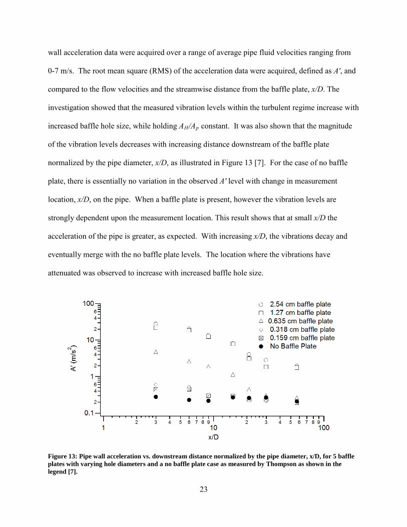
baffle plates that were employed cavitation was present. It was observed that by increasing the
size of the baffle plate holes, cavitation occurred at lower flow rates. This can be seen in Figure
14 [7], where cavitation was not seen to be present until the hole size was increased to 0.635 cm
at an average pipe fluid velocity of nominally 5.8 m/s. As the hole size was increased, cavitation
occurred at lower flow velocities and for the baffle plate with hole sizes of 2.54 cm cavitation
occurred at a flow rate of about 2.7 m/s. It was shown that the A′ level was about an order of
magnitude greater for flows where cavitation was present as compared to when it was not.
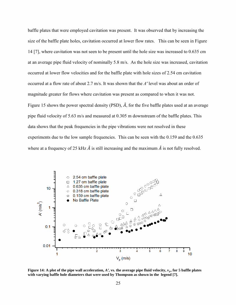
Figure 15 shows the power spectral density (PSD), �̂�𝐴, for the five baffle plates used at an average
pipe fluid velocity of 5.63 m/s and measured at 0.305 m downstream of the baffle plates. This
data shows that the peak frequencies in the pipe vibrations were not resolved in these
experiments due to the low sample frequencies. This can be seen with the 0.159 and the 0.635
where at a frequency of 25 kHz �̂�𝐴 is still increasing and the maximum �̂�𝐴 is not fully resolved.
Figure 14: A plot of the pipe wall acceleration, A′, vs. the average pipe fluid velocity, vp7
, for 5 baffle plates with varying baffle hole diameters that were used by Thompson as shown in the legend [ ].

26
Figure 15: Power spectral density, 𝑨𝑨�, vs. frequency, f, for five baffle plates with varying baffle hole diameters studied by Thompson [7], as shown in the legend, at a flow speed of 5.63 m/s measured at 0.305 m downstream from the baffle plate.
Tullis et. al. [9] conducted an experimental study on flow through perforated orifice
plates and discussed how they are used as energy dissipaters. The study was performed on six
plates, all of a thickness of 2.54 cm that varied in number of holes from 19-121 holes. The
perforated hole diameter for each plate was 2.54 cm with a large rounding radius of 0.95 cm for
the inlet of each hole. Flow through 25.4 cm, 40.64 cm, and 50.8 cm pipes was considered.
Through this study it was shown that the inception cavitation number, σi, for multi-hole orifice
plates is dependent upon the coefficient of discharge, cd (2.25), defined in equation . Figure 16
reveals the results of cavitation as a function of the discharge coefficient. The data shows that
with decreased discharge coefficient the onset of cavitation occurs at lower cavitation numbers.
The study also revealed that the suppression of cavitation, caused by the interacting jets, is
lessened with decreased pipe size. It was believed that with a small enough pipe diameter the

27
flow would behave like a single hole orifice plate. Through the entire flow regime that was
investigated, no cavitation erosion damage was observed on the pipe wall for any of the orifice
plates used.
𝑐𝑐𝑑𝑑 =𝑣𝑣𝑝𝑝
�2(𝑃𝑃1−𝑃𝑃2)𝜌𝜌
+ 𝑣𝑣𝑝𝑝2 (2.25)
Figure 16: A plot of inception cavitation number vs. discharge coefficient for 4 multi-hole orifice plates used by Tullis et. al. [9]
2.5 Current State of the Art
The current state on cavitation and turbulent induced vibrations caused by baffle plates is
limited in understanding and is summarized as follows:

28
• Characterization of cavitation inception for baffle plates is limited to the study
done by Tullis et. al. [9] which was incomplete in that it did not investigate the
effects of hole diameter and plate thickness and only considered rounded holes.
• The exploration of cavitation inception for sharp edged baffle plates has not been
explored by any previous study to the author’s knowledge.
• The characterization of A′ levels for turbulent induced vibrations for baffle plate
induced turbulent jets is limited and the influence of plate thickness and through
area ratio has not been explored, parametrically.
• The characterization of the attenuation of A′ level with downstream distance is
limited to the study done by Thompson [7]. However in his study the pipe length
and scenarios considered were insufficient to obtain robust results in the
cavitation regime.
• Models for predicting the loss coefficient is restricted to the Borda-Carnot model
explained in section 2.2 and does not adequately account for variation in the
baffle plate thickness.
• No robust models for prediction of cavitation inception for baffle plates have been
produced due to lack of experiments performed.
2.6 Research Contributions
This work explores experimentally the effects of turbulent and cavitation induced
vibrations. This work investigates the dependences of the problem over a larger range of the
expected variables than the current state of the art. A total of sixteen sharp edged baffle plates

29
were used with through area ratios ranging from 0.109-0.609, hole diameters ranging from 0.159
cm-2.54 cm, thickness ratios ranging from 0.32-0.64, and average pipe fluid velocities ranging
from 0.35-8.5 m/s. This large parameter range allows for characterization to the influence of
baffle plate thickness, baffle hole diameter, and number of baffle holes. Further, empirical
models for predicting inception and critical cavitation have been produced. In addition, empirical
models for predicting A′ levels as a function of the influencing variables have also been
developed.

30

31
3 EXPERIMENT SETUP
The test facilities that were used to conduct all experiments consisted of the same large
water flow loop that was used by Thompson [7]. A total of 16 baffle plates (shown in Figure 21)
were used with varying baffle hole diameters, through area ratios, and plate thickness. The
following sections give a detailed description and explanation of each section of the flow loop.
A description of the baffle plates that were used is also provided. Lastly, a discussion of the
instrumentation that was used to obtain measurements will be discussed.
3.1 Flow Loop
Shown in Figure 17 is a schematic drawing of the flow loop facility. A photograph of a
portion of the flow loop is shown in Figure 18. Flow is delivered by a Bell and Gossett
centrifugal pump, driven by a 75 hp Marathon Electric 365T motor shown in Figure 18. The
inlet and outlet pipes to the pump are 20.3 cm and 10.2 cm Schedule 80 PVC pipe. Downstream
of the pump is a flow conditioner within an expanded pipe of 20.32 cm diameter Schedule 80
PVC pipe. This can also be seen in Figure 18. The flow conditioner consists of a 7.6 cm thick
piece of aluminum honeycomb and three mesh screens all held together by aluminum rings to
keep it from being forced downstream. The flow conditioner is used to straighten the flow and
eliminate eddies formed by the pump. Following the flow conditioner is a reducer to 10.2 cm
Schedule 80 pipe. After the reduction a Proco Series 310 rubber coupler is mounted. This is

32
Figure 17: Schematic drawing of the flow loop facility used for all experiments.
Figure 18: Photograph of the centrifugal pump and flow conditioner used in flow loop facility. Downstream of the flow conditioner the rubber coupler and developing region can be seen.
6.1 m 6.1 m 6.1 m 3.04 m
2.1 m

33
used to reduce the upstream structural vibrations caused by the pump and the flow through the
pipe bends. The pipe is mounted to the wall both before and after the rubber coupler to also
reduce the structural vibrations. After the rubber coupler is the developing region of the flow
loop which allows the flow to become fully developed before the test section, or region where
measurements are acquired. The developing region consists of a 6.1 m long 10.2 cm diameter
Schedule 80 PVC pipe. Using the Schlichting-Gersten equation [12], shown in equation (3.1),
the length of the pipe was verified to be long enough to allow for fully developed flow. The, 𝑙𝑙𝑒𝑒 ,
is the length of the developing section, D, is the pipe diameter, and, ReD
𝑙𝑙𝑒𝑒𝐷𝐷≈ 4.4𝑅𝑅𝑒𝑒𝐷𝐷
1/6
, is the Reynolds number
based upon the pipe Diameter.
(3.1)
Connected to the developing region is the pipe test section, which is made up of two 6.1
m long, 10.16 cm diameter schedule 40 PVC pipes. A photograph of the test section is shown in
Figure 19. The baffle plates, as shown and discussed in section 3.2, are inserted between the test
section and the developing region, as shown in Figure 20. Following the test section, the pipe
eventually bends 180o and connects to a control valve that is used to release the water from the
flow loop if needed. Following the valve is a section of transparent pipe. This is used to visually
inspect the flow for air bubbles. A vertical chimney vent that extends above the elevation of the
entire flow loop is located after the transparent pipe. This chimney is used to fill the flow loop
and also allows all the air in the system to escape. A Proco Series 310 rubber coupler follows the
chimney vent and connects to an expansion that increases the pipe diameter to 20.32 cm before
the pipe connects to the inlet of the pump.

34
Figure 19: Photograph of the pipe test section showing the location of the thermocouple and flow meter relative to the test section.
Figure 20: Photograph of a baffle plate mounted between the developing region and test section. The locations of the upstream and downstream pressure transducers along with microphone and accelerometer are also shown.

35
3.2 Baffle Plates
All baffle plates were made of aluminum and had a diameter of 22.9 cm. The baffle
plates have nominal hole diameters of 2.54 cm, 1.27 cm, 0.64 cm, 0.32 cm, and 0.16 cm. All
baffle plates exhibited sharp edge holes except the 0.16 cm diameter hole with 896 holes. The
percent openness of each baffle plate was nominally 10.9%, 21.9%, 43.8%, and 60.9%. The
thicknesses of the plates were nominally 0.31 cm, 0.51 cm, or 0.65 cm. Table 1 provides a
detailed list of the baffle plates employed and their associated characteristics. Figure 21 shows
an image of each of the baffle plates.
Table 1: Baffle plates used in the study with baffle hole diameter, number of baffle holes, and baffle plate thickness shown.
Plate Label
Baffle Hole Diameter
(cm)
Baffle Plate Thickness
(cm)
Number of Baffle Holes
Through Area Ratio
AH/ApA1
2.53 0.66 7 0.434
A2 2.54 0.65 4 0.211 B1 1.27 0.66 28 0.435 B2 1.26 0.66 14 0.217 B3 1.27 0.31 7 0.109 B4 1.27 0.64 7 0.109 C1 0.64 0.65 156 0.611 C2 0.64 0.67 112 0.438 C3 0.65 0.65 57 0.233 C4 0.63 0.65 28 0.109 D1 0.32 0.51 624 0.607 D2 0.32 0.51 448 0.451 D3 0.32 0.56 224 0.225 D4 0.31 0.52 112 0.108 E1 0.16 0.50 1793 0.435 E2 0.16 0.54 896 0.220

36
Figure 21: Photographs of the sixteen baffle plates used in the study, showing arranged in the same order as Table 1 from left to right and top to bottom.
3.3 Instrumentation
A single PCB Piezotronics ICP 352C68 accelerometer was used to measure the pipe wall
acceleration. The sensitivity of the accelerometer was 10.2 mV/( m/s2), the range was +/- 491
m/s2, and the resolution was 1.5 x 10⁻³ m/s2. The accelerometer was placed on the side of the
A1 A2 B1 B2
B3 B4 C2 C1
C3 C4 D1 D2
D4 D3 E1 E2

37
pipe test section three diameters downstream, for the experiment used to characterize cavitation
inception and vibrations; and from three to 110 diameters downstream of the of the baffle plate,
for the experiment used to characterize the attenuation of vibrations. An LD 2551 microphone
and PRM 426 preamp having a sensitivity of 50 mV/Pa, with a range up to 139 dB, were used to
measure sound levels. The microphone was placed three diameters downstream of the baffle
plate on the side of the pipe opposite of the accelerometer.
Two Omega PX 309 static pressure transducers with ranges from 0-100 psi, and accuracy
of +/- 0.25%, were placed three diameters upstream and six diameters downstream of the baffle
plate. The pressure transducers were used to measure the pressure drop across the baffle plate.
Downstream of the pipe test section, an Omega FP6500 series paddlewheel with a range
of 0.1-9m/s and accuracy of ±1.5%, was used to measure the flow rate in the test section. Also
downstream of the test section a K-type thermocouple with accuracy of ±0.05 oC was used to
measure the fluid temperature so as to determine the vapor pressure and water properties.

38

39
4 EXPERIMENTAL PROCEDURES
Two types of experiments were performed in this research. The first were experiments
that characterized cavitation inception and pipe vibrations immediately downstream of the baffle
plates. The second were experiments conducted to characterize the attenuation of pipe vibrations
with streamwise distance. The following will discuss the measurements conducted by each
experiment, followed by a discussion of the data analysis. Lastly, a section addressing the
uncertainty analysis is provided.
4.1 Measurements of Cavitation Inception and Pipe Vibrations
Experiments were conducted in the cavitating and non-cavitating regimes to characterize
the initiation of cavitation and the pipe wall acceleration over a range of average pipe fluid
velocities from 0.35-8.5 m/s. An accelerometer and microphone were placed three diameters
downstream of the baffle plate. These were used to measure the pipe wall acceleration and sound
levels emitted from the pipe. Two pressure transducers were placed respectfully two and six
diameters upstream and downstream of the baffle plate to measure the static pressure drop across
the baffle plate, P1-P2
Figure 17
. A paddle wheel was placed far downstream of the pipe test section to
measure the bulk fluid flow rate. A thermocouple was placed downstream of the test section to
measure the fluid temperature. The location of these instruments can be seen in -Figure
20.

40
The accelerometer, pressure, noise, and flow rate data were acquired at a sample rate of
50 kHz for 5 seconds for each pipe velocity considered. A 2 Hz high pass filter and a 20 kHz
low pass filter were used to filter the acceleration and microphone data. The filters were used to
filter the low frequency noise that was occurring due to low frequency pipe swaying at the lower
end and the resonant frequencies of the measurement devices at the high frequencies. These
measurements were acquired for each of the 16 baffle plates over as large of flow speed as
possible for each plate. Two independent tests were conducted for every scenario and the results
were averaged. Table 2 shows the maximum variation of all the scenarios of σ, σv, vH, and KLp
Table 2: The maximum variation in the two different independent tests that were conducted
for every scenario for the variables that was determined at both incipient and critical
cavitation as seen below.
at incipient and critical cavitation between the two independent tests that were conducted.
Incipient Cavitation
Critical Cavitation
σ 6.8% v 4.4% σ 4.0% 10.0% v 4.6% H 4.8% K 7.5% Lp 5.7%
4.2 Data Analysis of Cavitation and Pipe Vibrations
The measurement data collected, as described in section 4.1, were post-processed to
obtain the RMS of the sound and acceleration data (A′ and S′) for each velocity measurement.
The time averages of the pressure and flow rate measurements were also acquired for each
velocity measurement.
41
To obtain the cavitation numbers, average baffle fluid velocity, A′, and the loss
coefficients at the incipient and critical points, the process that was discussed in section 2.3 and
shown in Figure 12 was used and will be described here.
To determine the point of cavitation inception and critical cavitation, the rms of pipe wall
acceleration, A′, was plotted as a function of σ, σv, and vH (4.6). Where σ is defined in equation ,
σv (4.10)is defined in equation , and vH
𝜎𝜎 =𝑃𝑃2 − 𝑃𝑃𝑣𝑣𝑃𝑃1 − 𝑃𝑃2
is the baffle hole velocity.
(4.1)
𝜎𝜎𝑣𝑣 =𝑃𝑃2 − 𝑃𝑃𝑣𝑣1/2𝜌𝜌𝑣𝑣𝑝𝑝2
(4.2)
The natural logarithm of each variable was determined and the data were plotted, as illustrated
for each variable in Figure 22-Figure 24. Figure 22- Figure 24 are plots that show A’ versus σ,
σv, or vH
2.3
. From plots of these nature the incipient and critical cavitation points can be
determined. To do this a linear regression analysis (y=mx+b) was performed for each of the
three linear sections of data evident in the figures, these linear sections correspond to the non-
cavitating, incipient and fully cavitating regimes as discussed in section and shown in Figure
12. The points of intersection of the three linear sections were determined to be the points of
cavitation inception and critical cavitation. This method was performed for each of the two sets
of data obtained for each baffle plate and the results were averaged.
The plate loss coefficient based off the average pipe velocity, KLp
(4.3)
, (defined in equation
) was calculated at the incipient cavitation design limit using equation (4.4). σi is the

42
incipient cavitation number and σvi
(4.5)
is also an incipient cavitation number but based off of the
dynamic pressure and is defined in equation .
𝐾𝐾𝐿𝐿𝑝𝑝 =𝑃𝑃1 − 𝑃𝑃2
1/2𝜌𝜌𝑣𝑣𝑝𝑝2 (4.3)
𝐾𝐾𝐿𝐿𝑝𝑝 =𝜎𝜎𝑣𝑣𝑖𝑖𝜎𝜎𝑖𝑖
(4.4)
𝜎𝜎𝑣𝑣 =𝑃𝑃2 − 𝑃𝑃𝑣𝑣1/2𝜌𝜌𝑣𝑣𝑝𝑝𝑖𝑖2 (4.5)
Figure 22: Ln(A′) vs. Ln(vH) used to obtain inception and critical cavitation values. Values of the coefficients m and b for the linear form y=mx+b are shown for each of the three linear regimes.

43
Figure 23: Ln(A′) vs. Ln(σ) used to obtain inception and critical cavitation values. Values of the coefficients m and b for the linear form y=mx+b are shown for each of the three linear regimes.
Figure 24: Ln(A′) vs. Ln(σv
) used to obtain inception and critical cavitation values. Values of the coefficients m and b for the linear form y=mx+b are shown for each of the three linear regimes.
44
The inception and critical cavitation number were normalized by the size scale effect
discussed in section 2.3 and were compared to the discharge coefficient as was done by Tullis
[9]. The A′ values at inception and critical cavitation were also normalized as shown in equation
(4.6), where again d is the baffle hole diameter and vH is the baffle hole velocity. The non-
dimensionalized A′, A′*, was compared to the thickness to baffle hole diameter, t/d, the through
area ratio, AH/Ap
𝐴𝐴′ ∗ =𝐴𝐴′𝑑𝑑𝑣𝑣𝐻𝐻2
, and the cavitation number, σ. Empirical models were then developed for the
cavitation number and A′, at the points of inception and critical cavitation.
(4.6)
The loss coefficient based on the baffle hole velocity (KLH (4.7)), as shown in equation
and can be calculated from KLp (4.3) as shown in equation and is determined from equation (4.8),
was normalized by the theoretical attached loss coefficient model as was developed in 2.2.2 and
shown in equation (4.9). This ratio (KL/KLA) was then evaluated as a function of the plate
thickness to diameter ratio, t/d, and the through area ratio, AH/Ap
𝐾𝐾𝐿𝐿𝐻𝐻 =𝑃𝑃1 − 𝑃𝑃2
1/2𝜌𝜌𝑣𝑣𝐻𝐻2
. An empirical model to predict
the loss coefficient based upon geometric variables was then developed.
(4.7)
𝐾𝐾𝐿𝐿𝐻𝐻 = 𝐾𝐾𝐿𝐿𝑝𝑝 �𝐴𝐴𝐻𝐻𝐴𝐴𝑝𝑝�
2
(4.8)

45
𝐾𝐾𝐿𝐿𝐴𝐴 = �1 − 2 �𝐴𝐴𝑝𝑝𝐴𝐴𝐻𝐻� + 2 �
𝐴𝐴𝑝𝑝𝐴𝐴𝐻𝐻�
2
�1 −1𝛼𝛼
+1
2𝛼𝛼2���𝐴𝐴𝐻𝐻𝐴𝐴𝑝𝑝�
2
(4.9)
4.3 Measurements of Attenuation of Pipe Vibrations
Experiments were also conducted in both the cavitating and non-cavitating regimes to
characterize the attenuation downstream of the baffle plates. A total of 14 baffle plates were
tested for this part of the study. Due to the limitations on length of pipe, two 6.1 m long, 10.16
cm diameter, pipes were flanged together to make up the entire test section.
Accelerometers were mounted on the wall of the pipe at locations ranging from 3-110
diameters downstream, x/D, of the baffle plate. The pressure drop across the baffle plate was
measured using two pressure transducers that were placed three and six diameters up and
downstream of the baffle plate. A paddle wheel was placed far downstream of the pipe test
section to measure the liquid flow rate.
The pipe wall acceleration (at 26 x/D locations from 3-110), pressure drop, and average
pipe fluid velocity measurements were taken for 2-4 average pipe velocities ranging from 0.6-6.6
m/s. The variation of velocity measurement was to allow for measurements in both non-
cavitating and cavitating regimes. The data were collected at a sample rate of 50 kHz for 5
seconds for each pipe velocity measurement and x/D location. A 2 Hz high pass filter and a 20
kHz low pass filter were used to filter the acceleration and microphone data. The filters were
used to filter the low frequency noise that was occurring due to pipe swaying and the resonant
frequencies of the measurement devices.

46
4.4 Data Analysis of Attenuation of Pipe Vibrations
The attenuation measurement data were post-processed to obtain the RMS of the
acceleration data (A′) for each velocity measurement. The time averages of the flow rate
measurements were also taken for each velocity measurement.
A non-dimensionalized A’ value, 𝐴𝐴2′∗, as shown in equation (4.10), was plotted versus x/D
and a double exponential form of a curve fitting function was applied to the data. When the
value 𝐴𝐴2′∗ decreased to 1.5 times the no baffle plate value of 𝐴𝐴2
′∗ this point was determined to be
the point when the vibrations had attenuated or decayed.
𝐴𝐴2′∗ =
𝐴𝐴′𝐷𝐷𝑣𝑣𝑝𝑝2
(4.10)
Figure 25 illustrates 𝐴𝐴2′∗ versus x/D for a representative baffle plate at four different
velocities. From plots of this nature the point of attenuation of vibrations can be illustrated. The
x markings show the attenuation point for these curves, determined by 𝐴𝐴2′∗ reaching 1.5 times the
no baffle plate 𝐴𝐴2′∗. As can be seen at a x/D = 3 the vibrations decreases to an asymptotic value,
which is the non-baffle plate vibration levels.
4.5 Uncertainty Analysis
Uncertainties in the measurements and variables described in section 4.3 are now
discussed. Several sources of uncertainty exists which include the uncertainty in the regression
analysis (to find σi, σc, σvi, σvc, vHi, and vHc), in the calculation of KLp, AH/Ap, and t/d and the
measurements taken. First the uncertainty in the regression analysis to find σi, σc, σvi, σvc, vHi,

47
and vHc will be discussed. The measurement uncertainty will then be discussed. Concluding this
section will be a discussion of the uncertainty in the calculation of KLp, AH/Ap
, and t/d.
Figure 25: A representative plot of 𝑨𝑨𝟐𝟐′∗ vs. x/D for four different baffle hole velocities for one baffle plate. The x markings indicate 1.5 time the no baffle plate vibrations.
4.5.1 Regression Analysis Uncertainty
The uncertainty of the points, σi, σc, σvi, σvc, vHi, and vHc
4.2
, obtained from the regression
analysis (discussed in section ) is calculated from equation (4.11) [20]. This is the error
associated with the x-axis variable (being σi, σc, σvi, σvc, vHi, or vHc
20
) that was used to create the
regression line, where 𝑋𝑋� is the regression value for a given A′ value and X is the measured value
at that point. The i and j’s represent the two different lines used to find the intersecting point. The
variables N and M are the respected number of data points used in the regression analysis for
each line [ ]. The number of data points is subtracted by two because there are two constants
that were used to produce the regression line, m and b (mx+b).

48
𝜌𝜌𝑥𝑥 = ±�∑ �𝑋𝑋𝑖𝑖 − 𝑋𝑋�𝑖𝑖�
2𝑁𝑁𝑖𝑖=1𝑁𝑁 − 2
+∑ �𝑋𝑋𝑗𝑗 − 𝑋𝑋�𝑗𝑗 �
2𝑀𝑀𝑗𝑗=1
𝑀𝑀 − 2
(4.11)
Table 3 shows the uncertainty determined using the above method for the cavitation
numbers and baffle hole fluid velocity at incipient and critical cavitation. This lists the
maximum, minimum, and average uncertainties calculated. This shows that from the regression
analysis all uncertainties are below 25%, where all the average uncertainties of all the variables
are below 12%.
Table 3: Uncertainty in determining design limits
Average Incipient
Cavitation
Min. Incipient
Cavitation
Max. Incipient
Cavitation
Average Critical
Cavitation
Min. Critical
Cavitation
Max. Critical
Cavitation v 3.6% H 2% 8.3% 1.9% 1% 2.5% σ 10.4% 5.3% 18.4% 3.3% 1.6% 6.2% σ 11.1% v 5.3% 22.3% 3.4% 2.4% 4.8%
4.5.2 Measurement Uncertainty
Measurements were acquired for the pressure, pipe wall acceleration, flow rate,
temperature, plate thickness, and baffle hole diameter. Each of these measurements had
uncertainty associated with it cause by the accuracy of the measurement devices. The uncertainty
in the pressure measurements was limited to the instrument accuracy of ±0.25%. The accuracy
of the accelerometer was ±7.5 x 10⁻⁴ m/s2. The baffle hole diameter and plate thickness

49
uncertainty was ±5 x 10⁻⁵ m. The Uncertainty of the thermocouple was ±5 x 10⁻² o
4.5.3 Calculated Variables Uncertainty
C. The
uncertainty of the flow meter was ±1.5%.
The uncertainty in a calculated variable R is a function of the uncertainty of the variables
that R is a function of as can be seen in equations (4.12) and (4.13), where uR is the uncertainty
of R and ux 21 is the uncertainty of x [ ]. To find the total uncertainty in R, equations (4.14) and
(4.15) where used [21]. This method was used in finding the overall uncertainty of KLp, AH/Ap
𝑅𝑅 = 𝑓𝑓(𝑥𝑥1,𝑥𝑥2, … , 𝑥𝑥𝐿𝐿)
,
and t/d and will be discussed below.
(4.12)
𝜌𝜌𝑅𝑅 = 𝑓𝑓(𝜌𝜌𝑥𝑥1 ,𝜌𝜌𝑥𝑥2 , … ,𝜌𝜌𝑥𝑥𝐿𝐿) (4.13)
𝜃𝜃𝑖𝑖 =𝜕𝜕𝑅𝑅𝜕𝜕𝑥𝑥𝑖𝑖
𝑖𝑖 = 1,2, … , 𝐿𝐿 (4.14)
𝜌𝜌𝑅𝑅 = ±���𝜃𝜃𝑖𝑖𝜌𝜌𝑥𝑥𝑖𝑖�2
𝐿𝐿
𝑖𝑖=1
(4.15)

50
The value of KLp is a function of P1, P2, vp (4.16), and ρ as shown in equation . Using
both equation (4.14) and (4.15) an equation for finding 𝜌𝜌𝐾𝐾𝐿𝐿𝑝𝑝 R can be obtained and is shown in
equation (4.17). Note that in equation (4.17) there is an additional term uE. This is the standard
deviation of KLp for the non-cavitating regime. This was an average of ±2.4% for all the baffle
plates. The total uncertainty of KL
𝐾𝐾𝐿𝐿𝑝𝑝 =𝑃𝑃1 − 𝑃𝑃2
1/2𝜌𝜌𝑣𝑣𝑝𝑝2
was an average of ±4.1% for all the baffle plates used with a
maximum and minimum uncertainty of ±5.6% and ±3.3%.
(4.16)
𝜌𝜌𝐾𝐾𝐿𝐿𝑝𝑝 = ±��𝜕𝜕𝐾𝐾𝐿𝐿𝑝𝑝𝜕𝜕𝑃𝑃1
𝜌𝜌𝑃𝑃1�2
+ �𝜕𝜕𝐾𝐾𝐿𝐿𝑝𝑝𝜕𝜕𝑃𝑃2
𝜌𝜌𝑃𝑃2�2
+ �𝜕𝜕𝐾𝐾𝐿𝐿𝑝𝑝𝜕𝜕𝑣𝑣𝑝𝑝
𝜌𝜌𝑣𝑣𝑝𝑝 �2
+ �𝜕𝜕𝐾𝐾𝐿𝐿𝑝𝑝𝜕𝜕𝜌𝜌
𝜌𝜌𝜌𝜌�2
+ 𝜌𝜌𝑆𝑆2
= ±2�𝜌𝜌𝑃𝑃1
𝜌𝜌2𝑣𝑣𝑝𝑝4+
𝜌𝜌𝑃𝑃2
𝜌𝜌2𝑣𝑣𝑝𝑝4+ �
2(𝑃𝑃1 − 𝑃𝑃2)𝜌𝜌𝑣𝑣𝑝𝑝𝜌𝜌 𝑣𝑣𝑝𝑝3
�2
+ �(𝑃𝑃1 − 𝑃𝑃2)𝜌𝜌𝜌𝜌
𝜌𝜌2 𝑣𝑣𝑝𝑝2�
2
+ 𝜌𝜌𝑆𝑆2
(4.17)
The uncertainty of AH/Ap
(4.14)
is a function of the uncertainty of the baffle hole diameter, d,
and the diameter of the pipe, D. Using both equations and (4.15) an equation for finding
𝜌𝜌𝐴𝐴𝐻𝐻/𝐴𝐴𝑝𝑝 R can be obtained and is shown in equation (4.18). The average uncertainty of all the
baffle plates for AH/Ap
𝜌𝜌𝐴𝐴𝐻𝐻/𝐴𝐴𝑝𝑝 = ±��𝜕𝜕 𝐴𝐴𝐻𝐻𝐴𝐴𝑝𝑝
𝜕𝜕𝑑𝑑𝜌𝜌𝑑𝑑�
2
+ �𝜕𝜕 𝐴𝐴𝐻𝐻𝐴𝐴𝑝𝑝
𝜕𝜕𝐷𝐷𝜌𝜌𝐷𝐷�
2
= ±2��𝑑𝑑𝑛𝑛𝜌𝜌𝑑𝑑𝐷𝐷2 �
2
+ �𝑑𝑑2𝑛𝑛𝜌𝜌𝐷𝐷𝐷𝐷3 �
2
is about ±0.1%.
(4.18)
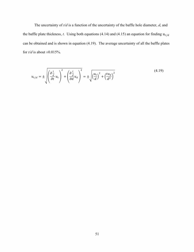
51
The uncertainty of t/d
(4.14)
is a function of the uncertainty of the baffle hole diameter, d, and
the baffle plate thickness, t. Using both equations and (4.15) an equation for finding 𝜌𝜌𝑡𝑡/𝑑𝑑
can be obtained and is shown in equation (4.19). The average uncertainty of all the baffle plates
for t/d is about ±0.015%.
𝜌𝜌𝑡𝑡/𝑑𝑑 = ±��𝜕𝜕 𝑡𝑡𝑑𝑑
𝜕𝜕𝑡𝑡
𝜌𝜌𝑡𝑡�
2
+ �𝜕𝜕 𝑡𝑡𝑑𝑑
𝜕𝜕𝑑𝑑𝜌𝜌𝑑𝑑�
2
= ±��𝜌𝜌𝑡𝑡𝑑𝑑�
2+ �
𝑡𝑡𝜌𝜌𝑑𝑑𝑑𝑑2 �
2
(4.19)

52

53
5 CHARACTERIZED RESULTS
This chapter discusses the characterized results of the experiments that were performed and
discussed in chapter 4. The results are divided into four sections. The first three sections will
discuss the general trends that occur due to the influencing variables. Specifically, these sections
will address the loss coefficient, cavitation inception, A′ levels, and attenuation of vibrations.
The last section provides a summary of the results that are presented in the previous sections.
5.1 Baffle Loss Coefficient
The loss coefficient is a significant variable when considering cavitation and flow
induced pipe vibrations. This is because the loss of pressure across a baffle plate is due to
energy being converted into other forms. These other forms of energy are thermal, acoustical,
internal (change of phase, from liquid to vapor for cavitation), and kinetic energy of the pipe wall
(vibrations). For this reason the baffle plate loss coefficient was explored in this work and the
results are discussed below.
Plotted in Figure 26 is the loss coefficient, KLH, versus the through area ratio (openness)
for the 16 baffle plates utilized. Data from Testud et. al. [13] are also shown for comparison.
Also plotted are two theoretical models that were developed from an integral analysis of a
sudden contraction followed by a sudden expansion as presented in section 2.2. The KLH data
shown corresponds to a flow velocity just prior to the point of cavitation inception, although KLH

54
is nominally constant prior this point. The two baffle plates that had through area ratios, AH/Ap =
60.9% (C4 and D4 in Table 1) did not cavitate at any speed so the KLH values for these plates
correspond to the maximum flow rate measured. KLA was discussed in section 2.2.2 and is given
again in equation (5.1). This is a model that assumes that the baffle plate is thick enough for the
flow to reattach after the formation of the vena-contracta. KLD was discussed in section 2.2.1 and
is given again in equation (5.2). It is based on a model that assumes the baffle plate is thin so that
the flow does not reattach. It can be seen from Figure 26 that the data follow the trends of the
two models and are bound by them as was expected. α is a the ratio of the jet from the vena-
contracta, vj, over the baffle hole velocity, vH. For KLA, α = 0.72 and for KLD, α = 0.61. The
value 0.61 is the theoretical value for a sharp edge orifice for a gas to a free space exit [13]. For
a sudden contraction area the α value varies from 0.62 to a value of 1, which would be valid for a
thick plate. The value of 0.72 was selected due to it being the best fit to the lower limit of the
data.
𝐾𝐾𝐿𝐿𝐴𝐴 = �1 − 2 �𝐴𝐴𝑝𝑝𝐴𝐴𝐻𝐻� + 2 �
𝐴𝐴𝑝𝑝𝐴𝐴𝐻𝐻�
2
�1 −1𝛼𝛼
+1
2𝛼𝛼2���𝐴𝐴𝐻𝐻𝐴𝐴𝑝𝑝�
2
(5.1)
𝐾𝐾𝐿𝐿𝐷𝐷 = ��𝐴𝐴𝑝𝑝𝐴𝐴𝐻𝐻�
1𝛼𝛼
− 1�2
�𝐴𝐴𝐻𝐻𝐴𝐴𝑝𝑝�
2
(5.2)
The spread between the two models is further illustrated in Figure 27 where KLH as a
function of the thickness to baffle hole diameter ratio, t/d, is shown. This data shows that for a
given through area ratio, KLH decreases with increased t/d until t/d ≈ 1.5-2.0 where KLH then
slightly increases with increasing t/d. The large decrease of KLH in the t/d < 1 range illustrates

55
that the loss coefficient is approaching the theoretical thick plate model and this shows that with
baffle plates of t/d ratios greater than one the theoretical thick plate model accurately predicts the
loss coefficient. The slight increase in KLH above t/d=1.5-2.0 is believed to be due to frictional
losses within the baffle holes.
Figure 26: Loss coefficient, KLH, vs. the total through area ratio, AH/Ap, for 16 baffle plates. Included is a theoretical attached model, KLA, and a theoretical detached model, KLD. Data from Testud et. al. is also included for comparison.
The two figures together show that the loss coefficient is dependent upon the through
area ratio as was expected but also upon the ratio of thickness of the baffle plate to the diameter
of the baffle hole. It also shows that the two theoretical models are only accurate for a range of
plate thicknesses. It is also worth noting that by holding AH/Ap constant, the plates with larger t/d
ratios exhibit a larger numbers of baffle holes. This fact illustrates that increased number of
baffle holes causes a suppression of the pressure loss that is occurring even when the total flow
area remains constant.

56
Figure 27: Loss coefficient, KLH, vs. the thickness ratio, t/d, for 16 baffle plates and four area ratios as shown in the legend.
5.2 Characterization of Vibrations and Incipient Cavitation
Figure 28 provides a representative plot of the pipe wall acceleration, characterized by A′,
versus the average baffle hole velocity for five different baffle plates with varying thickness to
diameter ratios, t/d, and a fixed through area ratio of nominally 43.8%. These measurements of
acceleration were obtained at three pipe diameters downstream from the baffle plate. It can be
seen that from this figure that each baffle plate has similar trends. The A′ levels gradually
increase in a power-law form with the baffle hole velocity, vH, until a definite change in slope
occurs. This initial regime is where the flow is non-cavitating and the pipe wall vibration is
caused by the turbulence in the flow. The slopes of these lines are similar for all baffle plates.
From the first influx point the A′ levels increase dramatically with increasing vH until a second
inflection point occurs. This essentially linear region is when the flow is starting to cavitate.
The amount of cavitation increases with vH causing A′ to also increase. From the second

57
inflection point and above, the flow is fully cavitating and the A′ levels again increase gradually
with a power-law dependence on vH. The slope in this region is similar for all baffle plates.
The two inflection points observed in the data correspond to the inception and critical
cavitation values. The data of Figure 28 also reveals that in general the A′ level increases with
decreasing t/d, both within the turbulent regime and the cavitating regime. It is also observed
that cavitation inception also occurs at higher average baffle hole velocities with increased t/d.
The velocity at cavitation inception for t/d=0.25 is about an order of magnitude greater than the
velocity at inception for t/d=3.3.
Figure 29 is a plot of A′ versus the average baffle hole velocity for 5 different thickness to
diameter ratios, t/d, and a fixed through area ratio, AH/Ap, of nominally 21.9%. The slight
variation in AH/Ap is due to it being impossible to create plates of constant AH/Ap for small
numbers of baffle holes. The data of this figure reveals that for increasing in t/d, the A′ levels
decrease and that cavitation inception occurs at higher velocities.
Comparing the results of both Figure 28 and Figure 29 to that of the previous section
which addressed the loss coefficient reveals that decreasing t/d yields increases in both the loss
coefficient and the A′. Thus, the A′ levels and the loss coefficient show similar dependence on
the flow and geometric variables. The added loss that occurs at smaller t/d results in enhanced
energy transfer to the pipe wall in the form of vibrations. Cavitation is also suppressed with
increasing t/d such that the inception point is shifted to higher velocities by nominally 48%
between smallest and largest t/d. Again, this can be attributed to these plates having lower loss
coefficients which result in smaller pressure drops.

58
Figure 28: A′ vs. average baffle hole velocity, vH, for five baffle plates of constant through area (AH/Ap=0.438) and five different t/d ratios as shown in the legend.
Figure 29: A′ vs. average baffle hole velocity, vH, for five baffle plates of nominally constant through area (AH/Ap=0.219) and five different t/d ratios as shown in the legend.

59
Figure 30 provides a representative plot of A′ versus the average baffle hole velocity for
four different baffle plates through area ratios of AH/Ap = 10.9, 21.9, 43.8, and 60.9%, and at a
fixed thickness to diameter ratio of t/d = 1.7. These data show that the vibration levels increase
with decreased through area ratio, and this is most pronounced in the cavitation regime. Between
the smallest to largest through area ratio the vibration levels have an order of magnitude
difference. It is also shown that cavitation inception occurs at higher velocities with increased
through area ratios to where cavitation occurs at a velocity nominally 18% higher for AH/Ap =
43.8% compared to AH/Ap = 10.9% . The AH/Ap = 60.9% baffle plate was never observed to
experience cavitation.
Figure 30: A′ vs. average baffle hole velocity, vH, for four baffle plates of constant thickness ratio (t/d=1.7) and four different through areas (AH/Ap) as shown in the legend.
Figure 31 is a plot of A′ versus the average baffle hole velocity for four different baffle
plates with a constant t/d = 1 and varying AH/Ap. This plot reveals that again with decreased
through area ratio vibration levels increase and cavitation inception occurs at lower velocities.
Cavitating regime
Non-cavitating regime

60
Comparing the results of Figure 30 and Figure 31 to that of the loss coefficient data, where the
loss coefficient decreased with increased through area ratio, shows that the A′ levels again are
correlated with this. Namely, with decreased loss the vibration levels also decrease, and
cavitation suppression also correlates with the loss coefficient decreasing.
Figure 31: A′ vs. average baffle hole velocity, vH, for four baffle plates of constant thickness ratio (t/d=1) and four different through areas (AH/Ap) as shown in the legend.
Figure 32 provides a representative plot of A′ as a function of the cavitation number, σ,
for five baffle plates with constant through area ratio, AH/Ap, of 21.9% and at varying thickness
ratios. σ is defined and discussed in section 2.3 and is shown again in equation (5.3). Due to the
nature in which σ is defined, it decreases with increased flow rates. Thus, the cavitation intensity
increases with decreased σ. As can be seen from the data of Figure 32, it appears very similar to
Figure 29, except it is nearly a mirror image of it. Starting at high σ values, A′ levels increase
gradually with decreasing σ until the point of cavitation inception. This is the non-cavitating

61
regime where the pipe vibration is dominated by turbulent flow. As can be seen, the slopes of
the A′ versus σ data in this regions for each baffle plate are nearly the same. As σ decreases
farther up to the point of critical cavitation is the region where cavitation is developing. In this
region A′ levels are dramatically increasing with decreased σ. The large changes in A′ are due to
cavitation enhancement, which causes much greater vibration then the non-cavitating turbulent
dominated regime. From the point of critical cavitation, as σ decreases, the A′ levels again only
increasing gradually with decreasing σ. This is the fully cavitating regime. The slope of the A′
versus σ data in this region for all baffle plates is almost the same. The incipient cavitation
number ranges from 3.5 at a high end down to 2 at the low end.
𝜎𝜎 =𝑃𝑃2 − 𝑃𝑃𝑣𝑣𝑃𝑃1 − 𝑃𝑃2
(5.3)
Figure 32: A′ vs. the cavitation number, σ, for five baffle plates of constant through area (AH/Ap=0.219) and five different thickness ratios as shown in the legend.

62
Consistent with Figure 28, the data of Figure 32 shows that A′ levels generally increase
with decreasing t/d ratio at fixed AH/Ap and σ, with exception of the plate with t/d = 0.25. The
variation with this plate is cause by the size scaling effect of the cavitation number σ. Figures of
this nature were generated for all scenarios considered and the data shown is representative of
the overall behaviors observed.
In Figure 33 the cavitation number at the point of cavitation inception, σi, is plotted
versus t/d for the 14 different baffle plates where cavitation was occurring. The data are denoted
by different markers for the three different area ratios (10.9%, 21.9%, and 43.8%). This figure
reveals that for increased AH/Ap cavitation inception occurs at increased cavitation numbers. This
illustrates that with increased AH/Ap cavitation is suppressed and occurs at higher cavitation
numbers. This data also shows that σi increases with increased t/d up to about t/d ≈ 0.5-1.0,
where σi then decreases. Thus, the data shows the point of cavitation inception is dependent
upon both AH/Ap and t/d.
Figure 33: Incipient cavitation number vs. t/d for 14 baffle plates and three different through area ratios.

63
Figure 34 is a plot of the incipient cavitation number, σi, versus the through area ratio,
AH/Ap, for 14 baffle plates with five varying thickness to diameter ratios, t/d. This data shows
that the relationship between the cavitation number at inception is nearly linear with through area
ratio. For all t/d ratios, increased through area ratio results in the onset of cavitation occurring at
higher cavitation numbers.
Figure 34: Incipient cavitation number vs. AH/Ap for 14 baffle plates and five different t/d ratios.
Comparing the results of Figure 33 and Figure 34 with that of the loss coefficient (Figure
26 and Figure 27) reveals that σi exhibits an inverse relation to the loss coefficient. The loss
coefficient decreased with increasing t/d until t/d ≈ 1, after which it then slightly increased with
increasing t/d due to friction. Conversely, the point of cavitation inception occurs at increasing
cavitation numbers with increasing t/d, until t/d ≈ 1, where σi then decreases with further
increases in t/d. The loss coefficient also decreases with increasing AH/Ap, whereas the point of

64
cavitation inception occurs at increasing cavitation numbers with increasing AH/Ap. This shows
that cavitation inception exhibits strong dependence upon the loss coefficient.
5.3 Characterized Attenuated Vibrations
The measurements and results discussed above for the A′ levels were all obtained at a
measurement location three diameters downstream of the baffle plate. Because the vibrations
caused from the turbulent and cavitation effects of the baffle plate are greater near the plate, the
vibration levels will decrease with increased distance from the plate. The vibration levels
eventually attenuate to a no baffle plate level, which is caused by only fully-developed turbulent
flow through a pipe. It has been shown that the no baffle plate A′ level scales with the pipe
velocity squared [8,7,6,5]. To understand how the pipe wall vibration levels attenuate with
downstream distance, experiments were performed to characterize the A′ levels with increased
distanced to pipe diameters, x/D, in the streamwise direction. Details of this were given in
section 4.3 and 4.4. The results from this portion of the experimental program are presented
below.
Figure 35 shows the decay of 𝐴𝐴2′∗ (defined in equation (5.4)) as a function of x/D for the
baffle plate C4 (see Table 1). The baffle plate had 28 holes with diameters of 0.634 cm. Results
are shown at four different average baffle hole velocities, vH, as shown in the legend. Open
markers indicate that cavitation is occurring for the corresponding velocity and closed markers
correspond to the non-cavitation regime. From this data it can be seen that when cavitation is not
occurring, the 𝐴𝐴2′∗ values attenuate to the no baffle plate level at about 20 diameters downstream.
However, when cavitation is occurring, 𝐴𝐴2′∗ attenuates at increasing x/D locations with increasing
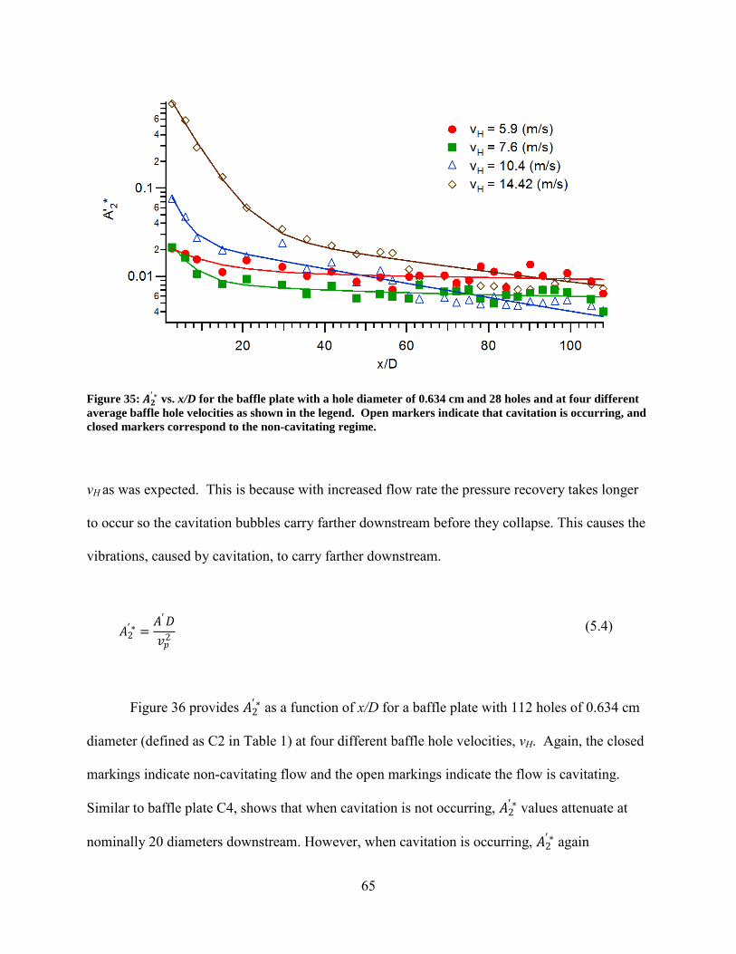
65
Figure 35: 𝑨𝑨𝟐𝟐′∗ vs. x/D for the baffle plate with a hole diameter of 0.634 cm and 28 holes and at four different average baffle hole velocities as shown in the legend. Open markers indicate that cavitation is occurring, and closed markers correspond to the non-cavitating regime.
vH as was expected. This is because with increased flow rate the pressure recovery takes longer
to occur so the cavitation bubbles carry farther downstream before they collapse. This causes the
vibrations, caused by cavitation, to carry farther downstream.
𝐴𝐴2′∗ =
𝐴𝐴′𝐷𝐷𝑣𝑣𝑝𝑝2
(5.4)
Figure 36 provides 𝐴𝐴2′∗ as a function of x/D for a baffle plate with 112 holes of 0.634 cm
diameter (defined as C2 in Table 1) at four different baffle hole velocities, vH. Again, the closed
markings indicate non-cavitating flow and the open markings indicate the flow is cavitating.
Similar to baffle plate C4, shows that when cavitation is not occurring, 𝐴𝐴2′∗ values attenuate at
nominally 20 diameters downstream. However, when cavitation is occurring, 𝐴𝐴2′∗ again

66
attenuates at increasing x/D locations with increasing vH. Data of this nature was obtained for all
baffle plates and the data of Figure 35 and Figure 36 is representative of the generally observed
behavior.
Figure 36: 𝑨𝑨𝟐𝟐′∗ vs. x/D for the baffle plate with a hole diameter of 0.634 cm and 112 holes and at four different average baffle hole velocities as shown in the legend. Open markers indicate that cavitation is occurring, and closed markers correspond to the non-cavitating regime.
Figure 37 is a plot of 𝐴𝐴2′∗ versus x/D for five baffle plates (being A1, B1, C2, D2, and E1
of Table 1) at a nominal baffle hole velocity of vH = 10.7 m/s all with a through area ratio of
AH/Ap = 43.8%. The closed markings indicate the flow is not cavitating and the open markings
indicate cavitation is present. This figure reveals that as the baffle hole diameter increases, the
attenuation of vibrations occur at increased normalized distance, x/D. This is likely due to the
fact that for decreased baffle hole diameter the number of holes increases, which in turn allows
for more interacting of the jets. As was discussed in section 2.1, if the number of interacting jets
increases the amount of turbulence from the jets is suppressed. The cavitation bubbles that form

67
within the turbulent eddies is forced to collapse at lower x/D locations because the eddies (that
are carrying the cavitation bubbles) rotational velocity is suppressed and the eddies die out.
Figure 37: 𝑨𝑨𝟐𝟐′∗ vs. x/D for five baffle plates with varying baffle hole diameter, d, with constant through area ratio (AH/Ap=0.438) and constant baffle hole velocity(vH = 10.7 m/s). Open markers indicate that cavitation is occurring, and closed markers correspond to the non-cavitating regime.
When cavitation is not present the data of Figure 37 again shows that the attenuation distance
occurs between 20 and 30 diameters, with the location increasing with increased baffle hole
diameter. Between an x/D location of 56 and 60 was where the two pipes were joined with a
flange.
The results discussed above show that the attenuation distance of pipe wall vibrations to
the no baffle plate level increases dramatically with the appearance of cavitation. It is also
discussed that the attenuation distance is highly dependent upon the baffle hole velocity, vH, and
the baffle hole diameter.

68
5.4 Summary of Observations from the Results
The following points summarize the important observations made in this chapter:
• The baffle plate loss coefficient was determined to be a function of both the
through area ratio and thickness to diameter ratio, with the loss increasing as
AH/Ap decreases.
• Cavitation inception occurs at higher fluid velocities for increasing thickness to
diameter ratio and increasing through area ratio. This point is very dependent
upon the magnitude of the loss coefficient.
• Vibration levels increase with decreased thickness to diameter ratio, and
decreased through area ratio for both the cavitating and non-cavitating regime,
and are also related to the loss coefficient.
• The attenuation distance of vibration levels when the flow is non-cavitating
occurs at nominally 20-30 diameters regardless of the flow velocity.
• The attenuation distance of vibration levels downstream of the baffle plate
increases dramatically when cavitation is present.
• The attenuation distance of vibration levels also increases with increased baffle
hole diameter and baffle hole velocity.

69
6 DEVELOPED MODELS
This chapter presents and gives a detailed discussion about the models that where
produced from the empirical data. A total of ten models have been produced from this work.
The use of these models will allow a designer to design for the pressure gradient loading caused
by turbulence and cavitation induced pipe vibrations. The purpose of the models is to 1) Predict
the cavitation design limits, 2) Predict the magnitude of A′ in the non-cavitation regime and up to
the critical cavitation design limit, and 3) Predict the streamwise distance from the baffle plate
when the vibration levels attenuate. Figure 38 is a representative plot of A′ vs. the cavitation
number, σ, which will be referred to throughout this chapter to describe the models that were
developed. Appendix A gives a description of how to use the models described in this section to
predict the critical values in a design application.
This chapter will first discuss the loss coefficient model produced in section 6.1. It will
then discuss the models produced for predicting the incipient and critical cavitation points in
section 6.2. The model for predicting the A′ levels at the incipient and critical cavitation points
will then be discussed in section 6.3. Following this a discussion on the models produced to
predict the pipe velocity at critical and incipient cavitation points in section 6.4. Section 6.5 will
discuss the model developed for predicting the slope of the non-cavitating regime (the black line
in Figure 38). Finally a discussion on the model developed for the attenuation data will be
presented in section 6.6.

70
Figure 38: A representative plot of A′ vs. the cavitation number, σ. The intersection of the red and black lines is the incipient cavitation design limit, σi, and the intersection of the blue and red lines is the critical cavitation design limit, σc.
6.1 Loss Coefficient
The loss coefficient is a very important parameter, due to the fact that cavitation
inception and vibration levels are a function of it as was revealed in chapter 5. Equation (6.1) is
a piecewise model that was produced to predict the loss coefficient based on all of the data at the
point of cavitation inception. It should be noted that the loss coefficient only varied by about 5%
before inception occurred. Thus, the model is useful in predicting KL during the entire range of
operation prior to cavitation. 𝜙𝜙 is defined in equation (6.2) and is a parameter that includes both
AH/Ap and t/d influences. This variable was developed from a multi-variable regression analysis.
The theoretical loss coefficient model, KLA, was discussed earlier and is defined in equation (6.3).
The α value is defined in equation (6.4) where Aj is the jet velocity from the vena-contracta. This

71
value is assumed in the models here to remain at a constant value of 0.72. This is because this
value created the best fit to the lower limit of the loss coefficient data as discussed in section 5.1.
This model was developed by a statistical analysis of the data and by modifying the KLA model
with the empirical results that were obtained to account for the variation of the loss coefficient as
a function of both the thickness to diameter ratio, t/d, and the through area ratio, AH/Ap.
𝐾𝐾𝐿𝐿𝐻𝐻 = �(2.9 − 3.79𝜙𝜙 + 1.79𝜙𝜙2)𝐾𝐾𝐿𝐿𝐴𝐴 , 𝜙𝜙 < 0.9
(0.876 + 0.069𝜙𝜙)𝐾𝐾𝐿𝐿𝐴𝐴 , 𝜙𝜙 ≥ 0.9�
(6.1)
𝜙𝜙 = �𝑡𝑡𝑑𝑑� �𝐴𝐴𝐻𝐻𝐴𝐴𝑝𝑝�
1/5
(6.2)
𝐾𝐾𝐿𝐿𝐴𝐴 = �1 − 2 �𝐴𝐴𝑝𝑝𝐴𝐴𝐻𝐻� + 2 �
𝐴𝐴𝑝𝑝𝐴𝐴𝐻𝐻�
2
�1 −1𝛼𝛼
+1
2𝛼𝛼2���𝐴𝐴𝐻𝐻𝐴𝐴𝑝𝑝�
2
(6.3)
𝛼𝛼 =𝐴𝐴𝑗𝑗𝐴𝐴𝐻𝐻
= 0.72 (6.4)
Figure 39 provides a plot of KLH/KLA versus 𝜙𝜙 for all 14 plates where cavitation was
observed (the AH/Ap = 0.609 baffle plate did not cavitate at the speeds explored). Data acquired
by Testud et. al. [13] are also shown in the figure for comparison. These two data points are for
both a single hole orifice (𝜙𝜙 =0.48) plate and a multi-hole orifice plate (𝜙𝜙 = 2.56). As illustrated
the data of Testud show excellent agreement with the present data and proposed model. The
model is divided by two functions that represent thin baffle plates (𝜙𝜙 ≤ 0.9) and a thick baffle
plate (𝜙𝜙 ≥ 0.9). Again, the thin baffle plate is for the plates where the flow does not reattach
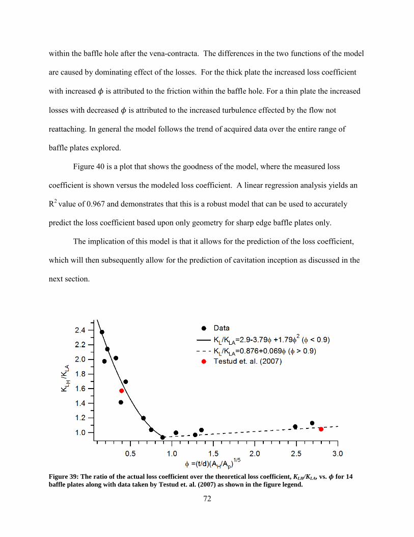
72
within the baffle hole after the vena-contracta. The differences in the two functions of the model
are caused by dominating effect of the losses. For the thick plate the increased loss coefficient
with increased 𝜙𝜙 is attributed to the friction within the baffle hole. For a thin plate the increased
losses with decreased 𝜙𝜙 is attributed to the increased turbulence effected by the flow not
reattaching. In general the model follows the trend of acquired data over the entire range of
baffle plates explored.
Figure 40 is a plot that shows the goodness of the model, where the measured loss
coefficient is shown versus the modeled loss coefficient. A linear regression analysis yields an
R2
value of 0.967 and demonstrates that this is a robust model that can be used to accurately
predict the loss coefficient based upon only geometry for sharp edge baffle plates only.
The implication of this model is that it allows for the prediction of the loss coefficient,
which will then subsequently allow for the prediction of cavitation inception as discussed in the
next section.
Figure 39: The ratio of the actual loss coefficient over the theoretical loss coefficient, KLH/KLA, vs. 𝝓𝝓 for 14 baffle plates along with data taken by Testud et. al. (2007) as shown in the figure legend.

73
Figure 40: The actual loss coefficient, KLH, vs. the modeled KLH of Eq. (6.1). The goodness of fit is shown with an R2
6.2 Incipient and Critical Cavitation Numbers
value of 0.967.
The incipient and critical cavitation numbers, σi and σc, are design limits of cavitation as
illustrated in Figure 38. As discussed in section 2.4.2 a study by Tullis [15] showed that the
cavitation number for orifices are dependent upon the size scaling effects as shown in equations
(6.5) and (6.6). The model for size scale effect, SSE, developed by Tullis [15] is shown in
equations (6.7) and (6.8). A model was developed based on the baffle plates of this study for the
incipient and critical cavitation numbers with the size scale effects (𝜎𝜎𝑖𝑖∗ and 𝜎𝜎𝑐𝑐∗) as a function of
the discharge coefficient. The models are given in equations (6.9) and (6.10). The discharge
coefficient, cd, (defined in equation (6.11)) is a function of the loss coefficient based off of the
pipe velocity, KLp as defined in equation (6.12). This model shows that the variation in cavitation

74
inception is primarily due to the loss coefficient and the size scale effects. This model was
developed by a linear regression analysis of the data where a curve was fit to the data.
𝜎𝜎𝑖𝑖 =𝜎𝜎𝑖𝑖∗
𝑆𝑆𝑆𝑆𝑆𝑆
(6.5)
𝜎𝜎𝑐𝑐 =𝜎𝜎𝑐𝑐∗
𝑆𝑆𝑆𝑆𝑆𝑆
(6.6)
𝑆𝑆𝑆𝑆𝑆𝑆 = �𝐷𝐷𝑑𝑑�𝑌𝑌
(6.7)
𝑌𝑌 = 0.3𝐾𝐾𝐿𝐿𝑝𝑝−0.25 (6.8)
𝜎𝜎𝑖𝑖∗ = −944𝑐𝑐𝑑𝑑4 + 1375𝑐𝑐𝑑𝑑3 − 663𝑐𝑐𝑑𝑑2 + 136𝑐𝑐𝑑𝑑 − 5.7 (6.9)
𝜎𝜎𝑐𝑐∗ = −685𝑐𝑐𝑑𝑑4 + 1026𝑐𝑐𝑑𝑑3 − 499𝑐𝑐𝑑𝑑2 + 102𝑐𝑐𝑑𝑑 − 4.3 (6.10)
𝑐𝑐𝑑𝑑 = 1
�𝐾𝐾𝐿𝐿𝑝𝑝+1 (6.11)
𝐾𝐾𝐿𝐿𝑝𝑝 = 𝐾𝐾𝐿𝐿𝐻𝐻 �𝐴𝐴𝐻𝐻𝐴𝐴𝑝𝑝�−2
(6.12)

75
Figure 41 and Figure 43 show plots of the incipient and critical cavitation numbers with
the sizes scale effects (𝜎𝜎𝑖𝑖∗ and 𝜎𝜎𝑐𝑐∗) versus the discharge coefficient, cd, for the 13 baffle plates the
models were developed from. The 2.54 cm diameter hole with 4 baffle holes (labeled as A2 in
Table 1) was not used in the models due to hole spacing being larger than the pipe section
causing added effects to cavitation inception that were not explored in this work. Also shown in
the figure is data for one baffle plate that was used by Testud et. al. [13]. As illustrated the data
of Testud et. al. show excellent agreement with the present data and proposed model. The data
point with the open marker is a baffle plate that had slight rounding of the holes due caused by
the manufacturing of the plate, and is included to illustrate the effect of rounding the baffle holes
and will be discussed further below. This data point illustrates that the models developed are for
sharp edged baffle plates only. From this figure it can be seen that there are two general trends
to the data. Above a discharge coefficient cd ≈ 4.0 both 𝜎𝜎𝑖𝑖∗ and 𝜎𝜎𝑐𝑐∗ increase linearly with cd. This
region corresponds to baffle plates that are relatively thick as was discussed in section 5.1 in
regards to the loss coefficient, with a discharge coefficient below cd ≈ 4.0 both 𝜎𝜎𝑖𝑖∗ and 𝜎𝜎𝑐𝑐∗
increase exponentially to an asymptotic value of 𝜎𝜎𝑖𝑖∗ = 5 and 𝜎𝜎𝑐𝑐∗ = 4 respectively. In general the
model follows the trend of acquired data over the entire range of baffle plates explored.
Figure 42 and Figure 44 are plots that show the goodness of the model, where the
measured 𝜎𝜎𝑖𝑖∗ and 𝜎𝜎𝑐𝑐∗ is shown versus the modeled 𝜎𝜎𝑖𝑖∗ and 𝜎𝜎𝑐𝑐∗. A linear regression analysis yields
an R2 value of 0.997 and 0.978, respectively. This demonstrates that two models for 𝜎𝜎𝑖𝑖∗ and 𝜎𝜎𝑐𝑐∗
are robust models that can be used to accurately predict σi and σc based off of the geometry and
the loss coefficient, that can be predicted from the model in the previous section.
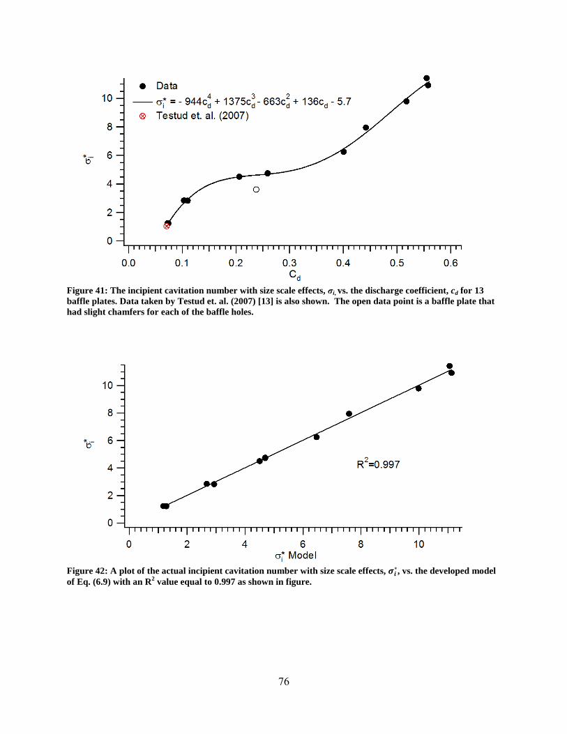
76
Figure 41: The incipient cavitation number with size scale effects, σi, vs. the discharge coefficient, cd for 13 baffle plates. Data taken by Testud et. al. (2007) [13] is also shown. The open data point is a baffle plate that had slight chamfers for each of the baffle holes.
Figure 42: A plot of the actual incipient cavitation number with size scale effects, 𝝈𝝈𝒊𝒊∗, vs. the developed model of Eq. (6.9) with an R2 value equal to 0.997 as shown in figure.
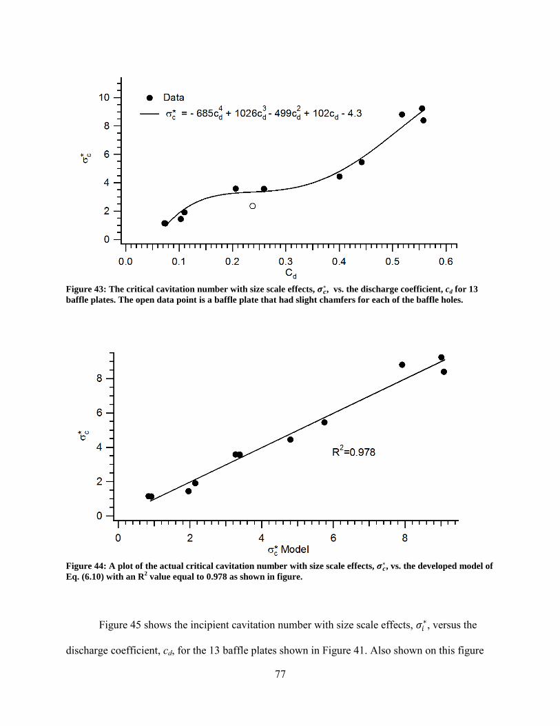
77
Figure 43: The critical cavitation number with size scale effects, 𝝈𝝈𝒄𝒄∗, vs. the discharge coefficient, cd for 13 baffle plates. The open data point is a baffle plate that had slight chamfers for each of the baffle holes.
Figure 44: A plot of the actual critical cavitation number with size scale effects, 𝝈𝝈𝒄𝒄∗, vs. the developed model of Eq. (6.10) with an R2
Figure 45
value equal to 0.978 as shown in figure.
shows the incipient cavitation number with size scale effects, 𝜎𝜎𝑖𝑖∗, versus the
discharge coefficient, cd, for the 13 baffle plates shown in Figure 41. Also shown on this figure

78
are data acquired by Testud et. al. (2007) [13], data from Tullis et. al. (1980) [9] for multi-hole
orifice plates with rounding of the baffle holes at a radius of 0.9525 cm for the inlet of each hole,
and data from Tullis (1989) [15] for a sharp edged single hole orifice. The open circle data point
is again the outlier caused by a baffle plate that had slight chamfer for each of the baffle holes.
This plot reveals the influence of rounding, and multiple holes. It can be seen that a multi-hole
orifice plate has larger 𝜎𝜎𝑖𝑖∗ overall as compared to the single hole orifice. With increased
rounding of a hole the baffle plate approaches the single hole orifice plate solution. The model
that was developed as described above does not account for the effects of rounding the baffle
holes. Further work will be needed to account for the effect of round the baffle holes.
Figure 45: The incipient cavitation number with size scale effects, 𝝈𝝈𝒊𝒊∗, vs. the discharge coefficient, cd for 13 baffle plates. Data taken by Testud et. al. (2007) [13], data from Tullis et. al. (1980) [9] for multi-hole orifice plates with rounding of 0.9525 cm for the inlet of each hole, and data from Tullis (1989) [15] for a single hole orifice is also shown. The open circle data point is an outlier caused by a baffle plate that had slight chamfers for each of the baffle holes.

79
The models that were developed above for the incipient and critical cavitation points
allow a designer to determine when cavitation will occur and when the flow has reached full
cavitation. Conversely, the designer can utilize the models to determine the correct geometry of
a baffle plate that will allow for the flow to stay below the undesirable cavitating range at
specific flow rates.
6.3 A′ at Critical and Incipient Cavitation
The RMS of the pipe wall acceleration, A′, is used to characterize the vibrations of the
pipe. The models developed for A′ levels at incipient and critical cavitation points allow a
designer to understand the loading that a pipe will experience at these design limits. The A′
value at incipient and critical cavitation levels are illustrated in Figure 38. Equations (6.13) and
(6.14) provide the models developed for the non-dimensionalized A′ levels at the point of
incipient and the point of critical cavitation. The non-dimensionalized A′ values (𝐴𝐴𝑖𝑖′∗ and 𝐴𝐴𝑐𝑐′∗) are
defined in equations (6.15) and (6.16) and the βi and βc values are defined in equations (6.17) and
(6.18). These models were developed by performing a multi-variable linear regression analysis
of the data, were βi and βc were produced from this analysis.
𝑙𝑙𝑛𝑛(𝐴𝐴𝑖𝑖′∗) = 0.038 (𝑙𝑙𝑛𝑛(𝛽𝛽𝑖𝑖))3 − 0.45 (𝑙𝑙𝑛𝑛(𝛽𝛽𝑖𝑖))2 + 0.039 𝑙𝑙𝑛𝑛(𝛽𝛽𝑖𝑖) − 8.86) (6.13)
𝑙𝑙𝑛𝑛(𝐴𝐴𝑐𝑐′∗) = 0.028 (𝑙𝑙𝑛𝑛(𝛽𝛽𝑐𝑐))3 − 0.33(𝑙𝑙𝑛𝑛(𝛽𝛽𝑐𝑐))2 − 0.35 𝑙𝑙𝑛𝑛(𝛽𝛽𝑐𝑐)− 6.74 (6.14)

80
𝐴𝐴𝑖𝑖′∗ =𝐴𝐴𝑖𝑖′ 𝑑𝑑𝑣𝑣𝐻𝐻𝑖𝑖
2 (6.15)
𝐴𝐴𝑐𝑐′∗ =𝐴𝐴𝑐𝑐′ 𝑑𝑑𝑣𝑣𝐻𝐻𝑐𝑐
2 (6.16)
𝛽𝛽𝑖𝑖 = 𝜎𝜎𝑖𝑖 �𝑡𝑡𝑑𝑑�
1.8�𝐴𝐴𝐻𝐻𝐴𝐴𝑝𝑝�−0.6
(6.17)
𝛽𝛽𝑐𝑐 = 𝜎𝜎𝑐𝑐 �𝑡𝑡𝑑𝑑�
1.8�𝐴𝐴𝐻𝐻𝐴𝐴𝑝𝑝�−0.6
(6.18)
Figure 46 and Figure 48 are plots of the natural logarithm of the non-dimensionalized A′
value at the incipient and critical cavitation points (𝐴𝐴𝑖𝑖′∗ and 𝐴𝐴𝑐𝑐′∗) versus the natural logarithm of βi
and βc for the baffle plates used. For the 𝐴𝐴𝑐𝑐′∗ model only 12 plates were used since the range of
velocities for plate D1 of Table 1 was not high enough to obtain the critical cavitation value.
This figure shows that there is a local maximum of vibrations around ln(β) = 0. In general these
models follow the trend of acquired data over the entire range of baffle plates explored.
Figure 47 and Figure 49 are plots that show the goodness of the model, where the
measured 𝐴𝐴𝑖𝑖′∗ and 𝐴𝐴𝑐𝑐′∗ is shown versus the modeled 𝐴𝐴𝑖𝑖′∗ and 𝐴𝐴𝑐𝑐′∗. A linear regression analysis
yields a R2
value of 0.964 and 0.984, respectively. This demonstrates that two models for 𝐴𝐴𝑖𝑖′∗
and 𝐴𝐴𝑐𝑐′∗ are robust models that can be used to accurately predict 𝐴𝐴𝑖𝑖′∗ and 𝐴𝐴𝑐𝑐′∗ based off of the
geometry and the σi and σc values, that can be determined from the models in the previous
section.

81
Figure 46: ln(𝑨𝑨𝒊𝒊′∗) as a function of βi for 13 baffle plate.
Figure 47: A plot of the actual 𝑨𝑨𝒊𝒊′∗vs. the model developed in Eq. (6.13) with an R2 value equal to 0.964 as shown in figure.
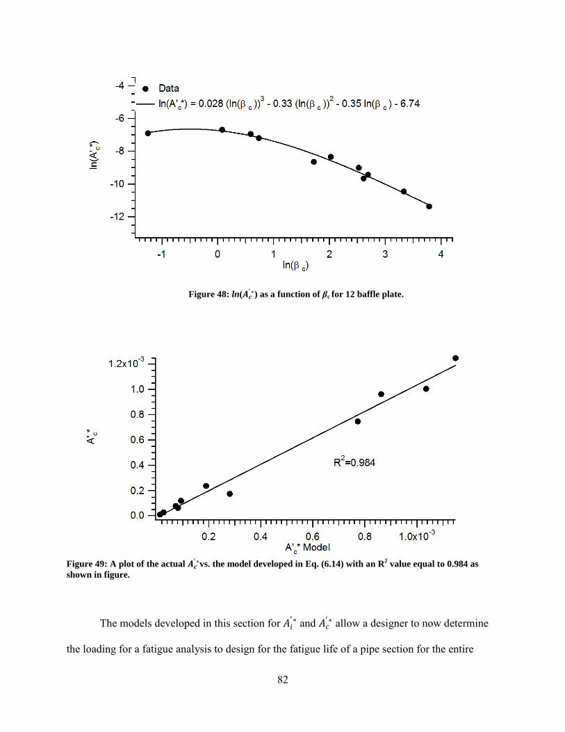
82
Figure 48: ln(𝑨𝑨𝒄𝒄′∗) as a function of βc for 12 baffle plate.
Figure 49: A plot of the actual 𝑨𝑨𝒄𝒄′∗vs. the model developed in Eq. (6.14) with an R2
The models developed in this section for 𝐴𝐴𝑖𝑖′∗ and 𝐴𝐴𝑐𝑐′∗ allow a designer to now determine
the loading for a fatigue analysis to design for the fatigue life of a pipe section for the entire
value equal to 0.984 as shown in figure.

83
incipient cavitation regime (the red line in Figure 38). This is because the points (σi, 𝐴𝐴𝑖𝑖′∗) and (σc,
𝐴𝐴𝑐𝑐′∗) from Figure 38 can be solved for and the A′ versus σ curve between these two points is
linear on a log-log scale. This allows for prediction of the cavitation induced vibration between
these two important points.
6.4 The Incipient and Critical Velocities
The incipient and critical velocities (vpi and vpc) are the average pipe velocities at the
point of cavitation inception and critical cavitation. The purpose for obtaining the model of the
vpi and vpc is so that the A′ can be determined. The models that were developed in section 6.3
were for 𝐴𝐴𝑖𝑖′∗ and 𝐴𝐴𝑐𝑐′∗, the non-dimensionalized A′ levels that were normalized by the baffle hole
velocities. The models that were developed for vpi and vpc are given in equations (6.19) and
(6.20). The value ψ is defined in equation (6.21) which is a parameter that includes both cd and
t/d influences. This variable was produced from the multi-variable linear regression analysis that
was performed to create the models. As can be seen both vpi and vpc are linear functions of ψ.
𝑣𝑣𝑝𝑝𝑖𝑖 = 8.65 𝜓𝜓 + 0.11 (6.19)
𝑣𝑣𝑝𝑝𝑐𝑐 = 10.64 𝜓𝜓 + 0.1 (6.20)
𝜓𝜓 = 𝑐𝑐𝑑𝑑 �𝑡𝑡𝑑𝑑�
0.15
(6.21)
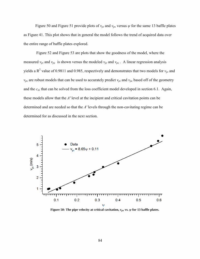
84
Figure 50 and Figure 51 provide plots of vpi and vpc versus ψ for the same 13 baffle plates
as Figure 41. This plot shows that in general the model follows the trend of acquired data over
the entire range of baffle plates explored.
Figure 52 and Figure 53 are plots that show the goodness of the model, where the
measured vpi and vpc is shown versus the modeled vpi and vpc . A linear regression analysis
yields a R2
6.1
value of 0.9811 and 0.985, respectively and demonstrates that two models for vpi and
vpc are robust models that can be used to accurately predict vpi and vpc based off of the geometry
and the cd, that can be solved from the loss coefficient model developed in section . Again,
these models allow that the A′ level at the incipient and critical cavitation points can be
determined and are needed so that the A′ levels through the non-cavitating regime can be
determined for as discussed in the next section.
Figure 50: The pipe velocity at critical cavitation, vpi, vs. ψ for 13 baffle plates.

85
Figure 51: The pipe velocity at critical cavitation, vpc, vs. ψ for 13 baffle plates.
Figure 52: A plot of the actual vpi vs. the model developed in Eq. (6.19) showing an R2 value equal to 0.981 as shown in figure.

86
Figure 53: A plot of the actual vpc vs. the model developed in Eq. (6.20) showing an R2
6.5 Slope for Non-Cavitating Regime
value equal to 0.985 as shown in figure.
The flow induced vibrations of a pipe is not limited to cavitation alone. When the flow is
not cavitating vibrations of a pipe wall occur from turbulence, as was discussed in section 6.2.
For a designer, a model of the turbulent induced vibrations from a baffle plate is needed for
analysis when cavitation is not occurring in a flow. To develop models of the turbulent induced
vibrations a model of the slope of the non-cavitating regime, m, (this is the slope of the black line
in Figure 38) is developed. By knowing this slope, the A′ levels through the non-cavitating
regime can be determined. This is due to the fact that the point ( σi, A′) is known by using the
models of the previous sections. This allows for the development of a non-cavitating turbulent
induced model. The model that was developed is shown in equation (6.22) where m* is defined

87
in equation (6.23) and ε is defined in equation (6.24). Both m* and ε are produced from the
multi-variable linear regression analysis that was used to create the model.
𝑚𝑚∗ = 1.2 − 0.72 𝑒𝑒𝑥𝑥𝑝𝑝(−252𝜀𝜀)− 0.38 𝑒𝑒𝑥𝑥𝑝𝑝(−1840𝜀𝜀) (6.22)
𝑚𝑚∗ =𝑚𝑚
2 𝑙𝑙𝑛𝑛 �𝐴𝐴𝐻𝐻𝐴𝐴𝑝𝑝� − 0.4
(6.23)
𝜀𝜀 = �𝑑𝑑𝐷𝐷� �𝑡𝑡𝑑𝑑�
0.4�𝐴𝐴𝐻𝐻𝐴𝐴𝑝𝑝�
2.5
(6.24)
Figure 54 is a plot of m* versus ε for the same 13 baffle plates of Figure 50 where
cavitation was observed. In general the model follows the trend of acquired data over the entire
range of baffle plates explored.
Figure 55 show the goodness of the model, where the measured m* is shown versus the
modeled m*. A linear regression analysis yields an R2
Figure 38
value of 0.976, and demonstrates that the
model for m* is a robust models that can be used to accurately predict the slope of the black line
in based off of the geometry of the baffle plate. Again, this model allows for prediction
of vibration levels throughout the entire turbulent regime.
The models developed in the above sections can now be used to predict a figure similar to
Figure 38 for any sharp edged baffle plate geometry. A discussion on how to do so is discussed
in Appendix A. Creating a plot of this nature provides the desired A′ levels to be known for all
flow rates up to the critical design limit for any sharp edged baffle plate geometry.

88
Figure 54: A plot of m* as a function of ε for 13 baffle plates
Figure 55: A plot of the actual m* value vs. the model developed in Eq. (6.22) showing an R2 value equal to 0.976 as shown in figure.

89
6.6 Attenuation of Vibration
The models developed in the previous sections are used to predict the vibration levels that
occur at three diameters downstream from the baffle plate. Because the vibration levels caused
from the flow through the baffle plate attenuated downstream as discussed in section 5.3, a
model for this attenuation also was developed. Equation (6.26) shows the model that was
developed for the attenuation distance. The model is a function of both the baffle hole velocity,
vH, and the baffle hole velocity at the point of cavitation inception, vHi. vHi can be obtained by
knowing vpi from the model discussed in section 6.4 and by using the continuity equation shown
in equation (6.25).
𝑣𝑣𝐻𝐻𝑖𝑖 = 𝑣𝑣𝑝𝑝𝑖𝑖 �𝐴𝐴𝑝𝑝𝐴𝐴𝐻𝐻
� (6.25)
𝑥𝑥𝐷𝐷≅ �
20 𝑡𝑡𝑡𝑡 30, 𝑣𝑣𝐻𝐻/𝑣𝑣𝐻𝐻𝑖𝑖 < 1
120𝑣𝑣𝐻𝐻𝑣𝑣𝐻𝐻𝑖𝑖
− 75, 1 ≤𝑣𝑣𝐻𝐻𝑣𝑣𝐻𝐻𝑖𝑖
≥ 1.5
105 𝑡𝑡𝑡𝑡 110, 𝑣𝑣𝐻𝐻/𝑣𝑣𝐻𝐻𝑖𝑖 > 1.5
�
(6.26)
Figure 56 shows the x/D location where the vibration levels attenuate downstream of the
baffle plate as a function of the ratio of the baffle hole velocity over the baffle hole velocity at
cavitation inception, v/vHi, for a given plate. In the figure the attenuation distance was defined to
be the x/D location where 𝐴𝐴2′∗ had decayed to 1.5 times the 𝐴𝐴2
′∗ level of the non-baffle plate
condition at the same pipe velocity. 𝐴𝐴2′∗ is again defined in equation (6.27). This figure shows
that with exception of a few outliers the general trend of the attenuation of vibrations

90
downstream of a baffle plate. When cavitation is not occurring vH/vHi ≤ 1.0 the attenuation of
vibrations occurs no greater than 20 to 30 x/D locations. When cavitation is occurring vH/vHi ≥
1.0 and vH/vHi ≤ 1.5 the x/D location of the attenuation of vibrations increase dramatically with
increased vH/vHi where vH/vHi ≥ 1.5 the x/D location of the attenuation of vibrations occurs no
greater than 105 to 110. This model allows for an estimate for how the A′ attenuated
downstream.
𝐴𝐴2′∗ =
𝐴𝐴′𝐷𝐷𝑣𝑣𝑝𝑝2
(6.27)
Figure 56: The attenuation of vibration levels downstream of the baffle plate, x/D, vs. Re/Rei.

91
7 CONCLUSIONS
7.1 Summary of Results
A study on the cavitation and turbulent induced pipe vibrations caused by 16 sharp edge
baffle plates was conducted. Cavitation and turbulent induced pipe vibrations were characterized
as a function of the geometry of the baffle plates. The following key findings of this work are
listed below:
• The baffle plate loss coefficient was determined to be a function of both the
through area ratio and thickness to diameter ratio, and the number of baffle holes.
• Cavitation inception occurs at higher fluid velocities with increased thickness to
diameter ratio where the baffle hole velocity varies from nominally 7 m/s to 13
m/s from a t/d ratio of 0.25 to 3.3 for AH/Ap = 43.8%.
• Cavitation inception occurs at higher fluid velocities with increased through area
ratio where the baffle hole velocity varies from nominally 9.5 m/s to 13 m/s from
a AH/Ap ratio of 10.9% to 43.8% for t/d = 1.7.
• Cavitation inception is a function of the radius of curvature of the baffle holes and
rounding can delay cavitation inception.
• Vibration levels increase with decreased plate thickness to hole diameter ratio by
about an order of magnitude for a range of t/d of 0.25 to 3.3,
• Vibration levels doubled with a decrease in AH/Ap ratio from 43.8% to 10.9%.

92
• The attenuation of vibration levels when the flow is non-cavitating occurs at
increasing flow rates up until nominally 20-30 diameters regardless of the flow
velocity.
• The attenuation of vibration levels within the cavitating regime dramatically
increases with increased flow rate from nominally 20 to 100 diameters. At
average baffle fluid velocities above 1.5 times the incipient baffle fluid velocity,
the attenuation distance is nominally 100-110 diameters
• Models predicting the loss coefficient, incipient and critical cavitation numbers,
and the RMS of the pipe wall acceleration, A′, from non-cavitating flow to the
critical cavitation level, have been developed
7.2 Recommendations
The recommendations for future work are as follows:
• Testing of actual valves and trims to evaluate how they perform relative to the
developed models.
• Explore the effects of rounding the baffle hole.
• Further validation of models with baffle plates for larger discharge coefficients
that were not explored.
• Further validation of models with varying pipe diameters.

93
REFERENCES
[1] S.H. Bush, "Failure Mechanisms in Nuclear Power Plants Piping Systems," Journal of pressure vessel technology, vol. 114, no. 4, pp. 389-395, November 1992.
[2] Mao Qing, Zhang Jinghui, Luo Yushan, Wang Haijun, and Duan Quan, "High-Level Vibration and Noise Analysis of Nuclear Pipes with Orifice," in Transactions of the 17th Internation Confrence on Structural Mechanics in Reactor Technology, Prague, Czech Republic, August 17-22, 2003, pp. O02-6.
[3] National Transportation Safety Board, "Pipeline Accident Brief," NTSB/PAR-04/01, Pipeline accident number: PB2004-916501, July 4, 2002.
[4] David C. Wilcox, Turbulence Modeling for CFD 3rd.: DCW Industries, Inc., 2006.
[5] Matthew T. Pittard, Robert P. Evans, R. Daniel Maynes, and Jonathan D. Blotter, "Experimental and Numerical Investigation of Turbulent Flow Induced Pipe Vibration in Fully Developed Flow," Review of Scientific Instruments, vol. 75, pp. 2393-2401, July 2004.
[6] Robert P. Evans, Jonathan D. Blotter, and Alan G. Stephens, "Flow Rate Measurements Using Flow-Induced Pipe Vibration," Transactions of the ASME, vol. 126, pp. 280-285, March 2004.
[7] Andrew Thompson, "Experimental Charactarization of Flow Induced Vibration in Turbulent Pipe Flow," Brigham Young University, Provo, Master's Thesis 2009.
[8] Andrew S. Thompson, Daniel Maynes, Thomas Shurtz, and Jonathan D. Blotter, "Experimental Characterization of Flow Induced Vibration in Fully Developed Turbulent Pipe Flow," in Proceedings of the ASME Fluids Engineering Summer Meeting, August 2009, pp. 1771-1778.
[9] J. Paul Tullis, James J. Powers III, Paul F. Shiers, and Whitney W. Hall, "Perforated Plates as Hydraulic Energy Dissipators," in Computer and Physical Modeling in Hydraulic Engineering, August 1980, pp. 62-73.
[10] F. Numachi, M. Yamabe, and R. OBA, "Cavitation Effect on the Discharge Coefficient of the Sharp-Edged Orifice Plate," Journal of Basic Engineering, vol. 82, pp. 1-11, March 1960.
[11] P. A. Kolodzie and Matthew Van Winkle, "Discharge Coefficients Through Perforated Plates," AICHE Journal, vol. 3, pp. 305-312, September 1957.

94
[12] Bruce R. Munson, Donald F. Young, and Theodore H. Okiishi, Fundamentals of Fluid Mechanics 5th.: John Wiley & Sons, 2006.
[13] P. Testud, P. Moussou, A. Hirschburg, and Y. Auregan, "Noise Generated by Cavitating Single-hole and Multi-hole Orifices in a Water Pipe," Journal of Fluids and Structures, vol. 23, pp. 163-189, February 2007.
[14] J. Paul Tullis, M. ASCE, and Rangachari Govindarajan, "Cavitation and Size Scale Effects for Orifices," ASCE Journal of Hydraulics Division, vol. 97, pp. 417–430, March 1973.
[15] J. Paul Tullis, Hydraulics of Pipelines Pumps, Valves, Cavitation, Transients.: John Wiley & Sons, 1989.
[16] S. C. Li, Cavitation of Hydraulic Machinery.: Imperial College Press, 2000.
[17] Yves Lecoffre, Cavitation Bubble Trackers.: AA Balkema Publishers, 1999.
[18] J. Paul Tullis, "Cavitation Guide for Control Valves," US Nuclear Regulatory Commission, April 1993.
[19] Mao Qing, Zhang Jinghui, Luo Yushan, Wang Haijun, and Duan Quan, "Experimental Studies of Orifice-induced Wall Pressure Fluctuations and Pipe Vibration," Internation Journal of Pressure Vessels and Piping, vol. 83, pp. 505-511, March 2006.
[20] John Lawson and John Erjavec, Modern Statistics for Engineering and Quality Improvement. Pacific Grove, CA: Wadsworth Group, 2001.
[21] Richard S. Figliola and Donald E. Beasley, Theory and Design for Mechanical Measurements , 4th ed. Danvers, MA: John Wiley and Sons, Inc., 2006.

95
APPENDIX A. INSTRUCTIONS ON USE OF MODELS
To illustrate how to properly use the developed models the following example is provided.
Example:
If a baffle plate with a hole size of 0.634 cm with thickness of 0.67 cm and number of
holes of 112 was designed for a 10.16 cm pipe with a working fluid of water, what would be the
acceleration levels for a range of cavitation numbers up to the critical design limit?
Solution:
First the loss coefficient will be needed and can be found using equations (6.1)-(6.4).
𝜙𝜙 = �𝑡𝑡𝑑𝑑� �𝐴𝐴𝐻𝐻𝐴𝐴𝑝𝑝�
15
= 1.01 (A. 1)
𝐾𝐾𝐿𝐿𝐴𝐴 = �1 − 2 �𝐴𝐴𝑝𝑝𝐴𝐴𝐻𝐻� + 2 �
𝐴𝐴𝑝𝑝𝐴𝐴𝐻𝐻�
2
�1 −1𝛼𝛼
+1
2𝛼𝛼2���𝐴𝐴𝐻𝐻𝐴𝐴𝑝𝑝�
2
= 0.47 (A. 2)
𝐾𝐾𝐿𝐿𝐻𝐻 = (0.876 + 0.069𝜙𝜙)𝐾𝐾𝐿𝐿𝐴𝐴 = 0.44 (A. 3)

96
Now knowing the loss coefficient the discharge coefficient can be obtained so as to find
the values for the incipient and critical cavitation numbers. These values can be obtained using
equations (6.5)-(6.12).
𝐾𝐾𝐿𝐿𝑝𝑝 = 𝐾𝐾𝐿𝐿𝐻𝐻 �𝐴𝐴𝐻𝐻𝐴𝐴𝑝𝑝�−2
= 2.33 (A. 4)
𝑐𝑐𝑑𝑑 =1
�𝐾𝐾𝐿𝐿𝑝𝑝 + 1= 0.55 (A. 5)
𝜎𝜎𝑖𝑖∗ = −944𝑐𝑐𝑑𝑑4 + 1375𝑐𝑐𝑑𝑑3 − 663𝑐𝑐𝑑𝑑2 + 136𝑐𝑐𝑑𝑑 − 5.7 = 10.91 (A. 6)
𝜎𝜎𝑖𝑖 =𝜎𝜎𝑖𝑖∗
𝑆𝑆𝑆𝑆𝑆𝑆= 5.55
(A. 7)
𝜎𝜎𝑐𝑐∗ = −685𝑐𝑐𝑑𝑑4 + 1026𝑐𝑐𝑑𝑑3 − 499𝑐𝑐𝑑𝑑2 + 102𝑐𝑐𝑑𝑑 − 4.3 = 8.85 (A. 8)
𝜎𝜎𝑐𝑐 =𝜎𝜎𝑐𝑐∗
𝑆𝑆𝑆𝑆𝑆𝑆= 4.51
(A. 9)
With the incipient and critical cavitation numbers determined the 𝐴𝐴′∗ at the incipient and
critical cavitation values can be obtained using equations (6.13)-(6.18).
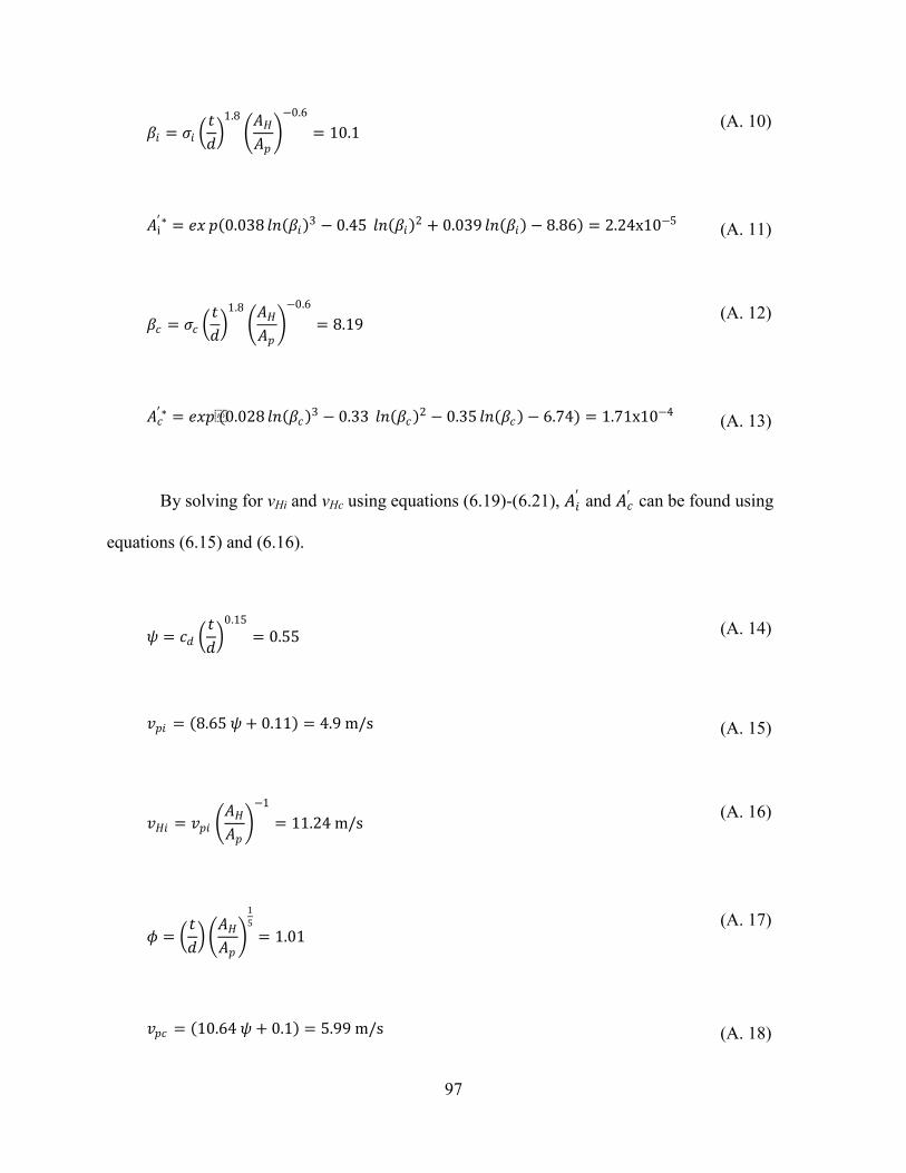
97
𝛽𝛽𝑖𝑖 = 𝜎𝜎𝑖𝑖 �𝑡𝑡𝑑𝑑�
1.8�𝐴𝐴𝐻𝐻𝐴𝐴𝑝𝑝�−0.6
= 10.1 (A. 10)
𝐴𝐴i′∗ = 𝑒𝑒𝑥𝑥 𝑝𝑝(0.038 𝑙𝑙𝑛𝑛(𝛽𝛽𝑖𝑖)3 − 0.45 𝑙𝑙𝑛𝑛(𝛽𝛽𝑖𝑖)2 + 0.039 𝑙𝑙𝑛𝑛(𝛽𝛽𝑖𝑖) − 8.86) = 2.24x10⁻⁵ (A. 11)
𝛽𝛽𝑐𝑐 = 𝜎𝜎𝑐𝑐 �𝑡𝑡𝑑𝑑�
1.8�𝐴𝐴𝐻𝐻𝐴𝐴𝑝𝑝�−0.6
= 8.19 (A. 12)
𝐴𝐴𝑐𝑐′∗ = 𝑒𝑒𝑥𝑥𝑝𝑝(0.028 𝑙𝑙𝑛𝑛(𝛽𝛽𝑐𝑐)3 − 0.33 𝑙𝑙𝑛𝑛(𝛽𝛽𝑐𝑐)2 − 0.35 𝑙𝑙𝑛𝑛(𝛽𝛽𝑐𝑐) − 6.74) = 1.71x10⁻⁴ (A. 13)
By solving for vHi and vHc using equations (6.19)-(6.21), 𝐴𝐴𝑖𝑖′ and 𝐴𝐴𝑐𝑐′ can be found using
equations (6.15) and (6.16).
𝜓𝜓 = 𝑐𝑐𝑑𝑑 �𝑡𝑡𝑑𝑑�
0.15= 0.55
(A. 14)
𝑣𝑣𝑝𝑝𝑖𝑖 = (8.65 𝜓𝜓 + 0.11) = 4.9 m/s (A. 15)
𝑣𝑣𝐻𝐻𝑖𝑖 = 𝑣𝑣𝑝𝑝𝑖𝑖 �𝐴𝐴𝐻𝐻𝐴𝐴𝑝𝑝�−1
= 11.24 m/s (A. 16)
𝜙𝜙 = �𝑡𝑡𝑑𝑑� �𝐴𝐴𝐻𝐻𝐴𝐴𝑝𝑝�
15
= 1.01 (A. 17)
𝑣𝑣𝑝𝑝𝑐𝑐 = (10.64 𝜓𝜓 + 0.1) = 5.99 m/s (A. 18)

98
𝑣𝑣𝐻𝐻𝑐𝑐 = 𝑣𝑣𝑝𝑝𝑐𝑐 �𝐴𝐴𝐻𝐻𝐴𝐴𝑝𝑝�−1
= 13.74 m/s (A. 19)
𝐴𝐴𝑖𝑖′ =𝐴𝐴𝑖𝑖′∗𝑣𝑣𝐻𝐻𝑖𝑖2
𝑑𝑑= 0.45
(A. 20)
𝐴𝐴𝑐𝑐′ =𝐴𝐴𝑐𝑐′∗𝑣𝑣𝐻𝐻𝑐𝑐2
𝑑𝑑= 5.09
(A. 21)
Figure 57 shows the design limits that have been solved for on a plot of A′ versus σ. By
knowing 𝐴𝐴𝑖𝑖′ , 𝐴𝐴𝑐𝑐′ , and the cavitation numbers at both the incipient and critical values, 𝐴𝐴′ is now
known for the entire incipient cavitation regime (The red line in Figure 57). This is because we
know that the 𝐴𝐴′ within the region between the incipient and critical cavitation values is linear
with σ on a log-log scale. An equation for this section can now be developed, where m2 is the
slope of the line and y2 is the y-intercept.
𝑙𝑙𝑛𝑛(𝐴𝐴′) = 𝑚𝑚2 𝑙𝑙𝑛𝑛(𝜎𝜎) + 𝑦𝑦2 (A. 22)
𝑚𝑚2 =𝑙𝑙𝑛𝑛(𝐴𝐴𝑐𝑐′ ) − 𝑙𝑙𝑛𝑛(𝐴𝐴𝑖𝑖′ )𝑙𝑙𝑛𝑛(𝜎𝜎𝑐𝑐) − 𝑙𝑙𝑛𝑛(𝜎𝜎i)
= −11.65 (A. 23)
𝑦𝑦2 = 𝑙𝑙𝑛𝑛(𝐴𝐴𝑖𝑖′ ) − 𝑐𝑐𝑙𝑙𝑡𝑡𝑝𝑝𝑒𝑒2 𝑙𝑙𝑛𝑛(𝜎𝜎𝑖𝑖) = 19.17 (A. 24)
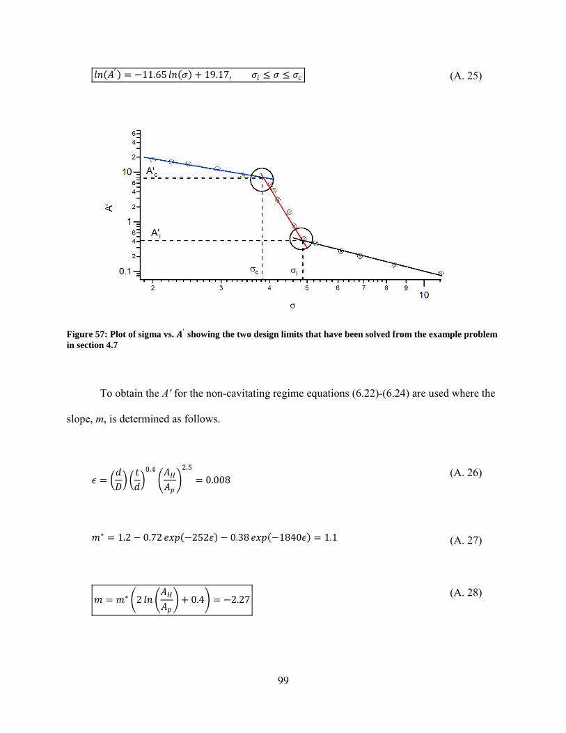
99
𝑙𝑙𝑛𝑛(𝐴𝐴′) = −11.65 𝑙𝑙𝑛𝑛(𝜎𝜎) + 19.17, 𝜎𝜎𝑖𝑖 ≤ 𝜎𝜎 ≤ 𝜎𝜎𝑐𝑐 (A. 25)
Figure 57: Plot of sigma vs. 𝑨𝑨′ showing the two design limits that have been solved from the example problem in section 4.7
To obtain the A′ for the non-cavitating regime equations (6.22)-(6.24) are used where the
slope, m, is determined as follows.
𝜖𝜖 = �𝑑𝑑𝐷𝐷� �𝑡𝑡𝑑𝑑�
0.4�𝐴𝐴𝐻𝐻𝐴𝐴𝑝𝑝�
2.5
= 0.008 (A. 26)
𝑚𝑚∗ = 1.2 − 0.72 𝑒𝑒𝑥𝑥𝑝𝑝(−252𝜀𝜀)− 0.38 𝑒𝑒𝑥𝑥𝑝𝑝(−1840𝜖𝜖) = 1.1 (A. 27)
𝑚𝑚 = 𝑚𝑚∗ �2 𝑙𝑙𝑛𝑛 �𝐴𝐴𝐻𝐻𝐴𝐴𝑝𝑝�+ 0.4� = −2.27
(A. 28)

100
An equation can now be developed for A′ as a function of σ for the non-cavitating regime
(black line in Figure 57) by using the slope, m, and the incipient point solved for above to find
the y-intercept, y.
𝑦𝑦 = − 𝑙𝑙𝑛𝑛(𝐴𝐴𝑖𝑖′ ) −𝑚𝑚 𝑙𝑙𝑛𝑛(𝜎𝜎𝑖𝑖) = 3.09 (A. 29)
ln(𝐴𝐴′) = −2.27 ln(𝜎𝜎) + 3.09, 𝜎𝜎 ≤ 𝜎𝜎𝑖𝑖 (A. 30)
A model of 𝐴𝐴𝐻𝐻′ up to the critical cavitation point has now been developed and can be seen
below. In Figure 58 a plot of A′ versus σ is shown comparing the actual measured data against
the model that was developed.
ln(𝐴𝐴′) = � −2.27 ln(𝜎𝜎) + 3.09, 𝜎𝜎 ≤ 𝜎𝜎𝑖𝑖−9.72 𝑙𝑙𝑛𝑛(𝜎𝜎) + 15.32, 𝜎𝜎𝑖𝑖 ≤ 𝜎𝜎 ≤ 𝜎𝜎𝑐𝑐
� (A. 31)
Figure 58: Plot of A′ vs. σ comparing experimental results to a model that was developed in equation (A.31) for a baffle plate with d=0.634 t=0.67 and n=112.

101
APPENDIX B. KEY PARAMETERS FOR ALL BAFFLE PLATES CONSIDERED
Table 4: Key parameters for all baffle plates considered
d (m)
t (m)
# holes (-)
KLp (-)
σi (-)
A′i (m/s2
vHi (m/s) )
σc (-)
A′c (m/s2
vHc (m/s) )
2.520 0.660 7 5.23 4.745 0.226 6.875 3.37 8.747 8.835 2.535 0.645 4 33.69 2.74 0.376 5.635 2.25 6.209 6.35 1.267 0.663 28 4.12 5.135 0.376 7.59 3.515 7.617 10.015 1.264 0.660 14 22.53 3.385 0.426 7.185 2.685 3.694 7.91 1.267 0.310 7 180.52 1.04 0.449 8.995 0.955 7.118 9.48 1.267 0.643 7 189.35 1.05 1.143 9.33 0.97 8.732 9.424 0.636 0.648 156 0.39 0.635 0.665 112 2.22 5.525 0.514 11.165 4.245 7.451 14.12 0.649 0.652 57 13.9 3.1 0.355 9.23 2.315 3.006 10.555 0.634 0.649 28 93.11 2.18 0.429 8.56 1.1 25.454 12.52 0.317 0.511 624 0.45 0.323 0.513 448 2.24 4.905 0.355 11.84 3.965 5.383 14.725 0.322 0.556 224 13.92 2.77 0.381 10.155 2.09 2.731 11.735 0.315 0.516 112 81.65 2 0.202 9.73 1.35 5.142 11.54 0.158 0.503 1793 2.73 3.71 0.226 13.365 3.335 1.659 15.055 0.159 0.536 896 16.67 1.945 0.145 11.405 1.27 3.838 14.595

102

103
APPENDIX C. MATLAB CODE FOR POST PROCESSING
clear; close; clc clear filename n = 10; % number of files % % intro = 'F:\g Pipe flow vibration research\Raw Time Series Data With RMS Coversions\Cavitation\4in40\half_in 10_quarter_thick_baffle\'; % % samples = 50000; time = 1/5000; % ii=[1,1,3,3,5,5,7,7,9,9,11,11,13,13,15,15,17,17,19,19,21,21,23,23,25,25,27,27,29,29,31,31,33,33,35,35,37,37,39,39,41,41,43,43,45,45,47,47,49,49,51,51,53,53,55,55,57,57,59,59,61,61]; for i = 1:n istring = int2str((i+9)); % istring = int2str(i/2+19); % istring = int2str((i+14)); % istring = int2str(i+14); istring=int2str(i+24); if i==ii(i) filename(i).name = strcat(intro,istring,'hz'); else filename(i).name = strcat(intro,istring,'5hz'); end Data = load(filename(i).name); filename(i).tyme=Data(:,1); filename(i).ua1=Data(:,2); filename(i).ua2=Data(:,3); filename(i).v1=Data(:,4); filename(i).v2=Data(:,5); filename(i).disp1=Data(:,6); filename(i).disp2=Data(:,7); filename(i).flow=Data(:,8); filename(i).pup=Data(:,11);

104
filename(i).pdown=Data(:,12); filename(i).soundpres=Data(:,13); clear Data % RMS values filename(i).ua1rms=sqrt(mean(filename(i).ua1.^2)); filename(i).ua2rms=sqrt(mean(filename(i).ua2.^2)); filename(i).vel1rms1000=sqrt(mean(filename(i).v1.^2))*1000; filename(i).vel2rms1000=sqrt(mean(filename(i).v2.^2))*1000; filename(i).disp1rms1000=sqrt(mean(filename(i).disp1.^2))*1000; filename(i).disp2rms1000=sqrt(mean(filename(i).disp2.^2))*1000; filename(i).flowrms = sqrt(mean(filename(i).flow.^2)); filename(i).puprms = sqrt(mean(filename(i).pup.^2)); filename(i).pdownrms = sqrt(mean(filename(i).pdown.^2)); filename(i).soundpresrms = sqrt(mean(filename(i).soundpres.^2)); i p=10:19; end RMS = zeros(n,17); for i = 1:n RMS(i,1) = p(i); RMS(i,2) = filename(i).ua1rms; RMS(i,3) = filename(i).ua2rms; RMS(i,4) = filename(i).vel1rms1000; RMS(i,5) = filename(i).vel2rms1000; RMS(i,6) = filename(i).disp1rms1000; RMS(i,7) = filename(i).disp2rms1000; RMS(i,9) = filename(i).flowrms; RMS(i,13) = filename(i).puprms; RMS(i,15) = filename(i).pdownrms; RMS(i,17) = filename(i).soundpresrms; end fil=strcat(intro,'RMS10tests.txt'); save(fil, 'RMS', '-ASCII');

105
APPENDIX D. MATLAB CODE FOR ATTINUATION DATA
clear; clc; close; clear filename n = 13; % number of files % % intro = 'E:\g Pipe flow vibration research\Raw Time Series Data With RMS Coversions\xovred\4in40\quarter_in_10_baffle\23\'; % % samples = 50000; time = 1/5000; % pp=[1,2,3,5,7,10,12,14,16,18,19,21,23,24,25,26,27,28,29,30,31,32,33,34,36,37]; for i = 1:n istring = int2str(pp((i*2)-1)); jstring = int2str(pp((i*2))); filename(i).name = strcat(intro,'A2_',istring,'_A1_',jstring); Data = load(filename(i).name); filename(i).tyme=Data(:,1); filename(i).ua1=Data(:,2); filename(i).ua2=Data(:,3); filename(i).v1=Data(:,4); filename(i).v2=Data(:,5); filename(i).disp1=Data(:,6); filename(i).disp2=Data(:,7); filename(i).flow=Data(:,8); filename(i).p1=Data(:,9); filename(i).p1f=Data(:,10); filename(i).pup=Data(:,11); filename(i).pdown=Data(:,12); filename(i).soundpres=Data(:,13); % RMS Calculation filename(i).ua1rms=sqrt(mean(filename(i).ua1.^2));

106
filename(i).ua2rms=sqrt(mean(filename(i).ua2.^2)); filename(i).vel1rms1000=sqrt(mean(filename(i).v1.^2))*1000; filename(i).vel2rms1000=sqrt(mean(filename(i).v2.^2))*1000; filename(i).disp1rms1000=sqrt(mean(filename(i).disp1.^2))*1000; filename(i).disp2rms1000=sqrt(mean(filename(i).disp2.^2))*1000; filename(i).flowrms = sqrt(mean(filename(i).flow.^2)); filename(i).p1rms = sqrt(mean(filename(i).p1.^2)); filename(i).p1frms = sqrt(mean(filename(i).p1f.^2)); filename(i).puprms = sqrt(mean(filename(i).pup.^2)); filename(i).pdownrms = sqrt(mean(filename(i).pdown.^2)); filename(i).soundpresrms = sqrt(mean(filename(i).soundpres.^2)); i end RMS = zeros(n*2,10); RMS(:,1)= pp.*12./4.026; for j = 1:n i=j*2-1; RMS(i:i+1,2) = [filename(j).ua2rms,filename(j).ua1rms]'; RMS(i:i+1,4) = [filename(j).vel2rms1000,filename(j).vel1rms1000]'; RMS(i:i+1,5) = [filename(j).disp2rms1000,filename(j).disp1rms1000]'; RMS(i:i+1,7) = [filename(j).flowrms,filename(j).flowrms]'; RMS(i:i+1,8) = [filename(j).puprms,filename(j).puprms]'; RMS(i:i+1,9) = [filename(j).pdownrms,filename(j).pdownrms]'; RMS(i:i+1,10) = [filename(j).soundpresrms,filename(j).soundpresrms]'; end fil=strcat(intro,'RMS1212testxx.txt'); save(fil, 'RMS', '-ASCII'); clc clear plate='sixteenth_in_43_baffle'; intro = strcat('F:\g Pipe flow vibration research\Raw Time Series Data With RMS Coversions\xovred\ave_data\',plate,'\'); iii=15 p=[37,46,56,65]

107
XD=[11,13,11.25,24+7/8,23+1/2,35,24,24,24+1/2,23+1/4,11+3/4,16+1/4,10,24+1/2,11+3/4,12+3/8,11+1/4,13,11+7/8,11+1/2,12,12+3/8,11+7/8,12,23+1/2,11+1/2]; xd(1)=XD(1); for i=1:length(XD)-1 xd(i+1)=xd(i)+XD(i+1); end xd=xd.*2.54./10.16; d=[2.529,2.535,1.267,1.264,1.267,1.267,0.6358,0.6352,0.649,0.6338,0.3168,0.3225,0.3223,0.3148,0.1583,0.15925]; N=[7,4,28,14,7,7,156,112,57,28,624,448,224,112,1793,896]; NN=N(iii); dd=d(iii); ending = '_m_s_RMS.txt'; n=length(p); for i = 1:n clear c x t y h start istring = int2str(p(i)); filename(i).name = strcat(intro,istring,ending); Data = load(filename(i).name); xx(:,i)=xd; ams1(:,i) = Data(1:end,2); flow(:,i)= Data(1:end,3); vf(:,i)=flow(:,i)./(pi/4*0.1016^2); vH(:,i)=flow(:,i)./(pi/4*dd^2/100^2*NN); mmm=load(strcat(intro,'dbexp_yo_a1_t1_a2_t2.txt')); end Mvf=mean(vf)'; for i=1:n ams(:,i)=ams1(:,i)./(Mvf(i).^2)*.1016; end for j=1:n yo(j)=mmm(j,1); aa1(j)=mmm(j,2); tt1(j)=mmm(j,3); aa2(j)=mmm(j,4); tt2(j)=mmm(j,5); ppp(:,j)=(yo(j)+aa1(j)*exp(-tt1(j)*xx(:,j))+aa2(j)*exp(-tt2(j)*xx(:,j)))./(Mvf(j)^2)*.1016; sse=sum((ams(1:end,j)-ppp(1:end,j)).^2); sst=sum((ams(1:end,j)-mean(ams(1:end,j))).^2); RR(j)=abs(sst-sse)/sst; Ma(:,j*2-1)=(xx(:,j)); Ma(:,j*2)=(ppp(:,j)); end Mvf=mean(vf)'; st=0:.001:xx(end,1); for i=1:n
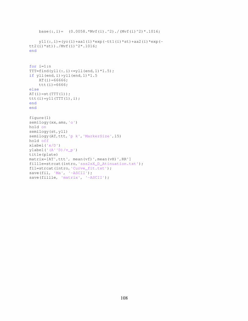
108
base(:,i)= (0.0058.*Mvf(i).^2)./(Mvf(i)^2)*.1016; yll(:,i)=(yo(i)+aa1(i)*exp(-tt1(i)*st)+aa2(i)*exp(-tt2(i)*st))./Mvf(i)^2*.1016; end for i=1:n TTT=find(yll(:,i)<=yll(end,1)*1.5); if yll(end,i)>yll(end,1)*1.5 AT(i)=66666; ttt(i)=6666; else AT(i)=st(TTT(1)); ttt(i)=yll(TTT(1),i); end end figure(1) semilogy(xx,ams,'o') hold on semilogy(st,yll) semilogy(AT,ttt,'p k','MarkerSize',15) hold off xlabel('x/D') ylabel('(A''D)/v_p') title(plate) matrix=[AT',ttt', mean(vf)',mean(vH)',RR'] fillle=strcat(intro,'sss2sX_D_Atinuation.txt'); fil=strcat(intro,'Curve_fit.txt'); save(fil, 'Ma', '-ASCII'); save(fillle, 'matrix', '-ASCII');