experimental characterization of flow induced vibration in
TRANSCRIPT

Brigham Young University Brigham Young University
BYU ScholarsArchive BYU ScholarsArchive
Theses and Dissertations
2009-08-12
Experimental Characterization of Flow Induced Vibration in Experimental Characterization of Flow Induced Vibration in
Turbulent Pipe Flow Turbulent Pipe Flow
Andrew S. Thompson Brigham Young University - Provo
Follow this and additional works at: https://scholarsarchive.byu.edu/etd
Part of the Mechanical Engineering Commons
BYU ScholarsArchive Citation BYU ScholarsArchive Citation Thompson, Andrew S., "Experimental Characterization of Flow Induced Vibration in Turbulent Pipe Flow" (2009). Theses and Dissertations. 1906. https://scholarsarchive.byu.edu/etd/1906
This Thesis is brought to you for free and open access by BYU ScholarsArchive. It has been accepted for inclusion in Theses and Dissertations by an authorized administrator of BYU ScholarsArchive. For more information, please contact [email protected], [email protected].

EXPERIMENTAL CHARACTARIZATION OF FLOW INDUCED
VIBRATION IN TURBULENT PIPE FLOW
by
Andrew S. Thompson
A thesis submitted to the faculty of
Brigham Young University
in partial fulfillment of the requirements for the degree of
Master of Science
Department of Mechanical Engineering
Brigham Young University
December 2009


Copyright © 2009 Andrew S. Thompson
All Rights Reserved


BRIGHAM YOUNG UNIVERSITY
GRADUATE COMMITTEE APPROVAL
of a thesis submitted by
Andrew S. Thompson This thesis has been read by each member of the following graduate committee and by majority vote has been found to be satisfactory. Date R. Daniel Maynes, Chair
Date Jonathan D. Blotter
Date
Julie Vanderhoff


BRIGHAM YOUNG UNIVERSITY As chair of the candidate’s graduate committee, I have read the thesis of Andrew S. Thompson in its final form and have found that (1) its format, citations, and bibliographical style are consistent and acceptable and fulfill university and department style requirements; (2) its illustrative materials including figures, tables, and charts are in place; and (3) the final manuscript is satisfactory to the graduate committee and is ready for submission to the university library. Date R. Daniel Maynes
Chair, Graduate Committee
Accepted for the Department
Larry L. Howell Graduate Coordinator
Accepted for the College
Alan R. Parkinson Dean, Ira A. Fulton College of Engineering and Technology


ABSTRACT
EXPERIMENTAL CHARACTARIZATION OF FLOW INDUCED
VIBRATION IN TURBULENT PIPE FLOW
Andrew S. Thompson
Department of Mechanical Engineering
Master of Science
This thesis presents results of an experimental investigation that characterizes the
wall vibration of a pipe with turbulent flow passing through it. Specifically, experiments
were conducted using a water flow loop to address three general phenomena. The topics
of investigation were: 1) How does the pipe wall vibration depend on the average flow
speed, pipe diameter, and pipe thickness for an unsupported pipe? 2) How does the
behavior change if the pipe is clamp supported at various clamping lengths? 3) What
influence does turbulence generation caused by holed baffle plates exert on the pipe
response?
A single pipe material (PVC) was used with a range of internal diameters from
5.08 cm to 10.16 cm and diameter to thickness ratios ranging from 8.90 to 16.94. The


average flow speed that the experiments were conducted at ranged from 0 to 11.5 m/s.
Pipe vibrations were characterized by accelerometers mounted on the pipe wall at several
locations along the pipe length. Rms values of the pipe wall acceleration and velocity time
series were measured at various flow speeds. Power spectral densities of the
accelerometer data were computed and analyzed. Concurrent wall pressure fluctuation
measurements were also obtained.
The results show that for a fully developed turbulent flow, the rms of the wall
pressure fluctuations is proportional to the rms of the wall acceleration and each scale
nominally as the square of the average fluid velocity. Also, the rms of the pipe wall
acceleration increases with decreasing pipe wall thickness. When changes were made in
the pipe support length, it was observed that, in general, pipe support length exercises
little influence on the pipe wall acceleration. The influence of pipe support length on the
pipe wall velocity is much more pronounced. A non-dimensional parameter describing
the pipe wall acceleration is defined and its dependence on relevant independent non-
dimensional parameters is presented.
Turbulence was induced using baffle plates with various sizes (2.54 cm to 0.159
cm) and numbers of holes drilled through them to provide a constant through area of
35.48 cm2 for each plate. Cavitation exists at high speeds for the largest holed baffle
plates and this significantly increases the rms of the pipe wall acceleration. As the baffle
plate hole size decreases, vibration levels were observed to return to levels that were
observed when no baffle plate was employed. Power spectral densities of the
accelerometer data from each baffle plate scenario were also computed and analyzed.


ACKNOWLEDGMENTS
I came to Dr. Daniel Maynes as a physics undergraduate student to advise me as I
completed my final project. While working with him, Dr. Maynes informed me of this
project and that he was looking for a prospective graduate student to work on it. I
accepted and have thoroughly enjoyed what I have been able to learn through the course
of completing this thesis. I would like thank to Dr. Maynes for giving me this
opportunity. And also for essentially giving me the reigns of this work; which, under his
guidance, allowed me to gain knowledge, experience, and confidence that I would not
have been able to gain any other way.
I would also like to thank Dr. Jonathan Blotter for adding his time, direction,
expertise, and equipment which also made it possible to complete this project and to
understand what some of the data were saying. To Dr. Julie Vanderhoff, thank you for
being willing to be a part of my committee when I just asked out of the blue. Also, I
would like to thank Genscape Inc. and Control Components Inc. for their interest in this
project and for the funding that made it possible.
Finally, I would like to thank my wife Nicole for the patience and love she has
given me as I have completed my thesis. She has always been very supportive of my
endeavors and I do not think I could have succeeded without her encouragement.


ix
TABLE OF CONTENTS
LIST OF TABLES ......................................................................................................... xiii
LIST OF FIGURES ........................................................................................................ xv
1 Introduction ............................................................................................................... 1
1.1 Objective ............................................................................................................. 3
1.2 Hypothesis .......................................................................................................... 3
1.3 Scope and Thesis Outline ................................................................................... 4
2 Background ............................................................................................................... 7
2.1 External Turbulent Flow Past Cylinders ............................................................. 7
2.2 Internal Turbulent Pipe Flow .............................................................................. 9
2.2.1 Pipe Flow Characteristics ............................................................................... 9
2.2.2 Orifice Induced Vibrations ........................................................................... 13
2.3 Scaling Relations .............................................................................................. 15
2.4 Comparison of Scaling Relations to Experimental Data .................................. 18
2.5 Contributions .................................................................................................... 23
3 Experimental Facility ............................................................................................. 25
3.1 Water Flow Loop .............................................................................................. 25
3.2 Test Sections ..................................................................................................... 28
3.3 Instrumentation ................................................................................................. 34
3.4 Measurement Error Analysis ............................................................................ 36

x
3.4.1 Pressure Fluctuation Uncertainty Analysis ................................................... 36
3.4.2 Accelerometer Uncertainty Analysis ............................................................ 38
3.5 Data Acquisition ............................................................................................... 38
3.6 Experimental Process ........................................................................................ 39
4 Results ...................................................................................................................... 43
4.1 Unsupported Pipe .............................................................................................. 43
4.1.1 Wall Pressure Fluctuations ........................................................................... 44
4.1.2 Accelerometer Measurements ....................................................................... 48
4.2 Pipe Wall Supports ........................................................................................... 60
4.2.1 Pipe Vibration vs. Support Length for the 10.16 cm Schedule 40 Pipe ....... 60
4.2.2 Pipe Vibration for Varying Clamping Lengths and all Test Sections........... 64
4.2.3 Accelerometer Spectra for Varying L/D ....................................................... 69
4.3 Non-dimensionalization of A’ ........................................................................... 71
4.4 Baffle Plate Influence ....................................................................................... 86
4.4.1 Various Baffle Plate Sizes ............................................................................ 86
4.4.2 Accelerometer Spectra for Baffle Plate Scenarios ........................................ 97
5 Conclusion ............................................................................................................. 103
5.1 Vibration Dependence on Fluid Speed and Un-Supported Pipe Parameters .. 103
5.2 Vibration Dependence on Fluid Speed and Clamped Pipe Parameters .......... 104
5.3 Non-Dimensionalization of A’ ........................................................................ 105
5.4 Baffle Plate Influence on Pipe Response ........................................................ 105
5.5 Recommendations ........................................................................................... 106
5.6 Publications ..................................................................................................... 107
6 References .............................................................................................................. 109
Appendix A: MatLab rms Code .................................................................................. 111

xi
Appendix B: MatLab à Code ...................................................................................... 113
Appendix C: Pipe Scaling Estimations ....................................................................... 115

xii

xiii
LIST OF TABLES
Table 2-1: Pipe material, diameters, and wall thicknesses for data of Pittard, et al 3. ...........19
Table 3-1: Internal pipe diameters and wall thicknesses for experiments with PVC pipes. ..29
Table 3-2: Pressure error estimates based on tap hole size, tapping depth, and orifice edge. ...........................................................................................................................38
Table 3-3: List of experiments conducted. Where X's signify that an experiment was conducted at the listed conditions and O’s indicate no experiment. ..........................41
Table 4-1: Average of each of the six test section power law exponents, m, (A’ and V’ ~ Vf
m) for each of the three clamping support lengths (no clamping, full clamping, and quarter clamping). Also displayed is the standard deviation of m over the six test sections. ...............................................................................................................67
Table 4-2: The values of m corresponding to A*~ Z*m power law determined by a numerical simulation of flow induced pipe vibrations presented by Shurtz 24. .........73
Table 4-3: The values of m corresponding to A*~ Rem power law for each of the six test sections considered and the three clamping support lengths. ....................................77
Table 4-4: The value of m from a power law fit of the 2.54 cm, 0.635 cm, and 0.159 cm baffle plate data with x/D. ..........................................................................................92

xiv

xv
LIST OF FIGURES
Figure 1-1: Photograph of the ruptured pipe from the NTSB accident brief. The arrow indicates the rupture site 3. .......................................................................................... 1
Figure 2-1: -5/3 power law roll-off in inertial subrange of various turbulent flows. The horizontal axis represents the non-dimensional frequency and the vertical axis represents the non-dimensional PSD 13. .....................................................................11
Figure 2-2: Non-dimensionalized PSD 1.7 pipe diameters downstream from an orifice plate 17. .......................................................................................................................14
Figure 2-3: A' measured in m/s2 as a function of Vf (top panel) and Q (bottom panel) for flow through five pipes of varying material and diameter as shown in the figure legends. Data obtained from Pittard, et al. 2. .............................................................21
Figure 2-4: V' measured as a function of Vf (top panel) and Q (bottom panel) for flow through four pipes of varying material and diameter as shown in the figure legends. Data obtained from Pittard, et al. 3. .............................................................22
Figure 3-1: Schematic diagram of flow loop with callouts corresponding to photographs below. .........................................................................................................................30
Figure 3-2: Photograph of a vent column. .............................................................................31
Figure 3-3: Photographs of pump, bypass line, flow conditioner, 5.08 cm developing region and vent column. .............................................................................................31
Figure 3-4: Photograph of rubber couplers leading into the 5.08 cm diameter developing region. ........................................................................................................................32
Figure 3-5: Photograph of 10.16 cm and 5.08 cm test sections. Wall supports are shown in the background. ......................................................................................................32
Figure 3-6: Photograph of vibration isolation downstream of the 5.08 cm test section before re-expansion to 10.16 cm pipe. .......................................................................33
Figure 3-7: Baffle plates used for experiments with 2.54 cm (top left), 1.27 cm (top right), 0.635 cm (middle left), 0.318 cm (middle right) and 0.159 cm (bottom) holes. ..........................................................................................................................34

xvi
Figure 4-1: P' as a function of the total pressure drop, ΔP, across the test section for the Schedule 80 7.62 cm test section. ..............................................................................45
Figure 4-2: P' as a function of the average fluid speed, Vf (upper panel), and average flow rate, Q (lower panel), for flow through the six test sections. .....................................47
Figure 4-3: A' as a function of P' for flow through the six test sections. ...............................48
Figure 4-4: V' as a function of P' for flow through the six test sections. ...............................49
Figure 4-5: A' as a function of Vf at seven x/D locations along the length of the 10.16 cm schedule 40 test section. .............................................................................................50
Figure 4-6: A' as a function of Vf (top panel) and Q (bottom panel) for flow through the six test sections considered. .......................................................................................51
Figure 4-7: A' as a function of D/t at Vf ≈ 6.7 m/s for each the three diameter pipes considered. .................................................................................................................53
Figure 4-8: V' as a function of Vf (top panel) and Q (bottom panel) for flow through the six test sections considered. .......................................................................................54
Figure 4-9: PSD for 7.62 cm schedule 40 test section with flow at speeds of 3.08 and 4.96 m/s. Also included is a line indicating a -5/3 relationship and the natural pipe response for reference. ...............................................................................................56
Figure 4-10: PSD for 7.62 cm schedule 40 test section with flow at speeds of 8.05 and 10.78 m/s. Also included is a line indicating a -5/3 relationship and the natural pipe response for reference. .......................................................................................57
Figure 4-11: PSD for 7.62 cm schedule 40 and 80 test sections with average flow speeds of 10.78 m/s and 10.98 m/s, respectively. Also included is a line indicating a -5/3 relationship and the natural pipe response for reference. ..........................................58
Figure 4-12: PSD for the 5.08, 7.62, and 10.16 cm schedule 40 test sections at a flow speed of nominally 6.7 m/s. Each data set has been multiplied by 100 (5.08 cm test section), 0.1 (7.62 cm test section), and 1x10⁻³ (10.16 cm test section) to allow each data set to be delineated. ..........................................................................59
Figure 4-13: A' as a function of Vf for various wall support distances in the 10.16 schedule 40 test section. .............................................................................................61
Figure 4-14: A' as a function of L/D for four flow speeds in the 10.16 cm schedule 40 test section. The solid lines represent the trend in the data at Vf =6.73 and 3.51 m/s .......62
Figure 4-15: V' as a function of Vf for each pipe clamp length in the 10.16 cm schedule 40 test section. The solid lines illustrate how V' trends with Vf. .....................................63

xvii
Figure 4-16: V' as a function of L/D for four flow speeds in the 10.16 cm schedule 40 test section. The solid lines represent the trend in the data at Vf =6.73 and 3.51 m/s. .....64
Figure 4-17: A’ as a function of Vf for the D = 5.08 cm schedule 80 test section with D = 5.08 cm and 10.16 cm developing regions and for the unsupported pipe case. .........66
Figure 4-18: A’ vs. D/t at a flow speed of 6.70 m/s for each test section diameter (5.08 cm, 7.62 cm, and 10.16 cm) and the three clamping support lengths (no support, full support, quarter support). ....................................................................................68
Figure 4-19: Comparison of à vs. f for unsupported and quarter support 7.62 cm schedule 40 test sections with a flow speed of 10.78 m/s. The unsupported case has been multiplied by 1000 to make comparison easier. ........................................................70
Figure 4-20: A* vs. Re for each of the six test sections considered and for no clamping support. .......................................................................................................................74
Figure 4-21: A* vs. Re for each of the six test sections considered and for full clamping support. .......................................................................................................................75
Figure 4-22: A* vs. Re for each of the six test sections considered and for the quarter clamping support. .......................................................................................................76
Figure 4-23: A* vs. t* for the three pipe diameters for the unsupported pipe. The values of A* have been averaged over a range of Re where there was little variation in A*. ....78
Figure 4-24: A* vs. ρ* for the three pipe diameters for the unsupported pipe. The values of A* have been averaged over a range of Re where there was little variation in A*. ....79
Figure 4-25: A’ vs. Vf2/t for each of the six unsupported test sections considered. Linear
fit lines with zero intercept pass through the schedule 40 and 80 pipe section data for each diameter. .......................................................................................................81
Figure 4-26: A’ vs. Vf2/ρ*t* for each of the six unsupported test sections considered.
Linear fit lines with zero intercept pass through the schedule 40 and 80 pipe section data for each diameter test section. ................................................................82
Figure 4-27: A’ vs. Vf2/ρ*t* for the data presented by Pittard et al. 2. ...................................83
Figure 4-28: A’ vs. Vf2.12βD1.9 for each of the six unsupported test sections considered. ......84
Figure 4-29: A’ vs. Vf2.12βD1.9 for the data presented by Pittard et al. 2. ................................85
Figure 4-30: A' as a function of tbaffle/Dhole for various flow velocities in the 10.16 cm schedule 40 test section and each of the five baffle plates. .......................................88

xviii
Figure 4-31: A' vs. Vf at seven x/D locations along the test section length with the 2.54 cm baffle plate. A' for the test section with no baffle plate has been included for reference. ....................................................................................................................89
Figure 4-32: A' vs. Vf at seven x/D locations along the test section length with the 0.635 cm baffle plate. A' for the test section with no baffle plate has been included for reference. ....................................................................................................................91
Figure 4-33: A' vs. Vf at seven x/D locations along the test section length with the 0.159 cm baffle plate. A' for the test section with no baffle plate has been included for comparison. ................................................................................................................91
Figure 4-34: A’ vs. Vf at x/D = 3 for all five baffle plates. A’ for the no baffle plate case is included for comparison. ...........................................................................................93
Figure 4-35: A’ vs. Vf at x/D = 30 for all five baffle plates. A' for the no baffle plate case is included for comparison. ........................................................................................94
Figure 4-36: The decay of A' with x/D for each baffle plate case at a flow speed of 3.61 m/s. .............................................................................................................................95
Figure 4-37: The decay of A' with x/D for each baffle plate case at a flow speed of 6.84 m/s. .............................................................................................................................96
Figure 4-38: à at three x locations downstream of the 2.54 cm baffle plate at a flow speed of 2.12 m/s. The sets of à data have been multiplied by 1000 (x = 0.305 m), 1 (x = 3.05 m), and 0.01 (x = 5.79 m), respectively to differentiate the data sets. ...........98
Figure 4-39: à at three x locations downstream of the 2.54 cm baffle plate at a flow speed of 5.63 m/s. The sets of à data have been multiplied by 1000 (x = 0.305 m), 1 (x = 3.05 m), and 0.001 (x = 5.79 m), respectively to differentiate the data sets. .........98
Figure 4-40: à at a three x locations downstream of the 0.159 cm baffle plate at a flow speed of 2.12 m/s. Sets of à data have been multiplied by 1x10³ (x = 0.305 m), 1 (x = 3.05 m), and 1x10⁻³ (x = 5.79 m), respectively to differentiate the data sets. .. 100
Figure 4-41: à at a three x locations downstream of the 0.159 cm baffle plate at a flow speed of 5.63 m/s. sets of à data have been multiplied by 1x10⁴ (x = 0.305 m), 1 (x = 3.05 m), and 1x10⁻³ (x = 5.79 m), respectively to differentiate the data sets. .. 101
Figure 4-42: à at 0.305 m downstream of each of the five baffle plates and at a flow speed of 5.63 m/s. Sets of à data have been multiplied by 1x10⁵ (2.54 cm baffle), 1 x10³ (1.27 cm baffle), 1 (0.635 cm baffle), 1x10⁻⁴ (0.318 cm baffle), and 1x10-
7 (0.159 cm baffle), respectively to differentiate the data sets. ................................ 101
Figure 4-43: à at 5.79 m downstream of each of the five baffle plates and at a flow speed of 5.63 m/s. Sets of à data have been multiplied by 1x10⁵ (2.54 cm baffle),

xix
1 x10³ (1.27 cm baffle), 1 (0.635 cm baffle), 1x10⁻² (0.318 cm baffle), and 1x10-
5 (0.159 cm baffle), respectively to differentiate the data sets.
................................ 102

xx
1
1 Introduction
Conveying fluids through pipes has been a very important aspect of human
civilization for thousands of years. In recent decades transporting gas, water, oil and
other fluids has made many economic activities possible. However, in the U.S. about
60% of the pipelines have been in use for over 25 years and are becoming prone to
failure 1. One of the contributing sources of failure in pipe systems is loss of integrity
due to fatigue loading caused by excessive vibration 2. One example of this occurred on
January 27, 2000. At about 12:12 p.m. a Marathon Ashland pipe ruptured near
Winchester, Kentucky releasing 11,644 barrels of crude oil onto a golf course and into
nearby Two Mile Creek. A post-accident investigation determined that its probable
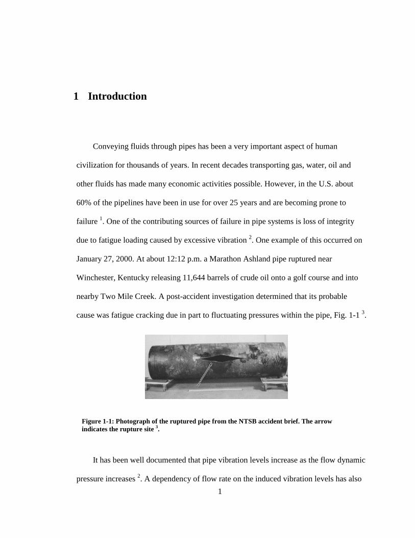
cause was fatigue cracking due in part to fluctuating pressures within the pipe, Fig. 1-1 3.
It has been well documented that pipe vibration levels increase as the flow dynamic
pressure increases 2. A dependency of flow rate on the induced vibration levels has also
Figure 1-1: Photograph of the ruptured pipe from the NTSB accident brief. The arrow indicates the rupture site 3.

2
been observed 2. Experimental and numerical techniques have been used by several
research groups to try to investigate this dependency with varying success. Although
each investigation has yielded different results, each has also concluded that pipe
vibration is a direct result of the inherent spatially and temporally varying pressure at the
pipe wall 2.
Although vibrations can lead to unwanted consequences, the monitoring of
vibration levels can also be used to provide non-intrusive flow sensing. Several types of
flow sensors have been developed over the centuries, with the earliest being developed
over 2100 years ago as simple siphon tubes attached to a constant head reservoir 4. More
modern flow sensors include, among others, orifice and venturi meters, flow nozzles,
vortex shedding meters, turbine meters, and Coriolis flow meters. These types of sensors
require interrupting the flow, which, for some applications, is not always possible. A
non-intrusive flow sensing technique has been expressed by several researchers and has
broad application throughout industry 2, 5, 6. As a specific example, Genscape Inc., a
provider of energy generation and transmission data to energy traders, power plant and
pipe line owners and operators, and regulatory agencies, monitors gas and oil flows
which help energy traders develop market/price forecasting models, determine supply
and demand tightness in regional markets, understand price drivers, and provide flow
data in U.S. pipelines 7. As a third party entity, it is not permissible for them to
potentially compromise a pipe’s structural integrity by installing and maintaining
intrusive flow sensors; so a non-intrusive flow sensing technique would allow them to
provide the necessary data to their customers without compromising the infrastructure.
Non-intrusive techniques could also be used to characterize the stresses and loading in a
3
piping system to predict catastrophic failures, such as the January 2000 accident, or
monitor the flow of corrosive substances that would quickly render an intrusive flow
sensor inoperable 2.
1.1 Objective
The objective of this research was to characterize the pipe wall vibrations caused
by fully-developed turbulent pipe flow. The influence of pipe diameter and thickness,
and pipe length was also explored. This was done by conducting an experimental study
that utilized pipe-wall mounted accelerometers and pressure transducers to determine the
relationship between these factors. Specifically, pressure fluctuation and vibration level
measurements were made in various diameters and thicknesses of PVC pipe with several
clamping support distances. Also, pipe vibration measurements due to different levels of
induced turbulence were conducted by inserting baffle plates into the flow field.
1.2 Hypothesis
It is clear that understanding how pipe vibration levels depend on flow dynamics
and pipe characteristics is important. According to other studies, the characteristic
vibration level, A’, which is defined as the standard deviation of the pipe acceleration
time series, can be expressed as 8:
A’ = f(Vf, D, t, L, ρf, ρp, E, …) (1-1)
Where Vf is the average fluid velocity, D is the internal pipe diameter, t is the pipe
thickness, L is the pipe length, ρf is the fluid density, ρp is the pipe density, and E is the

4
modulus of elasticity of the pipe. As previously stated, vibration levels have been
observed to increase with increased dynamic pressure (ρf Vf2). Because dynamic pressure
is a function of fluid velocity, it is expected that vibration levels will increase as the
square of the fluid velocity and flow rate. Because surface area increases with D, it is
also expected that vibration levels will increase as pipe diameter increases. As pipe
thickness decreases, it expected that vibration levels will increase because the pipe walls
should be able to respond more easily to changes in the local dynamic pressure. Because
changes in the pipe support length can affect the natural response of the pipe, it is
expected that this parameter will also affect the vibration levels, but will not have as
strong of an influence as the previously described parameters. Finally, because baffle
plates are designed to induce turbulence in the flow, they are expected to increase
vibration levels.
1.3 Scope and Thesis Outline
Pipe vibration levels were quantified for average fluid speeds ranging from 0 -11.5
m/s, with water as the working fluid. Flow through schedule 40 and 80 PVC pipe test
sections of diameters 5.08 cm -10.16 cm and diameter to thickness ratios ranging from
8.9 -16.9 were characterized. These results are compared to a similar study conducted at
Idaho State University. The effects on pipe vibration levels due to wall mounted clamp
supports of varying distances was also investigated. Finally, the effects of baffle plates of
varying hole size, inserted into the flow, was examined.
Because only one fluid and pipe material was examined in this study, dependency
of vibration levels on pipe density, fluid density, and pipe modulus of elasticity was not

5
addressed. Also, the range of available pipe diameters and thicknesses is limited to
standard sizes and one cannot be changed without also changing the other. Thus, the
individual influence of these two parameters individually is somewhat confounded.
The remainder of this thesis is organized as follows:
Chapter 2 contains a literature review and background information. It describes
how vibration levels are expected to scale with influential variables. Literature that
describes turbulent external flow past cylinders and of internal turbulent flow in pipes is
reviewed. Finally, the results of a similar study done at Idaho State University will be
summarized.
Chapter 3 details the experimental facility and experimental process.
Chapter 4 presents the results of the experiments performed.
Chapter 5 summarizes the conclusions of this research and discusses possible areas
of future research.

6

7
2 Background
This chapter details previous work that has been conducted to characterize flow
induced vibrations. First, a summary of work done on external turbulent flow past
cylinders is described. It will be seen that some of the results are applicable to internal
pipe flow and are discussed in Section 2.1. Next, work focusing on internal pipe flow will
be reviewed and is contained in Section 2.2. Section 2.3 considers how turbulence
induced pipe vibrations are expected to scale with flow and pipe characteristics. Finally,
section 2.4 will give a detailed review of a similar study done at Idaho State University.
2.1 External Turbulent Flow Past Cylinders
Related work, which has relevance in the nuclear power industry, has explored
external turbulent flow past cylindrical rods with the flow direction aligned with the rod
axis. In a work by Paidoussis 9, the behavior of cylinders in both cross flow and axial
flow are described. Paidoussis states that the behavior of an array of cylinders in cross
flow exhibit three main characteristics; first, at low flow velocities is responding chiefly
to turbulent buffeting; observing that as fluid velocity increases, the vibration level
increases as the fluid velocity squared. Then as the flow velocity continues to increase, a
peak develops as the cylinders respond to such phenomenon as vortex shedding and

8
resonance. Finally, as the flow velocity continues to increase, a fluid elastic instability
develops and the cylinders are expected to respond with large amplitude motions.
Turbulent fluid flow, which is made up of eddies of various sizes and energies,
coupled with the flow periodicity that results as a fluid moves around a cylinder set up
forced vibrations in the cylinder. These forced vibrations are made up of non-resonant
components that are present at all flow velocities and resonant components that exist in
the frequency band near the cylinders’ natural frequency. In the resonant frequency band,
the cylinders extract energy from the fluctuating pressure field near the cylinders 9.
Others 9 found that away from the resonant frequency band, the cylinders response was
proportional to the fluid velocity squared, as stated above.
Addressing axial flow around cylinders, Paidoussis states that vibrations observed
below the threshold of fluid elastic instabilities are also widely accepted to be caused by
pressure fluctuations in the flow field, similar to cylinders in cross flow. These pressure
fluctuations are made up of near and far field components with the near field consisting
of local pressure fluctuations associated with the boundary layer and the far field
consisting of acoustic disturbances. It is also shown that cylinders in axial flow respond
in a similar fashion to cylinders in cross flow, i.e., responding proportionally to the fluid
velocity squared except near the resonant frequency band and above the fluid elastic
instability.
In a work by Reavis 10, the author calculates the response of fuel elements in
parallel flow making use of experimental data from Burgreen et al. 10 and empirical
correlations derived via dimensional analysis of beam motion by Burgreen and

9
Paidoussis 10. The available data described the pressure fluctuations in a turbulent
boundary layer. Similar to the works described above, the fuel element’s response is
forced by the fluctuating pressure field in the turbulent boundary layer.
These previous works show that the vibration response of cylinders placed in
turbulent flow is due to the pressure fluctuations in the boundary layer. They also show
the vibration levels are proportional to the average fluid velocity squared. Though not
discussed in detail here, the correlations mentioned above include average fluid velocity,
rod diameter, fluid density, and mass per unit length of the rod as dependant variables10.
Similar factors are also expected to be important in turbulent flow through pipes.
2.2 Internal Turbulent Pipe Flow
2.2.1 Pipe Flow Characteristics
Fully developed turbulent pipe flow is made up of eddies and vortices of various
sizes, ranging from the same order of magnitude as the inner pipe diameter to the
Kolmogorov scale. The turbulent kinetic energy contained in the eddies increases with
flow velocity, resulting in greater pressure fluctuations 2. The largest eddies are the result
of whatever mechanism is responsible for the turbulence generation (i.e. wall shear, jets,
etc) 10. Here the transfer of energy is from the mean flow to the large eddies 2. These
large eddies are also the most energetic and transfer their energy into smaller eddies
which in turn transfer energy to smaller eddies, until dissipation takes place at the
Kolmogorov scale (the smallest turbulent length and time scales) 2, 10. This all takes place
within the boundary layer, which for fully developed pipe flow is across the entire inner
pipe diameter. Because these fluid packets have various amounts of kinetic energy, as

10
they approach the pipe wall the energy is converted into another form. Some portion is
converted into heat, but most of it is converted into pressure and pressure fluctuations, a
form of potential energy 5.
Calculating the power spectral density, PSD, of the turbulent field reveal structures
that are common for a wide range of turbulent flows. Figure 2-1 illustrates the spectral
decay in a region known as the inertial subrange (the red line) where E11 is the energy
spectrum function, k1 is wave number and is related to frequency by the fluid velocity, ε
is the rate of energy dissipation, ν is the kinematic viscosity, and η is the Kolmogorov
scale. As hypothesized by Kolmogorov, turbulent energy in the inertial subrange
cascades from large scales (low frequencies) to small scales (high frequencies) without
significant production or dissipation 12. In the inertial subrange, the wave number extent
increases with Reynold’s number and decays as k1η 13, 12, 14. Also, because wave number
is related to frequency (f) by the fluid velocity, the frequency extent in the inertial
subrange will decay as f-5/3. Although the -5/3 relationship is pervasive through turbulent
research, the cascade explanation has come with some criticism because among other
things the -5/3 law has never been able to be extracted from the Navier-Stokes equations
15. Even with arguments against it, the -5/3 relationship is supported experimentally in
many types of turbulent flows. It will be expected that for the results presented in this
thesis, there should also be a -5/3 roll-off in the PSD of the pipe vibrations, due to their
proportionality to the pressure fluctuations.

11
A work by Evans et al. 5 shows how the turbulence induced pipe vibrations relate
to the pressure fluctuations in the fluid for the purpose of developing a non-intrusive flow
sensing technique. The analysis by Evans et al.5 is based on a 1-D model of a beam in
bending. The result of this analysis demonstrates that the pipe vibrations are proportional
to the pressure fluctuations. Also demonstrated is that the square of the fluctuations in
flow rate are proportional to the pressure fluctuations, which leads to the implication that
Figure 2-1: -5/3 power law roll-off in inertial subrange of various turbulent flows. The horizontal axis represents the non-dimensional frequency and the vertical axis represents the non-dimensional PSD 13.
k1η-5/3
k1η
E11
(k1)
/(εν5
)1/4

12
the standard deviation of the pipe vibrations is proportional to the average flow rate
squared.
Utilizing the quadratic relationship between flow rate and pipe vibrations,
Awawdeh, et al. attempt to develop a sensor network to monitor changes in pipe flow
rate1. Using a wireless sensor network to collect data, accelerometers were attached to
10.82 cm inner diameter water conveying steel pipes. Time series vibration data were
collected at no flow and two other flow rates. It is shown that changes in flow rate can be
tracked non-invasively using accelerometers mounted on the pipe wall 1. The
experimental setup for this study did not describe vibration isolation of the test section
from other vibration sources and thus may be subject to other sources of signal noise.
Kim and Kim developed a method for measuring flow rate in a pipe by utilizing an
external exciter and three accelerometers 6. The accelerometers were placed equal
distances from each other along the length of 3 cm inner diameter, steel, water conveying
pipe. The pipe was excited with white noise up to 55 kHz with a shaker and the system
was run at four flow rates from 0 to 3.08 L/s. The effects of the moving internal fluid
through the shaker excited pipe caused a shift in the axial wave number (Doppler shift)
that was converted to flow rate. A Gaussian fit was applied to the histogram of each
measurement configuration at discrete frequencies and then compared to the histogram of
the actual flow rate, and it was found that the Gaussian fits coincided with the actual flow
rates within 12% uncertainty 6. The experimental setup used for this thesis differs from
the work done by Kim. Specifically, the pipe is not excited by white noise and the
accelerometers are not positioned as described by Kim. However, this thesis does show

13
that there is a coupling between internal pipe flow and pipe vibration that can be utilized
as a non-intrusive flow sensing technique.
2.2.2 Orifice Induced Vibrations
Large amplitude vibrations were observed in particular flow regimes in a French
nuclear power plant. These unwanted vibrations were attributed to cavitation induced by
single hole orifices. Conducting experiments to try to explain and reduce the large
amplitude pipe vibrations Caillaud et al. found that the vibrations were caused by
supercavitation at the orifice, significantly disturbing the flow 16.
Qing et al. studied orifice induced wall pressure fluctuations and pipe
vibrations17. The study was performed by mounting accelerometers and dynamic pressure
transducers before and after an orifice plate to measure structural vibrations and wall
pressure fluctuations. The pipe was 9.0 cm internal diameter stainless steel, and three
orifice plates were used, with orifice diameters of 2.3 cm, 2.74 cm, and 3.02 cm (a no
orifice plate condition was also used). Three flow rates were investigated, which
translated into flow speeds of 0.65 m/s, 0.87 m/s and 1.09 m/s. The root mean square
(rms) and power spectral density (PSD) of the pressure measurement time series were
then calculated. It was found that without an orifice plate the rms of the pressure
fluctuations remained nearly the same at each measurement point. Adding an orifice plate
results in a sharp rise in the rms values of the fluctuating pressure, indicating that the
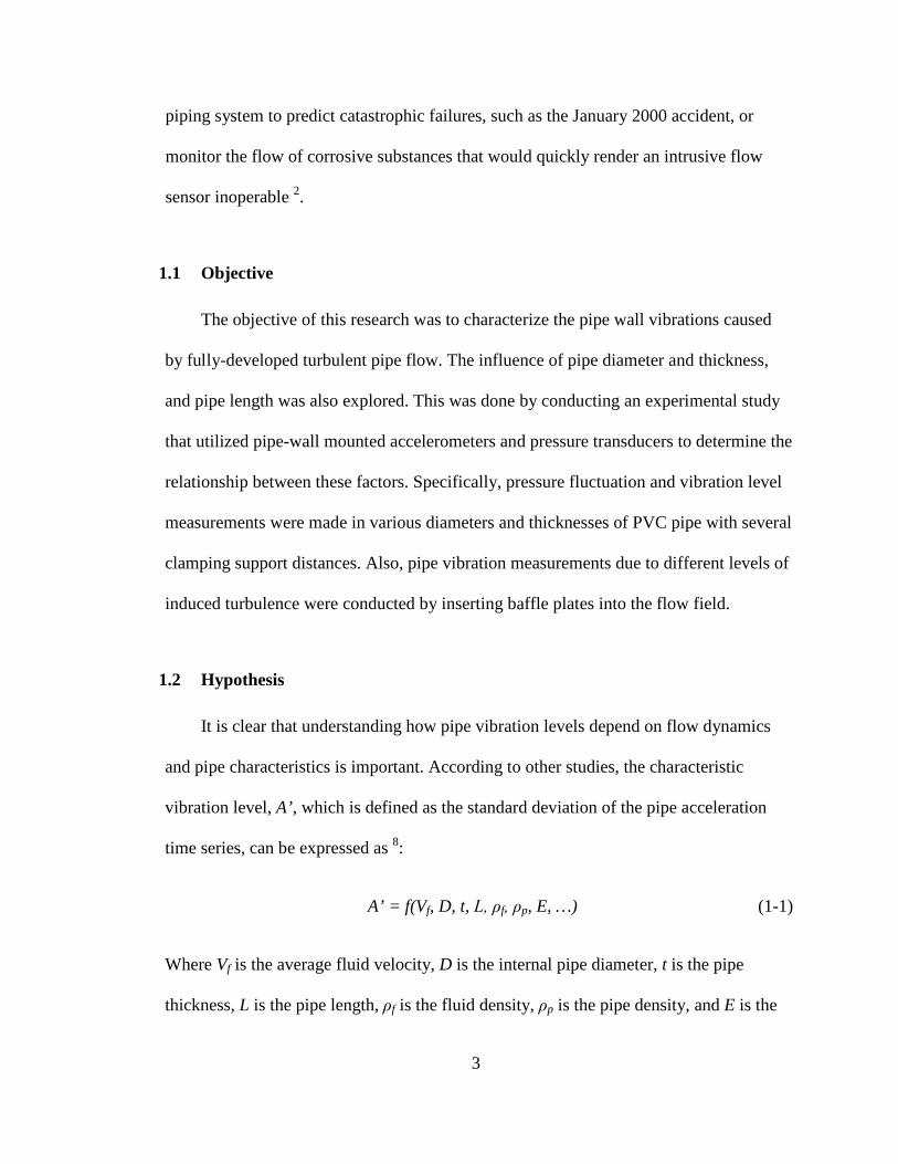
flow is significantly disturbed by the orifice plates. Figure 2-2 illustrates the non-
dimensionalized PSD vs. Strouhal number (St = fD/Vf, where f is frequency, D is inner
pipe diameter, and Vf is fluid velocity) 1.7 pipe diameters downstream from the 3.02 cm
14
orifice, where the maximum pressure fluctuations were observed to occur. As the flow
passes through the orifice, the flow contracts and re-expands downstream. An eddy was
found to appear on the backside of the orifice due to cavitation. The PSD shows that the
flow’s energy content is below 400 Hz, St ≈ 6.2, and is concentrated below 71 Hz, St ≈
1.1. Further downstream less energy is concentrated in this low frequency range, and the
rms drops to nearly the same level as the no orifice condition, indicating that the orifice
disturbance is localized to the vicinity of the orifice plate 17.
The goal of a subsequent work by Qing was to develop empirical equations of the
fluctuating pressure PSD 18. The results conclude that cavitation can be avoided by
increasing the hole size of the orifice plate, but the induced pressure fluctuations, which
stimulate pipe vibration, cannot be eliminated. Also, the near field turbulence caused by
the localized disturbance affects the flow up to six pipe diameters downstream. Finally,
pressure fluctuations increase as flow rate increases or as the diameter of the orifice hole
decreases 18.
Figure 2-2: Non-dimensionalized PSD 1.7 pipe diameters downstream from an orifice plate 17.

15
In contrast to the works by Qing et al. 17, 18, in this thesis baffle plates with multiple
holes were used to induce turbulence over a significantly larger range of flow speeds and
multiple pipe diameters. It is expected however, that cavitation will be caused by the
baffle plates and that pressure fluctuations, and by extension pipe vibrations, will increase
dramatically. It is also expected that the PSD will behave in a similar fashion to Fig. 2-2,
with the majority of the energy below 400 Hz.
A study by Moussou provided an estimation of the vibrations of a water conveying
pipe subjected to orifice plate induced turbulent excitations 19. It was shown that the
cavitation induced vibrations can be directly identified by plotting the dimensionless pipe
vibration PSD. Specifically, cavitation adds a broad increase to the spectrum with an
amplitude that depends on the incipient cavitation 19. This localized increase may be
similar to the hump observed in Fig. 2-2 and is expected in the baffle plate experiments
performed for this thesis.
2.3 Scaling Relations
Evans showed that the standard deviation of the pipe vibrations scaled as the
standard deviation of the pressure fluctuations (A’ ~ P’) 5. It was also stated that kinetic
energy in the flow was converted into dynamic pressure near the wall. Referring to the
definitions of kinetic energy and dynamic pressure respectively:
𝐸𝐸𝑘𝑘~12𝑚𝑚𝑉𝑉𝑓𝑓2 (2-1)

16
𝑃𝑃~12𝜌𝜌𝑉𝑉𝑓𝑓2 (2-2)
in the above expressions m is mass, Vf is fluid velocity, and ρ is fluid density. The
dynamic pressure has units of kinetic energy per unit volume and it would be expected
that the dynamic pressure fluctuations of the flow are proportional to the kinetic energy
which goes as Vf2, implying that A’ ~ Vf
2.
Contained in Appendix C is a document by Maynes 20 that presents a scale
analysis of turbulence induced pipe vibration in a straight pipe for both the pipe bending
and expansion modes. The portion describing the scaling of the bending mode of pipe
vibration is summarized here for convenience.
Because turbulent pipe flow induces pressure fluctuations at the pipe wall, these
pressure fluctuations can be thought of as a loading function which causes deflection
fluctuations in an elastic beam. The standard deviation of the deflection fluctuations (δ’)
should scale as
𝛿𝛿′~
𝐹𝐹′𝐿𝐿3
𝐸𝐸𝐸𝐸 (2-3)
With the unsteady loading represented by F’, L is the pipe length between supports, E is
the modulus of elasticity, and I is the area moment of inertia. The loading F’ should scale
with P’ multiplied by a characteristic area, D2, where D is the inner pipe diameter.
Further, P’ should scale as the flow dynamic pressure as defined in Eq. 2-2. Substituting
this relationship into Eq. 2-3 gives

17
𝛿𝛿′~
𝜌𝜌𝑉𝑉𝑓𝑓2𝐷𝐷2𝐿𝐿3
𝐸𝐸𝐸𝐸 (2-4)
Fluctuations in the velocity of the pipe wall are expected to scale as δ’ (Eq. 2-4)
multiplied by the natural frequency of vibration of a pipe given by
𝜔𝜔𝑛𝑛~
1𝐿𝐿2�𝐸𝐸𝐸𝐸𝑚𝑚
(2-5)
Where m is the mass per unit length of the contained fluid and of the pipe, m = ρA+mpipe,
and A is the internal cross sectional area of the pipe. Multiplying Eq. 2-4 by Eq. 2-5 gives
the scaling relationship for the pipe velocity fluctuations, Vp’
𝑉𝑉𝑝𝑝′~
⎝
⎛𝑉𝑉𝑓𝑓2
�𝐸𝐸𝜌𝜌⎠
⎞��𝛽𝛽� �𝐷𝐷𝐿𝐿√𝐸𝐸� (2-6)
Here β is the ratio of fluid mass per unit length to total mass per unit length of the
combined fluid and pipe defined as
𝛽𝛽 =1
1 +𝜌𝜌𝑝𝑝𝜌𝜌 �4𝑡𝑡
𝐷𝐷 �1 + 𝑡𝑡𝐷𝐷��
(2-7)
t is the pipe wall thickness and ρp is the density of the pipe material. By inspection, it can
be seen that β scales to the first order as D/t. Finally, multiplying Eq. 2-6 by Eq. 2-5 gives
the fluctuations of pipe wall acceleration A’
𝐴𝐴𝑝𝑝′ ~
𝑉𝑉𝑓𝑓2𝛽𝛽𝐿𝐿
(2-8)

18
A similar scale analysis for the expansion modes yields 21
𝐴𝐴𝑝𝑝′ ~
𝑉𝑉𝑓𝑓2𝛽𝛽𝐷𝐷
(2-9)
The analysis suggests that δ’, V’, and A’ should scale with Vf2 for both modes
considered. As stated in Chapter 1 the influence of changing only pipe diameter without
changing any other parameters is not possible, but Eqs. 2-8 and 2-9 suggest that A’
should scale with β and V’ should scale as�𝛽𝛽. The relations presented here will be
compared to the experimental results of Pittard et al. in the next section.
2.4 Comparison of Scaling Relations to Experimental Data
Pittard et al. presented results of a study intended to explore the strong correlation
between flow rate and measured pipe vibration 2. The experimental portion of the study
was done at Idaho State University (ISU) using a flow loop similar to the one that will be
described in Chapter 3. Experiments were conducted in pipes of three different materials;
PVC, aluminum, and stainless steel. A description of these pipe sections is contained in
Table 2-1. Accelerometers were placed on the pipe wall and the standard deviation of the
frequency averaged time series was measured at various flow rates. A characteristic of
the ISU study that differentiates it from what will be presented in this thesis is that
different pipe materials were used with a wide range of pipe densities (1400, 2200, and
7800 kg/m3 for PVC, aluminum and stainless steel respectively) and moduli of elasticity
(2.9,70, and 200 GPa respectively). Flow rates ranged from 0.0033 m3/s to 0.025 m3/s,
resulting in a range of velocities from 0.4 m/s to 13.3 m/s.

19
Figure 2-3 shows the standard deviation of the pipe vibration measured by an
accelerometer, A’, as a function of Vf (top panel) and average flow rate, Q, (bottom panel)
and Fig. 2-4 shows the standard deviation of the pipe velocity, V’, as a function of Vf (top
panel) and Q (bottom panel) 3. The results shown in these two figures suggest a power
law dependence of A’ and V’ on Vf (i.e. Z’~Vfm, where Z’ represents the respective
variable of interest). A statistical analysis of the data reveals that for the A’ data, m varies
between 1.90 and 2.30 with an average of 2.16. This value is slightly greater (~8%) than
the quadratic relationship predicted by Eqs. 2-8 and 2-9 2. For V’, m varies from 1.61 to
1.75 with an average of 1.68. The values of m are the same when the data are plotted
versus Q. Figures 2-3 and 2-4 also give a limited characterization of the combined
influence of D/t. Specifically, the magnitude of A’ when plotted as a function of Vf is
greater for the 10.16 cm PVC than for the 7.62 cm PVC pipe sections. This is also
evident in the 7.62 and 3.81 cm stainless steel sections. This relationship is reversed
when A’ is plotted as a function of Q.
The data shown in Figs. 2-3 and 2-4 also suggest that the pipe vibration exhibit
only a very modest dependence on the pipe material properties, ρp and E. The data in the
Table 2-1: Pipe material, diameters, and wall thicknesses for data of Pittard, et al 3.
Pipe Section
Material D(m) t(m) D/t
10.16 cm Sch
PVC 0.102 0.00602 16.94 7.62 cm Sch
PVC 0.0779 0.00548 14.22 7.62 cm Sch
Aluminum 0.0779 0.00548 14.22 7.62 cm Sch
Stainless
0.0779 0.00548 14.22 3.81 cm Sch
Stainless
0.041 0.00368 11.14

20
figures show only small variations between the 7.62 cm PVC, aluminum, and stainless
steel pipe sections. The general trend shown in the data is that A’ increases only modestly
with decreased pipe density and/or modulus. An analysis done by Evans et al. 12 on the
same pipe diameters and materials show that the properties of the pipe materials change
the slope of A’ when plotted vs. Q. Specifically, as ρp and E increase, the slope of the A’
curve is observed to decrease modestly. It is also indicated that the D dependence is not
constant over the range of Q.
It is expected that the data presented in Chapter 4 will behave in a fashion similar
to the data acquired at ISU. Specifically P’ and A’ are expected to scale with Vf2 and V’ is
expected to scale nominally with Vf1.6. Also, A’ is expected to decrease as D increases
when plotted as a function of Vf.
To summarize, the literature reviewed above concludes that vibrations of
cylindrical rods placed in turbulent flow are due to fluctuating pressure loading. For
internal pipe flow, the PSD of the turbulence energy decays as frequency to the -5/3
power in the inertial subrange. P’ is proportional to A’ which also scales as Vf2 and this
general relationship makes it possible to predict flow rate by measuring the pipe
vibrations. It was also noted that A’ decreases as D increases over the range of flow rates
previously explored. Finally, the presence of an orifice plate produces turbulent
disturbances that cause significant increases in A’ and P’.

21
Figure 2-3: A' measured in m/s2 as a function of Vf (top panel) and Q (bottom panel) for flow through five pipes of varying material and diameter as shown in the figure legends. Data obtained from Pittard, et al. 2.
0.002
0.02
0.2
0.3 3
A' (m
/s2 )
Vf (m/s)
D = 7.62 cm PVC D = 10.16 cm PVCD = 7.62 cm AluminumD = 7.62 cm Stainless SteelD = 3.81 cm Stainless Steel
0.001
0.01
0.1
0.001 0.01
A' (m
/s2 )
Q(m3/s)
D = 7.62 cm PVC D = 10.16 cm PVCD = 7.62 cm AluminumD = 7.62 cm Stainless SteelD = 3.81 cm Stainless Steel
D = 7.62 cm PVC D = 10.16 cm PVC D = 7.62 cm Aluminum D = 7.62 cm Stainless Steel D = 3.81 cm Stainless Steel
D = 7.62 cm PVC D = 10.16 cm PVC D = 7.62 cm Aluminum D = 7.62 cm Stainless Steel D = 3.81 cm Stainless Steel

22
Figure 2-4: V' measured as a function of Vf (top panel) and Q (bottom panel) for flow through four pipes of varying material and diameter as shown in the figure legends. Data obtained from Pittard, et al. 3.
7.00E-06
7.00E-05
7.00E-04
0.3 3
V' (m
/s)
Vf (m/s)
D = 7.62 cm PVC
D = 10.16 cm PVC
D = 7.62 cm Aluminum
D = 7.62 cm Stainless Steel
7.00E-06
7.00E-05
7.00E-04
0.002 0.02
V' (m
/s)
Q(m/s)
D = 7.62 cm PVC
D = 10.16 cm PVC
D = 7.62 cm Aluminum
D = 7.62 cm Stainless Steel
D = 7.62 cm PVC D = 10.16 cm PVC D = 7.62 cm Aluminum
D = 7.62 cm Stainless Steel
D = 7.62 cm PVC
D = 7.62 cm PVC
D = 7.62 cm PVC
D = 7.62 cm PVC
23
2.5 Contributions
This work will result in the following contributions:
1. The dependency between wall acceleration (A’) and wall surface pressure
fluctuations (P’) will be determined by direct measurement of each parameter.
2. rms values of the pipe wall acceleration and velocity will be characterized over a
wide range of water speeds (0-11.5 m/s) and will provide greater understanding
of the dependence of each of these parameters on the average flow speed.
Previous studies have generally only focused on pipe wall acceleration.
3. The dependency of pipe diameter and thickness will be explored by considering
flow through six pipes (5.08 cm, 7.64 cm, and 10.16 cm Schedule 40 and 80
pipes). The number of pipe sizes is larger than most previous studies and will
provide greater understanding of the dependence of the rms values of the pipe
wall acceleration and velocity on the pipe diameter and wall thickness.
4. The influence of varying the clamping length of the pipes of interest on the pipe
acceleration will be characterized by conducting experiments with the pipes
clamped at discreet points.
5. The influence of baffle plates of varying hole size on the vibration levels will be
characterized using five different baffle plates. Although previous researchers
have explored orifice plates, the vibration levels caused by systematically
designed baffle plates has not previously been characterized.

24
A single pipe material (PVC) and fluid (water) was utilized in the experiments and
consequently the dependence of pipe material and fluid density on the vibration levels is
not possible. However, the amount of new data represents a significant contribution to the
body of knowledge for turbulent flow through pipes with and without baffle plates. The
results have applicability to both non-intrusive flow sensing and to design of pipe
systems to withstand the fatigue loading they will encounter.

25
3 Experimental Facility
This chapter describes the hardware and data acquisition processes that were used
to complete the experimental investigation. Sections 3.1 and 3.2 describe the components
of the flow loop and test sections respectively. Sections 3.3 to 3.5 detail the
instrumentation, measurement error analysis, and data acquisition hardware. Lastly,
section 3.6 details how the experiments were conducted.
3.1 Water Flow Loop
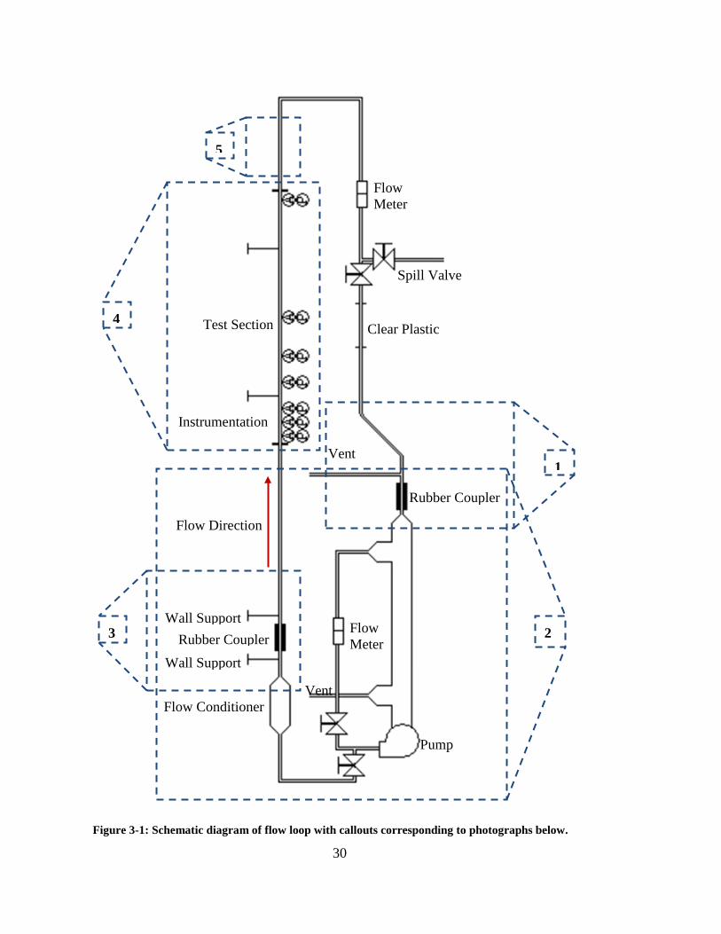
Experiments were conducted in a water flow loop constructed for that purpose
and is shown schematically in Fig. 3-1. Figures 3-2 to 3-6 are images of various portions
of the facility and are described further in the following text. Water was circulated
through the loop via a Bell and Gossett centrifugal pump with a maximum speed of 1800
RPM, driven by a 75 hp Marathon Electric 365T motor. The pump was placed on a
concrete pad to help isolate its vibrations from the rest of the room. The pump speed was
controlled by a Hitachi L300P 55kW, 75 hp variable frequency drive. The loop was filled
by two open vertical vent columns shown in Figs. 3-2 and 3-3. These columns extend
above the level of the flow loop to keep the system pressurized to approximately 3 kPa at
no flow and prevent air from leaking into the system. These columns also served to vent
entrained air bubbles resulting from the filling process and to prevent cavitation by

26
maintaining nearly atmospheric pressure at the pump inlet and near bends where low
pressure regions tend to develop.
The pump inlet is fed by 20.32 cm diameter schedule 80 PVC pipe (see Fig. 3-1
and Fig. 3-3). The pump outlets to 10.16 cm diameter schedule 80 pipe, which divides
into a bypass branch and a main branch. Each branch is controlled by hand-actuated gate
valves. The bypass line is a common fixture throughout the literature, providing a way to
control flow rate without changing pump speed, but was not used for this research.
After the bypass branch junction, the main line then expands to 20.32 cm
schedule 80 PVC to accommodate a flow conditioner (shown in Fig. 3-3) which
minimizes swirl and breaks up pump-induced turbulence. The flow conditioner consists
of a 7.62 cm thick piece of aluminum honeycomb caged between two cruciform
aluminum rings; between the honeycomb and the downstream cruciform ring is a layer of
PVC coated fiberglass mesh. Downstream of the second cruciform ring is another layer
of fiberglass mesh and two more aluminum rings each with a layer of fiberglass mesh
between them which provides for two more layers of fiberglass mesh. The rings and
mesh are bolted together as a single unit. This robust design prevents the aluminum
honeycomb from collapsing and being pushed through the flow loop when the flow rate
is high.
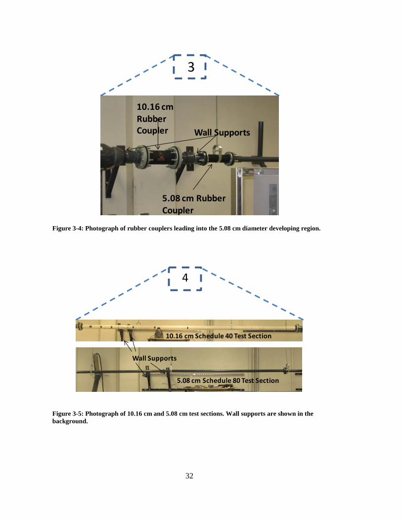
After the flow conditioner, the pipe contracts to 10.16 cm schedule 80 pipe. After
the contraction the pipe is connected to a flexible rubber coupler, Proco series 310
expansion joint. The coupler reduces structural vibrations transmitted to the test section
from the pump and pipe components and is connected to the building by two wall mounts

27
(one up-stream and one down-stream) to absorb low frequency pipe swaying. This
arrangement is shown in Fig. 3-4.
The flow then either enters a 10.16 cm diameter, 6.096 m long developing region
with a length to inner pipe diameter (L/D ~ 62) or is further reduced down to 5.08 cm
diameter schedule 80 and passes into another rubber coupler and then into a 3.35 m long
developing region of 5.08 cm schedule 80 pipe (L/D ~ 68). The developing regions allow
the flow to become fully developed before entering the test section. Figures 3-2 to 3-6
show the 5.08 cm diameter configuration of the flow loop. A typical correlation for the
development length for turbulent pipe flow is: 21
𝐿𝐿𝑒𝑒𝐷𝐷
= 4.4𝑅𝑅𝑒𝑒16 (3-1)
where Le/D is the ratio of entrance (developing) length to pipe diameter, and Re is the
Reynold’s number defined by:
𝑅𝑅𝑒𝑒 =𝜌𝜌𝑉𝑉𝑓𝑓𝐷𝐷𝜇𝜇
(3-2)
where ρ is the fluid density, D is the inner pipe diameter, and μ is the dynamic fluid
viscosity. According to Eq. 3-1, and for the largest Re explored in this study (Re ~106),
Eq. 3-1 yields Le/D ~ 44 indicating that the developing regions are more than sufficiently
long enough to allow the flow to become fully developed.
After the developing region, the flow then passes into a test section, shown in Fig.
3-5, which is described in further detail in section 3.2. After the 5.08 cm test sections, the
flow passes through a 1.22 m long segment of 5.08 cm schedule 80 pipe and another 5.08

28
cm diameter rubber coupler before re-expanding to 10.16 cm schedule 80 pipe. The 1.22
m long section provides for an L/D of 24 before the re-expansion to prevent disturbances
induced by the re-expansion from propagating back up-stream (see Fig. 3-6). Data were
taken using the 5.08 cm test sections with both the 10.16 cm developing region and the
5.08 cm developing region; the results will be discussed and compared in Chapter 4.
After the test section, the flow then passes into 10.16 cm schedule 80 pipe and returns to
the pump. On the return portion of the flow loop, a clear section of schedule 40 PVC is
mounted in line to allow visual inspection of the flow and to ensure that air entrainment is
not occurring.
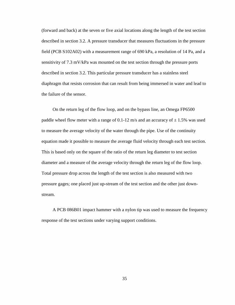
3.2 Test Sections
The test sections consist of long interchangeable sections of 5.08 cm, 7.62 cm, and
10.16 cm diameter schedule 40 and 80 PVC pipe (see Fig. 3-5). For the 10.16 cm and
7.62 cm diameter test sections, the developing region diameter was 10.16 cm. For the
5.08 cm diameter test section, both the 10.16 cm and 5.08 cm diameter developing
regions were used because there was concern that reducing from the 10.16 cm diameter
developing region to the 5.08 cm diameter test section would cause pipe vibrations
unrelated to this study. It was found that there was little difference between developing
regions and this result is discussed further in Chapter 4. The actual pipe internal
diameters, D, and wall thicknesses, t, of each test section are shown in Table 3-1. The test
sections are hung supported from ceiling mounts using flexible cables that are free to
swing. Along the wall adjacent to the test section are supports that can anchor each test

29
section to the wall, allowing the investigation of how pipe vibration varies with clamping
length.
A 0.159 cm hole was drilled into each test section at various axial locations along
the test section length. PVC ports with a 0.635 cm tapped through hole were then glued
onto the outside of the pipe at these locations to provide material to mount the pressure
transducers (discussed in section 3.3). These ports can be seen as the dark rectangles in
the photograph of the 10.16 cm schedule 40 test section (Fig. 3-5). Similar ports are
employed on all of the other test sections. For the test sections associated with the 10.16
cm diameter developing region, the ports were located at 0.305 m, 0.610 m, 0.914 m,
1.524 m, 2.134 m. 3.048 m, and 5.791 m from the flange at the entrance of the test
section. Accelerometers were also mounted at these same locations. The ports in the test
sections associated with the 5.08 cm test section were located 0.305 m, 0.610 m, 1.219 m,
1.829 m, 2.743 m, and 5.486 m from the flange at the entrance of the test section.
Table 3-1: Internal pipe diameters and wall thicknesses for experiments with PVC pipes.
Pipe Schedule D (m) t (m) D/t
5.08 cm Sch 80 0.0493 0.00554 8.899
7.62 cm Sch 80 0.0737 0.00762 9.672
10.16 cm Sch 80 0.0972 0.00856 11.355
5.08 cm Sch 40 0.0525 0.00391 13.427
7.62 cm Sch 40 0.0779 0.00548 14.215
10.16 cm Sch 40 0.102 0.00602 16.944
30
Figure 3-1: Schematic diagram of flow loop with callouts corresponding to photographs below.
Pump
Rubber Coupler
Vent
Vent
Flow Meter
Clear Plastic
Flow Meter
Spill Valve
Test Section
Instrumentation
Rubber Coupler Wall Support
Wall Support
Flow Conditioner
Flow Direction
3
4
5
1
2

31
Figure 3-2: Photograph of a vent column.
Figure 3-3: Photographs of pump, bypass line, flow conditioner, 5.08 cm developing region and vent column.
Vent Column
Rubber Coupler (10.16 cm)
Ceiling Supports
1
5.08 cm developing region
Flow Conditioner
Bypass Loop
Variable Speed Controller
Pump
Concrete Isolation Pad
Vent Column
Pump Inlet
2
32
Figure 3-4: Photograph of rubber couplers leading into the 5.08 cm diameter developing region.
Figure 3-5: Photograph of 10.16 cm and 5.08 cm test sections. Wall supports are shown in the background.
Wall Supports
10.16 cm Rubber Coupler
5.08 cm Rubber Coupler
3
5.08 cm Schedule 80 Test Section
10.16 cm Schedule 40 Test Section
Wall Supports
4

33
Figure 3-6: Photograph of vibration isolation downstream of the 5.08 cm test section before re-expansion to 10.16 cm pipe.
Downstream section for 5.08 cm Test Sections, with Rubber Coupler (5.08 cm)
5
In order to produce various levels of turbulence in the test sections, baffle plates
were inserted between the flanges that connected the end of 10.16 cm developing region
and the test sections. The baffle plates are shown in Fig. 3-7. Five baffle plates were
machined from 0.635 cm thick aluminum plate with 2.54 cm, 1.27 cm, 0.635 cm, 0.318
cm, and 0.159 cm holes drilled into them. The center pitch of the holes (distance between
the center of one hole and the center of the next hole) was 3.2 cm, 1.6 cm, 0.8 cm, 0.4
cm, and 0.2 cm respectively. The through area of the holes in each baffle plate was
constant and equal to 35.48 cm2. This results in seven holes for the 2.54 cm baffle plate
and 1793 holes for the 0.159 cm baffle plate. The ratio of the through area of the holes to
pipe area, Ah/Ap, for the 10.16 cm diameter schedule 40 and 80 test sections is 0.434 and
0.478 respectively.

34
3.3 Instrumentation
Two PCB 352B68 accelerometers with a measurement range of ± 491 m/s2, a
resolution of 1.5x10⁻³ m/s2, and sensitivity of 10.2 mV/(m/s2) were used to measure pipe
wall acceleration. Accelerometers were placed on opposite sides of the test section
Figure 3-7: Baffle plates used for experiments with 2.54 cm (top left), 1.27 cm (top right), 0.635 cm (middle left), 0.318 cm (middle right) and 0.159 cm (bottom) holes.
35
(forward and back) at the seven or five axial locations along the length of the test section
described in section 3.2. A pressure transducer that measures fluctuations in the pressure
field (PCB S102A02) with a measurement range of 690 kPa, a resolution of 14 Pa, and a
sensitivity of 7.3 mV/kPa was mounted on the test section through the pressure ports
described in section 3.2. This particular pressure transducer has a stainless steel
diaphragm that resists corrosion that can result from being immersed in water and lead to
the failure of the sensor.
On the return leg of the flow loop, and on the bypass line, an Omega FP6500
paddle wheel flow meter with a range of 0.1-12 m/s and an accuracy of ± 1.5% was used
to measure the average velocity of the water through the pipe. Use of the continuity
equation made it possible to measure the average fluid velocity through each test section.
This is based only on the square of the ratio of the return leg diameter to test section
diameter and a measure of the average velocity through the return leg of the flow loop.
Total pressure drop across the length of the test section is also measured with two
pressure gages; one placed just up-stream of the test section and the other just down-
stream.
A PCB 086B01 impact hammer with a nylon tip was used to measure the frequency
response of the test sections under varying support conditions.
36
3.4 Measurement Error Analysis
3.4.1 Pressure Fluctuation Uncertainty Analysis
It is known that several factors can introduce error into wall pressure
measurements. These factors include the effects of hole-size, tapping depth, and the
conditions at the edge of the tapped orifice due to burrs. Pressure measurements at the
wall are given by 22:
𝑝𝑝𝑤𝑤 = 𝑝𝑝𝑚𝑚𝑤𝑤 − 𝛱𝛱𝜏𝜏𝑤𝑤 (3-3)
Where pw is the true pressure at the wall, pmw is the pressure measured at the wall, Π is
the pressure error discussed below, and τw is the wall shear stress defined as:
𝜏𝜏𝑤𝑤 =
𝜌𝜌𝑉𝑉𝑓𝑓2𝑓𝑓8
(3-4)
Where f is the Darcy friction factor. The literature provides correlations of experimental
pressure error data due to hole-size, tapping depth, and orifice edge effects. These are
presented as a function of the tapping diameter in wall units, ds+, which is defined as:
𝑑𝑑𝑠𝑠+ =𝑢𝑢𝜏𝜏𝑑𝑑𝑠𝑠𝜈𝜈
(3-5)
where uτ is the friction velocity based on the wall shear stress:
𝑢𝑢𝜏𝜏 = �
𝜏𝜏𝑤𝑤𝜌𝜌
(3-6)
ds is the tapping diameter and ν is the kinematic viscosity of the fluid.

37
Using information in [21] the parameter Π was estimated at a low and high
velocity for each test section where Π factors for the three contributing uncertainty
influences (tap diameter, tap depth, and edge effects) are shown. These values are
included in Table 3-2.
For all ports the tap diameter is 0.159 cm for a ds to D ratio ranging from 0.016 to
0.031, with the larger value just outside the regime that the Πtap correlation is valid for.
The tap depth is the thickness of each test section and is assumed to be a narrow tapping
for the Πdepth correlation. Finally, the burr height aspect ratio (ε/ds) is assumed to be
0.032, the largest Πedge correlation given, because some of the pressure ports had some
large burrs. It can be seen that the estimated pressure error at the high velocity values is
very large, reaching about 4.5 kPa in the 7.62 cm diameter schedule 80 test section. The
largest contributing factor is caused by edge effects; contributing on average 72.44% of
the total pressure error, Πtot.
It will be shown later that the values of Πtotτw are on the same order of magnitude
as the measured pressure fluctuations, indicating that pressure fluctuation comparisons
between test sections, or even at different tap locations in the same test section, may not
yield comparable information. The pressure measurements can however show how the
measured pressure fluctuations vary with changes in fluid velocity at a fixed location and
will be discussed further in Chapter 4.
The measurement uncertainty of the pressure transducer as stated by the
manufacturer is ±7 Pa.

38
3.4.2 Accelerometer Uncertainty Analysis
The instrument accuracy of the accelerometers is ±7.8x10⁻⁴ m/s2 as stated by the
manufacturer.
3.5 Data Acquisition
A PC-based data acquisition system consisting of a multi-channel National
Instruments data acquisition module was used to collect acceleration, flow rate, and
fluctuating pressure time series data. For the accelerometer and pressure fluctuation time
Table 3-2: Pressure error estimates based on tap hole size, tapping depth, and orifice edge.
Test Section
Vf (m/s)
τw (Pa) ds
+ Πtap Πdepth Πedge Πtot Πtotτw (Pa)
Πedge/Πtot (%)
10.16 cm Sch
40
3.4 20.66 204.07 0.90 0.89 5.31 7.01 146.69 75.75
6.7 70.70 377.48 1.79 2.04 9.65 13.48 952.80 71.59
10.16 cm Sch
80
4 27.96 237.38 1.06 1.12 6.15 8.32 232.74 73.92
7.7 92.12 430.88 2.09 2.31 10.98 15.39 1417.75 71.35
7.62 cm Sch
40
5.7 55.44 334.25 1.56 1.77 8.57 11.90 659.68 72.02
10.8 177.58 598.25 3.11 2.80 15.17 21.08 3743.00 71.96
7.62 cm Sch
80
6 61.47 351.97 1.65 1.88 9.01 12.55 771.37 71.79
11.5 201.19 636.76 3.36 2.84 16.13 22.32 4491.26 72.27
5.08 cm Sch
40
4.5 38.91 280.02 1.28 1.41 7.21 9.90 385.17 72.83
9 136.59 524.67 2.65 2.66 13.33 18.64 2545.41 71.51
5.08 cm Sch
80
4.8 44.24 298.59 1.37 1.54 7.68 10.59 468.32 72.52
9.7 158.42 565.05 2.90 2.75 14.34 19.99 3166.36 71.74

39
series data, the rms values of the time series were computed. These values are referred to
here as A’ and P’ respectively and represent typical magnitudes in the pipe wall
acceleration and internal surface pressure fluctuations. The accelerometer data were also
integrated to yield pipe velocity (integrated once). Subsequently the rms values of the
pipe velocity, V’ was also computed. All of the sensors were sampled for 10 second
intervals at a sample rate of 5000 Hz. To prevent low frequency drift in the
accelerometers and pressure transducer, 2 Hz and 20 Hz high pass filters were applied
respectively.
3.6 Experimental Process
Experiments were conducted in the following manner. For each unsupported test
section, the pump was powered to a speed that was nominally 70% of the pump
maximum flow rate. At this pump speed, the flow was allowed to become steady, and
then 10 seconds of time series data were acquired. The pump speed was then decreased
slightly and for each scenario considered this was repeated at 24-29 discrete flow rates.
For each test section, the accelerometer and pressure transducer were placed at the
first pressure port location where A’ and P’ data were collected as stated above. The
sensors were then moved to the next pressure port location and the process was repeated
until data were collected along the entire test section length.
Experiments were then performed using the wall mounted pipe clamp supports.
The first pipe clamp was placed 1.07 m from the flange connecting the developing
region to the test section. The second support was placed 3.69 m away from the first.
40
This was considered a full support separation. The accelerometers were then placed at
one half and one quarter of this resulting support separation (having the accelerometers
in the same location, but without the wall supports was considered having no support).
Again, the process of data collection was repeated for this configuration. Without
moving the first support, the downstream support would then be moved to half of the
full separation case. The distance between the wall supports was designated as a fraction
of the full support case (full support, half support, quarter support, eighth support, and
sixteenth support), with one accelerometer at one half of the support separation and the
other at one quarter of the support separation. Experiments were then conducted in the
same manner described above. Subsequently, the baffle plates were inserted and
experiments were repeated in the manner described above. Table 3-3 illustrates the
experiments that were conducted for each test section.

41
Table 3-3: List of experiments conducted. Where X's signify that an experiment was conducted at the listed conditions and O’s indicate no experiment.
Experiment 5.08 cm Sch 40
5.08 cm Sch 80
7.62 cm Sch 40
7.62 cm Sch 80
10.16 cm Sch
40
10.16 cm Sch
80 Unsupported X X X X X X
Full Support
X X X X X X
1/2 Support 0 0 0 0 X 0
1/4 Support X X X X X X
1/8 Support 0 0 0 0 X 0
1/16 Support 0 0 0 0 X 0
2.54 cm Baffle Plate
0 0 0 0 X X
1.27 cm Baffle Plate
0 X 0 X X X
0.635 cm Baffle Plate
X 0 X 0 X 0
0.318 cm Baffle Plate
0 X 0 X X 0
0.159 cm Baffle Plate
0 0 0 0 X 0

42

43
4 Results
This chapter presents and discusses the experimental results obtained using the water
flow loop described in Chapter 3. These results will also be compared to the conclusions
drawn by other researchers detailed in Chapter 2. Section 4.1 presents the results obtained
from pipe test sections unclamped by the wall supports (no support). The behavior of the
wall pressure and accelerometer fluctuations is described. This is done by analyzing the
rms values of the fluctuating pressure and acceleration time series signals (P’ and A’) and
the Power Spectral Density (PSD) of the acceleration signal. Section 4.2 then presents a
similar analysis of acceleration measurements with various pipe clamping distances.
Section 4.3 compares the effects of various non-dimensional parameters on A’. Section
4.4 then presents the effects on pipe vibration of placing baffle plates with various hole
sizes into the flow.
4.1 Unsupported Pipe
Experiments described in this section were conducted on an unsupported pipe (i.e.
without using pipe clamping). The accelerometers and pressure transducer were placed at
the positions described in section 3.2. Data were acquired as described in section 3.5.
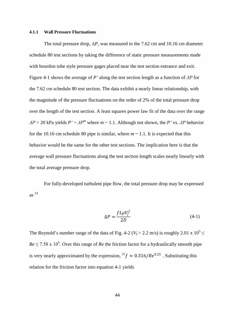
44
4.1.1 Wall Pressure Fluctuations
The total pressure drop, ΔP, was measured in the 7.62 cm and 10.16 cm diameter
schedule 80 test sections by taking the difference of static pressure measurements made
with bourdon tube style pressure gages placed near the test section entrance and exit.
Figure 4-1 shows the average of P’ along the test section length as a function of ΔP for
the 7.62 cm schedule 80 test section. The data exhibit a nearly linear relationship, with
the magnitude of the pressure fluctuations on the order of 2% of the total pressure drop
over the length of the test section. A least squares power law fit of the data over the range
ΔP > 20 kPa yields P’ ~ ΔPm where m ~ 1.1. Although not shown, the P’ vs. ΔP behavior
for the 10.16 cm schedule 80 pipe is similar, where m ~ 1.1. It is expected that this
behavior would be the same for the other test sections. The implication here is that the
average wall pressure fluctuations along the test section length scales nearly linearly with
the total average pressure drop.
For fully-developed turbulent pipe flow, the total pressure drop may be expressed
as 23
∆𝑃𝑃 =
𝑓𝑓𝐿𝐿𝜌𝜌𝑉𝑉𝑓𝑓2
2𝐷𝐷 (4-1)
The Reynold’s number range of the data of Fig. 4-2 (Vf > 2.2 m/s) is roughly 2.01 x 10⁵ ≤
Re ≤ 7.58 x 10⁵. Over this range of Re the friction factor for a hydraulically smooth pipe
is very nearly approximated by the expression, 21𝑓𝑓 ≈ 0.316/𝑅𝑅𝑒𝑒0.25 . Substituting this
relation for the friction factor into equation 4-1 yields

45
∆𝑃𝑃 ≈
0.158𝐿𝐿𝜌𝜌0.75𝑉𝑉𝑓𝑓1.75𝜇𝜇0.25
𝐷𝐷1.25 (4-2)
where μ is the absolute fluid viscosity. Based on the data shown in Fig. 4-1 and the
relationship shown in equation 4-2, it can be shown that P’ ~ ΔP ~ Vf2. This is what was
implied in section 2.3.
Shown in Fig. 4-2 is P’ as a functions of the average fluid speed (top panel) and
the average flow rate (bottom panel) in the pipes. Results are shown for all six test
sections listed in Table 3-1. The plots represent an average of the P’ measurements over
the six discrete axial locations along the pipe where pressure data were acquired. At low
speeds some scatter exists in the data due to resolution limits of the sensors. At higher
speeds however, (Vf > 2 m/s) the trend in the data is similar for all test sections. Namely,
Figure 4-1: P' as a function of the total pressure drop, ΔP, across the test section for the Schedule 80 7.62 cm test section.
0
500
1000
1500
2000
000.E+0 20.E+3 40.E+3 60.E+3 80.E+3
P' (P
a)
ΔP (Pa)

46
the P’ vs. Vf trend exhibits a power law relation, P’ ~ Vfm. A least squares fit to each data
set shown in Fig. 4-2 over the range Vf > 2.5 m/s reveals that m varies from 1.91 to 2.07
with an average value of 2.02. There appears to be no systematic variation in m, and the
difference between m and the expected value of 2.0 is less than 5%. Performing an
analysis of variance between the determined values of m and the expected value of 2.0
provides sufficient evidence to conclude that the variation in m is insignificant. This
result is in excellent agreement with the analysis of the P’ vs. ΔP data shown in Fig. 4-1
and Eqs. 4-1 and 4-2 and provides two independent measures showing that P’ scales
directly with the average fluid dynamic pressure (ρVf2).
When plotted as a function of Vf, the P’ data for the 10.16 cm diameter schedule
40 test section shows the largest magnitude at a given Vf. The magnitude of the P’ data
10.16 cm test sections appears to be larger than the data for the 7.62 cm test sections,
which are larger than the data for the 5.08 cm test sections. As expected, however, there
seems to be no systematic variation in P’ with diameter to thickness ratio (D/t). When
plotted as a function of Q (which is a function of D and Vf), the behavior of the
magnitude of P’ in the test sections appears to be reversed, with the data for the 5.08 cm
schedule 80 test section showing the largest P’ magnitude at a given Vf. Due to the large
uncertainty associated with the pressure measurements, comparison of the P’ magnitude
between test sections is somewhat suspect.

47
Figure 4-2: P' as a function of the average fluid speed, Vf (upper panel), and average flow rate, Q (lower panel), for flow through the six test sections.
100
1000
2 20
P'(P
a)
Vf (m/s)
D = 10.16 cm, Schedule 80D = 7.62 cm, Schedule 80D = 10.16 cm, Schedule 40D = 7.62 cm, Schedule 40D = 5.08 cm, Schedule 40D = 5.08 cm, Schedule 80
100
1000
0.007 0.07
P' (
Pa)
Q (m3/s)
D = 10.16 cm, Schedule 80D = 7.62 cm, Schedule 80D = 10.16 cm, Schedule 40D = 7.62 cm, Schedule 40D = 5.08 cm, Schedule 40D = 5.08 cm, Schedule 80
D = 10.16 cm, Schedule 80
D = 7.62 cm, Schedule 80
D = 10.16 cm, Schedule 40
D = 7.62 cm, Schedule 40
D = 5.08 cm, Schedule 40
D = 5.08 cm, Schedule 80
D = 10.16 cm, Schedule 80
D = 7.62 cm, Schedule 80
D = 10.16 cm, Schedule 40
D = 7.62 cm, Schedule 40
D = 5.08 cm, Schedule 40
D = 5.08 cm, Schedule 80

48
4.1.2 Accelerometer Measurements
4.1.2.1 A’ as a Function of P’
Figures 4-3 and 4-4 show A’ and V’ respectively as a function of P’ for each of
the six test sections. The trend in the data is similar to that shown in Fig. 4-2. For both A’
and V’ the data exhibit power law relations, Z’ ~ P’m, where Z’ represents A’ or V’. A
least squares fit of the data in Fig. 4-3 shows that m varies from 0.95 to 1.04 with an
average value of 1.01. The variation in m is again considered insignificant. This implies
that A’ scales as Vf2 as suggested in section 2.3.
Repeating a least squares fit for the data in Fig. 4-4 shows that m varies from 0.78
to 0.92 with an average value of 0.81. Raising P’ (i.e. Vf2) to this average power shows
Figure 4-3: A' as a function of P' for flow through the six test sections.
0.04
0.4
100 1000
A' (
m/s2 )
P' (Pa)
D = 10.16 cm, Schedule 80
D = 7.62 cm, Schedule 80
D = 10.16 cm, Schedule 40
D = 7.62 cm, Schedule 40
D = 5.08 cm, Schedule 40
D = 5.08 cm, Schedule 80
D = 10.16 cm, Schedule 80
D = 7.62 cm, Schedule 80
D = 10.16 cm, Schedule 40
D = 7.62 cm, Schedule 40
D = 5.08 cm, Schedule 40
D = 5.08 cm, Schedule 80
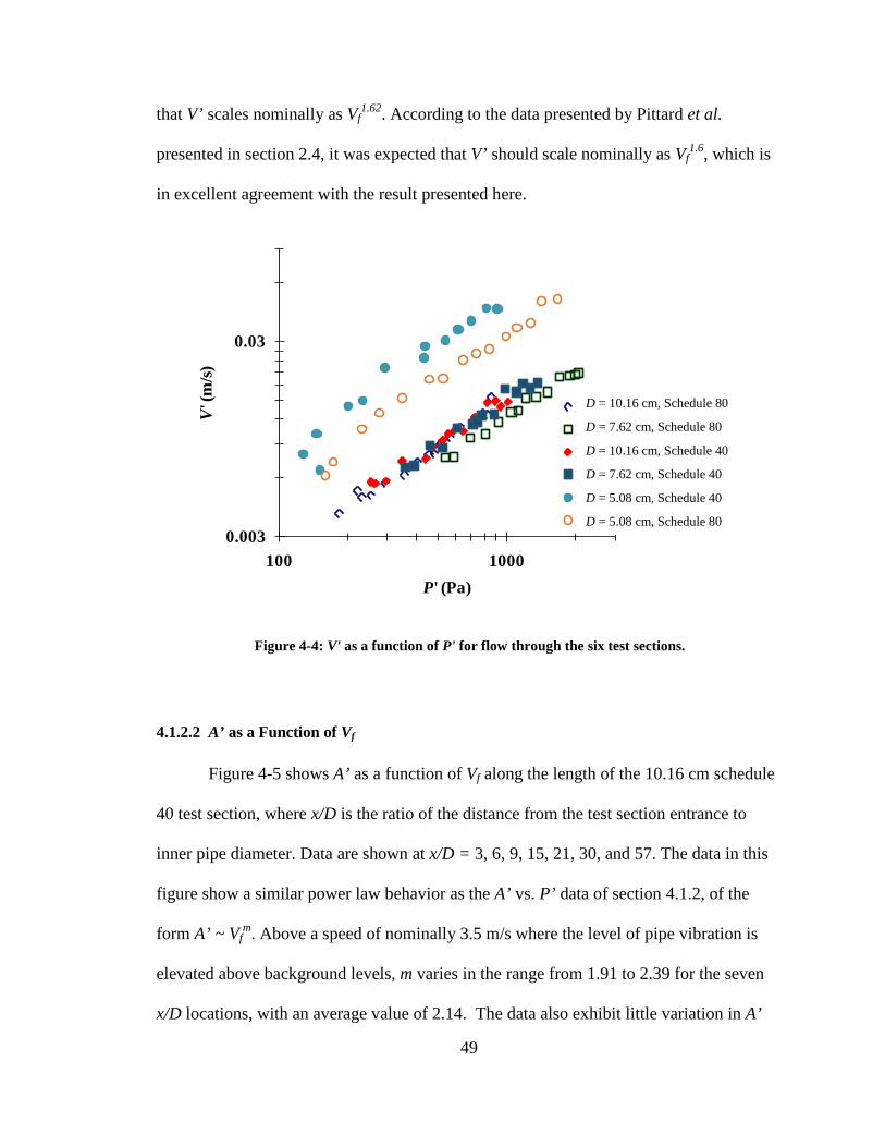
49
that V’ scales nominally as Vf1.62. According to the data presented by Pittard et al.
presented in section 2.4, it was expected that V’ should scale nominally as Vf1.6, which is
in excellent agreement with the result presented here.
4.1.2.2 A’ as a Function of Vf
Figure 4-5 shows A’ as a function of Vf along the length of the 10.16 cm schedule
40 test section, where x/D is the ratio of the distance from the test section entrance to
inner pipe diameter. Data are shown at x/D = 3, 6, 9, 15, 21, 30, and 57. The data in this
figure show a similar power law behavior as the A’ vs. P’ data of section 4.1.2, of the
form A’ ~ Vfm. Above a speed of nominally 3.5 m/s where the level of pipe vibration is
elevated above background levels, m varies in the range from 1.91 to 2.39 for the seven
x/D locations, with an average value of 2.14. The data also exhibit little variation in A’
Figure 4-4: V' as a function of P' for flow through the six test sections.
0.003
0.03
100 1000
V' (
m/s)
P' (Pa)
D = 10.16 cm, Schedule 80D = 7.62 cm, Schedule 80D = 10.16 cm, Schedule 40D = 7.62 cm, Schedule 40D = 5.08 cm, Schedule 40D = 5.08 cm, Schedule 80
D = 10.16 cm, Schedule 80
D = 7.62 cm, Schedule 80
D = 10.16 cm, Schedule 40
D = 7.62 cm, Schedule 40
D = 5.08 cm, Schedule 40
D = 5.08 cm, Schedule 80
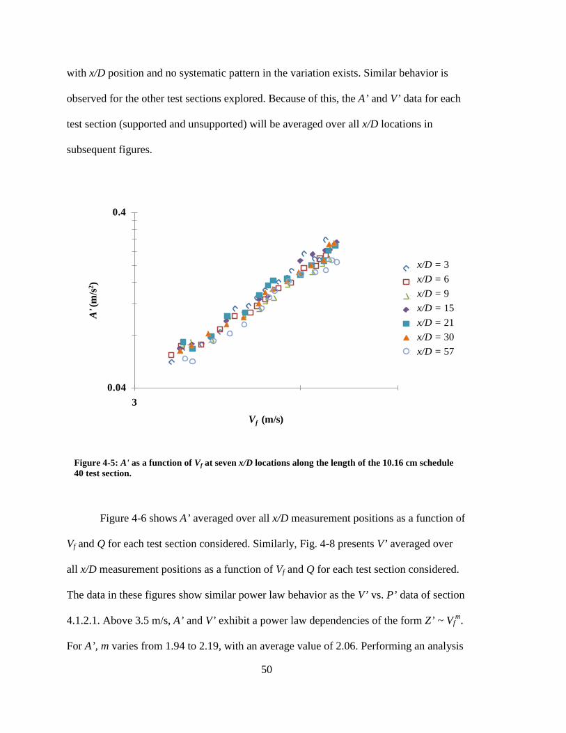
50
with x/D position and no systematic pattern in the variation exists. Similar behavior is
observed for the other test sections explored. Because of this, the A’ and V’ data for each
test section (supported and unsupported) will be averaged over all x/D locations in
subsequent figures.
Figure 4-6 shows A’ averaged over all x/D measurement positions as a function of
Vf and Q for each test section considered. Similarly, Fig. 4-8 presents V’ averaged over
all x/D measurement positions as a function of Vf and Q for each test section considered.
The data in these figures show similar power law behavior as the V’ vs. P’ data of section
4.1.2.1. Above 3.5 m/s, A’ and V’ exhibit a power law dependencies of the form Z’ ~ Vfm.
For A’, m varies from 1.94 to 2.19, with an average value of 2.06. Performing an analysis
Figure 4-5: A' as a function of Vf at seven x/D locations along the length of the 10.16 cm schedule 40 test section.
0.04
0.4
3
A' (
m/s2 )
Vf (m/s)
x/D = 3x/D = 6x/D = 9x/D = 15x/D = 21x/D = 30x/D = 57
x/D = 3 x/D = 6 x/D = 9 x/D = 15 x/D = 21 x/D = 30 x/D = 57

51
Figure 4-6: A' as a function of Vf (top panel) and Q (bottom panel) for flow through the six test sections considered.
0.04
0.4
3
A' (
m/s2 )
Vf (m/s)
D = 10.16 cm, Schedule 80D = 7.62 cm, Schedule 80D = 10.16 cm Schedule 40D = 7.62 cm, Schedule 40D = 5.08 cm, Schedule 40D = 5.08 cm, Schedule 80
0.03
0.3
0.006 0.06
A' (
m/s2 )
Q (m3/s)
D = 10.16 cm, Schedule 80D = 7.62 cm, Schedule 80D = 10.16 cm, Schedule 40D = 7.62 cm, Schedule 40D = 5.08 cm, Schedule 40D = 5.08 cm, Schedule 80
D = 10.16 cm, Schedule 80
D = 7.62 cm, Schedule 80
D = 10.16 cm, Schedule 40
D = 7.62 cm, Schedule 40
D = 5.08 cm, Schedule 40
D = 5.08 cm, Schedule 80
D = 10.16 cm, Schedule 80
D = 7.62 cm, Schedule 80
D = 10.16 cm, Schedule 40 D = 7.62 cm, Schedule 40 D = 5.08 cm, Schedule 40
D = 5.08 cm, Schedule 80

52
of variance on the values of m and the expected value of 2.0 indicates that the variation in
m is insignificant. When plotted as a function of Vf, the magnitude of A’ at a given Vf is
nominally 50% greater for the 10.16 cm and 5.08 cm test sections than for the 7.62 cm
test sections. Recall from section 2.4 that Evans et al., using a flow loop similar to the
one described in Chapter 3, obtained average values of the power law exponent m for A’
and V’ of 2.16 and 1.68 respectively. These values are only marginally greater than the
values of m for the current data, differing by about 8% and 5%, respectively.
Modest variation between schedule 40 and 80 data sets exist for each pipe
diameter, with the general trend being an increase in A’ with decreasing schedule size.
The wall thickness for all of the schedule 80 test sections is in the range 39-42% greater
than for the schedule 40 test sections, while the diameters differ in the range 3-6%
respectively. Surprisingly, the A’ vs. Vf data of Fig. 4-6 does not exhibit a systematic
variation with pipe diameter. The data for the intermediate diameter size (7.62 cm) lies
lower than for the other two diameter sizes.
When A’ is plotted as a function of Q, the behavior appears somewhat different,
although the values of the power law exponent m (A’ ~ Qm) remain the same. Here the
magnitude of A’ is systematic with pipe diameter where the 10.16 cm test section data
lies below the 7.62 cm test section which lies below the 5.08 cm test section data.
Figure 4-7 presents A’ as a function of the pipe diameter to thickness ratio, D/t,
for each test section and a constant fluid velocity of 6.7 m/s. Although there are only two
points for each pipe diameter, the trend illustrates that A’ increases with increasing D/t

53
although the dependency is not the same for varying pipe diameter. Similar conclusions
can be drawn from the data of Fig. 4-6 (top panel).
Figure 4-8 shows V’ as functions of Vf (top panel) and Q (bottom panel) for each
of the six test sections. The values of the power law exponent m (V’ ~ Vfm) range from
1.51 to 1.72, with an average value of 1.64. Again, the variation is deemed to be non-
systematic. This is also in good agreement with the expected scaling of Vf1.6, as stated in
section 4.1.2.1, based on the V’ vs. P’ data. Further, this is in good agreement with the
experimental results of Pittard et al.2 presented in section 2.4. When plotted as functions
of Vf (top panel) and Q (bottom panel), V’ behaves very similarly to the A’ data.
Specifically, the V’ vs. Vf data does not exhibit a systematic variation with pipe diameter.
However, when V’ is plotted as a function of Q the magnitude of V’ is systematic with
pipe diameter, where the 10.16 cm test section data lies below the 7.62 cm test section
data which lies below the 5.08 cm test section data. A notable difference is that
Figure 4-7: A' as a function of D/t at Vf ≈ 6.7 m/s for each the three diameter pipes considered.
0.05
0.1
0.15
0.2
0.25
0.3
8 10 12 14 16 18
A' (
m/s2 )
D/t
D = 5.08 cm
D = 7.62 cm
D = 10.16 cm
D = 5.08 cm D = 7.62 cm D = 10.16 cm

54
Figure 4-8: V' as a function of Vf (top panel) and Q (bottom panel) for flow through the six test sections considered.
0.003
0.03
3
V' (
m/s)
Vf (m/s)
D = 10.16 cm, Schedule 80D = 7.62 cm, Schedule 80D = 10.16 cm, Schedule 40D = 7.62 cm, Schedule 40D = 5.08 cm, Schedule 40D = 5.08 cm, Schedule 80
0.003
0.03
0.006 0.06
V' (
m/s)
Q (m3/s)
D = 10.16 cm, Schedule 80D = 7.62 cm, Schedule 80D = 10.16 cm, Schedule 40D = 7.62 cm, Schedule 40D = 5.08 cm, Schedule 40D = 5.08 cm, Schedule 80
D = 10.16 cm, Schedule 80
D = 7.62 cm, Schedule 80
D = 10.16 cm, Schedule 40
D = 7.62 cm, Schedule 40
D = 5.08 cm, Schedule 40
D = 5.08 cm, Schedule 80
D = 10.16 cm, Schedule 80
D = 7.62 cm, Schedule 80
D = 10.16 cm, Schedule 40
D = 7.62 cm, Schedule 40
D = 5.08 cm, Schedule 40
D = 5.08 cm, Schedule 80
55
there is more separation in the relative magnitudes of V’ between the 5.08 cm and 10.16
cm data sets, with the relative magnitude of the 5.08 cm data being noticeably larger than
the 10.16 cm data, when compared to A’ vs. Vf.
4.1.2.3 Acceleration Spectra
Power spectral densities (PSDs) were computed from the acceleration time series
data for each test section and at several velocities. Each PSD was then compared to the
frequency response of the corresponding test section which was excited with the impact
hammer described in section 3.3.
Frequency response data were collected by placing an accelerometer half way
down the length of a stationary water filled test section and striking the pipe several times
with the hammer adjacent to the accelerometer. Two seconds of data were collected per
impact at a rate of 5000 Hz. The pipe was struck five times and the resulting spectra were
averaged together. This average is referred to hereafter as the natural pipe response.
The PSDs were calculated for each data set by breaking the 10 seconds of
acceleration data into two second segments to keep the frequency resolution the same as
for the impact hammer data. These data segments were then normalized by dividing each
time segment by its standard deviation (A’) and are referred to as Anorm. The PSD was
then calculated by squaring the Fast Fourier Transform (FFT) of each Anorm and the five
PSDs were then averaged together. Finally, so that the integral of each averaged PSD
would equal one, it was divided by the square of its sample rate 23. This normalized PSD
is referred to as Ã.

56
Figures 4-9 and 4-10 show à for the 7.62 cm schedule 40 test section at average
flow speeds of 3.08, 4.96, (Fig. 4-9) 8.05, and 10.8 m/s (Fig. 4-10). Also included is the
natural pipe response and a line that indicates the -5/3 characteristic of turbulence decay.
At the lower velocities shown in it is possible to see peaks in à that correspond to peaks
in the natural pipe response. A notable feature of this plot is that although the à vs. f
distribution exhibits a modestly steeper decay than -5/3 at 3.08 and 4.96 m/s (f -2.24 at no
flow), this decay appears to approach f -5/3 as the flow speed increases. Also, between
400-500 Hz, a characteristic rise occurs at both flow speeds due to excitation of the
natural pipe response. Because of these corresponding rises, it appears that at these low
flow speeds the pipe response is sensitive to excitation in the pipe’s natural frequencies.
Figure 4-9: PSD for 7.62 cm schedule 40 test section with flow at speeds of 3.08 and 4.96 m/s. Also included is a line indicating a -5/3 relationship and the natural pipe response for reference.
Vf = 3.08 m/s
Vf = 4.96 m/s
Natural Pipe Response
f -5/3

57
At the higher flow speeds shown in Fig. 4-10, the spectra decay with a -5/3
relation and there is little to differentiate the Vf = 8.05 and Vf = 10.78 m/s spectra.
Specifically, there is no difference in the slope of the roll-off between the two spectra.
Also, the peaks in à at lower velocities associated with the natural pipe response are
significantly attenuated at the higher velocities, as is the low frequency content. The data
suggest that a greater fraction of the energy exists due to excitation at the natural pipe
response or low frequency pipe swaying. This increased low frequency energy content
appears to obscure the expected turbulent decay. However, at higher flow speeds, the
energy content shifts to a higher frequency range and the pipe vibrations detected by the
accelerometers appear to be due to the local turbulent fluctuations at the wall which
decay nominally as f -5/3.
Figure 4-10: PSD for 7.62 cm schedule 40 test section with flow at speeds of 8.05 and 10.78 m/s. Also included is a line indicating a -5/3 relationship and the natural pipe response for reference.
Vf = 8.05 m/s
Vf = 10.78 m/s
Natural Pipe Response
f -5/3

58
Figure 4-11 shows à for the 7.62 cm schedule 40 and 80 test sections at nearly the
same flow speed. Decreasing D/t from 14.22, for the 7.62 cm schedule 40 test section, to
9.67, for the 7.62 cm schedule 80 test section, does not appear to change the behavior of
the spectra. Similar to the data of Figs. 4-9 and 4-10, the decay begins at about 40 Hz and
exhibits a decay of nominally f -5/3.
Lastly, Fig. 4-12 illustrates the à behavior for the 5.08 cm, 7.62 cm, and 10.16 cm
schedule 40 test sections at a nominally constant flow speed of 6.7 m/s. Each à has been
multiplied by a base 10 factor (100 for the 5.08 cm test section, 0.1 for the 7.62 cm test
section, and 1x10⁻³ for the 10.16 cm test section) to separate the data sets. There is a spike
Figure 4-11: PSD for 7.62 cm schedule 40 and 80 test sections with average flow speeds of 10.78 m/s and 10.98 m/s, respectively. Also included is a line indicating a -5/3 relationship and the natural pipe response for reference.
Vf = 3.08 m/s
Vf = 3.08 m/s
f -5/3

59
in the à data at about 280 Hz for the 10.16 cm test section due to excitation in the natural
pipe response at the same frequency; however the à data from each test section decays
nominally as expected. Although not shown, similar to the à data presented in Fig. 4-9,
the decay of à is nominally steeper than f -5/3 at low flow speeds.
To summarize, it was shown in this section that for a pipe with no clamping
supports, P’ scales with A’, which in turn scales with the fluid dynamic pressure (~Vf2). It
was also shown that V’ scales with Vf1.6. Also, A’ was observed to increase with increased
D/t. Finally, Ã is influenced by to the natural pipe response at low flow speeds and was
Figure 4-12: PSD for the 5.08, 7.62, and 10.16 cm schedule 40 test sections at a flow speed of nominally 6.7 m/s. Each data set has been multiplied by 100 (5.08 cm test section), 0.1 (7.62 cm test section), and 1x10⁻³ (10.16 cm test section) to allow each data set to be delineated.
Vf = 6.7 m/s
Vf = 6.89 m/s
Vf = 6.77 m/s
f -5/3

60
observed to decay steeper than f -5/3. At high flow speeds, however, Ã is less sensitive to
the natural pipe response and the pipe vibrations appear to be due to local turbulent
fluctuations which decay nominally as f -5/3.
4.2 Pipe Wall Supports
4.2.1 Pipe Vibration vs. Support Length for the 10.16 cm Schedule 40 Pipe
Subsequent to the experiments in the unsupported test sections, experiments were
conducted employing the wall mounted clamp supports as described in section 3.6 to
investigate the influence of support length on A’. Figure 4-13 illustrates how A’ varies
with the six support separation lengths in the 10.16 cm schedule 40 test section. For the
experiments, accelerometers were placed exactly half way between the supports. Similar
to the no wall support cases, these data exhibit a power law dependency (A’ ~ Vfm) above
a flow speed of 3.5 m/s. The value of m here varies from 1.97 to 2.89 with an average
value of 2.34. For the no support and full support cases m is very near 2.0, while the half
and quarter support cases exhibit values of m ≈ 2.19 and 2.18, respectively. The shortest
support cases (eighth and sixteenth) however, have values of m approaching 3.0 (2.72 and
2.89, respectively) indicating that the magnitude of A’ exhibits a greater dependence on
Vf when the support length is very short. Although there is some variation in the value of
m with clamp support length, it can be seen that each data series is quite similar, with the
magnitude of A’ being the least for the full support case at high flow speeds.

61
Figure 4-14 illustrates how A’ varies with pipe clamp support length to pipe
diameter ratio (L/D) at four flow speeds (3.51 m/s, 4.26 m/s, 5.78 m/s and 6.73 m/s). At
flow speeds of 6.73 m/s and 5.78 m/s, it appears that the magnitude of A’ slightly
increases as L/D decreases (A’ ~ (L/D) -0.07), however at the lower flow speed of 3.51 m/s,
A’ appears to slightly decrease as L/D decreases (A’ ~ (L/D) 0.14) and is nominally flat at a
flow speed of 4.26 m/s. However, the A’ dependence on pipe clamp length appears to be
modest and not constant with L/D or average flow speed.
Figure 4-13: A' as a function of Vf for various wall support distances in the 10.16 schedule 40 test section.
0.03
0.3
3
A'(
m/s2 )
Vf (m/s)
No SupportFull Support1/2 Support1/4 Support1/8 Support1/16 Support

62
The influence of L/D on V’ is notably different than for the A’ data. Figure 4-15
gives V’ as a function of Vf for six pipe clamping length support scenarios and with the
10.16 cm schedule 40 test section. The values of m (V’ ~ Vfm) vary from 1.01 to 1.77 with
an average value, over the six clamping lengths, of 1.42. The average of m is about 1.65
for the longest wall support cases, but drops to an average of 1.11 for the eighth and
sixteenth support cases. This is in contrast to the A’ data where a modest increase with
decreasing support length was observed. Further, the data illustrate that the magnitude of
V’ decreases as the distance between the wall supports decreases. This is also apparent in
Fig. 4-16 which illustrates how V’ varies with L/D at four constant flow speeds. Also
evident in Fig. 4-16 is an increase in the magnitude of V’ with Vf and L/D.
Figure 4-14: A' as a function of L/D for four flow speeds in the 10.16 cm schedule 40 test section. The solid lines represent the trend in the data at Vf =6.73 and 3.51 m/s
0.04
0.4
2 20
A' (
m/s2 )
L/D
Vf = 6.73 m/sVf = 5.78 m/sVf = 4.26 m/sVf = 3.51 m/s
Vf = 6.73 m/s Vf = 5.78 m/s Vf = 4.26 m/s Vf = 3.51 m/s

63
The difference in the behavior of the A’ and V’ data is important. Although the A’
vs. Vf data are quite similar for all pipe clamp lengths, the V’ vs. Vf data show notable
differences. At shorter clamping length the pipe velocity is reduced whereas the pipe
acceleration remains nominally the same as for the long pipe. It should be noted,
however, that the wall supports are not perfect boundary conditions. Several meters of
pipe exist on either side of the supports which may mean that a stronger L/D relationship
may be confounded by bending and other vibrational pipe modes that may be transmitted
through the pipe due to the extra length of pipe on either side of the supports. The
clamping length cases that will be examined in more detail through the rest of this thesis
Figure 4-15: V' as a function of Vf for each pipe clamp length in the 10.16 cm schedule 40 test section. The solid lines illustrate how V' trends with Vf.
0.001
0.01
3
V' (
m/s)
Vf (m/s)
No SupportFull Support1/2 Support1/4 Support1/8 Support1/16 Support

64
are the no support case (freely hung), full wall support case, and quarter wall support
case.
4.2.2 Pipe Vibration for Varying Clamping Lengths and all Test Sections
The effect of clamp support length on A’ and V’ for each test section was also
investigated. As described in section 3.6, a 3.69 m subsection was defined in each test
section beginning 1.07 m from the test section entrance. This 3.69 m subsection is what is
considered a full support length. The downstream wall support was then moved to a
quarter of the full support length (quarter support). An accelerometer was then placed
Figure 4-16: V' as a function of L/D for four flow speeds in the 10.16 cm schedule 40 test section. The solid lines represent the trend in the data at Vf =6.73 and 3.51 m/s.
0.001
0.01
2 20
V' (
m/s)
L/D
Vf = 6.73 m/sVf = 5.78 m/sVf = 4.26 m/sVf = 3.51 m/s
Vf = 6.73 m/s Vf = 5.78 m/s Vf = 4.26 m/s Vf = 3.51 m/s

65
half way between the wall supports. For the no support case, the accelerometer remained
in the same position as for the full support case.
It is important to recall that for the 5.08 cm diameter test sections, developing
regions of both D = 5.08 cm and 10.16 cm were employed. This was done to explore
contraction effects when transitioning from a larger diameter pipe to a smaller diameter
pipe. Figure 4-17 presents A’ vs. Vf in the 5.08 cm test section. Two sets of data are
shown; one corresponding to the condition where the upstream pipe contracts from 10.16
cm and the other where no contraction exists. The data of Fig. 4-17 illustrate that the
contraction exerts negligible influence on the magnitude of A’ for the no wall support
case. The full wall support case exhibits similar behavior. For the quarter wall support
case, a modest increase in A’ is observed for the condition where the contraction exists.
The implication here is that using either developing region should not appreciably affect
the data. Generally, a contraction was avoided in all experiments, except for the baffle
plate experiments described in section 4.3 where the developing region was always D =
10.16 cm.

66
Conducting experiments on each test section with the three wall support
conditions described above (no support, full support, and quarter support) yield the
similar power law behavior described for the unsupported pipe. Table 4-1 lists the
average value of all six test section power law fit exponents (A’ and V’ ~ Vfm), m, under
the three clamping conditions. It also shows the standard deviation in m between each of
the six test sections. The standard deviations for the V’ data is the greatest, however
(except for the standard deviation in the values of m for the quarter support V’ data) the
values of m are within one standard deviation of the mean values presented in Table 4-1.
A 3% difference in the value m for the A’ data between the no clamp support case and the
full clamp support case exists and very little difference in the behavior of the two data
sets is observed when it is plotted. There is however, a modest increase of the value of m
for the quarter wall support case when compared to the no wall support case. This is
Figure 4-17: A’ as a function of Vf for the D = 5.08 cm schedule 80 test section with D = 5.08 cm and 10.16 cm developing regions and for the unsupported pipe case.
0.03
0.3
2.00 20.00
A'(m
/s2 )
Vf (m/s)
5.08 cm Developing Region
10.16 cm Developing Region

67
consistent with the behavior observed in section 4.2.1 for the 10.16 cm schedule 40 test
section.
The behavior observed in section 4.2.1 also appears to hold for V’ where m is
observed to decrease with decreasing L/D. The value of m for the no wall support case is
nominally 1.60 with a 14% and 17 % decrease in the value of m for the full and quarter
wall support cases, respectively.
Figure 4-18 compares the dependence of A’ on the ratio D/t for each test section
at the three clamp support lengths and a constant flow speed of 6.70 m/s. For all three
pipe diameters, the data exhibit an increase in the magnitude of A’ as D/t increases. The
A’ vs. D/t behavior is nominally the same for all three clamp lengths for the D = 7.62 cm
conditions with a smaller magnitude than the other pipe diameters. The greatest spread
exists for the D = 10.16 cm pipe diameter. Although the data presented in Fig. 4-18 is at
the same flow speed (6.7 m/s) the flow rates for these pipe diameters vary, with the
lowest flow in the 5.08 cm test sections and the highest in the 10.16 cm test sections. It
can be seen that the D/t dependence on A’ is not constant with fluid speed. It is also
apparent that D/t ratio on A’ is not constant with support length, suggesting differences in
Table 4-1: Average of each of the six test section power law exponents, m, (A’ and V’ ~ Vfm) for each
of the three clamping support lengths (no clamping, full clamping, and quarter clamping). Also displayed is the standard deviation of m over the six test sections.
m
A’ σ V’ σ No Wall Support 1.97 0.09 1.64 0.33
Full Wall Support 1.92 0.2 1.44 0.32
Quarter Wall Support 2.26 0.22 1.40 0.38

68
the pipe response are caused by the pipe clamp support length. This was also evident in
the data presented in Fig. 4-14.
To summarize, it was observed in the previous section that the dependence of A’
on D/t is not constant with flow rate, and that A’ is also influenced only weakly by L/D.
L/D does, however, have a greater influence on V’, where V’ generally increases as L/D
decreases. It was also observed that V’ has a decreasing dependence on Vf as the
clamping length decreases.
Figure 4-18: A’ vs. D/t at a flow speed of 6.70 m/s for each test section diameter (5.08 cm, 7.62 cm, and 10.16 cm) and the three clamping support lengths (no support, full support, quarter support).
0.05
0.1
0.15
0.2
0.25
0.3
8 10 12 14 16 18
A'(V
f) (m
/s2 )
D/t
D = 5.08 cm, No Sup
D = 7.62 cm, No Sup
D = 10.16 cm, No Sup
D = 5.08 cm, Full Sup
D = 7.62 cm, Full Sup
D = 10.16 cm, Full Sup
D = 5.08 cm, 1/4 Sup
D = 7.62 cm, 1/4 Sup
D = 10.16 cm, 1/4 Sup
D = 5.08 cm, No Support D = 7.62 cm, No Support D = 10.16 cm, No Support D = 5.08 cm, Full Support D = 7.62 cm, Full Support D = 10.16 cm, Full Support D = 5.08 cm, 1/4 Support D = 7.62 cm, 1/4 Support D = 10.16 cm, 1/4 Support

69
4.2.3 Accelerometer Spectra for Varying L/D
The accelerometer spectra for varying clamping lengths are now briefly explored.
Figure 4-19 shows a comparison of à for the unsupported and quarter supported 7.62 cm
schedule 40 test section. The flow speed for both support conditions is nominally 10.8
m/s. Ã has been multiplied by 1 x 10³ to separate the data sets on the figure for easier
comparison. The most apparent difference between the unsupported and quarter support
data is that the quarter support data exhibits a broad local rise in à from about 40-70 Hz.
This broad increase appears to be due to excitation in the natural pipe response in this
same frequency range. This behavior is observed in all flow speeds, but becomes more
distinguishable as flow speed increases. Above this frequency, the decay in à follows the
same pattern observed in the unsupported test section data. Namely, the decay is steeper
than an f -5/3 power law at low velocities, and approaches an f -5/3 decay as velocity
increases.
It is also apparent from the data of Fig. 4-19 that low frequency vibrations have
been significantly attenuated in the quarter wall support length. This short wall clamping
length appears to behave somewhat as a high pass filter. The data suggests that the pipe
response is more strongly influenced by the natural pipe response for the quarter support
case than for the unsupported case (Fig. 4-10). This likely occurs because the natural pipe
response for the quarter support case contains more energy at higher frequencies. This
sensitivity to the natural pipe response at short separation distances may hamper the
ability to infer turbulent flow behavior at the pipe wall.

70
Although not shown, the full support case exhibits similar behavior and sensitivity
to the natural pipe response as the unsupported case, suggesting that there is little
difference in the observed behavior of A’ between the unsupported case and the longest
wall support case (full wall support). This appears to signify that the distance between
wall supports affects the pipe wall acceleration more as the distance between the supports
becomes shorter.
Figure 4-19: Comparison of à vs. f for unsupported and quarter support 7.62 cm schedule 40 test sections with a flow speed of 10.78 m/s. The unsupported case has been multiplied by 1000 to make comparison easier.
Natural Pipe Response, 1/4 Support
Vf = 10.78 m/s, No Support
Vf = 10.78 m/s, 1/4 Support
f -5/3

71
4.3 Non-dimensionalization of A’
It has been previously shown that A’ scales nominally as Vf2 and D/t. In general,
the rms of the pipe wall acceleration can be written as a function of all the variables that
exert influence:
𝐴𝐴′ = 𝑓𝑓�𝑉𝑉𝑓𝑓 ,𝐷𝐷, 𝑡𝑡, 𝐿𝐿,𝜌𝜌, 𝜇𝜇,𝜌𝜌𝑒𝑒𝑒𝑒 ,𝜔𝜔𝑛𝑛 ,𝐸𝐸� (4-3)
where ωn is a natural frequency of each pipe section and contains dependence of the pipe
material modulus, E, and ρeq is the equivalent density of the water filled pipe, which is
defined as 24
𝜌𝜌𝑒𝑒𝑒𝑒 =
𝜌𝜌𝜌𝜌 �𝐷𝐷2�2
+ 𝜌𝜌𝑝𝑝2𝜌𝜌 �𝐷𝐷2 + 𝑡𝑡2� 𝑡𝑡
2𝜌𝜌𝑡𝑡 �𝐷𝐷2 + 𝑡𝑡2�
(4-4)
Recasting this set of dimensional variables into non-dimensional form following the
standard approach yields the following set of non-dimensional variables.
𝐴𝐴∗ =𝐴𝐴′𝑡𝑡𝑉𝑉𝑓𝑓2
(4-5)
𝑅𝑅𝑒𝑒 =𝜌𝜌𝑉𝑉𝑓𝑓𝐷𝐷𝜇𝜇
(4-6)
𝑡𝑡∗ =𝑡𝑡𝐷𝐷
(4-7)
𝐿𝐿∗ =𝐿𝐿𝐷𝐷
(4-8)
𝜌𝜌∗ =𝜌𝜌𝑒𝑒𝑒𝑒𝜌𝜌
(4-9)
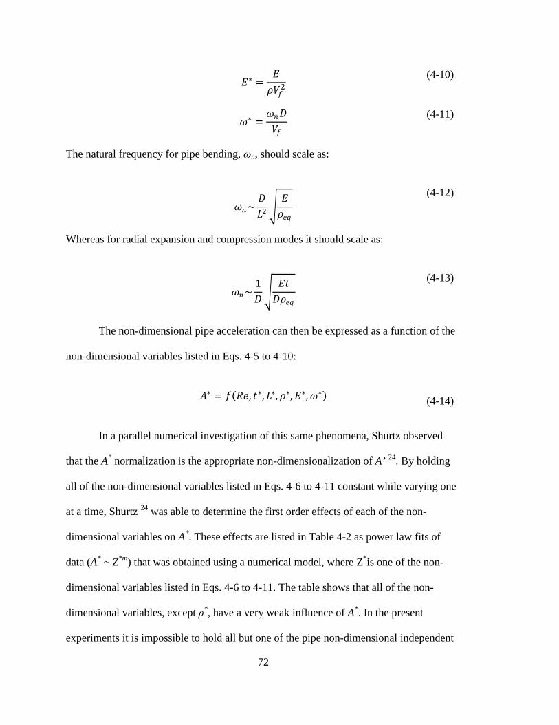
72
𝐸𝐸∗ =𝐸𝐸𝜌𝜌𝑉𝑉𝑓𝑓2
(4-10)
𝜔𝜔∗ =𝜔𝜔𝑛𝑛𝐷𝐷𝑉𝑉𝑓𝑓
(4-11)
The natural frequency for pipe bending, ωn, should scale as:
𝜔𝜔𝑛𝑛~
𝐷𝐷𝐿𝐿2 �
𝐸𝐸𝜌𝜌𝑒𝑒𝑒𝑒
(4-12)
Whereas for radial expansion and compression modes it should scale as:
𝜔𝜔𝑛𝑛~
1𝐷𝐷�
𝐸𝐸𝑡𝑡𝐷𝐷𝜌𝜌𝑒𝑒𝑒𝑒
(4-13)
The non-dimensional pipe acceleration can then be expressed as a function of the
non-dimensional variables listed in Eqs. 4-5 to 4-10:
𝐴𝐴∗ = 𝑓𝑓(𝑅𝑅𝑒𝑒, 𝑡𝑡∗, 𝐿𝐿∗,𝜌𝜌∗,𝐸𝐸∗,𝜔𝜔∗) (4-14)
In a parallel numerical investigation of this same phenomena, Shurtz observed
that the A* normalization is the appropriate non-dimensionalization of A’ 24. By holding
all of the non-dimensional variables listed in Eqs. 4-6 to 4-11 constant while varying one
at a time, Shurtz 24 was able to determine the first order effects of each of the non-
dimensional variables on A*. These effects are listed in Table 4-2 as power law fits of
data (A* ~ Z*m) that was obtained using a numerical model, where Z*is one of the non-
dimensional variables listed in Eqs. 4-6 to 4-11. The table shows that all of the non-
dimensional variables, except ρ*, have a very weak influence of A*. In the present
experiments it is impossible to hold all but one of the pipe non-dimensional independent

73
parameters constant. However, it is still useful to explore how A* depends on each
parameter.
Figure 4-20 illustrates A* as a function of Re for the six test sections examined, for
the unsupported scenario and for 2x10⁵ ≤ Re ≤ 8x10⁵. The magnitude of A* for the 10.16
cm test sections is greater than for the 7.62 cm and 5.08 cm test sections. It is also
apparent that the A* data for the 10.16 cm test sections collapse onto each other and
appear nominally flat. The A* data for each of the 7.62 cm and 5.08 cm test sections are
also observed to collapse onto each other, but appear to decrease slightly with increasing
Re. The values of m corresponding to A*~ Rem power law fits to the data show that the
dependence of A* on Re is nominally very weak (m ~ -0.018). The weak dependence of
A* on Re implies that A* is nominally constant with Re when the test section is
unclamped.
Table 4-2: The values of m corresponding to A*~ Z*m power law determined by a numerical simulation of flow induced pipe vibrations presented by Shurtz 24.
A*
Re -0.18
t* 0.04
L* -0.16
ρ* -1.00
E* 0.10
ω* -0.35

74
Figure 4-21 illustrates the same conditions as Fig. 4-20 for the full clamp support
case. The magnitude of the A* data for the 10.16 cm schedule 80 test section is greater
than for the 10.16 cm schedule 40 test section. The magnitude of A* for the 7.62 cm test
sections (which collapse onto each other) is also slightly greater than for the 5.08 cm test
sections (which also collapse onto each other). The values of m corresponding to A*~
Rem power law fits to the data show that the depedence of A* on Re is also nominally very
weak for the full clamp support (m ~ -0.021).
Figure 4-20: A* vs. Re for each of the six test sections considered and for no clamping support.
1.E-041.E+05 1.E+06
A*
Re
10.16 cm, Sch 407.62 cm, Sch 405.08 cm, Sch 4010.16 cm, Sch 807.62 cm, Sch 805.08 cm, Sch 80
D = 10.16 cm, Sch 40 D = 7.62 cm, Sch 40 D = 5.08 cm, Sch 40 D = 10.16 cm, Sch 80 D = 7.62 cm, Sch 80 D = 5.08 cm, Sch 80

75
Figure 4-22 illustrates the same conditions as Fig. 4-20 for the quarter clamp
support case. The magnitude of A* for the 10.16 cm test sections with the quarter
clamping length is greater than for the same test sections with longer clamping lengths.
Also, A* exhibits a slight increase in its dependence on Re for the 7.62 cm and 5.08 cm
test sections. The values of m corresponding to A*~ Rem power law fits to the data show
that the dependence of A* increases nominally at m ~ 0.22 with increasing Re and is listed
in Table 4-3.
Figure 4-21: A* vs. Re for each of the six test sections considered and for full clamping support.
1.E-041.E+05 1.E+06
A*
Re
10.16 cm, Sch 407.62 cm, Sch 405.08 cm, Sch 4010.16 cm, Sch 807.62 cm, Sch 805.08 cm, Sch 80
D = 10.16 cm, Sch 40
D = 7.62 cm, Sch 40
D = 5.08 cm, Sch 40
D = 10.16 cm, Sch 80
D = 7.62 cm, Sch 80
D = 5.08 cm, Sch 80

76
Table 4-3 lists the values of m corresponding to A*~ Rem power law fits to the data
for each of the six test sections considered and for the three clamp support lengths (no
support, full support, and quarter support). There appears to be no systematic pattern in
the variation of the values of m among the test sections. However, on average there is no
statistically significant difference in the values of m for the no support case and full
support case and the average values of m suggest no dependence of A* on Re. In contrast,
for the quarter clamping case a modest dependence on Re appears.
Figure 4-22: A* vs. Re for each of the six test sections considered and for the quarter clamping support.
8.E-05
8.E-04
1.E+05 1.E+06
A*
Re
10.16 cm, Sch 407.62 cm, Sch 405.08 cm, Sch 4010.16 cm, Sch 807.62 cm, Sch 805.08 cm, Sch 80
D = 10.16 cm, Sch 40 D = 7.62 cm, Sch 40 D = 5.08 cm, Sch 40 D = 10.16 cm, Sch 80 D = 7.62 cm, Sch 80 D = 5.08 cm, Sch 80

77
The dependence of A* on Re is slightly different than that observed in the
numerical simulations of Shurtz 24. This is likely due to the fact that Shurtz considered a
hydraulically smooth pipe and the results of the experiments show that the pipes
employed exhibit behavior characteristic of rough pipes where the influence of Re is less
pronounced.
The dependence of A* on E*, ω*bend, and ω*
radial is nearly identical to that
described above for Re. Namely, for the unsupported and full support scenarios no
statistically significant variation of A* with each of the parameters exists. However, for
the quarter support case a modest dependence exists in the data. In fact, for ω*bend and
ω*radial, the power-law fit exponents are very similar to those listed in Table 4-3 for Re.
For E* the power law fit exponents are very nearly one half of those listed in Table 4-3
for Re.
Table 4-3: The values of m corresponding to A*~ Rem power law for each of the six test sections considered and the three clamping support lengths.
m Clamping Support Condition
No Full Quarter
10.16 cm, Sch 40 0.012 0.157 0.12
10.16 cm, Sch 80 0.137 -0.11 0.053
7.62 cm, Sch 40 -0.09 0.012 0.189
7.62 cm, Sch 80 0.015 -0.08 0.204
5.08 cm, Sch 40 -0.11 0.094 0.41
5.08 cm, Sch 80 -0.07 -0.2 0.322
Average -0.018 -0.021 0.22

78
Figure 4-23 illustrates A* as a function of t* for each of the three unsupported test
section diameters. The values of A* for each respective test section have been averaged
over a range of Re where negligible variation exists (2x10⁵ ≤ Re ≤ 8x10⁵). As with the A*
vs. Re data, the magnitude of A* for the 10.16 cm test sections is greater than for the 5.08
cm test sections, which is also greater than for the 7.62 cm test sections. Also, A* appears
nominally flat for the 10.16 cm and 5.08 cm test sections and modestly increases its
dependence on t* for the 7.62 cm test sections. The values of m corresponding to A*~ t*m
power law fits of the data show that the dependence of A* on t* is very weak (m ~ 0.08).
This value is twice the value predicted by Shurtz 24, listed in Table 4-2.
Figure 4-23: A* vs. t* for the three pipe diameters for the unsupported pipe. The values of A* have been averaged over a range of Re where there was little variation in A*.
1.E-040.05
A*
t*
10.16 cm test sections
7.62 cm test sections
5.08 cm test sections
D = 10.16 cm test sections
D = 7.62 cm test sections
D = 5.08 cm test sections

79
Figure 4-24 now illustrates A* as a function of ρ* for each of the three unsupported
test section diameters. Like in Fig. 4-23, the values of A* for each respective test section
have been averaged over the same Re range as listed for Fig. 4-23. The data shown in this
figure also show the same pattern in the relative magnitudes of A* as was shown in Fig. 4-
23. Specifically, the magnitude of A* is greatest for the 10.16 cm test sections followed
by the 5.08 cm test sections and then by the 7.62 cm test sections. The values of m
corresponding to A*~ ρ*m power law fits of the data show that the dependence of A*
decreases as ρ* increases (nominally m ~ -0.22). Shurtz predicts a value of m of -1.0 24.
Shurtz obtained this value by using a wider range in ρ* and by changing ρ* while keeping
D and t the same 24, which was not possible to do for this research.
Figure 4-24: A* vs. ρ* for the three pipe diameters for the unsupported pipe. The values of A* have been averaged over a range of Re where there was little variation in A*.
1.E-043.00
A*
ρ*
10.16 cm test sections
7.62 cm test sections
5.08 cm test sections
D = 10.16 cm test sections
D = 7.62 cm test sections
D = 5.08 cm test sections
80
The results of the numerical investigation of Shurtz suggests that to a first order
the pipe wall vibrations should scale as A’~ Vf2/t*ρ* for an unsupported pipe 24. Figures 4-
25 and 4-26 illustrate A’ as a function of only Vf2/t and then of Vf
2/t*ρ*, respectively.
Figure 4-25 shows A’ as a function of Vf2/t for each of the six unsupported test
sections considered. This figure also includes linear fits to the data with a zero intercept
that pass through the schedule 40 and 80 test section data for each pipe diameter (10.16
cm, 7.62 cm, and 5.08 cm). This functional relationship causes A’ for the schedule 40 and
80 data from each diameter test section to collapse onto each other. This relationship does
not, however, collapse the three pipe diameters onto each other. The magnitude of the
collapsed 10.16 cm data is nominally twice the magnitude of the collapsed 5.08 cm data
at a given Vf2/t. Also, the magnitude of the collapsed 7.62 cm data is nominally 20%
greater than the collapsed 5.08 cm data at a given Vf2/t. The average of the values of m
corresponding to A’~ (Vf2/t)m power law fits for each of the six test sections is very nearly
linear (m ~ 0.99), justifying the linear fit curves. Because this functional relationship does
not collapse the A’ data for the three pipe diameters onto each other, there is some other
parameter that influences the behavior of A’ that has not yet been captured. It is expected
that the A’~ Vf2/t*ρ* relationship will capture more of that behavior and cause a better
collapse of the data.

81
Shown in Fig. 4-26 is A’ as a function of Vf2/t*ρ* for each of the six unsupported
test sections considered. This figure also includes linear fit curves with a zero intercept
that pass through the schedule 40 and 80 test section data for each pipe diameter (10.16
cm, 7.62 cm, and 5.08 cm). This functional relationship does not cause as tight of a
collapse of the schedule 40 and 80 data from the 10.16 cm and 5.08 cm diameter test
sections as shown in Fig. 4-25. It does, however, cause the data from the 10.16 cm and
5.08 cm test sections to collapse onto each other. The 7.62 cm schedule 40 and 80 data
also collapse onto each other, however, the magnitude of this collapsed data is nominally
half of the 10.16 cm and 5.08 cm collapsed data. As illustrated by the linear fit lines, the
10.16 cm and 5.08 cm data collapse shown in Fig. 4-26 is tighter than the collapse of the
Figure 4-25: A’ vs. Vf2/t for each of the six unsupported test sections considered. Linear fit lines
with zero intercept pass through the schedule 40 and 80 pipe section data for each diameter.
0.04
0.40
1.E+03 1.E+04 1.E+05
A'
Vf2/t
10.16 cm, Sch 407.62 cm, Sch 405.08 cm, Sch 4010.16 cm, Sch 807.62 cm, Sch 805.08 cm, Sch 80Linear (10.16)Linear (7.62)Linear (5.08)
10.16 cm fit7.62 cm fit5.08 cm fit
D = 10.16 cm, Sch 40
D = 7.62 cm, Sch 40
D = 5.08 cm, Sch 40
D = 10.16 cm, Sch 80
D = 7.62 cm, Sch 80
D = 5.08 cm, Sch 80
D = 10.16 cm fit
D = 7.62 cm fit
D = 5.08 cm fit

82
7.62 cm and 5.08 cm data shown in Fig. 4-25. This appears to imply that the parameter
Vf2/t*ρ* captures more of the behavior of A’ than the parameter Vf
2/t.
Figure 4-27 shows A’ as a function of Vf2/t*ρ* for the data presented by Pittard et
al. 2. This functional relationship causes A’ for each pipe material and diameter (except
for the 3.81 cm stainless steel test section) to collapse onto one another. What is
interesting to note is that although these data were collected from a different facility and
the pipe moduli and densities vary greatly, the functional relationship, A’~ Vf2/t*ρ*, works
very well to collapse most of the data.
Figure 4-26: A’ vs. Vf2/ρ*t* for each of the six unsupported test sections considered. Linear fit
lines with zero intercept pass through the schedule 40 and 80 pipe section data for each diameter test section.
0.04
0.40
30 300
A'
Vf2/ρ*t*
10.16 cm, Sch 407.62 cm, Sch 405.08 cm, Sch 4010.16 cm, Sch 807.62 cm, Sch 805.08 cm, Sch 80Linear (10.16)Linear (7.62 cm)Linear (5.08 cm)7.62 cm fit5.08 cm fit
10.16 cm fit
D = 10.16 cm, Sch 40
D = 7.62 cm, Sch 40
D = 5.08 cm, Sch 40
D = 10.16 cm, Sch 80
D = 7.62 cm, Sch 80
D = 5.08 cm, Sch 80
D = 10.16 cm fit
D = 7.62 cm fit
D = 5.08 cm fit

83
Lastly, Figure 4-28 illustrates A’ as a function of the correlation Vf2.12βD1.9 for
each of the six unsupported test sections considered, where β is defined in Eq. 2-7. Figure
4-29 shows the same correlation applied to the data presented by Pittard et al. 2. This
correlation was developed previously by performing a statistical analysis on the 10.16 cm
and 7.62 cm schedule 40 and 80 data and is included here for completeness. Similar to
Fig. 4-25, the correlation used for Fig. 4-28 cause some of the data to collapse. The
difference is that in Fig. 4-28 the A’ data for the 10.16 cm and 7.62 cm test sections
collapse onto one another; whereas in Fig. 4-25, the A’ data for the 5.08 cm and 7.62 cm
test sections collapse onto one another. Also, in Fig. 4-28, the collapsed A’ data for the
5.08 cm test sections is nominally three times greater than the collapsed 10.16 cm and
Figure 4-27: A’ vs. Vf2/ρ*t* for the data presented by Pittard et al. 2.
0.0001
0.001
0.01
0.1
1 10 100 1000
A'
Vf2/ρ*t*
D = 7.62 cm PVC
D = 10.16 cm PVC
D = 7.62 cm AluminumD = 7.62 cm Stainless SteelD = 3.81 cm Stainless Steel
D = 7.62 cm PVC
D = 10.16 cm PVC
D = 7.62 cm Aluminum D = 7.62 cm Stainless Steel D = 3.81 cm Stainless Steel

84
7.62 cm data. When this correlation is applied to the data of Pittard et al.2 shown in Fig.
4-29, it causes the data from each pipe material to collapse fairly well. Although the 7.62
cm stainless steel data follows the same trend, its magnitude is slightly less than the rest
of the collapsed data. The notable exception to the data collapse is the magnitude of the
A’ data from the 3.81 cm stainless steel test section, which is nominally three times less
than the rest of the collapsed data. This correlation was developed previous to the
acquisition of the data for the 5.08 cm test sections and while it yielded a good collapse
of the original data, it is clear that it is not suitable for a large range of pipe diameters.
Figure 4-28: A’ vs. Vf2.12βD1.9 for each of the six unsupported test sections considered.
0.02
0.2
0.030 0.300
A'(m
/s2 )
Vf2.12βD1.9
10.16 cm, Sch 407.62 cm, Sch 405.08 cm, Sch 4010.16 cm, Sch 807.62 cm, Sch 805.08 cm, Sch 80
D = 10.16 cm, Sch 40
D = 7.62 cm, Sch 40
D = 5.08 cm, Sch 40
D = 10.16 cm, Sch 80
D = 7.62 cm, Sch 80
D = 5.08 cm, Sch 80
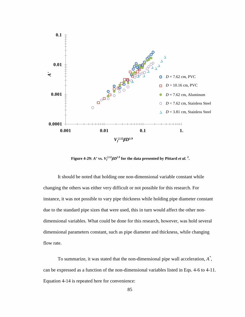
85
It should be noted that holding one non-dimensional variable constant while
changing the others was either very difficult or not possible for this research. For
instance, it was not possible to vary pipe thickness while holding pipe diameter constant
due to the standard pipe sizes that were used, this in turn would affect the other non-
dimensional variables. What could be done for this research, however, was hold several
dimensional parameters constant, such as pipe diameter and thickness, while changing
flow rate.
To summarize, it was stated that the non-dimensional pipe wall acceleration, A*,
can be expressed as a function of the non-dimensional variables listed in Eqs. 4-6 to 4-11.
Equation 4-14 is repeated here for convenience:
Figure 4-29: A’ vs. Vf2.12βD1.9 for the data presented by Pittard et al. 2.
0.0001
0.001
0.01
0.1
0.001 0.01 0.1 1.
A'
Vf2.12βD1.9
D = 7.62 cm PVC
D = 10.16 cm PVC
D = 7.62 cm Aluminum
D = 7.62 cm Stainless SteelD = 3.81 cm Stainless Steel
D = 7.62 cm, PVC
D = 10.16 cm, PVC
D = 7.62 cm, Aluminum
D = 7.62 cm, Stainless Steel
D = 3.81 cm, Stainless Steel

86
𝐴𝐴∗ = 𝑓𝑓(𝑅𝑅𝑒𝑒, 𝑡𝑡∗, 𝐿𝐿∗,𝜌𝜌∗,𝐸𝐸∗,𝜔𝜔∗)
Re-dimensionalizing A* gives:
𝐴𝐴′ =
𝑉𝑉𝑓𝑓2
𝑡𝑡𝑓𝑓(𝑅𝑅𝑒𝑒, 𝑡𝑡∗, 𝐿𝐿∗,𝜌𝜌∗,𝐸𝐸∗,𝜔𝜔∗) (4-15)
It was found that the non-dimensionalized pipe wall vibration, A*, was a very
weak function of Re, t*, E*, and ω*, showing good agreement with the numerical results
of Shurtz 24. Although experimental results varied greatly from the numerical results, it
was found that A* had the strongest functional dependence on ρ*. The variation between
the numerical and experimental results was most likely due to the ability to numerically
change one non-dimensional parameter without changing the others, thereby eliminating
confounding results. The functional relationship of these non-dimensional parameters
was weakest for the longest clamping support cases and became slightly more important
as the clamping length became short. To a first order, the scaling A’~ Vf2/t*ρ* provides a
good estimate of the rms of the pipe wall acceleration for long or unsupported pipe
sections.
4.4 Baffle Plate Influence
4.4.1 Various Baffle Plate Sizes
As discussed in section 3.2 baffle plates were inserted at the test section entrance
as turbulence inducers. Five plates were used, each with a different diameter and number
of holes drilled into them. The diameters of the holes were 2.54 cm, 1.27 cm, 0.635 cm,
0.318 cm, and 0.159 cm, with the hole diameter being how each baffle plate is

87
distinguished in this thesis. The plates were fabricated so that the through area of the
holes was 35.48 cm2, resulting in various numbers of holes in each plate (e.g. seven holes
for the 2.54 cm plate, 28 holes for the 1.27 cm baffle plate, 112 holes for the 0.635 cm
baffle plate, 448 holes for the 0.318 cm baffle plate, and 1793 holes for the 0.159 cm
plate). The 10.16 cm schedule 40 test section was the only test section used for the baffle
plate experiments.
Figure 4-30 illustrates the effects on A’ due to each baffle plate at various flow
velocities and at a streamwise distance of 0.305 m from the baffle plate. The data is
plotted versus the ratio of the baffle plate thickness to hole diameter. The data from each
baffle plate is contained in the vertical columns of data, with the largest baffle plate on
the left (tbaffle/Dhole = 0.25).
It can be seen in Fig. 4-30 that the 2.54 cm and 1.27 cm baffle plates (tbaffle/Dhole =
0.25 and 0.5 respectively) result in the largest increases in the magnitude of A’; although
for all baffle plates the pipe acceleration increases. The largest increases are caused by
cavitation that occurs in the largest baffle plates which was accompanied by audible
noise. Evidence of cavitation can be seen to occur in Fig. 4-29 between a flow speed of
3.07 m/s and 3.72 m/s with the 2.54 cm baffle plate. At this Vf the magnitude of A’
suddenly jumps. Although not as apparent, cavitation appears to occur between 3.07 m/s
and 3.97 m/s in the 1.27 cm baffle plate. What is also evident is that as tbaffle/Dhole
increases, the magnitude of A’ decreases; apparently due to an upward shift in the
velocity at which cavitation occurs and a reduction in the size of turbulent eddies formed.
This shift can be seen as the baffle plate hole size decreases, with cavitation setting up

88
only at the highest velocities in the 0.635 cm baffle plate and not at all in the smallest
baffle plates.
Recall that Fig. 4-5 presents A’ as a function of Vf for seven locations along the
length of the test section (x/D). For the no baffle plate scenario previously noted, in
section 4.1.2.2, there is no systematic variation in A’ with varying x/D. Figure 4-31 shows
significantly different behavior for the 2.54 cm baffle plate scenario. The figure shows A’
as a function of Vf at various x/D locations along the test section. Also shown are data for
the no baffle plate scenario. As previously stated, cavitation is occurring at the baffle
plate holes, for this plate, and its effect on A’ propagates down the entire length of the test
section. Cavitation appears to be initiated at a fluid speed of about 3 m/s causing A’ to
Figure 4-30: A' as a function of tbaffle/Dhole for various flow velocities in the 10.16 cm schedule 40 test section and each of the five baffle plates.
0.01
0.1
1
10
0.1 1 10
A'(
m/s2 )
tbaffle/Dhole
Vf = 5.83 m/sVf = 5.03 m/sVf = 4.37 m/sVf = 3.97 m/sVf = 3.72 m/sVf = 3.07 m/sVf = 2.43 m/s
Vf = 5.83 m/s Vf = 5.03 m/s Vf = 4.37 m/s Vf = 3.97 m/s Vf = 3.72 m/s Vf = 3.07 m/s Vf = 2.43 m/s

89
rise rapidly with increasing Vf. At a flow speed of nominally 4 m/s, the rate of increase in
A’ levels off and becomes similar at all x/D. The magnitude of A’ decreases with
increasing x/D and decreases towards the vibration levels of the no baffle plate scenario
at large x/D. A power law curve fit (A’ ~ Vfm) to the data above a flow speed of 4 m/s
results in values of the power, m, ranging from 4.12 to 3.36 for the various x/D positions
and is included in Table 4-4. At x/D = 3 and a flow speed of nominally 5.5 m/s, A’ is
observed to be about 300 times greater than for the no baffle plate case and at x/D = 57
(end of the test section), A’ is nominally 20 times greater.
Figure 4-31: A' vs. Vf at seven x/D locations along the test section length with the 2.54 cm baffle plate. A' for the test section with no baffle plate has been included for reference.
0.01
0.1
1
10
1 10
A' (
m/s2 )
Vf (m/s)
x/D = 3x/D = 6x/D = 9x/D = 15x/D = 21x/D = 30x/D = 57Average, No Baffle Plate
x/D = 3 x/D = 6 x/D = 9 x/D = 15 x/D = 21 x/D = 30 x/D = 57 Average, No Baffle Plate

90
Figures 4-32 and 4-33 show A’ as a function of Vf for the 0.635 cm baffle plate
(tbaffle/Dhole=1.0) and 0.159 cm baffle plate (tbaffle/Dhole=4.0), respectively. In Fig. 4-32,
cavitation appears to be initiating only at the highest flow speed. Further, the magnitude
of A’ is significantly lower than what was shown for the 2.54 cm baffle plate data in Fig.
4-33. At a flow speed of nominally 5.5 m/s, A’ is only about 10 times greater than for the
no baffle plate case at x/D = 3. A power law fit of the data with the exponents included in
Table 4-4, shows that as x/D increases the value of m approaches the no baffle plate case.
This becomes even more apparent for the 0.159 cm baffle plate (Fig. 4-32). Here the
magnitude of A’ at x/D = 3 is only about two times greater than for the no baffle plate
case. The value of m also changes very little with x/D, with an average value of 2.04.
These values are also included in Table 4-4. There appears to be little systematic
variation in the value of m with x/D for the 0.159 cm baffle plate scenario. However, for
the 0.635 cm baffle plate scenario, the value of m decreases with increasing x/D. The
values of m appear exhibit the same behavior for the 2.54 cm baffle plate except at the
end of the test section, where the values of m begin to increase again. Comparing the
values of m for the three baffle plate scenarios presented in Table 4-4 the general trend is
that m increases with increasing baffle plate hole diameter.

91
Figure 4-32: A' vs. Vf at seven x/D locations along the test section length with the 0.635 cm baffle plate. A' for the test section with no baffle plate has been included for reference.
Figure 4-33: A' vs. Vf at seven x/D locations along the test section length with the 0.159 cm baffle plate. A' for the test section with no baffle plate has been included for comparison.
0.01
0.1
1
10
1 10
A' (
m/s2 )
Vf (m/s)
x/D = 3x/D = 6x/D = 9x/D = 15x/D = 21x/D = 30x/D = 57Average, No Baffle Plate
0.01
0.1
1
1 10
A' (
m/s2 )
Vf (m/s)
x/D = 3x/D = 6x/D = 9x/D = 15x/D = 21x/D = 30x/D = 57Average, No Baffle Plate
x/D = 3 x/D = 6 x/D = 9 x/D = 15 x/D = 21 x/D = 30 x/D = 57 Average, No Baffle Plate
x/D = 3 x/D = 6 x/D = 9 x/D = 15 x/D = 21 x/D = 30 x/D = 57 Average, No Baffle Plate

92
Figure 4-34 shows A’ as a function of Vf for all five baffle plates at x/D = 3. As
expected, A’ is greatest for the largest diameter baffle plate holes at all Vf. When
cavitation is not occurring and as the baffle plate hole size decreases, the dependence of
A’ on Vf appears to approach the no baffle plate scenario. The primary difference is that
there is an upward offset in the magnitude of A’ that corresponds to the size of the baffle
plate holes. Cavitation exists for the 2.54 cm baffle plate above about 3 m/s and it exists
for the 1.27 cm baffle plate above a speed of nominally 3.5 m/s. For the 0.635 cm baffle
plate, cavitation appears to exist above 6.7 m/s.
Table 4-4: The value of m from a power law fit of the 2.54 cm, 0.635 cm, and 0.159 cm baffle plate data with x/D.
Baffle Plate Hole Size x/D 2.54 cm 0.635 cm 0.159 cm No Plate 3 4.12 2.93 2.02
2.03
6 3.78 2.75 1.92 9 3.54 2.45 2.29 15 3.36 2.28 2.19 21 3.70 2.03 1.89 30 3.47 1.95 2.00 57 3.85 2.09 1.98
Average 3.69 2.35 2.04

93
Figure 4-35 presents A’ as a function of Vf at x/D = 30. At this streamwise
position, the magnitude of A’ has dropped nominally by a factor of 10 for all baffle
plates. For the scenarios where cavitation does not exist, the magnitude of A’ is
approaching the no baffle plate case results. This indicates that A’ decays with increasing
distance from the baffle plate. Recall from equation 3-1 and section 3.1 that for turbulent
pipe flow to be considered fully developed Le/D ~ 44 (𝐿𝐿𝑒𝑒𝐷𝐷≈ 4.4𝑅𝑅𝑒𝑒
16). At x/D = 30, this
streamwise position is nearly far enough away from the baffle plates for the flow to be
considered fully developed again. The implication is that sufficiently far away from a
Figure 4-34: A’ vs. Vf at x/D = 3 for all five baffle plates. A’ for the no baffle plate case is included for comparison.
0.01
0.1
1
10
1 10
A' (
m/s2 )
Vf (m/s)
2.54 cm baffle plate1.27 cm baffle plate0.635 cm baffle plate0.318 cm baffle plate0.159 cm baffle plateNo Baffle Plate

94
turbulence source that is not inducing cavitation, the magnitude of A’ approaches a
condition representative of the baseline fully-developed turbulent pipe flow.
Figure 4-36 illustrates how the magnitude of A’ decays with x/D for each baffle
plate case at a constant flow speed of 3.61 m/s. As expected, the magnitude of A’ for the
no baffle plate case is nominally flat along the test section length. Although the flow
velocity is relatively low, cavitation is occurring with the 2.54 cm and 1.27 cm baffle
plates. For these cases, the decay in the magnitude of A’ appears to be steeper than for the
three other scenarios. The test section may not be long enough for A’ to return to the
baseline levels characteristic of the no baffle plate case. The magnitude of A’ for the
Figure 4-35: A’ vs. Vf at x/D = 30 for all five baffle plates. A' for the no baffle plate case is included for comparison.
0.01
0.1
1
10
1 10
A' (
m/s2 )
Vf (m/s)
2.54 cm baffle plate1.27 cm baffle plate0.635 cm baffle plate0.318 cm baffle plate0.159 cm baffle plateNo Baffle Plate baffle plate
2.54 cm Baffle Plate 1.27 cm Baffle Plate 0.635 cm Baffle Plate 0.318 cm Baffle Plate 0.159 cm Baffle Plate No Baffle Plate

95
0.318 cm and 0.159 cm baffle plates has decayed to the no baffle plate values by
nominally x/D = 9. For the 0.635 cm baffle plate A’ decays to the baseline value at x/D =
15.
As the flow speed increases to 6.84 m/s, as illustrated by the results of Figure 4-
36, it is evident that the decay in the magnitude of A’ is pushed further downstream. In
the cases where cavitation is occurring, the magnitude of A’ doesn’t begin to level off
until above x/D = 30. The magnitude of A’ with the 0.318 cm and 0.159 cm baffle plate
has decayed to the no baffle plate levels by x/D = 15, and by x/D = 30 for the 0.635 cm
baffle plate.
Figure 4-36: The decay of A' with x/D for each baffle plate case at a flow speed of 3.61 m/s.
0.01
0.1
1
1 10 100
A' (
m/s2 )
x/D
2.54 cm baffle plate1.27 cm baffle plate0.635 cm baffle plate0.318 cm baffle plate0.159 cm baffle plateNo Baffle Plate

96
To summarize, cavitation was observed occur with the 2.54 cm and 1.27 cm
baffle plates at flow speeds as low as nominally 3 m/s. Upon initiation of cavitation, the
magnitude of A’ near the baffle plate increased by up to 300 times of the baseline no
baffle plate case. As the distance from the baffle plates increased, the level of A’ for each
baffle plate case decreases toward the baseline. It was observed that the flow speed at
which cavitation is initiated increases as the baffle plate hole size decreases. Also, with
the baffle plates where cavitation does not occur, A’ decays to the baseline at an x/D
location that increases with Vf.
Figure 4-37: The decay of A' with x/D for each baffle plate case at a flow speed of 6.84 m/s.
0.1
1
10
100
1 10 100
A' (
m/s2 )
x/D
2.54 cm baffle plate1.27 cm baffle plate0.635 cm baffle plate0.318 cm baffle plate0.159 cm baffle plateNo Baffle Plate
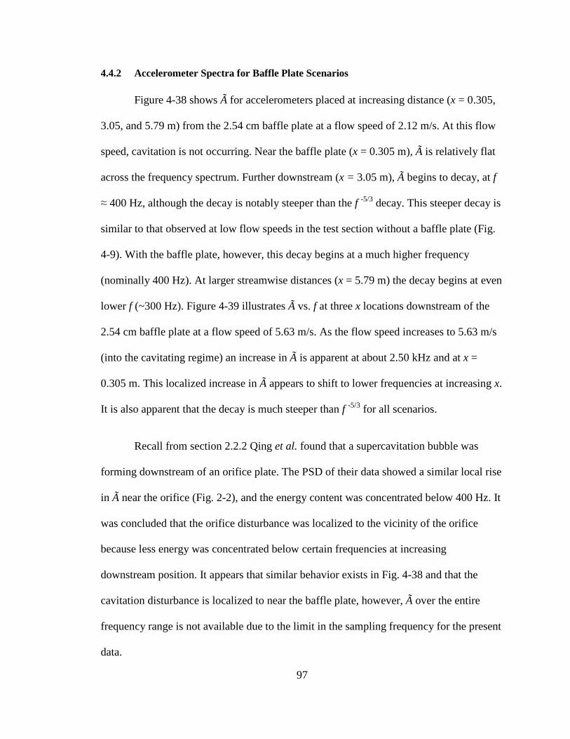
97
4.4.2 Accelerometer Spectra for Baffle Plate Scenarios
Figure 4-38 shows à for accelerometers placed at increasing distance (x = 0.305,
3.05, and 5.79 m) from the 2.54 cm baffle plate at a flow speed of 2.12 m/s. At this flow
speed, cavitation is not occurring. Near the baffle plate (x = 0.305 m), Ã is relatively flat
across the frequency spectrum. Further downstream (x = 3.05 m), Ã begins to decay, at f
≈ 400 Hz, although the decay is notably steeper than the f -5/3 decay. This steeper decay is
similar to that observed at low flow speeds in the test section without a baffle plate (Fig.
4-9). With the baffle plate, however, this decay begins at a much higher frequency
(nominally 400 Hz). At larger streamwise distances (x = 5.79 m) the decay begins at even
lower f (~300 Hz). Figure 4-39 illustrates à vs. f at three x locations downstream of the
2.54 cm baffle plate at a flow speed of 5.63 m/s. As the flow speed increases to 5.63 m/s
(into the cavitating regime) an increase in à is apparent at about 2.50 kHz and at x =
0.305 m. This localized increase in à appears to shift to lower frequencies at increasing x.
It is also apparent that the decay is much steeper than f -5/3 for all scenarios.
Recall from section 2.2.2 Qing et al. found that a supercavitation bubble was
forming downstream of an orifice plate. The PSD of their data showed a similar local rise
in à near the orifice (Fig. 2-2), and the energy content was concentrated below 400 Hz. It
was concluded that the orifice disturbance was localized to the vicinity of the orifice
because less energy was concentrated below certain frequencies at increasing
downstream position. It appears that similar behavior exists in Fig. 4-38 and that the
cavitation disturbance is localized to near the baffle plate, however, Ã over the entire
frequency range is not available due to the limit in the sampling frequency for the present
data.

98
Figure 4-38: à at three x locations downstream of the 2.54 cm baffle plate at a flow speed of 2.12 m/s. The sets of à data have been multiplied by 1000 (x = 0.305 m), 1 (x = 3.05 m), and 0.01 (x = 5.79 m), respectively to differentiate the data sets.
Figure 4-39: à at three x locations downstream of the 2.54 cm baffle plate at a flow speed of 5.63 m/s. The sets of à data have been multiplied by 1000 (x = 0.305 m), 1 (x = 3.05 m), and 0.001 (x = 5.79 m), respectively to differentiate the data sets.
Natural Pipe Response
x = 0.305 m
x = 3.05 m
x = 5.79 m
f -5/3
Natural Pipe Response
x = 0.305 m
x = 3.05 m
x = 5.79 m
f -5/3

99
As previously noted, as the baffle plate hole size decreases, the magnitude of A’
appears very similar to the no baffle plate case. This similarity is also present in Ã. Figure
4-40 shows à at three distances from the 0.159 cm baffle plate (x = 0.305, 3.05, and 5.79
m) at an average flow speed of 2.12 m/s. The roll-off in à is steeper than f -5/3 similar to
the no baffle plate data illustrated in Fig. 4-9 for low flow speeds. There is a slight rise in
à at about 2.50 kHz near the baffle plate (x = 0.305 m), but this vanishes at increasing x.
Figure 4-41 shows à at a flow speed of 5.63 m/s and at the same three x locations.
Comparing this behavior to what is shown in Fig. 4-10, demonstrates that à approaches
an f -5/3 decay at increasing x/D. Near the baffle plate (x = 0.305 m) there is a rise in à at
about 40 Hz that is not present at the other locations, again seeming to indicate that the
disturbance induced by the baffle plate is localized to the baffle plate’s vicinity. This
local rise is similar to what is observed in Fig. 4-39 at the same location. Although
cavitation is not occurring in the 0.159 cm baffle plate, turbulent jets exist and there is
similar behavior in à to the 2.54 cm baffle plate in the vicinity of the plate. As the
distance from the 0.159 cm baffle plate increases, however, the behavior of à becomes
almost indistinguishable from the no baffle plate case.
Figures 4-42 and 4-43 compare à at x = 0.305 m and 5.79 m downstream from all
five baffle plates, at a flow speed of 5.63 m/s. Each à has been multiplied by a factor as
listed in the caption so they are discernable from each other. At x = 0.305 m from the
baffle plates, there is a rise in à at about 2.50 kHz, presumably as a local increase that
will vanish at higher frequencies. Although cavitation is occurring only with the 2.54 cm
and 1.27 cm baffle plates, the increase in à occurs for each baffle plate and indicates that
there is a turbulent disturbance in the vicinity of each baffle plate due to the turbulent

100
jets. The data of Fig. 4-43, at x = 5.79 m from the baffle plate, it shows that for
decreasing baffle plate hole size, the local rise that was noted in Fig. 4-39 either shifts to
higher frequencies or reduces in amplitude, and the decay in à begins to approach the
f -5/3 behavior. It is also interesting to note in Fig. 4-42, at x = 0.305 m from the baffle
plates, although cavitation disappears as the baffle plate hole diameters decrease, there
appears to be little difference in à due to turbulent jets near the baffle plate, which was
also observed by Qing and is mentioned in section 2.2.2.
Figure 4-40: à at a three x locations downstream of the 0.159 cm baffle plate at a flow speed of 2.12 m/s. Sets of à data have been multiplied by 1x10³ (x = 0.305 m), 1 (x = 3.05 m), and 1x10⁻³ (x = 5.79 m), respectively to differentiate the data sets.
Natural Pipe Response
x = 0.305 m
x = 3.05 m
x = 5.79 m
f -5/3

101
Figure 4-42: à at 0.305 m downstream of each of the five baffle plates and at a flow speed of 5.63 m/s. Sets of à data have been multiplied by 1x10⁵ (2.54 cm baffle), 1 x10³ (1.27 cm baffle), 1 (0.635 cm baffle), 1x10⁻⁴ (0.318 cm baffle), and 1x10⁻⁷ (0.159 cm baffle), respectively to differentiate the data sets.
Figure 4-41: à at a three x locations downstream of the 0.159 cm baffle plate at a flow speed of 5.63 m/s. sets of à data have been multiplied by 1x10⁴ (x = 0.305 m), 1 (x = 3.05 m), and 1x10⁻³ (x = 5.79 m), respectively to differentiate the data sets.
Natural Pipe Response
x = 0.305 m
x = 3.05 m
x = 5.79 m
f -5/3
2.54 cm Baffle Plate 1.27 cm Baffle Plate 0.631 cm Baffle Plate 0.318 cm Baffle Plate 0.159 cm Baffle Plate f -5/3
102
In summary far away from the baffle plates and at low flow speeds where
cavitation is not occurring, Ã decays steeper than f -5/3 and is influenced more by the
natural pipe response. As the flow speed increases far away from the non-cavitating
baffle plates, Ã decays nominally as f -5/3 and is influenced very little by the natural pipe
response. Near the baffle plates, independent of cavitation and baffle plate hole size, an
increase in à exists and indicates a turbulent or cavitation disturbance near the baffle
plate. Far away from the baffle plates where cavitation is occurring, a large local rise and
steep decay in à develops that either decreases in amplitude or shifts to higher
frequencies as baffle plate hole size decreases.
Figure 4-43: à at 5.79 m downstream of each of the five baffle plates and at a flow speed of 5.63 m/s. Sets of à data have been multiplied by 1x10⁵ (2.54 cm baffle), 1 x10³ (1.27 cm baffle), 1 (0.635 cm baffle), 1x10⁻² (0.318 cm baffle), and 1x10⁻⁵ (0.159 cm baffle), respectively to differentiate the data sets.
2.54 cm Baffle Plate 1.27 cm Baffle Plate 0.631 cm Baffle Plate 0.318 cm Baffle Plate 0.159 cm Baffle Plate f -5/3

103
5 Conclusion
This thesis presented the results of an experimental investigation to characterize
pipe vibrations induced by turbulent pipe flow. Experiments were conducted using a
water flow loop to address three general phenomena related to pipe vibration: 1) How the
pipe vibration depends on the average flow speed, pipe diameter, and pipe thickness for
an unsupported pipe. 2) How the behavior changes if the pipe is supported at various
clamping lengths. 3) How turbulence generation caused by holed baffle plates influence
the pipe response.
5.1 Vibration Dependence on Fluid Speed and Un-Supported Pipe Parameters
When comparing a power law fit of the average of P’ along the pipe length to Vf,
it was found that P’ scaled nearly as Vf2, with the power from the experimental data
varying less than 5% from an expected value of 2.0. It was determined that A’ for the
unsupported pipe also scaled nearly quadratically with Vf, with an average power over all
the test sections of 2.06. Also, it was shown, doing a similar analysis, that V’ scaled as
Vf1.62, with the power for the V’ relation being about 80% of the A’ value. Put differently,
P’ and A’ are proportional to the dynamic pressure in the pipe; and V’ is proportional to
the dynamic pressure raised to the 0.80 power.
104
It was observed that the magnitude of A’ also varies modestly with inner pipe
diameter (D) and thickness (t). Specifically, A’ was observed to increase as the ratio D/t
increases. However, the dependence on D/t does not appear to be constant with flow rate,
with A’ becoming less dependent on D/t with increasing flow rate.
When computing the PSD of the accelerometer time series data, Ã was found to
be sensitive to the natural pipe response at low flow speeds, with local rises in Ã
corresponding to natural frequencies of the system. The decay of à was also observed to
decay much steeper than f -5/3. This sensitivity to the natural pipe response was observed
to vanish as high flow speeds as the frequency content of à shifted to higher regimes. At
high flow speeds, the pipe vibrations measured by the accelerometers appear to be due to
the local turbulent fluctuations at the pipe wall, which decay as f -5/3.
5.2 Vibration Dependence on Fluid Speed and Clamped Pipe Parameters
Varying the distance between the clamp supports appeared to affect A’ only
modestly. Specifically, A’ was still observed to scale nearly as Vf2 for most of the
clamping distances, with the dependence of A’ on Vf increasing slightly with decreasing
clamping length. However, when the clamping distance became very short, A’ was
observed to scale nearly as Vf3, indicating a greater dependence of A’ on Vf with
decreasing clamping length. This modest clamping length dependence was also observed
to not be constant with flow rate.
Clamping length exhibited a greater influence on V’. It was observed that V’
became less dependent on Vf as clamping length decreased. Also, the magnitude of V’

105
was observed to increase with increasing clamping length, whereas the magnitude of A’
was observed to increase with decreasing clamping length.
5.3 Non-Dimensionalization of A’
When comparing the non-dimensionalized pipe wall acceleration (A*) to the non-
dimensional parameters Re, t*, L*, E*, ρ*, and ω*, it was found that A* was weakly
dependent on all of them except ρ*. This was in good agreement to a parallel numerical
study performed by Shurtz 24. This strong dependence on ρ* resulted in the scaling
relationship, A’~ Vf2/t*ρ*. This scaling relationship is a first order estimate of the expected
level of pipe vibration in a long or unsupported pipe.
Where the clamping support was long, Ã was observed to be very similar to the
unsupported case. However, Ã was observed to be more sensitive to the natural pipe
response when clamping was short, even at high fluid speeds.
5.4 Baffle Plate Influence on Pipe Response
It was found that placing baffle plates into the flow would induce turbulence
downstream of the baffle plate. For large baffle plate hole size cavitation existed at high
fluid speeds. Cavitation would cause the magnitude of A’ to increase by up to 300 times.
As the baffle plate hole size decreased, it was observed that the fluid speed at which
cavitation would initiate would increase to greater values. Cavitation was not prevalent at
all with baffle plate hole sizes smaller than 0.635 cm. Further, it was observed that as the
baffle plate hole size decreased, A’ would approach magnitudes shown with the no baffle

106
plate baseline. A’ was also observed to decay to baseline levels as the distance from a
non-cavitating baffle plate increased.
Away from a non-cavitating baffle plate, the decay of à approaches the expected
f -5/3 power law relation. Cavitation was observed to cause a local rise in à that either
shifts to higher frequencies or decreases in magnitude as the baffle plate hole size
decreases, with cavitation ceasing completely with the small diameter baffle plates. Near
each baffle plate, a rise in Ã, regardless of cavitation, indicates that a turbulent
disturbance exists at the plates.
5.5 Recommendations
This thesis presented the results of an experimental study with the purpose of
characterizing turbulence induced pipe wall vibrations. Although these results were
compared to the results of other researchers, namely Pittard et al., this thesis examined
only one pipe material (PVC), one fluid (water), and two standard thicknesses of pipe
(schedules 40 and 80). Future studies should employ more pipe materials (such as
aluminum or stainless steel), a fluid with a different density (such as air), and an extended
range of pipe schedules (such as schedules 10 and 160).
Also, great care should be taken when drilling pressure taps. It was noted that
about 72 % of the uncertainty in the pressure measurements were due to burr effects.
These effects made more than general comparisons of wall pressure fluctuations between
tap locations and test sections suspect. This uncertainty also obscured comparisons
between the pressure measurements and acceleration measurements.

107
Finally, it is recognized that conducting the several experiments necessary to
characterize the fluid induced pipe vibrations are limited because of the limited number
of elements that can varied and due to cost both in time and money. Therefore, the
experimental results presented in this thesis can be used as validation for numerical
studies similar to the study completed by Shurtz 24. The advantage of a numerical study is
that it gives the ability to change the fluid and pipe parameters with relative ease
5.6 Publications
A publication based on part of the work presented in this thesis has been
presented at the 2009 ASME fluids engineering summer meeting (FEDSM2009). This
work presents a comparison between the 10.16 cm and 7.62 cm test sections and the
results presented by Pittard et al. 2. Correlations that collapsed the data from both sources
were formulated. Subsequent journal publications of the results will be pursued.

108

109
6 References
1. Awawdeh, A., Bukkapatnam, S.T.S., Kumara, S.R.T., et al., “Wireless sensing of Flow-Induced Vibrations for Pipeline Integrity Monitoring,” IEEE SAM 06, Boston, July 2006.
2. Pittard, M.T., Evans, R. P., Maynes, D., Blotter, J., “Experimental and Numerical Investigation of Turbulent Flow Induced Pipe Vibration in Fully Developed Flow,” Review of Scientific Instruments, Vol. 75, Number 7, July 2004, pp 2393-2401.
3. National Transportation Safety Board, “Pipeline Accident Brief,” NTSB/PAB-01/02, Pipeline accident number: DCA-00-MP-004, May 3, 2001.
4. Figliola, R.S., Beasley, D.E., Theory and Design for Mechanical Measurements, Second Edition, John Wiley and Sons, Inc., 1995.
5. Evans, R.P., Blotter, J.D., Stephens, A.G., “Flow Rate Measurements Using Flow-Induced Pipe Vibration,” Transactions of the ASME, Vol. 126, March 2004, pp 280-285.
6. Kim, Y.K., Kim, Y.H., “A Three Accelerometer Method for the Measurement of Flow Rate in Pipe,” Journal of the Acoustical Society of America, Vol. 100, Number 2, Part 1, August 1996, pp 717-726.
7. Genscape Inc. Website: http://www.genscape.com/pages.php?uid=2
8. Blevins, R.D., “Flow-Induced Vibration in Nuclear Reactors; a Review,” Progress in Nuclear Energy, Vol. 4, 1979, pp 25-49.
9. Paidoussis, M.P., “Fluidelastic Vibratio of Cylinder Arrays in Axial and Cross Flow: State of the Art,” Journal of Sound and Vibration, Vol. 76, Number 3, 1981, pp 329-360.
10. Reavis, J.R., “Vibration Correlation for Maximum Fuel-Element Displacement in Parallel Turbulent Flow,” Nuclear Science and Engineering, Vol. 38, 1969, pp 63-69.

110
11. Burgreen, D., Byrnes, J.J., Benforado, D.M., “Vibration of Rods Induced by Water in Parallel Flow,” Transactions of the ASME 80, 1958, pp 991-1003.
12. Bernard, P.S., Wallace, J.M., Turbulent Flow Analysis, Measurement and Prediction, John Wiley and Sons, Inc., 2002.
13. Saddoughi, S.G., “Local Isotropy in Complex Turbulent Boundary Layers at High Reynolds Number,” Journal of Fluid Mechanics, Vol. 348, 1997, pp 201-245.
14. Lysak, P.D., “Modeling the Wall Pressure Spectrum in Turbulent Pipe Flows,” Transactions of the ASME, Vol. 128, March 2006, pp 216-222.
15. “Kolmogorov Cascade,” Encyclopedia of Non-Linear Sciences.
16. Caillaud, S., Gibert, R., Moussou, P., Cohen, J., Millet, F., “Effects on Pipe Vibrations of Cavitation in an Orifice and in Globe-Style Valves,” Proceedings of Pressure Vessels and Piping Conference, July, 2006.
17. Qing, M., Jinghui, Z., Yushan, L., Haijun, W., Quan, D., “Experimental Studies of Orifice-Induced Wall Pressure Fluctuations and Pipe Vibration,” International Journal of Pressure Vessels and Piping, Vol. 83, 2006, pp 505-511.
18. Qing, M., Jinghui, Z., “Orifice-Induced Wall Pressure Fluctuations and Pipe Vibrations: Theory and Modeling of Fluid Excitation,” Flow Turbulence and Combustion, Vol. 79, 2007, pp 25-40.
19. Moussou, P., “An Attempt to Scale the Vibrations of Water Pipes,” Transactions of the ASME, Vol. 128, November 2006, pp 670-676.
20. Maynes, D., “Turbulence Induced Vibration in Straight Pipe Flow Considerations.”
21. Munson, B.R., Young, D.F., Okiishi, T.H., Fundamentals of Fluid Mechanics, Fifth Edition, John Wiley and Sons, Inc., 2006.
22. Tropea, C., Yarin, A.L., Foss, F.F., Springer Handbook of Experimental Fluid Mechanics, 2007, pp 180-185.
23. Brown, J.W., Churchill, R.V., Fourier Series and Boundary Value Problems, Sixth Edition, McGraw Hill, 2001.
24. Shurtz, T.P., Analysis of Induced Vibrations in Fully-Developed Turbulent Pipe Flow Using a Coupled LES and FEA Approach, Brigham Young University, Provo, UT, USA, Master’s Thesis, 2009.

111
Appendix A: MatLab rms Code
The following is the MatLab code was used to calculate the rms values of the time
series data that was collected.
clear; close; clear filename n = 22; % number of files % %Filename Convention is: D:\Pipe diameter and schedule\Diameter of %developing region if different than 4 inch\Which baffle plate was inserted %and the units acceleration is measured in\Which LabView VI was used\Which %experiments were run and support location\Accelerometer and Pressure %transducer location\Pressure transducer x/D %location\PipeDiameter_PipeSchedule_PumpSpeed_0001.txt intro = 'D:\2 inch Schedule 40\2 inch Developing Region\No Baffle Plate Accel in Gs\New VI\ApPp_xod_no sup\Same Location Opposite Sides P1A1_West_P2A2_East\PA_18ft\2in40_'; % % samples = 50000; time = 1/5000; %Structures were used for ease of manipulating the data. for i = 1:n istring = int2str((i-1)*2); if 2*(i-1) < 10 filename(i).name = strcat(intro,'0',istring,'Hz_0001.txt'); else filename(i).name = strcat(intro,istring,'Hz_0001.txt'); end Data = load(filename(i).name); % Picks the corresponding data from the following columns. filename(i).tyme=Data(:,1); filename(i).ua1=Data(:,2); filename(i).ua2=Data(:,3);

112
filename(i).v1=Data(:,4); filename(i).v2=Data(:,5); filename(i).disp1=Data(:,6); filename(i).disp2=Data(:,7); filename(i).flow=Data(:,8); filename(i).p1=Data(:,10); filename(i).p2=Data(:,11); filename(i).pdif=Data(:,12); filename(i).p1f=Data(:,13); filename(i).p2f=Data(:,14); filename(i).pdiff=Data(:,15); % Calculates the RMS values filename(i).ua1rms=sqrt(mean(filename(i).ua1.^2)); filename(i).ua2rms=sqrt(mean(filename(i).ua2.^2)); filename(i).vel1rms1000=sqrt(mean(filename(i).v1.^2))*1000; filename(i).vel2rms1000=sqrt(mean(filename(i).v2.^2))*1000; filename(i).disp1rms1000=sqrt(mean(filename(i).disp1.^2))*1000; filename(i).disp2rms1000=sqrt(mean(filename(i).disp2.^2))*1000; filename(i).flowrms = sqrt(mean(filename(i).flow.^2)); filename(i).p1rms = sqrt(mean(filename(i).p1.^2)); filename(i).p2rms = sqrt(mean(filename(i).p2.^2)); filename(i).pdifrms = sqrt(mean(filename(i).pdif.^2))/sqrt(2); filename(i).p1frms = sqrt(mean(filename(i).p1f.^2)); filename(i).p2frms = sqrt(mean(filename(i).p2f.^2)); filename(i).pdiffrms = sqrt(mean(filename(i).pdiff.^2))/sqrt(2); i end % Builds a table of the rms values. RMS = zeros(n,13); for i = 1:n RMS(i,1) = filename(i).ua1rms; RMS(i,2) = filename(i).ua2rms; RMS(i,3) = filename(i).vel1rms1000; RMS(i,4) = filename(i).vel2rms1000; RMS(i,5) = filename(i).disp1rms1000; RMS(i,6) = filename(i).disp2rms1000; RMS(i,7) = filename(i).flowrms; RMS(i,8) = filename(i).p1rms; RMS(i,9) = filename(i).p2rms; RMS(i,10) = filename(i).pdifrms; RMS(i,11) = filename(i).p1frms; RMS(i,12) = filename(i).p2frms; RMS(i,13) = filename(i).pdiffrms; end

113
Appendix B: MatLab à Code
The following code was used to calculate the normalized PSD of the pipe
acceleration time series (Ã).
clear; %close; n = 24; % number of files %Naming Convention: E:\Pipe diameter and schedule\Baffle plate case and %units acceleration is measured in\Which LabView VI was used\Wall support %locations_Accelerometer % locations\PipeDiameterPipeSchedule_PumpSpeed_0001.txt intro = 'E:\4 inch Schedule 40\No Baffle Plate Accel in Gs\New VI\Quarter Wall Support_A1_0.125_A2_0.0625\4in40_'; samples = 50000; time = 1/5000; sampfreq = 5000; for i = 8 for j = 1:5 istring = int2str(2*(i-1)); if 2*(i-1) < 10 filename(i).name = strcat(intro,'0',istring,'Hz_0001','.txt'); else filename(i).name = strcat(intro,istring,'Hz_0001','.txt'); end Data = load(filename(i).name); filename(i).tyme=Data(:,1); % Breaks data into 2 second chunks filename(i,j).ua1=Data(10000*j-9999:10000*j,2); % Calculates RMS values of the chunks filename(i,j).ua1std=std(filename(i,j).ua1); filename(i,j).ua1norm = filename(i,j).ua1/filename(i,j).ua1std;

114
% FFT of the acceleration % Takes the FFT of each chunk filename(i,j).afft = abs(fft(filename(i,j).ua1norm)); % Calculates the PSD of each chunk. filename(i,j).apsd = (filename(i,j).afft).^2; freq = 0:1/2:5000/2-1/2; % Averages the FFT of each chunk filename(i).afftavI = mean(filename(i,j).afft,2); filename(i).afftav = filename(i).afftavI(1:5000); % Averages the PSD of each chunk filename(i).apsdavI = mean(filename(i,j).apsd,2); filename(i).apsdav = filename(i).apsdavI(1:5000); filename(i).apsdavnorm = filename(i).apsdavI(1:5000)/(length(filename(i).apsdav))^2; end % Parseval's Theorem, integrating the PSD and dividing by the length of % the PSD. This normalized integral should be equal to 1. filename(i).IntPSDav = sum(filename(i).apsdavI)/((length(filename(i).apsdavI))^2); Parseval = filename(i).IntPSDav end % Plots the PSD figure loglog(freq(1:5000),filename(8).afftav(1:5000),'r-') hold on loglog(freq(1:5000),filename(8).apsdav(1:5000),'g-') % loglog(freq2,respfftave(1:size(freq2,1)),'b-') hold off
115
Appendix C: Pipe Scaling Estimations
The following document outlines how pipe displacement, velocity, and
acceleration fluctuations are expected to scale with various fluid and pipe characteristics.
The first segment of the document assumes elastic behavior in bending of the pipe due to
unsteady loading. The second segment assumes that the pipe is constrained from bending,
as a buried pipe. This document was developed by Maynes 21.

116
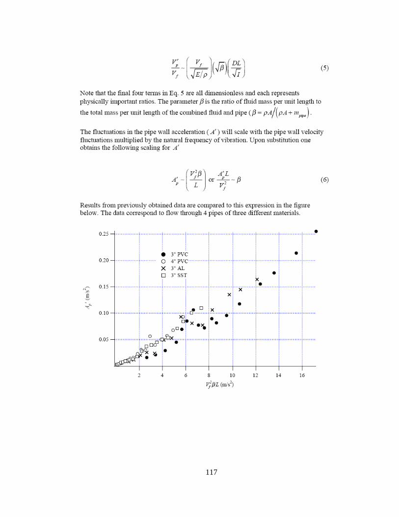
117

118
119

120