Experimental estimation and CFD validation of an Electro Submersible Pump’s (ESP)

curve for two fluids with different viscosities

Santiago Becerra Plaza

201423134

Universidad de Los Andes

Chemical Engineering Department

1. Nomenclature

𝐵 Parameter for the hydraulic institute method

𝐶𝐻 Head correction factor 𝐶𝑄 Flow rate correction factor

𝐹 External forces

𝑔 Gravity

𝐻 Head

𝐻𝐵𝐸𝑃−𝑤 Water head at best efficiency point

𝐻𝑣𝑖𝑠 Viscous fluid head

𝐻𝑤 Water head

𝐼 Identity matrix

𝑁 Frequency of the motor

�̅� Mean pressure

𝑝𝑖𝑛 Pressure at the inlet

𝑝𝑜𝑢𝑡 Pressure at the outlet

𝑄𝐵𝐸𝑃−𝑤 Water flow rate at best efficiency point

𝑄𝑣𝑖𝑠 Viscous fluid flow rate

𝑄𝑤 Water flow rate

�̅� Mean velocity

𝑉𝑣𝑖𝑠 Cinematic viscosity

𝜌 Density

𝜏 Viscous stress tensor

𝜏𝑡 Reynolds stress tensor

2. Objectives

2.1. General Objective

To study the behavior and performance of an Electro Submersible Pump (ESP), considering water

and mineral oil as working fluids.

2.2 Specific Objectives

• To build an appropriate experimental set-up where an ESP’s operating conditions can be

analyzed.

• To construct a CFD model that correctly predicts the head curve of the ESP by estimating

the behavior of the flow inside the system considered.

• To validate the results obtained with the CFD model by comparing numerical results with

experimental data. To compare the proposed method for estimating head degradation with

well-known graphical methods.

3. Introduction

When the internal pressure in oil wells is too low to generate the flow needed,

artificial lift methods are used for production. In the early stages, oil wells have enough

pressure to allow fluids to get to the surface but with the passage of time the flow to the

surface may stop. This can occur for two reasons: i) an increase in the lift required to move

the well stream or ii) a decrease in the bottom hole pressure. In the first case, an increase

in flow resistance can be caused by a greater density of the flowing fluid because of a

decrease in gas production or a mechanical problem in the system[1]. The second case

happens naturally after removing fluids from the reservoir.

Artificial lift is the addition of energy to the flow stream to increase flow rate in these

situations [2]. It can be created with high pressure injection of gas or with a pump. Gas

lifting can be done through a constant injection of gas at some downhole points, which

reduces the viscosity of the fluids in the well and therefore, the flow resistance, or by an

intermittent injection, enough air is injected periodically in the tubing to lift a column of

fluid[1]. On the other hand, pumping methods have a wide variety of options to choose

from, including jet pumps, progressive cavity pumps, beam pumps hydraulic piston pumps

and electrical submersible pumps[2].

An Electrical Submersible Pump (ESP) is a centrifugal pump consisting of a

multistage arrangement (each containing a diffuser-impeller pair), a submerged motor,

wiring run from the surface and a gas or solid separator may be included, used to reduce

wear on moving parts (Figure 1). This units are used onshore as well as offshore,

characterized for their ability to produce high volumetric flows, at the time they started to

be used at oil wells they could produce up to three times the volumetric flow of a rod

pump[1].

Figure 1. Cross section of the ESP, where the four stages can be seen. In addition, parts like the check valve, the inlet, outlet and shaft are also shown.

Advantages of ESPs include a relatively high efficiency (approximately 50%) for productions

over 1,000 bpd, silent operation, minimal space requirements, easy to perform corrosion

treatments and a rate of production of up to 30,000 bpd for medium depths [1]. In contrast, these

units are sensible to solid particles, and require a reliable source of power of relatively high voltage,

they are sensible to high temperatures and for high concentrations of gases the pump experiences

a condition known as Gas Locking, were the air generates a blocking on the pump [3].

Any problem that requires intervention inside the equipment installation is of serious

matter, given that the cost of this operation could surpass the initial cost of the equipment [2]. As a

result, there has been a growing interest around studying ESPs. Effects of the harsh environments

in which these pumps operate have been evaluated experimentally.

Lea and Bearden (1982) tested three different pumps by changing the gas volume fraction

(GVF) of the system until pump failure due to gas locking occurred [4]. In between the pumps that

were chosen, Lea and Bearden were able to evaluate mixed flow in addition to radial flow impellers

while working with diesel-CO2 and water-air mixtures. They found that mixed flow impellers work

better with gas liquid mixtures and increasing pressure at pump inlet lowers head degradation. Cirilo

(1998) studied the effects of frequency variation, number of stages, gas volume fraction on the

performance of three different ESPs working with water-air mixture [5].

Pessoa et al. (1999) performed similar tests but with crude oils, to determine the amount of

gas an ESP with axial flow could handle, while also trying to specify the amount of GVF to cause a

gas lock in the system, which was found to be up to 50 % for the lightest oil [6]. Pessoa and Pardo

(2003) studied not only gas locking but also surging by gathering data from every stage of a 22-stage

ESP working with an air-water mixture [7]. Given that ESPs also have to handle multiple fluids with

different viscosities, Bulgarelli (2017) collected data from an ESP working with a water-oil mixture,

varying the concentration of water to calculate the point of inversion of the emulsion formed in the

system. It was found that water as the continuous phase improves overall efficiency of the system

when compared to oil as the continuous phase [8].

To better understand the performance of ESPs, observation of flow behavior started to

become more relevant. Lopez and Kenyery (2007) focused on analyzing the bubble size of air at the

pump’s inlet through digital images taken from short videos. They found that the only factor

affecting bubble size diameter is pressure at the pump’s inlet. In addition, rising the pressure at the

inlet can only lessen pressure degradation to a certain extent [9]. Gamboa and Prado (2009) studied

the behavior of the gas pockets formed in a water-air mixture flow through an ESP, for his

experiments he used a two-stage prototype of an ESP made of transparent acrylic. The effect of gas

density and surface tension on flow behavior was observed as well as the formation of gas pockets

that cause surging [10]. Perissinotto (2017) conducted a similar study, he made an experimental

visualization and analysis of oil droplets inside a water flow through an ESP with the help of a high

speed camera [11].

Because of the high impact ESP performance has on production costs in the oil industry,

studies have been carried to design methods to predict how the ESP’s efficiency and head will vary

regarding the change of operating conditions. Turpin (1986) proposed a correlation to predict head

degradation at flow rates higher than that of the best efficiency point, considering the free gas to

liquid ratio, pump intake pressure and flow rate [12]. With the same data Sachdeva (1988)

developed a dynamic model based on a model used for pumps in the nuclear industry[13]. Even

considering the difference between nuclear and petroleum industry pumps, the biggest drawback

was the model’s complexity.

For this reason, Sachdeva (1992) developed a simpler model to estimate pressure rise per

stage, correlating the pressure increase per stage, pump inlet pressure, pump inlet void fraction and

the liquid flow rate [14]. Zhou (2010) worked on Sachdeva’s simplified model, adjusting some terms

to propose a new model to estimate head degradation -which had a better prediction for the data

taken by Lea and Bearden model- at the same time presented models for finding the critical point

of gas-liquid operations[15]. The critical point is the maximum amount of GVF allowed in the system

before surging occurs. Estimating the critical point is of great importance when working gassy wells,

as a result many have proposed models to predict the critical point of an ESP [5, 12, 16, 17].

Other methods have been developed for what accounts to fluid viscosity head degradation,

where no GVF is considered. Stepanoff (1948) proposed a general model considering general shock

and friction losses [18]. Gülich (2014) developed another analytical model considering losses caused

by leakage, disk friction, impeller friction, mechanical efficiency and slippage [19]. Viera (2014)

studied the effects of shock, friction, recirculation, diffuser and disk pressure losses on calculations

for head degradations due to fluid viscosity [20]. Impeller and disk friction were the had the largest

impact on head degradation. Simpler methods have been proposed. The Hydraulic Institute

Standards, those published in 2004, included a graphical method to calculate the head curve of a

rotodynamic pump knowing the fluids viscosity and the head curve for water [21]. Later, KSB (2005)

broaden the range of said method by including some correction factors based on the specific speed

of the pump [22].

As an alternative to experimental analysis, numerical methods can be used to analyze the

behavior of internal flow of equipment together with an estimation of the pumps performance.

Rising computer power and accuracy improvement of numerical methods have helped them

become a competitive tool for industrial applications. Computational Fluid Dynamics (CFD) has

successfully contributed to the enhancement of turbomachinery design [23]. Many researches have

started to use CFD as an approach to flow analysis. Caridad and Kenyery (2004) simulated one blade

of an ESP mixed flow impeller working with a water-air mixture with the objective of analyzing gas

phase distribution [24]. Stel (2014) studied the effects of fluid viscosity on the head curve of an ESP

by simulating a three-stage mixed flow ESP, where -to reduce computational costs- only one seventh

of each diffuser-impeller pair was considered. Flow on diffuser could be seen affected by suction

head of downstream impellers, hence the importance of simulating various pump stages [25, 26].

Zhu et al. (2016) tested various fluids oils different viscosities inside a seven-stage mixed

flow ESP. A CFD analysis of all 7-stages was conducted but the simulation domain undertook only

one passage through each piece of the stage, impeller and diffuser. An over estimation of the head

curve mad by the CFD analysis was detected along with certain linearity in some head curves for the

high viscosity fluids, which could indicate laminar flow[27]. Ofuchi et al. (2017) conducted a CFD

analysis of a three-stage mixed flow ESP but, unlike others, his simulation domain covered the hole

impeller-diffuser geometry of each stage. A direct dependency of friction losses on the Reynolds

number was stated, together with an effect of recirculation in the diffuser on downstream impellers

turbulence[28]. Babayigit et al. (2017) studied the effects of leakages and balance holes on a radial

flow of a centrifugal pump, improving considerably accuracy in pump performance calculation at

the same time computational costs are significantly increased [29].

This study addresses pump degradation caused by fluid viscosity, analyzing a numerical

method (CFD) and a more common graphical method as an approach to predict pump degradation.

The behavior of the fluid inside a 4-stage radial flow ESP is simulated. Additionally, the calculations

with the empirical approach mentioned before and a complete comparison with the data obtained

helps to indicate the improvements with the proposed method. Two different fluid viscosities are

going to be tested at a constant rotational speed, to cover some of the industrial problems that can

occur during normal operation of wells.

4. Materials and Methods

4.1 Experimental set-up

The pump used is an electrical submergible pump from Franklin Electric with model number

20FA05S4. Said ESP has four stages, works with radial flow and is driven by a 0.5 hp monophasic

motor. Fluids used are water and mineral oil with their properties shown in (Table 1). In the

experiments the head curve of the curve of the pump is measured by measuring the pressure at the

pump outlet for 0, 5, 7, 10, 15, 20 and 25 gpm. These flow rates are the same flow rates for which

the manufacturer gives the head of the pump produces, the same flow rates are used in this study

to properly compare the head curve obtain experimentally and the one given by the manufacturer.

Additionally, rotating rate of the pump is measured with a digital tachometer in each experiment to

have the required parameters at the time the CFD analysis. Frequency is measured with a digital

tachometer.

Table 1 Fluids used in this study and their properties at 25°C.

Name Density (kg/m3) Dynamic viscosity (Pa*s)

Water 997.561 0.001 Mineral Oil 863.104 0.031

The idea of the experimental set-up is to allow the ESP to pump water from the same site it

is extracting it from, that so to operate the unit several times without recurring to extra fluid cost.

Another design requirement is the ability to measure the ESP’s rotation rate. The difficulty being

that as the unit is submerged, there is no practical way to attach a measuring device to the motor

or shaft. Therefore, a unique part is design and manufactured to extend the shaft of the system

(Figure 2), that way being able to measure the rotational frequency of the impellers with any

tachometer.

Figure 2 Design of the shaft extension used to measure frequency of the motor.

Looking to reduce the space occupied as much as possible, the design is made to have all its

parts inside the same place where the fluid is being stored (Figure 3). A 250-liter water storage tank

is used as the containment for the set-up. To sustain the vertical position of the ESP a structure

made from iron angles is manufactured. The design of the structural components is made so the

bearings for the shaft extension can be properly installed. Given that iron corrodes with ease, paint

is applied over the material to ensure its durability while working with water. As a method of

determining the level inside the tank, a measuring tape is attached inside of the storage equipment.

Figure 3 Initial sketch for the experimental set up. It outlines the main parts of the set up and shows the solid structure designed to give support to the system.

Pressure is registered with a Sper Scientific wide range pressure meter and a 725 psi Sper

Scientific transducer. The pressure transducer is located next to the ESP’s outlet, to avoid losses

from fittings. For flow rate readings, a Hedland Ez-view oil flow meter with a range from 4 to 28

gpm. Using a positive displacement flow meter, as the one chosen for this study, allows the use of

different fluids with different densities and viscosities while being economically accessible. Hedland

provides correction factor for fluid with different viscosities at which the product is calibrated, it can

be found in the user manual [30]. The digital tachometer used in this study is a Protmex MS6208A.

A gate valve is used to vary flow rate through the system. To avoid leakage where the shaft extension

comes out of the piping, a single spring mechanical seal is installed. The experimental set-up is

shown on Figure 4.

earingsP piping

alve

low meterPressure sensor

Pump

otor

Sha extension

Iron structure

Figure 4 Image of the experimental set-up.

4.2 Numerical study

4.2.1 Geometry Model

A 3D CAD model of the inside of the pump is created using Autodesk Inventor Professional

2017 and AutoCAD 2018. The inside of the pump consists of: (i) four stages each with a diffuser to

redirect flow towards the next stage and an impeller, (ii) a shaft and (iii) a structure part that holds

everything together. The ESP is disassembled and taken apart, each part is carefully measured with

a caliper to have precise dimensions for the 3D CAD model.

Some parts require more detail, especially when they are composed of complex curves. This

is the case of the volute and the impeller. A picture is taken for each of these parts in a way that the

complex curve behavior is captured. Then, the photo is imported into an AutoCAD file, where a

spline is traced along the complex curve. For scaling purposes, a circle is traced along the

circumference of the part, be that the stage casing (which contains the diffuser) or the impeller.

Afterwards, the coordinates of each point are transferred to a Microsoft Excel file, here the

coordinates of the splines points are scaled to their value in millimeters using the diameter of the

circle traced over the picture and the radius measured with the caliper. With the new coordinates

the splines are built in Autodesk Inventor to construct the stage casing and the impeller (Figure 5).

Figure 5. Demonstration of the steps taken to build the parts which involved the modelling of complex curves.

Once the impeller and diffuser are constructed inside Autodesk inventor, the stage is

assembled (Figure 6). With this assembly and the remaining parts, the 4-stage geometry is put

together. The extent of this study does not consider leakage effects or small passages in the pump

interior, like the one showed on Figure 1. With the 3D model design, the internal volume of the ESP

is extracted to make what is the domain of the CFD analysis, as shown in Figure 7.

Figure 6 shows how the stage is assembled and a cross section, to illustrate the geometry.

Figure 7 shows the complete internal volume of the ESPs 3D model. The regions used in the creation of the mesh are outlined.

4.2.2 Mesh structure

STAR-CCM+ has various options for creating the grid, depending on the type of cells and

type of geometry it has. For this study the three following procedures are chosen for mesh creation:

surface remesher, polyhedral mesher and prism layer mesher. The surface remesher optimizes the

volumes surface for the volumetric meshers, it addequates surfaces for the prism mesher and treats

initial tellesatelation. The polyhedral mesher alleviates computational time by reducing cells almost

five times aas those generates by a tetrahedral mesher. It is great for complex geometries and it

does not require the amount of surface preparation that a tetrahedral mesher needs. The prism

layer mesher is used for improved accuracy for near wall flow. It not only improves wall density but

also provides a better cross stream resolution[31].

Defining the parameter with which the grid is going to be generated depends on the

turbulence model chosen for the simulation. To obtain a good grid over the wall surfaces a total of

10 prism layers and a thickness of 20% the base size is used as a parameter for the prism layer

mesher, as a good balance between mesh density, accuracy and computational requirements. It is

important to define the thickness of the prism layer as a relative value of the base size, to develop

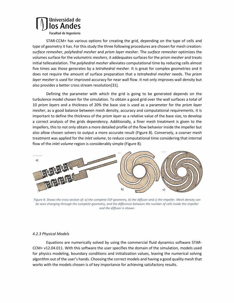
a correct analysis of the grids dependency. Additionally, a finer mesh treatment is given to the

impellers, this to not only obtain a more detailed profile of the flow behavior inside the impeller but

also allow chosen solvers to output a more accurate result (Figure 8). Conversely, a coarser mesh

treatment was applied for the inlet volume, to reduce computational time considering that internal

flow of the inlet volume region is considerably simple (Figure 8).

Figure 8. Shows the cross section of: a) the complete ESP geometry, b) the diffuser and c) the impeller. Mesh density can be seen changing through the complete geometry, and the difference between the number of cells inside the impeller

and the diffuser is shown.

4.2.3 Physical Models

Equations are numerically solved by using the commercial fluid dynamics software STAR-

CCM+ v12.04.011. With this software the user specifies the domain of the simulation, models used

for physics modeling, boundary conditions and initialization values, leaving the numerical solving

algorithm out of the user’s hands. Choosing the correct models and having a good quality mesh that

works with the models chosen is of key importance for achieving satisfactory results.

It is first required to determine a method for simulating simultaneous rotational and

stationary components. CFD codes offer different approaches to resolve turbomachinery problems.

Some options consider the position of the rotatory parts, thus displacing mesh vertices in real time

and making the simulation an unsteady problem. Another more common method is using a Moving

Reference Frame (MRF). In the MRF method, the equations for the fluid surrounding the impeller

are solved in a rotating reference frame without changing the geometry, meaning the rotational

region is kept at a fixed position [23]. As a result, the simulation can be considered in a steady state,

lowering computational costs significantly.

Next is deciding how the momentum and continuity equations are going to be solved. Since

the experimental set-up was run at a constant temperature with Newtonian fluids, density and

viscosity are taken as constant values. The segregated solver is recommended for this type of

incompressible flows.

For the turbulence model, it is known that there is no significant difference between using

k-ε or k-ω turbulence models, which are two of the most common turbulence models for

turbomachinery [32]. The k-ε model for all y+ was chosen to simulate turbulence, given it provides

a good compromise between robustness, computational cost and accuracy. This model is also

appropriate in showing complex recirculation scenarios, which can occur inside the impellers

passages inside the pump. It is recommended to use the realizable k-ε turbulence model, because

its results are equal or better than the standard k-ε model [29,32].

The governing equations are continuity and momentum for the Reynolds-Averaged Navier-

Stokes:

𝜕𝜌

𝜕𝑡+ ∇ ∙ (𝜌�̅�) = 0

(1)

𝜕

𝜕𝑡(𝜌�̅�) + [∇ ∙ 𝜌�̅��̅�] = −∇�̅�𝑰 − [∇ ∙ (𝝉 + 𝝉𝒕)] + 𝐹

(2)

Convergence is considered in this study as there is no change in residuals, thus a constant

output of the results. After achieving convergence, the head generated by the pump is calculated,

using the output and inlet boundaries as a reference. Head at the inlet and outlet are calculated,

followed by a subtraction between both values. In this study head is calculated as:

𝐻 =𝑝𝑜𝑢𝑡 − 𝑝𝑖𝑛

𝜌𝑔 (3)

4.2.4 Initial and boundary conditions

As said before, the approach to simulating rotation in this analysis is the MRF method. Four

regions are specified to have a rotational reference frame, each of which is located between the

stage inlet and the beginning of the diffuser, thus containing the impeller (Figure 7). At the inlet of

the 4-stages a mass flow inlet is specified, where the value changes depending on the volumetric

flow rate for which the head is going to be calculated. At the outlet of the geometry a flow-split

outlet with a ratio of one is specified as the boundary condition.

For pressure initial values the gauge pressure is used, this case being 0.0 Pa. A value of 0

m/s was specified as the initial condition for velocity, because it was found that it helped

convergence for all the simulations. The initial values for turbulence intensity, length scale and

velocity inlet were found to give a faster convergence when left at the values recommended by

STAR-CCM+.

4.3 Correlation model

To compare the prediction of head degradation calculated by CFD methods a more classical

approach is also used. Using the 2010 standards of the Hydraulic Institute, the performance of a

rotodynamic pump working with fluids with different viscosity than water is calculated [33]. The

method is based on a Reynolds number adjusted for specific speed, called parameter B. This

parameter has been statistically curve-fitted to a body of test data. First, the parameter B need to

be calculated:

𝐵 = 16.5

(𝑉𝑣𝑖𝑠0.5)(𝐻𝐵𝐸𝑃−𝑤

0.0625 )

(𝑄𝐵𝐸𝑃−𝑤0.375 )(𝑁0.25)

(4)

For this method the best efficiency point is taken at 20 gpm, since the manufacturer states

that this ESP is designed to work at that flow rate. The following step is to calculate the correction

factor for flow:

𝐶𝑄 = 2.710.165(log10 𝐵)3.15 (5)

𝑄𝑣𝑖𝑠 = 𝐶𝑄𝑄𝑤

(6)

Then the correction factor for head can be calculated:

𝐶𝐻 = 1 − [(1 − 𝐶𝑄) (

𝑄𝑤

𝑄𝐵𝐸𝑃−𝑤)

0.75

]

(7)

𝐻𝑣𝑖𝑠 = 𝐶𝐻𝐻𝑤

(8)

With the correction factors the corresponding viscous quantities can be estimated. The

viscous quantities predict the behavior of the pump at the same flow rate as that of water but with

a fluid with different viscosity.

5. Results and discussion

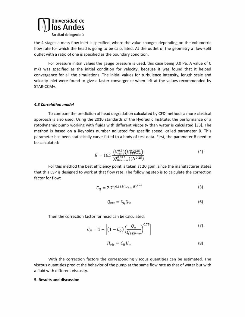
5.1 Mesh dependency

Various grids are tested at an arbitrary flow rate, 10 gpm, to compare their error with the

experimental data. All the parameters inserted in the three meshers used to create the grid are

specified relative to the base size of the mesh. Starting from 7.15 mm the base size value is gradually

decreased until the error is virtually constant. As seen in Figure 9 and Table 2, choosing a base size

of 2.5 mm guarantees that having a finer mesh will not lower the error in calculation, hence the

independency of the results from the grid chosen.

Figure 9 Graphical representation of the effect of number of elements in a grid on the percentage of error of the estimated head through the CFD analysis. The base size used for each mesh is shown in Table 2.

Table 2 Shows the base size used in each mesh. Parameters used on the mesh operations are relative to the base size.

Mesh Number Base size [mm]

1 7.15

2 5.50

3 4.25

4 3.25

5 2.50

6 1.90

7 1.50

5.2 Head curve and degradation performance

It can be seen on Figure 10 that the manufacturers head curve over specifies the

performance of the pump for low and high flows. At flow rates of 10 and 15 gpm the specification

of the head given by the pump is accurate, but there is a significant difference at the other flow

rates. The head curve obtained from the experimental results gets to be more than 13% for some

flows. Furthermore, the behavior observed by the manufacturers head curve does not resemble the

experimental behavior of the ESP, instead the manufacturers curve depicts an idealized centrifugal

pump immune to shock and friction losses [18]. anufacturer’s data for the best efficiency point is

considerably accurate, but operation at off design conditions is not recommended.

Figure 10 A graphical comparison of the water curves obtained from three different sources.

It is important to clarify that a 25 gpm flow rate for the mineral oil as a working fluid could

not be achieved, because of head degradation caused by a higher viscosity of the fluid.

Experimentally, the maximum flow rate given by the ESP for this experimental set-up is almost 22

gpm. At overload, the ESP has a rapidly decreasing performance for both of the working fluids

(Figure 10, Figure 11), due to flow separation and high velocities “exponentially” increasing pressure

losses [19].

The largest contributor to pressure losses in partload operations near zero flow rate is flow

recirculation inside impellers [19]. When comparing the head curves for both fluids, a larger

difference between head at zero flow rate and head at 5 gpm can be seen for the ESP working with

oil than that of water (Figure 10, Figure 11), thus indicating a lesser effect of recirculation inside the

impeller on the system working with oil than that of water.

0

10

20

30

40

50

60

0 5 10 15 20 25 30

Hea

d [

m]

Flow Rate [gpm]

Water Experiments

Water Simulations

Water Manufacturer

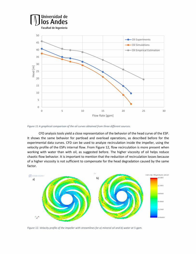
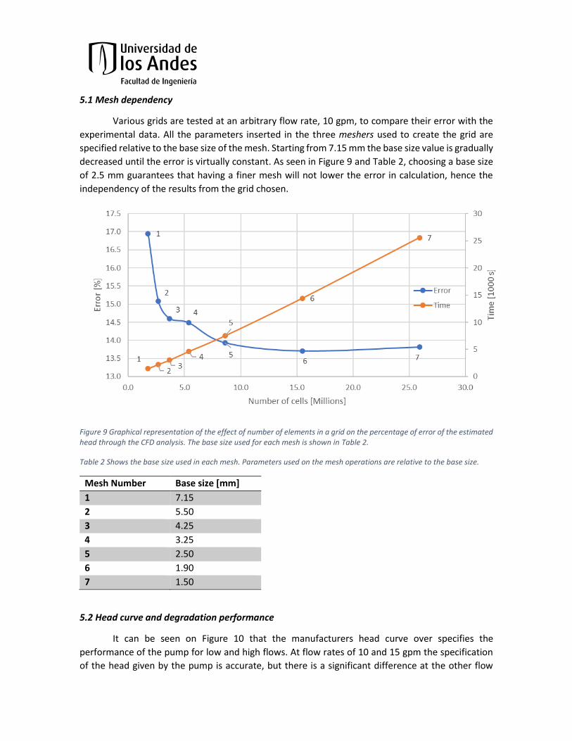
Figure 11 A graphical comparison of the oil curves obtained from three different sources.

CFD analysis tools yield a close representation of the behavior of the head curve of the ESP.

It shows the same behavior for partload and overload operations, as described before for the

experimental data curves. CFD can be used to analyze recirculation inside the impeller, using the

velocity profile of the ESPs internal flow. From Figure 12, flow recirculation is more present when

working with water than with oil, as suggested before. The higher viscosity of oil helps reduce

chaotic flow behavior. It is important to mention that the reduction of recirculation losses because

of a higher viscosity is not sufficient to compensate for the head degradation caused by the same

factor.

Figure 12. Velocity profile of the impeller with streamlines for a) mineral oil and b) water at 5 gpm.

0

5

10

15

20

25

30

35

40

45

50

0 5 10 15 20 25 30

Hea

d [

m]

Flow Rate [gpm]

Oil Experiments

Oil Simulations

Oil Empirical Estimation

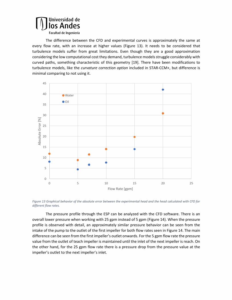
The difference between the CFD and experimental curves is approximately the same at

every flow rate, with an increase at higher values (Figure 13). It needs to be considered that

turbulence models suffer from great limitations. Even though they are a good approximation

considering the low computational cost they demand, turbulence models struggle considerably with

curved paths, something characteristic of this geometry [19]. There have been modifications to

turbulence models, like the curvature correction option included in STAR-CCM+, but difference is

minimal comparing to not using it.

Figure 13 Graphical behavior of the absolute error between the experimental head and the head calculated with CFD for different flow rates.

The pressure profile through the ESP can be analyzed with the CFD software. There is an

overall lower pressure when working with 25 gpm instead of 5 gpm (Figure 14). When the pressure

profile is observed with detail, an approximately similar pressure behavior can be seen from the

intake of the pump to the outlet of the first impeller for both flow rates seen in Figure 14. The main

difference can be seen from the first impeller’s outlet onwards. or the 5 gpm flow rate the pressure

value from the outlet of teach impeller is maintained until the inlet of the next impeller is reach. On

the other hand, for the 25 gpm flow rate there is a pressure drop from the pressure value at the

impeller’s outlet to the next impeller’s inlet.

0

5

10

15

20

25

30

35

40

45

0 5 10 15 20 25

Ab

solu

te E

rro

r [%

]

Flow Rate [gpm]

Water

Oil

Figure 14 Shows the pressure profile through the ESP when working with 25 gpm (a) and 5 gpm (b).

The empirical model under predicts the degradation caused by fluid viscosity. It can be seen

on Figure 11 that the head curve calculated with the empirical method does not show the

“exponentially” increasing pressure losses discussed earlier, the behavior estimates is more that of

a straight line. On the other hand, the overall head curve is a very rough but fairly approximate

estimation. Considering that the empirical approach requires no complex equations to be resolved,

just a few algebraic equations, it is an acceptable method to obtain a first view of the effects of

viscosity on pump performance.

Despite that head degradation calculated with the CFD method does not yield a result

exactly like the experimental values, it is a good approximation when compared to the empirical

method used in this study. Figure 15 shows the difference between the head curve of water and oil

as calculated by each of the three methods in this study. An overall under estimation of head

degradation, leads to an absolute error between 65% and 75% of the head degradation calculated

when comparing the empirical estimation and experimental values from Figure 15 (value at 0 gpm

was not considered). In contrast, absolute error from the CFD method lays between 20% and 40%,

when comparing the simulation and experimental values from Figure 15.

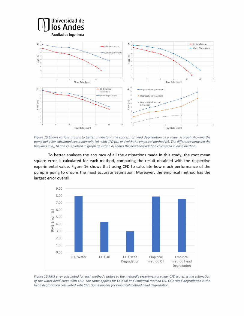
Figure 15 Shows various graphs to better understand the concept of head degradation as a value. A graph showing the pump behavior calculated experimentally (a), with CFD (b), and with the empirical method (c). The difference between the two lines in a), b) and c) is plotted in graph d). Graph d) shows the head degradation calculated in each method.

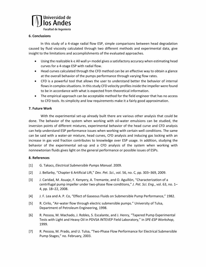
To better analyses the accuracy of all the estimations made in this study, the root mean

square error is calculated for each method, comparing the result obtained with the respective

experimental value. Figure 16 shows that using CFD to calculate how much performance of the

pump is going to drop is the most accurate estimation. Moreover, the empirical method has the

largest error overall.

Figure 16 RMS error calculated for each method relative to the method’s experimental value. CFD water, is the estimation of the water head curve with CFD. The same applies for CFD Oil and Empirical method Oil. CFD Head degradation is the head degradation calculated with CFD. Same applies for Empirical method head degradation.

0,00

1,00

2,00

3,00

4,00

5,00

6,00

7,00

8,00

9,00

CFD Water CFD Oil CFD HeadDegradation

Empiricalmethod Oil

Empiricalmethod HeadDegradation

RM

S Er

ror

[%]

6. Conclusions

In this study of a 4-stage radial flow ESP, simple comparisons between head degradation

caused by fluid viscosity calculated through two different methods and experimental data, give

insight to the limitations and accomplishments of the evaluated approaches.

• Using the realizable k-ε All wall y+ model gives a satisfactory accuracy when estimating head

curves for a 4-stage ESP with radial flow.

• Head curves calculated through the CFD method can be an effective way to obtain a glance

at the overall behavior of the pumps performance through varying flow rates.

• CFD is a powerful tool that allows the user to understand better the behavior of internal

flows in complex situations. In this study CFD velocity profiles inside the impeller were found

to be in accordance with what is expected from theoretical information.

• The empirical approach can be acceptable method for the field engineer that has no access

to CFD tools. Its simplicity and low requirements make it a fairly good approximation.

7. Future Work

With the experimental set-up already built there are various other analysis that could be

done. The behavior of the system when working with oil-water emulsions can be studied, the

inversion points of different mixtures, experimental behavior of the head curve and CFD analysis

can help understand ESP performance issues when working with certain well conditions. The same

can be said with a water-air mixture, head curves, CFD analysis and inducing gas locking with an

increase in gas void fraction contributes to knowledge over ESP usage. In addition, studying the

behavior of the experimental set-up and a CFD analysis of the system when working with

nonnewtonian fluids gives light on the general performance or possible issues of ESPs.

8. References

[1] G. Takacs, Electrical Submersible Pumps Manual. 2009.

[2] J. ellarby, “ hapter 6 Artificial Lift,” Dev. Pet. Sci., vol. 56, no. C, pp. 303–369, 2009.

[3] J. Caridad, M. Asuaje, F. Kenyery, A. Tremante, and O. Aguillón, “ haracterization of a centrifugal pump impeller under two-phase flow conditions,” J. Pet. Sci. Eng., vol. 63, no. 1–4, pp. 18–22, 2008.

[4] J. . Lea and A. P. o, “Effect of Gaseous luids on Submersible Pump Performance,” 1982.

[5] R. irilo, “Air-water flow through electric submersible pumps.” University of Tulsa, Department of Petroleum Engineering, 1998.

[6] R. Pessoa, . achado, J. Robles, S. Escalante, and J. Henry, “Tapered Pump Experimental Tests with Light and Heavy Oil in PDVSA INTEVEP Field Laboratory,” in SPE-ESP Workshop, 1999.

[7] R. Pessoa, . Prado, and U. Tulsa, “Two-Phase Flow Performance for Electrical Submersible Pump Stages,” no. ebruary, 2003.

[8] N. A. V. Bulgarelli, J. L. Biazussi, M. S. de Castro, W. M. Verde, and A. C. Bannwart,

“Experimental Study of Phase Inversion Phenomena in Electrical Submersible Pumps Under Oil Water low,” in ASME 2017 36th International Conference on Ocean, Offshore and Arctic Engineering, 2017, p. V008T11A043-V008T11A043.

[9] D. López, F. Kenyery, . Energy, and U. Simón, “Effect of ubble Size on an ESP Performance Handling Two-Phase low onditions,” Energy Convers., pp. 1–9, 2007.

[10] J. Gamboa and . G. Prado, “ ISUALIZATION STUDY O PER OR AN E REAKDOWN IN TWO-PHASE PERFORMANCE OF AN ELE TRI AL SU ERSI LE PU P by and,” 2009.

[11] R. M. Perissinotto, W. M. Verde, J. L. Biazussi, M. S. De Castro, and A. C. Bannwart, “ isualization of oil droplets within ESP impellers,” Proc. Int. Conf. Offshore Mech. Arct. Eng. - OMAE, vol. 8, pp. 1–8, 2017.

[12] J. L. Turpin, J. . Lea, and J. L. earden, “Gas-Liquid Flow Through Centrifugal Pumps- orrelation of Data,” in Proceedings of the 3rd International Pump Symposium, 1986.

[13] R. Sachdeva, “Two-phase flow through electric submersible pumps.” University of Tulsa, 1988.

[14] R. Sachdeva, D. R. Doty, Z. Schmidt, and U. Tulsa, “Performance of Axial Electric Submersible Pumps in a Gassy Well,” no. 1, 1992.

[15] D. Zhou and R. Sachdeva, “Simple model of electric submersible pump in gassy well,” J. Pet. Sci. Eng., vol. 70, no. 3–4, pp. 204–213, 2010.

[16] . Romero, “An evaluation of an electrical submersible pumping system for high GOR wells.” University of Tulsa, 1999.

[17] J. Zhu, X. Guo, . Liang, and H. Q. Zhang, “Experimental study and mechanistic modeling of pressure surging in electrical submersible pump,” J. Nat. Gas Sci. Eng., vol. 45, pp. 625–636, 2017.

[18] A. J. Stepanoff, Centrifugal and Axial Flow Pumps: Theory, Design, and Application. J. Wiley, 1948.

[19] J. F. Gülich, Centrifugal Pumps. Springer Berlin Heidelberg, 2014.

[20] T. S. ieira, J. R. Siqueira, A. D. ueno, R. E. . orales, and . Estevam, “Analytical study of pressure losses and fluid viscosity effects on pump performance during monophase flow inside an ESP stage,” J. Pet. Sci. Eng., vol. 127, pp. 245–258, 2015.

[21] Hydraulic Institute, Effects of Liquid Viscosity on Rotodynamic (Centrifugal and Vertical) Pump Performance. Parsippany, NJ: Hydraulic Institute, 2004.

[22] KSB, Selecting Centrifugal Pumps. 2005.

[23] S. R. Shah, S. . Jain, R. N. Patel, and . J. Lakhera, “ D for centrifugal pumps: A review of the state-of-the-art,” Procedia Eng., vol. 51, no. NUiCONE 2012, pp. 715–720, 2013.

[24] J. aridad and . Kenyery, “ D Analysis of Electric Submersible Pumps (ESP) Handling Two-

Phase ixtures,” J. Energy Resour. Technol., vol. 126, no. 2, p. 99, 2004.

[25] H. Stel, T. Sirino, P. R. Prohmann, . Ponce, S. hiva, and R. E. . orales, “ D investigation of the effect of viscosity on a three-stage electric submersible pump,” in ASME 2014 4th Joint US-European Fluids Engineering Division Summer Meeting collocated with the ASME 2014 12th International Conference on Nanochannels, Microchannels, and Minichannels, 2014, p. V01BT10A029-V01BT10A029.

[26] H. Pineda et al., “Phase distribution analysis in an Electrical Submersible Pump (ESP) inlet handling water-air two-phase flow using omputational luid Dynamics ( D),” J. Pet. Sci. Eng., vol. 139, pp. 49–61, 2016.

[27] J. Zhu, H. anjar, Z. Xia, and H. Q. Zhang, “ D simulation and experimental study of oil viscosity effect on multi-stage electrical submersible pump (ESP) performance,” J. Pet. Sci. Eng., vol. 146, pp. 735–745, 2016.

[28] E. M. Ofuchi et al., “Numerical investigation of the effect of viscosity in a multistage electric submersible pump,” Eng. Appl. Comput. Fluid Mech., vol. 11, no. 1, pp. 258–272, 2017.

[29] O. abayigit, . Ozgoren, . H. Aksoy, and O. Kocaaslan, “Experimental and D investigation of a multistage centrifugal pump including leakages and balance holes,” Desalin. Water Treat., vol. 67, pp. 28–40, 2017.

[30] Hedland, “ ariable Area low eter EZ-View and Flow-Alert User anual,” p. 24, 2016.

[31] Siemens, “Star + Documentation.” 2018.

[32] H. Stel, T. Sirino, F. J. Ponce, S. Chiva, and R. E. M. Morales, “Numerical investigation of the flow in a multistage electric submersible pump,” J. Pet. Sci. Eng., vol. 136, pp. 41–54, 2015.

[33] Hydraulic Institute, Effects of Liquid Viscosity on Rotodynamic (Centrifugal and Vertical) Pump Performance. Parsippany, NJ: Hydraulic Institute, 2010.