Experimental Evidence on the Economics of Rural Electrification*

Kenneth Lee, Energy Policy Institute at the University of Chicago (EPIC)

Edward Miguel, University of California, Berkeley and NBER

Catherine Wolfram, University of California, Berkeley and NBER

January 2018

ABSTRACT

We present results from an experiment that randomized the expansion of electric grid

infrastructure in rural Kenya. Electricity distribution is a canonical example of a natural

monopoly. Randomized price offers show that demand for electricity connections falls sharply

with price. Experimental variation in the number of connections, combined with administrative

cost data, reveals considerable scale economies, as hypothesized. However, consumer surplus is

far less than total construction costs at all price levels. Moreover, we do not find meaningful

medium-run impacts on economic, health, and educational outcomes, nor evidence of spillovers

to unconnected local households. These results suggest that current efforts to increase residential

electrification in rural Kenya may reduce social welfare. We discuss how leakage of funds,

reduced demand (due to red tape, low reliability, and credit constraints), and other factors may

impact this conclusion.

Acknowledgements: This research was supported by the Berkeley Energy and Climate Institute, the Blum Center for

Developing Economies, the Center for Effective Global Action, the Development Impact Lab (USAID Cooperative

Agreements AID-OAA-A-13-00002 and AIDOAA-A-12-00011, part of the USAID Higher Education Solutions

Network), the International Growth Centre, the U.C. Center for Energy and Environmental Economics, the Weiss

Family Program Fund for Research in Development Economics, the World Bank DIME i2i Fund, and an

anonymous donor. We thank Francis Meyo, Victor Bwire, Susanna Berkouwer, Elisa Cascardi, Corinne Cooper,

Eric Hsu, Radhika Kannan, Anna Kasimatis, Tomas Monárrez, Emma Smith, and Catherine Wright for excellent

research assistance, as well as colleagues at Innovations for Poverty Action Kenya. This research would not have

been possible without the cooperation of partners at the Rural Electrification Authority and Kenya Power. Hunt

Allcott, David Atkin, Severin Borenstein, Raj Chetty, Carson Christiano, Maureen Cropper, Aluma Dembo, Esther

Duflo, Sébastien Houde, Kelsey Jack, Marc Jeuland, Asim Khwaja, Mushfiq Mobarak, Samson Ondiek, Billy Pizer,

Matthew Podolsky, Javier Rosa, Mark Rosenzweig, Manisha Shah, Jay Taneja, Duncan Thomas, Chris Timmins,

Liam Wren-Lewis, and many seminar participants have provided helpful comments. All errors remain our own.

1

I. INTRODUCTION

Investments in infrastructure, including transportation, water and sanitation,

telecommunications, and electricity systems, are primary targets for international development

assistance. In 2015, for example, the World Bank directed a third of its global lending portfolio

to infrastructure.1 The basic economics of these types of investments—which tend to involve

high fixed costs, relatively low marginal costs, and long investment horizons—can justify

government investment, ownership, and subsequent regulation. While development economists

have recently begun to measure the economic impacts of various types of infrastructure,

including transportation (Donaldson 2013; Faber 2014), water and sanitation (Devoto et al. 2012;

Patil et al. 2014), telecommunications (Jensen 2007; Aker 2010), and electricity systems

(Dinkelman 2011; Lipscomb, Mobarak, and Barham 2013; Burlig and Preonas 2016;

Chakravorty, Emerick, and Ravago 2016; Barron and Torero 2017), there remains limited

empirical evidence that links the demand-side and supply-side economics of infrastructure

investments, in part due to methodological challenges. For instance, in many settings it is not

only difficult to identify exogenous sources of variation in the presence of infrastructure, but also

difficult to obtain relevant administrative cost data on infrastructure projects.

In this paper, we analyze the economics of rural electrification. We present experimental

evidence on both the demand-side and supply-side of electrification, specifically, household

connections to the electric grid. We compare demand and cost curves, and evaluate medium-run

impacts on a range of economic, health, and educational outcomes to assess the welfare

implications of mass rural electrification.

The study setting is 150 rural communities in Kenya, a country where grid coverage is

rapidly expanding. In partnership with Kenya’s Rural Electrification Authority (REA), we

provided randomly selected clusters of households with an opportunity to connect to the grid at

subsidized prices. The intervention generated exogenous variation both in the price of a grid

connection, and in the scale of each local construction project. As a result, we can estimate the

demand curve for grid connections among households and, in a methodological innovation of the

current study, the average and marginal cost curves associated with household grid connection

1 In 2014 and 2015, the World Bank allocated nearly 40 percent of total lending towards its Energy and Mining,

Transportation, and Water, Sanitation, and Flood Protection sectors (World Bank Annual Report 2015).

2

projects of varying sizes. We then exploit the exogenous variation in grid connections induced

by the randomized subsidy offers to estimate electrification impacts.

We find that household demand for grid connections is lower than predicted, even at high

subsidy rates. For example, lowering the connection price by 57 percent (relative to the

prevailing price) increases demand by less than 25 percentage points. The cost of supplying

connections, however, is high, even at universal community coverage when the gains from the

economies of scale are attained. As a result, the estimated consumer surplus from grid

connections is far less than the total connection cost at all coverage levels, amounting to less than

one quarter of total costs.

We derive a second measure of the consumer surplus from a grid connection based on the

subsequent benefits derived from consuming electricity, and find it similarly falls far below the

total connection cost. In addition, we do not find economically meaningful or statistically

significant impacts of electrification on a range of economic, health, and educational outcomes in

the medium-run (roughly 18 months post-connection), and no evidence of spillover benefits for

local households.

This constellation of findings points to a perhaps unexpected conclusion, namely, that

investments in rural household electrification may reduce social welfare in our setting. We then

consider the external validity of this finding by presenting and discussing empirical evidence on

the role of excess costs from leakage during construction, and reduced demand due to

bureaucratic red tape, low grid reliability, and credit constraints in our setting.

Electricity systems serve as canonical examples of natural monopolies in

microeconomics textbooks. Empirical estimates in the literature date back to Christensen and

Greene (1976), who examine economies of scale in electricity generation. In recent decades,

initiatives to restructure electricity markets around the world have been motivated by the view

that while economies of scale are limited in generation, the transmission and distribution of

electricity continue to exhibit standard characteristics of natural monopolies (Joskow 2000).

We differentiate between two separate components of electricity distribution. First, there

is an access component, which consists of physically extending and connecting households to the

grid, and is the subject of this paper. Second, there is a service component, which consists of the

ongoing provision of electricity. There is some evidence of economies of scale in both areas.

Engineering studies show how the costs of grid extension may vary depending on settlement

3

patterns (Zvoleff et al. 2009) or can be reduced through the application of spatial electricity

planning models (Parshall et al. 2009). With regards to electricity services, data from municipal

utilities has been used to demonstrate increasing returns to scale in maintenance and billing

(Yatchew 2000). While recent papers have examined the demand for rural electrification using

both survey (Abdullah and Jeanty 2011) and experimental variation (Bernard and Torero 2015;

Barron and Torero 2017), ours is the first study to our knowledge to combine experimental

estimates on the demand for and costs of grid extensions, as well as provide experimental

evidence on later impacts for households. By combining these three elements, we contribute to

ongoing debates regarding the economics of rural electrification in low-income regions.

In Sub-Saharan Africa, roughly 600 million people currently live without electricity (IEA

2014), and achieving universal access to modern energy has become a primary goal for

policymakers, non-governmental organizations, and international donors. In 2013, the U.S.

launched a multi-billion-dollar aid initiative, Power Africa, with a goal of adding 60 million new

connections in Africa. The United Nations Sustainable Development Goals include, “access to

affordable, reliable, sustainable and modern energy for all.” In Kenya, the government has

recently invested heavily in expanding the electric grid to rural areas, and even though the rural

household electrification rate remains low, most households are now “under grid,” or within

connecting distance of a low-voltage line (Lee et al. 2016).2 As a result, the “last-mile” grid

connectivity we study has recently emerged as a political priority in Kenya.

At the macroeconomic level, there is a strong correlation between energy consumption

and economic development, and it is widely agreed that a well-functioning energy sector is

critical for sustained economic growth. There is less evidence, however, on how energy drives

poverty reduction, and how investments in industrial energy access compare to the economic

impacts of electrifying households. For rural communities, there are also active debates about

whether increased energy access should be driven mainly by grid connections or via distributed

solutions, such as solar lanterns and solar home systems (Lee, Miguel, and Wolfram 2016).

Although we find that the estimated consumer surplus from household grid connections is

substantially less than the total connection cost at all coverage levels, universal access to

electricity may still conceivably increase social welfare. For example, mass electrification might

transform rural life in several ways: with electricity, individuals may be exposed to more media

2 In the 2009 Kenya Population and Housing Census, 5.1 percent of rural households use electricity for lighting.

4

and information, might participate more actively in public life and generate improvements in the

political system or public policy, and children could study more and be more likely to obtain

work outside of rural subsistence agriculture later in life. However, roughly 18 months after

gaining an electricity connection, households show little evidence of any such gains, or their

precursors. For instance, there are no meaningful impacts on objective political knowledge

among respondents, nor on child test score performance. Of course, it is possible that the impacts

of electrification take longer to materialize. Long-run impact studies will thus be useful to assess

whether rural electrification should be a development policy priority in African countries.

The remainder of this paper is organized as follows. Section II presents several natural

monopoly scenarios that are empirically tested; Section III discusses rural electrification in

Kenya; Section IV describes the experimental design; Section V presents the main empirical

results; Section VI discusses external validity, focusing on institutional and implementation

challenges to rural electrification, and their implications; and the final section concludes.

II. THEORETICAL FRAMEWORK

In the classic definition, an industry is a natural monopoly if the production of a

particular good or service by a single firm minimizes cost (Viscusi, Vernon, Harrington 2005).

More advanced treatments elaborate on the concept of subadditive costs, which extend the

definition to multiproduct firms (Baumol 1977). Textbook treatments point out that real world

examples involve physical distribution networks, and specifically cite water, telecommunications

and electric power (Samuelson and Nordhaus 1998; Carlton and Perloff 2005; Mankiw 2011).

A. Standard model

We consider the case of an electric utility that provides communities of households with

connections to the grid. To supply these connections, the utility incurs a fixed cost to build a

low-voltage (LV) trunk network of poles and wires in each community. In the standard model,

illustrated in figure 1, panel A, the electricity distribution utility is a natural monopoly facing

high fixed costs, constant or declining marginal costs, and a downward-sloping average total cost

curve. As coverage increases, the marginal cost of connecting an additional household should

decrease, as the distance to the network declines. At high coverage levels, the marginal cost is

essentially the cost of a drop-down service cable that connects a household to the LV network.

5

Household demand for a grid connection reflects expectations about the difference between the

consumer surplus from electricity consumption and the price of monthly electricity service.

The social planner’s solution is to set the connection price equal to the level where the

demand curve intersects the marginal cost curve (p′ in the figure). Due to the natural monopoly

characteristics of the industry, the utility is unable to cover its costs at this price, and the social

planner must subsidize the electric utility to make up the difference. In panel A, total consumer

surplus from the electricity distribution system is positive at price p′ since the area under the

demand curve is greater than the total cost, represented by rectangle with height c′ and width d′.

Note that we are assuming that, once connected, a household can purchase electricity at

the social marginal cost. If this is true, there are no further social gains or losses from electricity

consumption. An alternative approach to estimating the social surplus from a connection is to

calculate the surplus from consuming electricity over the life of the connection. We implement

this approach empirically in Section V.E.3

B. Alternative scenarios and potential externalities from grid connections

We illustrate an alternative scenario in figure 1, panel B. Here, the natural monopolist

faces higher fixed costs. In this case, consumer surplus (the area underneath D) is less than total

cost at all quantities, and a subsidized electrification program reduces social welfare.

In panel C, we maintain the same demand and cost curves as in panel B, but illustrate a

case in which the social demand curve (D′) lies above observed private demand (D). There may

be positive externalities (spillovers) from private grid connections, especially in communities

with strong social ties, where connected households share the benefits of power with neighbors.

In rural Kenya, for instance, people may spend some time in the homes of neighbors who have

electricity, watching TV, charging mobile phones, and enjoying better quality lighting in the

evening. Another factor that could contribute to a gap between D and D′ is the possibility that

households have higher inter-temporal discount rates than policymakers. For example, if

electrification allows children to study more and increases future earnings, there may be a gap if

parents discount their children’s future earnings more than the social planner. Further, observed

private demand may be low due to market failures, such as credit constraints or a lack of

information about the long-run private benefits of a connection; what we are calling the social

demand curve would also reflect the willingness to pay for grid connections if these issues were

3 Appendix A includes a more detailed discussion of the underlying theoretical framework.

6

resolved. In general, if D′ lies above D, there may be a price at which the consumer surplus (the

area underneath D′) exceeds total costs. In the scenario depicted in panel C, D′ is sufficiently

high, and the ideal outcome is to offer full community coverage at price p′′′ and a subsidy equal

to the rectangle with height c′′′ – p′′′ and width d′′′ provided to the utility.

Which of these cases best fits the data? In this paper, we trace out the natural monopoly

cost curves using experimental variation in the connection price and in the scale of each local

construction project. The estimated curves correspond to the segments of figure 1 that range

between the pre-existing rural household electrification rate level, which is roughly 5 percent at

baseline in our data, and full community coverage (d=1). This is the policy relevant range for

governments considering subsidized mass rural connection programs in communities where they

have already installed distribution transformers.

One type of externality that we do not consider is the negative spillover from greater

energy consumption, due to higher CO2 emissions and other forms of environmental pollution.

These would shift the total social cost curve up, making mass electrification less desirable. In the

next section, we discuss aspects of electricity generation in Kenya that make these issues less of

a concern in the study setting than they often are elsewhere.

III. RURAL ELECTRIFICATION IN KENYA

Kenya has a relatively “green” electricity grid, with most energy generated through

hydropower and geothermal plants, and with fossil fuels representing just one third of total

installed electricity generation capacity, which totaled 2,295 megawatts as of 2015. Installed

capacity is projected to increase tenfold by the year 2031, with the proportion of electricity

generated using fossil fuels remaining roughly the same over time.4 Thus Kenya appears poised

to substantially increase rural energy access by relying largely on non-fossil fuel energy sources.

In recent years, there has been a dramatic increase in the coverage of the electric grid. For

instance, in 2003, a mere 285 public secondary schools (3 percent of the total) across the country

had electricity connections, while by November 2012, Kenyan newspapers projected that 100

percent of the country’s 8,436 secondary schools would soon be connected. The driving force

4 Specifically, in 2015, total installed capacity consisted primarily of hydro (36 percent), fossil fuels (35 percent),

and geothermal (26 percent) sources. Based on government planning reports (referred to as Vision 2030), total

installed capacity is expected to reach 21,620 MW by 2031, with fossil fuels (e.g., diesel and natural gas)

representing 32 percent of the total. Many other African countries generate similar shares of electricity from non-

fossil fuel sources (Lee, Miguel, and Wolfram 2016).

7

behind this push was the creation of REA, a government agency established in 2007 to accelerate

the pace of rural electrification. REA’s strategy has been to prioritize the connection of three

major types of rural public facilities, namely, market centers, secondary schools and health

clinics. Under this approach, public facilities not only benefited from electricity but also served

as community connection points, bringing previously off-grid homes and businesses within

relatively close reach of the grid. In June 2014, REA announced that 89 percent of the country’s

23,167 identified public facilities had been electrified. This expansion had come at a substantial

cost to the government, at over $100 million per year. The national household electrification rate,

however, remained relatively low at 32 percent, with far lower rates in rural areas.5 Given this

grid expansion, the Ministry of Energy and Petroleum identified last-mile connections for “under

grid” households as the most promising strategy to reach universal access to power.

During the decade leading up to the study period, any household in Kenya within 600

meters of an electric transformer could apply for an electricity connection at a fixed price of

$398 (35,000 KES).6 The fixed price had initially been set in 2004 and was intended to cover the

cost of building infrastructure in rural areas. As REA expanded grid coverage, the connection

price emerged as a major public issue in 2012, appearing with regular frequency in national

newspapers and policy discussions. The fixed price seemed “too high” for many if not most

poor, rural households to afford. However, Kenya Power, the national electricity utility, held

firm, estimating the cost of supplying a single connection in a grid-covered area to be far higher

at $1,435. After the government rejected its proposal to increase the price to $796 (70,000 KES)

in April 2013, Kenya Power initially announced that it would no longer supply grid connections

in rural areas at all, limiting supply to households that were a single service cable away from an

LV line. As a result, the government agreed to temporarily provide Kenya Power with subsidies

to cover any excess costs incurred, allowing the expansion of rural grid connections to continue

at the same $398 price as before. In February 2014, the government ended these subsidies to

Kenya Power, and it was again widely reported that the price would increase to $796. Ultimately,

the $398 fixed price remained in place for households within 600 meters of a transformer

5 REA provided us with estimates of the proportion of public facilities electrified (June 2014), the national

electrification rate (June 2014), and overall REA investments (between 2012 and June 2015). 6 Baseline and endline Kenya Shilling (KES) amounts are converted into U.S. dollars at the 2014 and 2016 average

exchange rates of 87.94 and 101.53 KES/USD, respectively. The fixed price of 35,000 KES was established in 2004

to reduce the uncertainty surrounding cost-based pricing. Anecdotally, there were concerns that service providers

had earlier lowered the cost-based price in exchange for a bribe.

8

throughout the first phase of our study period, from late-2013 to early-2015, when study

subsidies for electric grid connections were distributed and redeemed.

The government announced in May 2015 (after baseline data collection activities and

redemption of most subsidy offers) that it had secured $364 million—primarily from the African

Development Bank and the World Bank—to launch the Last Mile Connectivity Project (LMCP),

a subsidized mass electrification program that plans to eventually connect four million “under

grid” households, and that, once launched, would lower the fixed connection price to $171

(15,000 KES). This new price was based on the Ministry of Energy and Petroleum’s internal

predictions for take-up in rural areas, and was revealed publicly in May 2015. The take-up data

described in the next section were collected during the decade-long $398 price regime, and

before any public announcement of the planned LMCP program.

IV. EXPERIMENTAL DESIGN AND DATA

A. Sample selection

This field experiment takes place in 150 “transformer communities” in Busia and Siaya,

two counties that are typical of rural Kenya in terms of electrification rates and economic

development and where population density is fairly high (see appendix table B1). Each

transformer community is defined as all households located within 600 meters of a secondary

electricity distribution (low-voltage, LV) transformer, the official distance threshold that Kenya

Power used for connecting buildings at the standard price. The communities were sampled in

cooperation with REA.7

Between September and December 2013, teams of surveyors visited each of the 150

communities to conduct a census of the universe of households within 600 m of the central

transformer. This database, consisting of 12,001 unconnected households in total, served as the

study sampling frame, and showed that 94.5 percent of households remained unconnected

despite being “under grid” (Lee et al. 2016).

Although population density in our setting is fairly high, the average minimum distance

between structures is 52.8 meters.8 These distances make illegal connections quite costly, since

local pole infrastructure would be required to “tap” into nearby lines; in practice, the number of

7 See appendix A for further details and appendix figure B1 for a map of the sample communities.

8 In appendix figure B2, we present a map of a typical (in terms of residential density) transformer community,

illustrating the degree to which unconnected households are within close proximity of an LV line.

9

illegal connections is negligible in the study sample (unlike in some urban areas in Kenya, where

they are anecdotally more common).

For each unconnected household, we calculated the shortest (straight-line) distance to an

LV line, approximated by either the transformer or a connected structure. To limit construction

costs, REA requested that we limit the sampling frame to the 84.9 percent of households located

within 600 meters of a transformer that were also no more than 400 meters away from a low-

voltage line.9 Applying this threshold, we randomly selected 2,289 “under grid” households, or

roughly 15 households per community.

B. Experimental design and implementation

Between February and August 2014, a baseline survey was administered to the 2,289

study households. We additionally collected baseline data for 215 already connected households,

or 30.5 percent of the universe of households observed to be connected to the grid at the time of

the census, sampling up to four connected households in each community, wherever possible.10

In April 2014, we randomly divided the sample of transformer communities into

treatment and control groups of equal size, stratifying the randomization process to ensure

balance across county, market status, and whether the transformer installation was funded early

on (namely, between 2008 and 2010). The 75 treatment communities were then randomly

assigned into one of three subsidy treatment arms of equal size. Following baseline survey

activities in each community, between May and August 2014, each treatment household received

an official letter from REA describing a time-limited opportunity to connect to the grid at a

subsidized price.11

Households were given eight weeks to accept the offer and deposit an amount

equal to the effective connection price (i.e., full price less the subsidy amount) into REA’s bank

account.12

The treatment and control groups are characterized as follows:

1. High subsidy arm: 380 unconnected households in 25 communities are offered a $398

(100 percent) subsidy, resulting in an effective price of $0.

9 In other words, all households located within 400 meters of the transformer were included in the sampling frame,

while some households located between 400 to 600 meters of the transformer were excluded. 10

See appendix A and appendix figure B3 for further details on the experimental design and implementation. 11

An example of this letter is provided in appendix figure B4. 12

Note that in our setting, one does not need a bank account to deposit funds into a specified bank account. The high

subsidy (free treatment) group described below is not subject to the additional ordeal of traveling to town to access a

bank branch, and interacting with bank staff to deposit funds into REA’s account. For those households that do need

to pay something for a connection, the total time and transport cost of such a trip is roughly a few hundred Kenya

Shillings (or a few U.S. dollars), far smaller than the experimental subsidy amounts.

10

2. Medium subsidy arm: 379 unconnected households in 25 communities are offered a $227

(57 percent) subsidy, resulting in an effective price of $171.

3. Low subsidy arm: 380 unconnected households in 25 communities are offered a $114 (29

percent) subsidy, resulting in an effective price of $284.

4. Control group: 1,150 unconnected households in 75 communities receive no subsidy and

face the regular connection price of $398 throughout the study period.

Treatment households also received an opportunity to install a basic, certified household

wiring solution (a “ready-board”) in their homes at no additional cost. Each ready-board—valued

at roughly $34 per unit—featured a single light bulb socket, two power outlets, and two

miniature circuit breakers.13

Each connected household was fitted with a prepaid electricity

meter at no additional charge. At the end of the eight-week period, treatment households could

once again connect to the grid at the standard connection price of $398.

After verifying payments, we provided REA with a list of households to be connected.

This initiated a lengthy process to complete the design, contracting, construction, and metering

of grid connections: the first household was metered in September 2014, the average connection

time was seven months, and the final household was metered over a year later, in October 2015.

Additional details are discussed in Section VI.B below.

Between May and September 2016, we administered an endline survey to 2,217 study

households, or 96.9 percent of the baseline sample. We surveyed an additional 1,345

households—or between six to eleven households per community—as part of a “spillover

sample,” randomly sampling households that were observed to be unconnected at the time of the

census but were not chosen for the baseline survey. Data from this spillover sample is used to

study within-village external impacts. We also collected endline data from 208 of the 215

households that had already been connected at the time of the baseline census. As part of the

endline survey, we additionally administered short English and Math tests to all 12 to 15-year

olds in the endline sample households, or 2,317 children in total.

Following Casey, Glennerster, and Miguel (2012), we registered two pre-analysis plans;

these are available at http://www.socialscienceregistry.org/trials/350 and in appendix C. Pre-

13

The ready-board was designed and produced for the project by Power Technics, an electronic supplies

manufacturer in Nairobi. A diagram of the ready-board is presented in appendix figure B5.

11

Analysis Plan A specifies the analyses of the demand and cost data, and Pre-Analysis Plan B

specifies the analyses of electrification impacts in the endline survey data.

C. Data

The analysis combines a variety of survey, experimental, and administrative data,

collected and compiled between August 2013 and December 2016. The datasets include:

community characteristics data (N=150); baseline household survey data (N=2,504);

experimental demand data (N=2,289); administrative community construction cost data (N=77);

endline household survey data (N=3,770); and children’s test score data (N=2,310).14

D. Baseline characteristics

Table 1 summarizes differences between unconnected and connected households at

baseline. Connected households are characterized by higher living standards across almost all

proxies for income.15

These households have higher quality walls (made of brick, cement, or

stone, rather than the typical mud walls), have higher monthly basic energy expenditures, and

own more land and assets including livestock, household goods (e.g., furniture), and electrical

appliances. Most unconnected households in our sample (92 percent) rely on kerosene as their

primary source of lighting, while only 6 and 3 percent of unconnected households own solar

lanterns and solar home systems, respectively.

In appendix table B2, we report baseline descriptive statistics and perform randomization

checks. On average, 63 percent of respondents are female, just 14 percent have attended

secondary school, 66 percent are married, and, in terms of occupation, 77 percent are primarily

farmers. These are overwhelmingly poor households, as evidenced by the fact that only 15

14

See appendix A for additional details. 15

These patterns are consistent with the stated reasons for why households remain unconnected to electricity. In

appendix figure B6, we show that, at baseline, 95.5 percent of households cited the high connection price as the

primary barrier to connectivity. The second and third most cited reasons—which were the high cost of internal

wiring (10.2 percent) and the high monthly cost (3.6 percent)—are also related to costs. Note that no households

said they were unconnected because they were waiting for a lower connection price, or a government-subsidized

rural electrification program. In fact, prior to our intervention, there were concerns that the price would increase (as

noted above). In appendix figure B7, we present a timeline of project milestones and connection price-related news

reports during the study period. Further, during the intervention, 397 households provided a reason for why they had

declined a subsidized offer and not one cited the possibility of a lower future price. Taken together, these patterns

alleviate concerns that households were anticipating a subsidized government mass electrification program.

12

percent have high-quality walls. Households have 5.3 members on average. Households spend

$5.55 per month on (non-charcoal) energy sources, primarily kerosene.16

We test for balance across treatment arms by regressing household and community

characteristics on indicators for the three subsidy levels, and conduct F-tests that all treatment

coefficients equal to zero. For the 23 household-level and two community-level variables

analyzed, F-statistics are significant at 5 percent for only two variables, namely, a binary

variable indicating whether the respondent could correctly identify the presidents of Tanzania,

Uganda, and the United States (a measure of political awareness) and monthly (non-charcoal)

energy spending, indicating that the randomization created largely comparable groups.

V. RESULTS

A. Estimating the demand for electricity connections

In figure 2, we plot the experimental results on the demand for grid connections. Take-up

of a free grid connection offer is nearly universal, but demand falls sharply with price, and is

close to zero among the low subsidy treatment group, as well as in the control (no subsidy)

group. Panel A presents the experimental results and compares them to the government’s “prior”

on demand, namely, the Ministry of Energy and Petroleum’s internal predictions for take-up in

rural areas. The government demand curve—which we learned of in early-2015 via a

government report—was developed independently of our project and served as justification for

the planned LMCP price of $171 (15,000 KES). A key finding is that, even at generous subsidy

levels, actual take-up is significantly lower than predicted by the government (or by our team,

see appendix figure B8).17

In panels B and C, we show that households with high-quality walls

and greater earnings in the last month, respectively, had higher take-up rates in the medium and

low subsidy arms, suggesting that demand increases at higher incomes.

16

In June 2014, the standard electricity tariff for small households was roughly 2.8 cents per kWh. As a point of

comparison, taking into consideration fixed charges and other adjustments, $5.55 translates into roughly 30 kWh of

electricity consumption, which is enough for basic lighting, television, and fan appliances each day of the month. 17

The government report projected take-up in rural areas nationally, rather than in our study region alone, and this is

one possible source of the discrepancy. Moreover, the government report does not clearly specify the timeframe

over which households would be asked to raise funds for a connection, somewhat complicating the comparison.

13

If we extrapolate the [1.3, 7.1] segment of the demand curve through the intercept, the

area under the demand curve is just $12,421.18

Based on average community density of 84.7

households, this implies an average valuation of just $147 per household.

We estimate the following regression equation:

𝑦𝑖𝑐 = 𝛼 + 𝛽1𝑇𝑐𝐿 + 𝛽2𝑇𝑐

𝑀 + 𝛽3𝑇𝑐𝐻 + 𝑋′𝑐𝛾 + 𝑋′𝑖𝑐𝜆 + 𝜖𝑖𝑐 (1)

where 𝑦𝑖𝑐 is an indicator variable reflecting the take-up decision for household i in transformer

community c. The binary variables 𝑇𝑐𝐿, 𝑇𝑐

𝑀, and 𝑇𝑐𝐻 indicate whether community c was randomly

assigned into the low, medium, or high subsidy arm, respectively, and the coefficients 𝛽1, 𝛽2,

and 𝛽3 capture the subsidy impacts on take-up.19

Following Bruhn and McKenzie (2009), we

include a vector of community-level characteristics, 𝑋𝑐 , containing variables used for

stratification during randomization (see Section IV.B). In addition, we include a vector of

baseline household-level characteristics, 𝑋𝑖𝑐, containing pre-specified covariates that may also

predict take-up (including household size, the number of chickens owned, respondent age, high-

quality walls, and whether the respondent attended secondary school, is not a farmer, uses a bank

account, engages in business or self-employment, and is a senior citizen). Standard errors are

clustered by community, the unit of randomization.

Table 2 summarizes the results of estimating equation 1, where column 1 reports

estimates from a model that includes only the treatment indicators, and column 2 includes the

household and community controls. All three subsidy levels lead to significant increases in take-

up: the 100 percent subsidy increases the likelihood of take-up by roughly 95 percentage points,

and the effects of the partial 57 and 29 percent subsidies are much smaller, at 23 and 6

percentage points, respectively. Columns 3 to 8 include interactions between the treatment

indicators and correlates of household economic status, as well as community variables, which

are listed in the column headings. Take-up in treatment communities is differentially higher in

the low and medium subsidy arms for households with wealthier and more educated respondents;

18

In Section V.C, we discuss alternative assumptions regarding demand in the unobserved [0, 1.3] domain. 19

We focus on this non-parametric specification after rejecting the null hypothesis that the treatment coefficients are

linear in the subsidy amount (F-statistic = 23.03), a choice we specified in our pre-analysis plan.

14

for instance, the coefficient on the interaction between attended secondary school and the

medium subsidy indicator is 19.5 percent.20

Based on the findings in Bernard and Torero (2015), one might expect take-up to be

higher in areas where grid connections are more prevalent if, as they argue, exposure to

households with electricity leads individuals to better understand its benefits and value it more.

Yet when we include an interaction with the baseline community electrification rate in column 6,

or an interaction with the proportion of neighboring households within 200 meters connected to

electricity at baseline (column 7), we find no meaningful interaction effects.21

B. Estimating the economies of scale in electricity grid extension

An immediate consequence of the downward-sloping demand curve estimated above is

that the randomized price offers generate exogenous variation in the proportion of households in

a community that are connected as part of the same local construction project. This novel design

feature allows us to experimentally assess the economies of scale in grid extension. As

hypothesized, we find considerable scale economies. In addition, we find no evidence of

endogeneity as OLS and IV estimates of the effect of scale (e.g., the number of connections) on

the average total cost per connection (“ATC”) are no different.

In the Kenya Power administrative data across all projects in the sample, the actual ATC

is $1,813. While this seems high, it is in line with several alternative estimates, including: (1)

Kenya Power’s public estimate of $1,435 per rural connection; (2) the Ministry of Energy and

Petroleum’s estimate of $1,602; and (3) a consultant’s estimated range of $1,322 to $1,601 in

urban and rural areas, respectively (Korn 2014).22

In figure 3, we plot the fitted curve (light-grey curve) from a regression estimating the

ATC as a quadratic function of community coverage, 𝑄𝑐 (where coverage takes on values from 0

20

In appendix table B3, we compare the characteristics of households choosing to take up electricity across

treatment arms. Households that paid more for an electricity connection (i.e., the low subsidy arm) are wealthier on

average than those who paid nothing (high subsidy), i.e., they are better educated, more likely to have bank

accounts, live in larger households with high-quality walls, spend more on energy, and have more assets. In

appendix tables B4A to B4E, we report all related regressions specified in Pre-Analysis Plan A, for completeness. 21

Of course, this does not rule out the possibility of a differential effect at higher levels of electrification, since

baseline household electrification rates are generally low in our sample of communities (the interquartile range is 1.8

to 7.8 percent). Also, since community-level characteristics, such as income, are likely positively correlated across

households, the lack of statistically significant coefficients may reflect the offsetting joint impacts of negative take-

up spillovers and positively correlated take-up decisions; future research could usefully explore these issues. 22

Elsewhere, rural grid connection costs have been observed to be similar, ranging from $1,100 per connection in

Vietnam to $2,300 per connection in Tanzania (Castellano et al. 2015).

15

to 100).23

The quadratic function does not provide a good fit to the data: it predicts considerably

lower costs at intermediate coverage levels while greatly overstating them at universal

coverage.24

Instead, we focus on an alternative functional form for ATC featuring a community-

wide fixed cost and linear marginal costs:

𝛤𝑐 =𝑏0

𝑄𝑐+ 𝑏1 + 𝑏2𝑄𝑐 (2)

The nonlinear estimation of equation 2 yields coefficient estimates (and standard errors)

of 𝑏0= 2287.8 (s.e. 322.8) for the fixed cost, 𝑏1= 1244.3 (s.e. 159.0), and 𝑏2= -6.1 (s.e. 3.4). We

plot the predicted values from this nonlinear estimation in figure 3 (dark-grey curve).25

We then

take the derivative of the total cost function (which is obtained by multiplying equation 2 by 𝑄𝑐)

to estimate the linear marginal cost function:

𝑀𝐶𝑐 = 𝑏1 + 2𝑏2𝑄𝑐 = $1244.30 − ($12.20)𝑄𝑐 (3)

While this choice of functional form differs from our pre-specified regression model, we

believe that imposing linear marginal costs is both economically intuitive (e.g., as coverage

increases, the marginal cost of connecting an additional household decreases) and closely

matches the observed data. Regardless of the exact functional form, though, average costs

decline in the number of households connected, as in the textbook natural monopoly case.26

While there are strong initial economies of scale, we also document that the incremental cost

savings appear to decline at higher levels of community coverage, and the estimates imply an

average cost of approximately $658 per connection at universal coverage (𝑄𝑐 = 100).

23

Note that in Figure 3, we plot fitted curves by combining two sets of cost data. First, for each community in which

the project delivered an electricity connection (n=62), we received budgeted costs for the number of poles and

service lines, length of LV lines, and design, labor and transportation costs. We refer to these as “sample” data.

Second, REA provided us with budgeted costs for higher levels of coverage (i.e., at 60, 80, and 100 percent of the

community connected) for a subset of the high subsidy arm communities (n=15). We refer to these as “designed”

data. It is important to note that REA followed the same costing methodology for both sets of cost data (e.g., the

same personnel visited the field sites to design the LV network and estimate the costs). This ensured comparability

between budgeted estimates for sample and designed communities. Combining the two sets of cost data (N=77)

enables us to trace out the ATC at all coverage levels. See appendix A for a discussion of the regressions in which

we estimate the impact of either the number of connections or community coverage on the ATC. 24

Despite this poor fit, we include this result because it was specified in our pre-analysis plan. In retrospect, it was

an oversight on our part to fail to include the standard fixed cost at the community level in the model. 25

Appendix table B5A reports actual and predicted ATC values at various coverage levels. 26

In appendix figure B9A, we compare the predicted curve from nonlinear estimation using only sample community

data (N=62) against the predicted curve using both sample and designed community data (N=77). In appendix figure

B9B, we compare alternative functional forms for costs, and the same conclusions hold across cases.

16

In communities with larger populations, the higher density of households may potentially

translate into a larger impact of scale on ATC. In appendix table B5B, column 2, we report the

results of regressions in which we estimate the impact of project scale (i.e., the number of

connections, 𝑀, and a quadratic term, 𝑀2) on ATC, including interactions between community

population and both 𝑀 and 𝑀2. While there are no significant effects in the range of densities

observed in our sample, it seems plausible that per household connection costs could be higher in

other parts of rural Kenya with far lower rates of residential density. There is also no evidence

that higher average land gradient is associated with higher ATC.27

C. Experimental approach to estimating net welfare

In figure 4, we compare the experimental demand curve with the average and marginal

cost curves (panel A), and then estimate total cost and consumer surplus at full coverage (panel

B). We first focus on the revealed preference demand estimates, and discuss issues of credit

constraints and informational asymmetries below in Section VI.B.

The main observation is that the estimated demand curve for an electricity connection

does not intersect the estimated marginal cost curve. To illustrate, at 100 percent coverage, we

estimate the total cost of connecting a community to be $55,713 based on the mean community

density of 84.7 households. In contrast, as noted in Section V.A, consumer surplus at this

coverage level is far less, at only $12,421, or less than one quarter the costs. The consumer

surplus is substantially smaller than total connection costs at all quantity levels, suggesting that

rural household electrification may reduce social welfare. This result is robust to considering the

uncertainty in the demand and cost estimates (see appendix figure B9C).

Specifically, our calculations suggest that a mass electrification program would result in a

welfare loss of $43,292 per community.28

To justify such a program, discounted future social

27

Based on Dinkelman (2011), we expect land gradient to be positively correlated with ATC, but in our setting, the

correlation is, if anything, negative. While the result is counterintuitive, note that there is little variation in average

land gradient in our sample, which ranges from 0.79 to 7.76 degrees. While land gradient may be an important

predictor of the costs of extending high-voltage lines in KwaZulu-Natal, South Africa, as in Dinkelman (2011), our

data suggest that it is less important in predicting construction costs across smaller areas; see appendix figure B10. 28

To calculate consumer surplus, we estimate the area under the unobserved [0, 1.3] domain by projecting the slope

of the demand curve in the range [1.3, 7.1] through the intercept. The 1.3 percent figure is the proportion of the

control group that chose to connect to the grid during the study period, which, for comparability to other points on

the demand curve, we assume would happen over the same eight-week period as our offer. If anything, this

assumption yields higher consumer surplus than alternative, perhaps more reasonable, assumptions on timing.

Appendix figure B11 considers the sensitivity of our results on welfare loss to alternative demand curve

17

welfare gains of $511 would be required for each household in the community, above and

beyond any economic or other benefits already considered by households in their own private

take-up decisions. These welfare gains could take several possible forms, including spillovers in

consumption or broader economic production, an issue we explore below. Credit constraints or

imperfect household information about the long-run benefits of electrification may both also

contribute to lower demand, issues we turn to in the next section, while negative pollution

externalities could raise the social costs of grid connections.

In an alternative scenario, illustrated in appendix figure B12, we estimate the demand for

and costs of a program structured like the LMCP, which planned to offer a connection price of

$171. In this case, only 23.7 percent of households would take-up based on the experimental

estimates, and thus unless the government were willing to provide additional subsidies or

financing, the resulting electrification level would be low. At 23.7 percent coverage, there is an

analogous welfare loss of $22,100 per community, or $1,099 per connected household.

D. Economic impacts of rural electrification

Much of the recent literature on the microeconomics of electrification focuses on

estimating the impacts of increasing access to electricity for rural households and communities.

However, there is substantial variation in the types of outcomes examined, as well as the

magnitudes of impacts estimated.29

Furthermore, non-experimental studies typically face

challenges in identifying credible exogenous sources of variation in electrification status. In

contrast, we exploit experimental variation in grid electrification to test the hypothesis that

households connected to the electricity grid enjoy improved living standards and impacts on

other life outcomes in the medium-run, roughly 18 months post-connection.

We limit our discussion here to a set of ten pre-specified “primary” outcomes that are

meant to capture several important dimensions of overall living standards in the study setting.

The primary outcomes of interest include: household electrification status (denoted outcome P1);

grid electricity spending in the past month (P2); the proportion of household members that are

employed or running their own businesses (P3); total hours worked in the past week (P4); total

assumptions. In panel C of that figure, the most conservative case, demand is a step function and intersects the

vertical axis at $3,000. The welfare loss is still $32,517 per community in this case. 29

For example, some studies find that access to electricity increases measures of rural living standards such as

income and consumption (Khandker, Barnes, and Samad 2012; Khandker et al. 2014; van de Walle et al. 2015;

Chakravorty, Emerick, and Ravago 2016), while others find no evidence of impacts on labor markets outcomes,

assets, or housing characteristics (Burlig and Preonas 2016); see Lee, Miguel and Wolfram (2017) for a review.

18

asset value (P5); annual per capita consumption of major food items (P6); recent health

symptoms (P7); life satisfaction (P8); political and social awareness (P9); and average scores on

an English and Math test administered to adolescent children (P10). Additional details on the

construction of variables are provided in Pre-Analysis Plan B in appendix C.

Due to the relatively low take-up rates in the low and medium subsidy groups, we first

limit the sample to include only a comparison between the high subsidy group and the control

group and estimate intention-to-treat (ITT) specifications. In table 3, column 2, we report the

results of estimating the following regression for each of the 10 primary outcomes:

𝑦𝑖𝑐 = 𝛽0 + 𝛽3𝑇𝐻𝑐 + 𝑋𝑐′𝛬 + 𝑍1𝑖𝑐

′ 𝛤 + 𝜖𝑖𝑐 (4)

where 𝑦𝑖𝑐 represents the primary outcome of interest for household i in community c and 𝑇𝐻𝑐 is a

binary variable indicating whether community c was randomly assigned into the high-value

subsidy treatment. As in equation 1, we include a vector of community-level characteristics, 𝑋𝑐,

as well as a vector of pre-specified, household-level characteristics, 𝑍1𝑖𝑐, and standard errors are

clustered at the community-level.

We then estimate treatment-on-treated (TOT) results using data from all three of the

subsidy treatment groups. In table 3, column 3, we report the results of estimating the following

equation for each of the primary outcomes:

𝑦𝑖𝑐 = 𝛽0 + 𝛽1𝐸𝑖𝑐 + 𝑋𝑐′𝛬2 + 𝑍1𝑖𝑐

′ 𝛤2 + 𝜖𝑖𝑐 (5)

where 𝐸𝑖𝑐, is a binary variable reflecting household i’s electrification status. We instrument for

Eic with the three indicator variables indicating whether community c was randomly assigned to

the low, medium, or high subsidy group.

Column 4 then reports the false discovery rate (FDR)-adjusted q-values corresponding to

the coefficient estimates in column 3, which limit the expected proportion of rejections within a

hypothesis that are Type I errors (i.e., false positives).30

Perhaps surprisingly, but consistent with the results in Section V.B, we do not find

evidence of substantial economic or other impacts stemming from household electrification.

There are no detectable effects on consumption levels, asset ownership, reported health

outcomes, or child test score performance. Although there are small, marginally statistically

30

As per our pre-analysis plan, we follow the FDR approach in Casey et al. (2012) and Anderson (2008).

19

significant impacts on total hours worked (P5) and life satisfaction (P8), these effects do not

survive the FDR multiple testing adjustment. Simply put, we detect few changes in rural Kenyan

households connected to electricity in the medium-run.

These effects are summarized in panel B of table 3, which combines the four primary

economic outcomes (P3-P6) into a mean effect Economic Index, and combines the four primary

non-economic outcomes (P7-P10) into a mean effect Non-Economic Index.31

The average

economic effect is small at 0.03 (in standard deviation units), and reasonably precisely estimated

(s.e. 0.08), and the average effect on the non-economic variables is also small at -0.02 (in

standard deviation units, with s.e. 0.07).

Energy consumption increases in the newly connected households, but overall

consumption levels are quite low. The treatment effect on monthly electricity spending is $2.00

to $2.20, a miniscule amount corresponding to electricity consumption of roughly 3 kWh per

month. The data indicate that treated household acquired few additional appliances, providing an

explanation for the overall lack of positive impacts. For example, in the ITT regression of the

number of appliances owned on the high subsidy indicator, the treatment effect is just 0.2; while

significant at 95 percent confidence, this effect size represents a small increase over the control

mean of 1.8 appliances owned.

Moreover, as shown in appendix table B6, there is no evidence of any meaningful or

statistically significant spillover impacts to local households across the ten primary outcomes.

E. Alternative approach to estimating consumer surplus

Alternatively, we can estimate consumer surplus from grid connections using an

application of Dubin and McFadden’s (1984) discrete-continuous model, similar to Barreca et al.

(2016) and Davis and Killian (2011). This approach then allows us to simulate consumer surplus

for different cases regarding both baseline consumption levels and long-run consumption growth,

under certain functional form assumptions on the consumer demand curve.

Households are assumed to make a joint decision to acquire a grid connection and

consume electricity, and consumer surplus from the connection is then measured as the

discounted sum of surplus from consuming electricity over the life of the connection. We assume

31

Note that these indices were not specified in the pre-analysis. We believe these groupings are still useful in

summarizing related results and providing some additional statistical power in the analysis.

20

zero consumer surplus from electricity without a grid connection.32

Consumer surplus measures

depend on the level of monthly electricity consumption, the demand elasticity for electricity (i.e.,

the slope of the demand curve), the functional form of the demand curve, the long-run cost of

supplying electricity, and the intertemporal discount rate.

This study’s experimental variation in grid connection allows us to measure the shift in

the demand curve for electricity directly based on connected households’ consumption levels.

Lacking demand elasticity estimates in Kenya, we use U.S. estimates as a lower bound (e.g., Ito

2014), and report consumer surplus under a range of plausible assumptions. We assume linear

demand (following Barreca et al. 2016 and Davis and Killian 2011), a price equal to the constant

long-run cost of electricity of $0.12 per kWh, and an annualized 15 percent discount rate.

Table 4 reports calculated consumer surplus across a range of demand elasticity and

consumption cases. In the study sample, the median monthly electricity consumption level for

newly connected households is just 3.6 kWh, an extremely small amount, as noted above. At 5

kWh per month (column 1), consumer surplus ranges from $49 to $147 (depending on demand

assumptions), and thus falls well below the average connection cost in the experiment, which is

in the range of $1,200 to $1,800.33

This result holds even if we assume that energy consumption

grows at a rapid 10 percent per year (see column 2); in this case consumer surplus ranges from

$110 to $329. Column 3 reports estimates at 40 kWh per month, the median consumption level

reported by connected households in our sample at baseline. As further validation of this

approach, consumer surplus at low demand elasticities exceeds $400 (the private cost of a grid

connection). However, it remains below the average connection cost in the experiment.34

In contrast, administrative data from Kenya Power indicates that the median connected

household in Nairobi consumes 72.8 kWh per month.35

At roughly this level of consumption (75

kWh per month, column 4), the rural connections would appear to potentially yield positive

social welfare, with consumer surplus ranging from $733 to $2,200.

32

Note that this will, if anything, lead us to overestimate the consumer surplus from acquiring a grid connection

since a subset of sample households receive electricity from solar home systems or car batteries. 33

Note that consumer surplus at the lowest demand elasticity is the same as the average valuation obtained in the

experiment, even though we arrive at these figures using two distinct methodologies. 34

Furthermore, a full accounting of net welfare for the fraction of households that were initially connected to the

grid should include the costs of the transformer and medium-voltage network extensions. Including these would

greatly increase the overall costs of rural electrification. 35

In appendix table B7, we present various benchmarks for monthly electricity consumption throughout Kenya.

21

VI. EXTERNAL VALIDITY

These results suggesting that rural electrification may reduce social welfare are perhaps

surprising. Previous analyses have found substantial benefits from electrification (Dinkelman

2011, Lipscomb, Mobarak, and Barham 2013), though they have not directly compared benefits

to costs. In the Philippines, Chakravorty, Emerick, and Ravago (2016) find that the physical cost

of grid expansion is recovered after just a single year of realized expenditure gains. A World

Bank report argues that household willingness to pay for electricity—which is calculated

indirectly based on kerosene lighting expenditures—is likely to be well above the average supply

cost in South Asia (World Bank 2008). Most of these studies, however, use non-experimental

variation or indirect measures of costs and benefits, and it is possible they do not fully account

for unobserved variables correlated with both electrification propensity and improved economic

outcomes. In table 1, for example, we document a strong baseline correlation between household

connectivity and living standards, and this pattern is consistent with the possibility of meaningful

omitted variable bias in some non-experimental studies.

In this section, we consider factors that could drive down costs or drive up demand in our

setting, affecting the external validity of our results. Specifically, we present evidence on the role

of excess construction costs from leakage, and reduced demand due to bureaucratic red tape, low

grid reliability, credit constraints, and possibly unaccounted for spillovers.

A. Excess costs from leakage

In appendix table B8, we report the breakdown of budgeted versus invoiced

electrification costs per community. The budgeted (ex-ante) costs for each project are based on

LV network drawings prepared by REA engineers.36

The invoiced (ex-post) costs are based on

actual final invoices submitted by local contractors, detailing the contractor components of the

labor, transport, and materials that were required to complete each project. In total, it cost

$585,999 to build 101.6 kilometers of LV lines to connect 478 households through the project.37

Overall, budgeted and invoiced costs per connection were nearly identical, amounting to

$1,201 and $1,226, respectively. In other words, contractors submitted invoices that were only

36

An example of an LV network drawing is provided in appendix figure B13. 37

See appendix A for additional details.

22

1.7 percent higher than the budgeted amount on average.38

These cost figures reflect the reality

of grid extension in rural Kenya. However, it is possible that they are higher than would ideally

be the case due to leakage and other inefficiencies that are common in low-income countries

(Reinikka and Svenson 2004). In our context, it is possible that leakage occurred during the

contracting work, in the form of over-reporting labor and transport, which may be hard to verify,

and sub-standard construction quality (e.g., using fewer materials than required).39

To measure leakage, we sent teams of enumerators to each treatment community to count

the number of electricity poles that were installed, and then compared the actual number of poles

to the poles included in the project designs and contractor invoices. While there is minimal

variation between ex-ante and ex-post total costs, most contractors’ projects showed large

differences in the number of observed versus budgeted poles with nearly all using fewer poles:

the number of observed poles was 21.3 percent less than budgeted, a substantial discrepancy.40

Labor and transport costs may also reflect leakage. Labor is typically invoiced based on

the number of declared poles, and we showed above that those were inflated. Similarly, transport

is invoiced based on the declared mileage of vehicles carrying construction materials. In

appendix table B9, we analyze three highly detailed contractor invoices (for nine communities)

that were made available to us. These data contain evidence of over-reported labor costs

associated with the electricity poles, at 11.0 percent higher costs than expected, and over-

reported transport costs: based on a comparison between the reported mileage and the travel

routes between the REA warehouse and project sites (suggested by Google Maps), invoiced

travel costs were 32.9 percent higher than expected.

Taken together, these findings indicate that electric grid construction costs may be

substantially inflated due to mismanagement and corruption in Kenya, suggesting that improved

38

The similarity between planned and actual costs provides further confidence that the connection costs for the

designed communities at higher coverage levels (see figure 4) are likely to be reasonably accurate. 39

There is evidence of reallocations across the sub-categories in appendix table B8, despite the similarities between

ex ante and ex post totals. Invoiced labor and transport costs, for example, were 12.7 percent higher in fact than

expected in the plans, while invoiced local network costs were 6.5 percent lower. 40

In appendix figure B14, we plot the discrepancies between costs and poles by contractor. In addition to being

associated with missing public resources, if the planned number of poles reflects accepted engineering standards

(i.e., poles are roughly 50 meters apart, etc.), using fewer poles might lead to substandard service quality and even

safety risks. For instance, local households may face greater injury risk due to sagging power lines between poles

that are spaced too far apart, and the poles may be at greater risk of falling over. It is possible, however, that REA’s

designs included extra poles, perhaps anticipating that contractors would not use them all.

23

contractor performance could reduce costs and possibly improve project quality and safety.41

On

the other hand, note that even with a 20 to 30 percent reduction in construction costs, mass rural

household electrification would still lead to a reduction in overall social welfare based on the

demand and cost estimates in figure 4, as well as the consumer surplus results in table 4 below.

B. Factors contributing to lower demand for electricity connections

We next discuss several factors that potentially contribute to lower levels of observed

household demand for electricity connections, including bureaucratic red tape, low grid

reliability, credit constraints, and unaccounted for positive spillovers.

Low levels of demand may be partly attributable to the lengthy and bureaucratic process

of obtaining an electricity connection. In our sample, households waited a staggering 188 days

after submitting their paperwork before they began receiving electricity. The delays were mainly

caused by time lags in project design and contracting, as well as in the installation of meters.42

The World Bank similarly estimates that in practice it takes roughly 110 days to connect new

business customers in Kenya (World Bank 2016).

Another major concern is the reliability of power. Electricity shortages and other forms of

low grid reliability are well documented in less developed countries (Steinbuks and Foster 2010;

Allcott, Collard-Wexler, and O’Connell 2016). In rural Kenya, households experience both

short-term blackouts, which last for a few minutes up to several hours, and long-term blackouts,

which can last for months and typically stem from technical problems with local transformers.

The value a household places on an electric grid connection could be substantially lower when

service is this unreliable.

During the 14-month period from September 2014 to October 2015 when households

were being connected to the grid, we documented the frequency, duration, and primary reason

for the long-term blackouts impacting sample communities. In total, 29 out of 150 transformers

(19 percent) experienced at least one long-term blackout. On average, these blackouts lasted four

months, with the longest lasting an entire year. During these periods, households and businesses

did not receive any grid electricity. The most common reasons included transformer burnouts,

41

To the extent costs are high because contractors are over-billing the government, leakage may simply result in a

transfer across Kenyan citizens and not a social welfare loss. The social welfare implications would depend on the

relative weight the social planner places on contractors, taxpayers, and rural households. 42

Field enumerators report that the electricity connection work may have sometimes been delayed due to

expectations that bribes would be paid. See appendix A for additional details.

24

technical failures, theft, and replaced equipment.43

As a point of comparison, only 0.2 percent of

transformers in California fail over a five year period, with the average blackout lasting a mere

five hours.44

That said, there is no strong statistical evidence that recent blackouts affect demand:

column 8 in table 2 includes interactions between the treatment variables and an indicator for

whether any household in the community reported a recent blackout (over the past three days) at

baseline, but finds no statistically significant effects.

Low demand may also be driven in part by household credit constraints, which are well

documented in developing countries (De Mel, McKenzie, and Woodruff 2009; Karlan et al.

2014). In our context, concerns about the role of credit constraints may be exacerbated by the

fact that we study a short-run subsidy offer for an electricity connection, redeemable over eight

weeks, rather than a permanent change in the connection price across villages (which would

provide households with more time to raise the necessary funds); long-term differential prices

across villages were not politically feasible in the study setting.

In figure 5, we compare the experimental results to two sets of stated willingness to pay

(WTP) results obtained in the baseline survey to shed some light on this issue. Stated WTP may

better capture household valuation in the presence of credit constraints, although this is

debatable, since they may also systematically overstate actual demand due to wishful thinking or

social desirability bias (Hausman 2012).

Respondents were first asked whether they would accept a randomly assigned,

hypothetical price ranging from $0 to $853 for a grid connection.45

Households were then asked

whether they would accept the hypothetical offer if required to complete the payment in six

weeks, a period chosen to be similar to the eight-week payment period in the experiment. We

plot results in figure 5, where the first curve (long-dashed line, black squares) plots the results of

the initial question, and the second curve (long-dashed line, grey squares) the follow-up question.

Stated demand is generally high.46

However, the demand curve falls dramatically when

households are faced with a hypothetical time constraint, suggesting they are unable to pay (or

43

In appendix table B10, we provide a list of all the communities that experienced long-term blackouts. 44

Based on personal communications with Pacific Gas and Electric Company (PG&E) in December 2015. 45

Each of $114, $171, $227, $284, and $398 had a 16.7 percent chance of being drawn. Each of $0 and $853 had an

8.3 percent chance of being drawn. Nine households are excluded due to errors in administering the question. 46

For more details on the stated demand for electricity connections, see appendix table B11A, where we estimate

the impact of the randomized offers on hypothetical and actual take-up, and appendix table B11B, which includes

interactions between indicators for the hypothetical offers and key household covariates. In appendix figure B15, we

plot hypothetical demand curves for households with and without bank accounts and high-quality walls.

25

borrow) the required funds on relatively short notice, an indication that credit constraints may be

binding. An alternative interpretation is that the hypothetical question without time constraints

generates exaggerated demand figures. At a price of $171, for example, stated demand is initially

57.6 percent but it drops to 27.2 percent with the time constraint.

Although the experimental demand curve is substantially lower than the stated demand

without time limits, it more closely tracks the constrained stated demand: at $171, actual take-up

in the experiment is 23.7 percent. The difference between the two contingent valuation results is

consistent with the evidence on hypothetical bias (Murphy et al. 2005; Hausman 2012).

However, the similarity between the constrained stated demand and experimental results suggest

that augmenting survey questions to incorporate realistic timeframes and other contextual factors

could help to elicit responses that more closely resemble revealed preference behavior.

We also regressed a binary variable indicating whether a household first accepted the

hypothetical offer without the time constraint, but then declined the offer with the time constraint

on a set of household covariates. Households with low-quality walls and respondents with no

bank accounts are the most likely to switch their stated demand decision when faced with a

pressing time constraint, consistent with the likely importance of credit constraints for these

groups (see appendix table B11C).

In Section V.C above, we combined the experimental demand and cost curves and show

that rural electrification may reduce social welfare. The stated preference results indicate that this

outcome is likely to hold even if credit constraints were eased. For example, if we combine the

cost curve with the stated demand for grid connections without time constraints, then households

in the unobserved [0, 16.7] domain of the stated demand curve (i.e., those willing to pay at least

$853) must be willing to pay $2,920 on average for consumer surplus to be larger than total

construction costs. While this cannot be ruled out, it appears unlikely in a rural setting where

annual per capita income is below $1,000 for most households.47

Furthermore, the ITT results in table 3, column 2 imply that medium-run impacts of

electrification on economic (and other) outcomes are close to zero even when credit constraints

are eliminated—by the high subsidy offer, which pushed the connection price to zero—providing

further evidence that consumer surplus from grid connections is likely to be relatively low.

47

The area under the stated demand curve (without time constraints) is roughly $447 per household, under the

assumption that the demand curve can be extended linearly in the [0, 16.7] range, intersecting the y-axis at $2,158.

26

Another way to address credit constraints is to offer financing plans for grid connections.

In a second set of baseline stated WTP questions, each household was randomly assigned a

hypothetical credit offer consisting of an upfront payment (ranging from $39.80 to $127.93), a

monthly payment (from $11.84 to $17.22), and a contract length (either 24 or 36 months); we

present the results in figure 5.48

Households were first asked whether they would accept the offer

(short-dashed line, black circles) and then whether they would accept the offer if required to

complete the upfront payment in six weeks (grey circles). We then plot take-up against the net

present value of the credit offers based on an annualized 15 percent discount rate.

When households are offered financing, stated demand is not only high but also appears

likely to be exaggerated, particularly when there are no time constraints to complete the upfront

payments. For example, 52.7 percent of households stated that they would accept the $915.48 net

present value offer, a package that consists of an upfront payment of $127.93 and monthly

payments of $26.94 for 36 months. Eight weeks after accepting such an offer, a borrower will

have paid $181, with an additional $915.92 due in the future. Yet stated demand for this option is

twice as high as what we observe for the actual $171 time-limited, all-in price offered to medium

subsidy arm households in the experiment. Moreover, the fact that stated take-up is very similar

across hypothetical contract offers with quite divergent net present values casts some doubt on

the reliability of these stated preference responses. The area under the stated demand curve in the

case with financing and without time constraints is roughly $744 per household (under the same

assumptions as above), which again falls short of average costs in our setting.

Figure 5 combines the four stated demand curves with the experimental demand and

ATC curves. Visually, the only demand curves that appear to yield consumer surpluses that are

potentially larger than total construction costs are the stated demand curves for grid connections

with credit offers, which as we point out above, could be overstated.

Finally, low demand may indicate that even with subsidies, grid connections are simply

too expensive for many of the households in our poor rural setting. After the experiment, we

asked households that were connected in the low and medium subsidy arms to name any

sacrifices they had made to complete their payments: 29 percent of households stated that they

had forgone purchases of basic household consumption goods, and 19 percent stated that they

48

Results for a range of discount rates and net present values are presented in appendix table B12.

27

had not paid school fees. It seems likely that many households declined the subsidized offer due

to binding budget constraints, in other words, poverty, rather than credit constraints alone.

C. Is rural electrification a socially desirable policy?

The leading interpretation of our empirical findings is that mass rural household

electrification does not improve social welfare in Kenya, according to standard criteria. The cost

of electrifying households appears to be at least four times higher than what households are

willing and able to pay for these connections, and consumer surplus appears lower than total

costs even with demand estimates that attempt to address credit constraints, or utilize subsequent

electricity consumption patterns among connected households. While per household costs fall

sharply with coverage, reflecting the economies of scale in the creation of local grid

infrastructure, they remain far higher than demand, implying that social welfare falls with each

additional subsidized connection. These results are also consistent with the evidence of

negligible medium-run economic, health and educational impacts 18 months post-connection.

Yet, it is possible that these conclusions would change in settings with improved

organizational performance by the electricity utility, or different levels of economic

development. In table 5, we simulate the cost, consumer surplus, and net welfare per household

using both the experimental approach presented in Section V.C and the alternative demand

approach in Section V.E., under a range of assumptions about the underlying institutional and

economic setting. In particular, we simulate the impact of “improving” the setting in five distinct

ways: (a) allowing for household income growth of 3 percent per annum over 30 years (for the

experimental approach) and electricity consumption growth of 10 percent per annum over 30

years (for the alternative approach); (b) alleviating credit constraints for grid connections; (c)

eliminating transformer breakdowns; (d) eliminating the grid connection delays households face;

and (e) eliminating all project construction cost leakage.49

We examine these individually, and

then assess the effect on consumer surplus of combining them all in what we call the “ideal

scenario”, which can be thought of as perhaps the best-case scenario for a low-income country

considering mass rural residential electrification.

The first row of table 5 presents the base results from the above analysis, including the

average connection cost (at 100 percent coverage) of $658, average consumer surplus from the

49

In appendix table B13, we present an additional adjustment accounting for the consumer surplus associated with

households that were already connected at baseline, and note that this adjustment does not change our conclusions.

28

experimental approach of $147, and from the alternative approach of $147. As Kenya continues

to develop, it is reasonable to assume that incomes and energy consumption will grow. To

predict the effect of income growth on consumer surplus, we focus on the relative differences

between households with low- and high-quality walls. For instance, the difference in

experimental demand curves between these groups (figure 2, panel B) translates into a 2.2

percent annual growth rate of consumer surplus over ten years. Similarly, we estimate that the

income difference between households with low- and high-quality walls translates into a 3

percent annual growth rate of income over ten years.50

Extrapolating these relationships over a

30-year period, consumer surplus per household reaches $285, thus increasing by $139 (row a).

We further refine the estimates of consumer surplus in the experimental approach by

relaxing credit constraints, using the valuations from the stated WTP question without time

constraints described above (row b).51

This more than triples consumer surplus, but is not enough

to alter the conclusion that net welfare is likely to be negative. Similarly, while rapid electricity

consumption growth in the coming 30 years (at 10 percent per year) leads to a large increase in

consumer surplus in the alternative approach, it is not enough to offset the upfront cost (row a).

We next turn to simulated improvements in service provision that address transformer

breakdowns (row c) and grid connection delays (row d), both of which somewhat increase

consumer surplus, in the first case by increasing the number of days of service, and in the second

case by assuming consumers get access to power sooner. As a rough approximation, we assume

demand estimates scale linearly. Neither improvement on its own is sufficiently large enough to

overturn the negative net welfare conclusion.

Finally, we simulate a reduction in total construction costs of 21.3 percent consistent with

the degree of over-invoicing of construction poles documented in the data (row e). This leads to

a sharp reduction in total costs under the assumption that this leakage is simply “waste”; leakage

would far be less socially costly if viewed simply as a transfer from taxpayers to contractors

(though would still incur some deadweight loss associated with the cost of raising funds).

50

As a proxy for the difference in income, we use food consumption per capita at endline. Note that we did not have

a comprehensive measure of household income or consumption at baseline. Our baseline measure of monthly

earnings—calculated as the sum of the respondent’s profits from businesses and self-employment; salary and

benefits from employment; and agricultural sales for the household—is imperfect as it excludes earnings from other

household members as well as subsistence agriculture. 51

Note that the alternative approach reflects consumer surplus from a grid connection largely absent credit

constraints since it presumes that the household already has a connection.

29

The bottom row presents the ideal scenario in which all improvements are simultaneously

implemented. The use of the preferred experimental estimates incorporating the easing of credit

constraints and future income growth results in a net welfare gain of $148. The alternative

estimates using electricity consumption (and assuming rapid future consumption growth) are

more negative, with a net welfare loss of $144. The bottom line is that, even under optimistic

assumptions about the reduction of corruption and improvements in electricity service quality,

together with sustained economic growth, mass rural residential electrification may or may not

be an attractive public investment, and even if it is, the magnitude of any gains may not be large.

There may also be additional benefits that are not captured by household WTP that could

make this calculation appear more positive. First, as outlined in Section II.B, there may be

spillovers from private grid connections, including any benefits that local unconnected

households experience. Yet as mentioned in Section V.A above, we find no evidence of an

interaction between the treatment indicators and the local baseline electrification rate.52

More

importantly, there is no evidence of spillover impacts for local unconnected households along a

range of economic, health and educational outcomes using endline survey data, as noted above.

Second, grid connections are long-lived but their long-term benefits may not be fully

reflected in WTP if households have limited information about the future income or broader

welfare benefits of electrification, or due to imperfect within-household altruism, for instance, if

children stand to gain the most from indoor lighting in the evening (if it boosts learnings and

future earning) but their parents do not fully understand these gains or incorporate them into

decision-making. However, as noted above we do not find evidence for child test score gains in

connected households in the medium-run.

Further, other factors may push up costs, making rural electrification less attractive. The

per household connection cost would be substantially higher under a policy in which only a

subset of households were connected to the grid (given the fixed costs of expanding the local low

voltage network), rather than the mass connection case we assume in Table 5. Most importantly,

access to modern energy could generate negative environmental externalities from higher CO2

emissions and other forms of pollution.

52

Note that we cannot rule out the possibility that any negative effect of these spillovers on take-up due to free-

riding is offset by a competing positive “keeping up with the neighbors” mechanism (Bernard and Torero 2015), or

that greater learning about the private benefits of electricity and/or correlated household characteristics are present.

30

Moreover, we have considered neither the costs nor economic benefits of the initial

investment to extend the high-voltage lines and install transformers in each sample community.

Each installation required a large investment—the median cost per transformer is $21,820 (Lee

et al. 2016)—and the welfare gains from powering the targeted public facilities, while potentially

large, have not been measured. Our analysis treats these costs as sunk and focuses solely on the

economics of electrifying “under grid” households, conditional on existing infrastructure. This is

the policy-relevant question in our setting, given the expanding Kenya LMCP, but the cost of

transformer installations would need to be considered in many other African and Asian settings.

VII. CONCLUSION

Over the past century, rural electrification has served as a key benchmark for economic

development and social progress. The United States began its mass rural electrification program

in the late-1930s, though it required two decades to reach 90 percent of households (Kitchens

and Fishback 2015), China did so in the 1950’s, and South Africa launched its initiative in the

1990s. Today, access to energy has emerged as a major political issue in many low-income

countries, as they aim to repeat the successes of earlier mass electrification programs.

However, the extent to which increases in energy access should be driven by investments

in large-scale infrastructure, such as grid connections, or small-scale decentralized solutions,

such as solar lanterns and solar home systems, remains contested. Does Africa’s energy future

even lie with the grid? Although our findings suggest that household electrification may reduce

social welfare, they do not necessarily imply that distributed solar systems are any more

attractive than the grid, or that the patterns we identify are universal across time and space. In

fact, the evidence—on inflated construction costs from leakage, and the pervasiveness of

bureaucratic red tape, low grid reliability, and household credit constraints, all of which would

suppress demand—suggests that the social welfare consequences of rural electrification are

closely tied to organizational performance as well as institutions. We show that settings with

better performance by the electricity utility—with fewer losses due to leakage and service that is

more responsive to customers—may see shifts in both the cost curve and the demand side, and in

such settings mass rural electrification may potentially be the socially optimal policy.

Another possibility is that mass electrification is indeed transformative and reshapes

social, political, and economic interactions, perhaps in the long-run, but individual rural

31

households do not internalize these benefits, and they are neither reflected in private demand

estimates nor observable in the medium-run follow-up data collected 18 months post-connection.

Rural Kenyan households today may on average be too poor to consume meaningful amounts of

electricity, but perhaps after another decade (or two) of sustained income growth they will be

able to purchase the complementary appliances needed to fully exploit electrification’s promise.

Decisions to invest in large-scale energy infrastructure programs are associated with

major opportunity costs and long-run consequences for future economic development and

climate change, especially in Sub-Saharan Africa, where access to electricity lags the rest of the

world. The findings of this study indicate that connecting rural households today is not

necessarily an economically productive and high return activity in the world’s poorest countries.

The social returns to investments in transportation, education, health, water, sanitation, or other

sectors—indeed possibly including the electrification of industrial sites or urban areas—need to

be compared to investments in rural electricity grid expansion to determine the appropriate

sequencing of major public investments. Given the high stakes around these decisions, and the

limited evidence base, there is a need for research in several areas, including generating further

evidence on the impacts of increasing the supply of electricity, both in terms of access and

reliability, to different types of consumers, such as commercial and industrial consumers;

identifying the patterns and drivers of consumption demand, including for energy-efficient

appliances; and determining routes to improving electric utility organizational performance.

REFERENCES

Abdullah, Sabah, P. Wilner Jeanty. 2011. “Willingness to Pay for Renewable Energy: Evidence

from a Contingent Valuation Survey in Kenya." Renewable and Sustainable Energy Reviews

15(6): 2974-2983

Allcott, Hunt, Allan Collard-Wexler, Stephen D. O'Connell. 2016. “How Do Electricity

Shortages Affect Industry? Evidence from India.” American Economic Review 106(3): 587-624.

Aker, Jenny C. 2010. “Information from Markets Near and Far: Mobile Phones and Agricultural

Markets in Niger.” American Economic Journal: Applied Economics 2: 46-59.

Anderson, Michael L. 2008. “Multiple Inference and Gender Differences in the Effects of Early

Intervention: A Reevaluation of the Abecedaian, Perry Preschool, and Early Training Projects.”

Journal of the American Statistical Association 103(484): 1481-1495.

Barreca, Alan, Karen Clay, Olivier Deschenes, Michael Greenstone and Joseph Shapiro. 2016.

“Adapting to Climate Change: The Remarkable Decline in the US Temperature-Mortality

Relationship over the Twentieth Century.” Journal of Political Economy 124(1): 105-159.

32

Baumol, William J. 1977. “On the Proper Cost Tests for Natural Monopoly in a Multiproduct

Industry." American Economic Review 67(5): 809-822.

Barron, Manuel, Maximo Torero. 2017. “Household Electrification and Indoor Air Pollution.”

Journal of Environmental Economics and Management 86: 81-92.

Bernard, Tanguy, Maximo Torero. 2015. “Social Interaction Effects and Connection to

Electricity: Experimental Evidence from Rural Ethiopia.” Economic Development and Cultural

Exchange 63(3): 459-484.

Bruhn, Miriam, David McKenzie. 2009. “In Pursuit of Balance: Randomization in Practice in

Development Field Experiments.” American Econ. Journal: Applied Economics 1(4): 200-232.

Burlig, Fiona and Louis Preonas. 2016. “Out of the Darkness and Into the Light? Development

Effects of Electrification in India”, unpublished manuscript.

Carlton, Dennis W., Jeffrey M. Perloff. 2005. Modern Industrial Organization. Boston:

Pearson/Addison Wesley.

Casey, Katherine, Rachel Glennerster, Edward Miguel. 2012. “Reshaping Institutions: Evidence

on Aid Impacts Using a Preanalysis Plan.” Quarterly Journal of Economics 127(4): 1755-1812.

Castellano, Antonio, Adam Kendall, Mikhail Nikomarov, and Tarryn Swemmer. 2015. Brighter

Africa: The growth potential of the sub-Saharan electricity sector. McKinsey, available at

http://www.mckinsey.com.

Chakravorty, Ujjayant, Kyle Emerick, Majah-Leah Ravago. 2016. “Lighting Up the Last Mile:

The Benefits and Costs of Extending Electricity to the Rural Poor”, unpublished manuscript.

Christensen, Laurits R., and William H. Greene. 1976. “Economies of Scale in U.S. Electric

Power Generation.” Journal of Political Economy 84(4): 655-676.

Davis, Lucas and Lutz Killian. 2011. “The Allocative Cost of Price Ceilings in the U.S.

Residential Market for Natural Gas.” Journal of Political Economy 119 (2): 212-241.

de Mel, Suresh, David McKenzie, Christopher Woodruff. 2009. “Are Women More Credit

Constrained? Experimental Evidence on Gender and Microenterprise Returns.” American

Economic Journal: Applied Economics 1(3): 1-32.

Devoto, Florencia, et al. 2012. “Happiness on Tap: Piped Water Adoption in Urban Morocco.”

American Economic Journal: Economic Policy 4(4): 68-99.

Dinkelman, Taryn. 2011. “The Effects of Rural Electrification on Employment: New Evidence

from South Africa.” American Economic Review 101(7): 3078–3108.

Donaldson, Dave. 2013. “Railroads of the Raj: Estimating the Impact of Transportation

Infrastructure.” American Economic Review, forthcoming.

Faber, Benjamin. 2014. “Trade Integration, Market Size, and Industrialization: Evidence from

China’s National Trunk Highway System.” Review of Economic Studies 81(3): 1046-1070.

Korn, Andreas. 2014. “Consultancy Services for Development of Electricity Connection Policy

and Draft Regulations.” Fichtner Management Consulting.

33

Hausman, Jerry. 2012. “Contingent Valuation: From Dubious to Hopeless.” Journal of Economic

Perspectives 26(4): 43-56.

Kitchens, Carl, and Price Fishback. 2015. “Flip the Switch: The Impact of the Rural

Electrification Administration 1935-1940.” Journal of Economic History 75(4): 1161-1195.

IEA (International Energy Agency). 2014. Africa Energy Outlook.

Ito, Koichiro. 2014. “Do Consumers Respond to Marginal or Average Price? Evidence from

Nonlinear Electricity Pricing.” American Economic Review 104(2): 537-563.

Jensen, Robert. 2007. “The Digital Provide: Information (Technology), Market Performance, and

Welfare in the South Indian Fisheries Sector.” Quarterly Journal of Economics 122(3): 879-924.

Joskow, Paul. 2000. “Deregulation and Regulatory Reform in the U.S. Electric Power Sector,” in

Deregulation of Network Industries: What’s Next? Sam Peltzman and Clifford Winston, eds.

Washington, D.C.: AEI-Brookings Joint Center for Regulatory Studies, pp. 113-54.

Karlan, Dean, Robert Osei, Isaac Osei-Akoto, Christopher Udry. 2014. “Agricultural Decisions

After Relaxing Credit and Risk Constraints.” Quarterly Journal of Economics 129(2): 597-652.

Khandker, Shahidur R., Douglas F. Barnes, and Hussain A. Samad. 2012. “The Welfare Impacts

of Rural Electrification in Bangladesh.” Energy Journal 33(1): 187-206.

Khandker, Shahidur R., Hussain A. Samad, Rubaba Ali, and Douglas F. Barnes. 2014. “Who

Benefits Most from Rural Electrification? Evidence in India.” Energy Journal 35(2): 75-96.

Lipscomb, Molly, Mobarak, Ahmed Mushfiq, Tania Barham. 2013. “Development Effects of

Electrification: Evidence from the Topographic Placement of Hydropower Plants in Brazil.”

American Economic Journal: Applied Economics 5(2): 200-231.

Lee, Kenneth, Eric Brewer, Carson Christiano, Francis Meyo, Edward Miguel, Matthew

Podolsky, Javier Rosa, Catherine Wolfram. 2016. “Electrification for “Under Grid” Households

in Rural Kenya.” Development Engineering 1: 26-35.

Lee, Kenneth, Edward Miguel, Catherine Wolfram. 2016. “Appliance Ownership and

Aspirations among Electric Grid and Home Solar Households in Rural Kenya.” American

Economic Review: Papers & Proceedings 106(5): 89-94.

Lee, Kenneth, Edward Miguel, Catherine Wolfram. 2017. “Electrification and Economic

Development: A Microeconomic Perspective.” EEG State-of-Knowledge Paper Series.

Mankiw, N. Gregory. 2011. Principles of Economics, 5th Edition. Cengage Learning.

Murphy, James J., et al. 2005. “A Meta-Analysis of Hypothetical Bias in Stated Preference

Valuation.” Environmental and Resource Economics 30(3): 313-325.

Samuelson, Paul A., and William D. Nordhaus. 1998. Economics. Boston: Irwin/McGraw-Hill.

Parshall, Lily, et al.. 2009. “National Electricity Planning in Settings with Low Pre-Existing Grid

Coverage: Development of a Spatial Model and Case Study of Kenya.” Energy Policy 37(6):

2395-2410.

34

Patil, Sumeet R., et al. 2014. “The Effect of India’s Total Sanitation Campaign on Defecation

Behaviors and Child Health in Rural Madhya Pradesh: A Cluster Randomized Controlled Trial”

PLoS Medicine 11(8): e1001709.

Reinikka, Ritva, Jakob Svensson. 2004. “Local Capture: Evidence from a Central Government

Transfer Program in Uganda.” Quarterly Journal of Economics 119(2): 679-705.

Steinbuks, J., and V. Foster. 2010. “When Do Firms Generate? Evidence on In-House Electricity

Supply in Africa.” Energy Economics 32(3): 505-14.

van de Walle, Dominique, Martin Ravallion, Vibhuti Mendiratta, and Gayatri Koolwal. 2015.

“Long-Term Gains from Electrification in Rural India.” World Bank Economic Review: 1-36.

Viscusi, W. Kip, John M. Vernon, and Joseph Emmett Harrington. 2005. Economics of

Regulation and Antitrust. Cambridge, Mass: MIT Press.

World Bank. 2008. “The Welfare Impact of Rural Electrification: A Reassessment of the Costs

and Benefits. An IEG Impact Evaluation.” Washington, DC.

World Bank. 2016. “Doing Business 2016: Measuring Regulatory Quality and Efficiency.”

Washington, DC.

Yatchew, Adonis. 2000. “Scale Economies in Electricity Distribution: A Semiparametric

Analysis.” Journal of Applied Econometrics 15: 187-210.

Zvoleff, Alex, Ayse Selin Kocaman, Woonghee Tim Huh, and Vijay Modi. 2009. “The Impact

of Geography on Energy Infrastructure Costs.” Energy Policy 37 (10): 4066-4078.

Figure 1—The electric utility as a natural monopoly

Panel A Panel B Panel C

Notes: In panel A, the electric utility is a natural monopoly facing high fixed costs, decreasing marginal costs (MCA), and decreasing average totalcosts (ATCA). MCA intersects demand at d′. At d′, a government-subsidized mass electrification program would increase social welfare sinceconsumer surplus (i.e., the area under the demand curve) is greater than total cost. Panel B illustrates an alternative scenario with higher fixed costs.In this case, consumer surplus is less than total cost at all quantities. A mass electrification program would not increase welfare unless there are, forinstance, positive externalities from private grid connections. Panel C illustrates a scenario in which social demand (D′) is sufficiently high for theideal outcome to be full coverage, subsidized by the government.

35

Figure 2—Experimental evidence on the demand for rural electrification

Panel A

050

100

150

200

250

300

350

400

Co

nn

ectio

n p

rice

(U

SD

)

0 20 40 60 80 100

Take−up (%)

Experiment

Kenyan gov’t report

Panel B

050

100

150

200

250

300

350

400

Co

nn

ectio

n p

rice

(U

SD

)

0 20 40 60 80 100

Take−up (%)

Experiment, full sample

Low−quality walls subsample

High−quality walls subsample

Panel C

050

100

150

200

250

300

350

400

Co

nn

ectio

n p

rice

(U

SD

)

0 20 40 60 80 100

Take−up (%)

Experiment, full sample

Monthly earnings, lower quartile

Monthly earnings, upper quartile

Notes: Panel A compares the experimental results to the assumptions in an internal government report shared with our team in early-2015. PanelB plots the experimental results separately for households with low- and high-quality walls. Panel C plots the results separately for households inthe lower and upper quartiles of monthly earnings, which is defined as the respondent’s profits from businesses and self-employment, salary andbenefits from employment, and agricultural sales for the entire household.

36

Figure 3—Experimental evidence on the costs of rural electrification

01000

2000

3000

4000

5000

6000

AT

C p

er

co

nn

ectio

n (

US

D)

0 20 40 60 80 100

Community coverage (%)

ATC curve (OLS − Predicted)

ATC curve (NL − Predicted)

Sample communities

Designed communities

Notes: Each point on the scatterplot represents the community-level, bud-geted estimate of the average total cost per connection (ATC) at a specificlevel of community coverage. The light-grey curve is the fitted curve fromthe IV regression reported in appendix table A1B, column 3. The dark-greycurve corresponds to the predicted vaues from the nonlinear estimation ofATC = b0/Q + b1 + b2Q.

37

Figure 4—Experimental estimates of the welfare implications of rural electrification

Panel A Panel B

Notes: Panel A combines the experimental demand curve from figure 2 with the nonlinear experi-mental ATC curve from figure 3. The marginal cost (MC) curve is generated by taking the derivativeof the estimated total cost function. Panel B estimates the total cost of fully saturating a community atthe cheapest ATC to be $55,713, based on average community density of 84.7 households. Similarly,we estimate the area under the demand curve to be $12,421. The area under the unobserved [0, 1.3]domain is estimated by projecting the [1.3, 7.1] demand curve through the intercept. Results are ro-bust to alternative assumptions regarding demand in the unobserved [0, 1.3] domain (see appendixfigure B10). Calculations suggest that a mass electrification program would result in a welfare loss of$43,292 per community. In order to justify such a program, discounted average future welfare gainsof $511 in social and economic impacts would be required per household.

38

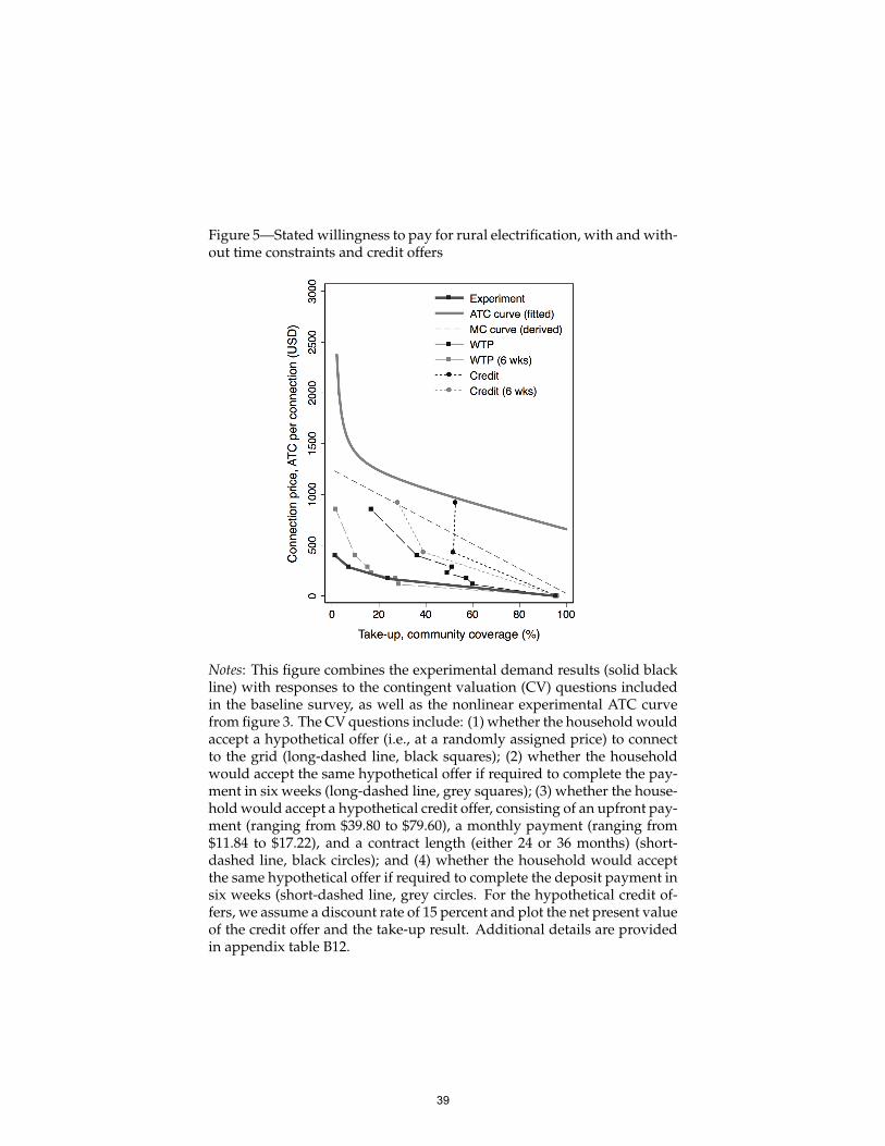
Figure 5—Stated willingness to pay for rural electrification, with and with-out time constraints and credit offers

Notes: This figure combines the experimental demand results (solid blackline) with responses to the contingent valuation (CV) questions includedin the baseline survey, as well as the nonlinear experimental ATC curvefrom figure 3. The CV questions include: (1) whether the household wouldaccept a hypothetical offer (i.e., at a randomly assigned price) to connectto the grid (long-dashed line, black squares); (2) whether the householdwould accept the same hypothetical offer if required to complete the pay-ment in six weeks (long-dashed line, grey squares); (3) whether the house-hold would accept a hypothetical credit offer, consisting of an upfront pay-ment (ranging from $39.80 to $79.60), a monthly payment (ranging from$11.84 to $17.22), and a contract length (either 24 or 36 months) (short-dashed line, black circles); and (4) whether the household would acceptthe same hypothetical offer if required to complete the deposit payment insix weeks (short-dashed line, grey circles. For the hypothetical credit of-fers, we assume a discount rate of 15 percent and plot the net present valueof the credit offer and the take-up result. Additional details are providedin appendix table B12.

39

Table 1—Differences between electricity grid unconnected vs. grid connected householdsat baseline

Unconnected Connected p-value of diff.

(1) (2) (3)

Panel A: Household head (respondent) characteristics

Female (%) 62.9 58.6 0.22

Age (years) 52.3 55.8 < 0.01

Senior citizen (%) 27.5 32.6 0.11

Attended secondary schooling (%) 13.3 45.1 < 0.01

Married (%) 66.0 76.7 < 0.01

Not a farmer (%) 22.5 39.5 < 0.01

Employed (%) 36.1 47.0 < 0.01

Basic political awareness (%) 11.4 36.7 < 0.01

Has bank account (%) 18.3 60.9 < 0.01

Monthly earnings (USD) 16.9 50.6 < 0.01

Panel B: Household characteristics

Number of members 5.2 5.3 0.76

Youth members (age ≤ 18) 3.0 2.6 0.01

High-quality walls (%) 16.0 80.0 < 0.01

Land (acres) 1.9 3.7 < 0.01

Distance to transformer (m) 356.5 350.9 0.58

Monthly (non-charcoal) energy (USD) 5.5 15.4 < 0.01

Panel C: Household assets

Bednets 2.3 3.4 < 0.01

Sofa pieces 6.0 12.5 < 0.01

Chickens 7.0 14.3 < 0.01

Radios 0.35 0.62 < 0.01

Televisions 0.15 0.81 < 0.01

Sample size 2,289 215

Notes: Columns 1 and 2 report sample means for households that were unconnected andconnected at the time of the baseline survey. Column 3 reports p-value of the differencebetween the means. Basic political awareness indicator captures whether the householdhead was able to correctly identify the presidents of Tanzania, Uganda, and the UnitedStates. Monthly earnings (USD) includes the respondent’s profits from businesses andself-employment, salary and benefits from employment, and agricultural sales for the en-tire household. In the 2013 census of all unconnected households, just 5 percent of ruralhouseholds were connected to the grid. In our sample of respondents, we oversampled thenumber of connected households.

40

Table 2—Impact of grid connection subsidy on take-up of electricity connections

Interacted variable

High-qualitywalls

Monthlyearnings

(USD)

Attendedsecondary

school

Baselineelectrifica-

tionrate

Baselineneighborsconnected

Report ofblackoutin past 3

days

(1) (2) (3) (4) (5) (6) (7) (8)

T1: Low subsidy—29% discount 5.8∗∗∗ 5.9∗∗∗ 3.6∗∗ 4.8∗∗∗ 4.5∗∗∗ 5.6∗∗ 4.8∗∗ 6.1∗∗

(1.4) (1.5) (1.5) (1.5) (1.4) (2.2) (1.9) (2.6)

T2: Medium subsidy—57% discount 22.4∗∗∗ 22.9∗∗∗ 21.3∗∗∗ 20.9∗∗∗ 19.8∗∗∗ 21.4∗∗∗ 21.4∗∗∗ 18.7∗∗∗

(4.0) (4.0) (4.4) (4.1) (3.8) (6.2) (3.5) (5.1)

T3: High subsidy—100% discount 94.2∗∗∗ 95.0∗∗∗ 95.6∗∗∗ 95.6∗∗∗ 95.2∗∗∗ 97.5∗∗∗ 96.1∗∗∗ 95.1∗∗∗

(1.2) (1.3) (1.2) (1.3) (1.3) (1.7) (1.3) (2.4)

Interacted variable 0.3 -0.0 -1.0 0.1 0.1 -0.9

(1.4) (0.0) (1.5) (0.1) (0.1) (1.3)

T1 × interacted variable 12.3∗∗ 0.1∗ 10.2 0.1 0.2 -0.2

(6.1) (0.0) (7.0) (0.2) (0.2) (3.1)

T2 × interacted variable 8.8 0.1∗ 19.5∗∗∗ 0.3 0.3 7.6

(7.8) (0.1) (4.6) (1.2) (0.2) (7.8)

T3 × interacted variable -5.5 -0.0 -4.3 -0.5∗ -0.2 -0.2

(3.9) (0.0) (4.9) (0.3) (0.1) (2.8)

Household and community controls No Yes Yes Yes Yes Yes Yes Yes

Observations 2289 2176 2176 2164 2176 2176 2176 2176

R2 0.68 0.69 0.69 0.70 0.70 0.69 0.69 0.69

Notes: The dependent variable is an indicator variable (multiplied by 100) for household take-up, with a mean of 21.6. Take-up in the control groupis 1.3. Robust standard errors clustered at the community level in parentheses. Pre-specified household controls include the age of the householdhead, indicators for whether the household respondent attended secondary school, is a senior citizen, is not primarily a farmer, is employed, andhas a bank account, an indicator for whether the household has high-quality walls, and the number of chickens (a measure of assets) owned by thehousehold. Pre-specified community controls include indicators for the county, market status, whether the transformer was funded and installedearly on (between 2008 and 2010), community electrification rate at baseline, and community population. Monthly earnings (USD) includes therespondent’s profits from businesses and self-employment, salary and benefits from employment, and agricultural sales for the entire household.Interacted variables in columns 7 and 8 are the proportion of neighbors (i.e., within 200 meters) connected to electricity and an indicator for whetherany households in the community reported a recent blackout, respectively. Asterisks indicate coefficient statistical significance level (2-tailed): *P < 0.10; ** P < 0.05; *** P < 0.01.

41

Table 3—Estimated treatment effects on pre-specified and grouped outcomes

Control ITT TOT FDR q-val

(1) (2) (3) (4)

Panel A: Treatment effects on pre-specified outcomes

P1. Grid connected (%) 5.6 89.7∗∗∗ – –

[23.0] (1.4)

P2. Monthly electricity spending (USD) 0.16 2.00∗∗∗ 2.20∗∗∗ .001

[1.29] (0.18) (0.20)

P3. Household employed or own business (%) 36.8 5.1 4.5 .416

[38.8] (3.1) (3.4)

P4. Total hours worked last week 50.9 -2.8∗ -3.6∗∗ .167

[32.8] (1.5) (1.7)

P5. Total asset value (USD) 888 109 110 .540

[851] (108) (120)

P6. Ann. consumption of major food items (USD) 117 -3 -5 .548

[92] (6) (7)

P7. Recent health symptoms index 0 -0.03 -0.05 .548

[1] (0.06) (0.07)

P8. Normalized life satisfaction 0 0.12∗∗ 0.13∗ .179

[1] (0.06) (0.07)

P9. Political and social awareness index 0 -0.03 -0.02 .731

[1] (0.05) (0.05)

P10. Average student test Z-score 0 -0.08 -0.10 .540

[0.99] (0.10) (0.10)

Panel B: Mean treatment effects on grouped outcomes

G1. Economic Index (P3 to P6 outcomes) 0 0.06 0.03 –

[1] (0.08) (0.08)

G2. Non-Economic Index (P7 to P10 outcomes) 0 -0.01 -0.02 –

[1] (0.06) (0.07)

Notes: In panel A, we report treatment effects on ten pre-specified primary outcomes. Column 1 reportsmean values for the control group, with standard deviations in brackets. Column 2 reports coefficientsfrom separate ITT regressions in which the dependent variable (e.g., P1) is regressed on the high subsidytreatment indicator. The low and medium subsidy groups are excluded from these regressions. Samplesizes range from 1,397 to 1,461 for the P1 to P9 regressions and 960 for the P10 regression. Column 3 reportscoefficients from separate TOT (IV) regressions in which household electrification status is instrumentedwith the three subsidy treatment indicators. Sample sizes range from 2,090 to 2,180 for the P1 to P9 regres-sions, and 1,432 for the P10 regression. All specifications include the relevant set of pre-specified household,student, and community covariates. Column 4 reports the FDR-adjusted q-values associated with the co-efficient estimates in column 3. In panel B, we report mean treatment effects on outcomes grouped intoan economic and non-economic index; these two groupings of outcomes were not pre-specified. Robuststandard errors clustered at the community level in parentheses. Asterisks indicate coefficient statisticalsignificance level (2-tailed): * P < 0.10; ** P < 0.05; *** P < 0.01.

42

Table 4—Alternative estimates of household (HH) consumer surplus based on monthly consumption

Monthly consumption

Benchmark

5 kWh 5 kWh 40 kWh 75 kWhNewly connected + 10% annual Baseline connected Median connected

Consumer demand HH in sample growth HH in sample HH in Nairobielasticity (1) (2) (3) (4)

-0.45 49 110 391 733

-0.30 73 164 587 1,100

-0.15 147 329 1,173 2,200

Notes: Estimates of consumer surplus based on monthly electricity consumption levels ranging from 5kWh to 75 kWh, and consumer demand elasticities ranging from -0.15 to -0.45. Common assumptionsinclude a discount rate of 15%, an asset life of 30 years, a price of $0.12 per kWh, linear demand, zeroconsumer surplus from electricity without a grid connection, and a 188 day delay before obtaining anelectricity connection (as illustrated in appendix figure A1). The 40 kWh level in column 3 corresponds tomedian consumption level reported by connected households at baseline. See appendix table B7 for detailson the benchmark electricity consumption levels.

43

Table 5—Predicting cost (C), consumer surplus (CS), and net welfare (NW) per household using different approaches and assumptions

Experimental Alternative

approach approach

C CS NW CS NW Key assumption(s)

Main estimates 658 147 -511 147 -511

a) Income growth – +139 – Income growth of 3 percent per annum over 30 years(experimental approach); (based on demand curves in figure 2, panel B);Electricity consumption – – +182 Electricity consumption growth of 10 percent per annumgrowth (alternative approach) over 30 years (see table 4, column 2, row 3).

b) No credit constraints for – +301 – Stated WTP without time constraints (see figure 5)grid connections

c) No transformer breakdowns – +33 +19 Reduce likelihood of transformer breakdowns from 5.4to 0 percent (see appendix table B10).

d) No grid connection delays – +46 +26 Reduce waiting period from 188 to 0 days (see appendixfigure A1).

e) No construction cost leakage -140 – – Decrease total construction costs by 21.3 percent (seeappendix table B8).

Ideal scenario 518 665 148 374 -144

Notes: Main estimates of C, CS, and NW correspond to figure 4, panel B (for the experimental approach), and table 4, column 1, row 3 (forthe alternative approach). Appendix table B13 includes an additional row to account for the consumer surplus associated with baselineconnected households.

44