TRITA-MEKTechnical Report 1999:16

ISSN 0348- 467XISRN KTH/MEK/TR--99/16--SE

Experimental studies of zero pressure-gradientturbulent boundary layer flow

Jens M. Österlund

Doctoral Thesis

Stockholm, 1999

Royal Institute of Technology

Department of Mechanics

Experimental Studies of Zero Pressure-Gradient

Turbulent Boundary-Layer Flow

by

Jens M. Osterlund

Department of Mechanics

December 1999Technical Reports from

Royal Institute of TechnologyDepartment of Mechanics

SE-100 44 Stockholm, Sweden

Typsatt i AMS-LATEX med KTHs thesis-stil.

Akademisk avhandling som med tillstand av Kungliga Tekniska Hogskolan iStockholm framlagges till offentlig granskning for avlaggande av teknologiedoktorsexamen fredagen den 17:e december 1999 kl 10.15 i sal D3, KTH, Val-hallavagen 79, Stockholm.

c© Jens M. Osterlund 1999

Norstedts tryckeri, Stockholm 1999

Jens M. Osterlund 1999 Experimental studies of zero pressure-gradient turbu-lent boundary layer flowDepartment of Mechanics, Royal Institute of TechnologySE-100 44 Stockholm, Sweden

Abstract

This thesis deals with the problem of high Reynolds number zero pressure-gradient turbulent boundary layers in an incompressible flow without any ef-fects of heat-transfer. The zero-pressure gradient turbulent boundary layer isone of the canonical shear flows important in many applications and of largetheoretical interest. The investigation was carried out through an experimentalstudy in the MTL wind-tunnel at KTH, where the fluctuating velocity com-ponents and the fluctuating wall-shear stress in a turbulent boundary layerwere measured using hot-wire and hot-film anemometry. Attempts were madeto answer some basic and “classical” questions concerning turbulent boundaryboundary layers.

The classical two layer theory was confirmed and constant values of theslope of the logarithmic overlap region (i.e. the von Karman constant) and theadditive constants were found and estimated to κ = 0.38, B = 4.1 and B1 = 3.6(δ = δ95). The inner limit of overlap region was found to scale on the viscouslength scale (ν/uτ) and was estimated to be y+ = 200, i.e. considerably furtherout compared to previous knowledge. The outer limit of the overlap region wasfound to scale on the outer length scale and was estimated to be y/δ = 0.15.This also means that a universal overlap region only can exist for Reynoldsnumbers of at least Reθ ≈ 6000. The values of the newly determined limitsexplain the Reynolds number variation found in some earlier experiments.

Measurements of the fluctuating wall-shear stress using the hot-wire-on-the-wall technique and a MEMS hot-film sensor show that the turbulence in-tensity τr.m.s./τw is close to 0.41 at Reθ ≈ 9800.

A numerical and experimental investigation of the behavior of double wireprobes were carried out and showed that the Peclet number based on wireseparation should be larger than about 50 to ensure an acceptably low level ofthermal interaction.

Results are presented for two-point correlations between the wall-shearstress and the streamwise velocity component for separations in both the wall-normal-streamwise plane and the wall-normal-spanwise plane. Turbulence pro-ducing events are further investigated using conditional averaging of isolatedshear-layer events. Comparisons are made with results from other experimentsand numerical simulations.

Descriptors: Fluid mechanics, turbulence, boundary layers, high Reynoldsnumber, zero-pressure gradient, hot-wire, hot-film anemometry, oil-film inter-ferometry, structures, streak spacing, micro-electro-mechanical-systems.

Preface

This thesis is an experimental study of high Reynolds number zero pressure-gradient turbulent boundary layer flow and is based on the following papers.

Paper 1. Osterlund, J. M., Johansson, A. V., Nagib, H. M. & Hites, M. H.1999 A note on the overlap region in turbulent boundary layers. Accepted forpublication in Phys. of Fluids.

Paper 2. Osterlund, J. M., Johansson, A. V., Nagib, H. M. & Hites, M. H.1999 Mean-flow characteristics of High Reynolds Number Turbulent BoundaryLayers from Two Facilities. To be submitted.

Paper 3. Osterlund, J. M. & Johansson, A. V. 1999 Turbulence Statistics ofZero Pressure-Gradient Turbulent Boundary Layers. To be submitted.

Paper 4. Bake, S. & Osterlund, J. M. 1999 Measurements of skin-frictionfluctuations in turbulent boundary layers with miniaturized wall-hot-wires andhot-films. Submitted to Phys. of Fluids..

Paper 5. Osterlund, J. M. & Johansson, A. V. 1994 Dynamic behavior ofhot-wire probes in turbulent boundary layers. Published in Advances in tur-bulence V, 398–402, 1995.

Paper 6. Osterlund, J. M., Lindgren, B. & Johansson, A. V. 1999 Structuresin zero pressure-gradient turbulent boundary layers. To be submitted.

Paper 7. Osterlund, J. M. & Johansson, A. V. 1999 Turbulent BoundaryLayer Experiments in the MTL Wind-Tunnel.

v

vi

Contents

Preface v

Chapter 1. Introduction 1

Chapter 2. Basic concepts 32.1. Boundary layer equations 42.2. Inner region 52.3. Outer region 52.4. Overlap region 62.5. Similarity description of the outer layer 7

Chapter 3. Experiments 103.1. History 103.2. Experimental set-up 103.3. Results 12

Chapter 4. Concluding Remarks 22

Acknowledgments 23

References 24

Paper 1 29

Paper 2 39

Paper 3 59

Paper 4 95

Paper 5 109

Paper 6 119

Paper 7 141

vii

viii

CHAPTER 1

Introduction

Whenever a fluid flows over a solid body, such as the hull of a ship or an aircraft,frictional forces retard the motion of the fluid in a thin layer close to the solidbody. The development of this layer is a major contributor to flow resistanceand is of great importance in many engineering problems.

The concept of a boundary layer is due to Prandtl (1904) who showed thateffects of friction within the fluid (viscosity) are present only in a very thin layerclose to the surface. If the flow velocity is high enough the flow in this layerwill eventually become unordered, swirling and chaotic or simply described asbeing turbulent. The transition from laminar to turbulent flow state was firstinvestigated by Reynolds (1883) who made experiments on the flow of water inglass tubes visualizing the flow state using ink as a passive marker. He foundthat the flow state was determined solely by a non-dimensional parameter thatis since then called the Reynolds number. The Reynolds number is a measureof the ratio between inertial and viscous forces in the flow, i.e. a high Reynoldsnumber flow is dominated by inertial forces.

The motion of a fluid is governed by the Navier-Stokes equations, namedafter Navier and Stokes who first formulated them in 1845. The Navier-Stokesequations are nonlinear and time dependent partial differential equations andonly a few analytical solutions exist for simple flows. No analytical solutionsexist for turbulent flows and to solve the equations for turbulent flows one hasto do numerical simulations. The computational effort increases rapidly withincreasing Reynolds number and for most practical engineering flow cases itis not possible to solve the full problem numerically even with todays mostpowerful super-computers. Therefore, one usually makes a simplification ofthe problem by splitting the velocity field into a mean and a fluctuating part,as first done by Reynolds (1895), and averaging the equations over time. Theresulting statistical description is the Reynolds averaged equations. This newset of equations is not closed, new terms appears in the averaging processand they need to be modeled. The statistical quantities needed in models canbe determined from simple low Reynolds number flows using direct numericalsimulations (DNS) or from experiments.

The Reynolds number in typical engineering applications with boundarylayer flow are often several orders of magnitude larger than what is possible

1

2 1. INTRODUCTION

DNS

102

103

104

105

106

107

108

Reθ

Car Ship & Aircraft

AtmosphereWind-tunnel

Figure 1.1. Typical Reynolds number in applications andattainable in lab facilities and simulations.

to achieve in direct numerical simulations or even compared to what is achiev-able in most experiments, see figure 1.1. Therefore, there is a gap in Reynoldsnumber between practical applications and the experiments which form thebasis for our knowledge of turbulence and turbulence modeling. Experimentsat high Reynolds number is therefore of primary importance to reveal Rey-nolds number trends that might have a large influence in many fluid dynamicapplications.

In the present study experiments on turbulent boundary layer flow withzero-pressure-gradient have been performed using hot-wire and hot-film mea-surement techniques. The goal was to extend the current knowledge of tur-bulent flows into high Reynolds number regime and to generate a databaseavailable to the research community.

CHAPTER 2

Basic concepts

y

z x

U

δU

Figure 2.1. Turbulent boundary layer with thickness δ andfree-stream velocity U∞ (vertical scale greatly expanded).

We here consider a turbulent flow in the immediate vicinity of a wall gen-erated by the uniform flow of a free-stream (with the velocity U∞) of a viscousincompressible fluid. The origin of the co-ordinate axes is placed at the leadingedge of the wall. The x-axis is oriented in the streamwise direction, the y-axis in the wall normal direction and the z-axis in the direction parallel to theleading edge, see figure 2.1. The wall is considered to be infinitely wide in thespanwise (z) direction and infinitely long in the streamwise (x) direction. Theflow conditions in the spanwise direction are uniform, in the statistical sense,with respect to the z-axis.

The flow is governed by the incompressible Navier-Stokes equations andthe continuity equation, which are given by

∂Ui

∂t+ Uj

∂Ui

∂xj= −1

ρ

∂P

∂xi+ ν

∂2Ui

∂x2j(2.1)

∂Ui

∂xi= 0 (2.2)

where Ui is the velocity vector, P is the pressure, and ρ and ν are the den-sity and kinematic viscosity of the fluid. Summation is implied over repeatedindices.

In the turbulent boundary layer the velocity components fluctuate ran-domly with respect to time and space around a mean value. This leads naturallyto the Reynolds decomposition of the velocity into a mean and a fluctuating

3

4 2. BASIC CONCEPTS

part. The velocity components for, the zero pressure-gradient boundary layer,in the different co-ordinate directions can thus be introduced, in the streamwisedirection

U(x, y, z, t) = U(x, y) + u(x, y, z, t), (2.3)

in the wall normal direction

V (x, y, z, t) = V (x, y) + v(x, y, z, t), (2.4)

and in the spanwise direction

W (x, y, z, t) = w(x, y, z, t), (2.5)

where the mean values are designated by an overbar and the fluctuating partby small letters. The same kind of decomposition is also used for the pressure

P (x, y, z, t) = P (y) + p(x, y, z, t) (2.6)

where the x dependence for P disappears by definition of the problem.For statistically steady turbulence averaging can be done either in the

homogeneous z direction or as a time average. In the present case the averagedvalue of a quantity is simply defined by

Q(x, y) = limT→∞

1T

∫ T

0

Q(x, y, z, t′)dt′ (2.7)

where the z dependence disappears because it is a homogeneous direction.

2.1. Boundary layer equations

Equations for the flow in the boundary layer are derived by insertion of theReynolds decomposition (2.3–2.5) into the Navier-Stokes equations 2.1 andsubsequent averaging yield the Reynolds averaged equations and the meancontinuity equation. 1 With the standard boundary layer approximations ofnegligible streamwise diffusion and constant pressure through the boundarylayer we obtain

U∂U

∂x+ V

∂U

∂y=

∂

∂y

(−uv + ν

∂U

∂y

)(2.8)

∂U

∂x+∂V

∂y= 0. (2.9)

The corresponding boundary conditions are

U(x, y = 0) = V (x, y = 0) = 0, (2.10)

U(x, y →∞) = U∞. (2.11)

This set of equations are indeterminate since there are more unknowns thanequations. This is known as the closure problem and additional relations or

1The analysis below was worked out jointly with prof. A. Johansson

2.3. OUTER REGION 5

hypotheses concerning the Reynolds stress −uv is needed to close this set ofequations.

Full similarity of the mean velocity profile, like the solutions for a laminarboundary layer, does not exist for the turbulent boundary layer. Instead, weseek similarity solutions for the velocity profiles in the inner and outer regionsof the boundary layer separately.

In the works of von Karman (1921, 1930), Prandtl (1927, 1932) and Mil-likan (1938) we find the classical theories for the turbulent boundary layer.Discussions of the classical theories can be found in Hinze (1975), Tennekes &Lumely (1972), Schlichting (1979) and Landahl & Mollo-Christensen (1987).There exists numerous refinements and competing theories in the literature andthe works of Coles (1956, 1962), Clauser (1956) Barenblatt (1993); Barenblatt& Prostokishin (1993); Barenblatt & Chorin (1999), George et al. (1997), Rotta(1950, 1962) and Zagarola et al. (1997); Zagarola & Smits (1998b,a), may beconsulted.

2.2. Inner region

The inner layer was first treated in the classical work by Prandtl (1932). Wedefine the governing length scale to be l∗ = ν/uτ , where u2τ = τw/ρ, τw is thewall shear stress, and derive a normalized wall distance y+ = y/l∗ = yuτ/ν .We assume outer geometrical restrictions (i.e. the outer length scale) to be ofnegligible influence sufficiently close to the wall, and assume the velocity andReynolds shear stress profiles to be universal functions of y+

U

uτ= f(y+) (2.12)

and

−uvu2τ

= g(y+). (2.13)

It is easily seen that the leading order balance obtained from the boundarylayer equations 2.8 is given by

0 = f ′′ + g′, (2.14)

which can be integrated once

f ′(y+) = −g(y+) + f ′(0) = −g(y+) + 1 (2.15)

which is seen to be compatible with the ‘law-of-the-wall’ assumptions 2.12 and2.13.

2.3. Outer region

For the outer layer description we define a governing length scale ∆, where ∆is some measure of the boundary layer thickness. A normalized wall distance

6 2. BASIC CONCEPTS

can be formed as η = y/∆. Assume that we can expand the normalized meanvelocity in a straight forward asymptotic expansion

U

U∞= F (η, Re∗) ∼ F0(η) + ε1(Re∗)F1(η) + ε2(Re∗)F2(η) + . . . (2.16)

where Fi are of order unity and εi are gauge functions such that εn+1 = o(εn),see e.g. Hinch (1991). The gauge functions are assumed to approach zero asthe Reynolds number Re∗ tends to infinity. Also assume

−uvu2τ

= G0(η) + h.o.t. (2.17)

If the velocity scale for the normalization of the Reynolds shear stress is leftopen, or chosen as different from uτ (see George et al. 1997) consistency wouldrequire that the ratio uτ/U∞ has to be assumed to approach a constant atinfinite Reynolds numbers.

2.4. Overlap region

For (infinitely) large Reynolds numbers the description (2.12,2.13) for y+ →∞should coincide with that given by (2.16,2.17) for η → 0. This is the classicaltwo-layer hypothesis of Millikan (1938). Hence, for large enough Reynoldsnumbers there should be an overlap region

l∗ y ∆ (2.18)

where both descriptions are valid simultaneously. The matching of the Rey-nolds shear stress simply gives that g and G0 should be constant (and equal)in the overlap region.

In the classical approach for the matching of the velocity we first constructthe normalized velocity gradient

y

uτ

∂U

∂y. (2.19)

This non-dimensional measure should be the same in the outer and the innerlayer description in the overlap region, i.e.

y

uτ

∂U

∂y= y+f ′(y+) =

U∞uτ

ηF ′0(η) + ε1

U∞uτ

ηF ′1(η) = const. (2.20)

From this approach we get the overlap velocity distribution given by

y+f ′(y+) = const =1κ

(2.21)

resulting in the log-law

f =1κ

ln y+ + B (2.22)

2.5. SIMILARITY DESCRIPTION OF THE OUTER LAYER 7

and for both sides of (2.20) to be of the same order of magnitude we get

F ′0 = 0 ⇒ F0 = const(= 1) (2.23)

and

ε1 =uτU∞

(2.24)

which introduced in (2.20) gives

ηF ′1 = const =

1κ

(2.25)

⇒ F1 =1κ

lnη −B1 (2.26)

or equivalently

U∞ − U

uτ= − 1

κlnη +B1. (2.27)

The log-law (2.22) together with the matching of the shear stress is indeedcompatible with the integrated form of the boundary layer equation in ‘innersimilarity form’, i.e. eq.(2.15), as y+ → ∞ (g → 1 as y+ →∞).

2.5. Similarity description of the outer layer

From the above analysis we get the outer layer description (with εn = εn1 ) as

U

U∞= 1 + γF1(η) + γ2F2(η) +O(γ3), (2.28)

where

γ =uτU∞

. (2.29)

Integrating the expression (2.28) from η = 0 to infinity yields

∆ =δ∗γ

{− 1∫ ∞

0F1dη

+ γ

∫ ∞0F2dη(∫∞

0F1dη

)2 + O(γ2)

}(2.30)

where we have used the definition of the displacement thickness (and thatη = y/∆). We can here choose the definition of ∆ such that∫ ∞

0

F1dη = −1 (2.31)

which hence gives that

∆ =δ∗γ

{1 + γ

∫ ∞

0

F2dη +O(γ2)}. (2.32)

To leading order this is the Clauser-Rotta lengthscale (Rotta 1950; Clauser1956).

8 2. BASIC CONCEPTS

We wish to reformulate the boundary layer equation in similarity form byuse of the expression (2.28) and the definition of ∆ (eq. 2.32). For this purposewe need to estimate duτ/dx and d∆/dx. By combining (2.22) with (2.28,2.26)we obtain the logarithmic friction law

U∞uτ

=1κ

ln∆uτν

+B +B1 , (2.33)

from which we readily derive∆uτ

duτdx

/d∆dx

= O (γ) . (2.34)

In estimating d∆/dx we first remember that for a zero pressure-gradient tur-bulent boundary layer we have

dθ

dx=

(uτU∞

)2

= γ2 (2.35)

where θ is the momentum loss thickness

θ =∫ ∞

0

U

U∞

(1− U

U∞

)dy (2.36)

which by use of (2.28) and (2.32) can be expressed as

θ

δ∗= 1− γ

∫ ∞

0

F 21 dη +O(γ2) (2.37)

Hence the contributions from F2 vanish to order γ in this expression and wenote that the shape factor H12 = δ∗/θ can be expressed as

H12 =[1− γ

∫ ∞

0

F 21 dη

]−1+O(γ2) (2.38)

i.e. the shape factor will approach unity (from above) as the Reynolds numbertends to infinity (uτ/U∞ → 0). The relation (2.38) is also consistent with thevariation found for the shape factor (see figure 17 of paper 7). From (2.37) weobtain by use of (2.34), (2.35)

dδ∗dx

=dθ

dx(1 +O(γ)) = γ2 +O

(γ3

), (2.39)

d∆dx

=1γ

dδ∗dx

(1 +O(γ)) = γ +O(γ2

). (2.40)

For the reformulation of the boundary layer equation we need∂η

∂x= − η

∆d∆dx

= − η

δ∗

(γ2 +O

(γ3

)), (2.41)

∂η

∂y=

1∆

=1δ∗

(γ +O

(γ2

)). (2.42)

2.5. SIMILARITY DESCRIPTION OF THE OUTER LAYER 9

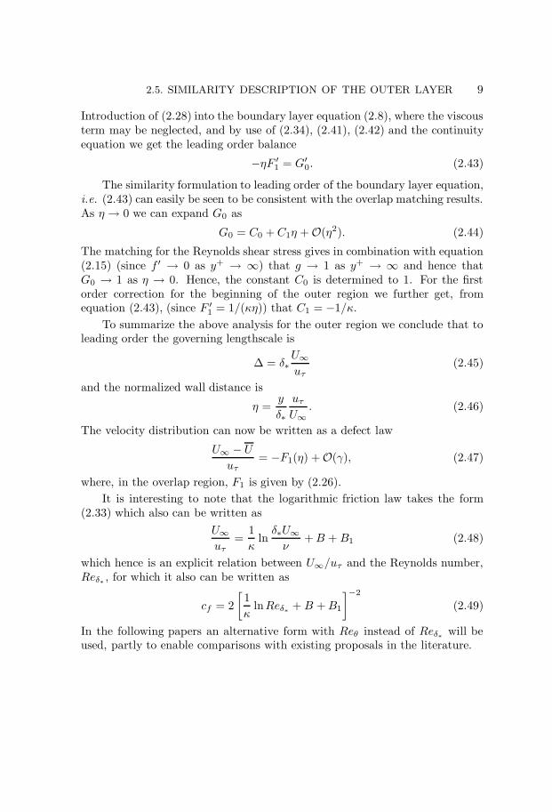
Introduction of (2.28) into the boundary layer equation (2.8), where the viscousterm may be neglected, and by use of (2.34), (2.41), (2.42) and the continuityequation we get the leading order balance

−ηF ′1 = G′

0. (2.43)

The similarity formulation to leading order of the boundary layer equation,i.e. (2.43) can easily be seen to be consistent with the overlap matching results.As η→ 0 we can expand G0 as

G0 = C0 +C1η +O(η2). (2.44)

The matching for the Reynolds shear stress gives in combination with equation(2.15) (since f ′ → 0 as y+ → ∞) that g → 1 as y+ → ∞ and hence thatG0 → 1 as η → 0. Hence, the constant C0 is determined to 1. For the firstorder correction for the beginning of the outer region we further get, fromequation (2.43), (since F ′

1 = 1/(κη)) that C1 = −1/κ.To summarize the above analysis for the outer region we conclude that to

leading order the governing lengthscale is

∆ = δ∗U∞uτ

(2.45)

and the normalized wall distance is

η =y

δ∗

uτU∞

. (2.46)

The velocity distribution can now be written as a defect law

U∞ − Uuτ

= −F1(η) +O(γ), (2.47)

where, in the overlap region, F1 is given by (2.26).It is interesting to note that the logarithmic friction law takes the form

(2.33) which also can be written asU∞uτ

=1κ

lnδ∗U∞ν

+B + B1 (2.48)

which hence is an explicit relation between U∞/uτ and the Reynolds number,Reδ∗ , for which it also can be written as

cf = 2[

1κ

lnReδ∗ + B +B1

]−2(2.49)

In the following papers an alternative form with Reθ instead of Reδ∗ will beused, partly to enable comparisons with existing proposals in the literature.

CHAPTER 3

Experiments

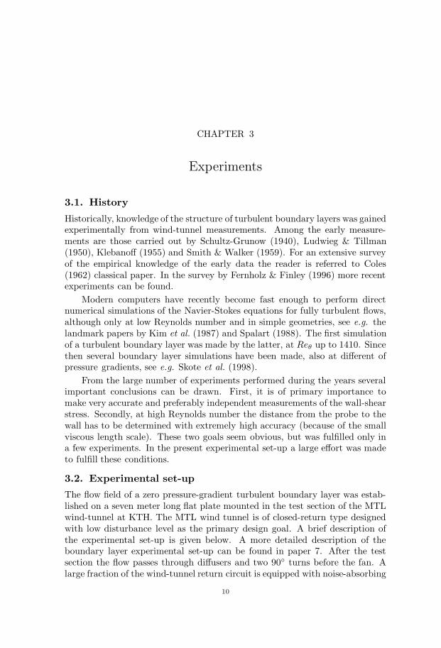
3.1. History

Historically, knowledge of the structure of turbulent boundary layers was gainedexperimentally from wind-tunnel measurements. Among the early measure-ments are those carried out by Schultz-Grunow (1940), Ludwieg & Tillman(1950), Klebanoff (1955) and Smith & Walker (1959). For an extensive surveyof the empirical knowledge of the early data the reader is referred to Coles(1962) classical paper. In the survey by Fernholz & Finley (1996) more recentexperiments can be found.

Modern computers have recently become fast enough to perform directnumerical simulations of the Navier-Stokes equations for fully turbulent flows,although only at low Reynolds number and in simple geometries, see e.g. thelandmark papers by Kim et al. (1987) and Spalart (1988). The first simulationof a turbulent boundary layer was made by the latter, at Reθ up to 1410. Sincethen several boundary layer simulations have been made, also at different ofpressure gradients, see e.g. Skote et al. (1998).

From the large number of experiments performed during the years severalimportant conclusions can be drawn. First, it is of primary importance tomake very accurate and preferably independent measurements of the wall-shearstress. Secondly, at high Reynolds number the distance from the probe to thewall has to be determined with extremely high accuracy (because of the smallviscous length scale). These two goals seem obvious, but was fulfilled only ina few experiments. In the present experimental set-up a large effort was madeto fulfill these conditions.

3.2. Experimental set-up

The flow field of a zero pressure-gradient turbulent boundary layer was estab-lished on a seven meter long flat plate mounted in the test section of the MTLwind-tunnel at KTH. The MTL wind tunnel is of closed-return type designedwith low disturbance level as the primary design goal. A brief description ofthe experimental set-up is given below. A more detailed description of theboundary layer experimental set-up can be found in paper 7. After the testsection the flow passes through diffusers and two 90◦ turns before the fan. Alarge fraction of the wind-tunnel return circuit is equipped with noise-absorbing

10

3.2. EXPERIMENTAL SET-UP 11

Test section

Fan

Cooler

ContractionGrids

Stagnation chamber

Guide vanes

7m

Diffuser

Honecomb

Figure 3.1. Schematic of the MTL wind tunnel facility at KTH

walls to reduce acoustic noise. The high flow quality of the MTL wind-tunnelwas reported by Johansson (1992). For instance, the streamwise turbulence in-tensity was found to be less than 0.02%. The air temperature can be controlledwithin ±0.05 ◦C, which was very important for this study since the primarymeasurement technique was hot-wire/hot-film anemometry, where a constantair temperature during the measurement is a key issue. The test section hasa cross sectional area of 0.8 m (high) × 1.2 m (wide) and is 7 m long. Theupper and lower walls of the test section can be moved to adjust the pressuredistribution. The maximum variation in mean velocity distribution along theboundary layer plate was ±0.15%.

The plate is a sandwich construction of aluminum sheet metal and squaretubes in seven sections plus one flap and one nose part, with the dimensions 1.2m wide and 7 m long excluding the flap. The flap is 1.5 m long and is mountedin the first diffuser. This arrangement makes it possible to use the first 5.5 m ofthe plate for the experiment. One of the plate sections was equipped with twocircular inserts, one for a plexiglas plug where the measurements were carriedout, and one for the traversing system. The traversing system was fixed tothe plate to minimize vibrations and possible deflections. The distance to thewall from the probe was determined by a high magnification microscope. Theabsolute error in the determination of the wall distance was within ±5µm.

The boundary layer was tripped at the beginning of the plate and the two-dimensionality of the boundary layer was checked by measuring the spanwise

12 3. EXPERIMENTS

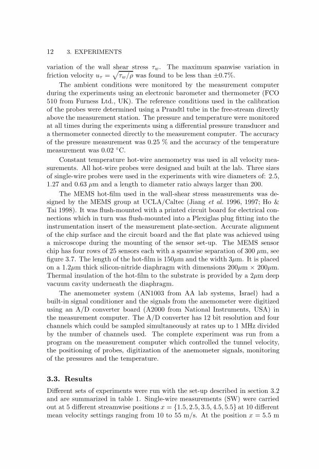
variation of the wall shear stress τw. The maximum spanwise variation infriction velocity uτ =

√τw/ρ was found to be less than ±0.7%.

The ambient conditions were monitored by the measurement computerduring the experiments using an electronic barometer and thermometer (FCO510 from Furness Ltd., UK). The reference conditions used in the calibrationof the probes were determined using a Prandtl tube in the free-stream directlyabove the measurement station. The pressure and temperature were monitoredat all times during the experiments using a differential pressure transducer anda thermometer connected directly to the measurement computer. The accuracyof the pressure measurement was 0.25 % and the accuracy of the temperaturemeasurement was 0.02 ◦C.

Constant temperature hot-wire anemometry was used in all velocity mea-surements. All hot-wire probes were designed and built at the lab. Three sizesof single-wire probes were used in the experiments with wire diameters of: 2.5,1.27 and 0.63 µm and a length to diameter ratio always larger than 200.

The MEMS hot-film used in the wall-shear stress measurements was de-signed by the MEMS group at UCLA/Caltec (Jiang et al. 1996, 1997; Ho &Tai 1998). It was flush-mounted with a printed circuit board for electrical con-nections which in turn was flush-mounted into a Plexiglas plug fitting into theinstrumentation insert of the measurement plate-section. Accurate alignmentof the chip surface and the circuit board and the flat plate was achieved usinga microscope during the mounting of the sensor set-up. The MEMS sensorchip has four rows of 25 sensors each with a spanwise separation of 300 µm, seefigure 3.7. The length of the hot-film is 150µm and the width 3µm. It is placedon a 1.2µm thick silicon-nitride diaphragm with dimensions 200µm × 200µm.Thermal insulation of the hot-film to the substrate is provided by a 2µm deepvacuum cavity underneath the diaphragm.

The anemometer system (AN1003 from AA lab systems, Israel) had abuilt-in signal conditioner and the signals from the anemometer were digitizedusing an A/D converter board (A2000 from National Instruments, USA) inthe measurement computer. The A/D converter has 12 bit resolution and fourchannels which could be sampled simultaneously at rates up to 1 MHz dividedby the number of channels used. The complete experiment was run from aprogram on the measurement computer which controlled the tunnel velocity,the positioning of probes, digitization of the anemometer signals, monitoringof the pressures and the temperature.

3.3. Results

Different sets of experiments were run with the set-up described in section 3.2and are summarized in table 1. Single-wire measurements (SW) were carriedout at 5 different streamwise positions x = {1.5, 2.5, 3.5, 4.5, 5.5} at 10 differentmean velocity settings ranging from 10 to 55 m/s. At the position x = 5.5 m

3.3. RESULTS 13

Reθ Quantity Pos. (x) Ref.

SW 2500–27300 U 1.5–5.5 paper 1 & 2XW 6900–22500 U, V 5.5 paper 3VW 6900–22500 U, W 5.5 paper 3

MEMS-WW 9700 τw 5.5 paper 4MEMS-MEMS 9700 τw, τw(∆z) 5.5 paper 6MEMS-SW 1 9700 τw, U(∆x, ∆y) 5.5 paper 6MEMS-SW 2 9700 τw, U(∆y, ∆z) 5.5 paper 6

Table 1. Overview of the different sets of experiments.

experiments with three different probe sizes were also conducted. An X-probewas used at the position x = 5.5 m for measurements (XW) of the simultane-ous streamwise U and wall-normal velocity V components. The simultaneousstreamwise and spanwise W velocity components were measured (VW) using aV-probe. The MEMS hot-film sensor, with 25 individual hot-films distributedin the spanwise direction, was utilized to measure the simultaneous skin-frictionin two points at different spanwise separations. The MEMS hot-film sensor wasalso used to measure simultaneously the skin-friction and the streamwise ve-locity separated in either the x-y plane (MEMS-SW 1) or separated in the y-zplane (MEMS-SW 2).

The mean skin friction was determined using oil-film interferometry andthe near-wall method. The result is shown in figure 3.2. A fit to cf by a variantof the logarithmic skin friction law, namely

cf = 2[

1κ

ln(Reθ) +C

]−2, (3.50)

was made for each of the data sets. The value of the von Karman constantdetermined in this way was κ = 0.384 and the additive constant was found tobe C = 4.08, see paper 2. The resulting logarithmic skin-friction laws agreevery well with each other and also with the correlation by Fernholz & Finley(1996).

The large set of single-wire measurements gave a unique possibility to in-vestigate topics such as the mean velocity scaling laws. In figures 3.3 and3.4 the mean velocity profiles from single-wire measurements in the Reynoldsnumber range 2500 < Reθ < 27700 are shown in inner and outer scaling. Alsoshown in the figures are the logarithmic laws with the newly determined valuesof the log-law constants κ = 0.38, B = 4.1 and B1 = 3.6 (paper 1).

The scaling law in the overlap region was investigated using the normalizedslope of the mean velocity profile,

Ξ =

(y+

dU+

dy+

)−1

. (3.51)

14 3. EXPERIMENTS

Reθ

cf

0 0.5 1 1.5 2 2.5 3

x 104

2

2.5

3

3.5x 10

-3

Fernholz & Finley (1996)Oil-film (series 1)Oil-film (series 2)Oil-film fitNear-wall fitNear-wall, x = 1.5 mNear-wall, x = 2.5 mNear-wall, x = 3.5 mNear-wall, x = 4.5 mNear-wall, x = 5.5 mNear-wall, x = 5.5 m

Figure 3.2. Skin-friction coefficient cf using the oil-film andnear wall methods (paper 7), shown with best-fit logarithmicfriction laws from equation 3.50 and the correlation by Fern-holz & Finley (1996).

In a logarithmic region of the profiles Ξ is constant and equal to κ. The value ofΞ was calculated by taking an average of the individual profiles at a constantwall distance in inner scaling while omitting the part of the profiles whereη > Mo. Similarly, the profiles were again averaged at constant outer-scaleddistances from the wall for y+ > Mi. The parameters Mi and Mo are theinner and outer limits of the overlap region. In Figure 3.5, the averaged Ξis shown together with error bars representing a 95% confidence interval. Aregion where a nearly constant Ξ very accurately represents the data is evidentin both figures. This clearly supports the existence of a logarithmic overlapregion within the appropriate range of the parameters Mi and Mo. The choiceof the appropriate limits was subsequently selected based on the y values wherethe error bar deviates significantly from the horizontal line in the figures. Thiswas based on an iteration of the limits until a consistent result was obtained.The resulting values for the inner and outer limits areMi ≈ 200 and Mo ≈ 0.15,respectively.

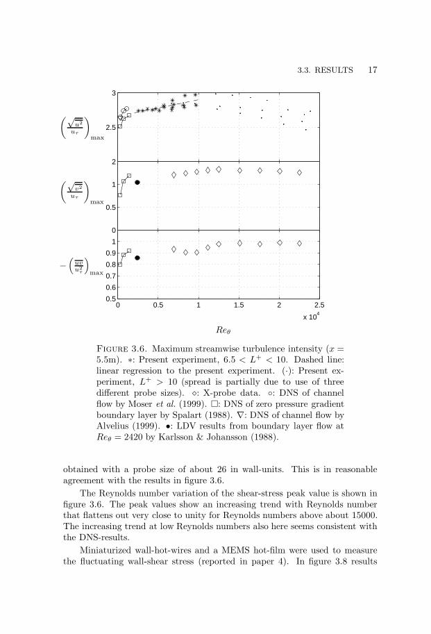
Statistical quantities, such as the turbulence intensities, were investigatedin paper 3. The peak values of the absolute and relative intensities are shown infigure 3.6. Also shown in figure 3.6 are corresponding values obtained from di-rect numerical simulations by Spalart (1988), Moser et al. (1999) and Alvelius

3.3. RESULTS 15

100

101

102

103

104

0

5

10

15

20

25

30

35

U+

y+

Figure 3.3. Profiles of the mean velocity in inner-law scaling.2530 < Reθ < 27300. Dash-dotted line: 1

0.38 ln y+ + 4.1.

10-4

10-3

10-2

10-1

0

5

10

15

20

25

30

U∞−Uuτ

y/∆

Figure 3.4. Profiles of the mean velocity in outer-law scaling.Log-law constants κ = 0.38 and B∆

1 = 1.62. 2530 < Reθ <27300

16 3. EXPERIMENTS

100 200 300 400 500 600 700 800 900 10000.15

0.2

0.25

0.3

0.35

0.4

0.45

0.5

y+

Ξ

Figure 3.5. Normalized slope of mean profile, Ξ, shown ininner scaling; only the part of the profiles in which η < 0.15was used and the horizontal line corresponds to κ = 0.38

(1999), where the first is a boundary layer simulation and the last two arechannel flow simulations. One should keep in mind in the comparisons withthe DNS-data that the channel flow has a somewhat different character, whereReynolds number effects on turbulence production etc. can be related to therelative influence of the pressure gradient. This can partly be seen from theintegrated form of the mean flow equation. An increasing trend is visible infigure 3.6. The increase in

√u2/uτ is about 7% for the present data in this

Reynolds number range but the increase in√u2/U is only about half of that.

For√u2/uτ one can observe a significant difference between the channel flow

and boundary layer DNS data. The present set of experimental data smoothlyextends the boundary layer DNS-results to substantially higher Reynolds num-bers, with a continued increase of the maximum intensity. One could expect alevelling off to occur at high Reynolds numbers. From the results in figure 3.6it is not really possible to determine an asymptotic level of (

√u2/uτ)max but

it can be judged to be at least 2.9. The peak value of v2 is seen in figure 3.6 toincrease with the Reynolds number in a manner similar to the variation in thepeak value for u2. At the high Reynolds number end a decreasing trend is seenthat is probably due to spatial averaging effects. The increase in (v2/uτ)maxfor Reθ < 13000 seems consistent with the low Reynolds number DNS-results.Fernholz & Finley (1996) reported max-values of about 1.4 for Reθ = 20920

3.3. RESULTS 17

Reθ

(√u2

uτ

)max

(√v2

uτ

)max

−(uvu2

τ

)max

2

2.5

3

0

0.5

1

0 0.5 1 1.5 2 2.5

x 104

0.5

0.6

0.7

0.8

0.9

1

Figure 3.6. Maximum streamwise turbulence intensity (x =5.5m). ∗: Present experiment, 6.5 < L+ < 10. Dashed line:linear regression to the present experiment. (·): Present ex-periment, L+ > 10 (spread is partially due to use of threedifferent probe sizes). �: X-probe data. ◦: DNS of channelflow by Moser et al. (1999). �: DNS of zero pressure gradientboundary layer by Spalart (1988). ∇: DNS of channel flow byAlvelius (1999). •: LDV results from boundary layer flow atReθ = 2420 by Karlsson & Johansson (1988).

obtained with a probe size of about 26 in wall-units. This is in reasonableagreement with the results in figure 3.6.

The Reynolds number variation of the shear-stress peak value is shown infigure 3.6. The peak values show an increasing trend with Reynolds numberthat flattens out very close to unity for Reynolds numbers above about 15000.The increasing trend at low Reynolds numbers also here seems consistent withthe DNS-results.

Miniaturized wall-hot-wires and a MEMS hot-film were used to measurethe fluctuating wall-shear stress (reported in paper 4). In figure 3.8 results

18 3. EXPERIMENTS

Figure 3.7. MEMS hot-film sensor chip from UCLA/Caltech(Jiang et al. 1996), mounted in the center of a printed circuitboard providing the electrical connections. A blow-up of oneof the vacuum insulated hot-films is also shown.

for the skin-friction intensity Tτw are presented, for all experiments performedin this investigation, against the active sensor length in viscous units. Thedata show a decrease in intensity for increasing probe dimensions as a result ofspatial averaging (see e.g. Johansson & Alfredsson 1983; Ligrani & Bradshaw1987). The limiting value of the turbulence intensity for small probe lengths ishere found to be about 0.41. For comparison the results from the wall-hot-wireexperiments at MIT in a turbulent boundary layer in air flow by Alfredssonet al. (1988) are also shown in figure 3.8 and show good agreement with thepresent data. The resulting intensity from the MEMS hot-film of 0.35 is morethan 10% too low and can probably be attributed to remaining heat losses inthe diaphragm that modifies the dynamic response compared to the static one.Still, the result represents a major improvement compared to previous findingsusing hot-films in air where values of about 0.1 are reported for the relativeintensity of the wall shear stress fluctuations. Also, the rapid development inMEMS technology will probably lead towards large improvements in the nearfuture. The wall-hot-wire of type 3, with the wire welded onto prongs flush withthe wall, show a behavior similar to the hot-film. The plausible explanationbeing that heat flux from the wire, which is only a few µm above the wall, ispartly absorbed by the wall and transferred back to the fluid, in a mechanismsimilar to that for the hot-film. A connected issue is that the sensitivity of

3.3. RESULTS 19

l+

Tτw

0 10 20 30 40 50 600.2

0.25

0.3

0.35

0.4

0.45

Figure 3.8. Turbulent skin friction intensity Tτw . Presentexperiments, ◦: WW1, MTL, +: WW3, MTL, ×: MHF, MTL,�: WW2, MTL, •: WW1, LaWiKa, �: WW2, LaWiKa,�: WW2, LaWiKa, �: WW2, LaWiKa, �: WW2, LaWiKa(for details see table 2 in paper 4). 2: experiment by Alfreds-son et al. (1988).

type 3 wall-hot-wires is very low due to damping resulting from the proximityof the wall.

Kline et al. (1967), showed that a significant part of the turbulence couldbe described in terms of deterministic events, and that in the close proximityof the wall the flow is characterized by elongated regions of low and high speedfluid of fairly regular spanwise spacing of about λ+ = 100. Sequences of orderedmotion occur randomly in space and time where the low-speed streaks beginto oscillate and to suddenly break-up into a violent motion, a “burst”. Kimet al. (1971) showed that the intermittent bursting process is closely related toshear-layer like flow structures in the buffer region. To obtain quantitative datato describe the structures a reliable method to identify bursts with velocity orwall-shear stress measurements is needed. Kovasznay et al. (1970) were the firstto employ conditional averaging, using a trigger, to study individual events suchas bursts or ejections. The triggering signal must be intermittent and closelyassociated with the event under study. Wallace et al. (1972) and Willmart& Lu (1972) introduced the uv quadrant splitting scheme. Blackwelder &Kaplan (1976) developed the VITA technique to form a localized measure of

20 3. EXPERIMENTS

∆z+

Rτwτw

0 50 100 150 200

-0.2

0

0.2

0.4

0.6

0.8

1

Figure 3.9. Spanwise correlation coefficient Rτwτw as a func-tion of ∆z+, Reθ = 9500. Present data, �: unfiltered,�: f+c = 1.3× 10−3, �: f+c = 2.6× 10−3, ◦: f+c = 5.3× 10−3,�: f+c = 7.9× 10−3, —: spline fit to ◦. DNS of channel flow,−−: Reτ = 590, − · −: Reτ = 385, · · · : Reτ = 180 (Kim et al.1987; Moser et al. 1999).

the turbulent kinetic energy and used it to detect shear-layer events. For acomprehensive overview of the literature in the field of coherent structures thereader is referred to the review article by Robinson (1991).

In paper 6 the mean spanwise separation between low-speed streaks inthe viscous sub-layer was investigated using a MEMS array of hot-films. Thespanwise cross correlation coefficient between the wall-shear stress signals

Rτwτw (∆z) =τw(z)τw(z + ∆z)

τ ′2w, (3.52)

obtained from two hot-films separated a distance ∆z+ in the spanwise directionwas used to estimate the mean streak spacing. At high Reynolds numbers con-tributions to the spanwise correlation coefficient from low frequency structuresoriginating in the outer region conceals the contributions from the streaks andno clear (negative) minimum is visible in figure 3.9 for the measured correlationcoefficient (shown as�). This behavior was found also by others, see e.g. Guptaet al. (1971). A trend is clearly visible in the relatively low Reynolds number

3.3. RESULTS 21

simulations by Kim et al. (1987) and Moser et al. (1999) where at their highReynolds number the minimum is less pronounced. In an attempt to reveal andpossibly obtain the streak spacing also from the high Reynolds number data inthe present experiment we applied a high-pass (Chebyshev phase-preserving)digital filter to the wall-shear stress signals before calculating the correlationcoefficient. This procedure reveals the content from the streaks and enhancesthe variation in the correlation coefficient. A variation of the cut-off frequencyrevealed no significant dependence of the position of the minimum on the cut-off. The cut-off frequency was chosen to damp out frequencies coming fromstructures larger than about 2500 viscous length scales corresponding to theboundary layer thickness. The filtered correlation is shown for different cut-offfrequencies in figure 3.9. The correlation decrease rapidly and a broad mini-mum is found at ∆z+ ≈ 55 giving a mean streak spacing of λ+ ≈ 110. Thecorrelation coefficient is close to zero for separations ∆z+ > 100.

CHAPTER 4

Concluding Remarks

Experimental results were presented for turbulent boundary layer measure-ments spanning over one decade in Reynolds number, 2500 < Reθ < 27000.

The classical two layer theory was confirmed and constant values of theslope of the logarithmic overlap region (i.e. von Karmans constant) and theadditive constants were found and estimated to κ = 0.38, B = 4.1 and B1 = 3.6(δ = δ95). The inner limit of overlap region was found to scale on the viscouslength scale (ν/uτ) and was estimated to be y+ = 200, i.e. considerably furtherout compared to previous knowledge. The outer limit of the overlap region wasfound to scale on the outer length scale and was estimated to be y/δ = 0.15.This means that a universal overlap region can only be expected for Reynoldsnumbers larger than Reθ ≈ 6000. The newly determined limits also explainthe Reynolds number variation found in some earlier experiments.

Measurements of the fluctuating wall-shear stress using the hot-wire-on-the-wall technique and a MEMS hot-film sensor show that the turbulence in-tensity τw/τr.m.s. is close to 0.41 at Reθ ≈ 9800. This was also substantiatedby near-wall single-wire measurements.

A numerical and experimental investigation of the behavior of double wireprobes were carried out and showed that the Peclet number based on wire sep-aration should be larger than about 50 to keep the interaction at an acceptablelevel.

Results are presented for two-point correlations between the wall-shearstress and the streamwise velocity component for separations in both the wall-normal-streamwise plane and the wall-normal-spanwise plane. Results are pre-sented for the streak spacing and the propagation velocity of near wall shearlayer events. Turbulence producing events are further investigated using condi-tional averaging of isolated events detected using the VITA technique. Compar-isons are made with results from other experiments and numerical simulations.

22

Acknowledgments

I would like to sincerely thank my supervisor Prof. Arne Johansson for accept-ing me as his student, imparting his knowledge and and guiding me throughthe maze of turbulence research. Arne has read and and given constructivecriticism an all manuscripts in this work.

I also would like to thank Prof. Henrik Alfredsson for innumerable helpfuldiscussions about fluid mechanics and especially turbulence experiments.

My thanks to Prof. Hassan Nagib at IIT, with whom I had the greatpleasure to work with during his stay at KTH. The enthusiastic and creativecomments from Hassan has been invaluable when finishing this work.

I also wish to thank Dr. Erik Lindborg for clarifying discussions on theanalysis of the boundary layer similarity analysis.

My special thanks go to my dear friend and former colleague AlexanderSahlin together with who I started out doing the experiments leading to thisthesis. Alexander’s sound knowledge of fluid dynamics has been invaluable helpthroughout this work.

Many thanks go to the faculty, my colleagues and fellow students at theDepartment of Mechanics for a pleasant, stimulating and inspiring atmosphere.Especially I want to thank my friends and room mates Torbjorn Sjogren andBjorn Lindgren who have made my time in the lab most enjoyable.

I wish to thank Marcus Gallstedt and Ulf Landen for help with design-ing and building many of the experiments and for skillful assistance in thelaboratory.

Last but not the least, I want to thank my parents and family for theirsupport and especially, Ulrika for your love.

Financial support from the Swedish Research Council for Engineering Science(TFR) and Swedish National Board for Industrial and Technical Development(NUTEK) is gratefully acknowledged.

23

References

Alfredsson, P. H., Johansson, A. V., Haritonidis, J. H. & Eckelmann, H.

1988 The fluctuation wall-shear stress and the velocity field in the viscous sub-layer. Phys. Fluids A 31, 1026–33.

Alvelius, K. 1999 Studies of turbulence and its modeling through large eddy- anddirect numerical simulation. PhD thesis, Department of Mechanics, Royal Insti-tute of Technology, Stockholm.

Barenblatt, G. I. 1993 Scaling laws for fully developed turbulent shear flows. part1. basic hypotheses and analysis. J. Fluid Mech. 248, 513–520.

Barenblatt, G. I. & Chorin, A. J. 1999 Self-similar intermediate structures inturbulent boundary layers at large reynolds numbers. PAM 755. Center for Pureand Applied Mathematics, University of California at Berkeley.

Barenblatt, G. I. & Prostokishin, V. M. 1993 Scaling laws for fully developedturbulent shear flows. part 2. processing of experimental data. J. Fluid Mech.248, 521–529.

Blackwelder, R. F. & Kaplan, R. E. 1976 On the wall structure of the turbulentboundary layer. J. Fluid Mech. 76, 89–112.

Clauser, F. H. 1956 The turbulent boundary layer. Advances Appl. Mech. 4, 1–51.

Coles, D. E. 1956 The law of the wake in the turbulent boundary layer. J. FluidMech. 1, 191–226.

Coles, D. E. 1962 The turbulent boundary layer in a compressible fluid. R 403-PR.The RAND Corporation, Santa Monica, CA.

Fernholz, H. H. & Finley, P. J. 1996 The incompressible zero-pressure-gradientturbulent boundary layer: An assessment of the data. Prog. Aerospace Sci. 32,245–311.

George, W. K., Castilio, L. & Wosnik, M. 1997 Zero-pressure-gradient turbulentboundary layer. Applied Mech. Reviews 50, 689–729.

Gupta, A. K., Laufer, J. & Kaplan, R. E. 1971 Spatial structure in the viscoussublayer. J. Fluid Mech. 50, 493–512.

Hinch, E. J. 1991 Perturbation methods. Cambridge University Press.

Hinze, J. O. 1975 Turbulence , 2nd edn. McGraw-Hill.

Ho, C.-M. & Tai, Y.-C. 1998 Micro-electro-mechanical-systems (MEMS) and fluidflows. Ann. Rev. Fluid Mech. 30, 579–612.

24

REFERENCES 25

Jiang, F., Tai, Y.-C., Gupta, B., Goodman, R., Tung, S., Huang, J. B. & Ho,

C.-M. 1996 A surface-micromachined shear stress imager. In 1996 IEEE MicroElectro Mechanical Systems Workshop (MEMS ’96), pp. 110–115.

Jiang, F., Tai, Y.-C., Walsh, K., Tsao, T., Lee, G. B. & Ho, C.-H. 1997 Aflexible mems technology and its first application to shear stress sensor skin.In 1997 IEEE Micro Electro Mechanical Systems Workshop (MEMS ’97), pp.465–470.

Johansson, A. V. 1992 A low speed wind-tunnel with extreme flow quality - designand tests. In Prog. ICAS congress 1992 , pp. 1603–1611. ICAS-92-3.8.1.

Johansson, A. V. & Alfredsson, P. H. 1983 Effects of imperfect spatial resolutionon measurements of wall-bounded turbulent shear flows. J. Fluid Mech. 137,409–421.

Karlsson, R. I. & Johansson, T. G. 1988 Ldv measurements of higher order mo-ments of velocity fluctuations in a turbulent boundary layer. In Laser Anemome-try in Fluid Mechanics . Ladoan-Instituto Superior Tecnico, 1096 L.C., Portugal.

von Karman, T. 1921 Ueber laminare un turbulente Reibung. Z. angew. Math.Mech. pp. 233–252, NACA TM 1092.

von Karman, T. 1930 Mechanische Aehnlichkeit und Turbulenz. Nachr. Ges. Wiss.Gottingen, Math. Phys. Kl. pp. 58–68, NACA TM 611.

Kim, H. T., Kline, S. J. & Reynolds, W. C. 1971 The production of turbulencenear a smooth wall in a turbulent boundary layer. J. Fluid Mech. 50, 133–160.

Kim, J., Moin, P. & Moser, R. 1987 Turbulence statistics in fully developed channelflow. J. Fluid Mech. 177, 133–166.

Klebanoff, P. S. 1955 Characteristics of turbulence in a boundary layer with zeropressure gradient. TR 1247. NACA.

Kline, S. J., Reynolds, W. C., Schraub, F. A. & Runstadler, P. W. 1967 Thestructure of turbulent boundary layers. J. Fluid Mech. 30, 741.

Kovasznay, L. G., Kibens, V. & Blackwelder, R. S. 1970 Large-scale motionin the intermittent region of a turbulent boundary layer. J. Fluid Mech. 41,283–325.

Landahl, M. T. & Mollo-Christensen, E. 1987 Turbulence and Random Pro-cesses in Fluid Mechanics . Cambridge University Press.

Ligrani, P. M. & Bradshaw, P. 1987 Spatial resolution and measurement of tur-bulence in the viscous sublayer using subminiature hot-wire probes. Experimentsin Fluids 5, 407–417.

Ludwieg, H. & Tillman, W. 1950 Investigations of the wall shearing stress inturbulent boundary layers. TM 1285. NACA.

Millikan, C. B. 1938 A critical discussion of turbulent flows in channels and circulartubes. In Proceedings of the Fifth International Congress of applied Mechanics .

Moser, R. D., Kim, J. & Mansour, N. N. 1999 Direct numerical simulation ofturbulent channel flow up to Reθ = 590. Phys. Fluids 11 (4), 943–945.

Prandtl, L. 1904 Ueber die Flussigkeitsbewegung bei sehr kliner Ribung. In Ver-handlungen des III. Internationalen Mathematiker-Kongress, Heidelberg , pp.484–491.

26 REFERENCES

Prandtl, L. 1927 Ueber den Reibungswiderstand stromender Luft. Ergebn. Aerodyn.Versuchsanst. Gottingen 3, 1–5.

Prandtl, L. 1932 Zur turbulenten Stromung in Rohren und langs Platten. Ergebn.Aerodyn. Versuchsanst. Gottingen 4, 18–29.

Reynolds, O. 1883 On the experimental investigation of the circumstances whichdetermine whether the motion of water shall be direct or sinuous, and the lawor resistance in parallel channels. Phil. Trans. Roy. Soc. Lond. 174, 935–982.

Reynolds, O. 1895 On the dynamical theory of incompressible viscous fluids andthe determination of the criterion. Phil. Trans. Roy. Soc. A 186, 123–164.

Robinson, S. K. 1991 Coherent motions in the turbulent boundary layer. Ann. Rev.Fluid Mech. 23, 601–639.

Rotta, J. C. 1950 Uber die Theorie der Turbulenten Grenzschichten. Mitt. M.P.I.Strom. Forschung Nr 1, also available as NACA TM 1344.

Rotta, J. C. 1962 Turbulent boundary layers in incompressible flow. In Progress inaeronautical sciences (ed. A. Ferri, D. Kuchemann & L. H. G. Sterne), , vol. 2,pp. 1–219. Pergamon press.

Schlichting, H. 1979 Boundary layer theory . McGraw-Hill.

Schultz-Grunow, F. 1940 Neues Reibungswiederstandsgesetz fur glatte Platten.Tech. Rep. 8. Luftfahrtforschung, translated as New frictional resistance law forsmooth plates, NACA TM-986, 1941.

Skote, M., Henkes, R. & Henningson, D. 1998 Direct numerical simulation ofself-similar turbulent boundary layers in adverse pressure gradients. In Flow,Turbulence and Combustion , , vol. 60, pp. 47–85. Kluwer Academic Publishers.

Smith, D. W. & Walker, J. H. 1959 Skin-friction measurements in incompressibleflow. NASA TR R-26.

Spalart, P. R. 1988 Direct simulation of a turbulent boundary layer up to Reθ =1410. J. Fluid Mech. 187, 61–98.

Tennekes, H. & Lumely, J. L. 1972 A first cource in turbulence . The MIT press.

Wallace, J. M., Eckelmann, H. & Brodkey, R. 1972 The wall region in turbulentshear flow. J. Fluid Mech. 54, 39–48.

Willmart, W. W. & Lu, S. S. 1972 Structure of the Reynolds stress near the wall.J. Fluid Mech. 55, 65–92.

Zagarola, M. V., Perry, A. E. & Smits, A. J. 1997 Log laws or power laws: Thescaling in the overlap region. Phys. Fluids 9 (7), 2094–100.

Zagarola, M. V. & Smits, A. J. 1998a Mean-flow scaling of turbulent pipe flow.J. Fluid Mech. 373, 33–79.

Zagarola, M. V. & Smits, A. J. 1998b A new mean velocity scaling for turbulentboundary layers. In Proceedings of FEDSM’98 .