experimental study of underground heat exchanger …
TRANSCRIPT

EXPERIMENTAL STUDY OF UNDERGROUND
HEAT EXCHANGER WITH DOUBLE LAYERS
A Thesis
Submitted To the Department Of Mechanical Engineering
Techniques of Power in Partial Fulfillment of the Requirements
for Master of Thermal Technologies Degree in Mechanical
Engineering Techniques of Power
BY
Zahraa Saleh Abdzaid
(B.Tch. Automotive. Eng.)
Supervised by:
August 2020
Republic of Iraq
Ministry of Higher Education & Scientific
Research
Al-Furat Al-Awsat Technical University
Engineering Technical College Al-Najaf
Assist. Prof. Dr.
Ali Najah Kadhim Assist. Prof. Dr.
Tahsean Ali Hussain

ن ٱ لل ٱبسم لرحيم ٱ لرحم
ح أ ل م ر ك ل ك ن ش د ر ع ن ا ص ض و ك ع ن ك و ر الذي وز
ك أ ن ق ض ر ف ع ن ا ظ ه ر ك ل ك و ر ع ف إن ذك ال عس ر م
را ع إن يس را ال عس ر م غ ت ف إذ ا يس ف ان ص ب ف ر
إ ب ك ل ى و غ ب ر ف ار
العظيم العلي صدق الله
الشرح سورة

I
Supervisor’s Certification

II
Committee Report

III
Acknowledgements
Above all, praise be to my God for mercy, blessing and assistance during
the preparation of this work and supporting me in all aspects of my life.
I also extend my thanks and gratitude to my parents, who are my first support and
inspiration for all the knowledge I gained, in my life.
My thanks go to my project supervisors for their support in completing the project,
Special thanks go to the Head and staff of the Techniques Power Mechanic
Engineering Department in Al-Najaf Technical College, Al-Furat Al-Awsat
Technical University for their support and advice.
Thanks also to my sisters, brothers, family, and all of my colleagues for their
continued encouragement to me.
I also thank everyone who helped me to complete this project.

IV
Abstract Several techniques have been tested to transfer heat and over a period of
years for purpose of obtaining a good heat transfer and a low operating cost, and
of these technologies the underground heat exchangers for various types and
purposes for their use, which depend on the transfer heat of fluid inside them to
the depths of the soil and vice versa
A two-layer horizontal underground heat exchanger was designed and tested as a
closed system to reduce the required area. The installation of a single layer
horizontal heat exchangers, needs to sufficient area to bury the exchanger, which
increase the economic cost of this type of underground heat exchangers that is one
of the disadvantages of a horizontal heat exchangers (not having enough space at
times).
The temperature gradient of the soil was recorded during the year, and its relative
stability was observed at the specified depth from 2m to 3.5 m, in addition to
measuring the thermal conductivity of a sample of the same soil and knowing its
properties.
Polyethylene MLC pipes have been used with an external diameter of 16 mm and
a thickness of 2 mm and a length of 100 m for each layer.
Two networks are designed in the form of a serpentine each network is 100 m
long, where the pipes of the two networks facing each other in a staggered
arrangement (at V shape side view) to increase the contact area of the pipes to
obtain a greater heat transfer. And by using the COMSOL program, assuming 2D
system and inserting the design properties of the pipes and soil, fined the optimum
distance between the pipes was proposed to be (0.3-0.5) m, the dimension 0.4m
was chosen for the design ground heat exchanger GHE.
The first layer of the system pipes was buried at a depth of 3 meters and the
second layer system pipes buried at a depth of 2.5 meters, from the ground
surface.The tests were done on every layer separately and then for the two layers
together, by changing the inlet water temperature approximately from 30, 40 and
50°C and with different flow rates from 2, 3, 4 and 5ℓ/𝑚𝑖𝑛, that was achieved at
the period (12/6/2019 - 22/7/2019).for the purpose of cooling in the hottest months
of the region.

V
When operate the system in a double layer mode a high temperature difference
was obtained (the average is 15.96 °C), and when operate the system with single
layer mode the average of high temperature difference obtained is (15.8) and
(13.4) °C for the first and the second layer, respectively, under different
circumstances
In order to record the coefficient of performance (COP), the system was tested
for both layers to record the highest value, the (COP) was 8.59 in the double-
layers mode of operation and 95., , 5.2 for the first and second layers respectively
in the same conditions, Due to the increased flow when testing each pipe layer
separately, compared with testing the double-layers together.

VI

VI
TABLE OF CONTENTS
Contents
Supervisor’s Certification .............................................................................................................. II
Committee Report .......................................................................................................................... II
Acknowledgements ........................................................................................................................ III
Abstract .......................................................................................................................................... IV
TABLE OF CONTENTS .............................................................................................................. VI
LIST OF TABLES ....................................................................................................................... VIII
LIST OF FIGURES ......................................................................................................................... IX
Nomenclature ............................................................................................................................... XV
Chapter One ...................................................................................................................................... 1
INTRODUCTION ............................................................................................................................. 1
1.1 History of Energy use ........................................................................................................ 1
1.2 Geothermal energy ............................................................................................................ 4
1.3 Methodology and Assumptions: ...................................................................................... 53
1.4 Research objective:............................................................................................................ 7
9 ................................................................................................................................. chapter Two
LITERATURE REVIEW .................................................................................................................. 8
3.1 Introduction ....................................................................................................................... 8
3.2 Literature Survey ............................................................................................................... 9
3.3 Summary of Survey ........................................................................................................... 8
CHAPTER THREE ......................................................................................................................... 40
METHODOLOGY .......................................................................................................................... 40
3.1 Overview ......................................................................................................................... 40
3.2 Near-Surface Thermal properties. ................................................................................... 40
3.3 Coefficient of performance COP. .................................................................................... 42
3.4 Mathematical Model ........................................................................................................ 43
3.4.1 Energy Equation ................................................................................................ 43
3.4.2 GHE Length Equation. ...................................................................................... 45
3.4.3 Simplified Method ............................................................................................ 47
3.5 The distance between pipes center .................................................................................. 47
3.6 Geothermal Heat Exchanger pressure losses ................................................................... 52
CHAPTER FOUR ........................................................................................................................... 54
Experimental Work ......................................................................................................................... 54

VII
4.1 Introduction ..................................................................................................................... 54
4.2 Experimental Assumptions. ............................................................................................. 54
4.3 Experimental equipment and preparation process ........................................................... 55
4.3.1 Site selection and preparation ........................................................................... 55
4.3.2 Graving the study area. ..................................................................................... 56
4.3.3 Measuring the soil thermal conductivity. .......................................................... 57
4.3.4 Setting sensors in the soil before burying the exchangers. ................................ 61
4.3.5 Selecting the GHE piping type. ......................................................................... 62
4.3.6 Forming the GHE .............................................................................................. 63
4.4 Experimental work Procedure: ........................................................................................ 69
4.4.1 Determine the appropriate times to record the readings.................................... 69
4.4.2 Practical procedures. ......................................................................................... 71
CHAPTER FIVE ............................................................................................................................. 74
Experimental Results ....................................................................................................................... 74
5.1 Introduction ..................................................................................................................... 74
5.2 Ground Thermal Characteristics ....................................................................................... 75
5.3 Underground Heat Exchanger GHE ................................................................................. 77
5.3.1 First-layer GHE ....................................................................................................... 79
5.3.2 Second-Layer GHE ................................................................................................. 90
5.3.3 Two-Layer GHE ................................................................................................... 104
5.4 A comparison between the results of the layers of the pipes of GHEs .......................... 118
CHAPTER SIX ............................................................................................................................. 127
Conclusions and Recommendations .............................................................................................. 127
6.1 Conclusions ........................................................................................................................ 127
6.2 Recommendations for future works ................................................................................ 129
References .................................................................................................................................... 131
Appendix (A) ................................................................................................................................ 139

VIII
LIST OF TABLES
Table Number
Table2-1 Summarize of Literature Survey
Table4-1 Thermal properties of soil
Table4-2 Properties and dimensions of selected piping system
Table5-1 first-layer data at different inlet temperature and flowrate 2
ℓ/𝑚𝑖𝑛
Table5-2 first-layer data at different inlet temperature and flowrate 3
ℓ/𝑚𝑖𝑛
Table5-3 first-layer data at different inlet temperature and flowrate 4
ℓ/𝑚𝑖𝑛
Table5-4second-layer data at different inlet temperature and flowrate 2
l/min
Table5-5second-layer data at different inlet temperature and flowrate 3
l/min
Table5-6second-layer data at different inlet temperature and flowrate 4
l/min
Table5-7 double-layers data at different inlet temperature and flowrate 3
ℓ/𝑚𝑖𝑛
Table5-8 double-layers data at different inlet temperature and flowrate 4
ℓ/𝑚𝑖𝑛
Table5-9double-layers data at different inlet temperature and flowrate 5
ℓ/𝑚𝑖𝑛
Page
29
61
63
79
81
82
93
94
96
106
108
110

IX
LIST OF FIGURES
No. Figure name Page
Figure 1.1 Show specific proportions, A-the worlds electricity
production from renewable sources ,B- Geothermal energy
applications worldwide in 2014
3
Figure 1.2 one of manifestations of hydrothermal vents 4
Figure 1.3 Geothermal gradient 5
Figure 1.4 Classifications of geothermal heat exchangers 6
Figure 2.1 Photographs for condenser (a) GCHP (b) ACHP 9
Figure 2.2 A GHE buried 1 m depth 15
Figure 2.3 A GHE, 50 m (a) buried 0.6 m, (b) buried 1 m and (c)
buried at 1 m in 25 m.
17

X
Figure 2.4 Experimental setup surface geothermal energy for direct test 20
Figure 3.1 relation between ground temperature and time at a different
depths of the ground
41
Figure 3.2 Explain the transfer of heat from inside the tube to the soil 44
Figure 3.3 the pipe control element 45
Figure 3.4 Shows the midpoint of the shape of the pipes M 48
Figure 3.5 Show the mesh shape around pipes 49
Figure 3.6 It shows the isothermal contours and temperature variation
from the pipes surface through the soil at pipe surface
temperature 30˚C
49
Figure 3.7 Shows the relationship between time and soil temperature at
the cut point when pipe surface temperature 30˚C
50
Figure 3.8 It shows the isothermal contours and temperature variation
from the pipes surface through the soil at pipe surface
temperature 50˚C
51
Figure 3.9 Shows the relationship between time and soil temperature at
the cut point when pipe surface temperature 50˚C
51
Figure 4.1 Two layer GHE entire connections 55
Figure 4.2 The experimental study area 56
Figure 4.3 During graving workspace by Poclain machine 56
Figure 4.4 The thermal camera to measuring the soil temperature
during the burying process.
57
Figure 4.5 Measuring the moisture content in the burying site 57
Figure 4.6 Preparing the test sample 58
Figure 4.7 Placing thermostable and insulations 58
Figure 4.8 Connecting instruments to measuring the soil thermal
conductivity
59

XI
Figure 4.9 Relation between the time and thermal conductivity
measured by soil labrotory test
60
Figure 4.10 Setting the thermocuples to measuring the soil temperature
gradient.
61
Figure 4.11 Sectional view of pipe selected 62
Figure 4.12 Bending and pipe cutting tools with some accessories that
used
63
Figure 4.13 Burying the first serpentine networks at depth of 3m. 64
Figure 4.14 Matching the two layers of GHE 65
Figure 4.15 Burying the second serpentine networks at depth 2.5m. 65
Figure 4.16 Burying the two networks 66
Figure 4.17 Expansion tank and water heater 66
Figure 4.18 Mixer and water pump 67
Figure 4.19 Main components of control unit 67
Figure 4.20 Data logger and its accessories 68
Figure 4.21 Assembly of control unit. 68
Figure 4.22 Data logger for Soil temperature gradient 68
Figure 4.23 Average High and Low Temperature at Najaf in 2019 69
Figure 4.24 Soil temperature gradient of the test area 70
Figure 4.25 The inlet and outlet pipes mark in the system 71
Figure 4.26 The readings of the flowmeter and Datalogger are in
different circumstances
73
Figure 5.1 Seasonal temperature Variation at different depths for soil 75
Figure 5.2 Annual change of soil temperature at various depths 76
Figure 5.3 Temperature grid net with time 77

XII
Figure 5.4 The average values of the intensity of solar radiation and the
temperature of the atmosphere over time at specific days in
2019
78
Figure 5.5 The relationship between temperature difference and time
when flowrate 2 ℓ/𝑚𝑖𝑛 and for the first-layer
84
Figure 5.6 The relationship between temperature difference and time
when flowrate 3 ℓ/𝑚𝑖𝑛 and for the first-layer
85
Figure 5.7 The relationship between temperature difference and time
when flowrate 4 ℓ/𝑚𝑖𝑛 and for the first-layer
86
Figure 5.8 The relationship between heat transfer rate and time when
inlet water temperature approximate 30C and for the first-
layer
87
Figure 5.9 The relationship between heat transfer rate and time when
inlet water temperature approximate 40C and for the first-
layer
88
Figure 5.10 The relationship between heat transfer rate and time when
inlet water temperature approximate 50C and for the first-
layer
89
Figure 5.11 COP values with time at inlet temperature approximate 30
˚C and at three constant flow rates.
90
Figure 5.12 COP values with time at inlet temperature approximate 40
˚C and at three constant flow rates.
91
Figure 5.13 COP values with time at inlet temperature approximate 50
˚C and at three constant flow rates.
92
Figure 5.14 The relationship between temperature difference and time
when flowrate 2 ℓ/𝑚𝑖𝑛 and for the second-layer
98
Figure 5.15 The relationship between temperature difference and time
when flowrate 23ℓ/𝑚𝑖𝑛 and for the second-layer
99
Figure 5.16 The relationship between temperature difference and time
when flowrate 4 ℓ/𝑚𝑖𝑛 and for the second-layer
100

XIII
Figure 5.17 The relationship between heat transfer rate and time when
inlet water temperature approximate 30C and for the
second-layer
101
Figure 5.18 The relationship between heat transfer rate and time when
inlet water temperature approximate 40C and for the
second-layer
102
Figure 5.19 The relationship between heat transfer rate and time when
inlet water temperature approximate 50C and for the
second-layer
103
Figure 5.20 COP values with time at inlet temperature approximate 30
˚C and at three constant flow rates
104
Figure 5.21 COP values with time at inlet temperature approximate 40
˚C and at three constant flow rates
104
Figure 5.22 COP values with time at inlet temperature approximate 50
˚C and at three constant flow rates
105
Figure 5.23 The relationship between temperature difference and time
when flowrate 3 ℓ/𝑚𝑖𝑛 and for the double-layers
112
Figure 5.24 The relationship between temperature difference and time
when flowrate 4 ℓ/𝑚𝑖𝑛 and for the double-layers
113
Figure 5.25 The relationship between temperature difference and time
when flowrate 5 ℓ/𝑚𝑖𝑛 and for the double-layers
114
Figure 5.26 The relationship between heat transfer rate and time when
inlet water temperature approximate 30C and for the
double-layers
115
Figure 5.27 The relationship between heat transfer rate and time when
inlet water temperature approximate 40C and for the
double-layers
116
Figure 5.28 The relationship between heat transfer rate and time when
inlet water temperature approximate 50C and for the
double-layers
117
Figure 5.29 COP values with time at inlet temperature approximate 30
˚C and at three constant flow rates
118

XIV
Figure 5.30 COP values with time at inlet temperature approximate 40
˚C and at three constant flow rates
119
Figure 5.31 COP values with time at inlet temperature approximate 50
˚C and at three constant flow rates
120
Figure 5.32 A comparison of the heat transfer rate with time for each
layer separately and for double- layers at inlet temperature
approximate 30C.
121
Figure 5.33 A comparison of the heat transfer rate with time for each
layer separately and for double- layers at inlet temperature
approximate 40C.
122
Figure 5.34 A comparison of the heat transfer rate with time for each
layer separately and for double- layers at inlet temperature
approximate 50C
123
Figure 5.35 Comparison COP values with time at inlet temperature
approximate 30 ˚C for each layer separate and with double-
layers.
124
Figure 5.36 Comparison COP values with time at inlet temperature
approximate 40 ˚C for each layer separate and with double-
layers.
125
Figure 5.37 Comparison COP values with time at inlet temperature
approximate 50 ˚C for each layer separate and with double-
layers
125

XV
Nomenclature
Symbols Meaning Unit
Cpmean Mean heat capacity of working fluid kJ/kg.°C
Di Pipe inside diameter mm
Do Pipe outside diameter mm
k w Thermal conductivity of water inside the pipe W/m.°C
k pipe Thermal conductivity of pipe W/m. °C
�� Volumetric flow rate m3/s
Ts Temperature of soil surface °C
Tamb Temperature of surrounding air °C
Ti Temperature of water inlet the pipe °C
To Temperature of water outlet the pipe °C
u Velocity of water inside the pipe m/s
L Length of the pipe m
U Overall heat transfer coefficient W/m2.K
�� Mass flow rate of fluid kg/s
K soil Thermal conductivity of soil W/m.K
C w Specific heat of water kJ/kg.K
q Total rate of heat transfer W
Ai Inside surface area of pipe m2
A o Outside surface area of pipe m2

XVI
d depth of soil m
T0 is the initial temperature of the ground (d =0) °C
Tb fluid bulk temperature K
q′ is the heating rate per unit length of the line source W/m
∆𝑝 Pressure drop Bar
I electrical current supply Amber
V electrical voltage (220) Volte
e Roughness inside pipe mm
T Overall temperature difference of fluid °C
(Tin-Tout)
T𝒯 Temperature of film between solid and fluid °C
Q Heat transfer W
Re Reynold number -
Pr Prandtle number -
R soil Thermal resistance of soil K/W
R conv. Thermal resistance convection K/W
R pipe Thermal resistance conduction K/W
hw heat transfer coefficient W/m.K
Nu Nusselt number -
E energy W

XVII
Symbols Meaning Unit
µ Dynamic viscosity kg/m.s
∇x Depth gradient m
ρ Density of water in the pipe kg/m3
𝛼 thermal diffusivity 𝑚2/s
Abbreviations
Symbols Meaning
COP The coefficient of performance
EER energy efficiency ratio
GHE Ground heat exchanger
GSHP Ground source heat pump
MLCP Multi-layer composite pipe
R.O reverse osmosis system for water

Chapter One
Introduction

Chapter One Introduction
1
CHAPTER ONE
INTRODUCTION
1.1 HISTORY OF ENERGY USE
Since the beginning of the existence of human on the surface of the earth,
the first kinds of energy that he knew was his kinetic energy and his ability to
accomplish work, which is the result of the chemical energy of the food he
consumes. Then he used energy in its various forms to be able to withstand and
live. As he used Animal energy and water energy for mobility.
Next, he developed the use of energy; solar energy used in many purposes as
drying crops before storage, water heating, and other purposes. The energy of the
earth used to obtain sources of heating and cooling for various application, as well
as wind energy was used in the rotation of windmills and water energy to rotate
the watermills. Grease extracted from animal used for lighting, cooking, etc. [1]
From that we conclude, that the energy adhered the existence of human to
facilitate his life, and without it could not withstand and live.
During the industrial revolution, and the discovery of fossil fuels (crude oil),
which first used before 3000 BC by the ancients Iraqis (Babylonians)[2].Then the
world began to use this kind of energy in various life applications; The ease of
use and high efficiency of Fossil fuels led to it's widespread, Fossil fuel energy
was the first essential energy source that still being used to this day.

Chapter One Introduction
2
After the development of energy generation systems using multiple fossil fuel
components, fossil fuel consumption provided incredible benefits to humidity as
this enabled the development of reliable long-term transport.
Also led to providing various goods and replacing that goods which made from
natural resources, by others composite of petrochemical materials, such as the
industry of tissues, furniture, and wide range of applications depend on natural
sources.
That mentioned was in the Holy Quran, which revealed was in 635 AD in Surat
al-Nahl (verse 80)
ع ل الل و ) ع ل س ك نا بيوتكم من ل كم ج ج ا وتابي ن ع ام ال جلود من ل كم و ت خفون ه م ت س م ظ ع نكم ي و ي و تكم إق ام و
ت اعا إل ى حين( م ع اره ا أ ث اثا و أ ش ب اره ا و أ و ا و افه و من أ ص و
((And Allah has made for you from your homes a place of rest and made for
you from the hides of the animals tents which you find light on your day of
travel and your day of encampment; and from their wool, fur and hair is
furnishing and enjoyment for a time))[3]
Then the usage of energy types was developed to facilitate life and make it the
most comfortable and developed forms of energy used and prospered.
But, in recent decades, there have been many disadvantages to the use of oil and
its derivatives appeared, on the earth's environment in general, the climate in
particular, and the extent of its effect on the deterioration of the health of human.
In addition to being that the fossil fuels are from the depleted sources of energy,
that can run out after a certain period. Now the human begins to replacing fossil
fuels with other sustainable sources of energy that have no negative effect on the
climate and environment of the globe.

Chapter One Introduction
3
Renewable resources are unlimited natural resources, which can replenish in a
very short amount of time, such as solar energy, wind energy, hydropower,
biomass, ocean energy, geothermal energy, and waste energy. The principal of
using ground inertia for heating and cooling is not a new concept, but rather a
modified concept that goes back to the ancients. This technology has been used
throughout history from the ancient Greeks and Persians in the pre-Christian era
until recent history. For instance the Italians in the middle ages used caves, called
colvoli, to precool / preheat the air before it entered the building. The system
which is used nowadays consists of a matrix of buried pipes through which air is
transported by a fan. In the summer the supply air to the building is cooled due to
the fact that the ground temperature around the heat exchanger is lower than the
ambient temperature. During the winter, when the ambient temperature is lower
than the ground temperature the process is reversed and the air gets preheated [4]
The percentage of current use the geothermal energy in the world is 1.5% from
the renewable energy and 0.3% from the total electrical energy produced, The
geothermal energy distribute on a wide range of application as shown in the figure
1.1 [5].
Figure 1.1 A-the worlds electricity production from renewable sources, B- Geothermal energy
applications worldwide in 2014. [5]
A B

Chapter One Introduction
4
1.2 GEOTHERMAL ENERGY
geothermal energy is considered one of the most important sources of sustainable
energy, for the reason of stability, and relatively constant temperature due to
variations of annual weather the temperatures, and low effect of different climate
factors. Which is the main factor to influence the rest of the other forms of
sustainable energy in most regions of the globe, also it will be an important power
source for billions of years to come.
Is defined as the terrestrial generated heat keep in, or discharged from rocks and
fluids (water, brines, gasses) saturated pore house, cracks, and cavities and is wide
harnessed in two ways: for power (electricity) generation and for direct use, e.g.,
heating, cooling, agricultural processes, spas, and a wide range of commercial
processes, as well as drying [6].
Since ancient times underground energy has been used for, heating, cooling, and
other functions, which related to the cultures of the world. New Zealand and
Native Americans have used water from hot springs for cooking and health
purposes, for thousands of years. The Greeks and Romans had used groundwater
energy from hot spas to treat the problem of eyes and skin. The Japanese have
enjoyed energy spas for hundreds of years.as shown in figuer1.2
Figure 1.2 one of manifestations of hydrothermal vents [2]

Chapter One Introduction
5
The underground temperature varies from the center of the earth to the surface,
whereas the temperature of the center earth is 6,000 degrees Celsius i.e same to
the temperature of the surface of the sun. The rise in temp for the depths of up to
kilometers or thousands of kilometers is enough to evaporate the fluid used and
increase the temperature and the speed of the steam produced which is used to
rotate the turbines of the stations of electric power generation, which is one of
the indirect ways to benefit from the energy of the core of the earth. This heat has
transmitted from the heart of the earth for 4.5 billion years [7]. As shown in the
figure 1.3
Figure 1.3 The underground temperature varies from the center of the earth to the surface, [7]
Popiel et al. (2001) has divided the distance between the surface and the core into
many zones, depending on the temperature variation of the earth and in the sandy
soil at low depths [8].
1. Surface zone, reaching a depth of 1m, within which the soil temperature is
incredibly sensitive to short-time changes of climatic conditions.
2. Shallow zone, ranging from the depth of one to eight-meter (for dry lightweight
soils) or twenty-meter (for wait sandy soils) where the soil temperature is nearly
constant and close to the normal annual air temperature; throughout this zone, the
distributions soil temperature, depend primarily on the cycle seasonal of climatic
conditions.

Chapter One Introduction
6
3. The deep zone flowing the depth of the shallow zone, where the soil
temperature is relatively constant (very slowly rising with the depth in keeping
with the geothermal energy raise).
The second zone is suitable for direct subtraction or withdrawal of heat due to
the relative stability of temperatures, in this region over the annual term, it is
suitable in the applications of heating and cooling systems for homes where the
heat is subtracted or withdrawn from the soil through heat exchangers or system
of pipes buried at depths of up to 4 meters or more, depending on the type of heat
exchanger and other factors, through which a medium (fluid) circulates heat from
the ground to the use area or vice versa [9].
There are many definitions to the Underground heat exchangers rely on its design
some of them called buried pipe systems, underground air tunnels, geothermic
heat exchangers, device for earth pipes, and earth air tunnels [10]
The types of underground heat exchangers are divided according to the ground
heat exchanger types, [8] can be shown in the following scheme figuer4.1.
Figure 1.4 Types of underground heat exchangers

Chapter One Introduction
7
Closed systems are very suitable for heating and cooling applications using water
as the primary medium for heat transfer in systems, residential homes, zero-
energy homes, and greenhouses.[11,12,13,14,15,16,17,18,19,20,21]
1.3 RESEARCH OBJECTIVE:
The current research aims to exploit the underground energy to cooling and
heating the buildings as Zero Energy Houses under the local conditions of
the Najaf governorate / Iraq.
Design of two layers of piping system buried in a 2.5m and 3m depths
because of the relative stability of ground temperature in this depths of the
light sandy soil, and at appropriate dimensions to reduce its operating cost
of the underground heat exchanger. in order to use the Najaf Zero Energy
House in the city of Holly Najaf, Iraq.
Test the performance of a two layers horizontal underground heat exchange
buried in a different depths when operating as a double-layers together and
when operating as a single pipes layer.
The place of the research completion is the open area which suggested to
construct the Najaf Zero Energy House Project (NZEHP) in the Najaf
Engineering Technical College which follows the Al-Furat Al-Awsat
Technical University, the (31.9760718 ° N 44.364692 ° E).

Chapter two Literature review
8
CHAPTER TWO
LITERATURE REVIEW
2.1 INTRODUCTION
Energy consuming comfort humans in a world is increased in multifold about
the past. 80% of the global energy required to come as of fossil fuel and
involvement only 20% commencing sources renewable energy because of huge
use for fossil fuels, there is a huge increase in carbon dioxide emissions, which is
one of the greenhouse gases that cause global warming. Many countries
developed new techniques about the problem so, beginning to introduce emission
control measures. The energy Spent in the buildings sector around 30%, most for
heating and cooling as well as can be replaced using sources of renewable energy.
One of the most common types of alternative energy used in heating and cooling
systems is underground heat exchangers.which has been used since ancient times
in direct and simple ways for use, before a discovery for fuel, and its use remained
in areas that lack fossil fuels or found the little amount of it and with development
for methods for using, after that a development for forms and types Exploiting
underground energy and increasing its efficiency and ability for its systems and it
is still developing [22],[23],[24][5] One of the efficient and promising
technologies that used in most countries that can be used for heating and cooling

Chapter two Literature review
9
processes is a ground heat exchanger GHE and ground source heat pump GSHP
technology [24],[10]
2.2 Literature Survey
Many researchers around the world have presented studies on geothermal
heat exchangers of various kinds and under different conditions. Below are some
of those researches:
Esen, Inalli et al. (2007) Presented comparison between an air-coupled
heat pump ACHP and ground-coupled for heat pump GCHP system. An
experimental results taken in cooling season of June until September in
2004. A performance of average cooling coefficient for GCHP system for
horizontal ground heat exchanger in various trench , at 1 and 2m depth,
obtain to be 3.85 and 4.26, respectively and average cooling coefficient
for ACHP system determine is 3.17. A result illustrated parameter
significant impact in performances, and GCHP system are economical
better than ACHP system at space cooling purpose.[25]
Figure. 2.1 Photographs for condenser (a) GCHP (b) ACHP[25]
Demir, Koyun et al. (2009) presented heat conduction equation solved in
finite difference formulation developed in MATLAB environment and
effects for solution parameters. Experimental study A GSHP having 4 kW
heating and 2.7 kW cooling capacity is used for the experimental study.
The ground heat exchanger consists of three parallel pipes which have 40

Chapter two Literature review
10
m length and1/2'' diameter buried in the soil at 1.8m depth. illustrated a
testing for model. Ground source heat pump GSHP Pilot System Yildiz
Technical University in Davopasa over an area for 800 square meters with
no special rotor cover. Using a double-shielded in a soil horizontal and
vertical in different distance from center of the tubes, in inlet and outlet of
ground heat exchangers and temperature data are collected. And obtain a
comparison for experimental and numerical simulations using
experimentally water inlet temperature. A high difference among
numerical result with experimentally information about 10.03%. Soil
temperatures considered and then compared with experimentally
information. Horizontal and vertical temperatures features match well with
experimentally information. A simulation result compared with other
studies.[26]
Eicker and Vorschulze (2009) presented a geothermal low-depth heat
exchanger is used efficiently heat sink of buildings energy produced in
summer. When ambient temperature annually average is low enough,
buildings cool down directly. A cooling tower is replaced by a heat
exchanger in conjunction with an active cooling system. A performance for
a double heat exchanger gave results for a ground analysis a better
performance coefficient ranging between 13-20 ,as an annual average rate
for use for cold produce electricity. Maximum corruption per meter is less
than planned geothermal heat exchanger and varies among 8W/m at low-
depth horizontal heat exchanger but up to 25W/m at vertical heat
exchanger. Waste energy by -30% depend in conductivity of soil. Used
polyethylene U-tubes in vertical boreholes of 75–220 mm diameter. A
thermal conductivity for vertical tube filling material presentation affect
30% for different materials. Depending on temperature for inlet to heat
exchanger on ground, energy spaced increase 2 W/m in direct cooling
application in 20 ° C to 52 W/m in alternative to cooling towers at 40 °
C.[27]

Chapter two Literature review
11
Shua'a and Sabeeh (2009) presented results for a heat transfer
characteristics in underground heat exchanger. An experimental test section
is made for 50 m carbon steel pipe for 26.6, 52.5, 77.9 and 102.3 mm inner
diameters and 33.5, 60.5, 88.9 and 114.3 mm outer diameters, respectively.
A pipe is buried 2 m deep below ground surface. Hot water is used as
working fluid in a tube. Experiments are performed under conditions for
volumetric flow rates varying from 0.25 to 1 m3/h and an inlet hot water
temperature is between 50 to 80 °C. Water temperature is measured at five
points with equal length by arm couples placed inside a pipe. A metical
model was developed on this purpose, which allows foreseeing a
temperature distribution for a water in a system. Using a model, parametric
analysis is carried out to investigate an effect for water flow rate, pipe
material type, and pipe length and diameter on overall performance for an
earth tube. [28]
Ozgener and Ozgener (2010) presented study performance for energetic
characteristics for greenhouses cooling of underground air tunnel 47 m in
horizontal, but in nominal diameter 56 cm galvanized U-bend buried in the
soil at about 3 m in depth for ground heat exchangers. System installed and
designed in Solar Energy Institute, Ege University, Izmir, Turkey. An
exergy transport among component and destructions in each component for
system is determined for average measured parameter illustrated from
experimental results. A daily maximum coefficient cooling for
performances (COP) value for system obtained 15.8. An average total of
experimental period COP establish is 10.09. System COP calculate
depended on amount for cooling produce using air tunnel and amount for
power required to move air during a tunnel, but efficiency of energetic for
air tunnel is 57.8-63.2%. A total exergy efficiencies on product/fuel is about
60.7%.[29]
Fujii, Okubo et al. (2010) evaluated applicability for horizontal Ground
Heat Exchangers (GHEs) on Geothermal Heat Pump (GHP) systems for a

Chapter two Literature review
12
use in greenhouse farming. The depth and length for each trench were1.5
m deep and 70 m, respectively with diameter 0.8m for coil shape, 0.034 m
and 0.024 m, for pipe. A GHEs were connected to heat pump and
circulation pump become pelted as GHP system. Using GHEs, thermal
response tests and air-conditioning test carried out from summer 2008 to
spring 2009 for collecting operation testimony for system and ground
temperature information in operation. An information examined for
evaluating heat exchange capacity for horizontal GHEs and compared heat
exchange performances with vertical GHEs. A test illustrated that
horizontal installation for slinky coil in superior performance to vertical
installation for energy efficiency, due to a lesser amount for influence
atmospheric temperature change. The results of field tests showed that
horizontal installation of slinky coils is superior to vertical installation in
terms of energy efficiency, due to more stabilized ground temperatures. The
comparison of heat medium temperatures within the air-conditioning test
showed that horizontally-installed slinky coils have a comparable heat
exchange capacity with vertical U-tube GHEs drilled during a formation
with favorable thermal conductivity.[30]
Miyara, Tsubaki et al. (2011) presented study for several installed types
ground heat exchanger (GHE) of steel pile basis, include multi-tube GHEs,
U-tube, as well as double-tube in Saga University. Water flow during heat
exchanger and exchange heat ground. A performance GHEs investigate in
actual procedure for cooling form through flow rate 2, 4, and 8 l/min. The
double-tube GHE has the highest heat exchange rate, followed by the multi-
tube and U-tube. For example, with a flowrate of 4 l/min, the heat exchange
rate is 49.6 W/m for the double-tube, 34.8 W/m for the multi-tube, and 30.4
W/m for the U-tube. Temperature for ground and GHE tube wall is
calculated for discover temperature distribution for depth ground and GHE
tube wall. A temperature for inlet and outlet for circulate water measured

Chapter two Literature review
13
for calculating heat exchange rate. A heat exchange rate better significantly
for flowrate raise 2 to 4 l/min, except faintly altered 4 to 8 l/min.[31]
Wu, Gan et al. (2011) presented thermal performance for horizontal-
coupled ground-source heat pump system. Studied in UK climate.
Numerical simulation for a thermal behavior for a proposed heat exchanger
in ambient air temperature, wind speeds, coolant temperature, and thermal
properties for an experiment using a transient two-dimensional model.
Simulation shows that there was no significant effect of wind speed on the
specific heat extraction for the horizontal heat exchanger. The specific heat
extraction by the heat exchanger increased with the ambient temperature
and soil thermal conductivity but decreased with increasing refrigerant
temperature. A specific heat extraction for a heat exchanger increases.[32]
Zukowski, Sadowska et al. (2011) presented simulation and experimental
investigations for earth to air heat exchanger (EAHE) .A geothermal system
reduces a heating load and greatly reduces air temperature during a summer
season. A program used – Energy Plus to estimate a cooling potential for
an air and ground piping system in apartment buildings with different
Polish climate conditions. Simulate three important annual average factors
for the soil as follows: surface temperature, surface temperature capacity
and phase constant relative to a temperature calculated by CalcSoil
SurfTemp. A result for a long-term experimental measurement for a
double-pass ground air heat exchanger (ETHE and EAHE) made for PCV
tube. The experimental data and calculations results indicate that earth tube
is an energy saving solution. We can reduce cooling energy load by about
595 kWh due to this system. As mentioned before, the underground
channels reduce the operative temperature inside the tested building by
average 1.9°C. This effect has positive influences on improving person’s
thermal comfort. [33]

Chapter two Literature review
14
Congedo, Colangelo et al. (2012) studied a behavior for efficiency and
energy of Heating and cooling for Ground Source Heat Pumps (GSHPs).
The result indicated that heat fluxes transmitted from a ground and an
efficiency for a system. Fluently calculating CFD code and simulation
covers 1 year for system process, in summer and winter from typically
climatic condition for souarn Italy. In particular three different geometry
configura- tions (linear single tube, helical and slinky) have been analyzed
for different working conditions (winter and summer) and varying: burying
depth of the heat exchanger inside the ground (from 1.5 to 2.5 m); heat
transfer fluid velocities (from 0.25 to 1 m/s); thermal conductivities of the
ground around the heat exchangers (from 1 to 3 W/m K).The main factor
for a heat transfer performance system led to a thermal conductivity for an
earth during a heat exchanger and an optimum earth type with a maximum
thermal conductivity (3 W / m.K). A choice for a rapid fluid heat transfer
surrounded by tubes is major advantage. A depth installation for a
horizontal geothermal heat exchanger didn't take part in performance
system. Comparing the geometry arrangements leads to the choice of the
helical heat exchanger as the best performing one.[34]
Naili, Attar et al. (2012) studied the evaluation for Tunisian geothermal
energy and performance test for a horizontal ground heat exchanger. The
results illustrated that an existing efficiency ranges from 14% to 28%. A
total rejected heat using a Geothermal Heat Exchanger (GHE) system was
compared with a total cold requirements in a room tested with a surface for
12 square meters. the results illustrated that GHE, with a length for 25
meters buried at a depth for 1 meter, covered 38% for a total cooling
requirements for a tested room[35]

Chapter two Literature review
15
Figure 2.2 A GHE buried 1 m depth [35]
Abdul Rahman .O, et al. (2012) investigated a coefficient of performance
(COP) for earth tube heat exchanger (ETHE) on sandy soil on desert arid
climate. In an ETHE air was withdrawn from an exit for a greenhouse and
pushed through a pipes under the ground to go in from our side to
greenhouse. During this process heat is exchange among air and wall for a
pipe to reduce temperature for air through summer or raise it during winter.
An ETHE system is able to attained an average COP for 6.32 and peak for
6.89 during heating test despite occasional heat losses to a surrounding soil.
It has achieved a maximum COP for 5.5 in August during a cooling tests
with mean for 1.75. During a sensitivity analysis, a difference for
approximately 3 in COP value found to varying from specific volume 0.6
m3/kg - 0.95 m3/kg. This signifies importance for incorporating effect for
condensation flow fluid.[36]

Chapter two Literature review
16
Naili, Hazami et al. (2013) studied two experimental systems are
performed at the Research and Technology Center of Energy (CRTEn), in
Borj Cédria, northern Tunisia. Firstly, to evaluate optimal parameters of the
GHE (ground heat exchanger), the performance of the GHE with horizontal
configuration was analyzed experimentally and analytically. The effect of
various parameters such as mass flow rate of circulating water, length,
buried depth and inlet temperature of the GHE on the heat exchange rate
were examined. Second, water-to-water GSCS (Ground Source Cooling
System) with HGHE (Horizontal Ground Heat Exchanger) was performed.
The results obtained from this experimental study, are used to evaluate the
COP hp (coefficient of performance of the heat pump) and the COP sys
(coefficient of performance of the overall system) of the GSCS, which are
ranged between 3.8-4.5 and 2.3-2.7, respectively. In the first part of the
present study the thermal performance of three GHEs with horizontal
arrangements installed at the Center of Researches and Energy
Technologies (CRTEn), in Borj Cédria, northern Tunisia, was investigated.
The effect of various parameters such as mass flow rate of circulating water,
length and buried depth of the GHE was examined. In the second part of
this study, an experimental setup of a GSCS.show in Figure 2.3 [37]

Chapter two Literature review
17
Figure 2.3. A GHE, 50 m (a) buried 0.6 m, (b) buried 1 m and (c) buried at 1 m in 25
m. [37]
Nikiforova, Savytskyi et al. (2013) studied thermophysical characteristics
for different soil type and developed method for Soil to determines thermal
conductivity. The study has stated analytical accreditation for estimating a
coefficient for thermal conductivity for a different type (sand, clay and silt)
and moisture for an obtained soil. This accreditation used for a technical
thermal calculation for a ground-protected buildings[38]
NAILI, HAZAMI et al. (2013) stated that ground heat exchangers (GHE)
consist of length Pipes buried at a reasonable depth below a surface for an
earth, and a ground is used as a source of heat (in winter) or heat sink (in
summer). This design takes advantage for moderate ground temperatures
to enhance efficiency and reduce operational costs for heating and cooling
systems. An aim for this study is to test a thermal performance for a
horizontal ground heat exchanger (GHE) for space cooling. An
experimental group constructed for translated climatic conditions in north

Chapter two Literature review
18
Tunisia. Result an Earth's temperature is illustrated at several depths
(Ground thermal gradient), and a total heat transfer coefficient (U) is used
to evaluate a system's efficiency, so energy efficiency is found from 14 to
28%.[39]
Bošnjaković, Lacković et al. (2013) presented the use of sources for
geothermal energy to heat a greenhouse. Using geothermal energy for
conventional purposes is a very acceptable and excellent option for a
greenhouse design power source. Sources are not available throughout the
Republic of Croatia, and they are useful and profitable on a sites that have
been found. Obtaining an analysis for green house heating techniques has
an advantage and disadvantages he use of thermal energy in greenhouses to
reduce production costs, which amounts to 35% of the total costs of
production. One of the major disadvantages of using geothermal water in
greenhouses is the high investment cost.[40]
Chen, Xia et al. (2015) presented GHE Prototype Heat Transfer Model.
Simulation for the results illustrated that in a vertical 100 meters GHE, a
first 70 meters for a vertical buried GHE has an ability to transfer high
temperatures from a last 30 meters. A validation model is used to verify an
optimum depth for a vertical GHE in 5 case studies along a length for 60 -
100 m. But a result for a GHE with buried depth for 70 m provides a
maximum rate for heat exchange in depth (54.1 and 47.0 W / m in refusal
/ heat extraction modes). This results the shortest whole length for GHE
for 11,388 meters, the lowest cost for 1.82 million yuan(17136.51$), and
optimum burial depth for a vertical state UH tube tubes studied is 70 meters
if plenty for space is allocated for a construction for a well. the outcomes
of simulation are compared with the measurement results. This comparison
reveals a good correlation between the results of simulation and
experiment. It shows that the maximum relative error between the
simulated and measured soil temperature is 3.6% under heat extraction
mode and 4.2% under heat rejection mode, which indicates the reliability

Chapter two Literature review
19
of the developed model. In addition, the validated model is used to
investigate the optimal depth of GHEs. The heat transfer rates as well as
the costs of GHEs for a set of five buried depth (60, 70, 80, 90 and100 m)
schemes are investigated.[41]
Yusof, Anuar et al. (2015) presented a review for implementation GHE
for thermal comfort and agricultural greenhouses cooling. A ground
temperature difference used in many researches that reviewed is important
part for identifying potential implementation GHE. So it illustrated a
review for Design and performance GHE as well as summarizes potential
and advantage GHE implementation in Malaysian climate for cooling
application for decrease energy that used in building and greenhouses gas
emission [10].
Boughanmi, Lazaar et al. (2015) presents analysis experimental for
examine performance for New geothermal conical basket (CBGHE) to cool
greenhouses. An experimental system that designs, installs and tests in an
Energy Technology and Research Center (CRTEn) in BorjCedria. For the
exploitation of the soil thermal potential for Chapel greenhouses cooling, a
geothermal system is used. Experiments were performed in June. This
system consists of a geothermal heat pump, a heat exchanger in the form of
a conical basket buried in the ground, and a multilayer heat exchanger
installed in the green-house. A composition consists of: A series for parallel
coil planting at a depth for three meters. An experiment is conducted
between 7 and 8 June 2014. A result obtained in CBGHE system applied in
Mediterranean region for Tunisia to cool a greenhouse. A maximum
amount for heat transmitted from a ground by CBGHE is 8 kW. A
maximum temperature different for an inlet and outlet CBGHE system is
approximate 30 ° C, and a mass flow rate is 0.08 kg / s. the air temperature
inside greenhouses decreases by 12 ° C. CBGHE stability, coefficients for
a geothermal heat pump and whole system around 3.9 and 2.82, in
contrast.[42]

Chapter two Literature review
20
Naili, Hazami et al. (2016) presented an evaluation for geothermal
resource in Tunisia and test deployment for surface geothermal energy for
application cooling. A GSHP collected with a ground heat exchangers
horizontal (GHE) with reverse geothermal heat pump (GHP), it connects
with a cryogenic ceiling plate (CCP) that is installed in a room climate test.
The results illustrated (1)Tunisia benefits from important geothermal
resources, but its use remains very limited, (2) the only useof the (GHE)
has reduced the average temperature inside the climate test room of about
2◦C during 1day. (3) The test of the GSHP system proves that it is a
profitable solution in Tunisia, the coefficient of the performance of the
GHP and the all system are found to be 4.46 and 3.02, respectively.[43]
Figure 2.4 Experimental setup surface geothermal energy for direct test [43]
Patel and Ramana (2016) presented optimum dimension for Buried tube
Heat Exchanger (BTHE) in Indian climate condition to decrease
conservative air load and put aside energy source to decrease heating and
load cooling for inhabited and building. BTHE consist of tube (one or more)
that lying underground deep in a cooling in summer and heating at winter,
as well as an air supplied in a building. The results illustrated that a constant
temperature at a depth for 3 meters from a ground level through an
experimental setting to measure a temperature during a year in Vallabh
Vidyanagar in India situated at 22 ° N latitude and 72 ° E longitude by RCC
pipe. Computational Fluid Dynamics (CFD) is applied to evaluation with
experimental information to help in ANSYS. The results illustrated that an
optimum performance for a BTHE system at a depth for 3 meters is called

Chapter two Literature review
21
(Buried Depth) and Experimentally it is observed for pipe of 25m length
and 0.11m inner diameter with 0.006m pipe thickness, the temperature drop
from 41°C to 26.15°C and 28.10°C for the flow of velocity 3m/s and 10m/s
respectively could be achieved. 3 m/s air velocity and 26°C to 28°C
temperature is human comfort condition, in summer at Indian climate
condition. BTHE can be very useful to society and economically
affordable.[44]
Sivasakthivel, Philippe et al. (2017) presented effectiveness, temperature,
extraction and injection for heat rate that effect on surrounding ground
formation. Study performance for ground heat exchanger GHX mono and
double tube at bureau of geological and mining research (BRGM), France.
The result illustrated that an effectiveness for a mono tube heat exchanger
is approximately 0.34 and 0.40 in heating and cooling modes but a double
U tube is 0.46 and 0.57 respectively. The results also illustrated that an
average efficacy is noticeable in a running mode for cooling, but the
difference in temperature between a heat carrier liquid and a ground is
higher compared to a marked difference in a process heating mode.[45]
Song, Shi et al. (2017) studied unsteady-state 3D numerical model to
explain flow for fluid and process thermal for DHE system. A validity for
a form is verified by field experimental data. Three types for DHE are
formed, as well as vortex and multiple tubes in a parallel connection, but
multiple tubes are in a serial connection. The result illustrated that an
external temperature and thermal energy for a serial conduction is higher
than that for DHE when compared to parallel conduction at an equal
number for tubes, but a DHE screw forming tube gives maximum heat
extraction performance.[46]
Ceylan (2017) studied, ground heat exchanger for condenser temperature
in ground source heat pumps (TKIP) ground heat exchanger (TID) length
and an effect for heat pump on performance coefficient (COP) for four
different refrigerants (R134a, R407C, R4010A and R404A) were examined

Chapter two Literature review
22
during a cooling period. Heat transfer to soil with TID while experimentally
investigating, calculations related to a heat pump supposed to work in
connection with TID theoretically done. Horizontal laying under a ground
in Çorlu district for Tekirdağ for heat transfer to soil36 m polyethylene TID
embedded by a method was used. It was measured using appropriate probes
and all data were recorded via data-logger. 1kW cooling load using COP
value for a vapor compression heat pump and a TID length using an amount
for heat transferred to the ground. An average TID has been determined
using water inlet temperatures .The results obtained, compressor power
increases with increasing condenser temperature and TID and length was
reduced. The greatest coefficient for performance among a coolants
examined (COP) and the smallest pipe length was obtained for R134a. TID
water inlet temperature is 39.54 from 31.34 ° C. When it increased to ° C,
an increase in compressor power for R134a was found to be 38% and a
decrease in pipe length was 48%.[47]
Popovici, Mateescu et al. (2017) presented Common type for Geothermal,
surface and depth heat exchange is characterized by difficult irregular
ground. Uncommon thermal heat exchanger solution, variable spatial water
engineering, using cylindrical or tapered, compared to geothermal
prospecting and a pilot project, represents an important term recovery for a
geothermal land. To maintain a behavior for spiral tubes with a fixed
diameter is to maintain a loading / unloading for a rough ground, a position
is radically changed when a spiral geometry for a pointed and cylindrical
charge transfer area is used to direct proportional to lower a working
temperature, evolution and discharge for a lead charge regularly. From a
functional and energy point for view, a solution is better clear for any usual
deep and surface, heat transfer in a changeable heat exchanger.[48]
Neupauer, Pater et al. (2018) presented long-term change in temperature
for ground in Horizontal geothermal heat exchanger, it is useful to
implement a simplified digital heat transfer model. Using a thermal

Chapter two Literature review
23
conductivity for a one-dimensional equation, but a heat transfer in a
geothermal heat exchanger is illustrated in horizontal tubes. The result
concluded that the features for an Earth's temperature in a parallel tube heat
exchanger are not significantly different from heat exchangers coil as plate
that indicates large distances in level that pipe is placed, a small distance
among axes for tubes and a length for time operation. The differences
between considered temperatures increase in tube and plate exchanger
differed appreciably in individual time periods, and approximately 20-30%.
Experiments performed in parallel tubes of heat exchangers illustrate the
temperature field that can be described using a linear heat source model.
Compatibility with theoretically and experimentally determined
temperature maps was satisfactory with a good degree of accuracy.[49]
Habibi and Hakkaki-Fard (2018) presented 3-D simulation modal for
GHE using a CFD software for computational fluid dynamics to assess an
initial fixing and cost performance for horizontal GHE. 4 types for
horizontal GHE: are presented linear, spiral, also horizontal with vertical,
soil types considered. The result illustrated that spiral and linear
configuration is less expensive for a primary composition in individual and
parallel arrangement, by the design based on an application for secondary
soil by better property by GHE tubes. It revealed that the application for
resultant soil can lead to a development for GHE thermal performance and
reduce a cost for an initial composition for a horizontal GHE, but a
conductivity and the thermal capacity for a secondary soil is better than that
found in a previous soil.[50]
M.JunKim, et al. (2018) designed proposed horizontal solenoids GHEs
using modified boundary condition for the current equation. To verify the
applicability for a proposed design for an equation, laboratory reaction
thermal examination is performed to confirm a finite element form. by
modifying the boundary conditions of an existing equation, a novel design
method in the form of an equation was proposed for a horizontal spiral-coil

Chapter two Literature review
24
GHE, which can be solved using the building load, heat-pump
specification, pipe dimension, and ground thermal properties. To verify the
applicability of the proposed equation, A validated model is the use for
computational fluid dynamics simulation (CFD) in arbitrary construction
where it operates in a GSHP system in a GHE spiral horizontal. The
entering water temperature EWT of 32.09 °C from the simulation result
was lower than the design EWT criteria of 32.2 °C, implying that the
thermal performance of the GHE for a month of operation is sufficient to
cover the building load. The results provide an applicability for a proposed
design.[51]
Gao, Li et al. (2018) reviewed a search for geothermal heat exchangers
from a new perspective and explains air potential in building zero energy.
First, a geothermal heat exchanger is classified: water-based and air-based
heat transfer medium. Applicable research and project are entered into each
approach and analyst. An integration for geothermal heat exchangers in
different cooling and heating techniques and connected studies is also
evaluated. The technologies include solar thermal collector, cooling tower,
night cooling radioactive technology, solar chimney, etc. As well as
geothermal heat exchanger technology helped to achieve zero energy
construction, that provide talented solution to advance energy efficiency in
buildings.[52]
Revesz, Chaer et al. (2018) described numerical investigation in Recover
thermal energy from underground railways at near vertical geothermal heat
exchangers (GHE). An examination used at London Underground Station
(LU) for case study but findings generated worldwide. An obtained result
is that a rate for heat extraction for GSHP devices installed near UR tunnels
will be significantly enhanced to around 43%. By improving the efficiency
for a generally GSHP system, this results significant saving in operating
cost and emission carbon. The result used to improve the relationship that
allows the heat recovery process for GHEs to resemble an improvement in

Chapter two Literature review
25
a convection (lights) for a thermal tunnel. That gives direction to an
operational engineer in a field where thermal reactions arise between URs
and nearby GHEs.[53]
Hassanzadeh, Darvishyadegari et al. (2018) presented new proposal for
dissipating higher amount for thermal energy to improve horizontal directly
ground basis heat exchanger (GSHE) compared to conservative GSHE. The
result demonstrated one time a buried pipe for a GSHE is equipped in
galvanized bridge, a heat transfer rate between a pipes and a ground is
greatly enhanced compared to a traditional GSHEs. It has been illustrated
that the method used to improve heat transfer is effectual at lesser
conductive than high-conductivity soils. Finally, the maximum
improvements in thermal energy dissipation were set at 90.46%, 28.84%
and 12.58% of Soil I, Soil II and Soil III correspondingly.[54]
Omer's (2018) study examined the reduction energy consumption in
building, recognize GSHP As an environmentally friendly technology to
provide energy efficiency in a construction sector, he supported the use for
a GSHP application as an ideal method for heating and cooling, and
provided a model application and modern progress for direct expansion
(DX) GSHPs. The demonstrated the most prominent potential energy
savings that can be achieved while using a ground power source. In addition
to focusing on improving and developing an operating state for a DX GSHP
heat and performance cycle. The results illustrated that a direct expansion
for a GSHP, a built-in and ground heat exchanger in a foundation pile and
a storage for seasonal energy in a solar thermal complex, are fully
applicable.[55]
Shi, Song et al. (2018) studied 3D unsteady state Model a couple liquid
flow state and a heat transfer process for a DHE systems. Heat performance
extraction for 3 different DHE structure, include comparison for single U
tube, double U tube and spiral tube. Simulation results illustrated that a
helix tube is greatest heat performance extraction. As a flow rate for a liquid

Chapter two Literature review
26
mass increases to work, the outlet temperature decreases and the heat
energy increases. As an inlet temperature rises, an outlet temperature rises
while reducing thermal energy. The effect for tank porosity and heat
conductivity wall tube on slight DHE performance. High-speed surface
water and greater rock-thermal conductivity improve a performance for
DHE, but a previous effect is more important. A direction for subsurface
water flow neglected its performance impact on single and double U tubes,
but a tangible effect on spiral tube.[56]
Boughanmi, Lazaar et al. (2018) examined performance for conic
helicoidally geothermal heat exchanger (CHGHE) in greenhouses heating.
They used composed for CHGHE fixed in 3m depth linked to geothermal
heat pump that linked to ceiling panel installed in greenhouses. A ceiling
unit is made up for exchanger suspended in indoor air and oars located on
a floor. A permissible state system allows a recovery for excess energy from
greenhouses during a day using exchanger on the ground, and energy stored
is heated to heat the greenhouses by using suspended exchangers at night.
The result illustrated that an average recovery temperature for Earth using
CHGHE is 4.7 Kw also, at 12 kW and 10 kW in greenhouse. The
performance for a coefficient for heat pump (COPhp) with total system
(COPsys) is 3.93 and 2.64, in contrast. A geothermal system ensures an
equal amount for heat is 692.208 kW which exchanges letters to the
temperature that rises 3 ° C below the greenhouse to obtain optimum water
flow rate for 0.6 kg / s.[57]
Noorollahi, Saeidi et al. (2018) presented a review for Previous research
in various parameters GHE to improve efficiency and impact factor such as
type for heat exchanger, heat exchange rate, heat outlet, loss pressure,
thermal resistance, interference, conductivity, soil temperature, economic
arm and others. They illustrated three parts. The first part is dedicated inside
a pipe parameter (speed, temperature, working means inlet). Pipe parameter
including diameter, pitch, center from center to distance, arrangement and

Chapter two Literature review
27
material review for tubes in Part Two. Outside parameter pipes including
length, well depth, pipe diameter, and backfill materials are reviewed in
Part Three. Inside the GHE pipe, there are more restricts to checking the
parameters than the other two parts, including the fluid which is often a
mixture of water and antifreeze. Changing the fluid velocity and the initial
temperature corresponds to change the energy consumption .Generally, the
velocity reduction causes an increase in temperature difference between
inputs and outputs fluid, but another parameter, including thermal
interference, should be considered to reach optimum velocity. Also, the
inlet temperature directly affects the temperature of the outlet and the
amount of heat transfer .The results illustrated that a fluid entering speed
and fluid circulation, a higher distance from a center to a middle for a
vertical tube and a spiral tube, and thermal conductivity for a backfill
materials, are a maximum strength when increasing performance when
compared to other parameters.[58]
Lamarche (2019) presented simulate GHE on a clock, geothermal heat
exchangers are in a horizontal configuration. An analytical model based on
a new formulation of the finite line source associated to horizontal
configurations was developed to simulate the heat transfer between a
horizontal heat exchanger and the surrounding ground. The model was
compared to a finite element simulation in the case of a simple
configuration and display excellent agreement given that the model is 500
0times faster than the numerical simulation. While the configuration may
be simple, it illustrates a very important aspect of horizontal systems,
namely, different local ground temperatures around pipes at different
heights and how this can affect the thermal behavior of the ground
exchanger. The model can easily be extended to different inline
configurations, which can have parallel branches as well. Extensions to
slinky or spiral configurations can also be considered, but in that case, the
thermal response factor between pipe sections would be more complex. An

Chapter two Literature review
28
extension of the classical work of Claesson and Dunand was also presented
as part of this study. It is a future goal to use it to provide potentially better
guidelines for horizontal design procedures. The last study to drill a vertical
well and adapt it to a horizontal system, Simulation for intended value tool
around a clock, and response time to a ground heat exchanger coupled with
equipped buildings and heat pump.[59]
Atwany, Hamdan et al. (2019) investigated two-dimensional model using
ANSYS Fluent to study the performance for horizontal earth water heat
exchanger (EWHE). An effect for inlet water temperature, water velocity,
soil thermal conductivity and ground surface temperature on a rate for heat
transfer have been analyzed. The results have indicated a direct relation
between soil thermal conductivity and a rate for heat transfer.[60]
2.3 SUMMARY OF SURVEY
Below is a numbered table showing the researches that is close to our
research.

Chapter two Literature review
29
Table (2.1) Summarize of Literature Survey
Results Methods Title Author No
Results show Efficiency
Found to range From 14% to
28%.
Study to evaluate the
Tunisian geothermal
energy and second to
test the performance of
horizontal ground heat
exchanger
Experimental
Analysis of
Horizontal
Ground Heat
Exchanger for
Northern
Tunisia
Naili,
Attar et
al. (2012)
1
Results obtained during
experience were presented and
discussed. The coefficient of
the performance of the GHP
and the whole system are found
to be 4.46 and 3.02,
respectively.
Study is to test the
thermal performance of
horizontal ground heat
exchanger (GHE) for
space cooling.
Experimental
performance of
horizontal
ground heat
exchanger for
space cooling
NAILI,
HAZAMI
et al.
(2013)
2
The results show to evaluate
the COPhp ranged between
3.8- 4.5 and 2.3-2.7,
respectively
Study the effect of
various parameters such
as mass flow rate of
circulating water,
length, buried depth and
inlet temperature of the
GHE on the heat
exchange rate
In-field
performance
analysis of
ground source
cooling system
with horizontal
ground heat
exchanger in
Tunisia
Naili,
Hazami
et al.
(2013)
3

Chapter two Literature review
30
The efficiency coefficient of
the heat pump and the required
TID length were found for the
condenser temperatures
determined according to the
TID inlet. The effect of
condenser temperature on soil
heat exchanger length in
horizontal tube ground source
heat pumps was investigated
Study ,the ground heat
exchanger of the
condenser temperature
in ground source heat
pumps (TKIP) (TID)
length and the effect of
the heat pump on the
performance coefficient
(COP) different
refrigerants, the
experimental setup,
horizontal paving pipe
serpentine shap
Experimental
Study on the
Change of
Ground Heat
Exchanger
Length with
Condenser
Temperature
Ceylan
(2017) 4
The result indicate that
parameters have effect on
performance, and that GCHP
systems are economically
preferable to ACHP systems
for cooling
comparison between a
ground-coupled heat
pump (GCHP) system
and an air-coupled heat
pump (ACHP) system.
The average cooling
performance
coefficients (COPsys)
of the GCHP system for
horizontal ground heat
exchanger (HGHE) in
the different trenches, at
1 and 2 m depths, were
obtained to be 3.85 and
4.26.
A techno-
economic
comparison of
ground-coupled
and air-coupled
heat pump
system for space
cooling
Esen,
Inalli et
al. (2007)
5
The results have indicated
direct relation between soil
thermal conductivity and rate
of heat transfer, inverse relation
observed between ground
investigated two-
dimensional, using
ANSYS Fluent to study
the performance of a
horizontal earth water
Performance of
earth-water heat
exchanger for
cooling
applications
Atwany,
Hamdan
et al.
(2019)
6

Chapter two Literature review
31
surface temperature and the
rate of heat exchanged.
heat exchanger
(EWHE)
Result show response of GHE
coupled with a building
equipped with heat pumps.
Presented to simulate
GHE on an hourly
basis, ground heat
exchangers having a
horizontal configuration
Horizontal
ground heat
exchangers
modeling
Lamarch
e (2019) 7
Experiment show that water
flow rate and pipe dimensions
are the major variables affect
the overall heat transfer process
for cooling hot fluids that
circulate into pipe
The experimental test
section is made of 50 m
carbon steel pipe The
pipe is buried 2 m deep
below ground surface
using Hot water.
Analysis The
Performance of
Underground
Heat Exchanger
Shua'a
and
Sabeeh
(2009)
8
The results show maximum
difference between numerical
results and the experimental
data is 10.03%.
An experimental GSHP
system is installed at
Yıldız Technical
University Davupasa
Campus on 800 m2
surface area with no
special surface cover.
Heat transfer of
horizontal
parallel pipe
ground heat
exchanger and
experimental
verification
Demir,
Koyun et
al. (2009)
9
Results showed that spiral and
linear configurations have
lowest initial installation costs
in single and parallel
arrangements. secondary soil
with better thermal properties
Presented numerical
modal based on 3-
Dsimulation of GHE
with computational
fluid dynamics
methods. Four different
types of horizontal and
different soils types are
considered.
Evaluation and
improvement of
thermal
performance of
different types of
HGHE based on
techno-economic
analysis
Habibi
and
Hakkaki-
Fard
(2018)
10
The depth of installation of the
horizontal ground heat
exchangers did not play an
important role on the system
performance HGHE.
CFD code of Fluent
and the simulations
covered one year of
system operation of
HGHE, both in summer
CFD simulations
of horizontal
ground heat
exchangers:
Acomparison
Congedo,
Colangelo
et al.
(2012)
11

Chapter two Literature review
32
and winter for typical
climate conditions of
the South of Italy
among different
configurations
The ETHE attained an average
COP of 6.32 and peak of 6.89
during heating tests despite
occasional heat losses to
surrounding soil. And achieved
a maximum COP of 5.5 in
August during cooling tests
with a mean of 1.75.
Investigate the
coefficient of
performance (COP) of
earth tube heat
exchanger(ETHE) on
sandy soil on desert arid
climate ,used air as
fluid circulating
Investigations of
Performance of
Earth Tube Heat
Exchanger of
Sandy Soil in
Hot Arid
Climate
Alghanna
m (2012) 12
Results show that once the
buried pipes of GSHEs were
equipped with galvanized
bridges, the rate of heat transfer
between the pipes and ground
enhances significantly in
comparison to conventional
GSHEs
Dissipating higher
amounts of thermal
energy with enhanced
horizontal
straight ground source
heat exchangers
(GSHEs) comparing to
conventional GSHEs
A new idea for
improving the
horizontal
straight ground
source heat
exchangers
performance
Hassanza
deh,
Darvishy
adegari et
al. (2018)
13
The result showed horizontal
installation of slinky coils
results in superior performance
to vertical installation in terms
of energy efficiency, due to the
less influence of atmospheric
temperature changes.
Field tests were carried
out in Japan, Two types
of installations of slinky
coils were examined,
namely, horizontal and
vertical setting in
trenches excavated in
the shallow ground.
record of the system
and ground temperature
data during
Field Tests of
Horizontal
Ground Heat
Exchangers
Fujii,
Okubo et
al. (2010)
14
(1)the only use of the (GHE)
has reduced the average
temperature inside the climate
test room of about 2-C during 1
The aims of this paper
are (1) to evaluate the
geothermal resources in
Tunisia and (2) to test
Assessment of
surface
geothermal
energy for air
Naili,
Hazami
et al.
(2016)
15

Chapter two Literature review
33
day (2) The test of the GSHP
system proves that it profitable
solution in Tunisia, the
coefficient of the performance
of the CHP and the whole
system are found to be 4.46 and
3.02, respectively
the deployment of the
surface geothermal
energy for cooling
application.
conditioning in
northern
Tunisia: Direct
test and
deployment of
ground source
heat pump
system
The exegetic efficiency of air
tunnel is found range among
57.8 – 63.2%. The overall
exergy efficiency value for
system on a product/fuel is
60.7%.
Study exegetic
performance
characteristics of
underground air tunnel
for greenhouse cooling
U-bend buried
galvanized ground heat
exchanger.
An experimental
study of the
exegetic
performance of
an underground
air tunnel system
for
greenhouse
cooling
Ozgener
and
Ozgener
(2010)
16
Concluded the comparison of
the simulation results and
experimental result that
optimum performance of the
BTHE system is at 3m depth
from the ground this called
buried depth and horizontal
25m buried length at specific
Presented to find
optimum dimension of
BTHE at Indian climate
condition for that
BTHE is used to reduce
conventional air
conditioning load
Experimental
Performance of
Buried Tube
Heat Exchanger
Validated by
Simulation
Performance in
Heating Climate
Condition
Patel and
Ramana
(2016)
17
The result soil heating
technology with geothermal
energy which, its further
improvement, brings
considerable economic
benefits.
Study geothermal
energy for conventional
purposes in the whole
area of the Republic of
Croatia
The
Greenhouses
Soil Heating By
Geothermal
Energy
Bošnjako
vić,
Lacković
et al.
(2013)
18

Chapter two Literature review
34
a useful and reliable method
for calculating the trench length
of a horizontal spiral-coil GHE
was developed.
The horizontal spiral-
coil GHEs by
modifying the boundary
conditions of an
existing equation and
The simulation result
An applicable
design method
for horizontal
spiral-coil-type
ground heat
Exchangers
Kim, Lee
et al.
(2018)
19
The results obtained show that
the CBGHE system can be
used in the Mediterranean
regions such as Tunisia for
greenhouses cooling. During
the experimental period the
maximum quantity of heat
transferred to the ground by the
CBGHE is about 8 kW
The configuration
typically consists of a
series of parallel coil
implanted in 3 meter
depth. The experiments
are conducted between
7th and 8th June 2014.
Thermal
performance of a
conic basket heat
exchanger
coupled to a
geothermal heat
pump for
greenhouse
cooling under
Tunisian climate
Boughan
mi,
Lazaar et
al. (2015)
20
The results showed The
coefficient of the performance
of the heat pump (COPhp) and
the overall system (COPsys)
were found to be 3.93 and 2.64
respectively
Examine performance
of new conic
helicoidally (CHGHE)
for greenhouse heating.
Using composed of
CHGHE implanted in
3m depth connected to
a geothermal heat pump
which is connected to a
ceiling panel installed
into a greenhouse
A performance
of a heat pump
system
connected a new
conic
helicoidally
geothermal heat
exchanger for a
greenhouse
heating in the
north of Tunisia
Boughan
mi,
Lazaar et
al. (2018)
21
prove the possibility to
use a one-dimensional heat
transfer equation in a
model of a horizontal
Ground exchanger.
predict long-term
changes in the
temperature of the
ground in which a
horizontal ground heat
exchanger has been
installed
Study of Ground
Heat Exchangers
in the Form of
Parallel
Horizontal Pipes
Embedded in the
Ground
Neupauer
, Pater et
al. (2018)
Poland
22

Chapter two Literature review
35
The experimental results were
used to validate a numerical
simulation model. The earth
heat exchangers reach excellent
annual coefficients of
performance above 20 using a
low pressure drop design. The
power dissipation of heat
exchanger is rather low at 8 W
m for low depth horizontal heat
exchangers and 26 Wm for 80
m deep vertical heat
exchangers.
Performance of vertical
and horizontal
geothermal heat
exchangers
implemented in two
office building
climatisation projects is
evaluated.
Potential of
geothermal heat
exchangers for
office building
climatisation
Eicker
and
Vorschul
ze (2009)
Germany
23
The double-tube GHE has the
highest heat exchange rate,
followed by the multi- tube and
U-tube. For example, with a
flowrate of 4 l/min, the heat
exchange rate is 49.6 W/m for
the double-tube, 34.8 W/m for
the multi-tube, and 30.4 W/m
for the U-tube
The performance of
three types GHEs was
investigated under
actual operation in the
cooling mode with flow
rates of 2, 4, and 8
l/min
Experimental
study of several
types of ground
heat exchanger
using a steel pile
foundation
Kentaro Yoshida
Miyara,
Tsubaki
et al.
(2011)
Japan
24
The specific heat extraction by
the heat exchanger increased
with ambient temperature and
soil thermal conductivity,
however it decreased with
increasing refrigerant
temperature
thermal performance of
a horizontal-coupled
ground-source heat
pump system has been
assessed both
experimentally and
numerically in a UK
climate
Prediction of the
thermal
performance of
horizontal-
coupled ground-
source
Wu, Gan
et al.
(2011)
UK
25
Estimation of the cooling
potential of EAHE system for
Polish climate conditions. The
experimental data and
Used energy simulation
software –Energy Plus
to estimate the cooling
potential of earth–air–
Assessment of
The Cooling
Potential of an
Earth-Tube
Zukowski
,
Sadowska
26

Chapter two Literature review
36
calculations results indicate
that the earth tube is an energy-
saving solution.
pipe systems in
residential buildings.
Heat Exchanger
In Residential
Buildings
et al.
(2011)
Poland
The simulation results show
that for 100-m vertical GHE,
the first 70 m of the vertically
buried GHE has higher heat
transfer capability than itslast
30-m section.
Presents a numerical
heat transfer model for
vertical U-
(GHE). The optimal
depth of vertical GHEs
in five case studies
ranging from 60 to 100
m length. Among them,
the simulation results
demonstrate that the
GHE with buried depth
of 70 m
Simulation and
experimental
analysis of
optimal buried
depth of the
vertical U-tube
ground heat
exchanger for a
ground-coupled
heat pump
system
Chen, Xia
et al.
(2015)
27
Results show the average
effectiveness of single U-tube
in heating and cooling modes
are 0.34 and 0.40 respectively
and double U-tube, it is 0.46
and 0.57 respectively.
Performance of single
and double U-tube
GHX at bureau of
geological and mining
research (BRGM),
France is explained
Experimental
thermal
performance
analysis of
ground heat
exchangers for
space heating
and cooling
applications
Sivasakth
ivel,
Philippe
et al.
(2017)
28
The results show that outlet
temperature and thermal power
of serial connection DHE
higher than those of parallel
connection with equal number
of tubes
study 3D unsteady-state
numerical models to
describe fluid flow and
thermal processes of
DHE system
Heat extraction
performance
simulation for
various
configurations of
a downhole heat
exchanger
geothermal
system
Song, Shi
et al.
(2017)
chain
29

Chapter two Literature review
37
This solution is obvious
superior to any surface or deep
usual, the heat transfer in the
heat exchanger is variable
Functional and
numerical simulation
results of the machine
ground heat exchanger
used to build the type of
geothermal equipped
with reversible heat
pumps. presents
significant recovery in
terms of thermal
capacity of the ground
Innovative
solutions for
geothermal heat
exchangers
Popovici,
Mateescu
et al.
(2017)
Romania
30
Technical route for GHE to
help realize zero energy
buildings is presented, which
provides a promising solution
to improve energy efficiency of
buildings.
Reviews latest research
on ground heat
exchangers
Ground heat
exchangers:
Applications,
technology
integration and
potentials for
zero energy
buildings
Gao, Li et
al. (2018)
china
31
The results showed that heat
extraction rates of GSHPs
installed near UR tunnels can
be significantly improved by
up to ~ 43%. This will enhance
overall GSHP system
efficiencies
Describes numerical
investigation, vertical
(GHEs).in London
Underground (LU)
Modelling of
Heat Energy
Recovery
Potential form
Underground
Railways with
Nearby Vertical
Ground Heat
Exchangers in
an Urban
Revesz,
Chaer et
al. (2018)
UK
32
The direct expansion of the
GSHP, combined with ground
heat exchanger in foundation
piles and seasonal thermal
energy storage from solar
GSHPs as an
environmental friendly
technology able to
provide efficient
Heat exchanger
technology and
applications:
ground source
heat pump
Omer
(2018) 33

Chapter two Literature review
38
thermal collectors, is
extendable to more
comprehensive applications
utilization of energy in
the buildings
system for
buildings
heating and
cooling.
Results show fluid mass flow
rate rises, outlet temperature
declines and thermal power
increases
Study 3D unsteady state
numerical model is
established to couple
fluid flow and heat
transfer processes of
DHE system. including
single U-tube, double
U-tube and spiral tube
Numerical
investigation on
heat extraction
performance of a
downhole heat
exchanger
geothermal
system"
Shi, Song
et al.
(2018)
china
34
Inlet temperature and
circulating fluid velocity,
higher center-to-center distance
of vertical pipe and pitch for
spiral pipe and, thermal
conductivity of backfill
material, have the greatest
impact on increasing system
performance compare to other
parameters.
Carried out on various
parameters which are
affecting the GHE
performance for
different types of GHE.
The effects of
ground heat
exchanger
parameters
changes on
geothermal heat
pump
performance – A
review
Noorollah
i, Saeidi
et al.
(2018)
35
Summarizes the potential and
benefit of GHE implementation
in Malaysian climate for
cooling applications to reduce
the energy used in buildings
and greenhouse gas emission.
Reviews several
important ways of
implementing GHE in
order to supply passive
cooling for any
application
A Review of
Ground Heat
Exchangers For
Cooling
Application In
The Malaysian
Climate
(Yusof,
Anuar et
al. 2015)
Malaysia
36
Analytical dependence of heat
conductivity coefficient
determination for different
types (sand, clay and loam) and
humidity of soil. The
Study thermo physical
characteristics of
different soil types and
to develop methods for
the soils thermal
Methods and
results of
experimental
researches of
thermal
Nikiforov
a,
Savytskyi
37

Chapter two Literature review
39
dependence can be used for
thermal-technical calculations
of earth sheltered buildings.
conductivity
determination
conductivity of
soils
et al.
(2013)

Chapter Three Methodology
40
CHAPTER THREE
METHODOLOGY
3.1 OVERVIEW
In this chapter we will mention the most important equations used to
calculate the geothermal heat performance coefficient and the performance
coefficient of the geothermal heat exchanger in our region conditions, in addition
to the most important design equations used to determine the dimensions of the
heat exchanger designed for testing and determine the water flow rate of inside
them to optimize the utilization of heat exchange with soil, And get the highest
temperature difference possible.
3.2 NEAR-SURFACE THERMAL PROPERTIES.
The soil and rocks which exist in the 200-300 meters under the surface of the
Earth act as a heat sink that develops in response to two heat sources .gradients
result from the surface temperature which rests between (5 – 50) °C. This gradient
will differ from region to other worldwide, also it is differs seasonally due the
variation of the ambient temperature.

Chapter Three Methodology
41
(∇𝑥 × 𝑞 )/ ∇𝑇 = 𝑘𝑠𝑜𝑖𝑙 ……………..3.1
The above equation shows that as the thermal conductivity decreases, the thermal
gradient(∇𝑇) must increase. [61]
The researches indicates that, at the certain depth in the ground, the
temperature fluctuations observed near the surface of the ground diminish Figure
3., and the temperature remains relatively constant at the depth (2- 5) meters. This
is due to the high initial heat content of the Earth's surface, as well as the effect of
time lag between the surface temperature fluctuations, on the soil temperature in
the depths of the ground. As a result, the heat from solar irradiation is not absorbed
at very deep layers with in the earth [62] as shown in figure 3.1
For this reason and after reviewing a set of research for a soil type similar
to that of the work area the depth chosen for the burial of the geothermal
exchanger should be between 2- 4 meters ,Due to the relative stability of
temperatures at these depths throughout the year.
Figure 3.1 Relation between ground temperature and time at a different depths [62]

Chapter Three Methodology
42
3.3 COEFFICIENT OF PERFORMANCE COP.
The coefficient of performance (COP) for the heat pump is a number
resulted from the comparison between the energy required to drive this cycle to
the amount of heat transferred [63]
COPHPspace cooling = Heat removed from cooled space
Electricity consumption .…... (3.2) a
COPHPspace heating =Heat provided to heated space
Electricity consumption …… (3.2) b
Electric power can be calculated from the following term:
Power = IV …………………. 3.3
The high COP, means that the system was efficient. The temperatures of the high
and low-temperature media within which the heat pump operates directly affect
the COPHP. The COPHP decreases at larger temperature differences between the
high-and low-temperature media. In an ideal heat pump, the coefficient of
performance of the heat pump (COP rev) is only dependent on the high-and low-
temperature media. Specifically,
COPcooling = 1
1−Tcooling coil
Tf
……..…. (3.4) a
COPheating =1
1− Tf
Theating coil
……….. (3.4) b
The efficiency of heat transfer process has been measured by comparing the
energy required to drive this cycle to the amount of heat transferred.
The most important term observed in the study of any heat exchanger, is known
as the energy efficiency ratio (EER) or coefficient of performance (COP) for
cooling and heating,
EER = Etotal / Econsumed ……… (3.5)

Chapter Three Methodology
43
The EER values for ground source heat pumps are generally in the range of 15
to 25. [61]
The quantity of heat transferred from the working fluid to the soil through the
ground heat exchanger. [64]
Q = mCp (Tin -Tout) ……….. (3.6)
3.4 MATHEMATICAL MODEL
3.4.1 Energy Equation
The general heat conduction equation in cylindrical coordinates appears in the
following form
𝜕2𝑇
𝜕𝑟2+
1
𝑟
𝜕𝑇
𝜕𝑟+
1
𝑟2
𝜕2𝑇
𝜕𝜑2+
𝜕2 𝑇
𝜕𝑧2+
��𝑔𝑒𝑛
𝑘=
1
𝛼
𝜕𝑇
𝜕𝑡
Assuming the GHE as an infinite line-source in the ground which is
regarded as an infinite medium with an initial uniform temperature. Due to its
minor order, heat transfer in the axial direction along the heat exchanger, which
accounts for the heat flux across the ground surface and down to the depth of
GHE, can be neglected. This assumption is valid for a length of the borehole
distant enough from the borehole top and bottom. Therefore, heat conduction in
the ground is an unsteady radial heat conduction problem, that is, T(r, t), and the
following simplified heat conduction equation can be derived:
𝜕2𝑇
𝜕𝑟2+
1
𝑟
𝜕𝑇
𝜕𝑟=
1
𝑎
𝜕𝑇
𝜕𝑡 … … … (3.8)
……. (3.7)

Chapter Three Methodology
44
Figure 3.2 Explain the transfer of heat from inside the tube to the soil
The boundary conditions for a line source of heat are introduced as:
−2𝜋𝑟𝑘𝜕𝑇
𝜕𝑟= 𝑞′ r → 0
T −T0 → 0 r → ∞
T −T0 =0 t=0
The first boundary condition in equation (3.9) is related to the heat flow rate
per unit length at the wall conducted in the ground, which is derived from
Fourier’s law of heat conduction (Eskilson 1987). At larger distances (r → ∞)
the temperature of the ground is not affected by the line source of heat and
remains equal to the initial condition. The last condition relates to the initial
temperature of the ground at t = 0.The temperature response in the ground due
to a constant heat flow rate per unit length of the line source (q') is given by
[62].
𝑇(𝑟, 𝑡) − 𝑇0 =��
4𝜋𝑘∫
𝑒−𝑢
𝑢
∞
𝑟2
4𝑎𝑡
𝑑𝑢
……….. (3.9) a
…….…. (3.9) c
∞
X
……. (3.10)
……….. (3.9) b

Chapter Three Methodology
45
3.4.2 GHE Length Equation.
To determine the length of the pipes used in the horizontal geothermal heat
exchanger, we can assume the pipe is a cylindrical wall with core temperature
equal to the fluid temperature, as shown in figure 3.3
Figure 3.3 the pipe control element
Calculate the length of the horizontal HE we must first assess the thermal
resistance of the system:
Rconv. =1
πDihw …….…….. (3.11)
Rcond. = ln(
DoDi
)
2πkpip ……..….. (3.12)
Rsoil = 1
Sksoil ……..…… (3.13)
Rtotal = Rconv + Rpip + Rsoil………… (3.14)
Where S is the conduction shape factor of the pipe given determined from the
following formula (Incropera and DeWitt-2002): [65]
Tw in
dx
L
Tw out
Rsoil
Rcond.
. Rconv.
Tsoil
Di Do
Qout
Tw

Chapter Three Methodology
46
S =2π
ln[(2d
Do)+√(
2d
Do)
2−1]
……………. (3.15)
To calculate the Rconv we must calculate the heat transfer coefficient hw is
evaluated by using the following Nusselt Number empirical formula (for turbulent
flow and forced fluid), (2000 ≤ Re ≤ 32000).
Nu = hwDi
k= 0.023 (
ρVDi
μ)
0.8(Pr)0.3 ……. (3.16)
Using the energy balance equation on the control element dL shown in figure
(3.3), the differential heat transfer is expressed as:
dq = −��𝑤cp.wdTw = Tw−Tsoil
Rtotaldx ……… (3.17)
Assume that θw is the difference between the fluid and the soil temperature then:
θw = Tw − Tsoil … … . (3.18) and X = dx
��𝑤cp.wRtotal …….(3.19)
then the equation 3.17 can be written as:
dθw
dX = θw ……….. (3.20) a
The boundary conditions are:
At x =0 → X=0 , θ w = Tw – Twin = θ w in ……. (3.20) b
At x =L → 𝑋 =𝐿
��𝑤cp.w𝑅𝑡𝑜𝑡𝑎𝑙 , 𝜃𝑤 = 𝜃𝑤𝑜𝑢𝑡 = 𝑇𝑤𝑜𝑢𝑡 − 𝑇𝑤 …… (3.20) c
Solving the equation 3.19 the pipe length and the temperature distribution along
the pipe can estimated: [65]
𝜃𝑤
𝜃𝑤 𝑖𝑛= 𝑒
(−𝑥
��𝑤cp.w𝑅𝑡𝑜𝑡𝑎𝑙) ………….. (3.21)

Chapter Three Methodology
47
𝐿 = (��𝑤cp.w𝑅𝑡𝑜𝑡𝑎𝑙)𝑙𝑛 (𝜃𝑤𝑜𝑢𝑡
𝜃𝑤𝑖𝑛) ……… (3.22)
3.4.3 Simplified Method
Ingersoll et al. (1954) uses a simple steady state heat transfer equation to solve
for the shorter term variation
q = L (Tsoil - Tw) / R ……. (3.23)
This equation can be rewritten as (Braud, et al., 1988). [66]
q = L(U . ∆T)……. (3.24)
The overall heat transfer coefficient (U) should be determined using the following
equation [67].
𝑈 =𝑘𝑤(
𝐹
8)(𝑅𝑒−103)𝑃𝑟
𝑑[1+12.7(𝐹
8)
0.5(𝑃𝑟
23−1)]
……… (3.24) a
∆𝑇 = 𝑇𝑤𝑜𝑢𝑡 −𝑇𝑤𝑖𝑛
2− 𝑇𝑠𝑜𝑖𝑙 ……. (3.24) 𝑏
𝑇𝑤𝑜𝑢𝑡 −𝑇𝑤𝑖𝑛
2 is the fluid temperature difference in the pipes.
𝑇𝑏 =𝑇𝑖𝑛+𝑇𝑜𝑢𝑡
2……….. (3.25)
3.5 THE DISTANCE BETWEEN PIPES CENTER
In order to knowing the appropriate distance to ensure that heat does not
accumulate around the pipes, which is reduces the efficiency of the geothermal
heat exchanger, the COMSOL program was used to simulate the heat flow
between the parallel pipes to obtain the optimum distance between them, which
represent the heat transfer in on line source (one dimension) with time depending.
Assuming the pipe in a two dimensional domain and the heat was transferred

Chapter Three Methodology
48
radially, the pipe section is a circle with a highest temperature which recorded
annually. [49], [68].
For determine the distance between the pipes centers (H), there was two
arrangement depended (parallel, and staggered), of course the staggered
arrangement is the best for the two layers GHE Figure 3. represent side view of
the double-layers GHE, When drawing in COMSOL with the same dimensions of
the pipes that were used (D=16 mm) and entering the soil properties in working
area . The different horizontal and vertical distances from (0.1 - 0.6) m (with
increment 0.1m) obtains a different cut-point (center point) temperature (Tcp),as
shown in figuer3.4, the optimum distance is selected when:
Tcp.= Tsoil ……….. (3.26) a
Or Tcp.≧ Tw ………… (3.26) b
Figure 3.4 Shows the midpoint of the shape of the pipes M
Where , the temperature at the midpoint should be less than the temperature
of the tube surface, to ensure that the heat dissipation continues and that there is
no thermal accumulation occurs that may lead to a decrease in the efficiency of
the heat exchanger after a period of operation.
Cut point

Chapter Three Methodology
49
Figure 3.5 shown the shape of mesh that taken for represent the accurately results
of heat transfer around pipes surface through soil.
Figure 3.5 show the mesh shape around pipes
Figure 3.6 shown the following temperature contours shows the temperature
distribution of the area around the pipe (Tsoil = 25 oC), with pipe surface
temperature (Tpip=30 oC ).
Figure 3.6 It shows the isothermal contours and temperature variation from the pipes
surface through the soil at pipe surface temperature 30˚C
H
H

Chapter Three Methodology
50
The Figure 3.7 the results obtained, from shows the relation between soil
temperature (Tsoil) versuse the time of operation of a horizontal GHE for a
different spaces between pipes (H). indicate that the soil temperature would
continue to rise for the soil nearby pipes during the first four hours, then it
becoming stabile at a constant temperature according to diffrents distance
between pipes ,where the space dimentions in which the mid point temperature is
close to the initial soil temperature are the best space dimentions for GHE design.
Figure 3.7 Shows the relationship between time and soil temperature at the cut point
when pipe surface temperature 30˚C
In order to clarify the appropriate dimension between the tubes for the design
of the heat exchanger, the temperature of the outer surface of the tube was raised
to 50 C (Tpip) and at the same soil initial temperature (Tsoil) 25 C, and Figure
3. show the the thermal lines countore and the temperature distribution of the soil
around the pipes.
Soil
tem
p. C
o

Chapter Three Methodology
51
Figure 3.8 It shows the isothermal contours and temperature variation from the pipes
surface through the soil at pipe surface temperature 50˚C
Figure 3.9 of the results obtained, shows the relation between soil
temperature (Tsoil) versus the time of operation of a horizontal GHE for a
different space between pipes (H) through two days to show the stable. indicate
that the soil temperature would continue to rise for the soil nearby pipes during
the first day, then it became stable at a constant temperature according to the
different distance between pipes in the second day, best space dimensions for
GHE design when the space dimensions which the midpoint temperature is close
to the initial soil temperature.
Figure 3.9 Shows the relationship between time and soil temperature at the cut point
when pipe surface temperature 50˚C

Chapter Three Methodology
52
According to the above Figures 3.7 and 3.9, and the results that be explained the
optimum distance (H) can be estimated roughly, it will be restricted between (0.3-
0.5 m) taking into account the area that used and the efficient operation of the
GHE, within the same dimensions of pipes and properties of soil that used. where
it is possible to obtain a temperature of cut-point close to the temperature of the
initial soil at these dimensions.
3.6 GEOTHERMAL HEAT EXCHANGER PRESSURE LOSSES
From [69] the pressure losses in the pipes of GHE can estimated by the
following expression
∆𝑝 = ℱ ∗𝐿
𝐷𝑖∗
𝜌
2∗ 𝑈2 ……… 3.27
Where ℱ calculated from the following formula:
ℱ = {−20 𝑙𝑜𝑔 [
𝑒
𝐷𝑖
37065−
50452
𝑅𝑒𝑙𝑜𝑔 (
(𝑒
𝐷𝑖)11098
28257+
58506
𝑅𝑒08981)]}−2…..3.28

Chapter Three Methodology
53
3.7 METHODOLOGY AND ASSUMPTIONS:
In the present research, a closed system of horizontal type heat exchanger
serpentine shape was tested for two layers buried in a two different depths for the
same work area, using water as a heat transfer medium in a sandy soil at the Najaf
state / Iraq and finding the performance of each network separately and together.
The following assumptions are considered for the line-source model in HGHEs:
The soil are isotropic and uniform in the thermal properties.
The change in moisture quantity is negligible.
There is no effect of the ground water advection.
Thermal contact resistance is negligible between the pipe surface and the
ground.
The effect of the solar variation on the ground surface is negligible.
The heat transfer in two dimensions only.
Neglecting the effect of the intensity of solar radiation at depths of 2-4
meters for its very slight effect

Chapter Four Experimental Work
54
CHAPTER FOUR
EXPERIMENTAL WORK
4.1 INTRODUCTION
In This chapter, explain the practical procedures of the project, which
implemented according to the theoretical basis and design dimensions mentioned
in the previous chapter, and find the properties of soil in area work, in addition to
the equipment used for this purpose, with a summary of the practical procedures
and the time of the test.
4.2 EXPERIMENTAL ASSUMPTIONS.
After viewing a set of practical studies in previous chapters, the following factors
considered:
1. The initial temperature of the working fluid approximately between (30 –
50)°C.
2. The volumetric flow rate of the work fluid was taken (2 - 4) ℓ/𝑚𝑖𝑛 for the
single layer, and (3 - 5) ℓ/𝑚𝑖𝑛 for the double layer GHE.
3. Measuring the thermal gradient of the soil in increment of 0.5 m from the
ground surface to depth of 3.5 m along the year, used 8 thermocouples type
K.

Chapter Four Experimental Work
55
4. The depth of burying the exchanger layers is, 2.5 m, and 3 m in succession.
5. The ground moisture is constant at a different times. With Consideration of
the absence of rain or water in the area during the study times and recording
the results.
4.3 EXPERIMENTAL EQUIPMENT AND PREPARATION PROCESS
Began preparing the practical equipment in the work area by designing the
pipes, burying them, and connecting the attached parts and measuring devices to
be at the arrangement of the system of GHE as in the figure 4.1 below.
Tank 1
heater 2
Mixer 3
Water pump 4
valve 5
Flowmeter 6
Data logger 7
Temperature
sensors
8
Pipes networks 9
Laptop 10
Figure 4.1: Two layer GHE entire connections.
The following are detailed steps for these experimental settings for the GHE
system:
4.3.1 Site selection and preparation
The site selection for the geothermal heat exchanger burying is an
important step, to insure the optimum operation. The site of suggested project of
Zero Energy House in the Engineering Technical College in the Najaf holly city,
is an appropriate place to burying the GHE as shown in figure 4.2, the first step is

Chapter Four Experimental Work
56
the preparation of the site ground, to be prepared to engraving and to burying the
GHE. So the selecting of the different depths taking into account the external
diameter, length, design, and the distance between the pipes used in the GHE. The
study area was 25 square meters (5×5𝑚2).
Figure 4.2 The experimental study area.
4.3.2 Graving the study area.
In Figure 4.3 graving the study area to a depth of up to 3 meters, to ensure the
depth when of the relatively stable temperature of the soil which is suitable to
obtaining a nearly constant heat flux along the year.
Figure 4.3 During graving workspace by Poclain machine
During the drilling presses, it is important to measuring the soil temperature at a
different depths and finally at a depth of about 3.5m by the thermal camera(with
accurate ±2%), also it is useful to measures the moisture content of a soil at this
depth(by device with accurate ±10%), this step completed by the digital soil
moisture meter immediately after graving, as it is shown in figure 4.4 & figure 4.5

Chapter Four Experimental Work
57
(the temperature was at 25.4 in this depth and moisture is 7%) ,to know the
temperature and moisture of the initial soil at the 3 m depth below the surface of
the earth, to know the type and properties of the soil by relying on them later.
Figure 4.4: the thermal camera to measuring the soil temperature during the burying
process.
Figure 4.5: measuring the moisture content in the burying site.
4.3.3 Measuring the soil thermal conductivity.
As it mentioned in the previous chapter, thermal conductivity of the soil is a
critical parameter affecting the amount of energy transferred from the working
fluid to the soil or vice versa. A sample of soil was taken from the depth which
burying the pipes of first-layer, for measuring the thermal conductivity, in the soil

Chapter Four Experimental Work
58
properties measurement laboratory. In the department of civil technical in Najaf
Technical Institute, the thermal conductivity of soil specimen was measured
according to the following steps:
a) Preparing the sample of soil in the form of molds known dimensions
(15×15 cm and thickness 5 cm) according to the dimensions of the thermal
heater of the device used as shown in figure 4.6. The soil sample of sandy
porous type was dried to calculate the thermal conductivity when no
moisture was present.
Figure 4.6 Preparing the test sample.
b) Placing the test sample inside the measurement device and installing
a two thermocouples on the surfaces, one of them and in the top, and the
other in the bottom side which is touch an electric heater. An insulators were
placed around the sides of the sample to insure the isolation from the thermal
effect of the surroundings figure 4.7
Figure 4.7 Placing thermostable and insulations

Chapter Four Experimental Work
59
c) Operating the device at relatively low heat flux, by controlling the
electricity equipped, and monitoring the heat flow through the sample by
connecting the thermocouples to the Data Logger as it indicated in figure 4.8.
Figure 4.8 Connecting instruments to measuring the soil thermal conductivity
d) Recording the temperature difference every 15 minutes for 4 hours when
𝑄 = (𝑉 ∗ 𝐼 ∗ 𝑐𝑜𝑠𝜑)
𝑄 = (10 ∗ 0.18 ∗ 0.85)
After reaching a stable heating state after about 20 minutes of operating time.
Deducing the thermal conductivity value of the soil mold through the following
diagram.
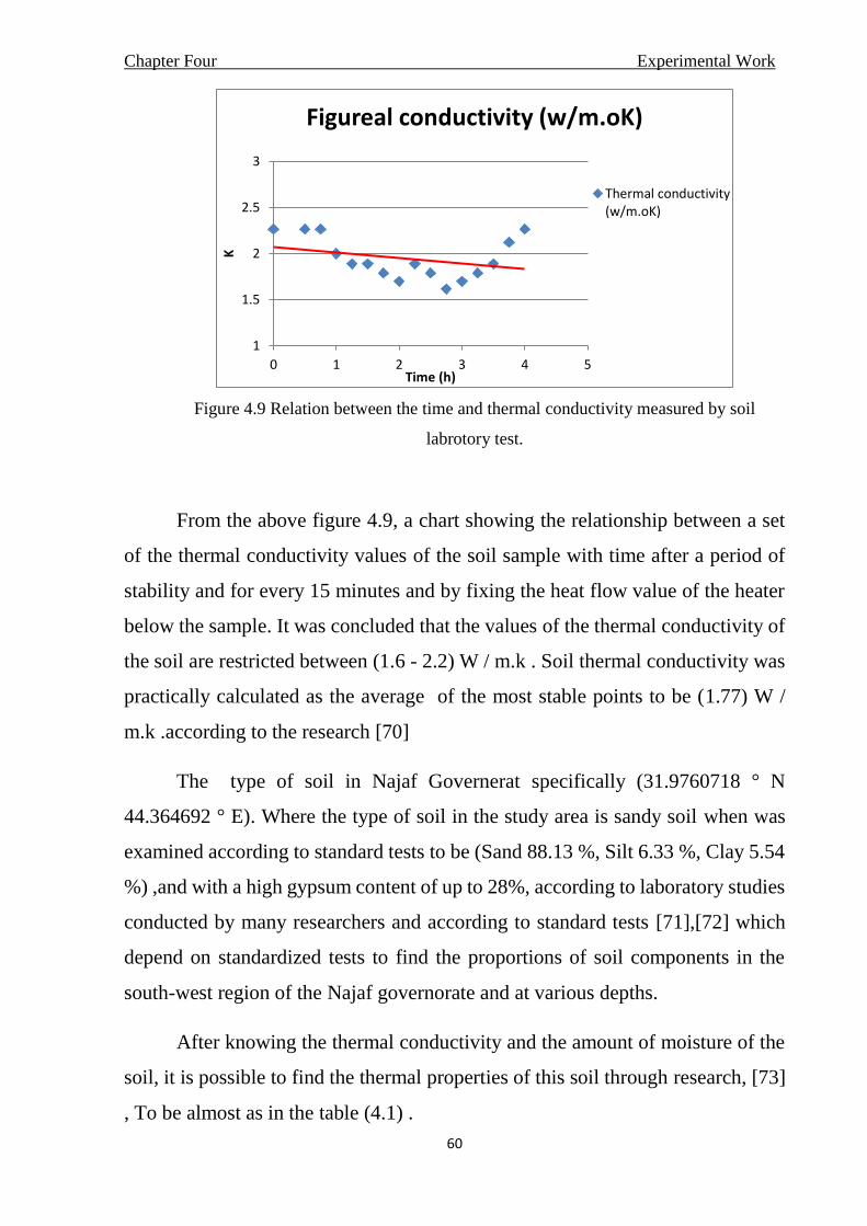
Chapter Four Experimental Work
60
Figure 4.9 Relation between the time and thermal conductivity measured by soil
labrotory test.
From the above figure 4.9, a chart showing the relationship between a set
of the thermal conductivity values of the soil sample with time after a period of
stability and for every 15 minutes and by fixing the heat flow value of the heater
below the sample. It was concluded that the values of the thermal conductivity of
the soil are restricted between (1.6 - 2.2) W / m.k . Soil thermal conductivity was
practically calculated as the average of the most stable points to be (1.77) W /
m.k .according to the research [70]
The type of soil in Najaf Governerat specifically (31.9760718 ° N
44.364692 ° E). Where the type of soil in the study area is sandy soil when was
examined according to standard tests to be (Sand 88.13 %, Silt 6.33 %, Clay 5.54
%) ,and with a high gypsum content of up to 28%, according to laboratory studies
conducted by many researchers and according to standard tests [71],[72] which
depend on standardized tests to find the proportions of soil components in the
south-west region of the Najaf governorate and at various depths.
After knowing the thermal conductivity and the amount of moisture of the
soil, it is possible to find the thermal properties of this soil through research, [73]
, To be almost as in the table (4.1) .
1
1.5
2
2.5
3
0 1 2 3 4 5
K
Time (h)
Figureal conductivity (w/m.oK)
Thermal conductivity(w/m.oK)

Chapter Four Experimental Work
61
Table (4.1) thermal properties of soil [73]
Depending on the thermal conductivity of the soil and the amount of
moisture measured experimentally and based on the researches, managed to
know the type of soil and the rest of its properties.
4.3.4 Setting sensors in the soil before burying the exchangers.
According to measures the temperature gradient of soil in the study area, it is
instilled 8 thermocouple type K sensor measure range (-50~350˚C), at each 0.5
m of grave depth, by setting the end of each sensor at along stick woodenly
perforated each half-meter so that the sensors touch the soil and from all sides,
to record the soil gradient temperature During a year in this region, as shown
in figure 4.10
Thermal properties of
soil
Conductivity
W/m.K
Dry density
kg/m3
Diffusivity
m2/day
Light sand (15% water) 1.0-2.1 1285 0.047-0.093
Figure 4.10 Setting the thermocuples to measuring the soil temperature gradient.

Chapter Four Experimental Work
62
4.3.5 Selecting the GHE piping type.
The type of piping used as shown in, figure 4.11 was chosen according to the
availability and the measurements calculated in the previous chapter, pipes were
chosen from the type of polyethylene multi-layer composite pipe (MLCP), this
type of pipes was used in most projects to benefit from geothermal energy directly
in modern systems. This is due to the advantages offered by this discovered type
of pipe.
Figure 4.11 Sectional view of pipe selected.
The advantage of MLCP pipes:
Light weight, flexible and form-stable.
Fast and fame free installation.
Low expansion rates, safety and clean.
No wastage and fewer fittings than traditional installations.
MLCP pipes have a life expectancy of minimum 50 years with correct use, and
it is not affected by the different soil components compared to the metal tubes.
Fully certified and approved across Europe.

Chapter Four Experimental Work
63
Table (4.2): properties and dimensions of selected piping system MLCP.
4.3.6 Forming the GHE
According to the available length, the MLCP pipes was divided and formed
as a two networks in a serpentine forms, each network with a length of 100 m, the
distance between pipes is 0.4 m, to bending the pipes a special tools was used, the
riser pipes which appears from the surface was isolated with good insulators to
maintain the temperature of the water coming out of the system constant. Shown
in figure 4.12 some tools used to fixing the pipes.
Figure 4.12 bending and pipe cutting tools with some accessories that used.
Inner diameter 0.012 m
Outer diameter 0.016 m
thickness 2 mm
thermal conductivity (kp) 0.040 W/m*ok
Endurance pressure 10 bar at 70 oC
Operating temperature ranges 0 oC to 95 oC
Minimal roughness 0.0004 mm
Expansion coefficient (α) 25 × 10-6(m/m ×o K)
Water volume 0.113 (l/m)
Roll Length 100 m

Chapter Four Experimental Work
64
The other step is to Install the first network by burying it at a depth of 3 m,
and implant a (1 meter) stick vertically, where it touched the beginning pipe
surface of the first network, to ensure the matching of the two layers as planned,
at M side view. then burying the second layer where the view of its pipes passes
through the mid-distance between the pipes of the first layer. The vertical distance
between the two layers is (0.5 m)(taking into account the distance between grains
and compressibility of sandy soil). this process is to make the pipes in a staggered
arrangement to reduce heat accumulation around the pipes, also to make the pipes
far from each other, to ensure the best heat transfer. The purpose of two layer
GHE used to decrease the area required to burying the heat exchanger (preserve
at long lengths of pipes with same efficient performance) as shown in figure 4.13,
figure 4.14 and figure 4.15 preparation of pipelines networks.
Figure 4.13 Burying the first serpentine networks at depth of 3m.
(The matching stick was removed after burying the second network)

Chapter Four Experimental Work
65
Figure 4.14 Matching the two layers of GHE.
Figure 4.15 Burying the second serpentine networks at depth 2.5m.
4.3.7 Final steps and external connections
To obtain an actual results the same soil was reused to burying the both
networks and thermocouples. Now the GHE became under the ground of the test
Matching stick
First layer
Second layer
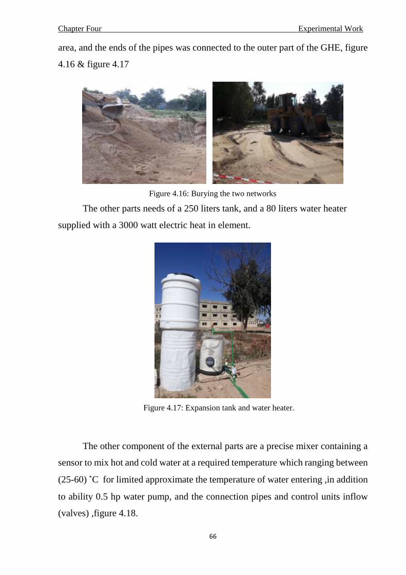
Chapter Four Experimental Work
66
area, and the ends of the pipes was connected to the outer part of the GHE, figure
4.16 & figure 4.17
Figure 4.16: Burying the two networks
The other parts needs of a 250 liters tank, and a 80 liters water heater
supplied with a 3000 watt electric heat in element.
Figure 4.17: Expansion tank and water heater.
The other component of the external parts are a precise mixer containing a
sensor to mix hot and cold water at a required temperature which ranging between
(25-60) ˚C for limited approximate the temperature of water entering ,in addition
to ability 0.5 hp water pump, and the connection pipes and control units inflow
(valves) ,figure 4.18.

Chapter Four Experimental Work
67
Figure 4.18 Mixer and water pump.
The control unit consists of a valve to control the flow rate, and an accurate
digital flowmeter (±1%) ,in addition to a distribution valve to control the
direction of water flow and distribute it into networks to study their
performance, together or individually as shown in figure 4.19. The entrance
and external end of the first and second networks pipes was marked with A1,
B1 and A2, B2 respectively.
Figure 4.19 Main components of control unit.
The data logger has four temperature sensors with accuracy ±0.5⁰ C, which
were connected to measure the water inlet and outlet temperature ((Tin,Tout) and
the ambient (Tatm) and soil surface temperature (Ts), as shown in Figure 4.20 .

Chapter Four Experimental Work
68
Figure 4.20: Data logger and its accessories.
Figure 4.21: Assembly of control unit.
So that the external devices and attachments are connected as shown in the
Figure 4.21
Other data logger with four channels, used thermocouples type K Used to
measure the soil temperature gradient at every half-meter depth, for 8 locations
on different depths of soil and over the course of the year 2019. As figure 4.22.
Figure 4.22: Data logger for Soil temperature gradient.

Chapter Four Experimental Work
69
4.4 EXPERIMENTAL WORK PROCEDURE:
At the beginning of any practical project of renewable energy or other
projects that are affected by weather conditions throughout the day or months of
the region in which the project is located, it is important to know the following:
4.4.1 Determine the appropriate times to record the readings.
In order to determine the appropriate time to measure the thermal gradient
of the soil from a depth of 3.5 m and for every 0.5 m to the soil surface during
each month and throughout the year 2019 for the region. It is necessary to know
the highest and the lowest temperature of weather that the region reaches during
the year, through the annual expectation of the temperature in Najaf governorate
(31.9760718°N 44.364692°E) for the year 2019, as shown in figure 4.23.
Figure 4.23: Average High and Low Temperature at Najaf in 2019 [74]
The above figure shows the maximum and minimum atmospheric
temperatures for the region according to the link of weather changes during the
year2019. Through it note the difference between temperatures during a year is
approximately 26.5 C (average between the highest and lowest temperature value
through day and night), which is equivalent to 2.21 C of change per month [74].

Chapter Four Experimental Work
70
For the purpose of obtaining a noticeable change .for that reason thermal
gradient readings of the soil were recorded experimental for every 15 days and
for a specific time during the day at 12:00 pm. And taking an average of the soil
temperature recorded during each month and from each season according to the
division of seasons in the figure 4.23, we obtain a figure 4.24 of the annual
gradient of the soil at different depths starting from the surface (shaded) to a depth
of 3.5 m and for every 0.5 m, where the relative stability of the soil temperature
results is clear between depths (2.5-3.5) m, during summer and winter seasons.
Figure 4.24: Soil temperature gradient of the test area.
The GHE operating time depends on its purpose, and because the project is
for the purpose of cooling test, it was self-evident that the working time in the
hottest months of this region where the ambient temperature naturally reach more
than 50oC, these months were determined by the annual thermal gradient of the
region's weather as it indicated in the Figure 4.23, which is from late April to mid-
September, The work was done and the results were recorded in June and part of
July from 2019.
-4
-3.5
-3
-2.5
-2
-1.5
-1
-0.5
0
0 10 20 30 40 50
De
pth
m
soil tempereture oC
Soil Temp. Gradient

Chapter Four Experimental Work
71
4.4.2 Practical procedures of GHE system.
The GHE, has been installed and connected as it indicated in figure 4.1. and
the sensors was set at the entrance and the exit of the inlet and outlet pipes, which
marked A1,A2, and B1, B2, for the first and second network respectively as figure
4.25. Then the system was operated experimentally for a period of time to bleed
the air from the network also to stabilize water flow inside pipes.
Figure 4.25 the inlet and outlet pipes mark in the system.
First, the performance of each network (layer of pipes) was tested
separately and their results were recorded. Then the performance of the two
networks (double-layers pipes) was tested together and their results were
recorded, to be compared later. Valves were placed at each entrance to the
network to control its closure and opening for separate and double testing with the
other network. Sediment-free water (R.O.) was used in the GHE system as a
circulating fluid and in a closed system. Three bands of flow were tested through
the main control valve placed in front of the water flow meter to determine the
measured flow values, where the flowrate values were determined after reviewing
a group of researchers and according to certain hypotheses. In addition, three
values of water temperature were tested. Inside and at every value of the flow.
Before recording any readings, the system must reach a steady-state, and this is
done by observing the stability of the temperature of the water entering the system,
A1 A2
B2 B1

Chapter Four Experimental Work
72
and after a certain period of time, where the temperature of the water entering
regulated, by the sensitive water mixer that regulated entered temperature value,
and monitored in the data logger screen through The sensor installed at the inlet
pipe. Taking into consideration the emptying of each layer of the water remaining
inside it from the previous experiment at each subsequent test.
Practical tests started in the summer season from June to July (12/6/2019 -
22/7/2019).
The first-layer was tested performance (the water inlet valve was closed to
the second-layer), which is at a depth of 3 m below the surface of the soil. The
water was circulated through 100 m of pipes with a different flow at (2-3-4)
ℓ/𝑚𝑖𝑛 with a change in the temperature of the water entering at each value of
flow to approximately between (30-60) ˚C, the temperature of entry (TA1) and
exit (TB1) was recorded(ambient temperature (Tamb) and soil surface temperature
(Ts) are also recorded for every half an hour and within 6 hours of the day (7:00
am-1:00 pm), for each amount of flow, as the first network experiments lasted 9
days (26/6/2019 - 8/7/2019(.
The second -layer was tested performance (the water inlet valve was closed
to the first-layer), which is at a depth of 2.5 m below the surface of the soil. In the
same way as the first network test, with the same flow rate, temperatures, and
time, the temperature of entry (TA2) and exit (TB2) was recorded (Ambient
temperature(Tamb) and soil surface temperature (Ts) are also recorded) for every
half an hour and within 6 hours of the day (7:00 am-1:00 pm), for each amount of
flow, as the second network experiments lasted 9 days also (12/6/2019 -
24/6/2019).
In the last, the double-layers (the water inlet valve of two layers opened
together) was tested performance. The water was circulated through 200 m of
pipes with a different flow at (3-4-5) ℓ/𝑚𝑖𝑛 with a change in the temperature of
the water entering at each value of flow to approximately between (30-60) ˚C, the

Chapter Four Experimental Work
73
temperature of entry (TA)and exit(TB) was recorded(Ambient
temperature(Tamb) and soil surface temperature (Ts) are also recorded) for every
half an hour and within 6 hours of the day (7:00 am-1:00 pm), for each amount of
flow, as the two networks experiments lasted 9 days also(10/7/2019 - 22/7/2019).
Figure 4.26 The readings of the flowmeter and Data logger are in
different circumstances
The results of the experiments were recorded and the amount of the lost
heat was found at each layer and for both layers together. The Figures were drawn
showing the difference in temperature degrees between entry and exit for each
layer and for the double-layers. after that, the comparison was made between
separate layer state and double-layers state after assume that when flowing
4 ℓ/𝑚𝑖𝑛 for the double-layer state the flow of each layer was 2 ℓ/𝑚𝑖𝑛 .
Considering that the flow is divided in half between the two layers because they
have the same diameter as the pipe. And as will be explained in Chapter Five.

Chapter Four Experimental Work
74

Chapter Five Results and Discussions
74
CHAPTER FIVE
RESULTS AND DISCUSSIONS
5.1 INTRODUCTION
In the introduction to this chapter, we test a ground heat exchanger
consisting of two layers of pipes, the length of each layer will be 100 meters, as a
measure to reduce the area used in horizontal geothermal heat exchangers in this
design, which is one of the problems of their use and reduce the cost in installing
horizontal geothermal heat exchangers with the same efficiency.
The practical results depend on the rotation of water (as the only fluid used in the
experiment) within the closed piping system to exploit the relative stability of the
soil temperature in the depths used and exclusively in the summer season to cool
the rotate fluid.
The temperature Δ𝑇 (The temperature difference between the water entering and
leaving the system pipes) and coefficient of performance COP )which equals the
amount of heat dissipated inside the soil over the work expended to circulate the
water) were used as the general performance to test the practical results of the
ground pipes system in addition to the soil gradient temperature. the experimental
data were set in tables and Figures as will be shown later in this chapter.

Chapter Five Results and Discussions
75
5.2 Ground Thermal Characteristics
The geothermal heat exchanger installed in space at the Technical College
of Engineering - Najaf southwest of the Najaf Governorate Center, which is
located in southwestern Iraq, specifically (31.9760718 ° N 44.364692 ° E). Where
the type of soil in the study area is light sandy soil.
The soil temperature varies according to the different weather conditions
during the months of the year, and the change is noticeable near the soil surface
and this change gradually decreases as go towards the depth to reach relative
stability at certain depths, and a noticeable change may also be recorded at the
surface of the soil due to the effect of air temperature on it during the day While
the change is almost non-existent at depths that reach the relative stability of the
temperature during day and night.
Results were recorded of the study area it was recorded soil temperature data at
different depths according to the thermocouples buried in the soil and at depths (0
- 0.5 -1 - 1.5 – 2 - 2.5 – 3 - 3.5) meters from the surface of the soil and record the
data through digital Datalogger, for every month for the year 2019(we record data
at 12:00pm ) Consequently, it made a summary of the results of the months
according to the seasons of the year.
Figure 5.1: Seasonal temperature Variation at different depths for soil
-4
-3.5
-3
-2.5
-2
-1.5
-1
-0.5
0
0 10 20 30 40 50
Dep
th (
m)
Temperature (°C)
summer
Autumn
winter
spring

Chapter Five Results and Discussions
76
Figure 5.1 shows the annual gradient of soil temperature and at different depths
of the study area, by taking the outcome of the recorded readings for each month
during the year 2019 and abbreviating it with four charts for the seasons of the y
Where it is noticed that the temperatures in the winter season at the surface are
lower than at the depths. Where that illustrate the nature of the annual temperature
gradient of the study soil.
While in the spring and autumn seasons the relative convergence of the
temperatures is observed at the different depths. while the summer scheme is
where the temperature of the soil surface reaches 40 degrees as an average for a
group of readings of the surface temperature The soil may reach higher values
during specific times, while the temperatures begin to decrease relatively
whenever we go to the specified depths, reaching approximately 25 degrees at a
depth of 3.5 meters below the surface of the soil. Which is considered a
comfortable temperature for humans.
Figure 5.2: Annual change of soil temperature at various depths.
0
5
10
15
20
25
30
35
40
45
50
0 2 4 6 8 10 12 14
Tem
per
atu
re
months
Depth 0m Depth 2.5m Depth 3m

Chapter Five Results and Discussions
77
In Figure 5.2, the effect of temperature changes on the soil surface according to
the change in the temperature of the atmosphere during the year 2019 with the
temperature of two different depths of the soil, in which the tuned pipe-layers
were installed at the two depths (2.5 &3) m in order to obtain a good heat
exchange During the year (better heat dissipation).due to the slight influence of
temperature and climatic conditions during the year at these depths for the study
area soil.
Figure 5.3: Temperature grid net with time
Figure 5.3 shows the temperature of the soil for the mentioned depths (2.5&3) m
with two charts for the temperature of the soil surface and the temperature of the
atmosphere surrounding the study area and during every hour of the day, and that
was on 1/6/2019. Where it becomes clear the relative stability of the temperature
of the depths in comparison with the temperature of the surrounding atmosphere
and the temperature of the surface of the soil affected by it.
5.3 Ground Heat Exchanger GHE
Due to the high temperatures in months of the year for the specified region,
and their rise to degrees approaching half the boiling degree in the summer, this
led to an increase in the consumption of refrigeration systems in addition to the
cost of installation and maintenance compared to the heating systems used.it had
15
20
25
30
35
40
45
50
Tem
per
atu
re
TimeTamb T0m T2.5m T3m

Chapter Five Results and Discussions
78
to search for alternative methods of cooling and test it. So headed to be the purpose
of the underground heat exchanger for cooling to contribute to finding a solution
to this problem, hence the work on testing the underground heat exchanger in the
hottest months of the year,(12/6/2019 -22/7/2019).
Figure 5.4: the average values of the intensity of solar radiation and the temperature of the
atmosphere over time at specific days in 2019
Figure 5.4 shows the average of a set of values of the intensity of solar radiation
with time, plus an average for a group of values of ambient temperature during
same time and date of recording the results for testing the underground heat
exchanger layers (first, second, and double layers state).
The ground heat exchanger consisting of two layers was tested for each layer
separately and then for the two layers together (in case of changing the flow rate
and the entry temperature of water into the ground heat exchanger). The following
are tables showing the results obtained in addition to the mathematical
calculations used.
Where the date and time appropriate for recording the results were recorded
in each table, as the system reached stability, and both the temperature of the
surrounding atmosphere and the surface of the soil and the temperature of the
water entering and leaving the piping layer by means of sensors placed and a data
100200300400500600700800900
39
40
41
42
43
44
45
Sola
r R
ad. (
W/m
²)
Time
Tam
p. (
˚C)
A relationship between both the intensity of solar radiation and the atmosphere temperature over time
Tamb. solar rad.

Chapter Five Results and Discussions
79
monitor. In addition to the calculation of the properties of water as being variable
with the water bulk temperature (Tb) (in the equation 3.26) and within certain
equations given in the appendix [63]. The velocity of flow(u) changes slightly
with the change in the water density, which is affected by the temperature at the
constant flow rate .Also, Prantel number and Nusselt number were calculated from
the equations mentioned in chapter three and find (h con. ) from them, which is
included in the calculation equation the fluid resistance equation (R con.), and
calculate the rest of the resistors (R total) to calculate the overall heat transfer
coefficient (U) which is included in the equation to calculate the rate of heat
transfer (Q).
The results were as follows:
5.3.1 First-layer GHE
The results of testing the first layer of the geothermal heat exchanger, which is at
a depth of 3 meters from the soil surface with length pipe 100m.
When we test the flow rate of 2 LPM (0.0333 kg/s) we get the results as in
the table below:
Table (5.1) Results of first-layer GHE at 2lpm flow
30/6/2019 27/6/2019 26/6/2019 Date
12:00 PM 10:00 AM 8:00 AM Time
53 44.9 38.1 T amb.
47.7 44 37.2 T soil
58.5 40.2 33.3 Tin
42.4 35.1 29.9 Tout
16.1 5.1 3.4 T
50.45 37.65 31.6 Tb
4181.24 4178.31 4178.51 Cp
987.72 993.05 995.14 ρ

Chapter Five Results and Discussions
80
0.2985 0.2969 0.2963 u
524.316 *E-6 667.355 *E-6 756.317 *E-6 µ
6748.933 5302.384 4623.669 Re
643.603 *E-3 626.957*E-3 618.007*E-3 K w
3.4063 4.4475 5.1741 Pr
38.4415 34.3353 32.2008 Nu
2061.752 1793.896 1658.361 h con.
0.012872 0.014794 0.016003 R con.
11.45 *E-3 11.45 *E-3 11.45 *E-3 R pipe
0.59556582 0.59556582 0.59556582 R soil
0.619890328 0.621812347 0.623021447 R total
0.321096453 0.320103946 0.319482719 U
0.126016301 0.1340214 0.139041346 P∆
2243.93 710.31 473.52 Q
358.6 358.6 358.6 Power
6.257474563 1.980795939 1.320479418 COP
After the system reached a state of stability every day and for the same flow,
the results of the entry temperature ranged between (30-60) ˚C and the exit
temperature, which was between (30-50) ˚C and noting the differences between
them, where the highest temperature difference was (16.1˚C) and higher. The rate
of heat transfer (2243.93 W) for this flow and the difference in the temperature of
the inlet water. This is due to the high temperature of the inlet water and the
difference between it and the initial soil temperature. In addition to measuring the
current consumed at this flow to be (1.63 A). The highest value (COP) (6.26) is
also recorded. Due to the higher temperature difference and the heat transfer rate
compared to the consumption rate.
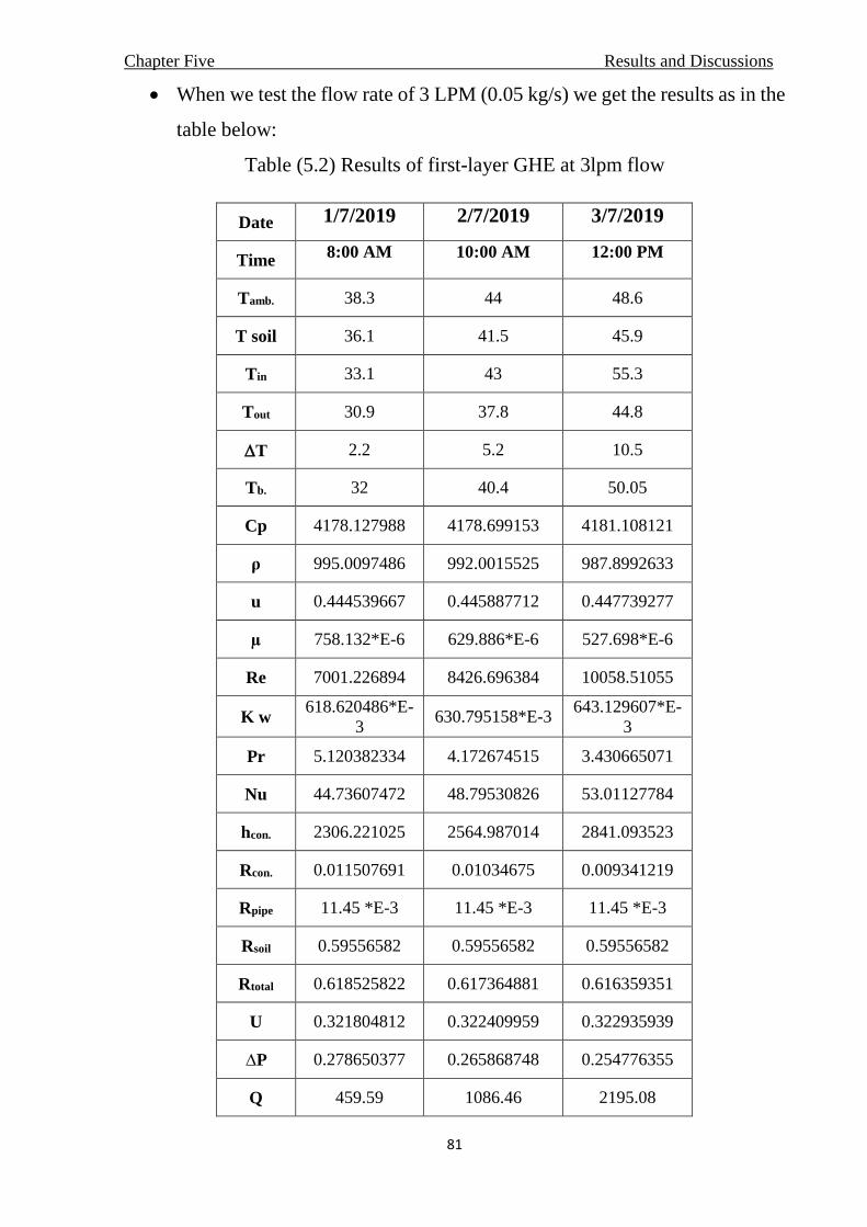
Chapter Five Results and Discussions
81
When we test the flow rate of 3 LPM (0.05 kg/s) we get the results as in the
table below:
Table (5.2) Results of first-layer GHE at 3lpm flow
3/7/2019 2/7/2019 1/7/2019 Date
12:00 PM 10:00 AM 8:00 AM Time
48.6 44 38.3 Tamb.
45.9 41.5 36.1 T soil
55.3 43 33.1 Tin
44.8 37.8 30.9 Tout
10.5 5.2 2.2 T
50.05 40.4 32 Tb.
4181.108121 4178.699153 4178.127988 Cp
987.8992633 992.0015525 995.0097486 ρ
0.447739277 0.445887712 0.444539667 u
527.698*E-6 629.886*E-6 758.132*E-6 µ
10058.51055 8426.696384 7001.226894 Re
643.129607*E-
3 630.795158*E-3
618.620486*E-
3 K w
3.430665071 4.172674515 5.120382334 Pr
53.01127784 48.79530826 44.73607472 Nu
2841.093523 2564.987014 2306.221025 hcon.
0.009341219 0.01034675 0.011507691 Rcon.
11.45 *E-3 11.45 *E-3 11.45 *E-3 Rpipe
0.59556582 0.59556582 0.59556582 Rsoil
0.616359351 0.617364881 0.618525822 Rtotal
0.322935939 0.322409959 0.321804812 U
0.254776355 0.265868748 0.278650377 P∆
2195.08 1086.46 459.59 Q

Chapter Five Results and Discussions
82
363 363 363 Power
6.047057199 2.993007658 1.26609939 COP
After the system reached a state of relative stability for every day, where the
entry temperature was recorded for the first, second, and third day to be roughly
between (30-60) ˚C and the exit temperature was roughly between (30-50) ˚C,
where the temperature gradient from low to medium then high during the three
days respectively. Noting the differences between them, where the highest
temperature difference was (10.5 ˚C) and higher. The rate of heat transfer
(2195.08W) for this flow and the difference in the temperature of the inlet water.
This is due to the high temperature of the inlet water and the difference between
it and the initial soil temperature. In addition to measuring the current consumed
at this flow to be (1.65 A). The highest value (COP) (6.05) is also recorded. Due
to the higher temperature difference and the heat transfer rate compared to the
consumption rate.
When we test the flow rate of 4 LPM (0.06667 kg/s) we get the results as
in the table below:
Table (5.3) Results of first-layer GHE at 4lpm flow
8/7/2019 7/7/2019 4/7/2019 Date
12:00 PM 10:00 AM 8:00 AM Time
49.5 43.6 35.7 Tamb.
43.1 38.4 34.6 Tsoil
50.9 42.8 32.9 Tin
42.7 38.1 30.6 Tout
8.2 4.7 2.3 T
46.8 40.45 31.75 Tb.
4180.140817 4178.707624 4178.142479 Cp

Chapter Five Results and Discussions
83
989.3516429 991.9819894 995.090321 ρ
0.596109321 0.594528673 0.592671563 u
557.505*E-6 629.242*E-6 762.61*E-6 µ
12694.30509 11247.08649 9280.156068 Re
639.1727*E-3 630.8636*E-3 618.2376*E-3 K w
3.646040973 4.167967325 5.153833264 Pr
65.0371415 61.45216043 56.1579401 Nu
3464.164227 3230.661028 2893.246011 hcon.
0.007661091 0.008214814 0.009172838 Rcon.
11.45 *E-3 11.45 *E-3 11.45 *E-3 Rpipe
0.59556 0.59556 0.59556 Rsoil
0.614679223 0.615232945 0.61619097 Rtotal
0.323818633 0.32352719 0.323024185 U
0.425906517 0.438168752 0.459278146 P∆
1560.64 1197.81 501.37 Q
367.4 367.4 367.4 Power
6.219770405 3.56376807 1.743735747 COP
As the system reaches stability when the entry temperature is low faster, while
the system needs more time to stabilize when the inlet water temperature rises, so
the results were recorded for different days and different times. Noting the
differences between them, where the highest temperature difference was (8.2 ˚C)
and higher. The rate of heat transfer (1560.64 W) for this flow and the difference
in the temperature of the inlet water .This is due to the high temperature of the
inlet water and the difference between it and the initial soil temperature. In
addition to measuring the current consumed at this flow to be (1.67 A). The
highest value (COP) (6.22) is also recorded. Due to the higher temperature
difference and the heat transfer rate compared to the consumption rate.

Chapter Five Results and Discussions
84
It is also noted from the tables above that the values of the heat transfer rate
converge upon increasing the flow with change in temperature different.
To more clearly demonstrate the changing effects on results with Figures, for
every half hour within six hours of the day ,we can divide them into:
The effect of temperature change at entry
Here are three Figures in each graph showing the difference between the entry
and exit temperature of the heat exchanger when the input temperature changes
to several values that are approximate to (30, 40, 50) ˚C and when stabilizing the
water flow values to ( 2,3,4) l/min.
Figure 5.5: the relationship between temperature difference and time when flowrate
2 ℓ/𝑚𝑖𝑛 and for the first-layer
Figure 5.5 shows that when the flow is constant at 2 l/min, we note that the
temperature change is in three patterns. The first is when the rate of the
temperature of entering the water is close to 30 ˚C, where the rate of change is
(3.48)˚C, and the second is when the rate of the temperature of the inlet water is
close to For 40 ˚C where the rate of change is recorded by (5.45)˚C. The highest
values of the outcome of the temperature difference (15.8) ˚C are recorded when
the inlet water is at a temperature close to 50 ˚C, due to the large difference
0
2
4
6
8
10
12
14
16
18
20
∆T
Time
at depth 3m (2lpm)
Tin ≈ 30°C Tin ≈ 40°C Tin ≈ 50°C
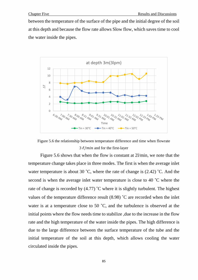
Chapter Five Results and Discussions
85
between the temperature of the surface of the pipe and the initial degree of the soil
at this depth and because the flow rate allows Slow flow, which saves time to cool
the water inside the pipes.
Figure 5.6 the relationship between temperature difference and time when flowrate
3 ℓ/𝑚𝑖𝑛 and for the first-layer
Figure 5.6 shows that when the flow is constant at 2l/min, we note that the
temperature change takes place in three modes. The first is when the average inlet
water temperature is about 30 ˚C, where the rate of change is (2.42) ˚C. And the
second is when the average inlet water temperature is close to 40 ˚C where the
rate of change is recorded by (4.77) ˚C where it is slightly turbulent. The highest
values of the temperature difference result (8.98) ˚C are recorded when the inlet
water is at a temperature close to 50 ˚C, and the turbulence is observed at the
initial points where the flow needs time to stabilize ,due to the increase in the flow
rate and the high temperature of the water inside the pipes. The high difference is
due to the large difference between the surface temperature of the tube and the
initial temperature of the soil at this depth, which allows cooling the water
circulated inside the pipes.
0
2
4
6
8
10
12
T
Time
at depth 3m(3lpm)
Tin ≈ 30°C Tin ≈ 40°C Tin ≈ 50°C

Chapter Five Results and Discussions
86
Figure 5.7: the relationship between temperature difference and time when flowrate
4 ℓ/𝑚𝑖𝑛 and for the first-layer
Figure 5.7 shows the temperature difference values of the circulating water
inside the pipes in three levels over time at the constant flow rate 4 l/min .Where
the first scheme is when the inlet temperature is close to 30 ° C, the difference is
little (1.92) ° C due to the slight difference between the temperature of the inlet
water and the soil surrounding the tube at that depth, while it begins to settle after
that, then is disturbed in the last hour due to the high temperature of the water
circulating inside the pipes. The second scheme, when the inlet temperature is
close to 40 ° C, where it is stable on the result of the temperature difference (4.92)
° C with little turbulence at the end due to the high temperature of the water
circulating While the third chart shows that when the entry temperature is close
to 50 ° C, with temperature difference (6.99) ° C the turbulence is clear at the
beginning due to the speed of the flow, while it takes stability, it returns to
turbulence slightly at the last hour due to the high temperature of the circulating
water and the change of its properties.
0
2
4
6
8
10
12
T
Time
at depth 3m(4lpm)
Tin ≈ 30°C Tin ≈ 40°C Tin ≈ 50°C

Chapter Five Results and Discussions
87
Flux effect
The following are chars that show the effect of changing the flow of water inside
the pipes at a temperature relatively of the water entering, through the amount of
heat transfer rate to the soil (in watt unit).
Where; q1, q2, q3 are heat transfer rate at temperature of the water entering is
approximate close to ≈30, 40 and 50C respectively.
Figure 5.8 the relationship between heat transfer rate and time when inlet water temperature
approximate 30C and for the first-layer
In Figure 5.8 above, when the incoming water temperature is
approximately 30 ° C, the average heat transfer rate is three plots at each flow
rate. The first diagram shows heat transfer values whose rate is (482.8 W) with
slight turbulence at constant flow (2 l/min) .While the randomness of the water
movement increases slightly when the flow increases to record the rate of heat
transfer (499.9W) at constant flow (3l/min). While the third chart shows the
turbulence about an hour (8:00AM) due to the increase in the flow to the
constant value (4l/min) so that the movement of water inside the pipelines will
be turbulent, as well as at about the clock (11:30). We notice the disturbance in
the values of the transmitted temperature due to the high temperature of the
200
300
400
500
600
700
800
Q(w
)
Time
at depth 3m (Tin ≈30C)
q1(2ɭpm) q2(3ɭpm) q3(4ɭpm)

Chapter Five Results and Discussions
88
water and the different properties of it, to record the rate of heat transfer
(555.7W).
Figure 5.9 the relationship between heat transfer rate and time when inlet water temperature
approximate 40C and for the first-layer
In the above Figure 5.9, when the incoming water temperature is
approximately 40˚C, the average heat transfer for the first chart when constant
flow rate at (2 l/min) it seems almost stable to be (755.4W).Whereas when the
constant flow values rise to (3 -4) l /min, it is noticed at the hour (8:00 AM) that
the values rise suddenly due to disturbance in the flow, while the values are in
contradiction before that. the scheme is at the flow (3 l/min) it is with high
values after that begins to decrease due to the low temperature of the inlet water
A little bit about it at the beginning, due to the surrounding conditions, to be
recorded as an outcome of values (983.6W). While the scheme at flow (4 l/min)
reaches the stability phase and then is slightly turbulent at the end due to the
high temperature of the circulating water to record an average of the sum of the
values of the heat transfer rate (1365.3 W).
400
600
800
1000
1200
1400
1600
1800Q
(w)
Time
at depth 3m (Tin≈ 40C)
q1(2ɭpm) q2(3ɭpm) q3(4ɭpm)

Chapter Five Results and Discussions
89
Figure 5.10: the relationship between heat transfer rate and time when inlet water
temperature approximate 50C and for the first-layer
In the above Figure 5.10, when the incoming water temperature is
approximately 50 ˚C, the average heat transfer rate in three charts for every value
of constant flowrate 2,3, and 4 l/min respectively. As it becomes clear that the
highest values of the heat transfer rate can be obtained, which is (2201.28W) when
the flow is (2l/min). While the turbulence in the values is clear when the flow (3
l/min) where it is oscillating between the lowest values of the start of the scheme,
but after an hour (10:00AM) begins to rise and converges from the values of the
temperature at the flow (2 l/min) to be recorded as an average (1874.8W) due to
the high temperature of the inlet water, and the difference between it and the
temperature of the soil increases At that depth and increased flow rate also affect
turbulence. observe the large fluctuation of the values of the heat transfer rate
when increasing the flow to (4 l/min), where random values ranging from the
highest and lowest values are recorded so that their rate is (1935.97 W) the
stability is between hours (11:00am-12:00pm) and the fluctuation is due to the
high temperature of the inlet water, which causes its properties to change and
increases the randomness of the flow with Increase the flow rate at this layer.
1000
1200
1400
1600
1800
2000
2200
2400
2600
2800
Q(w
)
Time
at depth 3m ( ≈50C)
q1(2ɭpm) q2(3ɭpm) q3(4ɭpm)

Chapter Five Results and Discussions
90
The effect of performance coefficient (COP) of GHE
The following are three charts that show the relationship between the performance
coefficient values of the first stratum with time according to the difference in
temperature difference values between the incoming and outgoing water for each
diagram, and with constant flow rates 2, 3, and 4 l/min.
Figure 5.11:COP values with time at inlet temperature approximate 30 ˚C and at three
constant flow rates.
In figure 5.11, we note the convergence of the performance parameter
values according to the difference in flow when the inlet temperature is close to
30 ° C. The average of values at flow (2 l/min) is (1.35), while (1.38) at flow (3
l/min). At the flow (4 l/min) it is noticed that the values are lower at the start. and
began slightly be high to be the average values of the performance factor (1.4),
due to the proportionality between the temperature difference and the rate of flow,
to the electrical consumption.
0
0.5
1
1.5
2
2.5
3
7:00AM
7:30AM
8:00AM
8:30AM
9:00AM
9:30AM
10:00AM
10:30AM
11:00AM
11:30AM
12:00PM
12:30PM
1:00PM
CO
P
Time
Cop values at Tin ≈30˚C
COP(2lpm) COP(3lpm) COP(4lpm)

Chapter Five Results and Discussions
91
Figure 5.12 COP values with time at inlet temperature approximate 40 ˚C and at three
constant flow rates.
In figure 5.12, three plots of the performance parameter values of the
system are shown with time at each constant flow rate value, and when the inlet
water temperature is approximately 40 ° C. The average of values at flow (2 l/min)
is (2.1). Whereas when the flow rate is (3 l/min), the beginning of the scheme is a
few values due to the increase in flow, then it starts to rise at the hour (8:00 am),
the highest value is recorded, then the relative stability begins. For circulating
water at this flow, the resulting values are (2.75). The third chart is at the constant
flow value (4 l/min), where it records the highest values of the performance
parameter despite the disturbance occurring at the beginning and end of the
scheme and is at a rate (3.75) due to the direct proportion between the increase in
flow and the amount of heat dissipation in addition to the temperature difference
values and the rate of electricity consumption at this flow.
1.5
2
2.5
3
3.5
4
4.5
5
7:00AM
7:30AM
8:00AM
8:30AM
9:00AM
9:30AM
10:00AM
10:30AM
11:00AM
11:30AM
12:00PM
12:30PM
1:00PM
CO
P
Time
Cop values at Tin ≈40˚C
COP(2lpm) COP(3lpm) COP(4lpm)

Chapter Five Results and Discussions
92
Figure 5.13 COP values with time at inlet temperature approximate 50 ˚C and at three
constant flow rates.
In figure 5.13, three plots of the performance parameter values of the
system are shown with time at each constant flow rate value, and when the inlet
water temperature is approximately 50 ° C. Notice the turbulence and instability
of the charts until the hour (8:30 am). Record the average values of the
performance parameter (5.9) at the flow (2 l/min). While at the flow (3 l/min) with
alternating values that are few at the beginning of the scheme, it starts to rise at
the hour (10:30 am) to be its rate (5.2) due to the availability of more time for heat
exchange at this flow. While the chart at the flow (4 l/min) is turbulent at the
beginning, it reaches the stability phase between the hours (9:00-11:30) am to
record an average of (5.25) values less than the rest of the flow values due to the
lack of time for heat exchange for the speed of the flow of water in addition to the
amount of electrical consumption greater at this amount of flow.
3
4
5
6
7
8
7:00AM
7:30AM
8:00AM
8:30AM
9:00AM
9:30AM
10:00AM
10:30AM
11:00AM
11:30AM
12:00PM
12:30PM
1:00PM
CO
P
Time
COP values at Tin≈50˚C
COP(2lpm) COP(3lpm) COP(4lpm)

Chapter Five Results and Discussions
93
5.3.2 Second-Layer GHE
The results of testing the second layer of the geothermal heat exchanger, which is
at a depth of 2.5 meters from the soil surface. Length of pipes 100 m.
When we test the flow rate of 2 LPM (0.0333 kg/s) we get the results as in
the table below:
Table (5.4) Results of second-layer GHE at 2lpm flow
16/6/2019 13/6/2019 12/6/2019 Date
12:00 PM 10:00 AM 8:00 AM Time
43.6 39.6 33.6 Tamb.
40.4 37.2 32.8 Tsoil
53.4 41.8 29.6 Tin
39.8 31.1 26.6 Tout
13.6 5.7 3 T
46.6 36.45 28.1 Tb.
4180.085997 4178.200705 4178.625189 Cp
989.4387501 993.4867822 996.2029043 ρ
0.298028421 0.296814083 0.296004827 u
559.481*E-6 685.029*E-6 832.784*E-6 µ
6324.73212 5165.577989 4249.086402 Re
638.922*E-3 625.236*E-3 612.513*E-3 K w
3.660349679 4.577766531 5.681334696 Pr
37.29222687 33.91712767 30.95276128 Nu
1985.570988 1767.186553 1579.914102 hcon.
0.013366069 0.015017814 0.016797925 Rcon.
11.45
*E-3
11.45
*E-3
11.45
*E-3 Rpipe
0.590615748 0.590615748 0.590615748 Rsoil
0.603981816 0.605633561 0.607413673 Rtotal
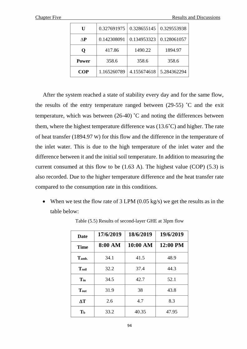
Chapter Five Results and Discussions
94
0.329553938 0.328655145 0.327691975 U
0.128061057 0.134953323 0.142308091 P∆
1894.97 1490.22 417.86 Q
358.6 358.6 358.6 Power
5.284362294 4.155674618 1.165260789 COP
After the system reached a state of stability every day and for the same flow,
the results of the entry temperature ranged between (29-55) ˚C and the exit
temperature, which was between (26-40) ˚C and noting the differences between
them, where the highest temperature difference was (13.6˚C) and higher. The rate
of heat transfer (1894.97 W) for this flow and the difference in the temperature of
the inlet water. This is due to the high temperature of the inlet water and the
difference between it and the initial soil temperature. In addition to measuring the
current consumed at this flow to be (1.63 A). The highest value (COP) (5.3) is
also recorded. Due to the higher temperature difference and the heat transfer rate
compared to the consumption rate in this conditions.
When we test the flow rate of 3 LPM (0.05 kg/s) we get the results as in the
table below:
Table (5.5) Results of second-layer GHE at 3lpm flow
19/6/2019 18/6/2019 17/6/2019 Date
12:00 PM 10:00 AM 8:00 AM Time
48.9 41.5 34.1 Tamb.
44.3 37.4 32.2 Tsoil
52.1 42.7 34.5 Tin
43.8 38 31.9 Tout
8.3 4.7 2.6 T
47.95 40.35 33.2 Tb

Chapter Five Results and Discussions
95
4180.466884 4178.690732 4178.087957 Cp
988.845614 992.021097 994.6154611 ρ
0.447310779 0.445878927 0.444715892 u
546.469*E-6 630.531*E-6 737.202*E-6 µ
9712.998764 8418.077978 7200.001391 Re
640.595*E-3 630.726*E-3 620.441*E-3 K w
3.566206384 4.177391763 4.96435859 Pr
52.15217733 48.77190884 45.32656871 Nu
2784.038784 2563.478552 2343.540984 hcon.
0.009532654 0.010352838 0.011324435 Rcon.
11.45
*E-3
11.45
*E-3
11.45
*E-3 Rpipe
0.57916 0.57916 0.579163436 Rsoil
0.600148402 0.600968586 0.601940183 Rtotal
0.331658945 0.331206307 0.330671704 U
0.256874431 0.265936121 0.276644912 P∆
1734.89 981.99 543.15 Q
363 363 363 Power
4.779321644 2.705213008 1.496284943 COP
After the system reached a state of relative stability for every day, where the
entry temperature was recorded for the first, second, and third day to be roughly
between (30-53) ˚C and the exit temperature was roughly between (30-45) ˚C,
where the temperature gradient from low to medium then high during the three
days respectively. Noting the differences between them, where the highest
temperature difference was (8.3 ˚C) and higher. The rate of heat transfer (1734.9
W) for this flow and the difference in the temperature of the inlet water. This is
due to the high temperature of the inlet water and the difference between it and
the initial soil temperature. In addition to measuring the current consumed at this

Chapter Five Results and Discussions
96
flow to be (1.65 A). The highest value (COP) (4.78) is also recorded. Due to the
higher temperature difference and the heat transfer rate compared to the
consumption rate.
When we test the flow rate of 4 LPM (0.06667 kg/s) we get the results as
in the table below:
Table (5.6) Results of second-layer GHE at 4lpm flow
24/6/2019 23/6/2019 20/6/2019 Date
12:00 PM 10:00 AM 8:00 AM Time
46.3 42 34.6 Tamb.
39.9 38.5 33.5 Tsoil
50.3 43 35 Tin
44.3 38.9 32.9 Tout
6 4.1 2.1 T
47.3 40.95 33.95 Tb.
4180.280334 4178.795034 4178.086559 Cp
989.1327071 991.7853378 994.3627832 ρ
0.596241265 0.594646557 0.593105199 u
552.639*E-6 622.878*E-6 724.586*E-6 µ
12806.0845 11361.99729 9767.146777 Re
639.794*E-3 631.545*E-3 621.566*E-3 K w
3.610824123 4.121444883 4.870575543 Pr
65.30445768 61.74565897 57.51963116 Nu
3481.786426 3249.600062 2979.354081 hcon.
0.007622317 0.008166937 0.008907729 Rcon.
11.45
*E-3
11.45
*E-3
11.45
*E-3 Rpipe
0.57916 0.57916 0.57916 Rsoil
0.598238064 0.598782685 0.599523477 Rtotal

Chapter Five Results and Discussions
97
0.332718023 0.332415401 0.332004657 U
0.425051185 0.437107563 0.453469725 P∆
1672.11 1142.20 584.93 Q
367.4 367.4 367.4 Power
4.551203412 3.108883985 1.592085243 COP
As the system reaches stability when the entry temperature is low faster,
while the system needs more time to stabilize when the inlet water temperature
rises, so the results were recorded for different days and different times. Noting
the differences between them, where the highest temperature difference was (6
˚C) and higher. The rate of heat transfer (1672 W) for this flow and the difference
in the temperature of the inlet water. This is due to the high temperature of the
inlet water and the difference between it and the initial soil temperature. In
addition to measuring the current consumed at this flow to be (1.67 A). The
highest value (COP) (4.55) is also recorded. Due to the higher temperature
difference and the heat transfer rate compared to the consumption rate.
It is also noted from the tables above that the values of the heat transfer rate
converge upon increasing the flow with a change in temperature difference for
water circulating in pipes of second-layer at depth 2.5 m from the surface.in
addition that results are less than of the first-layer because of the temperature of
the soil in this depth and weather conditions at the surrounding in thes dates.
To more clearly demonstrate the changing effects on results with Figures,
for every half hour within six hours of the day ,we can divide them into:

Chapter Five Results and Discussions
98
The effect of temperature change at entry
Here are three Figures in each graph showing the difference between the entry
and exit temperature of the heat exchanger when the input temperature changes
to several values that are approximate to (30, 40, 50) ˚C and when stabilizing the
water flow values to ( 2,3,4) l/min.
Figure 5.14: the relationship between temperature difference and time when flowrate
2 ℓ/𝑚𝑖𝑛 and for the second-layer
In the above Figure 5. 14 when the flow is constant at 2l/min, notice that
the temperature change is in three patterns. The first is when the rate of the
temperature of entering the water is close to 30 ˚C, where the rate of change is
(3.32)˚C, and the second is when the rate of the temperature of the inlet water is
close to For 40 ˚C where the rate of change is recorded by (5.72)˚C.at the
beginning of the first and second schemes ,the values are almost equal due to the
instability of the system in this point .The highest values of the outcome of the
temperature difference (13.41) ˚C are recorded when the inlet water is at a
temperature close to 50 ˚C, due to the large difference between the temperature of
the surface of the pipe and the initial degree of the soil at this depth and because
the flow rate allows Slow flow, which saves time to cool the water inside the
pipes.
0
2
4
6
8
10
12
14
16
T
Time
at depth 2.5m(2lpm)
Tin ≈ 30°C Tin ≈ 40°C Tin ≈ 50°C

Chapter Five Results and Discussions
99
Figure 5.15: the relationship between temperature difference and time when flowrate
3 ℓ/𝑚𝑖𝑛 and for the second-layer
In the above Figure 5. 15 shows that when the flow is constant at 2l/min,
we note that the temperature change takes place in three modes. The first is when
the average inlet water temperature is about 30 ˚C, where the rate of change is
(2.6) ˚C. And the second is when the average inlet water temperature is close to
40 C where the rate of change is recorded by (4.7) C where it is slightly turbulent.
The highest values of the temperature difference result (8.3) C are recorded when
the inlet water is at a temperature close to 50 ˚C, due to the increase in the flow
rate and the high temperature of the water inside the pipes. The high difference is
due to the large difference between the surface temperature of the tube and the
initial temperature of the soil at this depth, which allows cooling the water
circulated inside the second-layer of pipes.
0
1
2
3
4
5
6
7
8
9
10
T
Time
at depth 2.5m(3lpm)
Tin ≈ 30°C Tin ≈ 40°C Tin ≈ 50°C
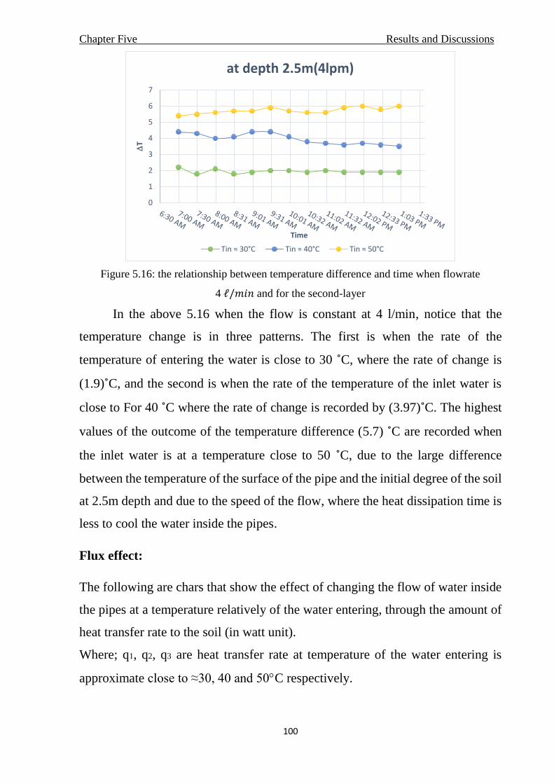
Chapter Five Results and Discussions
100
Figure 5.16: the relationship between temperature difference and time when flowrate
4 ℓ/𝑚𝑖𝑛 and for the second-layer
In the above 5.16 when the flow is constant at 4 l/min, notice that the
temperature change is in three patterns. The first is when the rate of the
temperature of entering the water is close to 30 ˚C, where the rate of change is
(1.9)˚C, and the second is when the rate of the temperature of the inlet water is
close to For 40 ˚C where the rate of change is recorded by (3.97)˚C. The highest
values of the outcome of the temperature difference (5.7) ˚C are recorded when
the inlet water is at a temperature close to 50 ˚C, due to the large difference
between the temperature of the surface of the pipe and the initial degree of the soil
at 2.5m depth and due to the speed of the flow, where the heat dissipation time is
less to cool the water inside the pipes.
Flux effect:
The following are chars that show the effect of changing the flow of water inside
the pipes at a temperature relatively of the water entering, through the amount of
heat transfer rate to the soil (in watt unit).
Where; q1, q2, q3 are heat transfer rate at temperature of the water entering is
approximate close to ≈30, 40 and 50C respectively.
0
1
2
3
4
5
6
7
T
Time
at depth 2.5m(4lpm)
Tin ≈ 30°C Tin ≈ 40°C Tin ≈ 50°C
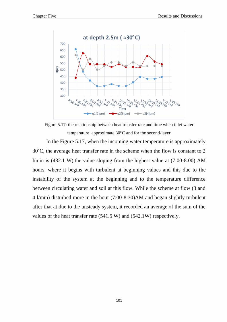
Chapter Five Results and Discussions
101
Figure 5.17: the relationship between heat transfer rate and time when inlet water
temperature approximate 30C and for the second-layer
In the Figure 5.17, when the incoming water temperature is approximately
30˚C, the average heat transfer rate in the scheme when the flow is constant to 2
l/min is (432.1 W).the value sloping from the highest value at (7:00-8:00) AM
hours, where it begins with turbulent at beginning values and this due to the
instability of the system at the beginning and to the temperature difference
between circulating water and soil at this flow. While the scheme at flow (3 and
4 l/min) disturbed more in the hour (7:00-8:30)AM and began slightly turbulent
after that at due to the unsteady system, it recorded an average of the sum of the
values of the heat transfer rate (541.5 W) and (542.1W) respectively.
300
350
400
450
500
550
600
650
700
Q(w
)
Time
at depth 2.5m ( ≈30C)
q1(2ɭpm) q2(3ɭpm) q3(4ɭpm)
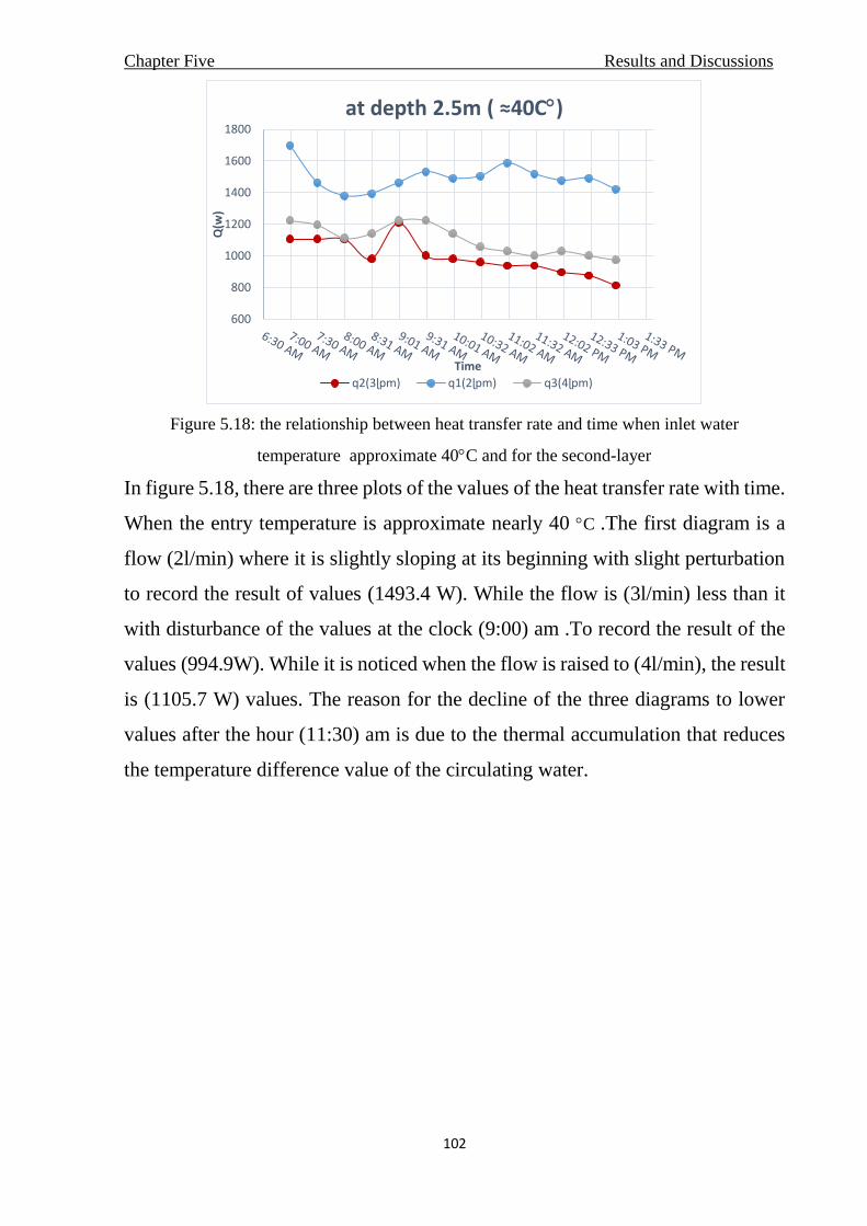
Chapter Five Results and Discussions
102
Figure 5.18: the relationship between heat transfer rate and time when inlet water
temperature approximate 40C and for the second-layer
In figure 5.18, there are three plots of the values of the heat transfer rate with time.
When the entry temperature is approximate nearly 40 C .The first diagram is a
flow (2l/min) where it is slightly sloping at its beginning with slight perturbation
to record the result of values (1493.4 W). While the flow is (3l/min) less than it
with disturbance of the values at the clock (9:00) am .To record the result of the
values (994.9W). While it is noticed when the flow is raised to (4l/min), the result
is (1105.7 W) values. The reason for the decline of the three diagrams to lower
values after the hour (11:30) am is due to the thermal accumulation that reduces
the temperature difference value of the circulating water.
600
800
1000
1200
1400
1600
1800
Q(w
)
Time
at depth 2.5m ( ≈40C)
q2(3ɭpm) q1(2ɭpm) q3(4ɭpm)

Chapter Five Results and Discussions
103
Figure 5.19: the relationship between heat transfer rate and time when inlet water
temperature approximate 50C and for the second-layer
In Figure 5.19, there are three heat transfer rate plots over time. When the entry
temperature is approximate nearly 50 C .The first plot is flow (2 l/min) where
there is a slight disturbance to record the result of values (1868.1 W). While the
flow (3l/min) from it with disturbance in the values to record the result of the
values (1734.8 W), where the highest value is recorded at the beginning due to
instability, while the value decreases after an hour (1:00)pm due to the decrease
in the temperature difference. While it is observed when the flux is raised to
(4l/min), the average of the values is (1594.9 W) with little turbulence. The
cause of thermal accumulation reduces the value of the temperature difference
of circulating water.
The effect of performance coefficient (COP) of GHE
The following are three charts that show the relationship between the performance
coefficient values of the second stratum with time according to the difference in
temperature difference values between the incoming and outgoing water for each
diagram, and with constant flow rates 2, 3, and 4 l/min.
1300
1400
1500
1600
1700
1800
1900
2000
Q(w
)
Time
at depth 2.5m ( ≈50C)
q1(2ɭpm) q2(3ɭpm) q3(4ɭpm)

Chapter Five Results and Discussions
104
Figure 5.20: COP values with time at inlet temperature approximate 30 ˚C and at three
constant flow rates.
In figure 5.20, there are three diagrams for the performance parameter values,
which differ at each constant value of the flow, and at the inlet water temperature
approximately close to 30 ° C. Records different values for the charts at an hour
(7:00)am due to the instability of the system. Record the sum of the values of
(1.49) and (1.47) at flow (3l/min) and (4l/min) respectively. While the decreases
slightly at flowrate (2l/min) to be recorded as a rate (1.25) due to the slow flow of
water at this flow.
0
0.5
1
1.5
2
2.5
3
7:00AM
7:30AM
8:00AM
8:30AM
9:00AM
9:30AM
10:00AM
10:30AM
11:00AM
11:30AM
12:00PM
12:30PM
1:00PM
CO
P
Time
Cop values at Tin ≈30˚C
COP(2lpm) COP(3lpm) COP(4lpm)
Figure 5.21 COP values with time at inlet temperature approximate 30 ˚C and at three
constant flow rates.
1.5
2
2.5
3
3.5
4
4.5
5
7:00AM
7:30AM
8:00AM
8:30AM
9:00AM
9:30AM
10:00AM
10:30AM
11:00AM
11:30AM
12:00PM
12:30PM
1:00PM
CO
P
Time
Cop values at Tin ≈40˚C
COP(2lpm) COP(3lpm) COP(4lpm)

Chapter Five Results and Discussions
105
In figure 5.21, there are three diagrams for the performance parameter values,
which differ at each constant value of the flow, and at the inlet water temperature
approximately close to 40 ° C. Note when flowing (2l/min) the highest average
values recorded, which (4.2) . While it is noted when flowing (3l/min), a
disturbance is recorded at an hour (9:00) am, to be recorded as the average values
(2.7). When the flow (4l/min), the rate of the performance parameter (3) is
recorded. It is noted that the values of the two diagrams are decreased at the runoff
(3l/min) and (4l/min) due to the lower temperature difference of the incoming and
outgoing water.
Figure 5.22 COP values with time at inlet temperature approximate 30 ˚C and at three
constant flow rates.
3
3.5
4
4.5
5
5.5
6
7:00AM
7:30AM
8:00AM
8:30AM
9:00AM
9:30AM
10:00AM
10:30AM
11:00AM
11:30AM
12:00PM
12:30PM
1:00PM
CO
P
Time
Cop values at Tin ≈50˚C
COP(2lpm) COP(3lpm) COP(4lpm)

Chapter Five Results and Discussions
106
In figure 5.22, there are three diagrams for the performance parameter values,
which differ at each constant value of the flow, and at the inlet water temperature
approximately close to 50 ° C. Record the highest values of the performance
parameter at flow (2l/min) to be (5.2). Following the chart at flow comes (3l/min)
to be (4.78). While the lowest values are recorded at flow (4l/min) to be the
average values of performance coefficient (4.3). This is due to the increase in the
rate of electricity consumption with the increase in flow.
5.3.3 Double-Layers GHE
The results of the two-layer test together for the ground heat exchanger at depth
2.5m and 3m.when length of pipes become 200m. When operating the system as
two layers together, the increase in the length of the pipes allows more time for
heat exchange, as the flow rate is less than it is in the single-layer separately, so
the flow rates 3, 4, and 5 l/min were taken for testing according to the hypothesis
of equations explained in the appendix.
When we test the flow rate of 3 LPM (0.05 kg/s) we get the results as in the
table below:
Table (5.7) Results of double-layers GHE at 3lpm flow
14/7/2019 11/7/2019 10/7/2019 Date
12:00 PM 10:00 AM 8:00 AM Time
47.8 45.4 38.9 Tamb.
44.3 42 37.3 Tsoil
53.1 44.1 34.3 Tin
36.6 33.6 29.7 Tout
16.5 10.5 4.6 T
44.85 38.85 32 Tb
4179.631227 4178.461966 4178.127988 Cp
990.189402 992.598689 995.0097486 ρ

Chapter Five Results and Discussions
107
0.446703733 0.44561947 0.444539667 u
577.521*E-6 650.496*E-6 758.132*E-6 µ
9190.751574 8159.702035 7001.226894 Re
636.70253*E-
3
628.6493*E-
3
618.6204*E-
3 K w
3.791136919 4.32367253 5.120382334 Pr
50.82056613 48.0643545 44.73607472 Nu
2696.465218 2517.968713 2306.221025 hcon.
0.009842248 0.010539955 0.011507691 Rcon.
11.45
*E-3
11.45
*E-3
11.45
*E-3 Rpipe
0.59556582 0.59556582 0.59556582 Rsoil
0.616860379 0.617558087 0.618525822 Rtotal
0.161336822 0.161154546 0.160902406 U
0.520574292 0.536011618 0.557300754 P∆
3448.20 2193.69 960.97 Q
363 363 363 Power
9.499161879 6.043230117 2.647298725 COP
After operating the two layers together at the aforementioned flow, it is
possible to reach a steady-state in a short time when the inlet water temperature is
approximately close to 30 ° C. While it takes more time for the entry of water at
a temperature close to 40 ° C. And it takes more time to reach stability due to the
high temperature of the inlet water to about 50 ° C. When the inlet water
temperature is between (30-55) ° C during the three days, the outgoing water
temperature is between (29-37) ° C when climatic conditions are for the days in
which the results are recorded and the aforementioned time. Where we notice the
highest temperature difference (16.5)° C, which was obtained when the inlet water
temperature was high due to the large difference between the temperature of the
piping surface and the soil at the depths (2.5&3)m in addition to slow flow
velocity which provides time for heat dissipation. After finding the set of results

Chapter Five Results and Discussions
108
and recording them in the above table, we notice that the highest value of the heat
transfer rate is recorded (3448.2 W) due to the high-temperature difference. While
the highest value of the performance coefficient of the double-layer system is
recorded to be (9.49), due to the lack of current consumed (1.65 A) at the
aforementioned flow, in addition to the value of the high heat transfer rate
obtained, which is approximately (1 ton refrigeration).
When we test the flow rate of 4 LPM (0.06667 kg/s) we get the results as
in the table below:
Table (5.8) Results of double-layers GHE at 4lpm flow
17/7/2019 16/7/2019 15/7/2019 Date
12:00 PM 10:00 AM 8:00 AM Time
48.9 47 41 Tamb.
45.8 43.9 38.5 Tsoil
50.5 45.2 33.3 Tin
38.5 35.3 30.3 Tout
12 7.9 3 T
44.5 40.25 31.8 Tb
4179.545828 4178.674038 4178.139406 Cp
990.3370166 992.06013 995.0742502 ρ
0.595516199 0.594481845 0.592681135 u
581.295*E-6 631.824*E-6 761.711*E-6 µ
12174.79101 11201.12203 9291.107088 Re
636.2515*E-3 630.589*E-3 618.314*E-3 K w
3.818533374 4.186856506 5.147116609 Pr
63.77728469 61.33430972 56.1889622 Nu
3381.532792 3223.064254 2895.20324 hcon.

Chapter Five Results and Discussions
109
0.007848298 0.008234176 0.009166637 Rcon.
11.45*E-3 11.45*E-3 11.45*E-3 Rpipe
0.59556582 0.59556582 0.59556582 Rsoil
0.61486643 0.615252308 0.616184769 Rtotal
0.161860021 0.161758504 0.161513718 U
0.860091339 0.87719571 0.918285286 P∆
3343.64 2757.92 835.63 Q
367.4 367.4 367.4 Power
9.100807465 7.506600068 2.274436258 COP
After operating the two layers together at the aforementioned flow, it is
possible to reach a steady-state in a short time when the inlet water temperature is
approximately close to 30 ° C. While it takes more time for the entry of water at
a temperature close to 40 ° C. And it takes more time to reach stability due to the
high temperature of the inlet water to about 50 ° C. When the inlet water
temperature is between (30-51) ° C during the three days, the outgoing water
temperature is between (30-40) ° C when climatic conditions are for the days in
which the results are recorded and the aforementioned time. Where we notice the
highest temperature difference (12)° C, which was obtained when the inlet water
temperature was high due to the large difference between the temperature of the
piping surface and the soil at the depths (2.5&3)m in addition to flow velocity
which provides time for heat dissipation. After finding the set of results and
recording them in the above table, we notice that the highest value of the heat
transfer rate is recorded (3343.6 W) due to the high-temperature difference. While
the highest value of the performance coefficient of the double-layer system is
recorded to be (9.1), due to the current consumed (1.67 A) at the aforementioned
flow, in addition to the value of the high heat transfer rate obtained.
When we test the flow rate of 5 LPM (0.08333 kg/s) we get the results as
in the table below:
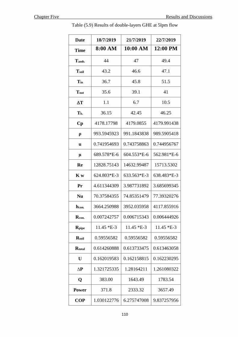
Chapter Five Results and Discussions
110
Table (5.9) Results of double-layers GHE at 5lpm flow
22/7/2019 21/7/2019 18/7/2019 Date
12:00 PM 10:00 AM 8:00 AM Time
49.4 47 44 Tamb.
47.1 46.6 43.2 Tsoil
51.5 45.8 36.7 Tin
41 39.1 35.6 Tout
10.5 6.7 1.1 T
46.25 42.45 36.15 Tb.
4179.991438 4179.0855 4178.17798 Cp
989.5905418 991.1843838 993.5945923 ρ
0.744956767 0.743758863 0.741954693 u
562.981*E-6 604.553*E-6 689.578*E-6 µ
15713.5302 14632.99487 12828.75143 Re
638.483*E-3 633.563*E-3 624.803*E-3 K w
3.685699345 3.987731892 4.611344309 Pr
77.39320276 74.85351479 70.37584355 Nu
4117.855916 3952.035958 3664.250988 hcon.
0.006444926 0.006715343 0.007242757 Rcon.
11.45 *E-3 11.45 *E-3 11.45 *E-3 Rpipe
0.59556582 0.59556582 0.59556582 Rsoil
0.613463058 0.613733475 0.614260888 Rtotal
0.162230295 0.162158815 0.162019583 U
1.261080322 1.28164211 1.321725335 P∆
1783.54 1643.49 383.00 Q
3657.49 2333.32 371.8 Power
9.837257956 6.275747008 1.030122776 COP

Chapter Five Results and Discussions
111
After operating the two layers together at the aforementioned flow, it is
possible to reach a steady-state in a short time when the inlet water temperature is
approximately close to 30 ° C. While it takes more time for the entry of water at
a temperature close to 40 ° C. And it takes more time to reach stability due to the
high temperature of the inlet water to about 50 ° C. When the inlet water
temperature is between (35-52) ° C during the three days, the outgoing water
temperature is between (35-42) ° C when climatic conditions are for the days in
which the results are recorded and the aforementioned time. Where we notice the
highest temperature difference (10.5)° C, which was obtained when the inlet water
temperature was high due to the large difference between the temperature of the
piping surface and the soil at the depths (2.5&3)m. After finding the set of results
and recording them in the above table, we notice that the highest value of the heat
transfer rate is recorded (3657.49 W) which is approximately (1 ton
refrigeration).due to the temperature difference and high value of flow rate. While
the highest value of the performance coefficient of the double-layer system is
recorded to be (9.8), due to the current consumed (1.69 A) at the aforementioned
flow, in addition to the value of the high heat transfer rate obtained.
To more clearly demonstrate the changing effects on results with Figures, for
every half hour within six hours of the day ,we can divide them into:
The effect of temperature change at entry
Here are three Figures in each graph showing the difference between the entry
and exit temperature of the heat exchanger when the input temperature changes
to several values that are close to 30, 40 and 50C and when stabilizing the water
flow values to different values.

Chapter Five Results and Discussions
112
Figure 5.23: the relationship between temperature difference and time when flowrate
3 ℓ/𝑚𝑖𝑛 and for the double-layers
In the above Figure 5.23 when the flow is constant at 3l/min, Note that the rate of
change in temperature 4.1, 11.22, and 15.9 C for the inlet water temperature
values approximate approaching 30, 40, and 50C respectively, at steady flow
(3l/min). Due to slow flow rate and availability of exchange time in addition to
the large difference between the inlet water temperature and the initial soil
temperature at depths (3&2.5) meters
0
2
4
6
8
10
12
14
16
18
T
Time
at depth 2.5m&3m(3lpm)
Tin ≈ 30°C Tin ≈ 40°C Tin ≈ 50°C

Chapter Five Results and Discussions
113
Figure 5.24: the relationship between temperature difference and time when flowrate
4 ℓ/𝑚𝑖𝑛 and for the double-layers
In the Figure 5.24 when the flow is constant at 4 l/min, notice that the
temperature change is in three patterns. The first is when the rate of the
temperature of entering the water is close to 30 ˚C, where the rate of change is
(3.29)˚C, and the second is when the rate of the temperature of the inlet water is
close to For 40 ˚C where the rate of change is recorded by (8.32)˚C. The highest
values of the outcome of the temperature difference (11.2) ˚C are recorded when
the inlet water is at a temperature close to 50 ˚C, due to the large difference
between the temperature of the surface of the pipe and the initial degree of the soil
at 2.5&3m depths and due to the speed of the flow, where the heat dissipation the
water inside the pipes.
0
2
4
6
8
10
12
14
T
Time
at depth 2.5m&3m(4lpm)
Tin ≈ 30°C Tin ≈ 40°C Tin ≈ 50°C

Chapter Five Results and Discussions
114
Figure 5.25: the relationship between temperature difference and time when flowrate
5 ℓ/𝑚𝑖𝑛 and for the double-layers
In the Figure 5.25, Notice that the rate of change in temperature from high to low
1.4, 6.3 and 10 C for the approximate inlet water temperature values approaches
30, 40 and 50, respectively, at steady flow (5l/min). Because of the speed of flow
at the rate of flow and the lack of time for heat exchange in addition to the large
difference between the temperature of the inlet water and the initial soil
temperature at depths of (2.5&3) meters for high temperatures. After the piping
system reached to stay-state.
Flux effect
The following are chars that show the effect of changing the flow of water
inside the pipes at a temperature relatively of the water entering, through the
amount of heat transfer rate to the soil (in watt unit).
Where; q1, q2, q3 are heat transfer rate at temperature of the water entering is
approximate close to ≈30, 40 and 50˚C respectively.
0
2
4
6
8
10
12
T
Time
at depth 2.5m&3m(5lpm)
Tin ≈ 30°C Tin ≈ 40°C Tin ≈ 50°C

Chapter Five Results and Discussions
115
Figure 5.26: the relationship between heat transfer rate and time when inlet water
temperature approximate 30C and for the double-layers
In Figure 5.26 shows charts at an entry temperature close to 30 ° C. The first plot
is at flow (3l/min), where it descends from the highest values at the hour (7:00am)
to the lowest value at the hour (10:00)am, after which it begins to rise .the average
become (854.9 W). This disturbance in the plot is due to dividing the flow into
two networks, and The high difference temperature of the soil at the depths is
compared with the temperature of the inlet water. As for the scheme at the flow
(4l/min), the beginning of the scheme is with turbulent values due to the lack of
stability until the hour (8:30) am to record (910.6 W). While the scheme at the
flow (5l/min) is graduated from a few values at the beginning, it was started by
stabilizing to record the result (487.5 W) due to the high flow, which does not
provide sufficient time for heat dissipation.
0
200
400
600
800
1000
1200
1400
Q(w
)
Time
at depth 2.5&3m ( ≈30C)
q1(3ɭpm) q2(4ɭpm) q3(5ɭpm)
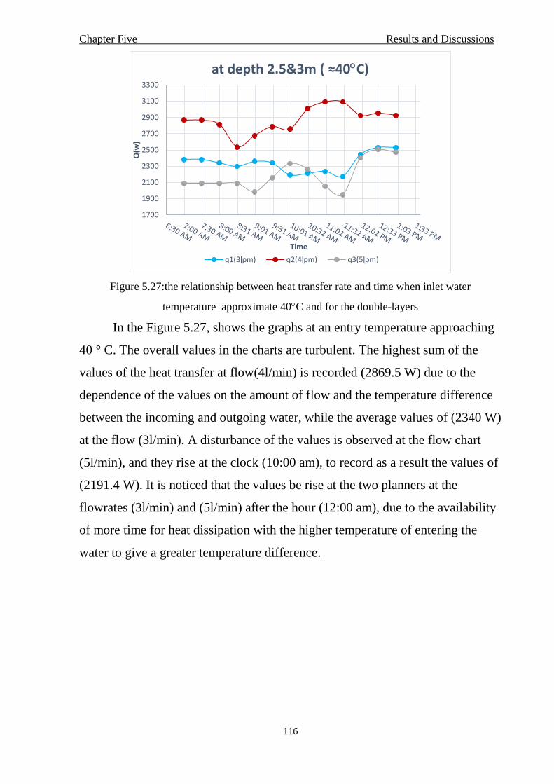
Chapter Five Results and Discussions
116
Figure 5.27:the relationship between heat transfer rate and time when inlet water
temperature approximate 40C and for the double-layers
In the Figure 5.27, shows the graphs at an entry temperature approaching
40 ° C. The overall values in the charts are turbulent. The highest sum of the
values of the heat transfer at flow(4l/min) is recorded (2869.5 W) due to the
dependence of the values on the amount of flow and the temperature difference
between the incoming and outgoing water, while the average values of (2340 W)
at the flow (3l/min). A disturbance of the values is observed at the flow chart
(5l/min), and they rise at the clock (10:00 am), to record as a result the values of
(2191.4 W). It is noticed that the values be rise at the two planners at the
flowrates (3l/min) and (5l/min) after the hour (12:00 am), due to the availability
of more time for heat dissipation with the higher temperature of entering the
water to give a greater temperature difference.
1700
1900
2100
2300
2500
2700
2900
3100
3300
Q(w
)
Time
at depth 2.5&3m ( ≈40C)
q1(3ɭpm) q2(4ɭpm) q3(5ɭpm)

Chapter Five Results and Discussions
117
Figure 5.28 the relationship between heat transfer rate and time when inlet water
temperature approximate 50C and for the double-layers
In the Figure 5.28, when the inlet water temperature rises to about 50 C
or slightly higher or slightly lower. shows charts at each flow and notes the
highest rate of heat transfer values that are (3485.7W) at flow (5l/min) due to the
direct mathematical proportion between the amount of flow and the heat
transferred, with the observation of turbulence and the rise of the values after
The time (11:30) am, due to the increase in the temperature of the circulating
water. While the diagram at constant flow (3l/min) records the average values of
(3337.1 W) due to the slow flow velocity which saves time for heat dissipation.
Whereas the scheme records when the flow (4l/min) average values of (3109.9
W) gradually increase due to the increase in the temperature difference with the
increase in the temperature of the circulating water inside the two layers.
2500
2700
2900
3100
3300
3500
3700
3900
Q(w
)
Time
at depth 2.5&3m ( ≈50C)
q1(3ɭpm) q2(4ɭpm) q3(5ɭpm)

Chapter Five Results and Discussions
118
The effect of performance coefficient (COP)of GHE:
The following are three charts that show the relationship between the performance
coefficient values of the two stratum with time according to the difference in
temperature difference values between the incoming and outgoing water for each
diagram, and with constant flow rates 2, 3, and 4 l/min.
Figure 5.29 COP values with time at inlet temperature approximate 30 ˚C and at three
constant flow rates.
In Figure 5.29, three plots of the performance parameter values are shown
in two layers with time . in which the plot at flow (4l/min) records the highest
result of the values reaching (2.48), followed by the scheme at flow (3l/min),
where the average values of (2.36) are recorded. It is also noticed that the previous
two charts start with high values due to instability, after which the values
converge, while the lowest values of the performance coefficient of the system
are recorded at the flow (5l/min) the amount of (1.3), due to the high flow, which
increases the electricity consumption compared with the temperature difference
of the circulating water inside the system.
0
1
2
3
4
5
7:00AM
7:30AM
8:00AM
8:30AM
9:00AM
9:30AM
10:00AM
10:30AM
11:00AM
11:30AM
12:00PM
12:30PM
1:00PM
CO
P
Time
COP values at Tin≈30˚C
COP(3lpm) COP(4lpm) COP(5lpm)

Chapter Five Results and Discussions
119
Figure 5.30 COP values with time at inlet temperature approximate 40 ˚C and at three
constant flow rates.
In Figure 5.30, three charts of the performance of coefficient values are
shown in two layers with time at water entered temperature approximate close to
40˚C. in which the chart at flow (4l/min) records the highest result of the values
reaching (7.8), followed by the scheme at flow (3l/min), where the average values
of (6.4) are recorded. While the lowest values of the performance coefficient of
the system are recorded at the flow (5l/min) to be (5.9), due to the high flow,
which increases the electricity consumption compared with the temperature
difference of the circulating water inside the system. With noticing the
disturbance in charts due to divided water flow inside two layers of pipes.
4
5
6
7
8
9
10
7:00AM
7:30AM
8:00AM
8:30AM
9:00AM
9:30AM
10:00AM
10:30AM
11:00AM
11:30AM
12:00PM
12:30PM
1:00PM
CO
P
Time
COP values at Tin≈40˚C
COP(3lpm) COP(4lpm) COP(5lpm)

Chapter Five Results and Discussions
120
Figure 5.31 COP values with time at inlet temperature approximate 50 ˚C and at three
constant flow rates.
In Figure 5.31, three charts of the performance of coefficient values are
shown in two layers with time. When the temperature of water entered is close to
50˚C. A slight slope of the values until the hour (9:00) am is observed in the chart
when flowing (5l/min), after which the values are disturbed, and then the chart
begins to rise to register as a rate (9.4), while the values are disturbed up and down
in the chart when the flow (3l/min) is recorded as the average (9.1). While the
lowest values of the rate are (8.6) where the flow (4l/min). It is noticed that the
performance coefficient is high after the hour (12:00 pm) due to the high
temperature and the accompanying rise in the difference between the temperature
of entering and exiting the water inside the system.
7
7.5
8
8.5
9
9.5
10
10.5
11
7:00AM
7:30AM
8:00AM
8:30AM
9:00AM
9:30AM
10:00AM
10:30AM
11:00AM
11:30AM
12:00PM
12:30PM
1:00PM
CO
P
Time
COP values at Tin≈50˚C
COP(3lpm) COP(4lpm) COP(5lpm)

Chapter Five Results and Discussions
121
5.4 A comparison between the results of the layers of the pipes of
GHEs To compare the results of the two layers of pipes separately with the results
of the two layers of pipes together, their results were taken at two joint flow rate
between them where the water was entered with the flow of 2 l/min for each layer
separately and be 4 l/min as a total flow rate for both layers as well, with a change
in the temperature of the water entering at each flow For approximately 30,40 and
50 ˚C.
The difference can be seen in the values of each heat transfer rate (Q) for
every layer and for two-layers.
Where; the first-layer GHE can be represented by the number 1
Second-layer GHE can be represented by the number 2
The double-layers GHE can be represented by the number 3
Figure 5.32: a comparison of the heat transfer rate with time for each layer separately and
for double- layers at inlet temperature approximate 30C.
The Figure 5.32 shows the values of the heat transfer rate when the
temperature of entering water approximately 30C degrees, in the two-layer chart,
the value of heat transfer rate at the beginning be high and stoop upon hour (8:00
am)to record highest the average value (910.7W) compared with each separate
0
200
400
600
800
1000
1200
Q(W
)
Time
At Tin ≈ 30˚C
Q1 (3m) Q2 (2.5 m) Q3 (3&2.5)m

Chapter Five Results and Discussions
122
layer . While the first and second layer recording the convergent average values
(482.9 W) and (432.1 W) respectively, at same conditions, due high flowrate and
effect on the rate of the heat transfer value
Figure 5.33: a comparison of the heat transfer rate with time for each layer separately and
for double- layers at inlet temperature approximate 40C.
The Figure 5.33 shows the values of the heat transfer rate when the
temperature of entering water approximately 40C degrees, Where the two layers
recorded together with the highest value, reaching an average of (2869.47 W),
after which the second layer recorded a rate of (1493.4 W) due to the moisture of
the soil at the depth (2.5m) in the test day, then the first layer recorded a rate of
heat transfer of (755.39 W).
0
500
1000
1500
2000
2500
3000
3500
Q(W
)
Time
At T in ≈ 40˚C
Q1 3m Q2 2.5 m Q3 3&2.5

Chapter Five Results and Discussions
123
Figure 5.34 a comparison of the heat transfer rate with time for each layer separately and
for double- layers at inlet temperature approximate 50C.
The Figure 5.34 shows the values of the heat transfer rate when the
incoming water temperature of approximately 50C, Where the two layers were
recorded together with the highest value reaching the average (3109.9 W), while
the heat transfer rate values were (2201.3 W) and (1868.1W) for the first and
second mesh, respectively. Due to the high flow rate of the two layers together,
which increases the value of the dissipated heat rate from water inside pipes to
soil.
The comparison can also be noticed when testing the same values of flow
and temperature of the incoming water for the two layers together and then for
each layer separately through the performance of the coefficient of the pipes layer,
as in the following diagrams:
1000
1500
2000
2500
3000
3500
4000
Q(W
)
Time
At Tin ≈ 50˚C
Q1 3m Q2 2.5 m Q3 3&2.5

Chapter Five Results and Discussions
124
The Figure 5.35 shows an illustration of three charts of the performance
coefficient values the highest COP values at the lowest in the case of double
layers and at each layer separately during a specified time when the inlet water
temperature is approximately 30 ° C. Where the average values of the
performance coefficient values of the two layers together have the highest values
reaching (2.48) due to the increase in the amount of circulating water and the
increase in the length of the pipes, which allows for better heat dissipation
compared to the separate layers. Where the first and second grid recorded rates
(1.35) and (1.26) respectively. A disturbance in the values is observed at the
beginning of the charts due to time of the steady-state.
Figure 5.35comparison COP values with time at inlet temperature approximate 30 ˚C for
each layer separate and with double-layers.
0
0.5
1
1.5
2
2.5
3
3.5
7:00AM
7:30AM
8:00AM
8:30AM
9:00AM
9:30AM
10:00AM
10:30AM
11:00AM
11:30AM
12:00PM
12:30PM
1:00PM
CO
P
Time
COP values at T in ≈30˚C & flowrate 2 lpm
COP1 COP2 COP3

Chapter Five Results and Discussions
125
Figure 5.36: comparison COP values with time at inlet temperature approximate 40 ˚C for
each layer separate and with double-layers.
Figure 5.37comparison COP values with time at inlet temperature approximate 50 ˚C for
each layer separate and with double-layers.
In Figure 5.36 an illustration of three charts of the performance coefficient
values in the case of double layers and at each layer separately during a specified
time when the inlet water temperature is approximately 40 ° C. Where the average
values of the performance coefficient values of the two layers together have the
highest values reaching (7.82) due to the increase in the amount of circulating
water and the increase in the length of the pipes, which allows for better heat
0123456789
7:00AM
7:30AM
8:00AM
8:30AM
9:00AM
9:30AM
10:00AM
10:30AM
11:00AM
11:30AM
12:00PM
12:30PM
1:00PM
CO
P
Time
COP values at T in ≈40˚C & flowrate 2 lpm
COP1 COP2 COP3
0
2
4
6
8
10
12
7:00AM
7:30AM
8:00AM
8:30AM
9:00AM
9:30AM
10:00AM
10:30AM
11:00AM
11:30AM
12:00PM
12:30PM
1:00PM
CO
P
Time
COP values at T in ≈50˚C & flowrate 2 lpm
COP1 COP2 COP3

Chapter Five Results and Discussions
126
dissipation compared to the separate layers. Where the first and second grid
recorded rates (2.14) and (4.16) respectively. Due to the moisture of the soil at the
depth (2.5m) in the test day.
While the Figure 5.37 shows the three diagrams, where a disturbance and
difference in the initial values is observed due to the time of the system to reach
a stable state. Where the highest values of the average performance coefficient are
recorded at both layers (8.59). While the values of the first and second layers are
close to each other due to the convergence of temperature at these depths, to
record (5.9) and (5.2) as the average values of their performance coefficient
respectively. Because of the increase in the flow rate of the two layers together
compared with the separate layers.

Chapter six Conclusions and Recommendations
127
CHAPTER SIX
CONCLUSIONS AND RECOMMENDATIONS
6.1 Conclusions
Conclude from the results recorded in the previous chapter the following:
1) With regard to thermal sensors for soils with the aforementioned
characteristics in the previous chapter, and for the different depths that gradient
at every half meter from the surface of the earth, down to a depth of 3.5 meters.
Notice the large effect with a temperature of atmosphere and weather
conditions, to the surface soil temperature, and it was observed with and this
effect gradually decreases with increasing depth. The average annual
temperature was for two depths (2.5 m) and (3 m) are (22.2˚C) and (22.1˚C)
respectively.
2) The relative stability of the temperature at specific depths during the seasons
of the year and its stability during the hour of day at a certain temperature with
a noticeable change in the ambient temperature.
3) It describes the performance of GHE in a two-layer case better than piping
system due to the increase in the length of the tube and the division of the flow
rate within the two clusters to achieve a slow speed in the flow of water
circulating inside the closed system, which saves time for better dissipating the
water temperature through the soil.

Chapter six Conclusions and Recommendations
128
4) The higher the temperature of the water entering the system, the higher the
temperature difference between entering and exiting the circulating water
inside the pipes. This is to increase the difference between the temperature of
the surface of the tube and the temperature of the soil at the specified depths
(which is characterized by the relative stability of the temperature with
different weather conditions).
5) The lower the water flow rate inside the pipes decreased the velocity of the
water. which leads the higher the difference in temperature of the circulating
water due to the availability of time for heat exchange between the tube surface
and the soil, and vice versa.
6) When testing the first piping layer that is located at a depth of (3m), the highest
rate of heat transfer (2410.58W) is recorded at the temperature difference
(17.3) ˚C and by constant flow (2 l/min). This was in the hour (7:30) am of the
date (30/6/2019). While the second layer, which is located at a depth of (2.5
m) when tested separately, recorded the highest heat transfer rate (1922.7W)
at the temperature difference (13.8) ˚C and constant flow (2 l/min). This was
in the hour (10:00) pm of the date (16/6/2019). Whereas the rate of heat
transfer is approximately one refrigeration ton when the two layers are tested
together to record (3531.89W) at the temperature difference (16.9) C and with
the constant flow (3 l/min) in the hour (12:30) pm from the date
(14/7/2019).Because of the direct proportionality of the heat transfer rate with
both the temperature difference of the circulating water and the amount of
flow.
7) he highest performance coefficient values (COP) for the first layer, second
layer, and two-layers heat exchanger are 5.9,5.2 and 8.58 respectively, at the
same conditions. According to the rate of increased flow, which leads to a little
increase in electricity consumption, to the values of the heat transfer rate
recorded that affect directly on performance coefficient values.
Chapter six Conclusions and Recommendations
129
6.2 Recommendations for future works
1. A large difference can be obtained for transferring heat when misleading
the area or plant planting, where increasing the moisture increases the thermal
conductivity of the soil.
2. Heat transfer can be increasing in the soil around the tubes by mixing them
with components that improve the heat transfer properties of the surrounding soil.
3. The circulating water inside the pipes can be replaced with another fluid
and compare the performance of the underground exchanger. )fluid with a freezing
factor above zero(
4. The two-layer heat exchanger can be operated alternately to avoid thermal
accumulation in the soil around the tubes which occurs over time.
5. It is possible to make the underground heat exchanger as open system and
compare the performance of the exchanger.
6. The heat exchanger can be tested in the case of drawing heat from the soil
to warm the fluid circulating inside the pipes and test its performance in the winter
season.
7. In addition to the proposal to design a heat pump to take advantage of the
transfer of heat to and from the soil to use the system to cool and heat rooms.
8. The system can be tested by introducing water at high temperatures above
50˚ C and with flow values less than 2 l/min to achieve a greater difference in
temperature degrees, which increases the rate of heat transfer to the system.

References

References
References
[1] .Banerjee, R. (2015). Importance of Energy Conservation. International
Journal of Innovatice Research in Advanced Engineering, 2(4), 186–190.
[2]. https://www.bbc.com/timelines/zqgxtfr
[3]. https://quranenc.com/ar/browse/english_saheeh/16
[4]. Santamouris M., Mihalakaha G., Balaras C.A., Argirioua A.D. and
Vallinaras M., Use of buried pipes for energy conservation in cooling of
agricultural greenhouse, Solar Energy, 35, 111 (1995 .)
[5]. Zhu, J., Hu, K., Lu, X., Huang, X., Liu, K., & Wu, X. (2015). A review of
geothermal energy resources, development, and applications in China:
Current status and prospects. Energy, 93(December), 466–483.
https://doi.org/10.1016/j.energy.2015.08.098
[6].Doeff, M. M. (2012). Encyclopedia of Sustainability Science and Technology
- Battery Cathode Materials, (January 2012). https://doi.org/10.1007/978-1-
4419-0851-3
[7]. Miller, C. C. (2006). Chapter two. Forbes (Vol. 178).
[8]. Florides, G., & Kalogirou, S. (2007). Ground heat exchangers-A review of
systems, models and applications. Renewable Energy, 32.
https://doi.org/10.1016/j.renene.2006.12.014
[9].Alghannam, A. (2012). "Investigations of performance of earth tube heat
exchanger of sandy soil in hot arid climate." Journal of Applied Sciences
Research(June): 3044-3052".
[10]. Yusof, T., et al. (2015). "A review of ground heat exchangers for cooling
application in the Malaysian climate." Journal of Mechanical Engineering
and Sciences: 1426-1439.
[11] Muntadher M. Ali, Dhafer Manea Hachim, Hassanain Hammed, “Numerical
Investigation for Single Slope Solar Still Performance with Optimal Amount
of Nano-PCM”, Journal of Advanced Research in Fluid Mechanics and
Thermal Sciences Vol. 63, Issue 2, pp. 302-316, 2019.

References
[12] Hiba Q.Mohammed, Ali Sh. Baqir, Hasan S.Khwayyir, " Effects of Air
Bubble Injection on the Efficiency of a Flat Plate Solar Collector: An
Experimental Study for the Open Flow System" Journal of Engineering and
Applied Sciences, Vol. 15 No. 7, pp. 1703-1708
[13] Hasan S.Khwayyir, Ali Sh. Baqir, Hiba Q.Mohammed, “Effect of Air
Bubble Injection on the Thermal Performance of a Flat Plate Solar
Collector”, Thermal Science and Engineering progress,
https://doi.org/10.1016/j.tsep.2019.100476.
[14] Hassanain Hammed, Hayder Aziz Neema, “Experimental Study for
Productivity Enhancement of a Parabolic Solar Concentrator System”,
AlQadisiya Journal for Engineering sciences, Vol. 4, No. 2, pp 37-41, 2011.
[15] Hassanain Hammed, Ahmed H. Ali, Zaid M. Al-Dulaimi,
“EXPERIMENTAL INVESTIGATION OF THE ENHANCEMENT
PARAMETERS ON THE PERFORMANCE OF SINGLE-SLOPE SOLAR
STILL”, nternational Journal of Latest Trends in Engineering and
Technology Vol.(10)Issue(3), pp.139-145
[16] Dhafer Manea. H. Al-Shamkhi, “Experimental Study of the Performance of
Low Cost Solar Water Heater in Najaf City”, International Journal of
Mechanical & Mechatronics Engineering IJMME-IJENS, Vol. 16, Issue 1,
pp. 109-121, 2018.
[17] Ali Sh. Baqir, Hameed B. mahood, “Optimisation and evaluation of NTU
and effectiveness of a helical coil tube heat exchanger with air injection”,
Thermal Science and Engineering Progress Volume 14, December 2019
[18] Nawfel M. Baqer, Ali Shakir Baqir, “Numerical Investigation for
Enhancement of Heat Transfer in Internally Finned Tubes Using
ANSYSCFX Program, “
[19] Ali Majeed Abed AL –Kreem, Ahmad Hashim Yousif, Ali Shakir Baqir,
“Study the effect of twisted tapes on thermal performance solar collector
with using curvature vortex generators,” Technology of Kansai University,
Volume 62, Issue 07, PP. 3631-3643,2020.

References
[20] Basil N. Merzha, Majid H. Majeed, Fouad A. Saleh, Experimental study of
flat plate solar collector performance with twisted heat pipe, IOP Conference
Series: Materials Science and Engineering 518 (3), 032035 (2019)
[21] Basil N. Merzha, Majid H. Majeed, and Fouad A. Saleh, Numerical study of
flat plate solar collector performance with square shape wicked evaporator,
Al-Qadisiyah Journal for Engineering Sciences 12 (2), 90-97. (2019)
[22]. Kharseh, M. and L. Altorkmany (2012). "How global warming and building
envelope will change buildings energy use in central Europe." Applied
energy 97: 999-1004.
[23]. Kharseh, M., et al. (2015). "Analysis of the effect of global climate change
on ground source heat pump systems in different climate categories."
Renewable Energy 78: 219-225.
[24]. Sivasakthivel, T., et al. (2015). "Study of technical, economical and
environmental viability of ground source heat pump system for Himalayan
cities of India." Renewable and Sustainable Energy Reviews 48: 452-462
[25].Esen, H., et al. (2007). "A techno-economic comparison of ground-coupled
and air-coupled heat pump system for space cooling." Building and
environment 42(5): 1955-1965.
[26].Demir, H., et al. (2009). "Heat transfer of horizontal parallel pipe ground heat
exchanger and experimental verification." Applied Thermal Engineering
29(2-3): 224-233.
[27]. Eicker, U. and C. Vorschulze (2009). "Potential of geothermal heat
exchangers for office building climatisation." Renewable Energy 34(4):
1126-1133.
[28]. Shua'a, A. K. M. and N. S. Sabeeh (2009). Analysis The Performance of
Underground Heat Exchanger. Second Scientific Conference of the College
of Engineering, University of Al-Qadisiya
[29]. Ozgener, L. and O. Ozgener (2010). "An experimental study of the exergetic
performance of an underground air tunnel system for greenhouse cooling."
Renewable Energy 35(12): 2804-2811.

References
[30]. Fujii, H., et al. (2010). Field tests of horizontal ground heat exchangers. 4th
World Geothermal Congress.
[31]. Miyara, A., et al. (2011). "Experimental study of several types of ground heat
exchanger using a steel pile foundation." Renewable Energy 36(2): 764-771.
[32]. Wu, Y., et al. (2011). "Prediction of the thermal performance of horizontal-
coupled ground-source heat exchangers." International Journal of Low-
Carbon Technologies 6(4): 261-269.
[33]. Zukowski, M., et al. (2011). Assessment of the cooling potential of an earth-
tube heat exchanger in residential buildings. Environmental Engineering.
Proceedings of the International Conference on Environmental Engineering.
ICEE, Citeseer.
[34]. Congedo, P., et al. (2012). "CFD simulations of horizontal ground heat
exchangers: A comparison among different configurations." Applied
Thermal Engineering 33: 24-32.
[35]. Naili, N., et al. (2012). "Experimental analysis of horizontal ground heat
exchanger for Northern Tunisia".
[36].Abdul Rahman O. Alghannam"Investigations of Performance of Earth Tube
Heat Exchanger of Sandy Soil in Hot Arid Climate" Journal of Applied
Sciences Research, 8(6): 3044-3052, 2012.
[37]. Naili, N., et al. (2013). "In-field performance analysis of ground source
cooling system with horizontal ground heat exchanger in Tunisia." Energy
61: 319-331.
[38]. Nikiforova, T., et al. (2013). "Methods and results of experimental
researches of thermal conductivity of soils." Energy Procedia 42 (0.)
[39]. NAILI, N., et al. (2013). "Experimental performance of horizontal ground
heat exchanger for space cooling".
[40].Bošnjaković, M., et al. (2013). THE GREENHOUSES SOIL HEATING BY
GEOTHERMAL ENERGY. 5th International Scientific and Expert
Conference TEAM 2013 Technique, Education, Agriculture &
Management.

References
[41].Chen, J., et al. (2015). "Simulation and experimental analysis of optimal
buried depth of the vertical U-tube ground heat exchanger for a ground-
coupled heat pump system." Renewable Energy 73: 46-54.
[42].Boughanmi, H., et al. (2015). "Thermal performance of a conic basket heat
exchanger coupled to a geothermal heat pump for greenhouse cooling under
Tunisian climate." Energy and Buildings 104: 87-96.
[43]. Naili, N., et al. (2016). "Assessment of surface geothermal energy for air
conditioning in northern Tunisia: Direct test and deployment of ground
source heat pump system." Energy and Buildings 111: 207-217.
[44]. Patel, R. D. and P. Ramana (2016). "Experimental performance of buried
tube heat exchanger validated by simulation performance in heating climate
condition." Indian Journal of Science and Technology 9(33): 1-6.
[45]. Sivasakthivel, T., et al. (2017). "Experimental thermal performance analysis
of ground heat exchangers for space heating and cooling applications."
Renewable Energy 113: 1168-1181.
[46]. Song, X., et al. (2017). "Heat extraction performance simulation for various
configurations of a downhole heat exchanger geothermal system." Energy
141: 1489-1503.
[47] .Ceylan, H. (2017). "Toprak Isı Değiştiricisi Uzunluğunun Kondenser
Sıcaklığı ile Değişimi Üzerine Deneysel Çalışma." Mühendis ve Makina
58(688): 39-51.
[48]. Popovici, C. G., et al. (2017). "Innovative Solutions for Geothermal Heat
Exchangers." Energy Procedia 112: 434-441.
[49]. Neupauer, K., et al. (2018). "Study of ground heat exchangers in the form of
parallel horizontal pipes embedded in the ground." Energies 11(3): 491.
[50]. Habibi, M. and A. Hakkaki-Fard (2018). "Evaluation and improvement of
the thermal performance of different types of horizontal ground heat
exchangers based on techno-economic analysis." Energy Conversion and
Management 171: 1177-1192.
[51]. Min-Jun Kima, Seung-Rae Leea, SeokYoonb, Jun-SeoJeona" An applicable
design method for horizontal spiral-coil-type ground heat Exchangers"
ELSVEIR. Geothermics 72 (2018) 338–347

References
[52]. Gao, J., et al. (2018). "Ground heat exchangers: Applications, technology
integration and potentials for zero energy buildings." Renewable Energy
128: 337-349.
[53]. Revesz, A., et al. (2018). "Modelling of Heat Energy Recovery Potential
form Underground Railways with Nearby Vertical Ground Heat Exchangers
in an Urban Environment." Applied Thermal Engineering.
[54]. Hassanzadeh, R., et al. (2018). "A new idea for improving the horizontal
straight ground source heat exchangers performance." Sustainable Energy
Technologies and Assessments 25: 138-145.
[55]. Omer, A. (2018). "Heat exchanger technology and applications: ground
source heat pump system for buildings heating and cooling." MOJ App Bio
Biomech 2: 92-107.
[56]. Shi, Y., et al. (2018). "Numerical investigation on heat extraction
performance of a downhole heat exchanger geothermal system." Applied
Thermal Engineering 134: 513-526.
[57].Boughanmi, H., et al. (2018). "A performance of a heat pump system
connected a new conic helicoidal geothermal heat exchanger for a
greenhouse heating in the north of Tunisia." Solar Energy 171: 343-353.
[58]. Noorollahi, Y., et al. (2018). "The effects of ground heat exchanger
parameters changes on geothermal heat pump performance–A review."
Applied Thermal Engineering 129: 1645-1658.
[59]. Lamarche, L. (2019). "Horizontal ground heat exchangers modelling."
Applied Thermal Engineering 155: 534-545.
[60].Atwany, H., et al. (2019). "Performance of earth-water heat exchanger for
cooling applications.
[61]. William E. Glassley Geothermal Energy: Renewable Energy and the
Environment , by Taylor and Francis Group, LLC (,2010)
[62]. Marc A. Rosen and Seama Koohi – Fayegh, Geothermal Energy Sustainable
Heating and Cooling Using the Ground, University of Ontario Institute of
Technology, Oshawa, Canada first edition, John Wiley & Sons, Ltd ( ,2017)

References
[63]. Heat Pumps: The Definitive Guide For 2019 from
https://www.everysolarthing.com/blog/heat-pumps/
[64]. Holman J. and Bhattacharyya S., Heat transfer, ninth edition, Tata Mc Graw-
Hill, New Delhi ( ,2008.)
[65]. Said, Habib, & Mokheimer. (2009). Horizontal Ground Heat Exchanger
Design for Ground-Coupled Heat Pumps. Ecologic Vehicles - Renewable
Energies - Monaco.
[66]. Lund, J. W. (2001). Design of Closed-Loop Geothermal Heat Exchangers in
the U . S . Europe, 1–13.
[67].Abbas Khalaf Mohammed Shua'ab&NawrasShareefSabeeh" Analysis The
Performance of Underground Heat Exchanger" Second Scientific
Conference of the College of Engineering - University of Al-Qadisiya Held
on 19-20 Oct. 2009.
[68]. Haq, H., Martinkauppi, B., & Hiltunen, E. (2017). Analysis of ground heat
exchanger for a ground source heat pump : A study of an existing system to
find optimal borehole length to enhance the coefficient of performance.
WEAS Transactions on Heat and Mass Transfer, 12(April), 38–47.
[69]. Merci, B. (2016). Introduction to fluid mechanics. SFPE Handbook of Fire
Protection Engineering, Fifth Edition. https://doi.org/10.1007/978-1-4939-
2565-0_1
[70].Blázquez, C. S., Martín, A. F., Nieto, I. M., & González-Aguilera, D. (2017).
Measuring of thermal conductivities of soils and rocks to be used in the
calculation of A geothermal installation. Energies, 10(6).
https://doi.org/10.3390/en10060795
[71].Al-Dabbas, M. A., Schanz, T., & Yassen, M. J. (2012). Proposed engineering
of Gypsiferous soil classification. Arabian Journal of Geosciences, 5(1),
111–119. https://doi.org/10.1007/s12517-010-0183-
[72].Ali, T. S., & Fakhraldin, M. K. (2016). Soil parameters analysis of Al-Najaf
City in Iraq: case study. J Geotech Eng, 3(1), 1987–2394.
[73]. Ming Zhong Zhao ; Simulation of Earth-To-Air Heat Exchanger Systems
Thesis in the deparment of bulding,civila and environmental engineering at
Concordia university montreal;Canada;2004

References
[74] weatherspark.com. from https://weatherspark.com/y/103207/Average-
Weather-in-Najaf-Iraq-Year-Round.
[75] W.P. Graebel,” Advanved fluid mechanics”,ISBN: 978-0-12-370885-4,2007
[76] Glassley, W. E. (2014). Geothermal energy: renewable energy and the
environment, CRC press.

Appendix
Appendix (A)
Calibrations
Table.A-1 Calibration for water flow meter
General flow 1 2 3 4 5
Dig.flowmeter 1.349 2.039 3.029 4.209 4.955
Fig.A-1: Calibration for water flow meter.

Appendix
Table.A-2: Calibration for temperature sensors.
Boiling temperature
= 100 Co
Human body
temperature = 37 Co
Freezing
temperature = 0 Co
Device No.
100 36.09 0 Hg
thermometer
98.8 36.2 0.19 Sensor 1
98.92 36.1 0.12 Sensor 2
99.22 36.25 0.17 Sensor 3
98.62 36.32 0.21 Sensor 4
Fig.A-2: Temperature sensors calibration curves

Appendix
Table.A-3: Calibration for temperature thermocouples of thermal conductivity
device
Hg thermometer 15 23 34 40 52
Thermocouple 1 16 22 33.7 39.3 51.6
Thermocouple 2 15.6 21.8 33.4 38.8 51.2
Fig.A-3
Table.A-4: Calibration for thermocouples for soil thermal gradient
Hg thermometer 0.2 19 32 65 86
Thermocouple 1 0.2 20.4 34.7 63 84.8
Thermocouple 2 0.2 20.9 34.5 69.5 87.5
Thermocouple 3 0 20.5 34.2 66.6 80.8
Thermocouple 4 0 20.6 34.3 69.3 87
Thermocouple 5 0 20 33.1 65.5 86.2
Thermocouple 6 0 20.1 33.3 63.6 84.7
Thermocouple 7 0.1 19.8 34.2 64.9 86.2
Thermocouple 8 0.2 21.6 34.1 63.4 85.9
y = 0.9747x + 0.5483R² = 0.9977
y = 0.9717x + 0.2888R² = 0.9981
10
20
30
40
50
60
10 20 30 40 50 60
HG
Tem
p.
thermo temp.
Thermo coupls calibration
T1
T2
Linear (T1)
Linear (T2)

Appendix
Fig.A-4
y = 0.9676x + 1.4914R ² = 0.9979
0
20
40
60
80
100
0 50 100
T H
g(C
)
T1
th.1(0.5m)
y = 1.0242x + 1.1R ² = 0.9984
0
20
40
60
80
100
0 50 100
T H
g(C
)
T1
th.2(1m)
y = 0.9502x + 1.9923R ² = 0.9944
0
20
40
60
80
100
0 50 100
T H
g(C
)
T1
th.3(1.5m)
y = 1.0218x + 0.9165R ² = 0.9982
0
20
40
60
80
100
0 50 100
T H
g(C
)
T1
th.4(2m)
y = 0.9997x + 0.5308R ² = 0.9998
0
20
40
60
80
100
0 50 100
T H
g(C
)
T1
th.5(2.5m)
y = 0.9751x + 0.9059R ² = 0.9992
0
20
40
60
80
100
0 50 100
T H
g(C
)
T1
th.6(3m)
y = 0.9757x + 1.5825R ² = 0.998
0
20
40
60
80
100
0 50 100
T H
g(C
)
Temp.
th.8(4m)
y = 0.9948x + 0.8097R ² = 0.9992
0
20
40
60
80
100
0 20 40 60 80 100
T H
g(C
)
Temp.
th.7(3.5m)

Appendix
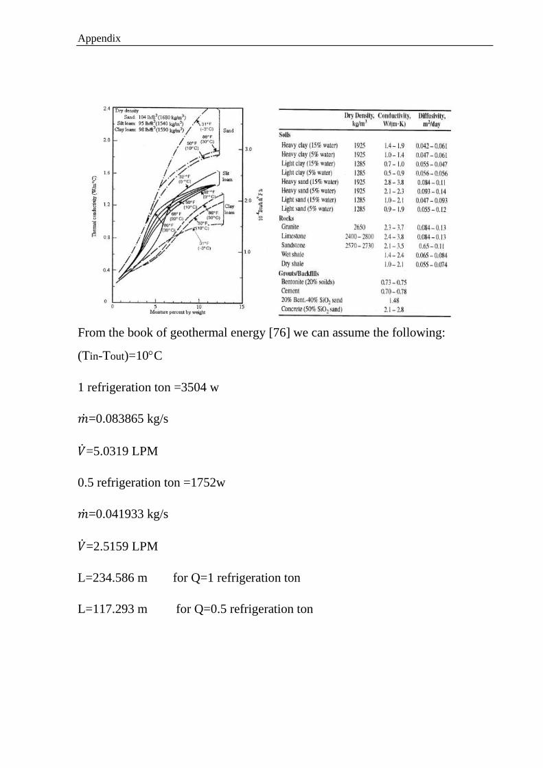
Appendix
From the book of geothermal energy [76] we can assume the following:
(Tin-Tout)=10C
1 refrigeration ton =3504 w
��=0.083865 kg/s
��=5.0319 LPM
0.5 refrigeration ton =1752w
��=0.041933 kg/s
��=2.5159 LPM
L=234.586 m for Q=1 refrigeration ton
L=117.293 m for Q=0.5 refrigeration ton
Appendix
We used 200m length of pipe at two layers each layer have 100 m ,so that's
probably the rate of heat transfer Q become less than 3504w for two layers and
less than 1752 w for one layer.
The estimation of the present research problem, needs to estimate the
properties of the used working fluid. The variation of fluid temperature leads to
variation in its properties such as the density, viscosity, specific heat and the
thermal conductivity [75]. In this study, the mentioned properties are estimated
based on the following empirical formulas:
𝑐𝑝 = −0.00000003136 𝑇𝑏5 + 0.00001113 𝑇𝑏
4 − 0.00149 𝑇𝑏3 + 0.1025 −
3.323 𝑇𝑏 + 4217.8
𝜇 = −0.00000000254 𝑇𝑏3 + 0.00000057 𝑇𝑏
2 − 0.0000465 𝑇𝑏 + 0.001746
𝐾 = −0.000009484 𝑇𝑏2 − 0.002136 𝑇𝑏 + 0.56
𝜌 = −0.000000179 𝑇𝑏4 + 0.0000512 𝑇𝑏
3 − 0.008172𝑇𝑏2 + 0.0659 𝑇𝑏
+999.78
Where:
Tb: fluid bulk temperature (˚C).

Appendix

الخلاصة
جيد نقل على الحصول لغرض سنوات مدى وعلى الحرارة لنقل تقنيات عدة اختبار تم
لنواع الرض تحت الحرارية المبادلات التقنيات هذه ومن , منخفضة تشغيل وتكلفة للحرارة
التربة أعماق إلى لهابداخ السوائل حرارة نقل على تعتمد والتي لاستخدامها مختلفة وأغراض
.صحيح والعكس
لتقليل مغلق كنظام الطبقتين ذو الرض تحت الفقي الحراري المبادل واختبار تصميم تم
لدفن كافية مساحة إلى يحتاج , واحدة بطبقة أفقية حرارية مبادلات تركيب. المطلوبة المساحة
الرض تحت الحرارية لمبادلاتا من النوع لهذا الاقتصادية التكلفة من يزيد مما , المبادل
.(الحيان بعض في كافية مساحة وجود عدم) الفقية الحرارية المبادلات عيوب أحد تعد والتي
المحدد العمق على النسبي ثباتها ولوحظ , العام خلال التربة حرارة درجة انحدار تسجيل تم
ومعرفة التربة نفس من لعينة الحراري التوصيل قياس إلى بالإضافة , م 3.5ى إل م 2 من
مم 16 خارجي بقطر من نوع بولي اثلين متعدد الطبقات وانابيب ماستخدا تم.خصائصها
.طبقة لكل م 100 وبطول مم 2 وبسمك
الشبكتين بيبانا تواجه حيث , متر 100 شبكة كل طول اعوج شكل على شبكتين تصميم تم
على للحصول للأنابيب التلامس مساحة لزيادة (V شكل على) متدرج بترتيب البعض بعضها
وإدخال البعاد ثنائي نظام بافتراض , COMSOL برنامج وباستخدام. برأك حرارة نقل
( 0.5-0.3) لتكون النابيب بين المثلى المسافة اقتراح تم , والتربة للأنابيب التصميم خصائص
GHE .متر لتصميم المبادل الحراري الارضي0.4وتم اختيار البعد ,متر
النظام أنابيب من الثانية والطبقة أمتار 3 عمق ىعل النظام أنابيب من الولى الطبقة دفن تم
ثم حدة على طبقة كل على الاختبارات إجراء وتم , الرض سطح من متر 2.5 عمق على
مئوية درجة 50 و 40 و 30 من الداخل الماء حرارة درجة تغيير طريق عن , معا للطبقتين
الفترة في تحقيقها تم تيوال دقيقة/ لتر 5 و 4 و 3 و 2 من مختلفة تدفق وبمعدلاتقريبا ت
.حرارة المنطقة شهور أشد في التبريد لغرض(. 22/7/2019 - 12/6/2019)
عالية حرارة درجة فرق على الحصول تم , المزدوجة الطبقة وضع في النظام تشغيل عند
متوسطعلى ا يكون , واحدة طبقة بوضع النظام تشغيل وعند ,( مئوية درجة 15.96 المتوسط)

, والثانية الولى الطبقة بالنسبة مئوية درجة( 13.4) و( 15.8) الناتج لحرارةا درجة فرق
مختلفة ظروف ظل في , التوالي على
, قيمة أعلى لتسجيل الطبقتين لكلا النظام اختبار تم ,( COP) الداء معامل تسجيل أجل من
والثانية الولى للطبقتين 5.2 , 5.9 و الطبقات ثنائي التشغيل وضع في 8.59 (COP) وكان
على أنبوب طبقة كل اختبار عند التدفق زيادة بسبب , الظروف نفس في التوالي على الطبقات
.معا المزدوجة الطبقات باختبار مقارنة , حدة

الأرض تحت حراري لمبادل تجريبية دراسة
بطبقتين
رسالة مقدمة الى
في تكنلوجيا الماجستير متطلبات نيل درجة جزء من ك وىقسم هندسة تقنيات ميكانيك الق
الحراريات في هندسة تقنيات ميكانيك القوى
تقدم بها
زهراء صالح عبد زيد بكالوريوس في هندسة تقنيات السيارات
إشرافب
2020 – اغسطس
جمهورية العراق
وزارة التعليم العالي والبحث العلمي
جامعة الفرات الاوسط التقنية
نجف -الكلية التقنية الهندسية
الدكتور المساعد الاستاذ
تحسين علي حسين
الدكتورالمساعد الاستاذ
علي نجاح كاظم