experimental study on machine learning with approximation
TRANSCRIPT

Experimental Study on Machine Learning with Approximation to Data Streams
JIANI JIANG
KTH ROYAL INSTITUTE OF TECHNOLOGY SCHOOL OF ELECTRICAL ENGINEERING AND COMPUTER SCIENCE

www.k th .se

Abstract
Realtime transferring of data streams enables many data analytics and machine learning applications in the areas of e.g. massive IoT and industrial automation. Big data volume of those streams is a significant burden or overhead not only to the transportation network, but also to the corresponding application servers. Therefore, researchers and scientists focus on reducing the amount of data needed to be transferred via data compressions and approximations. Data compression techniques like lossy compression can significantly reduce data volume with the price of data information loss. Meanwhile, how to do data compression is highly dependent on the corresponding applications. However, when apply the decompressed data in some data analysis application like machine learning, the results may be affected due to the information loss. In this paper, the author did a study on the impact of data compression to the machine learning applications. In particular, from the experimental perspective, it shows the tradeoff among the approximation error bound, compression ratio and the prediction accuracy of multiple machine learning methods. The author believes that, with proper choice, data compression can dramatically reduce the amount of data transferred with limited impact on the machine learning applications. Keywords
Data Streaming; Time Series; Data Compression; Machine Learning; Efficient Data Transportation

Abstract
Realtidsöverföring av dataströmmar möjliggör många dataanalyser och maskininlärningsapplikationer inom områdena t.ex. massiv IoT och industriell automatisering. Stor datavolym för dessa strömmar är en betydande börda eller omkostnad inte bara för transportnätet utan också för motsvarande applikationsservrar. Därför fokuserar forskare och forskare om att minska mängden data som behövs för att överföras via datakomprimeringar och approximationer. Datakomprimeringstekniker som förlustkomprimering kan minska datavolymen betydligt med priset för datainformation. Samtidigt är datakomprimering mycket beroende av motsvarande applikationer. Men när du använder dekomprimerade data i en viss dataanalysapplikation som maskininlärning, kan resultaten påverkas på grund av informationsförlusten. I denna artikel gjorde författaren en studie om effekterna av datakomprimering på maskininlärningsapplikationerna. I synnerhet, från det experimentella perspektivet, visar det avvägningen mellan tillnärmningsfelbundet, kompressionsförhållande och förutsägbarhetsnoggrannheten för flera maskininlärningsmetoder. Författaren anser att datakomprimering med rätt val dramatiskt kan minska mängden data som överförs med begränsad inverkan på maskininlärningsapplikationerna. Nyckelord Dataströmning; Tidsföljder; Datakomprimering; Maskininlärning; Effektiv datatranspor

i
Table of Contents
1 Introduction ...................................................................... 1 1.1 Background ........................................................................................................ 1 1.2 Problem statement ......................................................................................... 2 1.3 Purpose .......................................................................................................... 3 1.4 Goal ................................................................................................................ 3
1.4.1 Benefits, Ethics and Sustainability ............................................................ 4 1.5 Methodology .................................................................................................. 4 1.6 Delimitations ................................................................................................. 5 1.7 Reference Work ............................................................................................. 5 1.8 Outline ........................................................................................................... 6
2 Literature Study ................................................................ 7 2.1 Time Series ..................................................................................................... 7 2.2 Data Compression .......................................................................................... 7
2.2.1 Lossless Compression ................................................................................ 7 2.2.2 Lossy Compression ................................................................................... 11
2.3 Machine Learning ........................................................................................ 13 2.3.1 Linear regression ..................................................................................... 13 2.3.2 Logistic regression ................................................................................... 15 2.3.3 Random forest regression ........................................................................ 15 2.3.4 k-Nearest Neighbors regression .............................................................. 16 2.3.5 Recurrent neural network ........................................................................ 17 2.3.6 Long short-term memory ........................................................................ 18
2.4 Summary ...................................................................................................... 19
3 Methodology .................................................................... 20 3.1 Approach ..................................................................................................... 20
3.1.1 Compression algorithm to be used ......................................................... 20 3.1.2 Machine learning algorithms to be used ................................................. 21
3.2 Software ....................................................................................................... 21 3.2.1 Enclosed Environment ............................................................................ 22 3.2.2 Acaconda .................................................................................................. 22 3.2.3 Jupyter Notebook .................................................................................... 22
3.3 Evaluation Outline ....................................................................................... 23 3.3.1 Testbed ..................................................................................................... 23 3.3.2 Test Cases ................................................................................................. 23 3.3.3 Evaluation measurement ......................................................................... 24
3.4 Data Collection ............................................................................................. 26 3.4.1 Temperature-forecasting ......................................................................... 26
4 Implementation .............................................................. 28 4.1.1 System Overview ......................................................................................28 4.1.2 PLA compressor Module ..........................................................................28 4.1.3 PLA Decompressor Module ..................................................................... 33 4.1.4 Machine Learning Module ....................................................................... 35
5 Results ............................................................................. 39 5.1 Experiment result of SC-I ............................................................................ 39 5.2 Experiment result of SC-II ........................................................................... 44

ii
6 Conclusions ..................................................................... 47 6.1 Future work .................................................................................................. 47
7 References ....................................................................... 49

1
List of Abbreviations
AI artificial intelligence
IoT Internet of Things
PLA Piecewise Linear Approximation
PAA Piecewise Aggregate Approximation
DNNs deep neural networks
DFT Discrete Fourier Transform
HC Huffman coding
AC arithmetic coding
SAX Symbolic Aggregate Approximation
k-NN k-Nearest Neighbors
RNN Recurrent neural network
LSTM long short-term memory
TP True Positive TN True Negative FP False Positive FN False Negative MSE Mean Squared Error MAE Mean Absolute Error

2
Acknowledgement
I would like to thank my supervisor at Ericsson, Zhang Fu, for his guidance and help during the period of the thesis. Also, I would like to thank my KTH examiner Jiajia Chen and supervisor Yuxin Cheng for their review and feedback. In addition, I would like to give my appreciations to Ericsson research team and my manager Patrick Sellstedt for their valuable discussions of the thesis. Lastly, I want to thank my parents for continuous support and trust me without a doubt.

1
1 Introduction
Big data is used in many areas, including artificial intelligence (AI), Internet of Things (IoT), or the industrial internet. Transmission, management and analysis of real-world streamed data is a great challenge for people at present, due to countless worldwide sensors like GPS, lasers, or speedometer, etc. Time series data processing and real-time data analysis are essential for real-world applications. Time series is common in the real world, such as weather information, car activity tracking, real-time throughput of the network, etc. It is the data that can been observed at different points in time [1]. Compression techniques could be used to handle big worldwide data by efficiently saving storage space and transmitted bandwidth. Compression methods are basically lossless compression and lossy compression. For time series big data, some loss of less critical information could bring a much smaller size of data, result in a lower transmission and storage cost. Nonetheless, less accurate data might make an impact on further data analysis. For example, it may cause a lower predict precision in an appropriate machine learning model compared to original data. To realize efficient and fast data transmission and analysis, the key is to apply machine learning applications with data compression technologies. The previous researches devoted to the improvement in compression techniques or machine learning algorithms but overlooked their effect might have been each other. This paper concentrates on finding the most significant influence that might have been each other when implementing two techniques for applications.
1.1 Background
High-performance compression techniques are essential to today's scientific research due to the massive volume of data with limited storage space and limited I/O bandwidth energy to access [2]. Mainstream compression modes are basically lossless compression and lossy compression. Lossless compression refers to compression algorithms that apply data coding or encrypting without information loss. By using lossless compression, data can be reconstructed entirely at the receiving end — many previous types of research devoted to it, which leads to more and more unique algorithms. One of the most popular dictionary algorithms is Lempel-Ziv compression with simplicity and efficient compression ratios [3]. Another type of lossless compression is entropy type. Entropy methods like Huffman coding [4], arithmetic coding [5], and Shannon-Fano encoding [6] are beneficial for lossless data compression as well. However, lossless compression cannot guarantee a perfect reducing size due to the compromise of data fidelity, while lossy compression techniques make up the requirement. Lossy compression techniques focus on reducing data volume by ignoring less critical data information. In this case, a compression ratio can be adjusted by the trade-off between information loss and expected data volume. By accepting more information loss, it saves more storage space and transmitted

2
bandwidth, with the price of worse irreversible of data. To possibly reduce data volume and transmission bandwidth, data information is lost to a certain level during the compression and decompression process. For time series data, there are two representations of data compression. One is an adaptive data presentation that converts original data to symbolic strings using a global way of presentation. Piecewise Linear Approximation (PLA) is one of the famous algorithms in symbolic methods. Another is non-data adaptive, which approximate data according to its local features, such as Piecewise Aggregate Approximation (PAA) [7]. Streaming big data could be compressed for smaller storage space and lower transmission bandwidth, with the price of dropping nonessential information. However, less accurate data might be further input to some applications, e.g., machine learning models. Machine learning is also an essential tool for time series data analysis; for example, the rainfall information in a month at some locations, or the daily value of a currency exchange rate [8]. When applying the data in machine learning modes, it’s better to get predictions or decisions with higher precision for applications effetely. It requires the accuracy and integrity of both training and testing datasets, and appropriate algorithms and models. When lossy data is input to one machine learning model as a training set, what butterfly effect will be produced to further predictions of the similar biased testing set? Or, if we use the original data as the training set, how much deviation will it cause when applying the testing set with biased data? In this paper, the answers are found in previous questions. As the author shall demonstrate, error bounds of effective compression techniques could control the compression ratio and degree of information loss, and further control the accuracy of data prediction in machine learning. For time series data, the error bound of the compression could be adjusted in real time by the tradeoff between compression ratio and prediction accuracy. This kind of framework is more adaptive to real-world applications.
1.2 Problem statement
Time series big data could be compressed for smaller storage space and lower transmission bandwidth, with the price of dropping nonessential information. In a data pipeline, the less accurate data might be further input to a machine learning model. Here I design two related scenarios:
• A machine learning model is well-trained for a specific big time series data application using accurate historical data. It needs to be further tested and applied with real-time time series data. In order to save transmission and storage costs, a lossy compression method is applied to later collected time series data. In this first scenario, the machine learning model is trained by an accurate training dataset and tested by the lossy testing dataset.
• One machine learning model is required for a specific big time series data application. To save transmission and storage costs as much as

3
possible, a lossy compression method is applied to data processing. In this second scenario, machine learning models are trained and tested by both lossy datasets.
Based on the two scenarios, lossy data is applied to well-trained or untrained machine learning models. This leads to questions about prediction results:
• When using original data as a training set while input the decompressed lossy data as a testing set, what’s the impact on prediction error of test results?
• What's the influence on prediction error when applying lossy data as the training dataset and testing dataset to machine learning models?
To the knowledge of the author, there is no existing solution for an experimental study on prediction errors of machine learning with compression to time series streams. The impact of data compressions on prediction errors of machine learning models is the key point to this paper.
1.3 Purpose
The purpose of the degree project is to analyze the influence of data compression on machine learning models. This, in turn, leads to evaluating and implementing an appropriate compression method for time series streams. In order to compress time series streams, new ideas are injected into existing compression methods. In addition, to analyze as many machine learning algorithms as possible, the author chose the most widely used machine learning algorithms. Different contrast tests are designed to evaluate the real impact of data compression on machine learning.
1.4 Goal
The goals of the degree project are listed as follows:
• Research various data compression methods and techniques that can achieve time series streams compression with a high compression ratio. Investigate the requirement of compressing time series streams and choose a proper compression method for this experiment study.
• Study different machine learning models that used for time series data predictions. Choose the most widely used models with different prediction principles.
• Design and implement compression and decompression modules. Build a data transmission channel between two modules.

4
• Build machine learning models that used for time series prediction and forecasting.
• Design two testing scenarios. Evaluate the framework by measuring the compression ratio of data compression and prediction errors of machine learning.
1.4.1 Benefits, Ethics and Sustainability
Study the experiments of applying data compression techniques to machine learning models has several benefits on energy and research fields. The benefits are:
• This thesis points a new idea of combining data compression and machine learning on time series streams. It is a new angle research of academic horizon.
• This thesis corporate data compression with machine learning, which is good for big data analysis. It can largely save the transmission energy and storage costs.
• It provides a reference for researches and engineers who would like to study or apply machine learning models with compression to time series streams. The evaluation results can also be a guideline as stability estimation to popular machine learning algorithms.
The ethical aspect of the thesis is that this solution doesn’t waste the energy that is used within transmission and storage. However, it may cause information loss on time series streams and leads to further impact on machine learning models. In order to reduce the influence, the author gives experiments and tries to provide a recommendation on data compression and machine learning choices. For sustainability, the economic aspect is that this study can help with energy-saving, which is conducive to sustainable development. To be more specific, it can reduce the costs of data transmission and storage. The reconstructed data can still be useful in data analysis. This is also essential to future significant data development.
1.5 Methodology
The work is based on three phases of literature study, implementation and evaluation. In order to achieve the goals of this thesis, both quantative and qualitative researches are used to evaluate the results. To address the development process of each phase:
• Literature study: This is the first phase of this study. Related work and background materials are studied. First, a study on different data compression for time series streams is done in order to choose an appropriate compression method. Then, materials and tutorials of

5
machine learning algorithms for time series predictions are studied. These steps provide the essential background knowledge that is necessary to design the compression models and build machine learning models. Based on the background, the design of the entire framework is drawing. This consists of 3 models:
o Compression module: Compression module is responsible
for collecting or reading data from local files. The streaming data is immediately input to compression part and the model needs to achieve real time compression and transmission.
o Decompression module: Decompression module acts as the receiver. A socket is built for compression and decompression models for data transmission. Once decompression model receives the streaming data, it needs to decompress it as soon as possible and output it to local files in real time.
o Machine learning module: In the machine learning module, researchers can invoke local files in the decompression module side as the input datasets. Two scenarios are designed in machine learning module to achieve contrast experiments.
• Implementation: In this phase, the aforementioned modules are implemented in distribution. The aim of this phase is to build the designed framework and make it achieves the requirements. The compression method and machine learning algorithms should both be adjusted for time series streaming data.
• Evaluation: This phase evaluates performances of data compression and machine learning using the pre-determined key performance indicators. The evaluation is measured in two testing scenarios as aforementioned design.
1.6 Delimitations
In this thesis, the author only focuses on time series streams compression and analysis. In this case, only one typical time series data is tested in this experiment. Therefore, the results can only be applied to time series data with a similar trend and distribution. According to the features of data, compression ratio and prediction results can be disparate, even using the same framework. In addition, the prediction results can be diverse due to different parameter adjustments. In this thesis, the author adjusted most parameters to obtain a good prediction result. A detailed description of models and related parameters will be provided in bellowing chapter 4 as a reference.
1.7 Reference Work
Authors in [9] present an compression method that produces the optimal PLA in terms of representation size while satisfying the pre-determined max-error

6
bound. In this paper, it basically follows the proposed algorithm to do the PLA processing on our dataset. S. Teerapittayanon et al. [10] propose to distribute deep neural networks (DNNs) over distributed computing hierarchies. The purpose is to reduce communication cost compared with the traditional method of offloading raw sensor data to be processed in the cloud. However, the data transferred between consecutive layers in DNN can only be used by DNN; it can hardly be used by other machine learning methods. Whereas data approximation, such as PLA, is independent of machine learning algorithms. B. Havers et al. [11] propose to use PLA in compressing the data transferred in the vehicular network. They find similar results as in this paper that the compression method can reduce the data size dramatically, and the corresponding data analysis application can still achieve excellent performance. However, their study only focuses on the impact of distance-based clustering, e.g., single-linkage clustering, whereas in this paper, the author studies the impact of data compression on multiple machine learning methods.
1.8 Outline
The structure of this paper is outlined as follows:
• Chapter 2 presents the research and literature of compression methods to time series streams, including the study on lossless and lossy compression methods. The backgrounds of time series and machine learning are also introduced in Chapter 2.
• Chapter 3 describes the methodologies of development and evaluation. It also introduces the dataset, compression method and machine learning algorithms that used in this thesis.
• Chapter 4 gives the detailed implementation of data compression and decompression modules. Also, the build of machine learning models and parameter choice will be presented in this chapter.
• Chapter 5 shows the evaluation and analysis of two testing scenarios. The compression ratio and prediction errors are the key evaluation indexes for data compression and machine learning.
• Chapter 6 concludes the work according to the aforementioned goals. It also gives limitations and suggestions to future work.

7
2 Literature Study
In this chapter, a detailed knowledge for readers to understand time series data, data compression, and machine learning is presented together with related work. In addition, the merits and demerits of each technique are listed for comparison. The author gives a clear indication of techniques that are adopted in this thesis based on its pros and cons.
2.1 Time Series
The observation of data at distinct time points, including the continuous and discrete forms, is called time series data. For example, the audio waveform of a piece of music can be observed as a continuous time series data. Analysis of time series on scientific applications is essential to deal with real problems and improve the quality of application services. While time series data have a natural ordering related to observations, it can also be viewed as streaming data. For continuous time series data, a proper choice of data representation is essential. There is a lot of previous work related to data mining and time series representation, for example, the Discrete Fourier Transform (DFT) [12], Piecewise Linear Approximation (PLA) [9], Piecewise Aggregate Approximation (PAA) [13], etc. For discrete time series, although the majority work on streaming data tacitly approve that the data is discrete, the real-valued data still can be represented by the mentioned algorithms for the purpose of compression. In this paper, discrete time series data is applied for mainly research, while continuous data processing is left for further work.
2.2 Data Compression
By encoding data, data compression can represent the original data with fewer bits or values. Effective compression techniques are essential for big data storage and transmission. So far, it is commonly used for music compression (MP3 [14], WMA [15]), images compression (JPEG [16], PNG [17]), video compression (MPEG-4 [15]), etc. Lossless compression and lossy compression are two types of data compression. Lossless compression encodes data by reducing data redundancy without any information loss, while lossy compression approximates data by dropping less important information.
2.2.1 Lossless Compression
Lossless compression can reduce the data volume without any information loss, which means that the original data and decompressed data is the same. Usually, a lossless compression model will first monitor the statistical property (e.g., frequency of occurrence) of input data, then build up a mapping tree or model to encode input data. The modern lossless compression is mainly based on two approaches to entropy coding: Huffman coding (HC) and arithmetic coding (AC) [18]. Later, the Asymmetric numeral systems approach was introduced with a high performance of combining the

8
fast speed of Huffman with the high compression rate of arithmetic coding [19].
2.2.1.1 Huffman Coding
Huffman coding is a method to reduce information redundancy to realize lossless compression. In this way, a symbol or a sequence of symbols related to input data is used as the representation. It was introduced by David A. Huffman when he was a student at MIT and published his paper in 1952 [20]. So far, many versions of Huffman coding were promoted, including adaptive Huffman coding [21], Length-limited Huffman coding [22], etc. In the coding process, it is vital to avoid the situation that two input messages are coded in a way that one code digits as the first part of the other code digits. For example, if the ensemble code of an information source is 01, 11, 101, 111, 102. When a sequence of messages comes as 111101102, it can be explained as 11-11-01-102 or 111-101-102. In this case, it is not sure that whether the message 11 has been received or it is only the first two digits of 111. Therefore, two restrictions are vital for Huffman coding [20]:
1. No two messages consist of identical arrangements of coding digits;
2. In the construction process, no additional indication is necessary to specify the begins and ends of a message code once the starting point is known.
Thus, Huffman coding always finds a prefix-free binary code to reduce message redundancy. A Huffman tree is constructed before encoding, and each message could be encoded by a minimum expected codeword based on the tree, as shown in Figure 2.1.
Figure 2.1: Example for Huffman Tree Construction

9
When a source of information is monitored for a period, the frequency of different messages can be detected (e.g. {y: 0.025, r: 0.025, f: 0.05, q: 0.1, n: 0.1, u: 0.2, c: 0.2, e: 0.3} as shown in Figure 2.1). The two minimum frequency nodes are extracted to be a new internal node with the frequency equals to the sum of the chosen two minimum frequency. Then, extract another two minimum frequency nodes again and repeat the last step until there is only one node. The tree can be traced back and assigned different bits to branches. The final Huffman code of this example is shown in Table 2.1. For instance, when a message comes as “frequency”, the final transmitted codeword will be 111110 1111110 0 11110 110 0 1110 10 1111111.
Table 2.1: Example for Huffman Codeword Message Code y 1111111 r 1111110 f 111110 q 11110 n 1110 u 110 c 10 e 0
For decompression, information is needed to reconstruct the Huffman tree. For instance, the frequency of every message could be prepended to the compression stream for the Huffman tree reconstruction. Once the tree is ready, the codeword can be translated by traversing the tree. In this example, 0 can be observed as the terminator; the next bit followed with 0 is the start for the next symbol. So, by the reconstructed tree, the input bits can be translated to the original message "frequency". Huffman coding is one of the simplest algorithms for data compression to understand and implement. It has a fast speed but approximates probabilities with powers of 2, and this leads to relatively low compression rates [18]. Additionally, when the ensemble frequencies change with time, or we can't know frequencies a priori, Huffman coding is not the right choice.
2.2.1.2 Arithmetic Coding
Arithmetic coding is another simplified approach for lossless data compression. Similar to Huffman coding, arithmetic coding translates symbols with high frequency fewer bits, while not-so-frequently symbols are represented by more bits. The difference is that arithmetic coding uses only one number to represent an entire message. The more not-so-frequency symbols a message contains, the longer the represented number will be. Compare to traditional coding like Huffman, arithmetic coding breaks the convention that each symbol needs to be translated to bits, so that coding more efficiently [23]. Therefore, arithmetic coding can quickly achieve the theoretical compression rate limit, which is also called Shannon entropy [18].

10
In arithmetic coding, a message is usually encoded to a number in the interval between 0 and 1. As each symbol is processed, the represented interval is narrower [23]. For example, there is an information source that generates messages contain symbols {c, e, n, u, q, f, r, y}; the frequency of each symbol is monitored in advance, as shown in Table 2.2.
Table 2.2: Example for Symbol Frequencies Symbol Frequency Range e 0.3 [0, 0.3)
c 0.2 [0.3, 0.5) u 0.2 [0.5, 0.7) n 0.1 [0.7, 0.8)
q 0.1 [0.8, 0.9) f 0.05 [0.9, 0.95) r 0.025 [0.95, 0.975)
y 0.025 [0.975, 1) The frequency of each symbol decided the subrange on behalf of this symbol. Both encoder and decoder have the same partition related to symbol frequencies. Again, when a message comes as “frequency”, in Huffman coding, each symbol needs an individual translation. However, in arithmetic coding, one final number will be chosen to represent the entire message, as shown in Figure 2.2.

11
Figure 2.2: Example of Arithmetic Coding
Initially, the interval is [0, 1) and divided to multiple subintervals according to the frequencies of symbols. After seeing symbol f, f is observed inside the interval [0.9, 0.95) and the model is scaled into this range. Then, when the next symbol r comes, it is observed in the new range [0.9, 0.95) with the same ratio. Again, symbol r is in the range of [0.94875, 0.9475), and the model is scaled in the new range. This step is repeated until the last one is converted. When the last symbol y comes, it is observed in the range of [0.94782044, 0.94782043875). Finally, a random number in this range will be chosen to send. Proceeding like this, the decoder can identify the whole message [23]. For decoding process, the decoder needs to know when to stop decoding. Because the message could be decoded like “frequencyyyyyy…” without an end mark. Therefore, it need a special EOF symbol known to both encoder and decoder to end the processes. Normally, dot marks like a period or exclamation mark, are adopted to indicate the end of a message. When decoders see this EOF symbol, it stops decoding right away. Arithmetic coding has a relatively high compression ratio but limited with its complexity and computing time. Also, the precision of codeword should be guaranteed to correctly decoding, thus limiting the number of symbols in a message.
2.2.2 Lossy Compression
Lossy compression is another data encoding technique where the data is approximated or discarded to reduce the data volume. Compared to lossless compression, lossy compression is superior to compress data to a tiny size by dropping some less critical information. Therefore, lossy compression is always irreversible. Due to high requirements of compression in media files, lossy compression is always applied to audio compression, video compression, and image compression. However, lossy compression is less suitable for text and natural language because of its irreversible characteristics. For time series data collected from detecting devices like sensors, small information loss is acceptable. For example, for temperature data that detected from sensors, a little bit shift of values (The detected temperature value is 10 degree centigrade, while the received value is 11 degree centigrade.) is innocuous.
2.2.2.1 Symbolic Aggregate Approximation
Symbolic Aggregate Approximation (SAX) is an advanced usage of the Piecewise Aggregate Approximation (PAA) algorithm. SAX can approximate a series of time series data into a segment of symbols to reduce data sizes significantly. The algorithm has two steps: first transforms the data to PAA representations, and then symbolic the PAA representation into a discrete string [7].

12
Figure 2.3: Example of Piecewise Aggregate Approximation
PAA can represent a time series data into a n-dimensional space by n vectors, as shown in Figure 2.3. It is also a method to dimension reduction. By PAA representations, a time series data of w dimensions can be decreased to n dimensions where n is far less than w. To be specific, a time series data is divided to n equal sized frames, and the mean value of the data that within the frame is used to represent this frame. Then a vector of the mean value can be obtained to represent this frame as a dimensional reduced representation [7].
Figure 2.4: Discretization of PAA representations
While transforming time series data into a PAA representation, vectors can be discretized to a further symbolic form. It can be proved that the normalized time series meet a Gaussian distribution [24]. So the breakpoints which make equal-sized areas under the Gaussian curve can be found and PAA representations can be discretized in the following way: The PAA coefficients located under the smaller breakpoint are mapped to symbol "B". Similarly, the
13
PAA coefficients within the range between the smaller and the larger breakpoints are mapped to symbol "A". And the PAA coefficients above the more significant breakpoint are mapped to symbol "C". To the example shown in Figure 2.4, the time series data is finally mapped to a segment of symbols “AABACC”.
2.2.2.2 Piecewise Linear Approximation
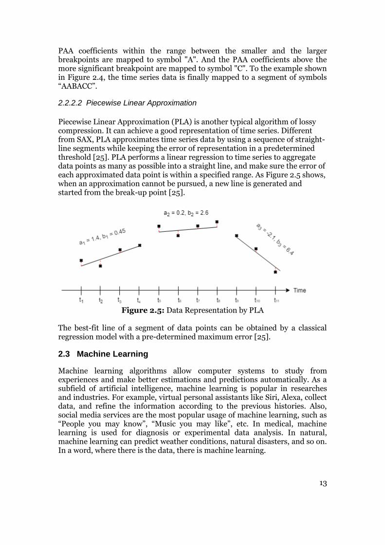
Piecewise Linear Approximation (PLA) is another typical algorithm of lossy compression. It can achieve a good representation of time series. Different from SAX, PLA approximates time series data by using a sequence of straight-line segments while keeping the error of representation in a predetermined threshold [25]. PLA performs a linear regression to time series to aggregate data points as many as possible into a straight line, and make sure the error of each approximated data point is within a specified range. As Figure 2.5 shows, when an approximation cannot be pursued, a new line is generated and started from the break-up point [25].
Figure 2.5: Data Representation by PLA
The best-fit line of a segment of data points can be obtained by a classical regression model with a pre-determined maximum error [25].
2.3 Machine Learning
Machine learning algorithms allow computer systems to study from experiences and make better estimations and predictions automatically. As a subfield of artificial intelligence, machine learning is popular in researches and industries. For example, virtual personal assistants like Siri, Alexa, collect data, and refine the information according to the previous histories. Also, social media services are the most popular usage of machine learning, such as “People you may know”, “Music you may like”, etc. In medical, machine learning is used for diagnosis or experimental data analysis. In natural, machine learning can predict weather conditions, natural disasters, and so on. In a word, where there is the data, there is machine learning.
14
Machine learning algorithms are mainly categorized as unsupervised learning, supervised learning, and deep learning. When information is neither classified nor labeled, unsupervised learning usually find the inner structure of unlabeled data. Typical methods are like hierarchical clustering [26], k-means [27], etc. While supervised learning can learn from the past and apply to new data by using labeled information. Popular algorithms for supervised learning are linear regression [28], logistic regression [29], naïve Bayes [30], decision trees [31], k-nearest neighbor algorithm [32], etc. With the analysis of the training dataset, supervised learning algorithms learn and improve functions to estimate output values. Trained models are further tuned by validation datasets, and model performances are tested by test datasets. Time series analysis is to find meaningful statistics from data, and time series forecasting is to predict future values according to historical data. Therefore, time series data can be applied to the following supervised learning algorithms.
2.3.1 Linear regression
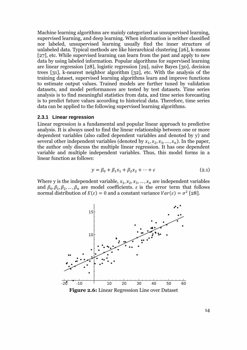
Linear regression is a fundamental and popular linear approach to predictive analysis. It is always used to find the linear relationship between one or more dependent variables (also called dependent variables and denoted by y) and several other independent variables (denoted by 𝑥1, 𝑥2, 𝑥3, … , 𝑥𝑛). In the paper, the author only discuss the multiple linear regression. It has one dependent variable and multiple independent variables. Thus, this model forms in a linear function as follows: 𝑦 = 𝛽0 + 𝛽1𝑥1 + 𝛽2𝑥2 + ⋯+ 𝜀 (2.1) Where y is the independent variable, 𝑥1, 𝑥2, 𝑥3, … , 𝑥𝑛 are independent variables and 𝛽0, 𝛽1, 𝛽2, … , 𝛽𝑛 are model coefficients. 𝜀 is the error term that follows normal distribution of 𝐸(𝜀) = 0 and a constant variance 𝑉𝑎𝑟(𝜀) = 𝜎2 [28].
Figure 2.6: Linear Regression Line over Dataset

15
Once the relationship between dependent y and independent 𝑥𝑖 is found, as Figure 2.6 shows, we can easily predict y values based on a set of values of 𝑥𝑖. For example, in one of the experiments in this thesis, the author uses many independent variables, including atmospheric pressure, relative humidity, water vapor pressure, and so on, to try to find a causal relationship with a dependent variable temperature and predict temperature values according to the independent features.
2.3.2 Logistic regression
Logistic regression is most associated with a logistic or binary function. It usually categorizes results into two classes like true/false, positive/negative, win/lose, etc. by estimating probabilities of inputs. For example, if the estimated probability of input is higher than 0.5, the result would be positive, and vice versa. In addition, the logistic model can be extended to modeling multiple classes prediction, such as predicting whether the next day is a sunny day, rainy day, cloudy day, snowy day, etc. by assigning distinct probabilities to every class. Similar to linear regression, logistic regression also finds the relationship between one or more dependent variables and several other independent variables as Formula 3.1 shows. Then take the output y as an input to the standard logistic function - sigmoid function [33]:
𝑃(𝑦) =𝑒𝑦
𝑒𝑦 + 1=
1
1 + 𝑒−𝑦 (2.2)
Where y is the output of the linear function, but the input of a sigmoid function, P(y) is the output probability. Figure 2.7 shows the standard sigmoid function. It takes any real input and outputs values between 0 and 1. In the logistic model, it takes outputs as probabilities and matching to 0 or 1. For example, when 𝑃(𝑦𝑖) = 0.3 and it is less than 0.5, the prediction is matched to 0.
Figure 2.7: Standard Sigmoid Function
2.3.3 Random forest regression

16
The key to the random forest is to create a forest randomly, where an ensemble of decision trees host. The algorithm uses the bagging [34] resampling technique to randomly choose data from the same original training set to generate a new training subset. In this way, it can generate multiple subsets from the original training set randomly and with replacement. Using bagging to generate subsets can also avoiding the high variance problem of a single decision tree. With high variance, a model can be easily affected even with only small changes in the training dataset.
Figure 2.8: Structure of Random Forest Model
Then each of the training subsets can be used to generate a decision tree and constitute a random forest finally. As Figure 2.8 shows, the k decision trees make up a random forest, and the prediction result of testing data is determined by voting or mean value. By merging many decision trees together, it can always get a more accurate and stable result comparing to a single decision tree.
2.3.4 k-Nearest Neighbors regression
The k-Nearest Neighbors (k-NN) regression assumes that similar things should be close to each other, which is called “feature similarity”. Different from linear regression and logistic regression, it is a non-parameter method. Instead of probability estimation, it uses feature space, which is also called vector space in linear algebra.
17
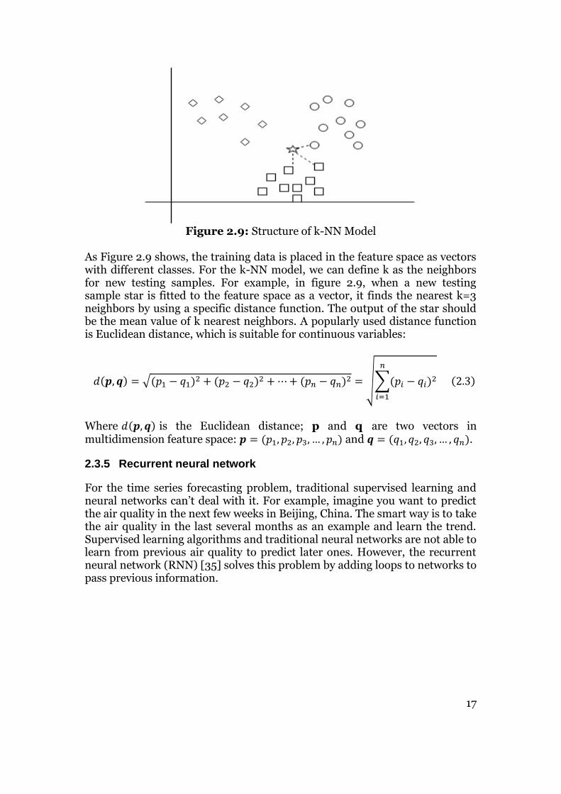
Figure 2.9: Structure of k-NN Model
As Figure 2.9 shows, the training data is placed in the feature space as vectors with different classes. For the k-NN model, we can define k as the neighbors for new testing samples. For example, in figure 2.9, when a new testing sample star is fitted to the feature space as a vector, it finds the nearest k=3 neighbors by using a specific distance function. The output of the star should be the mean value of k nearest neighbors. A popularly used distance function is Euclidean distance, which is suitable for continuous variables:
𝑑(𝒑, 𝒒) = √(𝑝1 − 𝑞1)2 + (𝑝2 − 𝑞2)2 + ⋯+ (𝑝𝑛 − 𝑞𝑛)2 = √∑(𝑝𝑖 − 𝑞𝑖)2
𝑛
𝑖=1
(2.3)
Where 𝑑(𝒑, 𝒒) is the Euclidean distance; p and q are two vectors in multidimension feature space: 𝒑 = (𝑝1, 𝑝2, 𝑝3, … , 𝑝𝑛) and 𝒒 = (𝑞1, 𝑞2, 𝑞3, … , 𝑞𝑛).
2.3.5 Recurrent neural network
For the time series forecasting problem, traditional supervised learning and neural networks can’t deal with it. For example, imagine you want to predict the air quality in the next few weeks in Beijing, China. The smart way is to take the air quality in the last several months as an example and learn the trend. Supervised learning algorithms and traditional neural networks are not able to learn from previous air quality to predict later ones. However, the recurrent neural network (RNN) [35] solves this problem by adding loops to networks to pass previous information.

18
Figure 2.10: Structure of RNN Model
As Figure 2.10 shows, in the RNN model, neuron-like nodes are connected into a successive RNN layer. Each neuron accepts a time-ordered input and the last state, then output the result in real-time and pass the updated state to the next neuron. The result is generated by activation function with taking both the weighted input and last state as inputs. Also, the state will be updated based on the current input and processed to the next neuron. In this way, the memory can pass through all the way to the end of the neuron. Due to its memory dependent feature, RNN is very successive in natural language processing and time series forecasting.
2.3.6 Long short-term memory
Long short-term memory (LSTM) [36]is an improvement of the RNN algorithm. Because in the computations of parameter optimization, it uses finite-precision numbers. This can cause the gradients to be extremely small or large. LSTM model solves the vanishing gradient problem by introducing three different gates, but it still has an exploding gradient problem.
Figure 2.11: Structure of LSTM Model

19
In a prediction application, sometimes it only needs recent memories to estimate the next event, sometimes long memories are required. LSTM can realize the control function by adding an input gate, output gate, and forget gate. As Figure 2.11 shows, a neuron includes a cell 𝑐𝑡, input gate 𝑖𝑡, output gate 𝑜𝑡 , and forget gate 𝑓𝑡 . Therefore, the cell state can be updated by removing or adding information that decided in the previous two steps. Finally, the output gate will output the cell state with a filter and only output the part that is required. Comparing to RNN, LSTM has a more complex structure but a better performance. It is well-suited on time series data processing and prediction applications because the uncertain duration between some important time events commonly exists in time series.
2.4 Summary
In this chapter, the author first introduced the basic concepts of time series data and how it should be compressed. Secondly, the author explained several classic lossless and lossy compression methods and analyzed them to find a suitable compression algorithm for time series. Finally, the critical idea of machine learning was mentioned, and some proper machine learning algorithms for time series data were listed.
20
3 Methodology
Chapter 3 describes the research methodologies that are used in the degree project. Methods used in software developing, reliability evaluating, and data analyzing are explained. In section 3.1, the author shows the choice of compression methods and machine learning algorithms based on problem formulations. In section 3.2, the software used in this thesis is presented. Section 3.3 gives a detail description of testing scenario design, and section 3.4 shows the dataset that is applied in the experiments.
3.1 Approach
This Section introduces the chosen compression method and reasons. Meanwhile, a brief explanation of the machine learning algorithms implemented in this project is given in Section 3.1.2.
3.1.1 Compression algorithm to be used
The chosen compression algorithm is PLA. Many time series applications, like temperature forecasting, location detection, and network traffic monitoring, can tolerant some information loss to achieve high compression ratios. Also, time series have excellent value continuity. Therefore, it's suitable to apply with a lossy compression method. Comparing PAA, SAX, and PLA, the author, chose PLA as the compression method in this thesis. The reasons are given as follows:
• Compare to PAA and SAX, PLA has an adaptive ability to compress data in a flexible version. If there is a vast difference between data values, PLA fits them with shorter but more lines, while PAA and SAX ignore data trends and rigidly calculates a mean value for each divided frame.
• Values of time series usually have a good continuity, for example, location detection of object movements, daily temperature monitoring, etc. The collected data is discrete but changes continuously. PLA uses the ‘best fit line’ to get as near to data points as possible. In this case, PLA can better make use of value tendencies of time series and achieve a higher compression ratio.
• Another reason for choosing PLA is due to its excellent error-controlled function. SAX can reach different compression ratios by adjusting the size of each frame, but it can't guarantee the deviation of every single point is within a threshold. When PLA generates a line to approximate data points, it dynamically adjusts the line after a new point comes in. It makes sure that this line is the best-fit line for compressed points, and the error of every point is smaller than a specific error bound. If a new point is far away from the existing line, or it changes the line without satisfying previous points, this point will be a break-up point.

21
It won't join the existing line anymore. Instead, approximation restarts from the break-up points. In this way, PLA ensures the deviation of every point is under a specified error bound.
3.1.2 Machine learning algorithms to be used
Time series can be applied in both supervised learning and deep learning models to achieve both analysis and forecasting applications. In this paper, I used the most popular supervised learning algorithms and neural network models that can be used for time series streaming data:
• Linear regression is the most typical and simple algorithm that used as a linear approximation for prediction. It tries to get the best linear relationship between the predicted object and other variables (which are the input variables) in the feature space. When the values of input variables are determined, the output of the predicted object is determined by the corresponding linear combination of the input variables.
• Logistic regression is a typical method to classify data using different labels. The main idea of this approach is to model the log-likelihood of the classification outputs as linear functions of the inputs. The model coefficients are estimated by maximizing the log-likelihood of the observed outputs in the training data. This method has an advantage of robustness, although its accuracy might not be as high as other approaches, such as a neural network.
• K-nearest neighbor (k-NN) is trendy in the clustering field. It can be used for both classification and regression, and the prediction outcome is determined by the k nearest neighbors of the predicted object in the feature space. For the case of classification, all k nearest neighbors will vote the object to their own class, and the object will finally be classified into the most voted class. For the case of regression, the regressed value of the predicted object can be calculated by taking the average value of the k nearest neighbors.
• Random forest is an ideal solution for solving classification and regression problems by using a tree-based model. It is an ensemble approach, which could be applied to both classification and regression problems. It is based on averaging the result of an ensemble of decision trees and trained on a different part of training dataset to reduce the variance.
• RNN uses a neural network method for time series forecasting. It takes both the output from previous time steps and input of the current time step. It is used to capture the relation in a time series over time steps. The output of the following time steps will refer to the knowledge from the previous time step and the input of its current time step. More

22
techniques like Long-Short-Term Memory (LSTM) can be applied for tuning the length of previous time steps referred to in prediction results.
• Long short-term memory (LSTM) models for time series forecasting. It is an improvement from RNN by adding more gates to control information that is passed through RNN units. Basically, it adds three gates: input gate, output gate, and forget gate. The input gate controls what new information will be encoded into the cell state. The output gate concerns what information is transferred as input in the following time step. The forget gate considers what information in the cell state to drop out. These three gates work together to keep important information and forget less-essential information. Therefore, LSTM is also an advantage for learning long sequences with long time lags.
3.2 Software
This Section introduces the mainly software that used in this degree project. This includes the experimental environment to deploy the project in and the virtualization tools.
3.2.1 Enclosed Environment
This project is implemented and evaluated in an enclosed virtual environment. In this enclosed environment, the author built a feeder which read information from local files line by line. This can be simulated as a sensor detecting a piece of events. This feeder reads information every 1 second and input data to a light compressor function directly. Also, the input string bytes and output string bytes of light compressor could be monitored to calculate the compression ratios. In this case, the compression ratio of data can be traced. On the receiver side, it takes streaming data as inputs to the decompressor module. The reconstructed data is output and stored in real time under the synchronization mode. The compression and decompression modules are developed in IntelliJ as two independent modules using Java language. For machine learning module, all the machine learning models are built in Jupyter Notebook [37] using Python language. In this module, the author needs to import the local files stored by the decompression module manually. Two testing scenarios are designed in this module for evaluation. For each scenario, independent machine learning models are implemented in different code files. The evaluation of each machine learning model within different scenarios is also built within python files in Jupyter notebook.
3.2.2 Anaconda
Machine learning algorithms are implemented and evaluated in Jupyter Notebook application in Anaconda [38]. Anaconda is an open-source computer software that contributes to Python and R programming languages for data analysis applications like machine learning, data processing, and
23
mining, etc. It has a GUI, Anaconda Navigator, that can allow users to run applications, including JupyterLab [39], Jupyter Notebook, QtConsole [40], and some other applications. In this thesis, the author launched Jupyter Notebook mainly through the Anaconda software.
3.2.3 Jupyter Notebook
Jupyter Notebook is an application that allows users to create, edit, and run code through a web browser. It can be executed both in the local environment without internet access or on a remote server. To using Jupyter Notebook in Anaconda, this application can be opened on the project home page; then, this will trigger a new browser window where Jupyter Notebook files will be listed in its control panel. All the local files can be opened or shut-down by its kernel in the panel. The kernel in Jupyter Notebook is like the engine for a car. The code in the control panel is executed by the kernel. When a code file is opened, the associated kernel will be automatically launched [41]. Lastly, to manage all related files (also called "notebooks", which are computer code and abundant text elements that produced by Jupyter Notebook), the file manager can also be found in the Terminal, Workbench, and Viewer applications.
3.3 Evaluation Outline
This subsection states the evaluations of data compression and machine learning testing, and the way to find the tradeoff between the error bound of compression and the prediction error of machine learning.
3.3.1 Testbed
As mentioned in Section 3.2.2 and 3.2.3, the compression performance is implemented and tested in IntelliJ IDE, and machine learning algorithms run in Jupyter Notebook. The prediction evaluations and virtualizations are also performed in Jupyter Notebook. For the virtual machine where IntelliJ IDE and Jupyter Notebook is running on, it has the following features:
• Operating System: Ubuntu 18.04.1 LTS.
• Kernel: Linux Kernel 4.15.0-46-generic.
• Memory: 18G.
• CPU: 4 Intel Core i7-8650U, 1.9 GHz.
3.3.2 Test Cases
In this thesis, the author designed two testing scenarios for different application requirements. The detailed information of them are described as follows:
3.3.2.1 First testing scenario
The first scenario was designed for the condition of adding a data compression module to a trained machine learning module. In this case, parameters for the model are trained by original data, and the further lossy data should be predicted by using the parameters directly. To simulate this situation, the author designs the first scenario, which is called SC-I.
24
In SC-I, machine learning models are trained by original accurate training dataset. In this step, the original machine learning model can be trained. Then, it is tested by the lossy testing dataset that is compressed with different degrees of error bounds. The error bound is set to 0.5%, 1%, 3%, 5%, 10%, 15% and 20%.
3.3.2.2 Second testing scenario
The second scenario is designed for building a new project that contains the data compression module and machine learning module. In this situation, both training data and testing data are compressed first to reduce data volume. Then the lossy training data is used to train a machine learning model and leave the parameter for lossy testing data. To realize this case, the author designs the second scenario, which is also called SC-II. In SC-II, machine learning models are trained and tested by both lossy data that is compressed in every error bound. The error bound is set to 0.5%, 1%, 3%, 5%, 10%, 15% and 20%.
3.3.3 Evaluation measurement
In the machine learning module, all the data values used in the experiment are first normalized in order to make features of different scales on the same scale. For example, we usually calculate the Euclidean distances among points in k-NN to find the nearest neighbors to do the majority vote. Features with large ranges will take a heavyweight in the calculation led to poor performance. Also, normalized datasets are helpful with speed up the gradient descent converges in neural network models [42]. Thus, the author carried out Z-score Normalization to both training and test datasets. So, the unstructured data can be normalized using the z-score parameter as follows [43]:
𝑦𝑡𝑟𝑎𝑖𝑛′ =
𝑦𝑡𝑟𝑎𝑖𝑛 − ��
𝑠𝑡𝑑 (3.1)
ytest
′
=ytest − E
std (3.2)
Where 𝑦𝑡𝑟𝑎𝑖𝑛 and 𝑦𝑡𝑒𝑠𝑡 are original training and testing data values; 𝑦𝑡𝑟𝑎𝑖𝑛
′ and 𝑦𝑡𝑒𝑠𝑡
′ are Z-score normalized training and testing values; �� stands for the mean value of the training dataset and Std is the standard deviation of the training dataset:
�� =1
𝑁∑𝑦𝑖
𝑁
𝑖=1
(3.3)

25
𝑆𝑡𝑑 = √1
𝑁 − 1∑(𝑦𝑖 − ��)2
𝑁
𝑖=1
(3.4)
After machine learning models are trained by training datasets, expect logistic models, the author evaluates performances of models using testing datasets and calculate errors as follows:
𝑁𝑜𝑟𝑚𝑎𝑙𝑖𝑧𝑒𝑑 𝑀𝐴𝐸 =∑ |��𝑖
′ − 𝑦𝑖′|𝑁
𝑖=1
𝑁
=∑ |
��𝑖 − ��𝑠𝑡𝑑
−𝑦𝑖 − ��𝑠𝑡𝑑
|𝑁𝑖=1
𝑁
= ∑ |��𝑖 − 𝑦𝑖|
𝑁𝑖=1
𝑁 ∗ 𝑠𝑡𝑑 (3.5)
Where ��𝑖
′ and 𝑦𝑖′ are normalized predicted and real observed values; ��𝑖 and 𝑦𝑖
are original predicted and real observed values. Mean absolute error presents a direct difference between the source and target data by giving the average of absolute error |��𝑖 − 𝑦𝑖|. It calculates the average value over the whole testing dataset of the absolute difference between its predictions and real observed values. Based on that, it is more comprehensive and easier to understand. After data normalization, the calculation of mean absolute error (MAE) turns into a form of normalized MAE as a present by the above formula. Therefore, if we get a normalized MAE = 0.3 from a weather forecasting case and we know the standard deviation of the original temperature dataset is 8, it can be translated to a real MAE = 0.3*temperature_std, which is 2.4◦C in this case. Thus, the average deviation of predictions is 2.4◦C away from actual observed temperature values. For logistic regression, the error evaluation of models is like:
𝐸𝑟𝑟𝑜𝑟 = 1 − 𝐴𝑐𝑐𝑢𝑟𝑎𝑐𝑦
= 1 −𝑇𝑃 + 𝑇𝑁
𝑇𝑃 + 𝐹𝑃 + 𝑇𝑁 + 𝐹𝑁 (3.6)
Where True Positive (TP) and True Negative (TN) are correctly predicted events; False Positive (FP) and False Negative (FN) are incorrectly predicted events. In logistic regression models, errors of models can be calculated by using 1 − Accuracy. In this case, a higher accuracy means a model has more accurate predictions and performs better.

26
Note that for random forest regression, normalization is not carried out since it is a tree-based rather than a Euclidean distance-based method. It concerns the distribution and conditional probabilities of features. However, normalized MAE for evaluation is used in this thesis. To directly compare errors among different models, the author also did normalization to the error of random forest as follows:
𝑁𝑜𝑟𝑚𝑎𝑙𝑖𝑧𝑒𝑑 𝑀𝐴𝐸 =𝑀𝐴𝐸(��, 𝑦)
𝑠𝑡𝑑=
∑ |��𝑖 − 𝑦𝑖|𝑁𝑖=1
𝑁 ∗ 𝑠𝑡𝑑 (3.7)
In this case, the MAE values of different machine learning models are scaled into a common sense and this is easier for further comparison.
3.4 Data Collection
All datasets that used in this degree project are collected from open source website. The dataset with 420,438 records is used by “A temperature-forecasting problem” from the “Deep Learning with Python” book [44].
3.4.1 Temperature-forecasting
The second dataset is weather time series dataset recorded at the Weather Station at the Max Planck Institute for Biogeochemistry in Jena, Germany [45]. In this dataset, 14 different quantities, together with recorded time were given to describe different aspects of weather, as shown in Table 3.1. The data were recorded every 10 minutes over several years. The original data goes back to 2003, but this example is limited to data from 2009–2016 [44].
Table 3.1: Weather statistics Feature Description
Dat Date Time p(mbar) Atmospheric pressure T(degC) Temperature Tpot(K) Potential temperature
Tdew(degC) Dew point temperature rh(%) Relative humidity
VPmax(mbar) Saturation water vapor pressure VPact(mbar) Actual water vapor pressure VPdef(mbar) Water vapor pressure deficit
sh(g/kg) Specific humidity H2OC(mmol/mol) Water vapor concentration
rho(g/m**3) Air density wv(m/s) Wind velocity
max.wv(m/s) Maximum wind velocity wd(deg) Wind direction
This dataset is a typical numerical time series and can be used both in weather prediction and forecasting. For weather prediction, temperature T(degC) is taken as the target, while the other features are metrics of input. Using

27
traditional supervised machine learning algorithms such as linear regression, random forest, etc., the goal is to find a model M where the 𝑡𝑎𝑟𝑔𝑒𝑡 → 𝑖𝑛𝑝𝑢��, such that 𝑖𝑛𝑝𝑢�� closely approximates target temperature for a given input. Regarding temperature prediction, the author uses traditional supervised machine learning algorithms such as linear regression, logistic regression, random forest, and KNN, to predict a temperature value based on a specific combination of the other features. For weather forecasting problem, RNN and LSTM models were built by taking some data from the recent past as input and predicts the air temperature 24 hours in the future. In the following of this paper, this dataset will be abbreviated to DT. In this paper, the author uses the data collected from 2009 to 2016, which contains 420,438 records. Among those records, the first 200,000 records were used as the training dataset, the next 100,000 records as the validation dataset, and the rest of the records as the testing dataset.

28
4 Implementation
This section describes the implementation of the transmission system, PLA compressor and decompressor, and the machine learning models.
4.1.1 System Overview
An overview of the components contained in this system is shown in Figure 4.1. Sensors are simulated by feeders who read information line by line from local files. A light PLA compressor is added to every sensor. Data compression runs on an online version. So, sensors can read data from files while inputting data into the PLA compressor. In PLA compressor, the stream data is compressed and transferred to the server with a minimal delay. The communications between sensors and the server are set up by multi-thread sockets. When the server receives data, the data is first inputted to PLA decompressor in a stream form. PLA decompressor outputs the decompressed lossy data to local files. These files are further fitted into machine learning models for analysis.
Figure 4.1: The architecture of system
4.1.2 PLA compressor Module
In this section, an overview of the primary method and protocol of PLA compressor is introduced. Recall the goal of this degree project, PLA compressor can tolerant some information loss to get minimal data volume. How to decide and control the degree of data loss is the key to PLA compression. Section 4.1.2.1 describes methods to approximate data and how to check if the computed line is within the error bound for compressed data points. Section 4.1.2.2 details the algorithmic implementation that is related to the PLA method.
4.1.2.1 PLA Method
PLA compressor reduces the volume of data as much as possible under the satisfaction of a pre-determined error bound. For the data that is collected by the sensor, PLA compressor only deals with numeral information while sending unparsable strings directly. Numerals can be fitted into a linear regression model to approximate a "best-fit" line while preserving a pre-determined error bound [25]. This line might be adjusted when a new point is

29
inputted, and it tracks errors of compressed points to ensure that no point is far away from the new line. The mathematical formula of least-squares linear regression gives the best fit solution [46]. The least-squares regression defines the values of a and b that
will minimize the mean squared residual, 𝑒2 , where e is a residual: 𝑒 = 𝑦 − �� = 𝑦 − 𝑎𝑥 − 𝑏 (4.1)
Then, by adding and subtracting the quantity (�� + 𝑎��) on the right side, we can get: 𝑒 = (𝑦 − ��) − 𝑎(𝑥 − ��) − (𝑏 + 𝑎�� − ��) (4.2) If we square both sides and take the average value of 𝑒2, we can drop out the last two terms in formula 6, due to the reason that, by definition, the mean values of (𝑥 − ��) and (𝑦 − ��) are zero [46]. Thus:
𝑒2 = (𝑦 − ��)2 − 2𝑎(𝑦 − ��)(𝑥 − ��) + 𝑎2(𝑥 − ��)2 + (𝑏 + 𝑎�� − ��)2 − 2(𝑦 − ��)(𝑏 + 𝑎�� − ��) + 2𝑎(𝑥 − ��)(𝑏 + 𝑎�� − ��) (4.3)
𝑒2 = (𝑛−1
𝑛) [𝑉𝑎𝑟(𝑦) − 2𝑎𝐶𝑜𝑣(𝑥, 𝑦) + 𝑎2𝑉𝑎𝑟(𝑥)] + (𝑏 + 𝑎�� − ��)2 (4.4)
The values of a and b that minimize 𝑒2 can be calculated by taking the partial derivatives of both a and b functions:
𝜕(𝑒2 )
𝜕𝑏= 2(𝑏 + 𝑎�� − ��) = 0 (4.5)
𝜕(𝑒2 )
𝜕𝑎= 2 [(
𝑛−1
𝑛) [−𝐶𝑜𝑣(𝑥, 𝑦) + 𝑎𝑉𝑎𝑟(𝑥)] + ��(𝑏 + 𝑎�� − ��)] = 0 (4.6)
We can obtain the solutions to these two equations: 𝑏 = �� − 𝑎�� (4.7)
𝑎 =𝐶𝑜𝑣(𝑥,𝑦)
𝑉𝑎𝑟(𝑥) (4.8)
The slope and y-intercept of the best-fit line calculated by the least-squares linear regression can be obtained by covariance Cov(x, y), variance Var(x), and mean values of x and y. In PLA, the covariance and variance of observed values and timestamps can be represented as:
𝑐𝑜𝑣(𝑡, 𝑦) =∑ 𝑡𝑖𝑦𝑖𝑖
𝑛− 𝜇𝑡𝜇𝑦 (4.9)
𝑣𝑎𝑟(𝑡) = ∑ 𝑡𝑖
2𝑖
𝑛− 𝜇𝑡
2 (4.10)

30
𝜇𝑦 and 𝜇𝑡 are averages of values of y and timestamp t, and n is the number of
compressed points in one line. Meanwhile, these quantities including different sums and compressed points n are calculated and maintained in each approximation process.
4.1.2.2 Error Tolerant Detection
Every time a new line is approximated, a check for the error of each point is needed to guarantee the conformance to a specified error bound. To effectively check if the line is within the error-tolerant for each point, I build a special convex hull model. Except for maintaining multiples variables, partial convex hulls that related to the current compressed points are kept for verifying.
Figure 4.2: The upper hull and the lower hull
Traditional convex hull can be partitioned to the upper hull and the lower hull, which are stretched between the leftmost and rightmost points that distributed in a two-dimensional space, as shown in Figure 4.2. Graham scan is one of the most popular ways to find a convex hull in an online version with time complexity O(n log 𝑛 ) [47]. Similarly, the convex hull generated by Graham scan can be a combination of the upper hull and the lower hull. In PLA, I considered building the upper hull and lower hull independently according to a specific error bound. For each hull, it maintains a list of points that forms the outer hull of a dataset. It treats the new arrival point by estimating whether traveling from the previous two points in the list making this point forms a clockwise turn or a counter-clockwise turn. In the original Graham scan algorithm, if a clockwise turn, it considers the second-to-last point lies inside the hull. So, it will remove the second-to-last point and add the new point to the convex hull list. If a counter-clockwise turn is observed, both the second-to-last point and new point are considered as the makeup of the convex hull. Figure 4.3 shows an example of how a convex hull is completed by using the Graham scan algorithm.

31
Figure 4.3: Convex hull processing by using Graham scan
To determine whether the latest points form as a clockwise turn or a counter-clockwise turn, we can calculate the cross product of vectors that is composed by the three points. For the three points P1 = (x1, y1), P2 = (x2, y2), P3 = (x3,
y3), the cross product of two vectors 𝑃1𝑃2 and 𝑃1𝑃3
can be given by the expression: 𝑐𝑟𝑜𝑠𝑠_𝑝𝑟𝑜𝑑𝑢𝑐𝑡 = (𝑥2 − 𝑥1)(𝑦3 − 𝑦1) − (𝑦2 − 𝑦1)(𝑥3 − 𝑥1) (4.11) If cross product is zero, these points are collinear; if the result is negative, points form a clockwise turn, otherwise a counter-clockwise turn. However, in PLA, the convex hull is partitioned to an upper hull and a lower hull. There is a small difference between the original algorithm and the new method. For a lower hull, it removes the second-to-last point from the list when there is a clockwise turn, while for an upper hull, it is opposite. To form an upper hull, it only removes the second-to-last point if the latest three points constitute a counter-clockwise turn. The reason is that, compare to the original one-way production of the convex hull, the direction of generating the upper part of a hull reverses when we generate the upper hull and the lower
32
hull at the same time. It changes from a backward to a forward direction, so the computational process reverses as well.
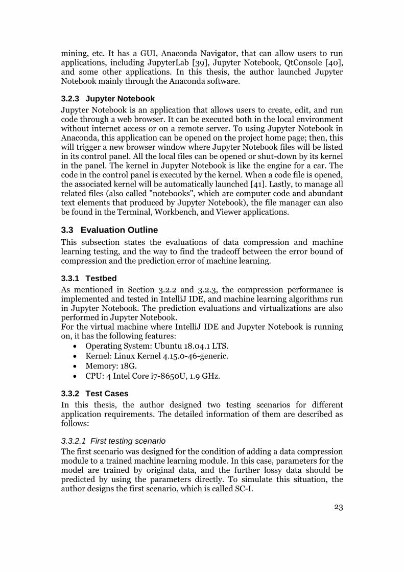
Figure 4.4: Comparison of “outer” convex hulls and “inner” convex hulls
The problem of this new method is that, when we considering the error bound of each point, instead of inputting the real value of this point, the input will be the upper and lower estimates of real value. As Figure 4.4 shows, when 10% error bound is accepted, the input of one point with value a will be (𝑎 + 𝑎 ∗10%) and (𝑎 − 𝑎 ∗ 10%). If we only find the two “outer” hulls of all inputs and insist that a line lay inside two hulls conforms to the error requirement of current compressed points, there will be a problem. In some cases, it might violate the error bound for some compressed points, as shown in the first graph of Figure 4.4. Therefore, instead of generating outer hulls, I build two inner hulls for error-tolerant detection. For the upper hull, I remove the second-to-last point only when there is a clockwise turn. For the lower hull, it is reversed. In this way, it can guarantee that if the best-fit line lies inside the upper and lower hulls, it conforms to the error bound of current compressed points, otherwise restart a new approximation from the break-up point.

33
4.1.2.3 PLA Compression Protocol
The following paragraphs describe how PLA methods are can be used to produce a stream of compressed data multi-dimensional time series data. To deal with time series data with multiple features, one effective method is to compress each feature with an individual channel. For example, a weather monitoring system usually collects different real-time information, including temperature, humidity, water vapor pressure, air density, wind direction, together with the current timestamp. To compress this tupled stream with six features, the way is to fit six features to six independent channels and handle these channels simultaneously. Note that in PLA, timestamps are needed to reconstruct data from best-fit lines. But it increases the cost to record every timestamp than updating a counter during the compression process. By using a counter as the x-axis, we only add the count of compressed data to outputs. Additionally, the timestamps 𝑡𝑖 can also be treated in one individual channel by compressing the tupled stream (𝑖, 𝑡𝑖).
Figure 4.5: OneStream protocol flowchart with multiple input channels
As Figure 4.5 shows, we can have multiple OneStream channels to deal with high dimensional tuples. The OneStream protocol defines a single stream output to PLA decompressor aggregated by multiple streams. The stream of input tuples, e.g. (𝑡𝑖, 𝑦1𝑖 , 𝑦2𝑖)𝑖>0 , is a three-dimensional stream, so each feature is fitted with its serial number to one individual channel and compressed parallelly. These serial numbers indicate the location of data and will be sent along with triplets (a, b, n) for further reconstruction. In this case, n is a counter to count the number of tuples compressed by a line segment, and it is used as a timestamp for each compressed point as well (also for the real timestamp feature). For each channel, it maintains an independent counter. The counter is set to 1 when a new line approximation starts and stops current approximation when it reaches its maximum value (e.g., 256 when 1 byte is used). A pre-determined maximum value for the counter is helpful to control compression delay.

34
There are two central latencies in PLA compression. One is computation latency; the other is data retention latency. PLA compression records are generated adaptively when they have been adequately approximated. Hence, PLA decompressor must always wait for a line segment to reconstruct the compressed records. The reconstruction of values along a line segment is possible as soon as the last point of this line segment is determined. If one feature has an exact linear increasing pattern (e.g., for a timestamp collected every 1 minute), there will be a long delay to wait for the compression records without a counter to terminate it. Set the upper limit of counters might be helpful in reducing reconstruction latencies with the cost of lower compression ratios. Note that there is also a lower limit for counters. As shown in Figure 4.5, the lower limit of counters is 3, which means that we don’t consider the compression records when compressed points are equal or less than 3. Instead, the original values are transmitted to improve the efficiency and accuracy of the compression model. In this situation, serial numbers are set to opposite to inform PLA decompressor that the following values are uncompressed.
4.1.3 PLA Decompressor Module
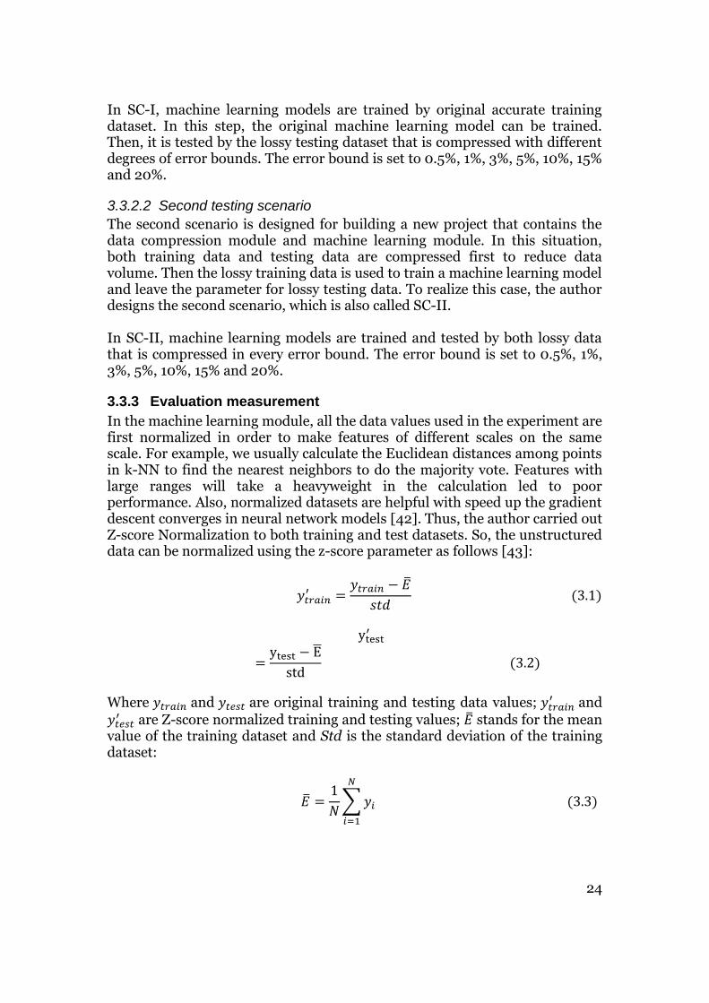
The functions of PLA decompressor are reconstruction and synchronization from input compression stream. This section will present the reconstruction process and how decompressed values will be synchronized and output as the format of original dataset.
4.1.3.1 Reconstruction Process
The reconstruction process of PLA decompressor is quite straight-forward. To reconstruct the input compression stream, the first thing is to check serial numbers. If it is negative, directly output the next records; otherwise, when the serial number is positive and n>3, read the next three coefficients a, b, and n and compute result sequence. The i-th reconstructed record is defined as: 𝑦𝑖
′ = 𝑎 ∗ 𝑖 + 𝑏 𝑖 ∈ (0, 𝑛] (4.12) When n reconstructed tuples are ready, the result is relocated according to its serial number. For example, as Figure 4.6 shows, there are two inputs (1, a, b, 5) and (-3, 𝑦𝑖, 𝑦𝑖+1, 𝑦𝑖+2). To deal with the first input, we check that the serial number is positive and compute the result (0.51, 0.55, 0.62, 0.68, 0.73) using a, b, and the counter n=5. Again, we check serial number is 1, then the reconstructed results belong to the sequence of the first column (e.g., Timestamp) and are appended to the end of the sequence. Next comes (-3, 𝑦𝑖, 𝑦𝑖+1, 𝑦𝑖+2), and values are immediately added to the third column (In Figure 4.6, we assume that 𝑦𝑖 = 10.5, 𝑦𝑖+1 = 21.3, 𝑦𝑖+2 = 33.1). In this pattern, the length of each feature sequence is different due to independent compression channels. However, the time series data (like (𝑡𝑖, 𝑦1𝑖 , 𝑦2𝑖)𝑖>0) is expected to output as soon as it is reconstructed. To output
35
the decompressed data in the original form of (timestamp, feature1, feature2, …), the result need synchronization after the steps of relocation.
Figure 4.6: Structure of PLA Decompressor
4.1.3.2 Synchronization
To realize data synchronization and output time series in real time, PLA decompressor has local counters for each feature and timestamp. For instance, in Figure 4.6, three counters are needed for timestamp, feature 1 and feature 2. Every time there is an input, counters are updated and checked. If the smallest value of counters is n>0, then immediately output the top n collections. As Figure 4.6 shows, the original values of counters are 1, 8, 0 before the input of (1, a, b, 5). Right after the first input (1, a, b, 5) is processed, counters are refreshed to 6, 8, 0, and still no output. When the second input (-3, 𝑦𝑖, 𝑦𝑖+1, 𝑦𝑖+2) is reconstructed, counters change to 6, 8, 3. The smallest value of counters is 3 and the top 3 data is output. On the one hand, use local counters to output data once complete time series data is generated can reduce the latency as much as possible. On the other hand, avoid ineffective compression of fewer than three values can noticeably decrease long latency when the PLA compression has a poor performance.
4.1.4 Machine Learning Module
The machine learning Module is independent of PLA Compressor Module and Decompressor Module. Instead of building in IntelliJ environment as the aforementioned two modules, Machine Learning Module is built in Jupyter notebook using Python language. When the streaming data is reconstructed in PLA decompressor, the data is automatically stored in a local file in real time. Therefore, the data file can be further invoked in Machine Learning Module as the input for all machine learning models. Basically, the author implemented 6 machine learning algorithms for comparison: linear regression, random forest, k-NN, logistic regression, SimpleRNN, and LSTM. Linear regression, logistic regression, random forest, and k-NN are built using scikit-learn [48] library, whereas using Keras [49] library for RNN and LSTM.
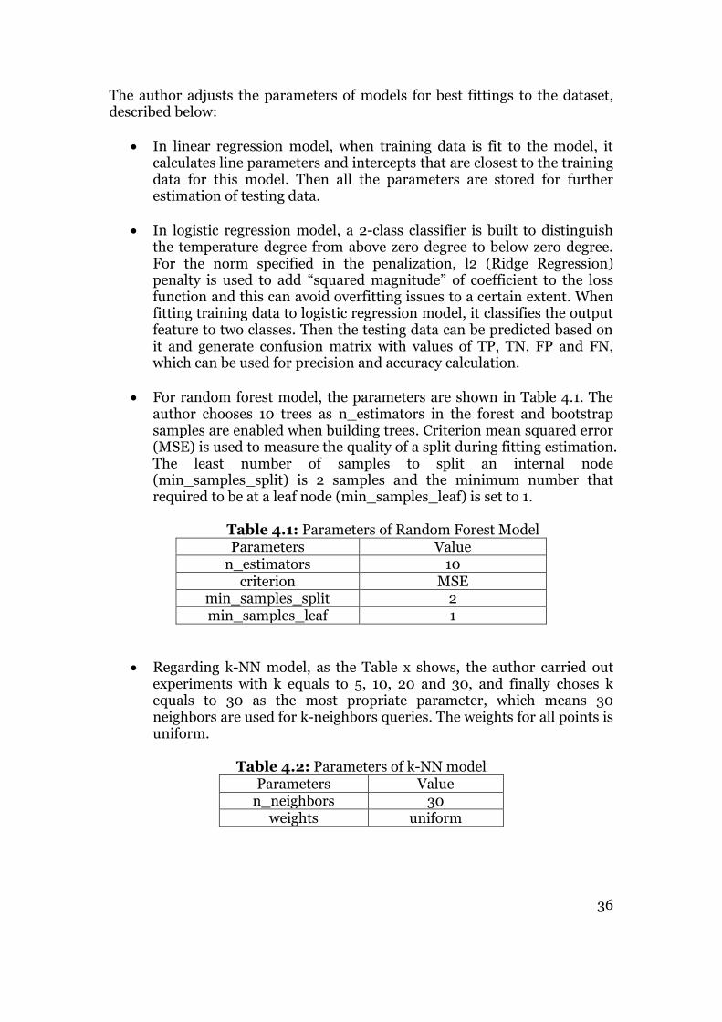
36
The author adjusts the parameters of models for best fittings to the dataset, described below:
• In linear regression model, when training data is fit to the model, it calculates line parameters and intercepts that are closest to the training data for this model. Then all the parameters are stored for further estimation of testing data.
• In logistic regression model, a 2-class classifier is built to distinguish the temperature degree from above zero degree to below zero degree. For the norm specified in the penalization, l2 (Ridge Regression) penalty is used to add “squared magnitude” of coefficient to the loss function and this can avoid overfitting issues to a certain extent. When fitting training data to logistic regression model, it classifies the output feature to two classes. Then the testing data can be predicted based on it and generate confusion matrix with values of TP, TN, FP and FN, which can be used for precision and accuracy calculation.
• For random forest model, the parameters are shown in Table 4.1. The author chooses 10 trees as n_estimators in the forest and bootstrap samples are enabled when building trees. Criterion mean squared error (MSE) is used to measure the quality of a split during fitting estimation. The least number of samples to split an internal node (min_samples_split) is 2 samples and the minimum number that required to be at a leaf node (min_samples_leaf) is set to 1.
Table 4.1: Parameters of Random Forest Model Parameters Value
n_estimators 10 criterion MSE
min_samples_split 2 min_samples_leaf 1
• Regarding k-NN model, as the Table x shows, the author carried out experiments with k equals to 5, 10, 20 and 30, and finally choses k equals to 30 as the most propriate parameter, which means 30 neighbors are used for k-neighbors queries. The weights for all points is uniform.
Table 4.2: Parameters of k-NN model
Parameters Value n_neighbors 30
weights uniform

37
Figure 4.7: Layer Structure of RNN Model
• For RNN, as Figure 4.7 shows, the model is built with 1 input layer, 2 hidden SimpleRNN layers and 1 dense layer as the output layer. The author mainly focusses on adjusting the parameters described in Table 4.3. Except for input layer, three layers are used including two SimpleRNN and one Dense. The author did tests on RNN models with 1 and 3 SimpleRNN layers as well. But an RNN model with one SimpleRNN layer has a higher error in which three SimpleRNN layers cause low effectiveness. For regulation, the author chooses Dropout and Recurrent Dropout to ignore arbitrary units during training process to avoid overfitting situations. These 2 parameters are set to 0.3, which means 30% of units in a SimpleRNN layer are randomly dropped out. To compile RNN model, an optimizer is required. By testing the most popular optimizer RMSprop and Adam, the author found RMSprop with has a better performance. The learning rate is also a parameter to control the training and avoid overfitting. The best learning rate tested is 0.0005 in this case, which makes predictions reach the lowest error.
Table 4.3: Parameters of RNN model
Parameters Value Layer 3 Cell SimpleRNN
Regulation Dropout: 0.3 Recurrent Dropout: 0.3

38
Optimizer RMSprop Learning Rate 0.0005
Figure 4.8: Layer Structure of LSTM Model
• Regarding LSTM, it has a similar layer structure as RNN but with LSTM cells in hidden layers, as Figure 4.8 shows. Also, LSTM model is built with similar parameters as RNN model. The only difference is the learning rate is 0.0001, which is smaller than RNN. So, it has more iterations and can usually get a better result. Table 4.4 gives the detail information of parameter adjusting for LSTM model.
Table 4.4: Parameters of LSTM model Parameters Value
Layer 3 Cell LSTM
Regulation Dropout: 0.3 Recurrent Dropout: 0.3
Optimizer RMSprop Learning Rate 0.0001
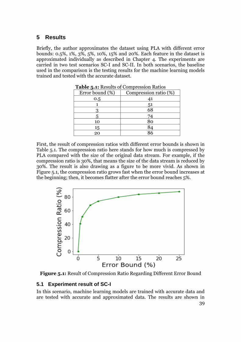
39
5 Results
Briefly, the author approximates the dataset using PLA with different error bounds: 0.5%, 1%, 3%, 5%, 10%, 15% and 20%. Each feature in the dataset is approximated individually as described in Chapter 4. The experiments are carried in two test scenarios SC-I and SC-II. In both scenarios, the baseline used in the comparison is the testing results for the machine learning models trained and tested with the accurate dataset.
Table 5.1: Results of Compression Ratios Error bound (%) Compression ratio (%)
0.5 41 1 51 3 68 5 74
10 80 15 84 20 86
First, the result of compression ratios with different error bounds is shown in Table 5.1. The compression ratio here stands for how much is compressed by PLA compared with the size of the original data stream. For example, if the compression ratio is 30%, that means the size of the data stream is reduced by 30%. The result is also drawing as a figure to be more vivid. As shown in Figure 5.1, the compression ratio grows fast when the error bound increases at the beginning; then, it becomes flatter after the error bound reaches 5%.
Figure 5.1: Result of Compression Ratio Regarding Different Error Bound
5.1 Experiment result of SC-I
In this scenario, machine learning models are trained with accurate data and are tested with accurate and approximated data. The results are shown in

40
Figure 5.2, 5.4 and 5.6. Specifically, Figure 5.2 shows the results of linear regression, k-NN and random forest. Note that the models perform very well when the error bound is 0, meaning that when there is no data approximation, the models can give perfect predictions.
Figure 5.2: Experiment Results of SC-I: Normalized MAE of Linear
Regression, Random Forest and k-NN
• Impact of data compression to linear regression We can see that the normalized MAE is quickly increased to 0.2, after that it becomes quite flat. The growth of normalized MAE is quite similar to the growth of the compression ratio when the error bound increases. Though linear regression is sensitive to the data approximation when the error bound is under 5%, but it still performs very well: The standard deviation of temperature in the dataset is 8.4, when the normalized MAE is 0.2, the average prediction error is 1.68°C, given that the compression ratio is 74%. To further explain the results, the behavior of linear regression can be considered. Linear regression always takes a global view of statistics over the whole dataset. The “best-fit line" is gotten from finding the optimal model parameters towards the global minimum of the cost function. Therefore, when there is any deviation, the testing data will be dispersed from the “best-fit line" which leads to a higher MAE.

41
Figure 5.3: Trend of Error Changing with 0%, 10% and 20% Error Bounds in
Linear Regression
Figure 5.3 shows scatter plots of linear regression, which indicates the general trend of prediction error changing with error bounds. The black line is the regression fit line, which means that the estimated values lie on the black line just equal to real values. The yellow points are prediction errors with estimated values on x-axis and real values on y-axis. Therefore, the more yellow scatters are closed to the black line, the less prediction error is. The scatter plots illustrate that, as the error bound increases, points become more scattered, so the prediction error increase as well.
• Impact of data compression to k-NN From Figure 5.2, we see that k-NN performs better than linear regression, which only has a slight increase at the early stage and a prolonged growth later. The normalized MAE increases to around 0.075 when the error bound is 20%, which means the average prediction error goes up from 0.13˚C (when the error bound is 0) to 0.7˚C, with 86% compression ratio. If we compare linear regression and k-NN, we can find that unlike linear regression, k-NN is much more sensitive to the local structure of

42
the dataset. When a testing data point deviates from its original value, it may cause its location to change in the feature space, but it may still has the same neighbors. Furthermore, even if some of its neighbors change, the corresponding prediction results may still not change significantly since it is calculated as the average value of the k nearest neighbors.
• Impact of data compression to random forest Regarding the performance of random forest, the normalized MAE has a small but sustained growth with the growth of error bound. The normalized MAE increases to 0.09 when the error bound is 20%, which means the average prediction error rises from 0.002˚C to 0.84˚C. The characteristic of a random forest model is that it takes the mean values of multiple decision trees as the output. Due to randomness enhancement of bagging, random forest has some anti-noise ability. However, the compression of testing data still has chances to impact the outputs of decision trees. Each decision tree in the random forest is a binary tree when the data deviation can influence the branching, it will change the corresponding output, even if the deviation is small.
• Impact of data compression to logistic regression
Figure 5.4: Experiment Results of SC-I: Normalized MAE of Logistic
Regression Figure 5.4 shows the performance of logistic regression. This diagram shows that the tendency of normalized MAE growth is similar to that of linear regression. That is because logistic regression is also trying to find optimal model parameters towards the global minimum of the cost function. Compared to linear regression, logistic regression is less sensitive to approximated testing data. The normalized MAE of logistic

43
regression is round 0.05 when error bound is 20%, which is far less than linear regression. The reason is that logistic regression classifies whether the output is positive or negative by using the sigmoid function
𝑠𝑖𝑔(𝑡) =1
1+𝑒−𝑡 . If sig(t) is more significant than 0.5, the prediction
result will become 1 and if sig(t) is smaller than 0.5, the prediction result will become 0. In this case, only the deviation of the data that maps to around 0.5 may affect the prediction outputs, while others will still lead to the same outputs. Therefore, logistic regression is much more stable with the impact of data compression. The shortcoming is obvious: logistic regression can only model several classes of events.
• Impact of data compression to RNN and LSTM To test the performance of RNN and LSTM, the author forecast future temperatures of one day using statistics from history ten days, which cannot be done with the four methods above. The training results of RNN and LSTM models are shown in Figure 5.5. By adjusting dropout, learning rate and other parameters, training loss is similar to validation loss, which means that the model trains well without overfitting and underfitting.
Figure 5.5: (a) Training Process of RNN Model. The Num. of Epochs Is 35; (b) Training Process of LSTM Model. The Num. of Epochs Is 30.
The results of prediction error of RNN and LSTM models are shown in Figure 5.6. When the error bound is 20%, the normalized MAE is 0.31 for SimpleRNN and 0.285 for LSTM model. Note that the normalized MAE for the baseline scenario (error bound is 0) is 0.28; the impact of data approximation to RNN and LSTM is quite small. More specifically, SimpleRNN only increases the average prediction error by 0.24˚C when error bound is 20% compared with the baseline. LSTM performs even better. Since the dropout is introduced in both RNN and LSTM models, by randomly dropping some features in the hidden layers, it improves the robustness of those models, which improves the stability of those models to inaccurate data. LSTM has better robustness than
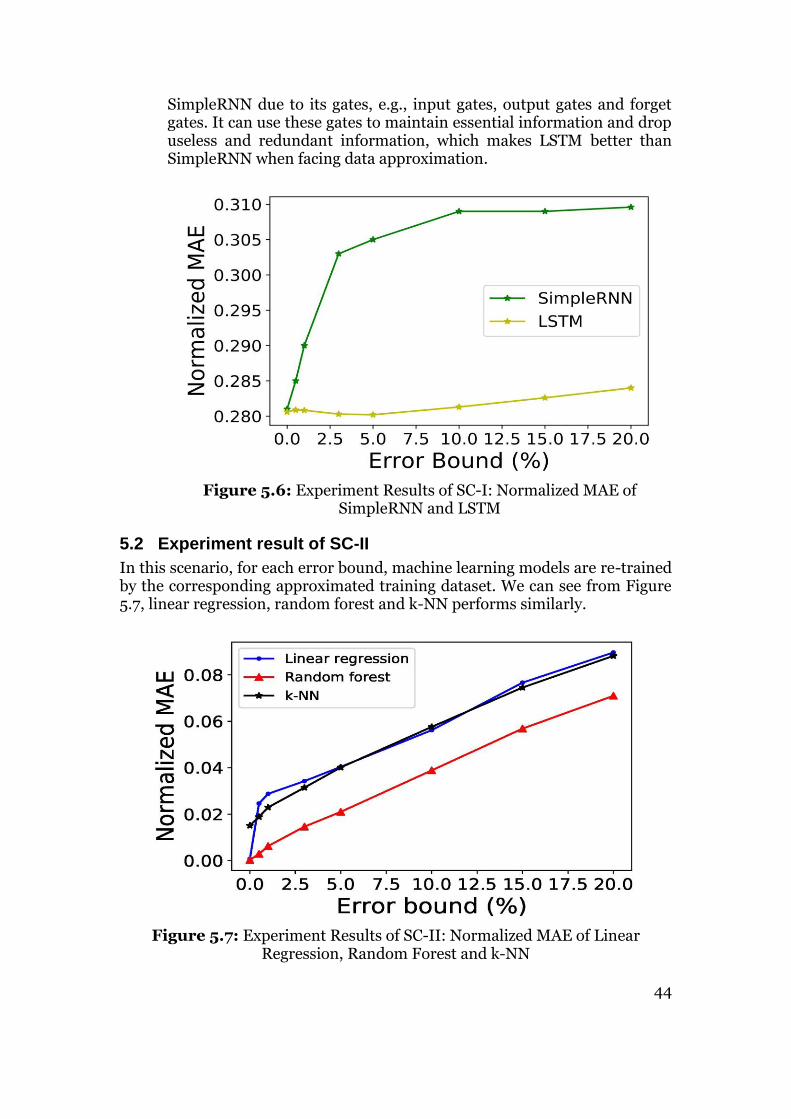
44
SimpleRNN due to its gates, e.g., input gates, output gates and forget gates. It can use these gates to maintain essential information and drop useless and redundant information, which makes LSTM better than SimpleRNN when facing data approximation.
Figure 5.6: Experiment Results of SC-I: Normalized MAE of
SimpleRNN and LSTM
5.2 Experiment result of SC-II
In this scenario, for each error bound, machine learning models are re-trained by the corresponding approximated training dataset. We can see from Figure 5.7, linear regression, random forest and k-NN performs similarly.
Figure 5.7: Experiment Results of SC-II: Normalized MAE of Linear
Regression, Random Forest and k-NN

45
In Figure 5.7, the corresponding normalized MAEs all have a roughly linear growth when the error bound increases. In particular, the normalized MAE increases to 0.09 for linear regression, 0.079 for k-NN and 0.073 for random forest, which is quite close. The reason for the linear growth of normalized MAE is two-folded: on the one hand, the machine learning models are trained and tested by the corresponding approximated datasets; on the other hand, the prediction error is calculated by comparing the predicted values to the real observed values. Therefore, what the figure shows is actually the difference between the models for approximated datasets and the models for the original dataset. The difference should have linear relationship with the error bound.
Figure 5.8: Experiment Results of SC-II: Normalized MAE of Logistic
Regression
However, in Figure 5.8, it is interesting to see that logistic regression behaves similarly as it behaves in scenario SC-I. Comparing the error in SC-I that increased 0.04, logistic model has a similar increase error of 0.035 in SC-II. To analyze it, the author thinks this is due to the principle of logistic regression. Only the data points that are mapped near the demarcation may be influenced due to the approximation. So even with different training datasets, only a few data that close to the boundary line will be influenced, but no significant difference in two test scenarios.

46
Figure 5.9: Experiment Results of SC-II: Normalized MAE of SimpleRNN
and LSTM
Figure 5.9 shows the performance of SimpleRNN and LSTM in scenario SC-II. We can see that the normalized MAEs fluctuates, but within a small range, for both SimpleRNN and LSTM. This thanks to the excellent robustness of RNN and LSTM. The fluctuation may be caused by the randomness of each training process using inaccurate datasets. Again, as in scenario SC-I, we see good robustness and forecasting performance to approximated data for both SimpleRNN and LSTM. To summarize, linear regression, k-NN and random forest behave differently in scenarios SC-I and SC-II. In both scenarios, most of the time, random forest performs better than the other two. Logistic regression behaves similarly in both scenarios. SimpleRNN and LSTM demonstrate good robustness and forecasting performance with data approximations.

47
6 Conclusions
In this paper, the author investigates the impact of data approximation to multiple popular machine learning methods by analyzing two test scenarios on a typical time series. The inaccurate testing dataset is used to test the performance of machine learning models trained with the accurate dataset and inaccurate dataset. In the first test scenario where machine learning models are trained with accurate datasets and tested by datasets with different compression error bounds, in traditional supervised learning, linear regression has the worst performance while random forest and k-NN performs well. Due to the principle of logistic regression, it also has excellent stability. The first test scenario can be applied in the situation that engineers want to apply compression to future data collecting and fit the data to an existing well-trained model. In the second test scenario, the results show the common linear growth trend on linear regression, random forest and k-NN. But random forest performs better than the other two. In addition, there is no significant difference in logistic regression with different test scenarios. For RNN and LSTM models, they are more stable in the second test scenario. This test scenario can be referenced to the application when engineers want to compress data and use it to train a machine learning model. From the experiment results, the advantage of using data approximation in transferring big data streams is: it can dramatically reduce the volume of data needed to be transferred while keeping the impact on the machine learning applications quite small. Also, there is a trade-off among error bound, compression ratio and prediction accuracy. The contributions of this thesis are: First, it improved the traditional PLA method to make it more adaptive and flexible when dealing with multi-dimensional time series data. Second, it designed two test scenarios to study the influence of machine learning with an approximation on time series. It tested the most popular machine learning algorithms with different principles, including mathematical statistics, cluster analysis, tree type, neural network and so on. Third, it is reasonable to believe that the finding can provide useful guidelines for real deployments of data collections in various use cases, e.g., massive IoT, V2X and industrial automation. For future guides, if engineers want to compress time series data to save transmission bandwidth and storage space, the author recommends engineers to choose PLA compression with an error bound in the range of (0, 5%] together with random forest model for time series regression problems. Also, we find that LSTM model has an outstanding performance compared with RNN. So, for the time series forecasting problem, LSTM is better in this situation.
6.1 Future work
Regarding future work, the following aspects are worth considering:
• Apply more time series data to find if there is a common trend for different types of time series.

48
• Build more machine learning models. So far, the tests are limited to several machine learning algorithms because of time. In the future, the author would like to test more advanced machine learning models to make a guide for more real-world applications.
• Consider feature selection both on compression and machine learning. For PLA compression, it can add weights to different features. Less essential features should get lower weights and been compressed to smaller sizes, while important features can keep more information. Using this method may reduce prediction errors in machine learning. For machine learning applications, it can also add feature selection to filter out less essential features. In this way, the influence of compression on machine learning may be further decreased.
• Finally, it would be interesting to use reinforcement learning to have an optimal choice of error bounds.

49
7 References
[1] Shumway, Robert H.; Stoffer, David S,;, Time Series Analysis and Its Applications, Springer, 2017.
[2] Liang, Xin; Di, Sheng; Tao, Dingwen; Li, Sihuan; Li, Shaomeng; Guo, Hanqi; Chen, Zizhong; Cappello, Franck, "Error-controlled lossy compression optimized for high compression ratios of scientific datasets," 2018 IEEE International Conference on Big Data (Big Data), pp. 438-447, 2018.
[3] Saud, NAQVI; Rameez, NAQVI; RIAZ, Raja Ali; Faisal, SIDDIQUI, "Optimized RTL design and implementation of LZW algorithm for high bandwidth applications," Electrical Review, pp. 279-285, 2011.
[4] Cormen, Thomas H.; Leiserson, Charles E.; Rivest, Ronald L.; Stein, Clifford;, Introduction to Algorithms, MIT Press, 1990, p. 1312.
[5] A. T. Welch, "A Technique for High-Performance Data Compression," Computer, vol. 17, no. 6, pp. 8-19, 1984.
[6] E. C. Shannon, "A Mathematical Theory of Communication," Bell System Technical Journal, vol. 27, pp. 379-423, 1948.
[7] Lin Jessica; Keogh Eamonn; Lonardi Stefano; Chiu Bill, "A symbolic Representation of Time Series, with Implications for Streaming Algorithm," Proceedings of the 8th ACM SIGMOD workshop on Research issues in data mining and knowledge discovery, pp. 2-11, 2003.
[8] C. M. Bishop, Pattern Recognition and Machine Learning, springer, 2006.
[9] Luo, Ge; Yi, Ke; Cheng, Siu-Wing; Li, Zhenguo; Fan, Wei; He, Cheng; Mu, Yadong;, "Piecewise linear approximation of streaming time series data with max-error guarantees," 2015 IEEE 31st International Conference on Data Engineering, p. 173/184, 2015.
[10] Teerapittayanon, Surat; McDanel, Bradley; Kung, Hsiang-Tsung;, "Distributed deep neural networks over the cloud, the edge and end devices.," 2017 IEEE 37th International Conference on Distributed Computing Systems (ICDCS)., pp. 328-339, 2017.
[11] Bastian, Havers; Duvignau, Romaric; Najdataei, Hannaneh; Gulisano, Vincenzo; Koppisetty, Ashok Chaitanya; Papatriantafilou, Marina;, "DRIVEN: a framework for efficient Data Retrieval and clusterIng in VEhicular Networks.," 2019 IEEE 35th International Conference on Data Engineering (ICDE), pp. 1850-1861, 2019.
[12] Faloutsos, Christos; Mudumbai, Ranganathan; Yannis , Manolopoulos;, "Fast subsequence matching in time-series databases," ACM, vol. 23, pp. 419-429, 1994.
[13] Chakrabarti, Kaushik; Keogh, Eamonn; Mehrotra, Sharad; Pazzani, Michael;, "Locally adaptive dimensionality reduction for indexing large time series databases," ACM Transactions on Database Systems (TODS), vol. 27, no. 2, pp. 188-228, 2002.

50
[14] Denegri-Knott, Janice, Mark Tadajewski, "The emergence of MP3 technology," Journal of Historical Research in Marketing 2.4, pp. 397-425, 2010.
[15] D. Austerberry, "The technology of video and audio streaming," Focal Press, 2013.
[16] Pennebaker, William B.; Mitchell, Joan L.;, JPEG: Still Image Data Compression Standard (3rd ed.), Springer, 1993.
[17] Cabrita, Daniel Mealha; Godoy, Walter;, "PNG Optimization Techniques Applied to Lossless Web Images," IEEE Latin America Transactions, vol. 10, no. 1, pp. 1398-1401, 2012.
[18] J. Duda, "Asymmetric numeral systems: entropy coding combining speed of Huffman coding with compression rate of arithmetic coding," arXiv preprint arXiv: 1311.2540, 2013.
[19] Duda, Jarek; Tahboub, Khalid; Gadgil, Neeraj J.; Delp, Edward J.;, "The use of asymmetric numeral systems as an accurate replacement for Huffman coding," 2015 Picture Coding Symposium (PCS), pp. 65-69, 2015.
[20] D. A. Huffman, "A method for the construction of minimum-redundancy codes," Proceedings of the IRE, vol. 40, no. 9, pp. 1098-1101, 1952.
[21] J. S. Vitter, "Design and analysis of dynamic Huffman codes," Journal of the ACM (JACM), vol. 34, no. 4, pp. 825-845, 1987.
[22] Larmore, Lawrence L.; Hirschberg, Daniel S.;, "A fast algorithm for optimal length-limited Huffman codes," Journal of the ACM (JACM), vol. 37, no. 3, pp. 464-473, 1990.
[23] Witten, Ian H.; Neal, Radford M.; Cleary, John G;, "Arithmetic Coding for Data Compression," Communications of the ACM, vol. 30, no. 6, pp. 520-540, 1987.
[24] Larsen, Richard J.; Marx, Morris L.;, An introduction to mathematical statistics and its applications., Englewood Cliffs, NJ: Prentice-Hall, 1986.
[25] Duvignau, Romaric; Gulisano, Vincenzo; Papatriantafilou, Marina; Savic, Vladimir;, "Piecewise Linear Approximation in Data Streaming: Algorithmic Implementations and Experimental Analysis," arXiv preprint arXiv:1808.08877, 2018.
[26] Hastie, Trevor, Robert Tibshirani, Friedman, Jerome, "The Elements of Statistical Learning: Data mining, Inference, and Prediction," New York: Springer, pp. 485-586, 2009.
[27] E. Forgy, "Cluster analysis of multivariate data: efficiency versus interpretability of classifications," Biometrics, vol. 3, no. 21, pp. 768-769, 1965.
[28] Yan, Xin; Xiaogang, Su;, Linear regression analysis: theory and computing, World Scientific, 2009.
[29] J. . Cramer, "The Origins of Logistic Regression," Social Science Research Network, vol. , no. , p. , 2002.
[30] M. E. Maron, "Automatic Indexing: An Experimental Inquiry," Journal of the ACM, vol. 8, no. 3, pp. 404-417, 1961.

51
[31] W.-Y. . Loh, "Classification and regression trees," Wiley Interdisciplinary Reviews-Data Mining and Knowledge Discovery, vol. 1, no. 1, pp. 14-23, 2011.
[32] N. S. Altman, "An introduction to kernel and nearest-neighbor nonparametric regression.," The American Statistician, vol. 3, no. 46, pp. 175-185, 1992.
[33] Han, Jun; Moraga, Claudio;, "The influence of the sigmoid function parameters on the speed of backpropagation learning.," International Workshop on Artificial Neural Networks, pp. 195-201, 1995.
[34] T. K. Ho, "Random decision forests," Proceedings of 3rd International Conference on Document Analysis and Recognition, vol. 1, pp. 278-282, 1995.
[35] Williams, Ronald J.; Hinton, Geoffrey E.; Rumelhart, David E., "Learning representations by back-propagating errors," Nature, vol. 323, no. 6088, pp. 533-536, 1986.
[36] Hochreiter, Sepp; Schmidhuber, Jürgen;, "Long short-term memory," Neural computation, vol. 9, no. 8, pp. 1735-1780, 1997.
[37] Kluyver, Thomas; Ragan-Kelley, Benjamin; Pérez, Fernando; Granger, Brian; Bussonnier, Matthias; Frederic, Jonathan; Kelley, Kyle; Hamrick, Jessica; Grout, Jason; Corlay, Sylvain; Ivanov, Paul; Avila, Damián; Abdalla, Safia; Willing, Carol; Jupyter Developmet, "Jupyter Notebooks-a publishing format for reproducible computational workflows.," ELPUB, pp. 87-90, 2016.
[38] A. S. Distribution, "ANACONDA," Anaconda, Inc., November 2016. [Online]. Available: https://anaconda.com. [Accessed August 2019].
[39] P. Jupyter, "JupyterLab is Ready for Users," 20 February 2018. [Online]. Available: https://blog.jupyter.org/jupyterlab-is-ready-for-users-5a6f039b8906. [Accessed 1 August 2019].
[40] T. J. D. Team, "Jupyter Qt Console," [Online]. Available: https://qtconsole.readthedocs.io/en/latest/. [Accessed August 2019].
[41] A. I. a. contributors, "What is the Jupyter Notebook?," 2015. [Online]. Available: https://jupyter-notebook-beginner-guide.readthedocs.io/en/latest/what_is_jupyter.html. [Accessed 1 August 2019].
[42] Ioffe, Sergey; Szegedy, Christian;, "Batch normalization: Accelerating deep network training by reducing internal covariate shift.," arXiv preprint arXiv:1502.03167, 2015.
[43] Zill, Dennis; Wright, Warren S; Cullen, Michael R;, "Advanced engineering mathematics.," Jones & Bartlett Learning., 2011.
[44] N. Ketkar, Deep Learning with Python, Apress, 2017.
[45] O. Kolle, "Max-Planck-Institute for Biogeochemistry, Jena," Max-Planck-Institute for Biogeochemistry, [Online]. Available: https://www.bgc-jena.mpg.de/wetter/. [Accessed 01 06 2019].
[46] S. J. Miller, "The method of least squares.," Mathematics Department Brown University, no. 114, 2006.

52
[47] R. L. Graham, "An Efficient Algorithm for Determining the Convex Hull of a Finite Planar Set," Inf. Process. Lett., vol. 1, pp. 132-133, 1972.
[48] Pedregosa, F.; Varoquaux, G.; Gramfort, A.; Michel, V.; Thirion, B.; Grisel, O.; Blondel, M.; Prettenhofer, P.; Weiss, R.; Dubourg, V.; Vanderplas, J.; Passos, A.; Cournapeau, D.; Brucher, M.; Perrot, M.; Duchesnay, E.;, "Scikit-learn: Machine Learning in Python," Journal of Machine Learning Research, vol. 12, pp. 2825--2830, 2011.
[49] Chollet, Francois; others;, "Keras," 2015. [Online]. Available: https://keras.io. [Accessed 01 09 2019].

1

TRITA-EECS-EX-2019:786