experimental wave effects on vertical relative …
TRANSCRIPT
EXPERIMENTAL WAVE EFFECTS ON VERTICAL RELATIVE MOTION
A Thesis
by
RAJITH PADMANABHAN
Submitted to the Office of Graduate Studies ofTexas A&M University
in partial fulfillment of the requirements for the degree of
MASTER OF SCIENCE
May 2006
Major Subject: Ocean Engineering
EXPERIMENTAL WAVE EFFECTS ON VERTICAL RELATIVE MOTION
A Thesis
by
RAJITH PADMANABHAN
Submitted to the Office of Graduate Studies ofTexas A&M University
in partial fulfillment of the requirements for the degree of
MASTER OF SCIENCE
Approved by:
Chair of Committee, Cheung Hun KimCommittee Members, Moo-Hyun “Joseph” Kim
Achim StosselHead of Department, David V Rosowsky
May 2006
Major Subject: Ocean Engineering
iii
ABSTRACT
Experimental Wave Effects on Vertical Relative Motion. (May 2006)
Rajith Padmanabhan, B.Tech., Cochin University of Science and Technology
Chair of Advisory Committee: Dr. Cheung Hun Kim
Ship motions are influenced by the sea state. Conventionally the responses are
calculated in the frequency domain. This method, however, is valid only for narrow
band spectra. As the seaway becomes more nonlinear, the ship motions cannot be
readily predicted using the spectral method. Experiments conducted by Dalzell, have
shown that the Response Amplitude Operator (RAO) decreased with increasing sea
state or non linearity. Conventionally in the shipbuilding industry, the ship motions
are studied by the linear RAOs and the energy density spectrum of the seaway. This
method does not take into consideration any non linearities in the system. These
are ignored and the ship seaway system is modeled linearly. The following work
analyzes ship motions in the conventional linear approach and compares it to time
domain simulations using the technique outlined in the work, viz. UNIOM (Universal
Nonlinear Input Output Method). Time domain simulation of the SL-7 container ship
hull is carried out. A comparison of the most probable peak value of the different
modes of motion indicates that the linear theory tends to overpredict.

iv
To Amma and Sampada
v
ACKNOWLEDGMENTS
This research was conducted at Texas A&M University with the support of the
Department of Civil Engineering, through the Texas Engineering Experiment Station
(TEEX). I wish to thank my chair, Dr. C.H.Kim, for his valuable contribution toward
this thesis and for having shared with me his valuable insights in the field of Naval
Architecture, Hydrodynamics and Statistics. I wish to thank Dr. M.H.Kim and
Dr. Achim Stossel for their guidance throughout this research project. I wish to
thank Adam Adil (Exmar Offshore) for having helped me out with the programs
and Mr. Jeffery Arthur Richer (US Navy) for his support throughout this research
work. For all things related to the use of the computer, from installing the hardware
to debugging code and finally typesetting the whole work in LATEX, my good friend
Thomas has most patiently listened to and helped me solve every issue in the nick
of time. I thank him for his patience and wholehearted support. I am indebted
to my classmates, Mr. Basil Theckumpurath and Ms.Amal Chellappan, for their
constant support and motivation. Special thanks to my family for their faith in me
and constantly motivating me, without them I would not have been able to come this
far.
vi
TABLE OF CONTENTS
CHAPTER Page
I INTRODUCTION . . . . . . . . . . . . . . . . . . . . . . . . . . . 1
1. Motivation . . . . . . . . . . . . . . . . . . . . . . . . . . . . . 1
1.1. Motivation . . . . . . . . . . . . . . . . . . . . . . . . . 2
1.2. Application . . . . . . . . . . . . . . . . . . . . . . . . 3
2. Approach . . . . . . . . . . . . . . . . . . . . . . . . . . . . . 4
2.1. Linear and Nonlinear Model . . . . . . . . . . . . . . . 4
II THE UNIOM MODEL . . . . . . . . . . . . . . . . . . . . . . . . 5
1. Strip Theory . . . . . . . . . . . . . . . . . . . . . . . . . . . 5
2. Equations of Motion . . . . . . . . . . . . . . . . . . . . . . . 6
3. The Ship Motion Program . . . . . . . . . . . . . . . . . . . . 9
3.1. Ship Particulars . . . . . . . . . . . . . . . . . . . . . . 9
4. Input Waves . . . . . . . . . . . . . . . . . . . . . . . . . . . . 10
4.1. Froude Similitude Law . . . . . . . . . . . . . . . . . . 11
4.2. The Modified JONSWAP Spectrum . . . . . . . . . . . 12
4.3. ITTC Spectrum . . . . . . . . . . . . . . . . . . . . . . 13
4.4. Encounter Frequency Domain . . . . . . . . . . . . . . 13
5. KRISO Data Analysis . . . . . . . . . . . . . . . . . . . . . . 14
6. Response Analysis . . . . . . . . . . . . . . . . . . . . . . . . 14
7. Spectral Response Analysis . . . . . . . . . . . . . . . . . . . 14
8. Zero Crossing Analysis . . . . . . . . . . . . . . . . . . . . . . 17
9. Probability of Exceedence . . . . . . . . . . . . . . . . . . . . 17
10. Most Probable Peak Analysis . . . . . . . . . . . . . . . . . . 17
III SHIP MOTION CALCULATION . . . . . . . . . . . . . . . . . . 19
1. Input Wave Spectra . . . . . . . . . . . . . . . . . . . . . . . . 19
2. Linear Transfer Function or RAO . . . . . . . . . . . . . . . . 19
3. Response Amplitude Operator . . . . . . . . . . . . . . . . . . 20
3.1. Heading=90o, Froude number=0.00 . . . . . . . . . . . 20
3.2. Heading=90o, Froude number=0.15 . . . . . . . . . . . 20
3.3. Heading=135o, Froude number=0.00 . . . . . . . . . . 22
3.4. Heading=135o, Froude number=0.15 . . . . . . . . . . 22
4. Results from the Linear Method and UNIOM . . . . . . . . . 22
IV ANALYSIS RESULTS FOR HEADING = 90O AND FN = 0.00 . 28
vii
CHAPTER Page
1. Simulation Results . . . . . . . . . . . . . . . . . . . . . . . . 28
2. Probability of Exceedence . . . . . . . . . . . . . . . . . . . . 28
2.1. Case 1 Hs = 3.0m . . . . . . . . . . . . . . . . . . . . . 28
2.2. Case 2 Hs = 4.0m . . . . . . . . . . . . . . . . . . . . . 31
2.3. Case 3 Hs = 6.0m . . . . . . . . . . . . . . . . . . . . . 39
2.4. Case 4 Hs = 7.0m . . . . . . . . . . . . . . . . . . . . . 44
2.5. Case 5 Hs = 9.0m . . . . . . . . . . . . . . . . . . . . . 49
2.6. Case 6 Hs = 11.0m . . . . . . . . . . . . . . . . . . . . 54
3. Most Probable Peak Value . . . . . . . . . . . . . . . . . . . . 54
4. Inference of Results . . . . . . . . . . . . . . . . . . . . . . . . 60
V ANALYSIS RESULTS FOR HEADING = 135O AND FN =
0.15 . . . . . . . . . . . . . . . . . . . . . . . . . . . . . . . . . . 61
1. Simulation Results . . . . . . . . . . . . . . . . . . . . . . . . 61
2. Probability of Exceedence . . . . . . . . . . . . . . . . . . . . 61
2.1. Case 1 Hs = 3.0m . . . . . . . . . . . . . . . . . . . . . 61
2.2. Case 2 Hs = 4.0m . . . . . . . . . . . . . . . . . . . . . 64
2.3. Case 3 Hs = 6.0m . . . . . . . . . . . . . . . . . . . . . 72
2.4. Case 4 Hs = 7.0m . . . . . . . . . . . . . . . . . . . . . 77
2.5. Case 5 Hs = 9.0m . . . . . . . . . . . . . . . . . . . . . 82
2.6. Case 6 Hs = 11.0m . . . . . . . . . . . . . . . . . . . . 87
3. Most Probable Peak Value . . . . . . . . . . . . . . . . . . . . 87
VI ANALYSIS RESULTS FOR HEADING = 180O AND FN = 0 . . 94
1. Simulation Results . . . . . . . . . . . . . . . . . . . . . . . . 94
2. Probability of Exceedence . . . . . . . . . . . . . . . . . . . . 94
2.1. Case 1 Hs = 3.0m . . . . . . . . . . . . . . . . . . . . . 94
2.2. Case 2 Hs = 4.0m . . . . . . . . . . . . . . . . . . . . . 96
2.3. Case 3 Hs = 6.0m . . . . . . . . . . . . . . . . . . . . . 101
2.4. Case 4 Hs = 7.0m . . . . . . . . . . . . . . . . . . . . . 106
2.5. Case 5 Hs = 9.0m . . . . . . . . . . . . . . . . . . . . . 110
2.6. Case 6 Hs = 11.0m . . . . . . . . . . . . . . . . . . . . 114
3. Most Probable Peak Value . . . . . . . . . . . . . . . . . . . . 114
VII SUMMARY OF ANALYSIS RESULTS . . . . . . . . . . . . . . . 119
1. Analysis Results for Heading = 135o AND Fn = 0.00 . . . . . 119
2. Analysis Results for Heading = 180o AND Fn = 0.15 . . . . . 119
3. Observation . . . . . . . . . . . . . . . . . . . . . . . . . . . . 119

viii
CHAPTER Page
VIII CONCLUSION . . . . . . . . . . . . . . . . . . . . . . . . . . . . . 122
REFERENCES . . . . . . . . . . . . . . . . . . . . . . . . . . . . . . . . . . 124
VITA . . . . . . . . . . . . . . . . . . . . . . . . . . . . . . . . . . . . . . . . 125
ix
LIST OF TABLES
TABLE Page
1 Main particulars of the SL 7 containership . . . . . . . . . . . . . . . 10
2 KRISO experimental wave specification . . . . . . . . . . . . . . . . 12
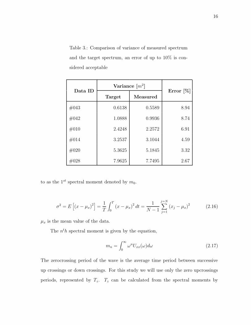
3 Comparison of variance of measured spectrum and the target spec-
trum, an error of up to 10% is considered acceptable . . . . . . . . . 16
x
LIST OF FIGURES
FIGURE Page
1 Pitch transfer RAO from Dalzell’s experiment [source: (Cummins 1973)] 2
2 The UNIOM model . . . . . . . . . . . . . . . . . . . . . . . . . . . . 5
3 Sketch of oblique wave trains incident on a ship [source: (Kim C
H, 2006)] . . . . . . . . . . . . . . . . . . . . . . . . . . . . . . . . . 7
4 Ship co-ordinate system showing the different degrees of freedom. . . 8
5 Wiremesh model of containership hull SL 7 . . . . . . . . . . . . . . 11
6 Comparison of measured and target spectra . . . . . . . . . . . . . . 15
7 RAO for Fn=0.00 and Heading =90o . . . . . . . . . . . . . . . . . 20
8 Ship RAO for Fn=0.00 and Heading =90o, calculated using SHMB . 21
9 RAO for Fn=0.15 and Heading =90o . . . . . . . . . . . . . . . . . 22
10 Ship RAO for Fn=0.15 and Heading =90o, calculated using SHMB . 23
11 RAO for Fn=0 and Heading =135o . . . . . . . . . . . . . . . . . . 24
12 Ship RAO for Fn=0 and Heading =135o, calculated using SHMB . . 25
13 RAO for Fn=0.15 and Heading =135o . . . . . . . . . . . . . . . . . 26
14 Ship RAO for Fn=0.15 and Heading =135o, calculated using SHMB . 27
15 Input wave Hs = 3.0m . . . . . . . . . . . . . . . . . . . . . . . . . . 29
16 Heave Motion for heading 90o and Hs = 3.0m . . . . . . . . . . . . . 29
17 Pitch Motion for heading 90o and Hs = 3.0m . . . . . . . . . . . . . 29
18 Sway Motion for heading 90o and Hs = 3.0m . . . . . . . . . . . . . 30

xi
FIGURE Page
19 Roll Motion for heading 90o and Hs = 3.0m . . . . . . . . . . . . . . 30
20 Yaw Motion for heading 90o and Hs = 3.0m . . . . . . . . . . . . . . 30
21 Relative Motion at weather side for heading 90o and Hs = 3.0m . . . 31
22 Relative Motion at leeward side for heading 90o and Hs = 3.0m . . . 31
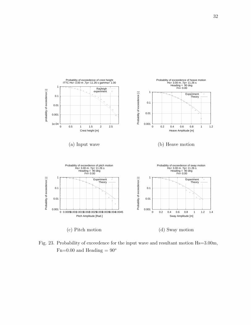
23 Probability of exceedence for the input wave and resultant motion
Hs=3.00m, Fn=0.00 and Heading = 90o . . . . . . . . . . . . . . . . 32
24 Probability of exceedence for the input wave and resultant motion
Hs=3.00m, Fn=0.00 and Heading = 90o . . . . . . . . . . . . . . . . 33
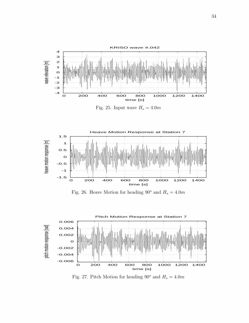
25 Input wave Hs = 4.0m . . . . . . . . . . . . . . . . . . . . . . . . . . 34
26 Heave Motion for heading 90o and Hs = 4.0m . . . . . . . . . . . . . 34
27 Pitch Motion for heading 90o and Hs = 4.0m . . . . . . . . . . . . . 34
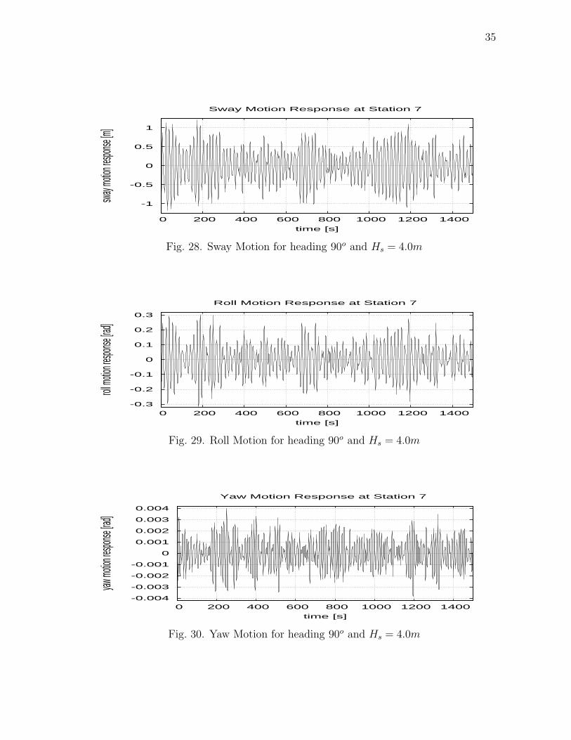
28 Sway Motion for heading 90o and Hs = 4.0m . . . . . . . . . . . . . 35
29 Roll Motion for heading 90o and Hs = 4.0m . . . . . . . . . . . . . . 35
30 Yaw Motion for heading 90o and Hs = 4.0m . . . . . . . . . . . . . . 35
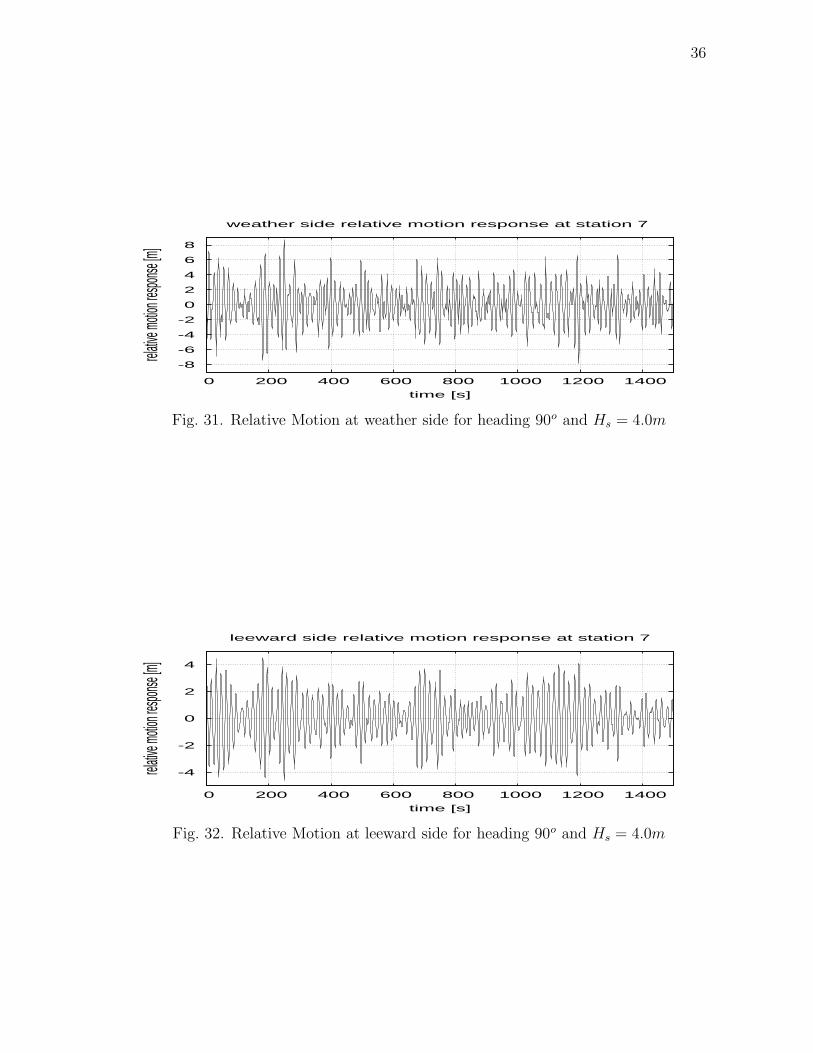
31 Relative Motion at weather side for heading 90o and Hs = 4.0m . . . 36
32 Relative Motion at leeward side for heading 90o and Hs = 4.0m . . . 36
33 Probability of exceedence for the input wave and resultant motion
Hs=4.00m, Fn=0.00 and Heading = 90o . . . . . . . . . . . . . . . . 37
34 Probability of exceedence for the input wave and resultant motion
Hs=4.00m, Fn=0.00 and Heading = 90o . . . . . . . . . . . . . . . . 38
35 Input wave Hs = 6.0m . . . . . . . . . . . . . . . . . . . . . . . . . . 39
36 Heave Motion for heading 90o and Hs = 6.0m . . . . . . . . . . . . . 39
37 Pitch Motion for heading 90o and Hs = 6.0m . . . . . . . . . . . . . 40
38 Sway Motion for heading 90o and Hs = 6.0m . . . . . . . . . . . . . 40
xii
FIGURE Page
39 Roll Motion for heading 90o and Hs = 6.0m . . . . . . . . . . . . . . 40
40 Yaw Motion for heading 90o and Hs = 6.0m . . . . . . . . . . . . . . 41
41 Relative Motion at weather side for heading 90o and Hs = 6.0m . . . 41
42 Relative Motion at leeward side for heading 90o and Hs = 6.0m . . . 41
43 Probability of exceedence for the input wave and resultant motion
Hs=6.00m, Fn=0.00 and Heading = 90o . . . . . . . . . . . . . . . . 42
44 Probability of exceedence for the input wave and resultant motion
Hs=6.00m, Fn=0.00 and Heading = 90o . . . . . . . . . . . . . . . . 43
45 Input wave Hs = 7.0m . . . . . . . . . . . . . . . . . . . . . . . . . . 44
46 Heave Motion for heading 90o and Hs = 7.0m . . . . . . . . . . . . . 44
47 Pitch Motion for heading 90o and Hs = 7.0m . . . . . . . . . . . . . 45
48 Sway Motion for heading 90o and Hs = 7.0m . . . . . . . . . . . . . 45
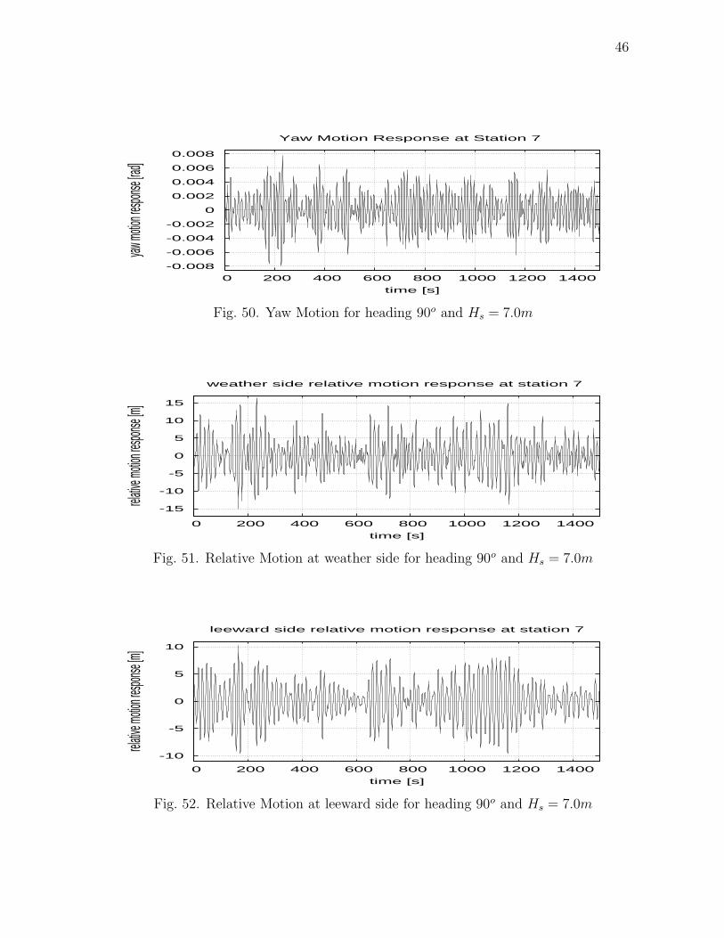
49 Roll Motion for heading 90o and Hs = 7.0m . . . . . . . . . . . . . . 45
50 Yaw Motion for heading 90o and Hs = 7.0m . . . . . . . . . . . . . . 46
51 Relative Motion at weather side for heading 90o and Hs = 7.0m . . . 46
52 Relative Motion at leeward side for heading 90o and Hs = 7.0m . . . 46
53 Probability of exceedence for the input wave and resultant motion
Hs=7.00m, Fn=0.00 and Heading = 90o . . . . . . . . . . . . . . . . 47
54 Probability of exceedence for the input wave and resultant motion
Hs=7.00m, Fn=0.00 and Heading = 90o . . . . . . . . . . . . . . . . 48
55 Input wave Hs = 9.0m . . . . . . . . . . . . . . . . . . . . . . . . . . 49
56 Heave Motion for heading 90o and Hs = 9.0m . . . . . . . . . . . . . 49
57 Pitch Motion for heading 90o and Hs = 9.0m . . . . . . . . . . . . . 50
58 Sway Motion for heading 90o and Hs = 9.0m . . . . . . . . . . . . . 50
xiii
FIGURE Page
59 Roll Motion for heading 90o and Hs = 9.0m . . . . . . . . . . . . . . 50
60 Yaw Motion for heading 90o and Hs = 9.0m . . . . . . . . . . . . . . 51
61 Relative Motion at weather side for heading 90o and Hs = 9.0m . . . 51
62 Relative Motion at leeward side for heading 90o and Hs = 9.0m . . . 51
63 Probability of exceedence for the input wave and resultant motion
Hs=9.00m, Fn=0.00 and Heading = 90o . . . . . . . . . . . . . . . . 52
64 Probability of exceedence for the input wave and resultant motion
Hs=9.00m, Fn=0.00 and Heading = 90o . . . . . . . . . . . . . . . . 53
65 Input wave Hs = 11.0m . . . . . . . . . . . . . . . . . . . . . . . . . 54
66 Heave Motion for heading 90o and Hs = 11.0m . . . . . . . . . . . . 54
67 Pitch Motion for heading 90o and Hs = 11.0m . . . . . . . . . . . . . 55
68 Sway Motion for heading 90o and Hs = 11.0m . . . . . . . . . . . . . 55
69 Roll Motion for heading 90o and Hs = 11.0m . . . . . . . . . . . . . 55
70 Yaw Motion for heading 90o and Hs = 11.0m . . . . . . . . . . . . . 56
71 Relative Motion at weather side for heading 90o and Hs = 9.0m . . . 56
72 Relative Motion at leeward side for heading 90o and Hs = 9.0m . . . 56
73 Probability of exceedence for the input wave and resultant motion
Hs=11.00m, Fn=0.00 and Heading = 90o . . . . . . . . . . . . . . . 57
74 Probability of exceedence for the input wave and resultant motion
Hs=11.00m, Fn=0.00 and Heading = 90o . . . . . . . . . . . . . . . 58
75 Peak value comparison for heave, pitch,sway,roll and vertical rel-
ative motions (weather side and leeward side) for Fn=0.00 and
Heading = 90o . . . . . . . . . . . . . . . . . . . . . . . . . . . . . . 59
76 Peak value comparison for yaw motion, Fn=0.00 and Heading = 90o 60

xiv
FIGURE Page
77 Input wave Hs = 3.0m . . . . . . . . . . . . . . . . . . . . . . . . . . 62
78 Heave Motion for heading 135o and Hs = 3.0m . . . . . . . . . . . . 62
79 Pitch Motion for heading 135o and Hs = 3.0m . . . . . . . . . . . . . 62
80 Sway Motion for heading 135o and Hs = 3.0m . . . . . . . . . . . . . 63
81 Roll Motion for heading 135o and Hs = 3.0m . . . . . . . . . . . . . 63
82 Yaw Motion for heading 135o and Hs = 3.0m . . . . . . . . . . . . . 63
83 Relative Motion at weather side for heading 135o and Hs = 3.0m . . 64
84 Relative Motion at leeward side for heading 135o and Hs = 3.0m . . 64
85 Probability of exceedence for the input wave and resultant motion
Hs=3.00m, Fn=0.15 and Heading = 135o . . . . . . . . . . . . . . . 65
86 Probability of exceedence for the input wave and resultant motion
Hs=3.00m, Fn=0.15 and Heading = 135o . . . . . . . . . . . . . . . 66
87 Input wave Hs = 4.0m . . . . . . . . . . . . . . . . . . . . . . . . . . 67
88 Heave Motion for heading 135o and Hs = 4.0m . . . . . . . . . . . . 67
89 Pitch Motion for heading 135o and Hs = 4.0m . . . . . . . . . . . . . 67
90 Sway Motion for heading 135o and Hs = 4.0m . . . . . . . . . . . . . 68
91 Roll Motion for heading 135o and Hs = 4.0m . . . . . . . . . . . . . 68
92 Yaw Motion for heading 135o and Hs = 4.0m . . . . . . . . . . . . . 68
93 Relative Motion at weather side for heading 135o and Hs = 4.0m . . 69
94 Relative Motion at leeward side for heading 135o and Hs = 4.0m . . 69
95 Probability of exceedence for the input wave and resultant motion
Hs=4.00m, Fn=0.15 and Heading = 135o . . . . . . . . . . . . . . . 70
96 Probability of exceedence for the input wave and resultant motion
Hs=4.00m, Fn=0.15 and Heading = 135o . . . . . . . . . . . . . . . 71

xv
FIGURE Page
97 Input wave Hs = 6.0m . . . . . . . . . . . . . . . . . . . . . . . . . . 72
98 Heave Motion for heading 135o and Hs = 6.0m . . . . . . . . . . . . 72
99 Pitch Motion for heading 135o and Hs = 6.0m . . . . . . . . . . . . . 73
100 Sway Motion for heading 135o and Hs = 6.0m . . . . . . . . . . . . . 73
101 Roll Motion for heading 135o and Hs = 6.0m . . . . . . . . . . . . . 73
102 Yaw Motion for heading 135o and Hs = 6.0m . . . . . . . . . . . . . 74
103 Relative Motion at weather side for heading 135o and Hs = 6.0m . . 74
104 Relative Motion at leeward side for heading 135o and Hs = 6.0m . . 74
105 Probability of exceedence for the input wave and resultant motion
Hs=6.00m, Fn=0.15 and Heading = 135o . . . . . . . . . . . . . . . 75
106 Probability of exceedence for the input wave and resultant motion
Hs=6.00m, Fn=0.15 and Heading = 135o . . . . . . . . . . . . . . . 76
107 Input wave Hs = 7.0m . . . . . . . . . . . . . . . . . . . . . . . . . . 77
108 Heave Motion for heading 135o and Hs = 7.0m . . . . . . . . . . . . 77
109 Pitch Motion for heading 135o and Hs = 7.0m . . . . . . . . . . . . . 78
110 Sway Motion for heading 135o and Hs = 7.0m . . . . . . . . . . . . . 78
111 Roll Motion for heading 135o and Hs = 7.0m . . . . . . . . . . . . . 78
112 Yaw Motion for heading 135o and Hs = 7.0m . . . . . . . . . . . . . 79
113 Relative Motion at weather side for heading 135o and Hs = 7.0m . . 79
114 Relative Motion at leeward side for heading 135o and Hs = 7.0m . . 79
115 Probability of exceedence for the input wave and resultant motion
Hs=7.00m, Fn=0.15 and Heading = 135o . . . . . . . . . . . . . . . 80
116 Probability of exceedence for the input wave and resultant motion
Hs=7.00m, Fn=0.15 and Heading = 135o . . . . . . . . . . . . . . . 81
xvi
FIGURE Page
117 Input wave Hs = 9.0m . . . . . . . . . . . . . . . . . . . . . . . . . . 82
118 Heave Motion for heading 135o and Hs = 9.0m . . . . . . . . . . . . 82
119 Pitch Motion for heading 135o and Hs = 9.0m . . . . . . . . . . . . . 83
120 Sway Motion for heading 135o and Hs = 9.0m . . . . . . . . . . . . . 83
121 Roll Motion for heading 135o and Hs = 9.0m . . . . . . . . . . . . . 83
122 Yaw Motion for heading 135o and Hs = 9.0m . . . . . . . . . . . . . 84
123 Relative Motion at weather side for heading 135o and Hs = 9.0m . . 84
124 Relative Motion at leeward side for heading 135o and Hs = 9.0m . . 84
125 Probability of exceedence for the input wave and resultant motion
Hs=9.00m, Fn=0.15 and Heading = 135o . . . . . . . . . . . . . . . 85
126 Probability of exceedence for the input wave and resultant motion
Hs=9.00m, Fn=0.15 and Heading = 135o . . . . . . . . . . . . . . . 86
127 Input wave Hs = 11.0m . . . . . . . . . . . . . . . . . . . . . . . . . 87
128 Heave Motion for heading 135o and Hs = 11.0m . . . . . . . . . . . . 87
129 Pitch Motion for heading 135o and Hs = 11.0m . . . . . . . . . . . . 88
130 Sway Motion for heading 135o and Hs = 11.0m . . . . . . . . . . . . 88
131 Roll Motion for heading 135o and Hs = 11.0m . . . . . . . . . . . . . 88
132 Yaw Motion for heading 135o and Hs = 11.0m . . . . . . . . . . . . . 89
133 Relative Motion at weather side for heading 135o and Hs = 9.0m . . 89
134 Relative Motion at leeward side for heading 135o and Hs = 9.0m . . 89
135 Probability of exceedence for the input wave and resultant motion
Hs=11.00m, Fn=0.15 and Heading = 135o . . . . . . . . . . . . . . . 90
136 Probability of exceedence for the input wave and resultant motion
Hs=11.00m, Fn=0.15 and Heading = 135o . . . . . . . . . . . . . . . 91
xvii
FIGURE Page
137 Peak value comparison for heave, pitch,sway,roll and vertical rel-
ative motions (weather side and leeward side) for Fn=0.15 and
Heading = 135o . . . . . . . . . . . . . . . . . . . . . . . . . . . . . . 92
138 Peak value comparison for yaw motion, Fn=0.15 and Heading = 135o 93
139 Input wave Hs = 3.0m . . . . . . . . . . . . . . . . . . . . . . . . . . 95
140 Heave Motion for heading 180o and Hs = 3.0m . . . . . . . . . . . . 95
141 Pitch Motion for heading 180o and Hs = 3.0m . . . . . . . . . . . . . 95
142 Relative Motion at weather side for heading 180o and Hs = 3.0m . . 96
143 Relative Motion at leeward side for heading 180o and Hs = 3.0m . . 96
144 Probability of exceedence for the input wave and resultant motion
Hs=3.00m, Fn=0 and Heading = 180o . . . . . . . . . . . . . . . . . 97
145 Probability of exceedence for vertical relative motion (leeward
side) Hs=3.00m, Fn=0 and Heading = 180o . . . . . . . . . . . . . . 98
146 Input wave Hs = 4.0m . . . . . . . . . . . . . . . . . . . . . . . . . . 98
147 Heave Motion for heading 180o and Hs = 4.0m . . . . . . . . . . . . 98
148 Pitch Motion for heading 180o and Hs = 4.0m . . . . . . . . . . . . . 99
149 Relative Motion at weather side for heading 180o and Hs = 4.0m . . 99
150 Relative Motion at leeward side for heading 180o and Hs = 4.0m . . 99
151 Probability of exceedence for the input wave and resultant motion
Hs=4.00m, Fn=0 and Heading = 180o . . . . . . . . . . . . . . . . . 100
152 Probability of exceedence for vertical relative motion (leeward
side) Hs=4.00m, Fn=0 and Heading = 180o . . . . . . . . . . . . . . 101
153 Input wave Hs = 6.0m . . . . . . . . . . . . . . . . . . . . . . . . . . 101
154 Heave Motion for heading 180o and Hs = 6.0m . . . . . . . . . . . . 102
xviii
FIGURE Page
155 Pitch Motion for heading 180o and Hs = 6.0m . . . . . . . . . . . . . 102
156 Relative Motion at weather side for heading 180o and Hs = 6.0m . . 102
157 Relative Motion at leeward side for heading 180o and Hs = 6.0m . . 103
158 Probability of exceedence for the input wave and resultant motion
Hs=6.00m, Fn=0 and Heading = 180o . . . . . . . . . . . . . . . . . 104
159 Probability of exceedence for the vertical relative motion (leeward
side) Hs=6.00m, Fn=0 and Heading = 180o . . . . . . . . . . . . . . 105
160 Input wave Hs = 7.0m . . . . . . . . . . . . . . . . . . . . . . . . . . 106
161 Heave Motion for heading 180o and Hs = 7.0m . . . . . . . . . . . . 106
162 Pitch Motion for heading 180o and Hs = 7.0m . . . . . . . . . . . . . 107
163 Relative Motion at weather side for heading 180o and Hs = 7.0m . . 107
164 Relative Motion at leeward side for heading 180o and Hs = 7.0m . . 107
165 Probability of exceedence for the input wave and resultant motion
Hs=7.00m, Fn=0 and Heading = 180o . . . . . . . . . . . . . . . . . 108
166 Probability of exceedence for vertical relative motion (leeward
side) Hs=7.00m, Fn=0 and Heading = 180o . . . . . . . . . . . . . . 109
167 Input wave Hs = 9.0m . . . . . . . . . . . . . . . . . . . . . . . . . . 110
168 Heave Motion for heading 180o and Hs = 9.0m . . . . . . . . . . . . 110
169 Pitch Motion for heading 180o and Hs = 9.0m . . . . . . . . . . . . . 111
170 Relative Motion at weather side for heading 180o and Hs = 9.0m . . 111
171 Relative Motion at leeward side for heading 180o and Hs = 9.0m . . 111
172 Probability of exceedence for the input wave and resultant motion
Hs=9.00m, Fn=0 and Heading = 180o . . . . . . . . . . . . . . . . . 112
xix
FIGURE Page
173 Probability of exceedence for vertical relative motion (leeward
side) Hs=9.00m, Fn=0 and Heading = 180o . . . . . . . . . . . . . . 113
174 Input wave Hs = 9.0m . . . . . . . . . . . . . . . . . . . . . . . . . . 114
175 Heave Motion for heading 180o and Hs = 11.0m . . . . . . . . . . . . 114
176 Pitch Motion for heading 180o and Hs = 11.0m . . . . . . . . . . . . 115
177 Relative Motion at weather side for heading 180o and Hs = 9.0m . . 115
178 Relative Motion at leeward side for heading 180o and Hs = 9.0m . . 115
179 Probability of exceedence for the input wave and resultant motion
Hs=11.00m, Fn=0 and Heading = 180o . . . . . . . . . . . . . . . . 116
180 Probability of exceedence for the vertical relative motion (leeward
side) Hs=11.00m, Fn=0 and Heading = 180o . . . . . . . . . . . . . 117
181 Peak value comparison for heave, pitch,sway,roll and vertical rela-
tive motions (weather side and leeward side) for Fn=0 and Head-
ing = 180o . . . . . . . . . . . . . . . . . . . . . . . . . . . . . . . . . 118
182 Peak value comparison for heave, pitch,sway,roll and vertical rel-
ative motions (weather side and leeward side) for Fn=0.00 and
Heading = 135o . . . . . . . . . . . . . . . . . . . . . . . . . . . . . . 120
183 Peak value comparison for yaw motion, Fn=0.00 and Heading = 135o 121
184 Peak value comparison for heave, pitch, sway, roll, and vertical
relative motions (weather side and leeward side) for Fn=0 and
Heading = 180o . . . . . . . . . . . . . . . . . . . . . . . . . . . . . . 121
1
CHAPTER I
INTRODUCTION
1. Motivation
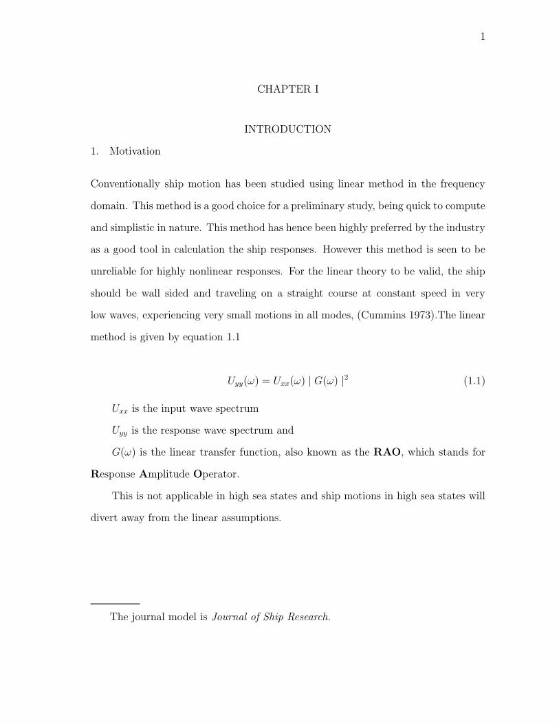
Conventionally ship motion has been studied using linear method in the frequency
domain. This method is a good choice for a preliminary study, being quick to compute
and simplistic in nature. This method has hence been highly preferred by the industry
as a good tool in calculation the ship responses. However this method is seen to be
unreliable for highly nonlinear responses. For the linear theory to be valid, the ship
should be wall sided and traveling on a straight course at constant speed in very
low waves, experiencing very small motions in all modes, (Cummins 1973).The linear
method is given by equation 1.1
Uyy(ω) = Uxx(ω) | G(ω) |2 (1.1)
Uxx is the input wave spectrum
Uyy is the response wave spectrum and
G(ω) is the linear transfer function, also known as the RAO, which stands for
Response Amplitude Operator.
This is not applicable in high sea states and ship motions in high sea states will
divert away from the linear assumptions.
The journal model is Journal of Ship Research.
2
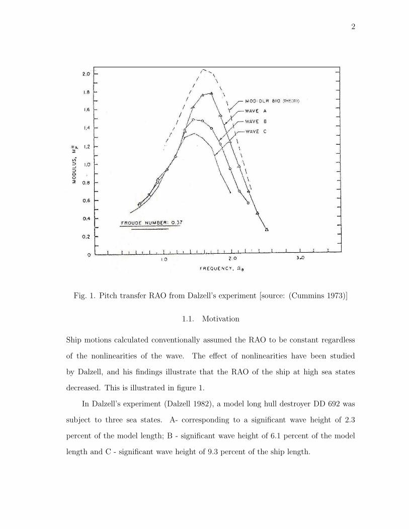
Fig. 1. Pitch transfer RAO from Dalzell’s experiment [source: (Cummins 1973)]
1.1. Motivation
Ship motions calculated conventionally assumed the RAO to be constant regardless
of the nonlinearities of the wave. The effect of nonlinearities have been studied
by Dalzell, and his findings illustrate that the RAO of the ship at high sea states
decreased. This is illustrated in figure 1.
In Dalzell’s experiment (Dalzell 1982), a model long hull destroyer DD 692 was
subject to three sea states. A- corresponding to a significant wave height of 2.3
percent of the model length; B - significant wave height of 6.1 percent of the model
length and C - significant wave height of 9.3 percent of the ship length.
3
For these sea conditions, the hull was towed to find the pitch responses, from
which RAOs were generated as shown in equation 1.2.
RAO =Uxy
Uxx(1.2)
where the subscript x and y denote the input wave and the response respectively.
The objective of the study is to compare the motions predicted by the linear
method in the frequency domain and simulation in the time domain. Analysis will be
performed for different Froude numbers and headings. Such a study would confirm
the application of UNIOM on more effective calculations of ship motion.
The additional margin that we may get using this method would help set lower
margin to prevent the shipping of green water, which is dealt by classification so-
cieties by defining a minimum freeboard requirement. The International Load Line
Convention (ILLC) 1996 has specified minimum freeboard requirements for the ship.
The UNIOM model presented in this work will help us better understand the role of
wave nonlinearities on the ship motions and thereby the margin of safety required.
1.2. Application
We apply a Universal Nonlinear Input Output Model , henceforth called UNIOM.
The method uses the linear RAO of the ship, and uses the nonlinear input wave
to simulate a non-linear response model. This method uses the real wave, instead
of a Gaussian wave package simulated using the sea spectrum. This approach has
previously been used by Adil (Adil 2004) and Richer (Richer 2005). A detailed
description of this method is given by Kim, C. H. (Kim 2006).
We do not have sufficient experimental data to confidently say that one method
is superior to the other, however we can see how the responses from the linear and
4
the UNIOM approach differ as the sea state increases.
2. Approach
2.1. Linear and Nonlinear Model
For a Gaussian input wave pattern input into a linear system, the response is give
by equation 1.1. A linear system thus can be analyzed using this approach. This
approach is called the linear approach.
The non linear input into a linear system would produce a non linear response.
This non linear response can be studied in the time domain using the relation
Out(t) = Σ | Aj || RAOj | ei(ωj t−φj−εj) (1.3)
The subscript j denotes the jth frequency.
Out(t) is the output time series, which depends on the RAO, RAOj, if the RAO
is the roll motion RAO then Out(t) gives the time series of roll motion. Similarly on
using the relative motion RAO in the formula, Out(t) becomes the relative motion
time series. Thus we can simulate any motion provided we know the RAO.
The RAO is generated from strip theory, and εj is the phase of the RAO. Since
the input Aj is nonlinear, Out(t), the resultant response of the vessel, even though
the RAO is linear, is also nonlinear.
The above approach is called the UNIOM model.
5
CHAPTER II
THE UNIOM MODEL
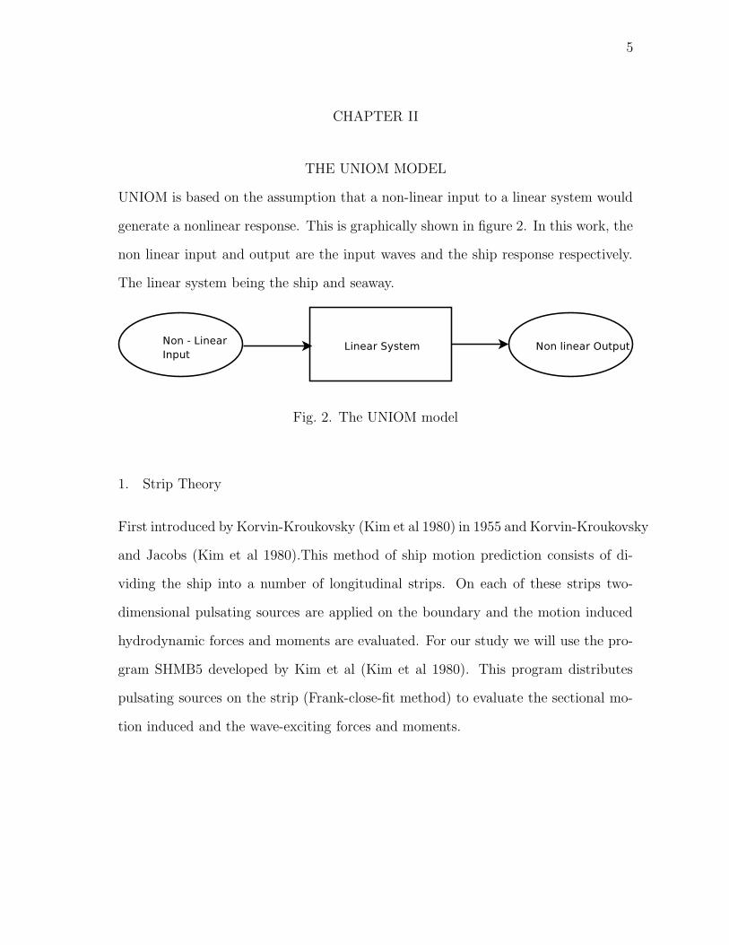
UNIOM is based on the assumption that a non-linear input to a linear system would
generate a nonlinear response. This is graphically shown in figure 2. In this work, the
non linear input and output are the input waves and the ship response respectively.
The linear system being the ship and seaway.
Fig. 2. The UNIOM model
1. Strip Theory
First introduced by Korvin-Kroukovsky (Kim et al 1980) in 1955 and Korvin-Kroukovsky
and Jacobs (Kim et al 1980).This method of ship motion prediction consists of di-
viding the ship into a number of longitudinal strips. On each of these strips two-
dimensional pulsating sources are applied on the boundary and the motion induced
hydrodynamic forces and moments are evaluated. For our study we will use the pro-
gram SHMB5 developed by Kim et al (Kim et al 1980). This program distributes
pulsating sources on the strip (Frank-close-fit method) to evaluate the sectional mo-
tion induced and the wave-exciting forces and moments.
6
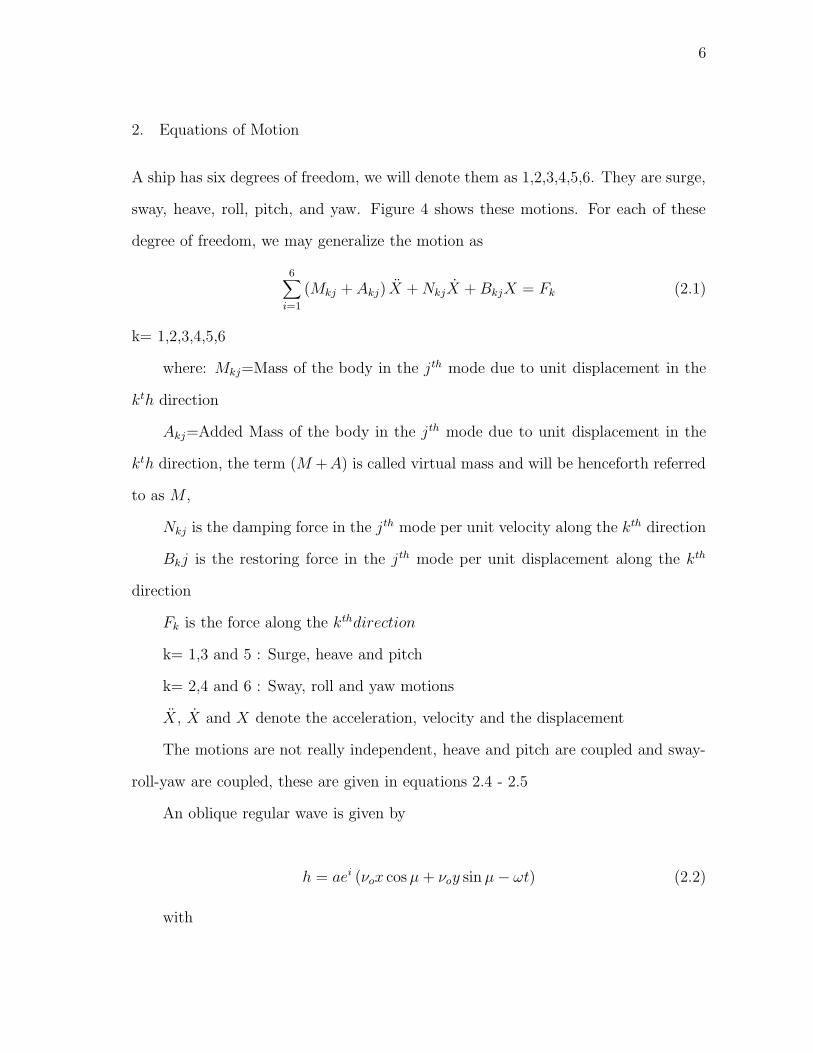
2. Equations of Motion
A ship has six degrees of freedom, we will denote them as 1,2,3,4,5,6. They are surge,
sway, heave, roll, pitch, and yaw. Figure 4 shows these motions. For each of these
degree of freedom, we may generalize the motion as
6∑
i=1
(Mkj + Akj) X +NkjX +BkjX = Fk (2.1)
k= 1,2,3,4,5,6
where: Mkj=Mass of the body in the jth mode due to unit displacement in the
kth direction
Akj=Added Mass of the body in the jth mode due to unit displacement in the
kth direction, the term (M +A) is called virtual mass and will be henceforth referred
to as M ,
Nkj is the damping force in the jth mode per unit velocity along the kth direction
Bkj is the restoring force in the jth mode per unit displacement along the kth
direction
Fk is the force along the kthdirection
k= 1,3 and 5 : Surge, heave and pitch
k= 2,4 and 6 : Sway, roll and yaw motions
X, X and X denote the acceleration, velocity and the displacement
The motions are not really independent, heave and pitch are coupled and sway-
roll-yaw are coupled, these are given in equations 2.4 - 2.5
An oblique regular wave is given by
h = aei (νox cosµ+ νoy sin µ− ωt) (2.2)
with
7
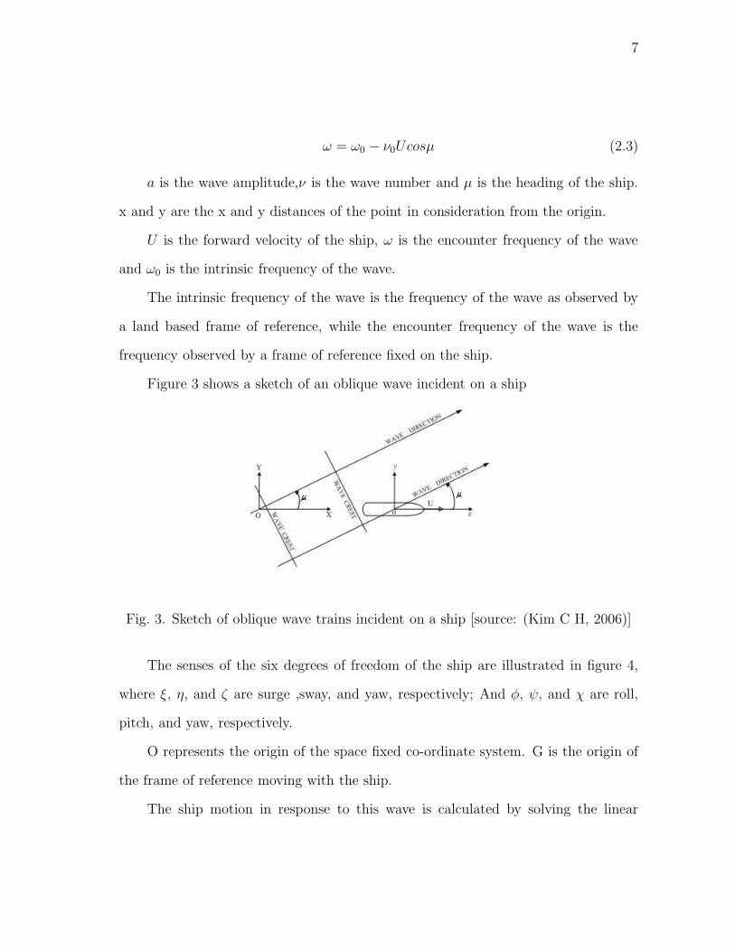
ω = ω0 − ν0Ucosµ (2.3)
a is the wave amplitude,ν is the wave number and µ is the heading of the ship.
x and y are the x and y distances of the point in consideration from the origin.
U is the forward velocity of the ship, ω is the encounter frequency of the wave
and ω0 is the intrinsic frequency of the wave.
The intrinsic frequency of the wave is the frequency of the wave as observed by
a land based frame of reference, while the encounter frequency of the wave is the
frequency observed by a frame of reference fixed on the ship.
Figure 3 shows a sketch of an oblique wave incident on a ship
Fig. 3. Sketch of oblique wave trains incident on a ship [source: (Kim C H, 2006)]
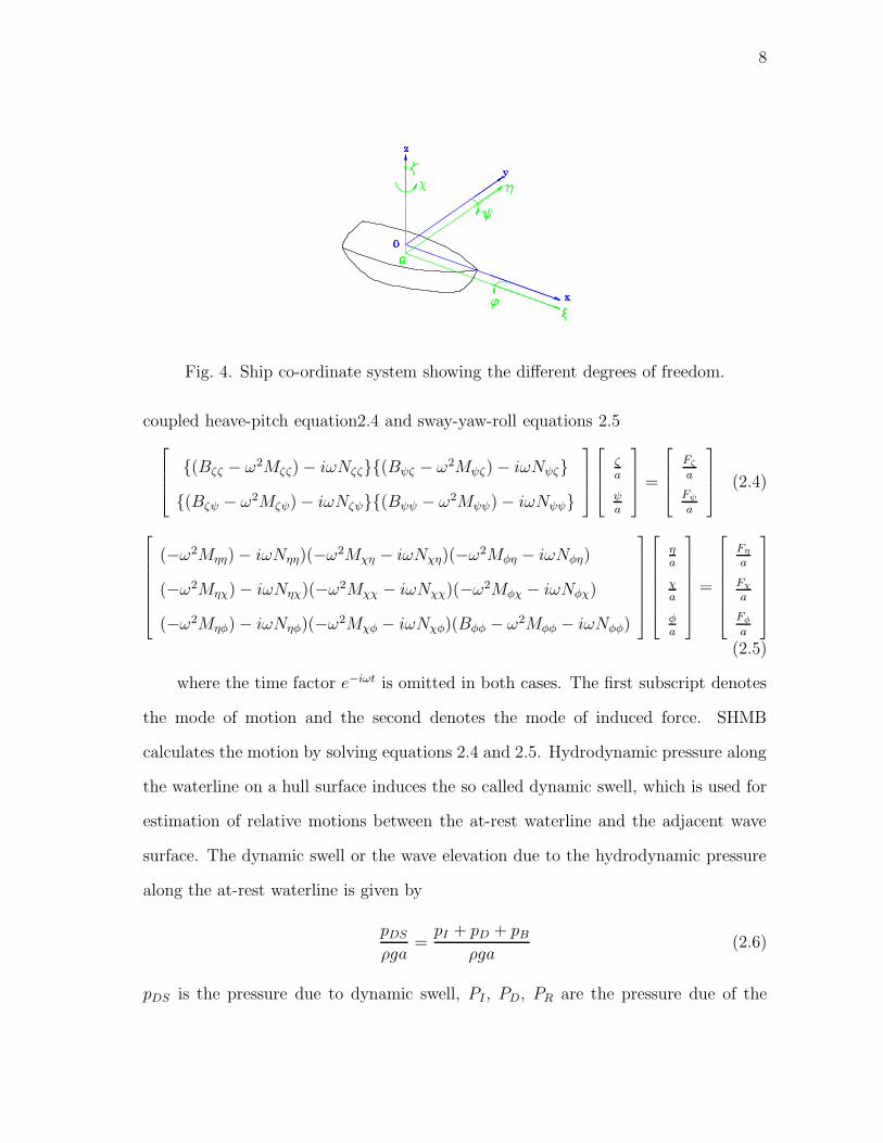
The senses of the six degrees of freedom of the ship are illustrated in figure 4,
where ξ, η, and ζ are surge ,sway, and yaw, respectively; And φ, ψ, and χ are roll,
pitch, and yaw, respectively.
O represents the origin of the space fixed co-ordinate system. G is the origin of
the frame of reference moving with the ship.
The ship motion in response to this wave is calculated by solving the linear
8
Fig. 4. Ship co-ordinate system showing the different degrees of freedom.
coupled heave-pitch equation2.4 and sway-yaw-roll equations 2.5
{(Bζζ − ω2Mζζ) − iωNζζ}{(Bψζ − ω2Mψζ) − iωNψζ}
{(Bζψ − ω2Mζψ) − iωNζψ}{(Bψψ − ω2Mψψ) − iωNψψ}
ζ
a
ψ
a
=
Fζa
Fψa
(2.4)
(−ω2Mηη) − iωNηη)(−ω2Mχη − iωNχη)(−ω2Mφη − iωNφη)
(−ω2Mηχ) − iωNηχ)(−ω2Mχχ − iωNχχ)(−ω2Mφχ − iωNφχ)
(−ω2Mηφ) − iωNηφ)(−ω2Mχφ − iωNχφ)(Bφφ − ω2Mφφ − iωNφφ)
η
a
χ
a
φ
a
=
Fηa
Fχa
Fφa
(2.5)
where the time factor e−iωt is omitted in both cases. The first subscript denotes
the mode of motion and the second denotes the mode of induced force. SHMB
calculates the motion by solving equations 2.4 and 2.5. Hydrodynamic pressure along
the waterline on a hull surface induces the so called dynamic swell, which is used for
estimation of relative motions between the at-rest waterline and the adjacent wave
surface. The dynamic swell or the wave elevation due to the hydrodynamic pressure
along the at-rest waterline is given by
pDS
ρga=pI + pD + pB
ρga(2.6)
pDS is the pressure due to dynamic swell, PI , PD, PR are the pressure due of the
9
incident, diffraction and the radiation wave. the vertical motion z± of the at-rest
waterline itself is given by
z± = ζ − xψ +iU
ωψ ∓ B(x)
2φ (2.7)
where ± indicates the right and left sides of the ship section along the waterline
respectively. B(x)2
indicates the half section beam in the waterplane. Therefore the
relative motion between the at rest waterline and the wave surface, the dynamic swell
is given by
r±a
=pDS±ρga
− z±a
(2.8)
3. The Ship Motion Program
The ship motion is analyzed using SHMB5, developed by Kim, C.H. et al. This
program uses strip theory for computations, the use of this software has been validated
and the method is specified in Kim, C.H et al (Kim et al 1980). The output from the
program is further processed by the program PRDMR5, to give the relative motion.
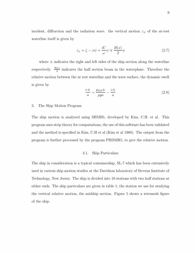
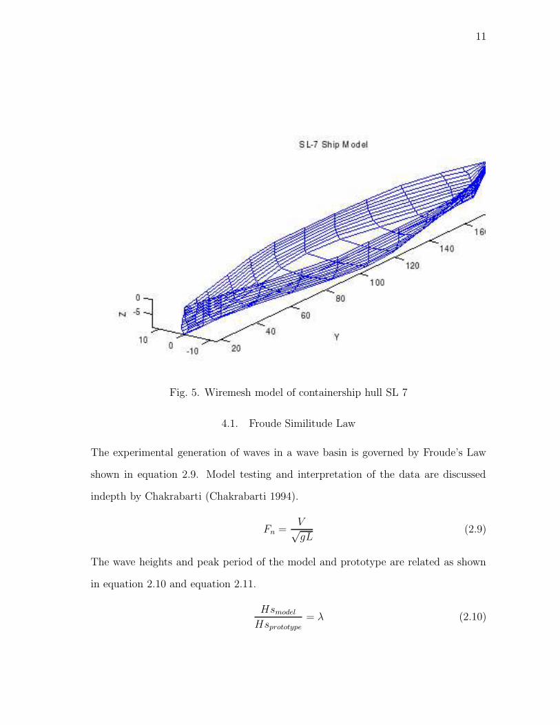
3.1. Ship Particulars
The ship in consideration is a typical containership, SL-7 which has been extensively
used in various ship motion studies at the Davidson laboratory of Stevens Institute of
Technology, New Jersey. The ship is divided into 10 stations with two half stations at
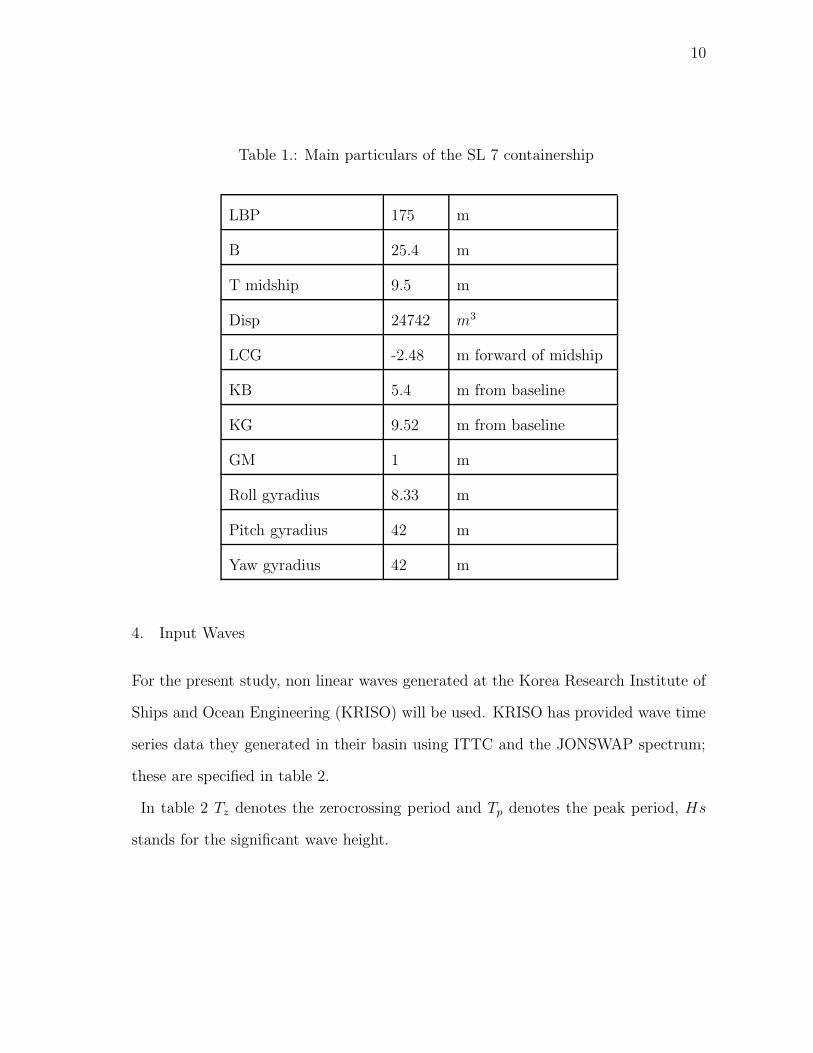
either ends. The ship particulars are given in table 1, the station we use for studying
the vertical relative motion, the midship section. Figure 5 shows a wiremesh figure
of the ship.
10
Table 1.: Main particulars of the SL 7 containership
LBP 175 m
B 25.4 m
T midship 9.5 m
Disp 24742 m3
LCG -2.48 m forward of midship
KB 5.4 m from baseline
KG 9.52 m from baseline
GM 1 m
Roll gyradius 8.33 m
Pitch gyradius 42 m
Yaw gyradius 42 m
4. Input Waves
For the present study, non linear waves generated at the Korea Research Institute of
Ships and Ocean Engineering (KRISO) will be used. KRISO has provided wave time
series data they generated in their basin using ITTC and the JONSWAP spectrum;
these are specified in table 2.
In table 2 Tz denotes the zerocrossing period and Tp denotes the peak period, Hs
stands for the significant wave height.
11
Fig. 5. Wiremesh model of containership hull SL 7
4.1. Froude Similitude Law
The experimental generation of waves in a wave basin is governed by Froude’s Law
shown in equation 2.9. Model testing and interpretation of the data are discussed
indepth by Chakrabarti (Chakrabarti 1994).
Fn =V√gL
(2.9)
The wave heights and peak period of the model and prototype are related as shown
in equation 2.10 and equation 2.11.
Hsmodel
Hsprototype= λ (2.10)
12
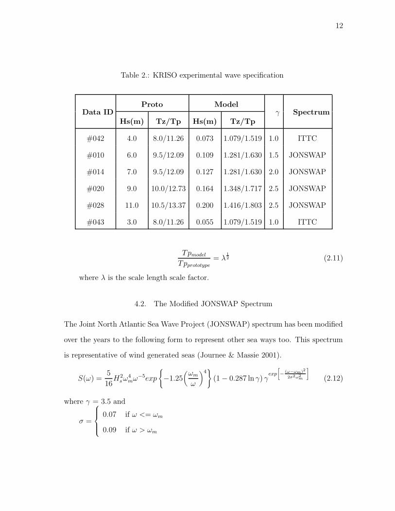
Table 2.: KRISO experimental wave specification
Data IDProto Model
γ SpectrumHs(m) Tz/Tp Hs(m) Tz/Tp
#042 4.0 8.0/11.26 0.073 1.079/1.519 1.0 ITTC
#010 6.0 9.5/12.09 0.109 1.281/1.630 1.5 JONSWAP
#014 7.0 9.5/12.09 0.127 1.281/1.630 2.0 JONSWAP
#020 9.0 10.0/12.73 0.164 1.348/1.717 2.5 JONSWAP
#028 11.0 10.5/13.37 0.200 1.416/1.803 2.5 JONSWAP
#043 3.0 8.0/11.26 0.055 1.079/1.519 1.0 ITTC
Tpmodel
Tpprototype= λ
12 (2.11)
where λ is the scale length scale factor.
4.2. The Modified JONSWAP Spectrum
The Joint North Atlantic Sea Wave Project (JONSWAP) spectrum has been modified
over the years to the following form to represent other sea ways too. This spectrum
is representative of wind generated seas (Journee & Massie 2001).
S(ω) =5
16H2sω
4mω
−5exp
{
−1.25(
ωm
ω
)4}
(1 − 0.287 ln γ) γexp
[
−(ω−ωm)2
2σ2ω2m
]
(2.12)
where γ = 3.5 and
σ =
0.07 if ω <= ωm
0.09 if ω > ωm
13
4.3. ITTC Spectrum
The 15th International Towing Tank Conference (ITTC 1978) has proposed a theo-
retical spectrum for average sea conditions and not for fully developed seas, given the
significant wave height and modal period.
S(ω) =A
ω2exp
(
B
ω4
)
, A = 173H2sT
−41 , B = 691 (T1)
2 (2.13)
The above spectra are discussed by Dean, Robert G. and Dalrymple, Robert A. (Dean
& Dalrymple 1984)
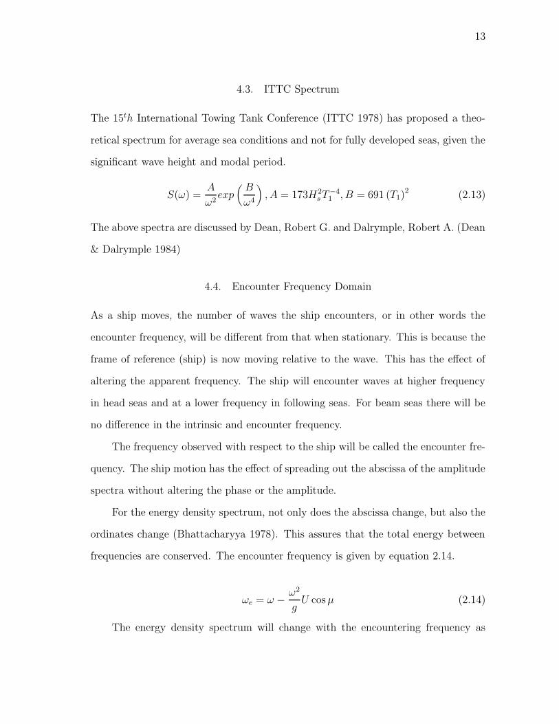
4.4. Encounter Frequency Domain
As a ship moves, the number of waves the ship encounters, or in other words the
encounter frequency, will be different from that when stationary. This is because the
frame of reference (ship) is now moving relative to the wave. This has the effect of
altering the apparent frequency. The ship will encounter waves at higher frequency
in head seas and at a lower frequency in following seas. For beam seas there will be
no difference in the intrinsic and encounter frequency.
The frequency observed with respect to the ship will be called the encounter fre-
quency. The ship motion has the effect of spreading out the abscissa of the amplitude
spectra without altering the phase or the amplitude.
For the energy density spectrum, not only does the abscissa change, but also the
ordinates change (Bhattacharyya 1978). This assures that the total energy between
frequencies are conserved. The encounter frequency is given by equation 2.14.
ωe = ω − ω2
gU cosµ (2.14)
The energy density spectrum will change with the encountering frequency as

14
below
Uxx (ωe) = Uxx (ω)
(
1 − 2ωU
gcosµ
)−1
(2.15)
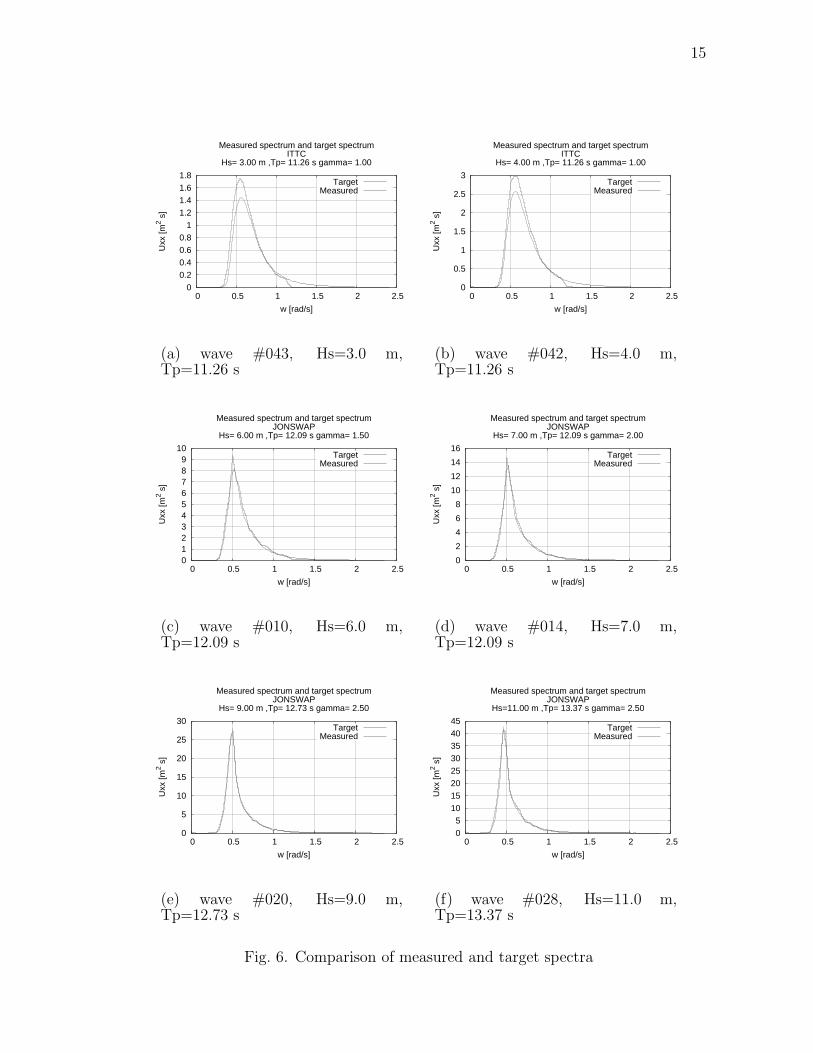
5. KRISO Data Analysis
Prototype waves from KRISO are processed through a Fast Fourier Transform (FFT)
program to obtain the energy density spectrum. The energy density spectrum is
smoothed to obtain a smooth curve. Accuracy of the KRISO generated waves are
assured by comparing the measured spectrum to the target spectrum, a 10% error
in variance is considered allowable. Table 3 shows the comparison of variance of the
measured and target spectrum.
To facilitate visual inspection, graphs are plotted comparing the measured and
target spectra for each sea state. Overall good agreement is seen between the mea-
sured and the target spectra. Figures 6(a) to 6(f) compares the measured and target
spectra.
6. Response Analysis
We can now simulate the motion of the ship in time domain using equation 1.3
For response in the frequency domain the RAOs from SHMB5 and PRDMR5 are
used in equation 1.1 and the input wave spectrum to obtain the response spectrum.
This response will correspond to the linear response of the ship.
7. Spectral Response Analysis
From the spectral response calculated using equation 1.1 we can find the variance of
the response, which is the area under the energy density spectrum. This is referred
15
0
0.2 0.4
0.6
0.8 1
1.2
1.4 1.6
1.8
0 0.5 1 1.5 2 2.5
Uxx
[m2 s
]
w [rad/s]
Measured spectrum and target spectrumITTC
Hs= 3.00 m ,Tp= 11.26 s gamma= 1.00
TargetMeasured
(a) wave #043, Hs=3.0 m,Tp=11.26 s
0
0.5
1
1.5
2
2.5
3
0 0.5 1 1.5 2 2.5
Uxx
[m2 s
]
w [rad/s]
Measured spectrum and target spectrumITTC
Hs= 4.00 m ,Tp= 11.26 s gamma= 1.00
TargetMeasured
(b) wave #042, Hs=4.0 m,Tp=11.26 s
0 1 2 3 4 5 6 7 8 9
10
0 0.5 1 1.5 2 2.5
Uxx
[m2 s
]
w [rad/s]
Measured spectrum and target spectrumJONSWAP
Hs= 6.00 m ,Tp= 12.09 s gamma= 1.50
TargetMeasured
(c) wave #010, Hs=6.0 m,Tp=12.09 s
0
2
4
6
8
10
12
14
16
0 0.5 1 1.5 2 2.5
Uxx
[m2 s
]
w [rad/s]
Measured spectrum and target spectrumJONSWAP
Hs= 7.00 m ,Tp= 12.09 s gamma= 2.00
TargetMeasured
(d) wave #014, Hs=7.0 m,Tp=12.09 s
0
5
10
15
20
25
30
0 0.5 1 1.5 2 2.5
Uxx
[m2 s
]
w [rad/s]
Measured spectrum and target spectrumJONSWAP
Hs= 9.00 m ,Tp= 12.73 s gamma= 2.50
TargetMeasured
(e) wave #020, Hs=9.0 m,Tp=12.73 s
0
5 10
15
20 25
30
35 40
45
0 0.5 1 1.5 2 2.5
Uxx
[m2 s
]
w [rad/s]
Measured spectrum and target spectrumJONSWAP
Hs=11.00 m ,Tp= 13.37 s gamma= 2.50
TargetMeasured
(f) wave #028, Hs=11.0 m,Tp=13.37 s
Fig. 6. Comparison of measured and target spectra
16
Table 3.: Comparison of variance of measured spectrum
and the target spectrum, an error of up to 10% is con-
sidered acceptable
Data IDVariance [m2]
Error [%]Target Measured
#043 0.6138 0.5589 8.94
#042 1.0888 0.9936 8.74
#010 2.4248 2.2572 6.91
#014 3.2537 3.1044 4.59
#020 5.3625 5.1845 3.32
#028 7.9625 7.7495 2.67
to as the 1st spectral moment denoted by m0.
σ2 = E[
(x− µx)2]
=1
T
∫ T
0(x− µx)
2dt =
1
N − 1
j=N∑
j=1
(xj − µx)2 (2.16)
µx is the mean value of the data.
The nth spectral moment is given by the equation,
mn =∫
∞
0ωnUxx(ω)dω (2.17)
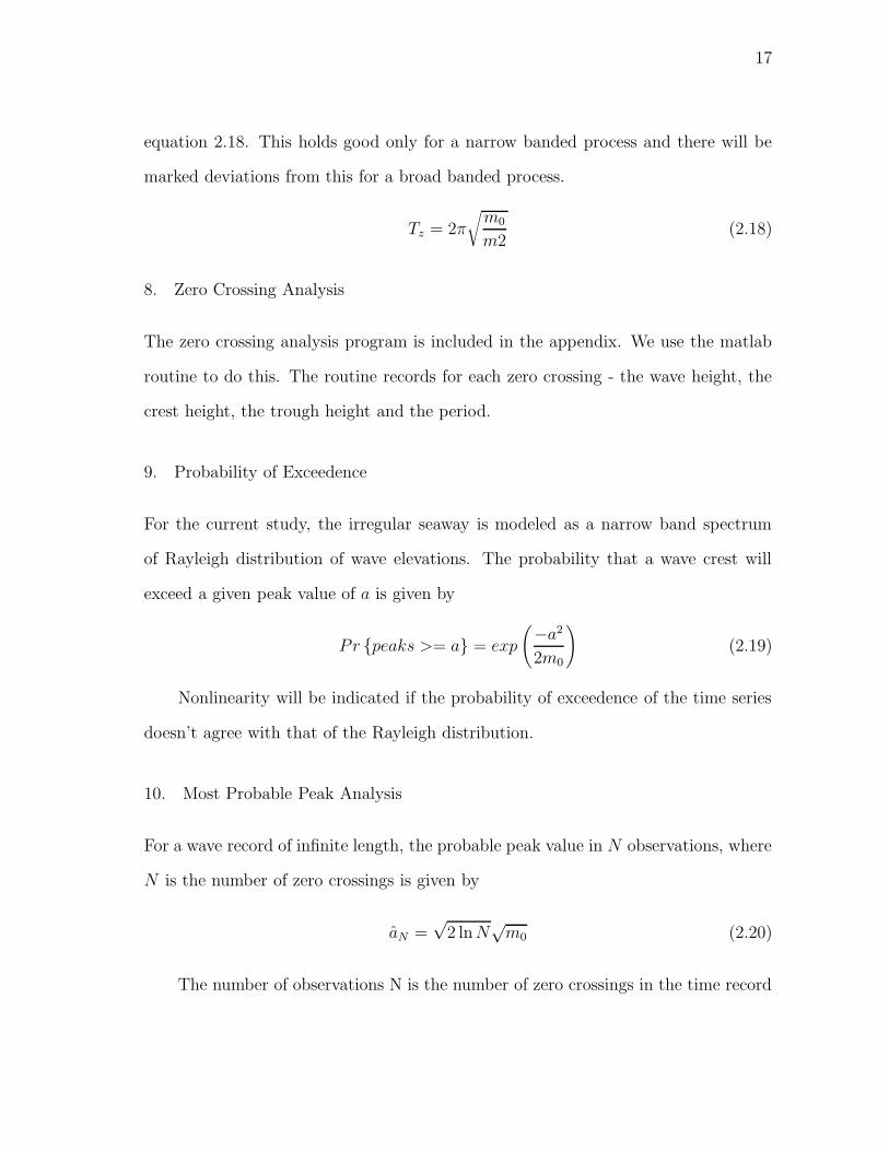
The zerocrossing period of the wave is the average time period between successive
up crossings or down crossings. For this study we will use only the zero upcrossings
periods, represented by Tz. Tz can be calculated from the spectral moments by
17
equation 2.18. This holds good only for a narrow banded process and there will be
marked deviations from this for a broad banded process.
Tz = 2π
√
m0
m2(2.18)
8. Zero Crossing Analysis
The zero crossing analysis program is included in the appendix. We use the matlab
routine to do this. The routine records for each zero crossing - the wave height, the
crest height, the trough height and the period.
9. Probability of Exceedence
For the current study, the irregular seaway is modeled as a narrow band spectrum
of Rayleigh distribution of wave elevations. The probability that a wave crest will
exceed a given peak value of a is given by
Pr {peaks >= a} = exp
(
−a2
2m0
)
(2.19)
Nonlinearity will be indicated if the probability of exceedence of the time series
doesn’t agree with that of the Rayleigh distribution.
10. Most Probable Peak Analysis
For a wave record of infinite length, the probable peak value in N observations, where
N is the number of zero crossings is given by
aN =√
2 lnN√m0 (2.20)
The number of observations N is the number of zero crossings in the time record
18
of length T.
N =T
Tz(2.21)
19
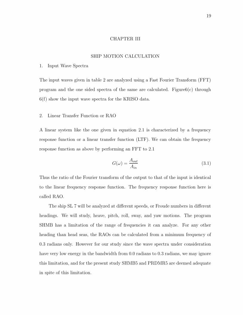
CHAPTER III
SHIP MOTION CALCULATION
1. Input Wave Spectra
The input waves given in table 2 are analyzed using a Fast Fourier Transform (FFT)
program and the one sided spectra of the same are calculated. Figure6(c) through
6(f) show the input wave spectra for the KRISO data.
2. Linear Transfer Function or RAO
A linear system like the one given in equation 2.1 is characterized by a frequency
response function or a linear transfer function (LTF). We can obtain the frequency
response function as above by performing an FFT to 2.1
G(ω) =Aout
Ain(3.1)
Thus the ratio of the Fourier transform of the output to that of the input is identical
to the linear frequency response function. The frequency response function here is
called RAO.
The ship SL 7 will be analyzed at different speeds, or Froude numbers in different
headings. We will study, heave, pitch, roll, sway, and yaw motions. The program
SHMB has a limitation of the range of frequencies it can analyze. For any other
heading than head seas, the RAOs can be calculated from a minimum frequency of
0.3 radians only. However for our study since the wave spectra under consideration
have very low energy in the bandwidth from 0.0 radians to 0.3 radians, we may ignore
this limitation, and for the present study SHMB5 and PRDMR5 are deemed adequate
in spite of this limitation.
20
0 0.1 0.2 0.3 0.4 0.5 0.6 0.7 0.8 0.9
1
0 0.2 0.4 0.6 0.8 1 1.2 1.4 1.6A
[m/m
]we [rad/s]
RAO Heading = 90 deg.
Heave motion RAO for Fn=0.00
(a) heave RAO
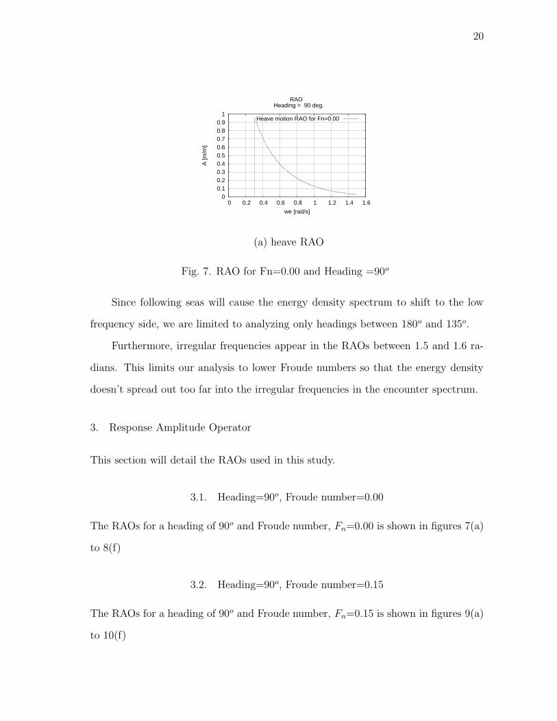
Fig. 7. RAO for Fn=0.00 and Heading =90o
Since following seas will cause the energy density spectrum to shift to the low
frequency side, we are limited to analyzing only headings between 180o and 135o.
Furthermore, irregular frequencies appear in the RAOs between 1.5 and 1.6 ra-
dians. This limits our analysis to lower Froude numbers so that the energy density
doesn’t spread out too far into the irregular frequencies in the encounter spectrum.
3. Response Amplitude Operator
This section will detail the RAOs used in this study.
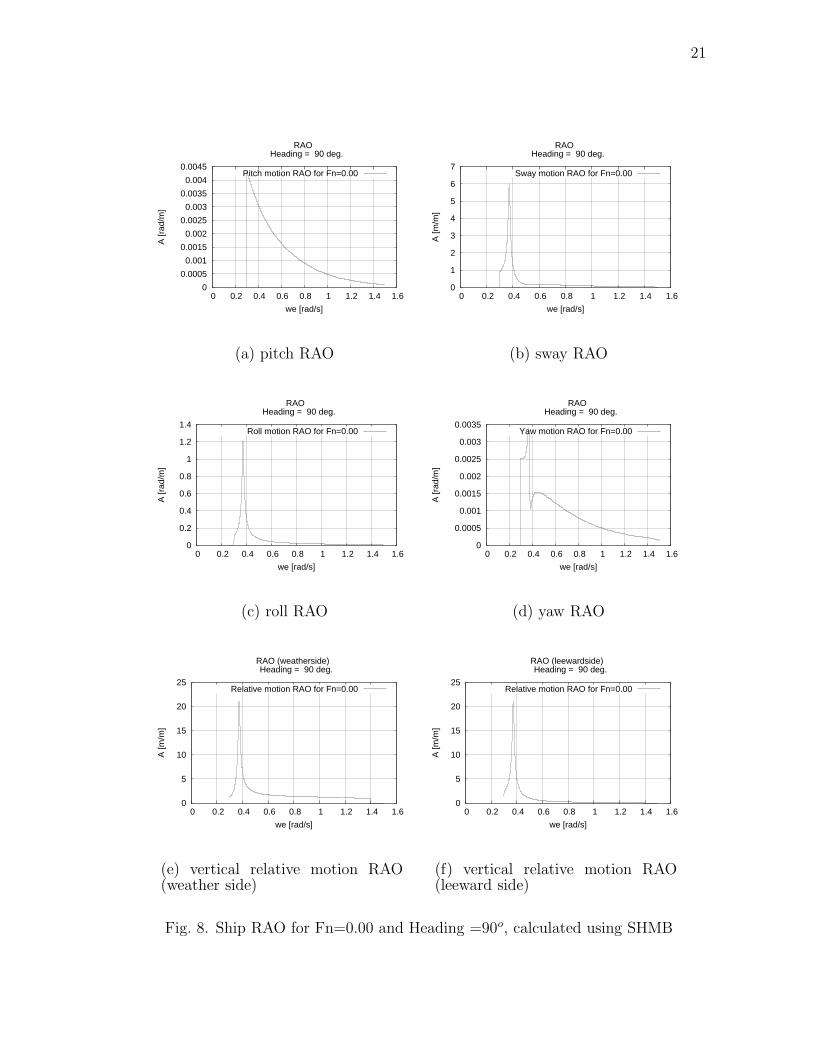
3.1. Heading=90o, Froude number=0.00
The RAOs for a heading of 90o and Froude number, Fn=0.00 is shown in figures 7(a)
to 8(f)
3.2. Heading=90o, Froude number=0.15
The RAOs for a heading of 90o and Froude number, Fn=0.15 is shown in figures 9(a)
to 10(f)
21
0
0.0005
0.001
0.0015
0.002
0.0025
0.003
0.0035
0.004
0.0045
0 0.2 0.4 0.6 0.8 1 1.2 1.4 1.6
A [r
ad/m
]
we [rad/s]
RAO Heading = 90 deg.
Pitch motion RAO for Fn=0.00
(a) pitch RAO
0
1
2
3
4
5
6
7
0 0.2 0.4 0.6 0.8 1 1.2 1.4 1.6
A [m
/m]
we [rad/s]
RAO Heading = 90 deg.
Sway motion RAO for Fn=0.00
(b) sway RAO
0
0.2
0.4
0.6
0.8
1
1.2
1.4
0 0.2 0.4 0.6 0.8 1 1.2 1.4 1.6
A [r
ad/m
]
we [rad/s]
RAO Heading = 90 deg.
Roll motion RAO for Fn=0.00
(c) roll RAO
0
0.0005
0.001
0.0015
0.002
0.0025
0.003
0.0035
0 0.2 0.4 0.6 0.8 1 1.2 1.4 1.6
A [r
ad/m
]
we [rad/s]
RAO Heading = 90 deg.
Yaw motion RAO for Fn=0.00
(d) yaw RAO
0
5
10
15
20
25
0 0.2 0.4 0.6 0.8 1 1.2 1.4 1.6
A [m
/m]
we [rad/s]
RAO (weatherside) Heading = 90 deg.
Relative motion RAO for Fn=0.00
(e) vertical relative motion RAO(weather side)
0
5
10
15
20
25
0 0.2 0.4 0.6 0.8 1 1.2 1.4 1.6
A [m
/m]
we [rad/s]
RAO (leewardside) Heading = 90 deg.
Relative motion RAO for Fn=0.00
(f) vertical relative motion RAO(leeward side)
Fig. 8. Ship RAO for Fn=0.00 and Heading =90o, calculated using SHMB
22
0 0.1 0.2 0.3 0.4 0.5 0.6 0.7 0.8 0.9
1
0 0.2 0.4 0.6 0.8 1 1.2 1.4 1.6A
[m/m
]we [rad/s]
RAO Heading = 90 deg.
Heave motion RAO for Fn=0.15
(a) heave RAO
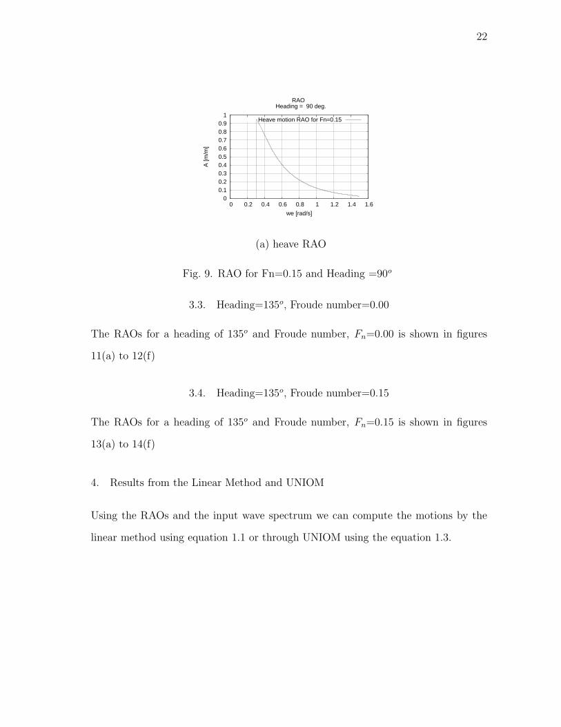
Fig. 9. RAO for Fn=0.15 and Heading =90o
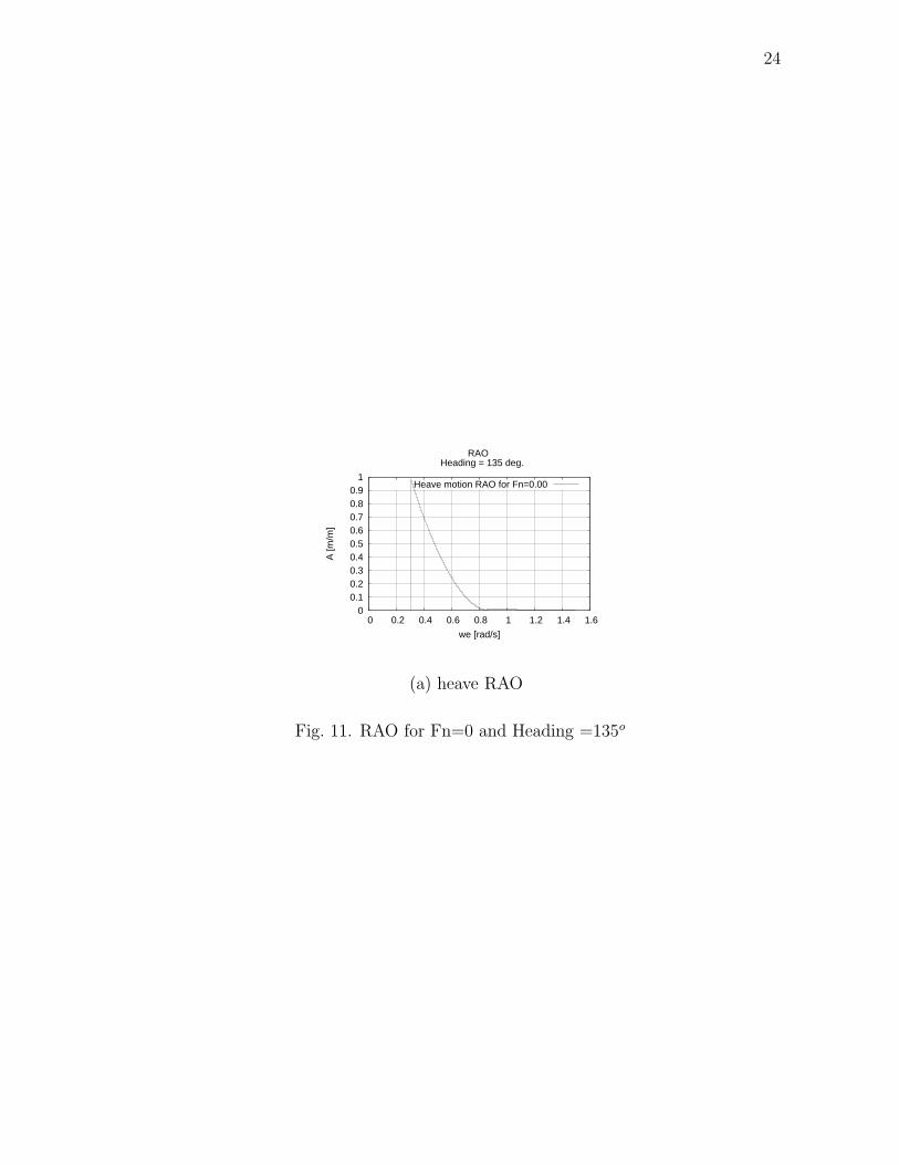
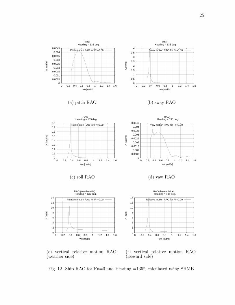
3.3. Heading=135o, Froude number=0.00
The RAOs for a heading of 135o and Froude number, Fn=0.00 is shown in figures
11(a) to 12(f)
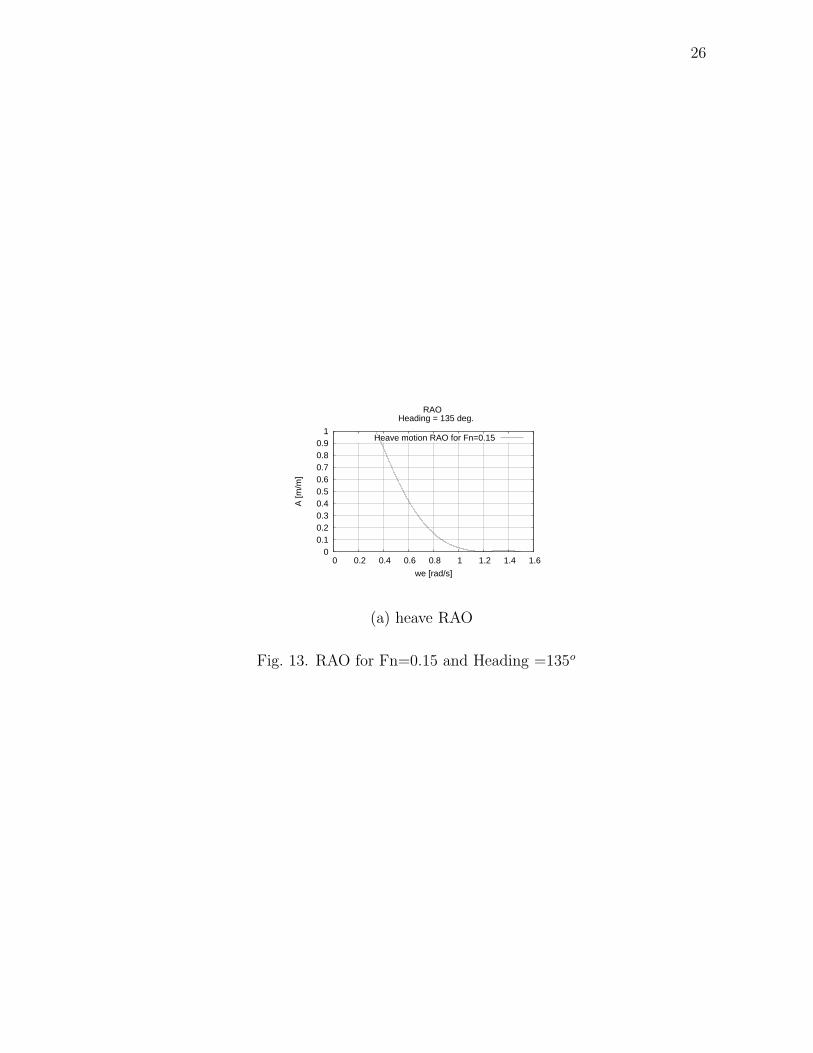
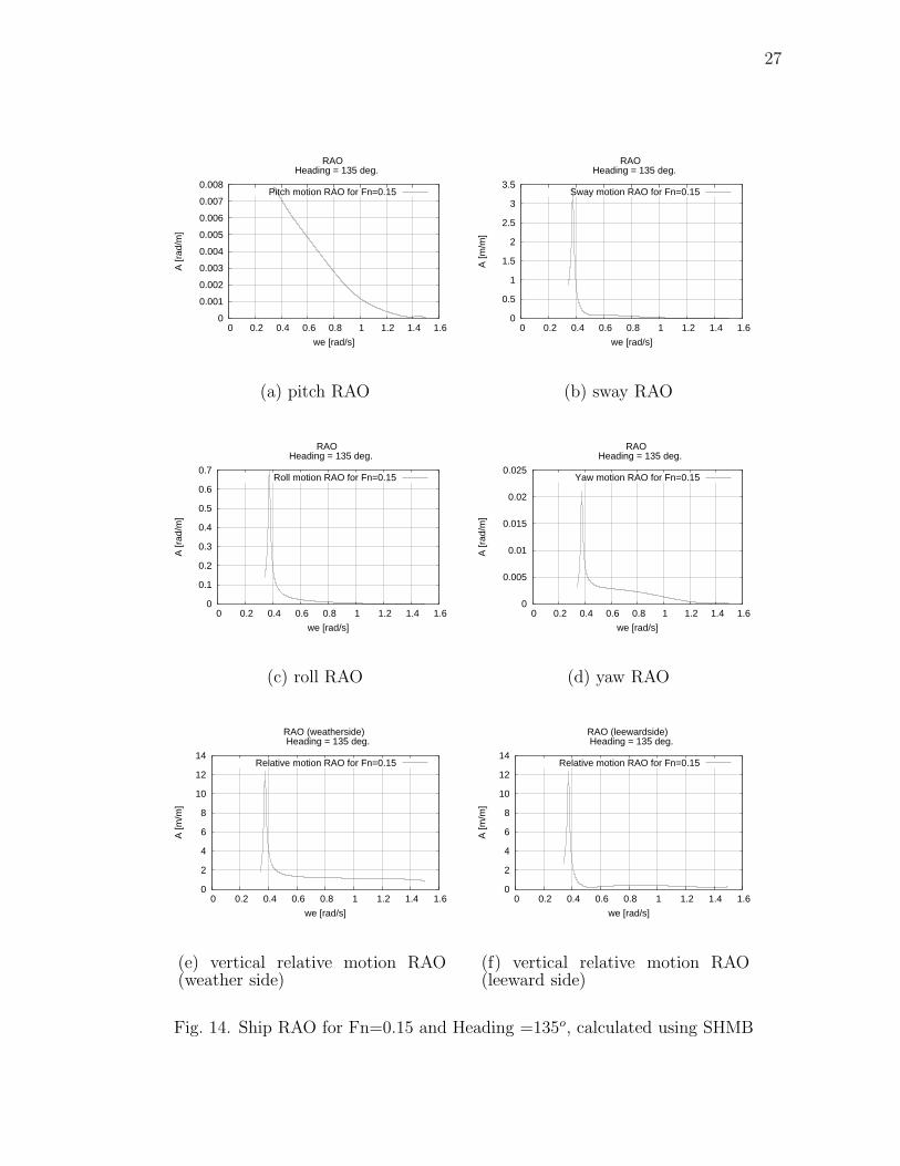
3.4. Heading=135o, Froude number=0.15
The RAOs for a heading of 135o and Froude number, Fn=0.15 is shown in figures
13(a) to 14(f)
4. Results from the Linear Method and UNIOM
Using the RAOs and the input wave spectrum we can compute the motions by the
linear method using equation 1.1 or through UNIOM using the equation 1.3.
23
0
0.001
0.002
0.003
0.004
0.005
0.006
0.007
0 0.2 0.4 0.6 0.8 1 1.2 1.4 1.6
A [r
ad/m
]
we [rad/s]
RAO Heading = 90 deg.
Pitch motion RAO for Fn=0.15
(a) pitch RAO
0
1
2
3
4
5
6
7
0 0.2 0.4 0.6 0.8 1 1.2 1.4 1.6
A [m
/m]
we [rad/s]
RAO Heading = 90 deg.
Sway motion RAO for Fn=0.15
(b) sway RAO
0
0.2
0.4
0.6
0.8
1
1.2
1.4
0 0.2 0.4 0.6 0.8 1 1.2 1.4 1.6
A [r
ad/m
]
we [rad/s]
RAO Heading = 90 deg.
Roll motion RAO for Fn=0.15
(c) roll RAO
0
0.005
0.01
0.015
0.02
0.025
0.03
0.035
0.04
0 0.2 0.4 0.6 0.8 1 1.2 1.4 1.6
A [r
ad/m
]
we [rad/s]
RAO Heading = 90 deg.
Yaw motion RAO for Fn=0.15
(d) yaw RAO
0
5
10
15
20
25
0 0.2 0.4 0.6 0.8 1 1.2 1.4 1.6
A [m
/m]
we [rad/s]
RAO (weatherside) Heading = 90 deg.
Relative motion RAO for Fn=0.15
(e) vertical relative motion RAO(weather side)
0
5
10
15
20
25
0 0.2 0.4 0.6 0.8 1 1.2 1.4 1.6
A [m
/m]
we [rad/s]
RAO (leewardside) Heading = 90 deg.
Relative motion RAO for Fn=0.15
(f) vertical relative motion RAO(leeward side)
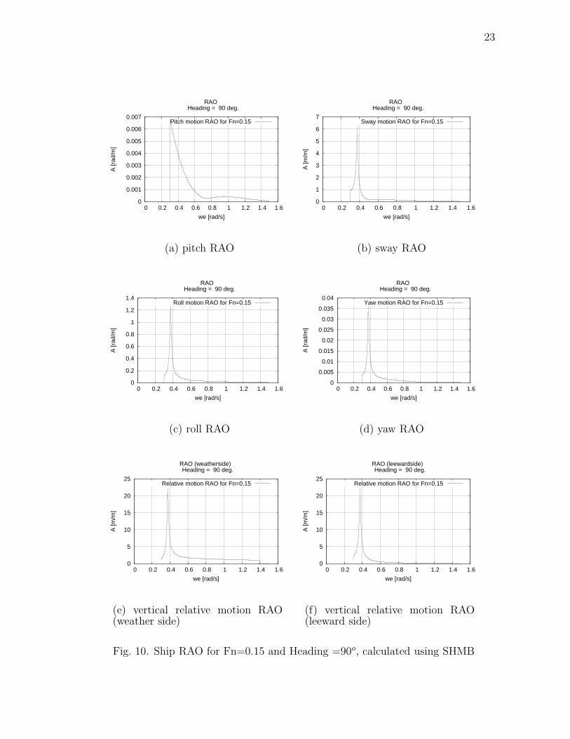
Fig. 10. Ship RAO for Fn=0.15 and Heading =90o, calculated using SHMB
24
0 0.1 0.2 0.3 0.4 0.5 0.6 0.7 0.8 0.9
1
0 0.2 0.4 0.6 0.8 1 1.2 1.4 1.6
A [m
/m]
we [rad/s]
RAO Heading = 135 deg.
Heave motion RAO for Fn=0.00
(a) heave RAO
Fig. 11. RAO for Fn=0 and Heading =135o
25
0
0.0005
0.001
0.0015
0.002
0.0025
0.003
0.0035
0.004
0.0045
0 0.2 0.4 0.6 0.8 1 1.2 1.4 1.6
A [r
ad/m
]
we [rad/s]
RAO Heading = 135 deg.
Pitch motion RAO for Fn=0.00
(a) pitch RAO
0
0.5
1
1.5
2
2.5
3
3.5
4
0 0.2 0.4 0.6 0.8 1 1.2 1.4 1.6
A [m
/m]
we [rad/s]
RAO Heading = 135 deg.
Sway motion RAO for Fn=0.00
(b) sway RAO
0
0.1
0.2
0.3
0.4
0.5
0.6
0.7
0.8
0 0.2 0.4 0.6 0.8 1 1.2 1.4 1.6
A [r
ad/m
]
we [rad/s]
RAO Heading = 135 deg.
Roll motion RAO for Fn=0.00
(c) roll RAO
0
0.0005
0.001
0.0015
0.002
0.0025
0.003
0.0035
0.004
0.0045
0 0.2 0.4 0.6 0.8 1 1.2 1.4 1.6
A [r
ad/m
]
we [rad/s]
RAO Heading = 135 deg.
Yaw motion RAO for Fn=0.00
(d) yaw RAO
0
2
4
6
8
10
12
14
0 0.2 0.4 0.6 0.8 1 1.2 1.4 1.6
A [m
/m]
we [rad/s]
RAO (weatherside) Heading = 135 deg.
Relative motion RAO for Fn=0.00
(e) vertical relative motion RAO(weather side)
0
2
4
6
8
10
12
14
0 0.2 0.4 0.6 0.8 1 1.2 1.4 1.6
A [m
/m]
we [rad/s]
RAO (leewardside) Heading = 135 deg.
Relative motion RAO for Fn=0.00
(f) vertical relative motion RAO(leeward side)
Fig. 12. Ship RAO for Fn=0 and Heading =135o, calculated using SHMB
26
0 0.1 0.2 0.3 0.4 0.5 0.6 0.7 0.8 0.9
1
0 0.2 0.4 0.6 0.8 1 1.2 1.4 1.6
A [m
/m]
we [rad/s]
RAO Heading = 135 deg.
Heave motion RAO for Fn=0.15
(a) heave RAO
Fig. 13. RAO for Fn=0.15 and Heading =135o
27
0
0.001
0.002
0.003
0.004
0.005
0.006
0.007
0.008
0 0.2 0.4 0.6 0.8 1 1.2 1.4 1.6
A [r
ad/m
]
we [rad/s]
RAO Heading = 135 deg.
Pitch motion RAO for Fn=0.15
(a) pitch RAO
0
0.5
1
1.5
2
2.5
3
3.5
0 0.2 0.4 0.6 0.8 1 1.2 1.4 1.6
A [m
/m]
we [rad/s]
RAO Heading = 135 deg.
Sway motion RAO for Fn=0.15
(b) sway RAO
0
0.1
0.2
0.3
0.4
0.5
0.6
0.7
0 0.2 0.4 0.6 0.8 1 1.2 1.4 1.6
A [r
ad/m
]
we [rad/s]
RAO Heading = 135 deg.
Roll motion RAO for Fn=0.15
(c) roll RAO
0
0.005
0.01
0.015
0.02
0.025
0 0.2 0.4 0.6 0.8 1 1.2 1.4 1.6
A [r
ad/m
]
we [rad/s]
RAO Heading = 135 deg.
Yaw motion RAO for Fn=0.15
(d) yaw RAO
0
2
4
6
8
10
12
14
0 0.2 0.4 0.6 0.8 1 1.2 1.4 1.6
A [m
/m]
we [rad/s]
RAO (weatherside) Heading = 135 deg.
Relative motion RAO for Fn=0.15
(e) vertical relative motion RAO(weather side)
0
2
4
6
8
10
12
14
0 0.2 0.4 0.6 0.8 1 1.2 1.4 1.6
A [m
/m]
we [rad/s]
RAO (leewardside) Heading = 135 deg.
Relative motion RAO for Fn=0.15
(f) vertical relative motion RAO(leeward side)
Fig. 14. Ship RAO for Fn=0.15 and Heading =135o, calculated using SHMB
28
CHAPTER IV
ANALYSIS RESULTS FOR HEADING = 90O AND FN = 0.00
The motions of the container ship SL 7 for Fn = 0 and headings of 90o are calculated
using the linear approach and using UNIOM.
1. Simulation Results
In this section, the results from using the linear theory and UNIOM are compared.
The simulation using UNIOM is carried out for 3600 seconds, but for the plots to be
readable, only 1500 seconds of data is shown. The time steps used for the simulations
is 1 second. The peak values are found corresponding to a time duration of 3600
seconds.
2. Probability of Exceedence
The probability of exceedence for the wave as well as the response motions are cal-
culated. The following pages show the input wave and the responses.
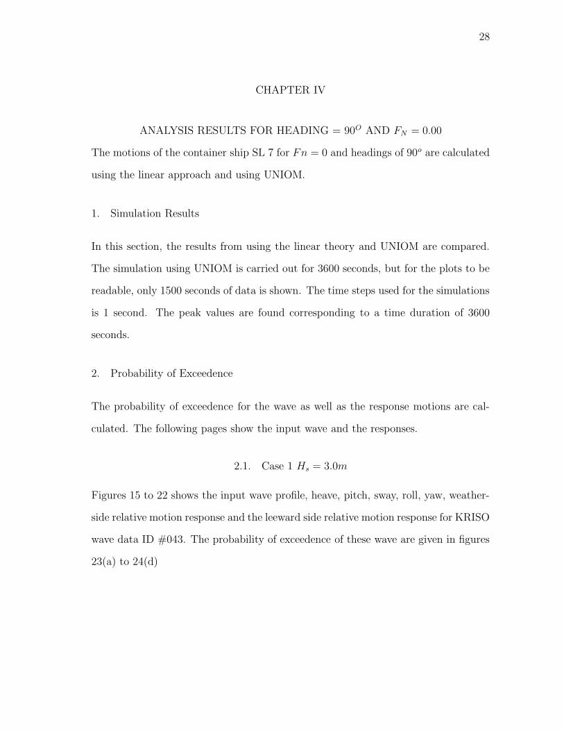
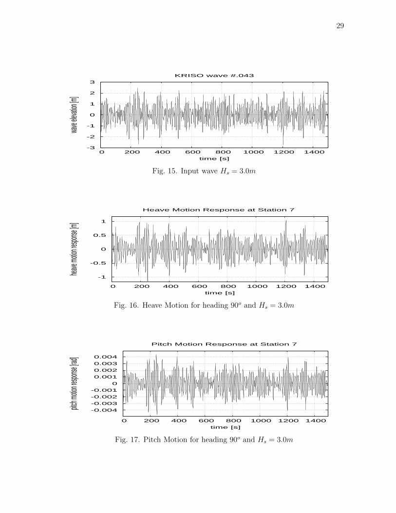
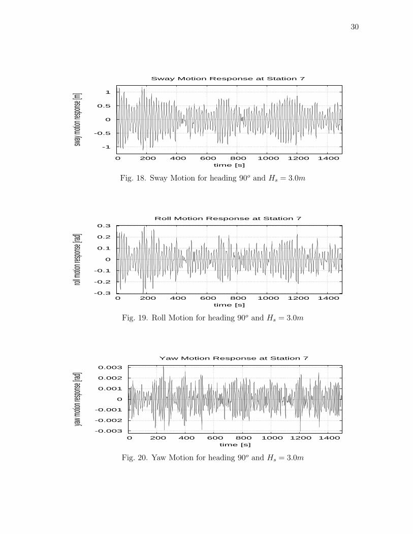
2.1. Case 1 Hs = 3.0m
Figures 15 to 22 shows the input wave profile, heave, pitch, sway, roll, yaw, weather-
side relative motion response and the leeward side relative motion response for KRISO
wave data ID #043. The probability of exceedence of these wave are given in figures
23(a) to 24(d)
29
-3
-2
-1
0
1
2
3
0 200 400 600 800 1000 1200 1400
wave
elevat
ion [m
]
time [s]
KRISO wave #.043
Fig. 15. Input wave Hs = 3.0m
-1
-0.5
0
0.5
1
0 200 400 600 800 1000 1200 1400
heave
motion
respon
se [m]
time [s]
Heave Motion Response at Station 7
Fig. 16. Heave Motion for heading 90o and Hs = 3.0m
-0.004
-0.003
-0.002
-0.001
0
0.001
0.002
0.003
0.004
0 200 400 600 800 1000 1200 1400
pitch m
otion re
sponse
[rad]
time [s]
Pitch Motion Response at Station 7
Fig. 17. Pitch Motion for heading 90o and Hs = 3.0m
30
-1
-0.5
0
0.5
1
0 200 400 600 800 1000 1200 1400
sway m
otion re
sponse
[m]
time [s]
Sway Motion Response at Station 7
Fig. 18. Sway Motion for heading 90o and Hs = 3.0m
-0.3
-0.2
-0.1
0
0.1
0.2
0.3
0 200 400 600 800 1000 1200 1400
roll mo
tion res
ponse
[rad]
time [s]
Roll Motion Response at Station 7
Fig. 19. Roll Motion for heading 90o and Hs = 3.0m
-0.003
-0.002
-0.001
0
0.001
0.002
0.003
0 200 400 600 800 1000 1200 1400
yaw mo
tion res
ponse
[rad]
time [s]
Yaw Motion Response at Station 7
Fig. 20. Yaw Motion for heading 90o and Hs = 3.0m
31
-6
-4
-2
0
2
4
6
0 200 400 600 800 1000 1200 1400
relative
motion
respon
se [m]
time [s]
weather side relative motion response at station 7
Fig. 21. Relative Motion at weather side for heading 90o and Hs = 3.0m
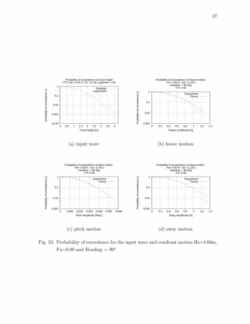
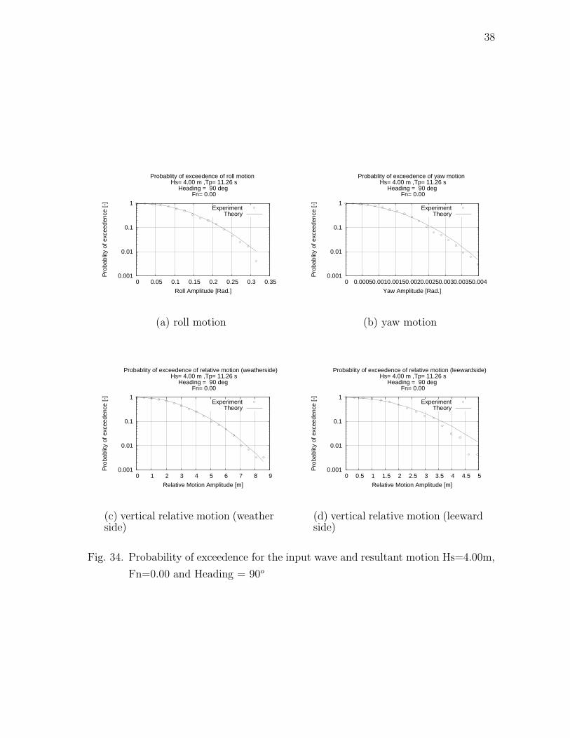
2.2. Case 2 Hs = 4.0m
Figures 25 to 32 shows the input wave profile, heave, pitch, sway, roll, yaw,weatherside
relative motion response and the leeward side relative motion response for KRISO
wave data ID #042.The probability of exceedence of these wave are given in figures
33(a) to 34(d)
-4
-2
0
2
4
0 200 400 600 800 1000 1200 1400
relative
motion
respon
se [m]
time [s]
leeward side relative motion response at station 7
Fig. 22. Relative Motion at leeward side for heading 90o and Hs = 3.0m
32
1e-04
0.001
0.01
0.1
1
0 0.5 1 1.5 2 2.5
prob
ablit
y of
exc
eede
nce
[-]
Crest height [m]
Probablity of exceedence of crest heightITTC Hs= 3.00 m ,Tp= 11.26 s gamma= 1.00
Rayleighexperiment
(a) Input wave
0.001
0.01
0.1
1
0 0.2 0.4 0.6 0.8 1 1.2
Pro
babl
ity o
f exc
eede
nce
[-]
Heave Amplitude [m]
Probablity of exceedence of heave motion Hs= 3.00 m ,Tp= 11.26 s
Heading = 90 deg Fn= 0.00
ExperimentTheory
(b) Heave motion
0.001
0.01
0.1
1
0 0.0005 0.001 0.0015 0.002 0.0025 0.003 0.0035 0.004 0.0045
Pro
babl
ity o
f exc
eede
nce
[-]
Pitch Amplitude [Rad.]
Probablity of exceedence of pitch motion Hs= 3.00 m ,Tp= 11.26 s
Heading = 90 deg Fn= 0.00
ExperimentTheory
(c) Pitch motion
0.001
0.01
0.1
1
0 0.2 0.4 0.6 0.8 1 1.2 1.4
Pro
babl
ity o
f exc
eede
nce
[-]
Sway Amplitude [m]
Probablity of exceedence of sway motion Hs= 3.00 m ,Tp= 11.26 s
Heading = 90 deg Fn= 0.00
ExperimentTheory
(d) Sway motion
Fig. 23. Probability of exceedence for the input wave and resultant motion Hs=3.00m,
Fn=0.00 and Heading = 90o

33
0.001
0.01
0.1
1
0 0.05 0.1 0.15 0.2 0.25 0.3
Pro
babl
ity o
f exc
eede
nce
[-]
Roll Amplitude [Rad.]
Probablity of exceedence of roll motion Hs= 3.00 m ,Tp= 11.26 s
Heading = 90 deg Fn= 0.00
ExperimentTheory
(a) Roll motion
0.001
0.01
0.1
1
0 0.0005 0.001 0.0015 0.002 0.0025 0.003 0.0035
Pro
babl
ity o
f exc
eede
nce
[-]
Yaw Amplitude [Rad.]
Probablity of exceedence of yaw motion Hs= 3.00 m ,Tp= 11.26 s
Heading = 90 deg Fn= 0.00
ExperimentTheory
(b) Yaw motion
0.001
0.01
0.1
1
0 1 2 3 4 5 6 7
Pro
babl
ity o
f exc
eede
nce
[-]
Relative Motion Amplitude [m]
Probablity of exceedence of relative motion (weatherside) Hs= 3.00 m ,Tp= 11.26 s
Heading = 90 deg Fn= 0.00
ExperimentTheory
(c) vertical relative motion (weatherside)
0.001
0.01
0.1
1
0 0.5 1 1.5 2 2.5 3 3.5 4 4.5
Pro
babl
ity o
f exc
eede
nce
[-]
Relative Motion Amplitude [m]
Probablity of exceedence of relative motion (leewardside) Hs= 3.00 m ,Tp= 11.26 s
Heading = 90 deg Fn= 0.00
ExperimentTheory
(d) vertical relative motion (leewardside)
Fig. 24. Probability of exceedence for the input wave and resultant motion Hs=3.00m,
Fn=0.00 and Heading = 90o
34
-4
-3
-2
-1
0
1
2
3
4
0 200 400 600 800 1000 1200 1400
wave
elevat
ion [m
]
time [s]
KRISO wave #.042
Fig. 25. Input wave Hs = 4.0m
-1.5
-1
-0.5
0
0.5
1
1.5
0 200 400 600 800 1000 1200 1400
heave
motion
respon
se [m]
time [s]
Heave Motion Response at Station 7
Fig. 26. Heave Motion for heading 90o and Hs = 4.0m
-0.006
-0.004
-0.002
0
0.002
0.004
0.006
0 200 400 600 800 1000 1200 1400
pitch m
otion re
sponse
[rad]
time [s]
Pitch Motion Response at Station 7
Fig. 27. Pitch Motion for heading 90o and Hs = 4.0m
35
-1
-0.5
0
0.5
1
0 200 400 600 800 1000 1200 1400
sway m
otion re
sponse
[m]
time [s]
Sway Motion Response at Station 7
Fig. 28. Sway Motion for heading 90o and Hs = 4.0m
-0.3
-0.2
-0.1
0
0.1
0.2
0.3
0 200 400 600 800 1000 1200 1400
roll mo
tion res
ponse
[rad]
time [s]
Roll Motion Response at Station 7
Fig. 29. Roll Motion for heading 90o and Hs = 4.0m
-0.004
-0.003
-0.002
-0.001
0
0.001
0.002
0.003
0.004
0 200 400 600 800 1000 1200 1400
yaw mo
tion res
ponse
[rad]
time [s]
Yaw Motion Response at Station 7
Fig. 30. Yaw Motion for heading 90o and Hs = 4.0m
36
-8
-6
-4
-2
0
2
4
6
8
0 200 400 600 800 1000 1200 1400
relative
motion
respon
se [m]
time [s]
weather side relative motion response at station 7
Fig. 31. Relative Motion at weather side for heading 90o and Hs = 4.0m
-4
-2
0
2
4
0 200 400 600 800 1000 1200 1400
relative
motion
respon
se [m]
time [s]
leeward side relative motion response at station 7
Fig. 32. Relative Motion at leeward side for heading 90o and Hs = 4.0m
37
1e-04
0.001
0.01
0.1
1
0 0.5 1 1.5 2 2.5 3 3.5 4
prob
ablit
y of
exc
eede
nce
[-]
Crest height [m]
Probablity of exceedence of crest heightITTC Hs= 4.00 m ,Tp= 11.26 s gamma= 1.00
Rayleighexperiment
(a) input wave
0.001
0.01
0.1
1
0 0.2 0.4 0.6 0.8 1 1.2 1.4
Pro
babl
ity o
f exc
eede
nce
[-]
Heave Amplitude [m]
Probablity of exceedence of heave motion Hs= 4.00 m ,Tp= 11.26 s
Heading = 90 deg Fn= 0.00
ExperimentTheory
(b) heave motion
0.001
0.01
0.1
1
0 0.001 0.002 0.003 0.004 0.005 0.006
Pro
babl
ity o
f exc
eede
nce
[-]
Pitch Amplitude [Rad.]
Probablity of exceedence of pitch motion Hs= 4.00 m ,Tp= 11.26 s
Heading = 90 deg Fn= 0.00
ExperimentTheory
(c) pitch motion
0.001
0.01
0.1
1
0 0.2 0.4 0.6 0.8 1 1.2 1.4
Pro
babl
ity o
f exc
eede
nce
[-]
Sway Amplitude [m]
Probablity of exceedence of sway motion Hs= 4.00 m ,Tp= 11.26 s
Heading = 90 deg Fn= 0.00
ExperimentTheory
(d) sway motion
Fig. 33. Probability of exceedence for the input wave and resultant motion Hs=4.00m,
Fn=0.00 and Heading = 90o
38
0.001
0.01
0.1
1
0 0.05 0.1 0.15 0.2 0.25 0.3 0.35
Pro
babl
ity o
f exc
eede
nce
[-]
Roll Amplitude [Rad.]
Probablity of exceedence of roll motion Hs= 4.00 m ,Tp= 11.26 s
Heading = 90 deg Fn= 0.00
ExperimentTheory
(a) roll motion
0.001
0.01
0.1
1
0 0.0005 0.001 0.0015 0.002 0.0025 0.003 0.0035 0.004
Pro
babl
ity o
f exc
eede
nce
[-]
Yaw Amplitude [Rad.]
Probablity of exceedence of yaw motion Hs= 4.00 m ,Tp= 11.26 s
Heading = 90 deg Fn= 0.00
ExperimentTheory
(b) yaw motion
0.001
0.01
0.1
1
0 1 2 3 4 5 6 7 8 9
Pro
babl
ity o
f exc
eede
nce
[-]
Relative Motion Amplitude [m]
Probablity of exceedence of relative motion (weatherside) Hs= 4.00 m ,Tp= 11.26 s
Heading = 90 deg Fn= 0.00
ExperimentTheory
(c) vertical relative motion (weatherside)
0.001
0.01
0.1
1
0 0.5 1 1.5 2 2.5 3 3.5 4 4.5 5
Pro
babl
ity o
f exc
eede
nce
[-]
Relative Motion Amplitude [m]
Probablity of exceedence of relative motion (leewardside) Hs= 4.00 m ,Tp= 11.26 s
Heading = 90 deg Fn= 0.00
ExperimentTheory
(d) vertical relative motion (leewardside)
Fig. 34. Probability of exceedence for the input wave and resultant motion Hs=4.00m,
Fn=0.00 and Heading = 90o
39
-6
-4
-2
0
2
4
6
0 200 400 600 800 1000 1200 1400
wave
elevat
ion [m
]
time [s]
KRISO wave #.010
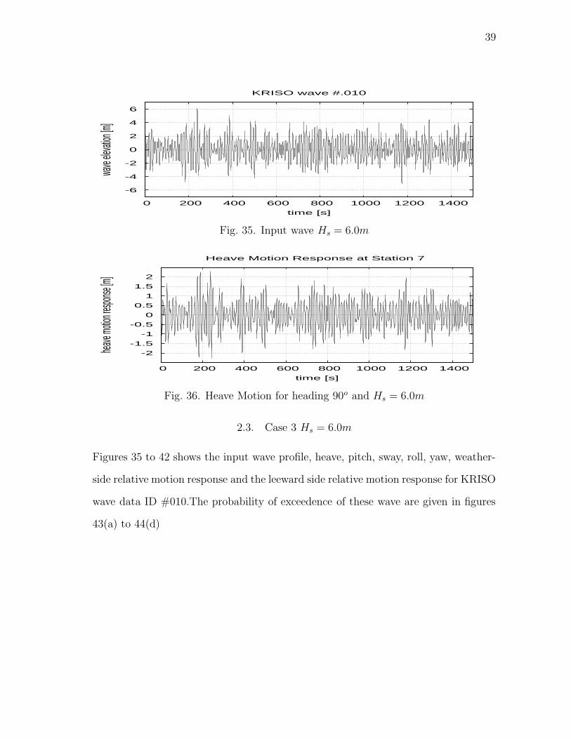
Fig. 35. Input wave Hs = 6.0m
-2
-1.5
-1
-0.5
0
0.5
1
1.5
2
0 200 400 600 800 1000 1200 1400
heave
motion
respon
se [m]
time [s]
Heave Motion Response at Station 7
Fig. 36. Heave Motion for heading 90o and Hs = 6.0m
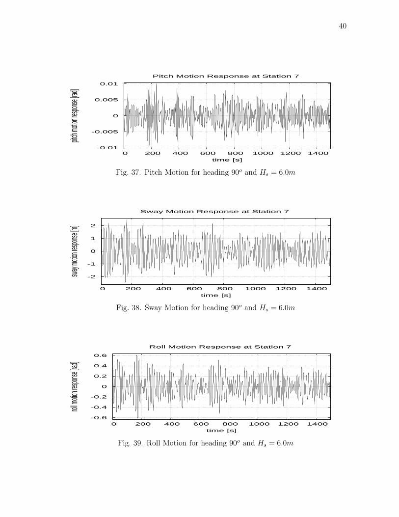
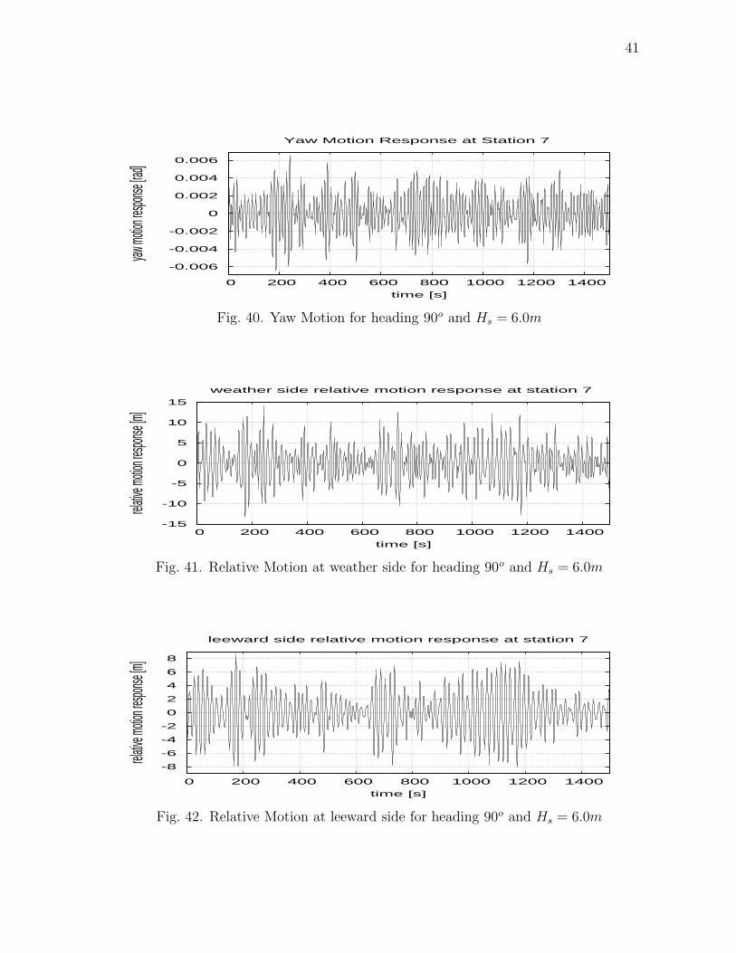
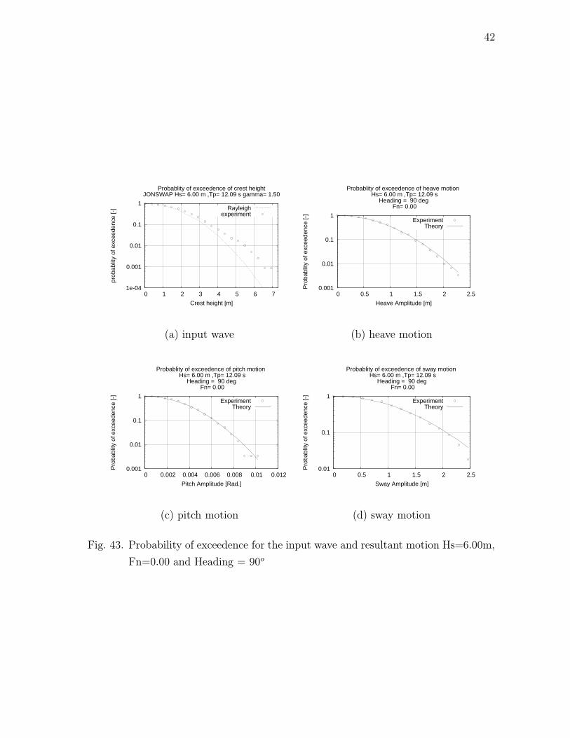
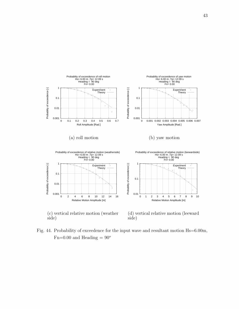
2.3. Case 3 Hs = 6.0m
Figures 35 to 42 shows the input wave profile, heave, pitch, sway, roll, yaw, weather-
side relative motion response and the leeward side relative motion response for KRISO
wave data ID #010.The probability of exceedence of these wave are given in figures
43(a) to 44(d)
40
-0.01
-0.005
0
0.005
0.01
0 200 400 600 800 1000 1200 1400
pitch m
otion re
sponse
[rad]
time [s]
Pitch Motion Response at Station 7
Fig. 37. Pitch Motion for heading 90o and Hs = 6.0m
-2
-1
0
1
2
0 200 400 600 800 1000 1200 1400
sway m
otion re
sponse
[m]
time [s]
Sway Motion Response at Station 7
Fig. 38. Sway Motion for heading 90o and Hs = 6.0m
-0.6
-0.4
-0.2
0
0.2
0.4
0.6
0 200 400 600 800 1000 1200 1400
roll mo
tion res
ponse
[rad]
time [s]
Roll Motion Response at Station 7
Fig. 39. Roll Motion for heading 90o and Hs = 6.0m
41
-0.006
-0.004
-0.002
0
0.002
0.004
0.006
0 200 400 600 800 1000 1200 1400
yaw mo
tion res
ponse
[rad]
time [s]
Yaw Motion Response at Station 7
Fig. 40. Yaw Motion for heading 90o and Hs = 6.0m
-15
-10
-5
0
5
10
15
0 200 400 600 800 1000 1200 1400
relative
motion
respon
se [m]
time [s]
weather side relative motion response at station 7
Fig. 41. Relative Motion at weather side for heading 90o and Hs = 6.0m
-8
-6
-4
-2
0
2
4
6
8
0 200 400 600 800 1000 1200 1400
relative
motion
respon
se [m]
time [s]
leeward side relative motion response at station 7
Fig. 42. Relative Motion at leeward side for heading 90o and Hs = 6.0m
42
1e-04
0.001
0.01
0.1
1
0 1 2 3 4 5 6 7
prob
ablit
y of
exc
eede
nce
[-]
Crest height [m]
Probablity of exceedence of crest heightJONSWAP Hs= 6.00 m ,Tp= 12.09 s gamma= 1.50
Rayleighexperiment
(a) input wave
0.001
0.01
0.1
1
0 0.5 1 1.5 2 2.5
Pro
babl
ity o
f exc
eede
nce
[-]
Heave Amplitude [m]
Probablity of exceedence of heave motion Hs= 6.00 m ,Tp= 12.09 s
Heading = 90 deg Fn= 0.00
ExperimentTheory
(b) heave motion
0.001
0.01
0.1
1
0 0.002 0.004 0.006 0.008 0.01 0.012
Pro
babl
ity o
f exc
eede
nce
[-]
Pitch Amplitude [Rad.]
Probablity of exceedence of pitch motion Hs= 6.00 m ,Tp= 12.09 s
Heading = 90 deg Fn= 0.00
ExperimentTheory
(c) pitch motion
0.01
0.1
1
0 0.5 1 1.5 2 2.5
Pro
babl
ity o
f exc
eede
nce
[-]
Sway Amplitude [m]
Probablity of exceedence of sway motion Hs= 6.00 m ,Tp= 12.09 s
Heading = 90 deg Fn= 0.00
ExperimentTheory
(d) sway motion
Fig. 43. Probability of exceedence for the input wave and resultant motion Hs=6.00m,
Fn=0.00 and Heading = 90o
43
0.001
0.01
0.1
1
0 0.1 0.2 0.3 0.4 0.5 0.6 0.7
Pro
babl
ity o
f exc
eede
nce
[-]
Roll Amplitude [Rad.]
Probablity of exceedence of roll motion Hs= 6.00 m ,Tp= 12.09 s
Heading = 90 deg Fn= 0.00
ExperimentTheory
(a) roll motion
0.001
0.01
0.1
1
0 0.001 0.002 0.003 0.004 0.005 0.006 0.007
Pro
babl
ity o
f exc
eede
nce
[-]
Yaw Amplitude [Rad.]
Probablity of exceedence of yaw motion Hs= 6.00 m ,Tp= 12.09 s
Heading = 90 deg Fn= 0.00
ExperimentTheory
(b) yaw motion
0.001
0.01
0.1
1
0 2 4 6 8 10 12 14 16
Pro
babl
ity o
f exc
eede
nce
[-]
Relative Motion Amplitude [m]
Probablity of exceedence of relative motion (weatherside) Hs= 6.00 m ,Tp= 12.09 s
Heading = 90 deg Fn= 0.00
ExperimentTheory
(c) vertical relative motion (weatherside)
0.01
0.1
1
0 1 2 3 4 5 6 7 8 9 10
Pro
babl
ity o
f exc
eede
nce
[-]
Relative Motion Amplitude [m]
Probablity of exceedence of relative motion (leewardside) Hs= 6.00 m ,Tp= 12.09 s
Heading = 90 deg Fn= 0.00
ExperimentTheory
(d) vertical relative motion (leewardside)
Fig. 44. Probability of exceedence for the input wave and resultant motion Hs=6.00m,
Fn=0.00 and Heading = 90o

44
-8
-6
-4
-2
0
2
4
6
8
0 200 400 600 800 1000 1200 1400
wave
elevat
ion [m
]
time [s]
KRISO wave #.014
Fig. 45. Input wave Hs = 7.0m
-3
-2
-1
0
1
2
3
0 200 400 600 800 1000 1200 1400
heave
motion
respon
se [m]
time [s]
Heave Motion Response at Station 7
Fig. 46. Heave Motion for heading 90o and Hs = 7.0m
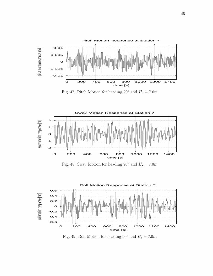
2.4. Case 4 Hs = 7.0m
Figures 45 to 52 shows the input wave profile, heave, pitch, sway, roll, yaw, weather-
side relative motion response and the leeward side relative motion response for KRISO
wave data ID #014.The probability of exceedence of these wave are given in figures
53(a) to 54(d)
45
-0.01
-0.005
0
0.005
0.01
0 200 400 600 800 1000 1200 1400
pitch m
otion re
sponse
[rad]
time [s]
Pitch Motion Response at Station 7
Fig. 47. Pitch Motion for heading 90o and Hs = 7.0m
-2
-1
0
1
2
0 200 400 600 800 1000 1200 1400
sway m
otion re
sponse
[m]
time [s]
Sway Motion Response at Station 7
Fig. 48. Sway Motion for heading 90o and Hs = 7.0m
-0.6
-0.4
-0.2
0
0.2
0.4
0.6
0 200 400 600 800 1000 1200 1400
roll mo
tion res
ponse
[rad]
time [s]
Roll Motion Response at Station 7
Fig. 49. Roll Motion for heading 90o and Hs = 7.0m
46
-0.008
-0.006
-0.004
-0.002
0
0.002
0.004
0.006
0.008
0 200 400 600 800 1000 1200 1400
yaw mo
tion res
ponse
[rad]
time [s]
Yaw Motion Response at Station 7
Fig. 50. Yaw Motion for heading 90o and Hs = 7.0m
-15
-10
-5
0
5
10
15
0 200 400 600 800 1000 1200 1400
relative
motion
respon
se [m]
time [s]
weather side relative motion response at station 7
Fig. 51. Relative Motion at weather side for heading 90o and Hs = 7.0m
-10
-5
0
5
10
0 200 400 600 800 1000 1200 1400
relative
motion
respon
se [m]
time [s]
leeward side relative motion response at station 7
Fig. 52. Relative Motion at leeward side for heading 90o and Hs = 7.0m
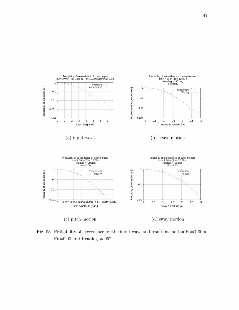
47
1e-04
0.001
0.01
0.1
1
0 1 2 3 4 5 6 7
prob
ablit
y of
exc
eede
nce
[-]
Crest height [m]
Probablity of exceedence of crest heightJONSWAP Hs= 7.00 m ,Tp= 12.09 s gamma= 2.00
Rayleighexperiment
(a) input wave
0.001
0.01
0.1
1
0 0.5 1 1.5 2 2.5 3
Pro
babl
ity o
f exc
eede
nce
[-]
Heave Amplitude [m]
Probablity of exceedence of heave motion Hs= 7.00 m ,Tp= 12.09 s
Heading = 90 deg Fn= 0.00
ExperimentTheory
(b) heave motion
0.001
0.01
0.1
1
0 0.002 0.004 0.006 0.008 0.01 0.012 0.014
Pro
babl
ity o
f exc
eede
nce
[-]
Pitch Amplitude [Rad.]
Probablity of exceedence of pitch motion Hs= 7.00 m ,Tp= 12.09 s
Heading = 90 deg Fn= 0.00
ExperimentTheory
(c) pitch motion
0.01
0.1
1
0 0.5 1 1.5 2 2.5 3
Pro
babl
ity o
f exc
eede
nce
[-]
Sway Amplitude [m]
Probablity of exceedence of sway motion Hs= 7.00 m ,Tp= 12.09 s
Heading = 90 deg Fn= 0.00
ExperimentTheory
(d) sway motion
Fig. 53. Probability of exceedence for the input wave and resultant motion Hs=7.00m,
Fn=0.00 and Heading = 90o
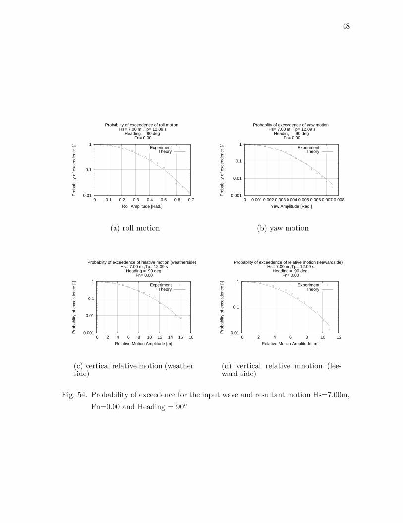
48
0.01
0.1
1
0 0.1 0.2 0.3 0.4 0.5 0.6 0.7
Pro
babl
ity o
f exc
eede
nce
[-]
Roll Amplitude [Rad.]
Probablity of exceedence of roll motion Hs= 7.00 m ,Tp= 12.09 s
Heading = 90 deg Fn= 0.00
ExperimentTheory
(a) roll motion
0.001
0.01
0.1
1
0 0.001 0.002 0.003 0.004 0.005 0.006 0.007 0.008
Pro
babl
ity o
f exc
eede
nce
[-]
Yaw Amplitude [Rad.]
Probablity of exceedence of yaw motion Hs= 7.00 m ,Tp= 12.09 s
Heading = 90 deg Fn= 0.00
ExperimentTheory
(b) yaw motion
0.001
0.01
0.1
1
0 2 4 6 8 10 12 14 16 18
Pro
babl
ity o
f exc
eede
nce
[-]
Relative Motion Amplitude [m]
Probablity of exceedence of relative motion (weatherside) Hs= 7.00 m ,Tp= 12.09 s
Heading = 90 deg Fn= 0.00
ExperimentTheory
(c) vertical relative motion (weatherside)
0.01
0.1
1
0 2 4 6 8 10 12
Pro
babl
ity o
f exc
eede
nce
[-]
Relative Motion Amplitude [m]
Probablity of exceedence of relative motion (leewardside) Hs= 7.00 m ,Tp= 12.09 s
Heading = 90 deg Fn= 0.00
ExperimentTheory
(d) vertical relative mnotion (lee-ward side)
Fig. 54. Probability of exceedence for the input wave and resultant motion Hs=7.00m,
Fn=0.00 and Heading = 90o
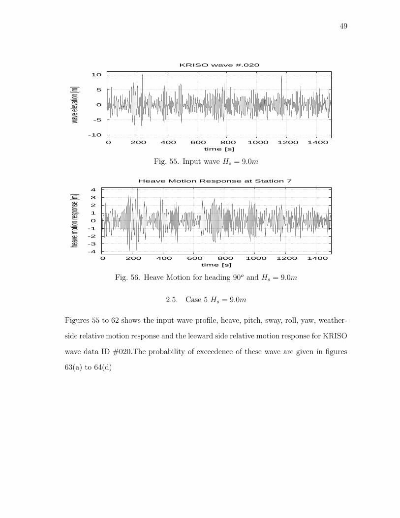
49
-10
-5
0
5
10
0 200 400 600 800 1000 1200 1400
wave
elevat
ion [m
]
time [s]
KRISO wave #.020
Fig. 55. Input wave Hs = 9.0m
-4
-3
-2
-1
0
1
2
3
4
0 200 400 600 800 1000 1200 1400
heave
motion
respon
se [m]
time [s]
Heave Motion Response at Station 7
Fig. 56. Heave Motion for heading 90o and Hs = 9.0m
2.5. Case 5 Hs = 9.0m
Figures 55 to 62 shows the input wave profile, heave, pitch, sway, roll, yaw, weather-
side relative motion response and the leeward side relative motion response for KRISO
wave data ID #020.The probability of exceedence of these wave are given in figures
63(a) to 64(d)
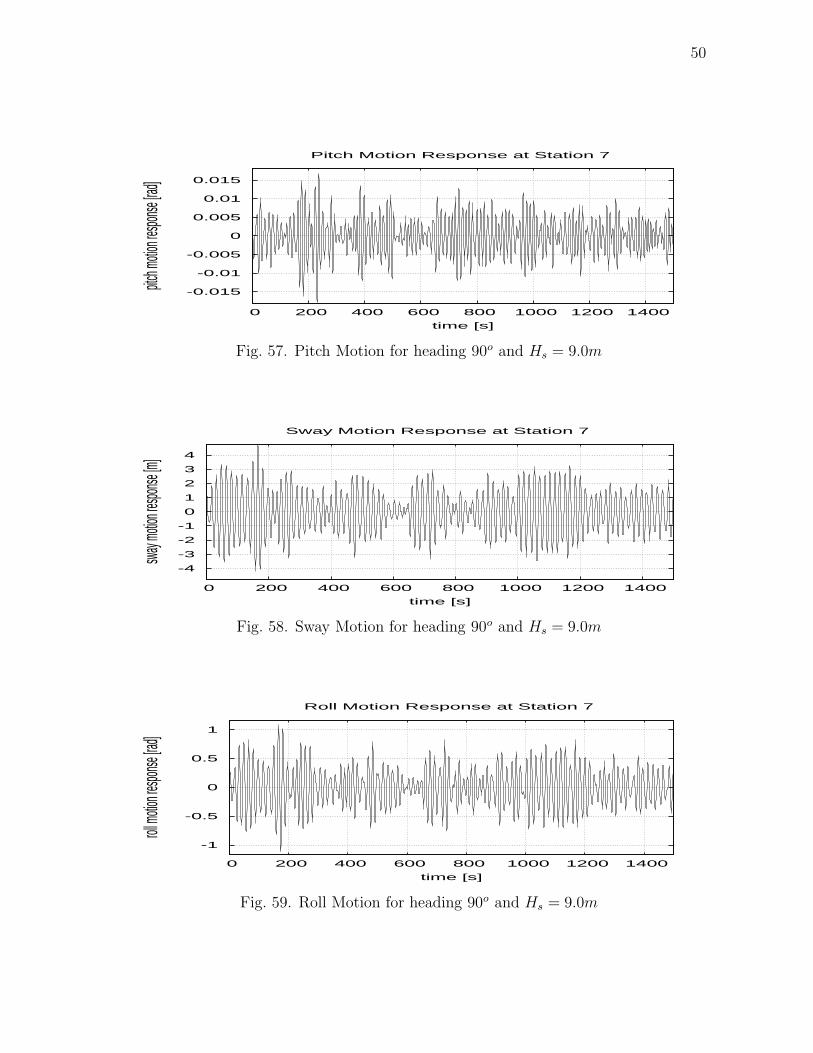
50
-0.015
-0.01
-0.005
0
0.005
0.01
0.015
0 200 400 600 800 1000 1200 1400
pitch m
otion re
sponse
[rad]
time [s]
Pitch Motion Response at Station 7
Fig. 57. Pitch Motion for heading 90o and Hs = 9.0m
-4
-3
-2
-1
0
1
2
3
4
0 200 400 600 800 1000 1200 1400
sway m
otion re
sponse
[m]
time [s]
Sway Motion Response at Station 7
Fig. 58. Sway Motion for heading 90o and Hs = 9.0m
-1
-0.5
0
0.5
1
0 200 400 600 800 1000 1200 1400
roll mo
tion res
ponse
[rad]
time [s]
Roll Motion Response at Station 7
Fig. 59. Roll Motion for heading 90o and Hs = 9.0m
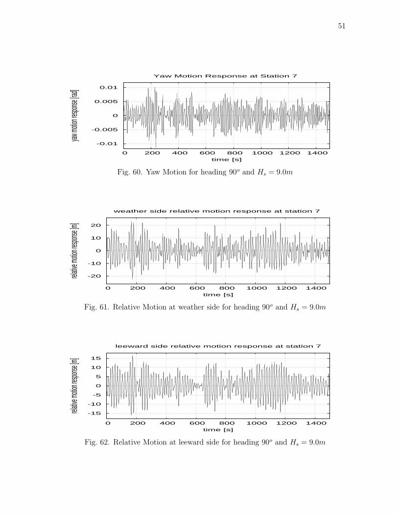
51
-0.01
-0.005
0
0.005
0.01
0 200 400 600 800 1000 1200 1400
yaw mo
tion res
ponse
[rad]
time [s]
Yaw Motion Response at Station 7
Fig. 60. Yaw Motion for heading 90o and Hs = 9.0m
-20
-10
0
10
20
0 200 400 600 800 1000 1200 1400
relative
motion
respon
se [m]
time [s]
weather side relative motion response at station 7
Fig. 61. Relative Motion at weather side for heading 90o and Hs = 9.0m
-15
-10
-5
0
5
10
15
0 200 400 600 800 1000 1200 1400
relative
motion
respon
se [m]
time [s]
leeward side relative motion response at station 7
Fig. 62. Relative Motion at leeward side for heading 90o and Hs = 9.0m
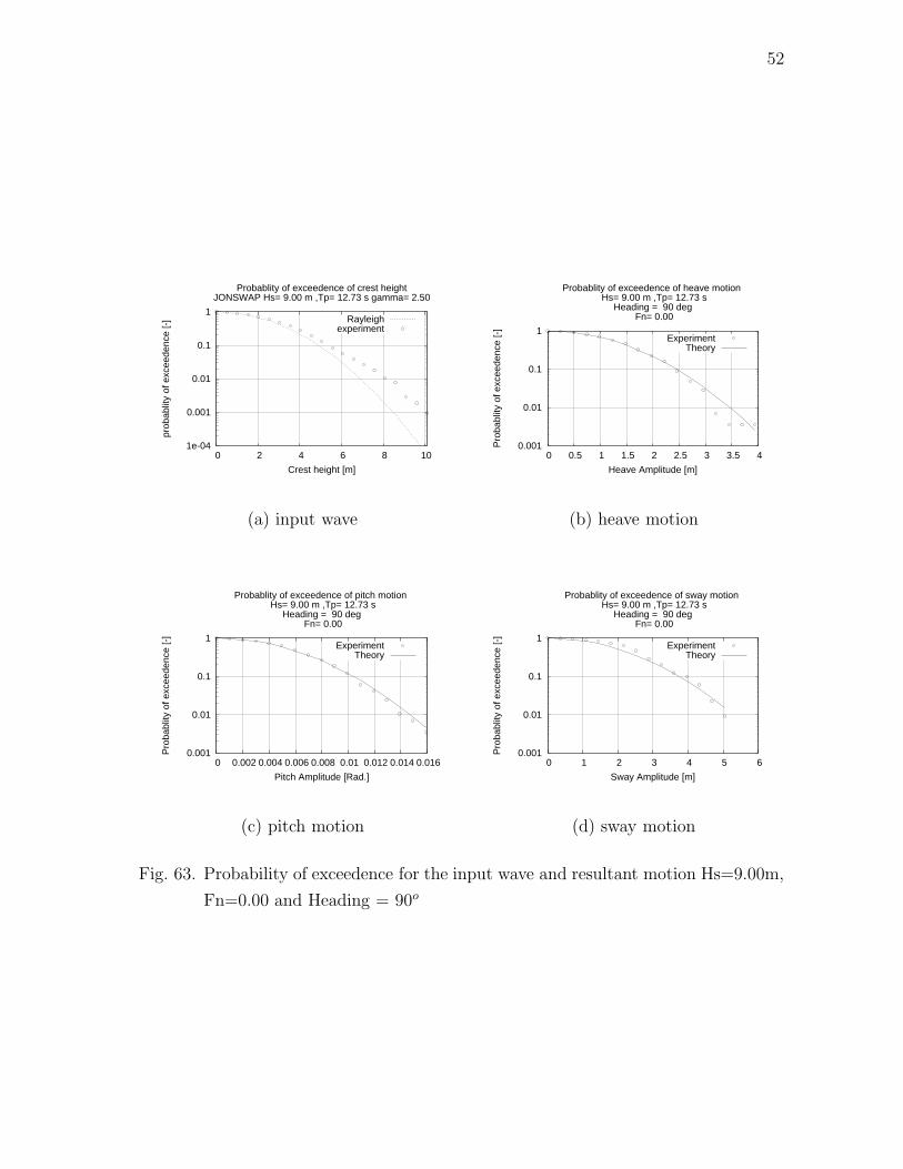
52
1e-04
0.001
0.01
0.1
1
0 2 4 6 8 10
prob
ablit
y of
exc
eede
nce
[-]
Crest height [m]
Probablity of exceedence of crest heightJONSWAP Hs= 9.00 m ,Tp= 12.73 s gamma= 2.50
Rayleighexperiment
(a) input wave
0.001
0.01
0.1
1
0 0.5 1 1.5 2 2.5 3 3.5 4
Pro
babl
ity o
f exc
eede
nce
[-]
Heave Amplitude [m]
Probablity of exceedence of heave motion Hs= 9.00 m ,Tp= 12.73 s
Heading = 90 deg Fn= 0.00
ExperimentTheory
(b) heave motion
0.001
0.01
0.1
1
0 0.002 0.004 0.006 0.008 0.01 0.012 0.014 0.016
Pro
babl
ity o
f exc
eede
nce
[-]
Pitch Amplitude [Rad.]
Probablity of exceedence of pitch motion Hs= 9.00 m ,Tp= 12.73 s
Heading = 90 deg Fn= 0.00
ExperimentTheory
(c) pitch motion
0.001
0.01
0.1
1
0 1 2 3 4 5 6
Pro
babl
ity o
f exc
eede
nce
[-]
Sway Amplitude [m]
Probablity of exceedence of sway motion Hs= 9.00 m ,Tp= 12.73 s
Heading = 90 deg Fn= 0.00
ExperimentTheory
(d) sway motion
Fig. 63. Probability of exceedence for the input wave and resultant motion Hs=9.00m,
Fn=0.00 and Heading = 90o
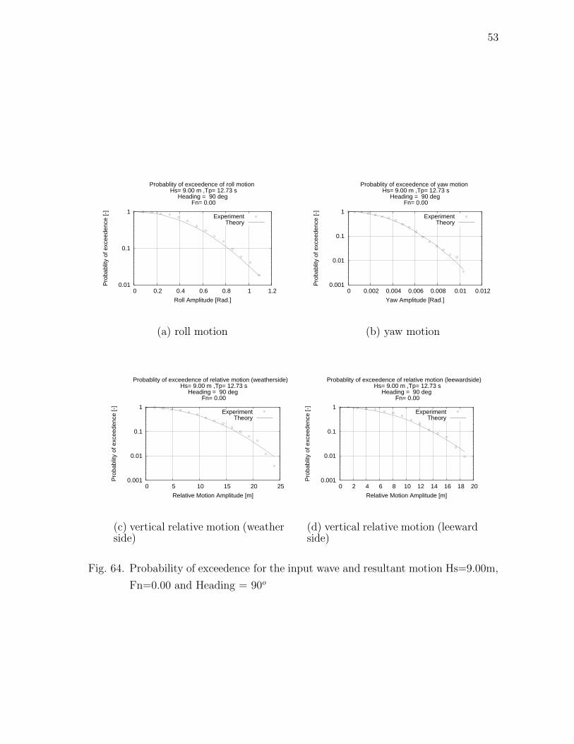
53
0.01
0.1
1
0 0.2 0.4 0.6 0.8 1 1.2
Pro
babl
ity o
f exc
eede
nce
[-]
Roll Amplitude [Rad.]
Probablity of exceedence of roll motion Hs= 9.00 m ,Tp= 12.73 s
Heading = 90 deg Fn= 0.00
ExperimentTheory
(a) roll motion
0.001
0.01
0.1
1
0 0.002 0.004 0.006 0.008 0.01 0.012
Pro
babl
ity o
f exc
eede
nce
[-]
Yaw Amplitude [Rad.]
Probablity of exceedence of yaw motion Hs= 9.00 m ,Tp= 12.73 s
Heading = 90 deg Fn= 0.00
ExperimentTheory
(b) yaw motion
0.001
0.01
0.1
1
0 5 10 15 20 25
Pro
babl
ity o
f exc
eede
nce
[-]
Relative Motion Amplitude [m]
Probablity of exceedence of relative motion (weatherside) Hs= 9.00 m ,Tp= 12.73 s
Heading = 90 deg Fn= 0.00
ExperimentTheory
(c) vertical relative motion (weatherside)
0.001
0.01
0.1
1
0 2 4 6 8 10 12 14 16 18 20
Pro
babl
ity o
f exc
eede
nce
[-]
Relative Motion Amplitude [m]
Probablity of exceedence of relative motion (leewardside) Hs= 9.00 m ,Tp= 12.73 s
Heading = 90 deg Fn= 0.00
ExperimentTheory
(d) vertical relative motion (leewardside)
Fig. 64. Probability of exceedence for the input wave and resultant motion Hs=9.00m,
Fn=0.00 and Heading = 90o
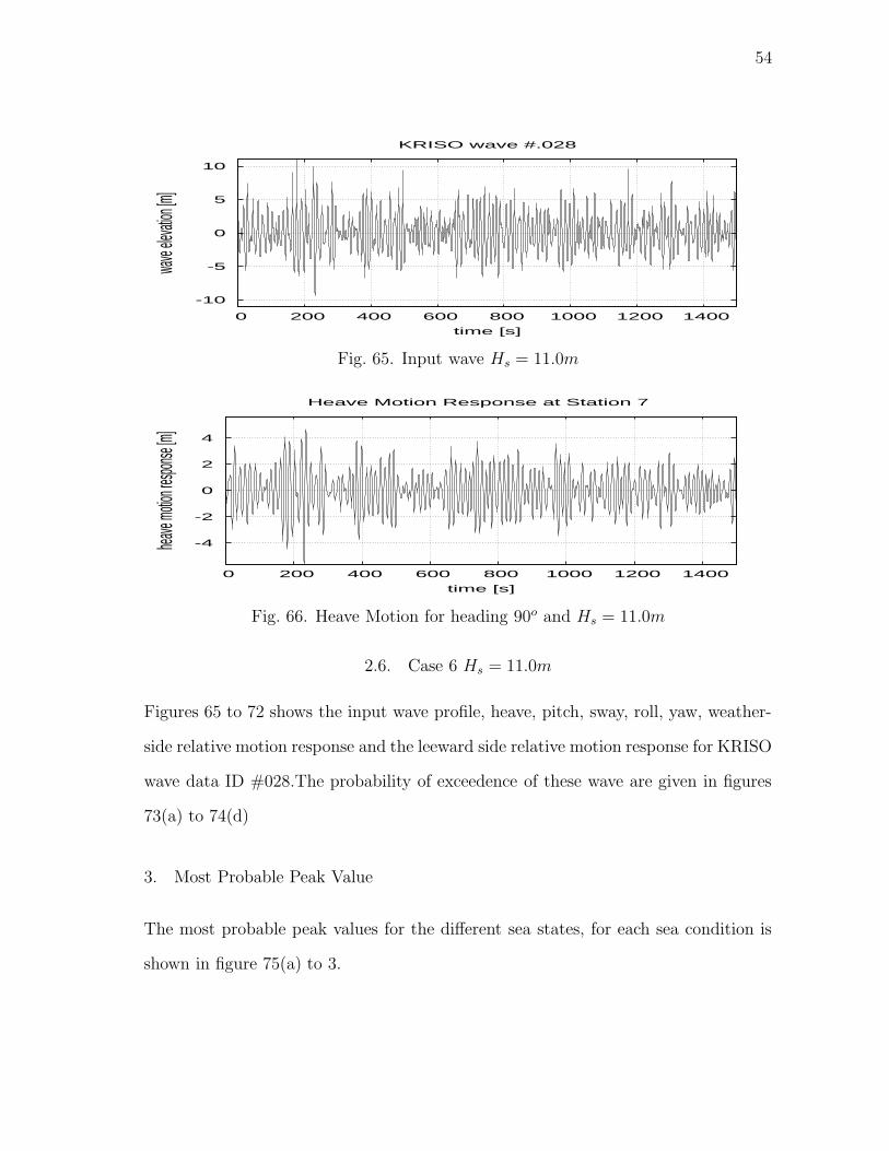
54
-10
-5
0
5
10
0 200 400 600 800 1000 1200 1400
wave
elevat
ion [m
]
time [s]
KRISO wave #.028
Fig. 65. Input wave Hs = 11.0m
-4
-2
0
2
4
0 200 400 600 800 1000 1200 1400
heave
motion
respon
se [m]
time [s]
Heave Motion Response at Station 7
Fig. 66. Heave Motion for heading 90o and Hs = 11.0m
2.6. Case 6 Hs = 11.0m
Figures 65 to 72 shows the input wave profile, heave, pitch, sway, roll, yaw, weather-
side relative motion response and the leeward side relative motion response for KRISO
wave data ID #028.The probability of exceedence of these wave are given in figures
73(a) to 74(d)
3. Most Probable Peak Value
The most probable peak values for the different sea states, for each sea condition is
shown in figure 75(a) to 3.

55
-0.02
-0.015
-0.01
-0.005
0
0.005
0.01
0.015
0.02
0 200 400 600 800 1000 1200 1400
pitch m
otion re
sponse
[rad]
time [s]
Pitch Motion Response at Station 7
Fig. 67. Pitch Motion for heading 90o and Hs = 11.0m
-6
-4
-2
0
2
4
6
0 200 400 600 800 1000 1200 1400
sway m
otion re
sponse
[m]
time [s]
Sway Motion Response at Station 7
Fig. 68. Sway Motion for heading 90o and Hs = 11.0m
-1.5
-1
-0.5
0
0.5
1
1.5
0 200 400 600 800 1000 1200 1400
roll mo
tion res
ponse
[rad]
time [s]
Roll Motion Response at Station 7
Fig. 69. Roll Motion for heading 90o and Hs = 11.0m
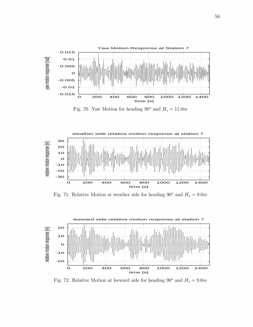
56
-0.015
-0.01
-0.005
0
0.005
0.01
0.015
0 200 400 600 800 1000 1200 1400
yaw mo
tion res
ponse
[rad]
time [s]
Yaw Motion Response at Station 7
Fig. 70. Yaw Motion for heading 90o and Hs = 11.0m
-30
-20
-10
0
10
20
30
0 200 400 600 800 1000 1200 1400
relative
motion
respon
se [m]
time [s]
weather side relative motion response at station 7
Fig. 71. Relative Motion at weather side for heading 90o and Hs = 9.0m
-20
-10
0
10
20
0 200 400 600 800 1000 1200 1400
relative
motion
respon
se [m]
time [s]
leeward side relative motion response at station 7
Fig. 72. Relative Motion at leeward side for heading 90o and Hs = 9.0m

57
1e-04
0.001
0.01
0.1
1
0 2 4 6 8 10 12
prob
ablit
y of
exc
eede
nce
[-]
Crest height [m]
Probablity of exceedence of crest heightJONSWAP Hs=11.00 m ,Tp= 13.37 s gamma= 2.50
Rayleighexperiment
(a) input wave
0.001
0.01
0.1
1
0 0.5 1 1.5 2 2.5 3 3.5 4 4.5
Pro
babl
ity o
f exc
eede
nce
[-]
Heave Amplitude [m]
Probablity of exceedence of heave motion Hs=11.00 m ,Tp= 13.37 s
Heading = 90 deg Fn= 0.00
ExperimentTheory
(b) heave
0.01
0.1
1
0 0.002 0.004 0.006 0.008 0.01 0.012 0.014 0.016 0.018 0.02
Pro
babl
ity o
f exc
eede
nce
[-]
Pitch Amplitude [Rad.]
Probablity of exceedence of pitch motion Hs=11.00 m ,Tp= 13.37 s
Heading = 90 deg Fn= 0.00
ExperimentTheory
(c) pitch
0.001
0.01
0.1
1
0 1 2 3 4 5 6 7 8 9
Pro
babl
ity o
f exc
eede
nce
[-]
Sway Amplitude [m]
Probablity of exceedence of sway motion Hs=11.00 m ,Tp= 13.37 s
Heading = 90 deg Fn= 0.00
ExperimentTheory
(d) sway
Fig. 73. Probability of exceedence for the input wave and resultant motion Hs=11.00m,
Fn=0.00 and Heading = 90o
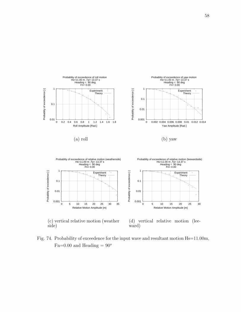
58
0.01
0.1
1
0 0.2 0.4 0.6 0.8 1 1.2 1.4 1.6 1.8
Pro
babl
ity o
f exc
eede
nce
[-]
Roll Amplitude [Rad.]
Probablity of exceedence of roll motion Hs=11.00 m ,Tp= 13.37 s
Heading = 90 deg Fn= 0.00
ExperimentTheory
(a) roll
0.001
0.01
0.1
1
0 0.002 0.004 0.006 0.008 0.01 0.012 0.014
Pro
babl
ity o
f exc
eede
nce
[-]
Yaw Amplitude [Rad.]
Probablity of exceedence of yaw motion Hs=11.00 m ,Tp= 13.37 s
Heading = 90 deg Fn= 0.00
ExperimentTheory
(b) yaw
0.001
0.01
0.1
1
0 5 10 15 20 25 30 35
Pro
babl
ity o
f exc
eede
nce
[-]
Relative Motion Amplitude [m]
Probablity of exceedence of relative motion (weatherside) Hs=11.00 m ,Tp= 13.37 s
Heading = 90 deg Fn= 0.00
ExperimentTheory
(c) vertical relative motion (weatherside)
0.001
0.01
0.1
1
0 5 10 15 20 25 30
Pro
babl
ity o
f exc
eede
nce
[-]
Relative Motion Amplitude [m]
Probablity of exceedence of relative motion (leewardside) Hs=11.00 m ,Tp= 13.37 s
Heading = 90 deg Fn= 0.00
ExperimentTheory
(d) vertical relative motion (lee-ward)
Fig. 74. Probability of exceedence for the input wave and resultant motion Hs=11.00m,
Fn=0.00 and Heading = 90o
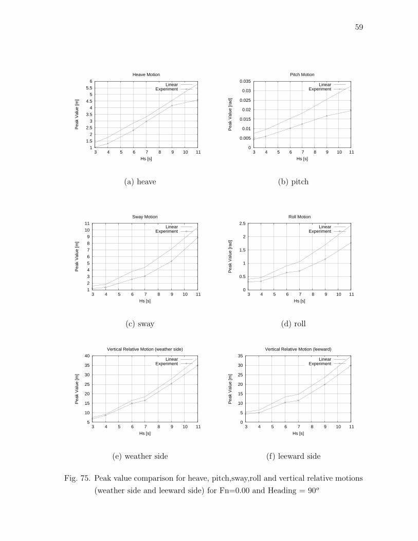
59
1
1.5
2
2.5
3
3.5
4
4.5
5
5.5
6
3 4 5 6 7 8 9 10 11
Pea
k V
alue
[m]
Hs [s]
Heave Motion
LinearExperiment
(a) heave
0
0.005
0.01
0.015
0.02
0.025
0.03
0.035
3 4 5 6 7 8 9 10 11
Pea
k V
alue
[rad
]
Hs [s]
Pitch Motion
LinearExperiment
(b) pitch
1
2
3
4
5
6
7
8
9
10
11
3 4 5 6 7 8 9 10 11
Pea
k V
alue
[m]
Hs [s]
Sway Motion
LinearExperiment
(c) sway
0
0.5
1
1.5
2
2.5
3 4 5 6 7 8 9 10 11
Pea
k V
alue
[rad
]
Hs [s]
Roll Motion
LinearExperiment
(d) roll
5
10
15
20
25
30
35
40
3 4 5 6 7 8 9 10 11
Pea
k V
alue
[m]
Hs [s]
Vertical Relative Motion (weather side)
LinearExperiment
(e) weather side
0
5
10
15
20
25
30
35
3 4 5 6 7 8 9 10 11
Pea
k V
alue
[m]
Hs [s]
Vertical Relative Motion (leeward)
LinearExperiment
(f) leeward side
Fig. 75. Peak value comparison for heave, pitch,sway,roll and vertical relative motions
(weather side and leeward side) for Fn=0.00 and Heading = 90o
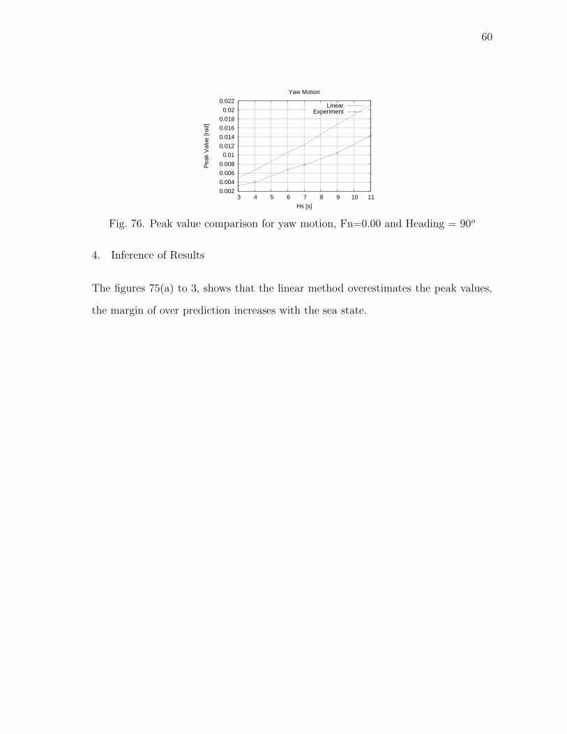
60
0.002
0.004
0.006
0.008
0.01
0.012
0.014
0.016
0.018
0.02
0.022
3 4 5 6 7 8 9 10 11
Pea
k V
alue
[rad
]Hs [s]
Yaw Motion
LinearExperiment
Fig. 76. Peak value comparison for yaw motion, Fn=0.00 and Heading = 90o
4. Inference of Results
The figures 75(a) to 3, shows that the linear method overestimates the peak values,
the margin of over prediction increases with the sea state.
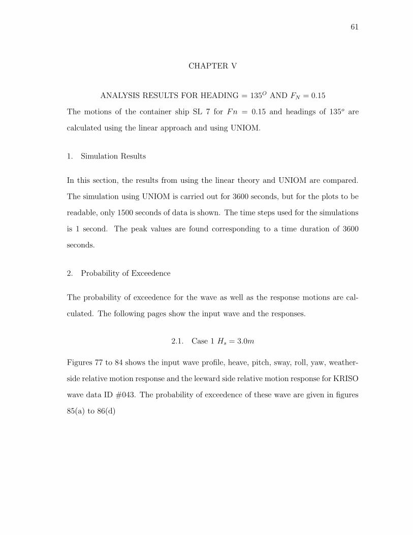
61
CHAPTER V
ANALYSIS RESULTS FOR HEADING = 135O AND FN = 0.15
The motions of the container ship SL 7 for Fn = 0.15 and headings of 135o are
calculated using the linear approach and using UNIOM.
1. Simulation Results
In this section, the results from using the linear theory and UNIOM are compared.
The simulation using UNIOM is carried out for 3600 seconds, but for the plots to be
readable, only 1500 seconds of data is shown. The time steps used for the simulations
is 1 second. The peak values are found corresponding to a time duration of 3600
seconds.
2. Probability of Exceedence
The probability of exceedence for the wave as well as the response motions are cal-
culated. The following pages show the input wave and the responses.
2.1. Case 1 Hs = 3.0m
Figures 77 to 84 shows the input wave profile, heave, pitch, sway, roll, yaw, weather-
side relative motion response and the leeward side relative motion response for KRISO
wave data ID #043. The probability of exceedence of these wave are given in figures
85(a) to 86(d)
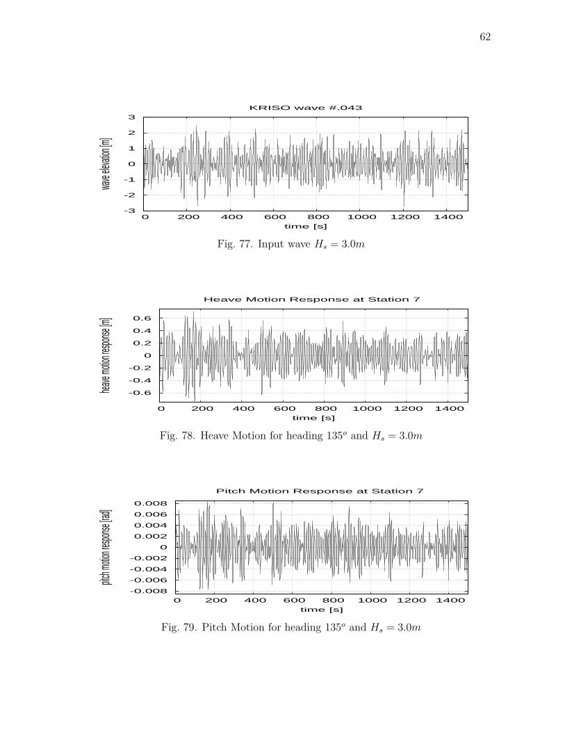
62
-3
-2
-1
0
1
2
3
0 200 400 600 800 1000 1200 1400
wave
elevat
ion [m
]
time [s]
KRISO wave #.043
Fig. 77. Input wave Hs = 3.0m
-0.6
-0.4
-0.2
0
0.2
0.4
0.6
0 200 400 600 800 1000 1200 1400
heave
motion
respon
se [m]
time [s]
Heave Motion Response at Station 7
Fig. 78. Heave Motion for heading 135o and Hs = 3.0m
-0.008
-0.006
-0.004
-0.002
0
0.002
0.004
0.006
0.008
0 200 400 600 800 1000 1200 1400
pitch m
otion re
sponse
[rad]
time [s]
Pitch Motion Response at Station 7
Fig. 79. Pitch Motion for heading 135o and Hs = 3.0m
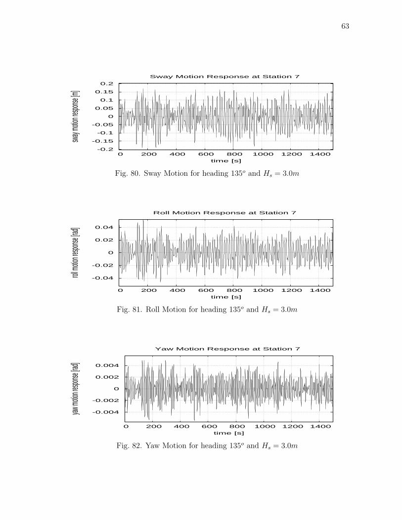
63
-0.2
-0.15
-0.1
-0.05
0
0.05
0.1
0.15
0.2
0 200 400 600 800 1000 1200 1400
sway m
otion re
sponse
[m]
time [s]
Sway Motion Response at Station 7
Fig. 80. Sway Motion for heading 135o and Hs = 3.0m
-0.04
-0.02
0
0.02
0.04
0 200 400 600 800 1000 1200 1400
roll mo
tion res
ponse
[rad]
time [s]
Roll Motion Response at Station 7
Fig. 81. Roll Motion for heading 135o and Hs = 3.0m
-0.004
-0.002
0
0.002
0.004
0 200 400 600 800 1000 1200 1400
yaw mo
tion res
ponse
[rad]
time [s]
Yaw Motion Response at Station 7
Fig. 82. Yaw Motion for heading 135o and Hs = 3.0m
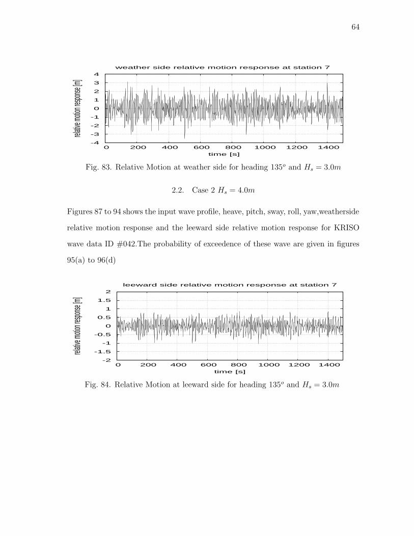
64
-4
-3
-2
-1
0
1
2
3
4
0 200 400 600 800 1000 1200 1400
relative
motion
respon
se [m]
time [s]
weather side relative motion response at station 7
Fig. 83. Relative Motion at weather side for heading 135o and Hs = 3.0m
2.2. Case 2 Hs = 4.0m
Figures 87 to 94 shows the input wave profile, heave, pitch, sway, roll, yaw,weatherside
relative motion response and the leeward side relative motion response for KRISO
wave data ID #042.The probability of exceedence of these wave are given in figures
95(a) to 96(d)
-2
-1.5
-1
-0.5
0
0.5
1
1.5
2
0 200 400 600 800 1000 1200 1400
relative
motion
respon
se [m]
time [s]
leeward side relative motion response at station 7
Fig. 84. Relative Motion at leeward side for heading 135o and Hs = 3.0m
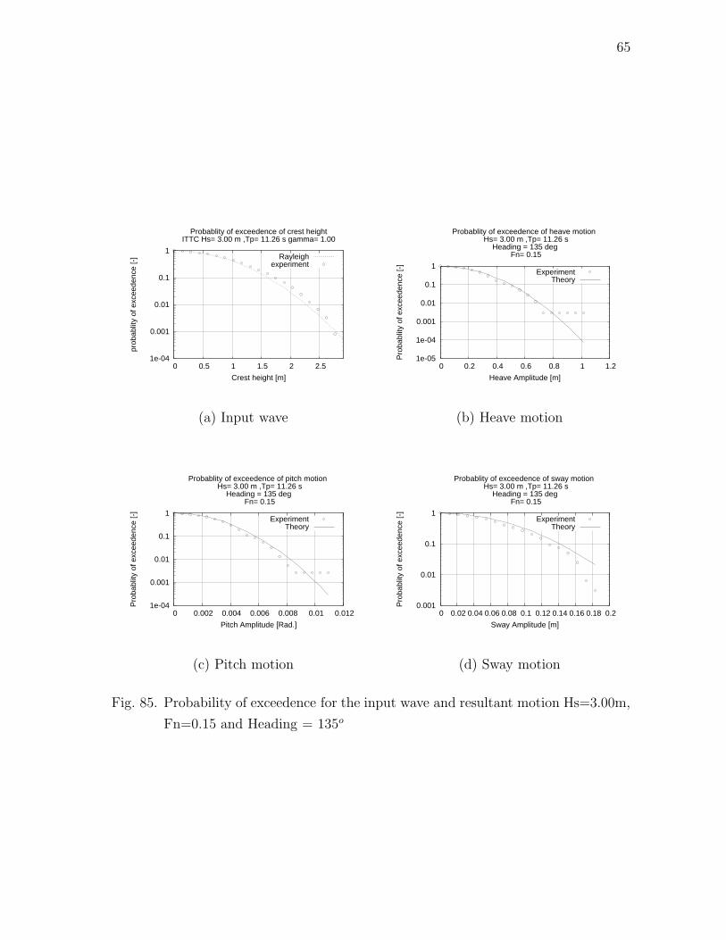
65
1e-04
0.001
0.01
0.1
1
0 0.5 1 1.5 2 2.5
prob
ablit
y of
exc
eede
nce
[-]
Crest height [m]
Probablity of exceedence of crest heightITTC Hs= 3.00 m ,Tp= 11.26 s gamma= 1.00
Rayleighexperiment
(a) Input wave
1e-05
1e-04
0.001
0.01
0.1
1
0 0.2 0.4 0.6 0.8 1 1.2
Pro
babl
ity o
f exc
eede
nce
[-]
Heave Amplitude [m]
Probablity of exceedence of heave motion Hs= 3.00 m ,Tp= 11.26 s
Heading = 135 deg Fn= 0.15
ExperimentTheory
(b) Heave motion
1e-04
0.001
0.01
0.1
1
0 0.002 0.004 0.006 0.008 0.01 0.012
Pro
babl
ity o
f exc
eede
nce
[-]
Pitch Amplitude [Rad.]
Probablity of exceedence of pitch motion Hs= 3.00 m ,Tp= 11.26 s
Heading = 135 deg Fn= 0.15
ExperimentTheory
(c) Pitch motion
0.001
0.01
0.1
1
0 0.02 0.04 0.06 0.08 0.1 0.12 0.14 0.16 0.18 0.2
Pro
babl
ity o
f exc
eede
nce
[-]
Sway Amplitude [m]
Probablity of exceedence of sway motion Hs= 3.00 m ,Tp= 11.26 s
Heading = 135 deg Fn= 0.15
ExperimentTheory
(d) Sway motion
Fig. 85. Probability of exceedence for the input wave and resultant motion Hs=3.00m,
Fn=0.15 and Heading = 135o
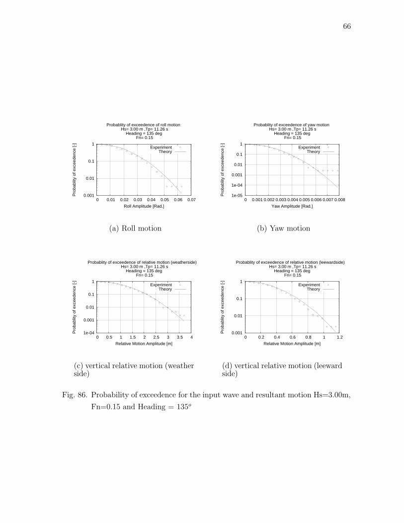
66
0.001
0.01
0.1
1
0 0.01 0.02 0.03 0.04 0.05 0.06 0.07
Pro
babl
ity o
f exc
eede
nce
[-]
Roll Amplitude [Rad.]
Probablity of exceedence of roll motion Hs= 3.00 m ,Tp= 11.26 s
Heading = 135 deg Fn= 0.15
ExperimentTheory
(a) Roll motion
1e-05
1e-04
0.001
0.01
0.1
1
0 0.001 0.002 0.003 0.004 0.005 0.006 0.007 0.008
Pro
babl
ity o
f exc
eede
nce
[-]
Yaw Amplitude [Rad.]
Probablity of exceedence of yaw motion Hs= 3.00 m ,Tp= 11.26 s
Heading = 135 deg Fn= 0.15
ExperimentTheory
(b) Yaw motion
1e-04
0.001
0.01
0.1
1
0 0.5 1 1.5 2 2.5 3 3.5 4
Pro
babl
ity o
f exc
eede
nce
[-]
Relative Motion Amplitude [m]
Probablity of exceedence of relative motion (weatherside) Hs= 3.00 m ,Tp= 11.26 s
Heading = 135 deg Fn= 0.15
ExperimentTheory
(c) vertical relative motion (weatherside)
0.001
0.01
0.1
1
0 0.2 0.4 0.6 0.8 1 1.2
Pro
babl
ity o
f exc
eede
nce
[-]
Relative Motion Amplitude [m]
Probablity of exceedence of relative motion (leewardside) Hs= 3.00 m ,Tp= 11.26 s
Heading = 135 deg Fn= 0.15
ExperimentTheory
(d) vertical relative motion (leewardside)
Fig. 86. Probability of exceedence for the input wave and resultant motion Hs=3.00m,
Fn=0.15 and Heading = 135o
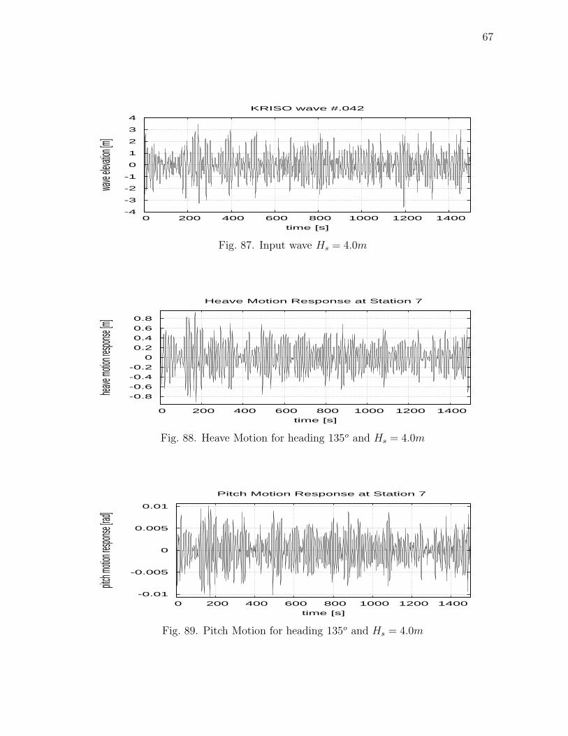
67
-4
-3
-2
-1
0
1
2
3
4
0 200 400 600 800 1000 1200 1400
wave
elevat
ion [m
]
time [s]
KRISO wave #.042
Fig. 87. Input wave Hs = 4.0m
-0.8
-0.6
-0.4
-0.2
0
0.2
0.4
0.6
0.8
0 200 400 600 800 1000 1200 1400
heave
motion
respon
se [m]
time [s]
Heave Motion Response at Station 7
Fig. 88. Heave Motion for heading 135o and Hs = 4.0m
-0.01
-0.005
0
0.005
0.01
0 200 400 600 800 1000 1200 1400
pitch m
otion re
sponse
[rad]
time [s]
Pitch Motion Response at Station 7
Fig. 89. Pitch Motion for heading 135o and Hs = 4.0m
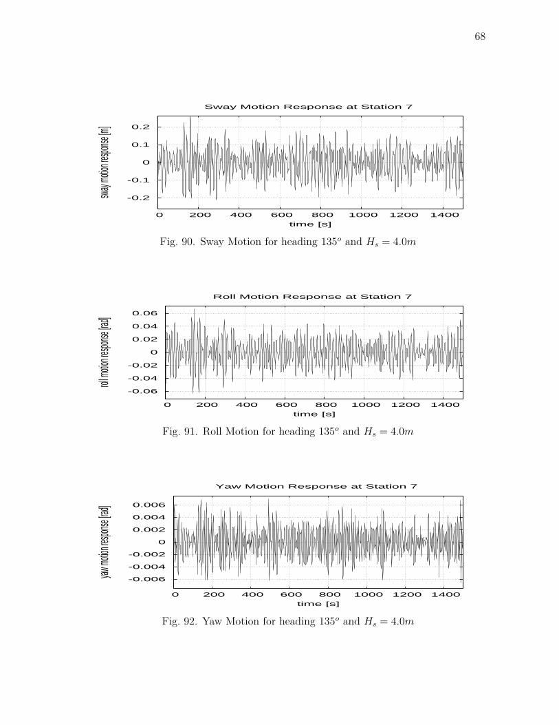
68
-0.2
-0.1
0
0.1
0.2
0 200 400 600 800 1000 1200 1400
sway m
otion re
sponse
[m]
time [s]
Sway Motion Response at Station 7
Fig. 90. Sway Motion for heading 135o and Hs = 4.0m
-0.06
-0.04
-0.02
0
0.02
0.04
0.06
0 200 400 600 800 1000 1200 1400
roll mo
tion res
ponse
[rad]
time [s]
Roll Motion Response at Station 7
Fig. 91. Roll Motion for heading 135o and Hs = 4.0m
-0.006
-0.004
-0.002
0
0.002
0.004
0.006
0 200 400 600 800 1000 1200 1400
yaw mo
tion res
ponse
[rad]
time [s]
Yaw Motion Response at Station 7
Fig. 92. Yaw Motion for heading 135o and Hs = 4.0m
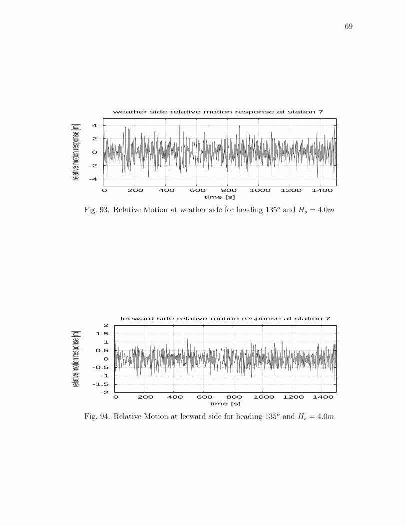
69
-4
-2
0
2
4
0 200 400 600 800 1000 1200 1400
relative
motion
respon
se [m]
time [s]
weather side relative motion response at station 7
Fig. 93. Relative Motion at weather side for heading 135o and Hs = 4.0m
-2
-1.5
-1
-0.5
0
0.5
1
1.5
2
0 200 400 600 800 1000 1200 1400
relative
motion
respon
se [m]
time [s]
leeward side relative motion response at station 7
Fig. 94. Relative Motion at leeward side for heading 135o and Hs = 4.0m

70
1e-04
0.001
0.01
0.1
1
0 0.5 1 1.5 2 2.5 3 3.5 4
prob
ablit
y of
exc
eede
nce
[-]
Crest height [m]
Probablity of exceedence of crest heightITTC Hs= 4.00 m ,Tp= 11.26 s gamma= 1.00
Rayleighexperiment
(a) input wave
1e-04
0.001
0.01
0.1
1
0 0.2 0.4 0.6 0.8 1 1.2
Pro
babl
ity o
f exc
eede
nce
[-]
Heave Amplitude [m]
Probablity of exceedence of heave motion Hs= 4.00 m ,Tp= 11.26 s
Heading = 135 deg Fn= 0.15
ExperimentTheory
(b) heave motion
0.001
0.01
0.1
1
0 0.002 0.004 0.006 0.008 0.01 0.012
Pro
babl
ity o
f exc
eede
nce
[-]
Pitch Amplitude [Rad.]
Probablity of exceedence of pitch motion Hs= 4.00 m ,Tp= 11.26 s
Heading = 135 deg Fn= 0.15
ExperimentTheory
(c) pitch motion
1e-04
0.001
0.01
0.1
1
0 0.05 0.1 0.15 0.2 0.25 0.3
Pro
babl
ity o
f exc
eede
nce
[-]
Sway Amplitude [m]
Probablity of exceedence of sway motion Hs= 4.00 m ,Tp= 11.26 s
Heading = 135 deg Fn= 0.15
ExperimentTheory
(d) sway motion
Fig. 95. Probability of exceedence for the input wave and resultant motion Hs=4.00m,
Fn=0.15 and Heading = 135o
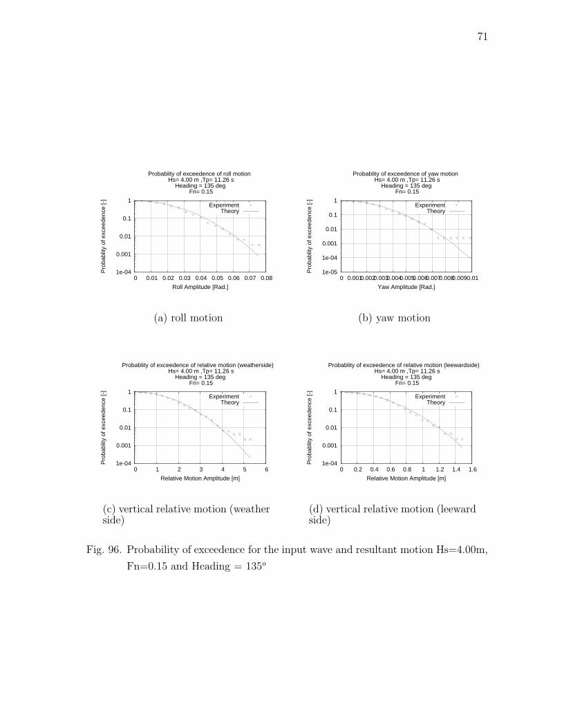
71
1e-04
0.001
0.01
0.1
1
0 0.01 0.02 0.03 0.04 0.05 0.06 0.07 0.08
Pro
babl
ity o
f exc
eede
nce
[-]
Roll Amplitude [Rad.]
Probablity of exceedence of roll motion Hs= 4.00 m ,Tp= 11.26 s
Heading = 135 deg Fn= 0.15
ExperimentTheory
(a) roll motion
1e-05
1e-04
0.001
0.01
0.1
1
0 0.001 0.002 0.003 0.004 0.005 0.006 0.007 0.008 0.009 0.01
Pro
babl
ity o
f exc
eede
nce
[-]
Yaw Amplitude [Rad.]
Probablity of exceedence of yaw motion Hs= 4.00 m ,Tp= 11.26 s
Heading = 135 deg Fn= 0.15
ExperimentTheory
(b) yaw motion
1e-04
0.001
0.01
0.1
1
0 1 2 3 4 5 6
Pro
babl
ity o
f exc
eede
nce
[-]
Relative Motion Amplitude [m]
Probablity of exceedence of relative motion (weatherside) Hs= 4.00 m ,Tp= 11.26 s
Heading = 135 deg Fn= 0.15
ExperimentTheory
(c) vertical relative motion (weatherside)
1e-04
0.001
0.01
0.1
1
0 0.2 0.4 0.6 0.8 1 1.2 1.4 1.6
Pro
babl
ity o
f exc
eede
nce
[-]
Relative Motion Amplitude [m]
Probablity of exceedence of relative motion (leewardside) Hs= 4.00 m ,Tp= 11.26 s
Heading = 135 deg Fn= 0.15
ExperimentTheory
(d) vertical relative motion (leewardside)
Fig. 96. Probability of exceedence for the input wave and resultant motion Hs=4.00m,
Fn=0.15 and Heading = 135o
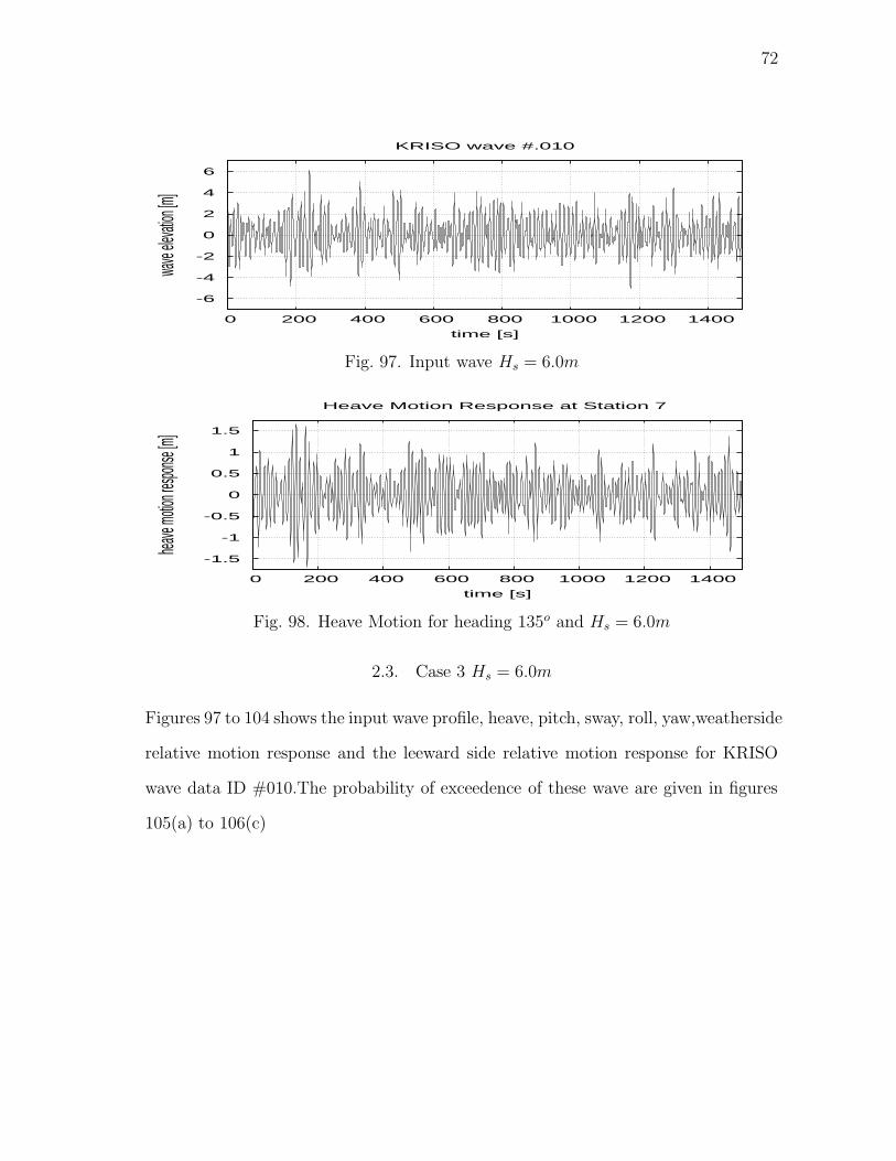
72
-6
-4
-2
0
2
4
6
0 200 400 600 800 1000 1200 1400
wave
elevat
ion [m
]
time [s]
KRISO wave #.010
Fig. 97. Input wave Hs = 6.0m
-1.5
-1
-0.5
0
0.5
1
1.5
0 200 400 600 800 1000 1200 1400
heave
motion
respon
se [m]
time [s]
Heave Motion Response at Station 7
Fig. 98. Heave Motion for heading 135o and Hs = 6.0m
2.3. Case 3 Hs = 6.0m
Figures 97 to 104 shows the input wave profile, heave, pitch, sway, roll, yaw,weatherside
relative motion response and the leeward side relative motion response for KRISO
wave data ID #010.The probability of exceedence of these wave are given in figures
105(a) to 106(c)
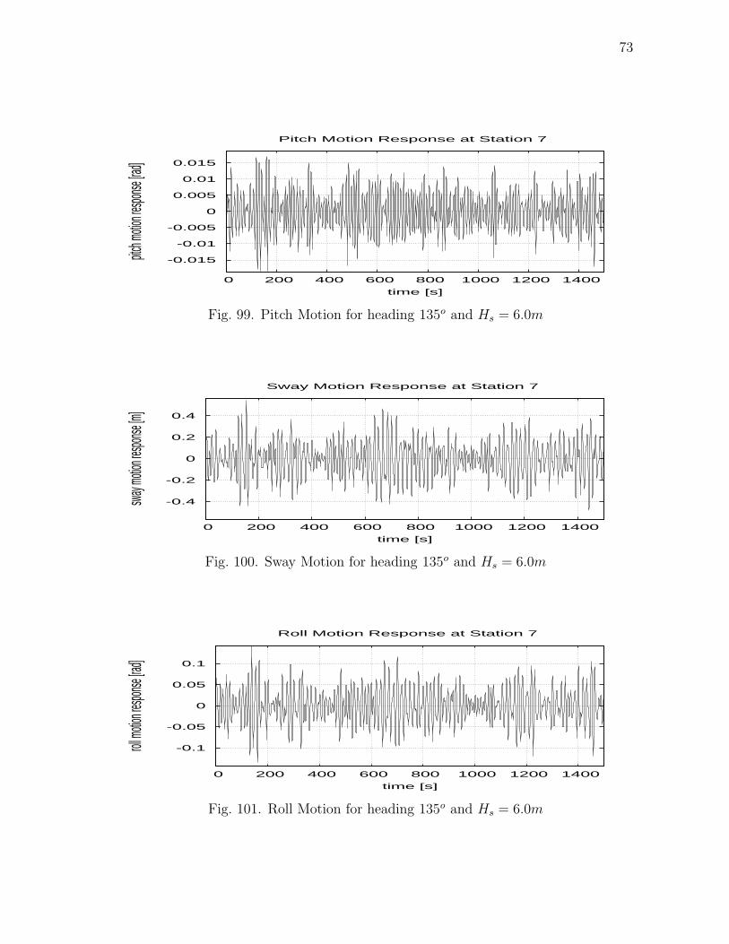
73
-0.015
-0.01
-0.005
0
0.005
0.01
0.015
0 200 400 600 800 1000 1200 1400
pitch m
otion re
sponse
[rad]
time [s]
Pitch Motion Response at Station 7
Fig. 99. Pitch Motion for heading 135o and Hs = 6.0m
-0.4
-0.2
0
0.2
0.4
0 200 400 600 800 1000 1200 1400
sway m
otion re
sponse
[m]
time [s]
Sway Motion Response at Station 7
Fig. 100. Sway Motion for heading 135o and Hs = 6.0m
-0.1
-0.05
0
0.05
0.1
0 200 400 600 800 1000 1200 1400
roll mo
tion res
ponse
[rad]
time [s]
Roll Motion Response at Station 7
Fig. 101. Roll Motion for heading 135o and Hs = 6.0m
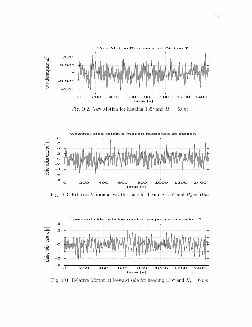
74
-0.01
-0.005
0
0.005
0.01
0 200 400 600 800 1000 1200 1400
yaw mo
tion res
ponse
[rad]
time [s]
Yaw Motion Response at Station 7
Fig. 102. Yaw Motion for heading 135o and Hs = 6.0m
-8
-6
-4
-2
0
2
4
6
8
0 200 400 600 800 1000 1200 1400
relative
motion
respon
se [m]
time [s]
weather side relative motion response at station 7
Fig. 103. Relative Motion at weather side for heading 135o and Hs = 6.0m
-3
-2
-1
0
1
2
3
0 200 400 600 800 1000 1200 1400
relative
motion
respon
se [m]
time [s]
leeward side relative motion response at station 7
Fig. 104. Relative Motion at leeward side for heading 135o and Hs = 6.0m
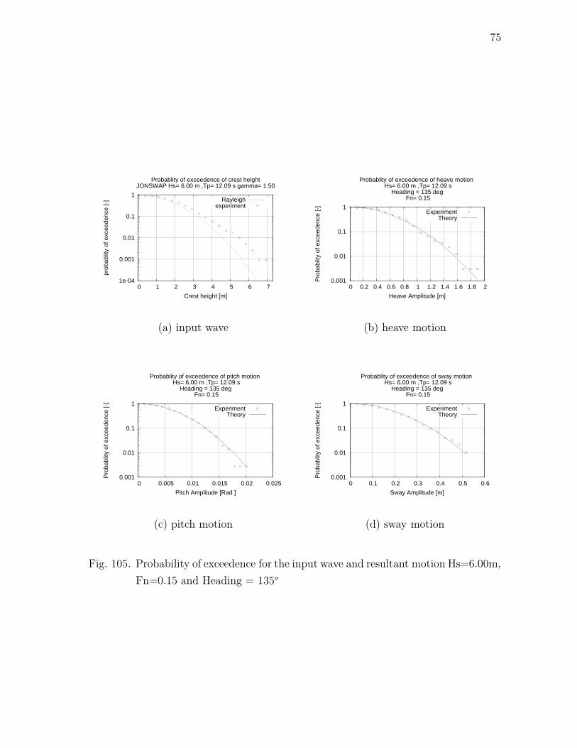
75
1e-04
0.001
0.01
0.1
1
0 1 2 3 4 5 6 7
prob
ablit
y of
exc
eede
nce
[-]
Crest height [m]
Probablity of exceedence of crest heightJONSWAP Hs= 6.00 m ,Tp= 12.09 s gamma= 1.50
Rayleighexperiment
(a) input wave
0.001
0.01
0.1
1
0 0.2 0.4 0.6 0.8 1 1.2 1.4 1.6 1.8 2
Pro
babl
ity o
f exc
eede
nce
[-]
Heave Amplitude [m]
Probablity of exceedence of heave motion Hs= 6.00 m ,Tp= 12.09 s
Heading = 135 deg Fn= 0.15
ExperimentTheory
(b) heave motion
0.001
0.01
0.1
1
0 0.005 0.01 0.015 0.02 0.025
Pro
babl
ity o
f exc
eede
nce
[-]
Pitch Amplitude [Rad.]
Probablity of exceedence of pitch motion Hs= 6.00 m ,Tp= 12.09 s
Heading = 135 deg Fn= 0.15
ExperimentTheory
(c) pitch motion
0.001
0.01
0.1
1
0 0.1 0.2 0.3 0.4 0.5 0.6
Pro
babl
ity o
f exc
eede
nce
[-]
Sway Amplitude [m]
Probablity of exceedence of sway motion Hs= 6.00 m ,Tp= 12.09 s
Heading = 135 deg Fn= 0.15
ExperimentTheory
(d) sway motion
Fig. 105. Probability of exceedence for the input wave and resultant motion Hs=6.00m,
Fn=0.15 and Heading = 135o
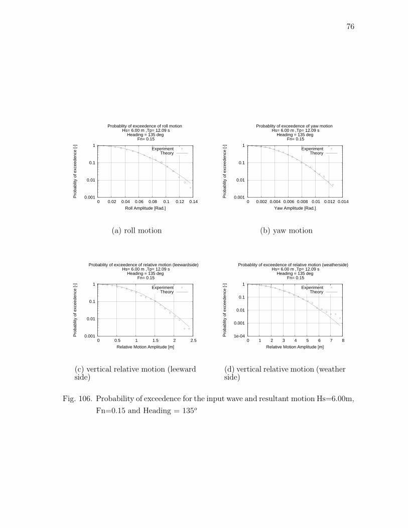
76
0.001
0.01
0.1
1
0 0.02 0.04 0.06 0.08 0.1 0.12 0.14
Pro
babl
ity o
f exc
eede
nce
[-]
Roll Amplitude [Rad.]
Probablity of exceedence of roll motion Hs= 6.00 m ,Tp= 12.09 s
Heading = 135 deg Fn= 0.15
ExperimentTheory
(a) roll motion
0.001
0.01
0.1
1
0 0.002 0.004 0.006 0.008 0.01 0.012 0.014
Pro
babl
ity o
f exc
eede
nce
[-]
Yaw Amplitude [Rad.]
Probablity of exceedence of yaw motion Hs= 6.00 m ,Tp= 12.09 s
Heading = 135 deg Fn= 0.15
ExperimentTheory
(b) yaw motion
0.001
0.01
0.1
1
0 0.5 1 1.5 2 2.5
Pro
babl
ity o
f exc
eede
nce
[-]
Relative Motion Amplitude [m]
Probablity of exceedence of relative motion (leewardside) Hs= 6.00 m ,Tp= 12.09 s
Heading = 135 deg Fn= 0.15
ExperimentTheory
(c) vertical relative motion (leewardside)
1e-04
0.001
0.01
0.1
1
0 1 2 3 4 5 6 7 8
Pro
babl
ity o
f exc
eede
nce
[-]
Relative Motion Amplitude [m]
Probablity of exceedence of relative motion (weatherside) Hs= 6.00 m ,Tp= 12.09 s
Heading = 135 deg Fn= 0.15
ExperimentTheory
(d) vertical relative motion (weatherside)
Fig. 106. Probability of exceedence for the input wave and resultant motion Hs=6.00m,
Fn=0.15 and Heading = 135o
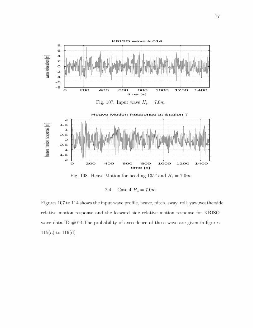
77
-8
-6
-4
-2
0
2
4
6
8
0 200 400 600 800 1000 1200 1400
wave
elevat
ion [m
]
time [s]
KRISO wave #.014
Fig. 107. Input wave Hs = 7.0m
-2
-1.5
-1
-0.5
0
0.5
1
1.5
2
0 200 400 600 800 1000 1200 1400
heave
motion
respon
se [m]
time [s]
Heave Motion Response at Station 7
Fig. 108. Heave Motion for heading 135o and Hs = 7.0m
2.4. Case 4 Hs = 7.0m
Figures 107 to 114 shows the input wave profile, heave, pitch, sway, roll, yaw,weatherside
relative motion response and the leeward side relative motion response for KRISO
wave data ID #014.The probability of exceedence of these wave are given in figures
115(a) to 116(d)
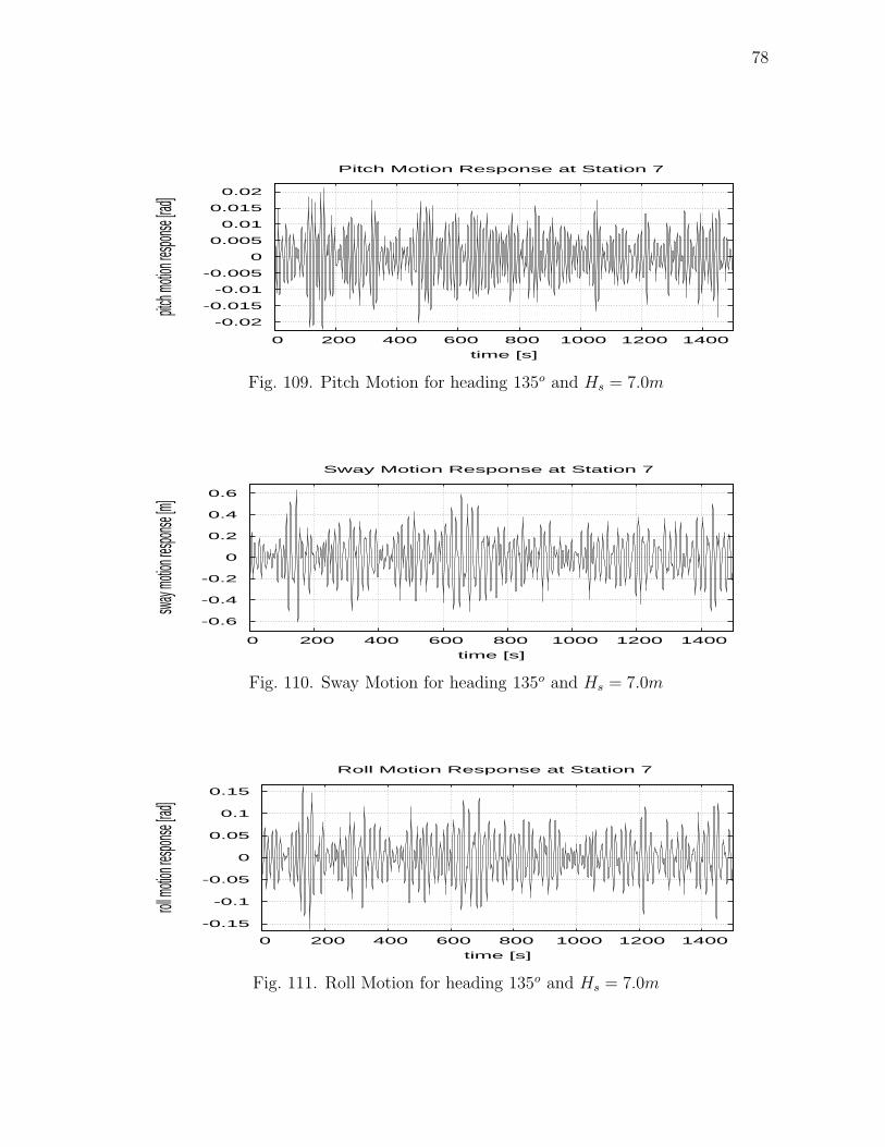
78
-0.02
-0.015
-0.01
-0.005
0
0.005
0.01
0.015
0.02
0 200 400 600 800 1000 1200 1400
pitch m
otion re
sponse
[rad]
time [s]
Pitch Motion Response at Station 7
Fig. 109. Pitch Motion for heading 135o and Hs = 7.0m
-0.6
-0.4
-0.2
0
0.2
0.4
0.6
0 200 400 600 800 1000 1200 1400
sway m
otion re
sponse
[m]
time [s]
Sway Motion Response at Station 7
Fig. 110. Sway Motion for heading 135o and Hs = 7.0m
-0.15
-0.1
-0.05
0
0.05
0.1
0.15
0 200 400 600 800 1000 1200 1400
roll mo
tion res
ponse
[rad]
time [s]
Roll Motion Response at Station 7
Fig. 111. Roll Motion for heading 135o and Hs = 7.0m
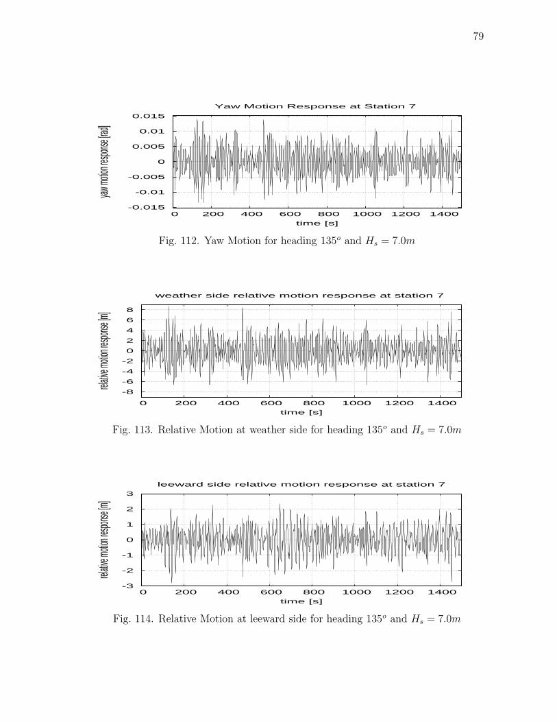
79
-0.015
-0.01
-0.005
0
0.005
0.01
0.015
0 200 400 600 800 1000 1200 1400
yaw mo
tion res
ponse
[rad]
time [s]
Yaw Motion Response at Station 7
Fig. 112. Yaw Motion for heading 135o and Hs = 7.0m
-8
-6
-4
-2
0
2
4
6
8
0 200 400 600 800 1000 1200 1400
relative
motion
respon
se [m]
time [s]
weather side relative motion response at station 7
Fig. 113. Relative Motion at weather side for heading 135o and Hs = 7.0m
-3
-2
-1
0
1
2
3
0 200 400 600 800 1000 1200 1400
relative
motion
respon
se [m]
time [s]
leeward side relative motion response at station 7
Fig. 114. Relative Motion at leeward side for heading 135o and Hs = 7.0m
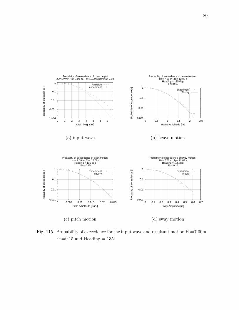
80
1e-04
0.001
0.01
0.1
1
0 1 2 3 4 5 6 7
prob
ablit
y of
exc
eede
nce
[-]
Crest height [m]
Probablity of exceedence of crest heightJONSWAP Hs= 7.00 m ,Tp= 12.09 s gamma= 2.00
Rayleighexperiment
(a) input wave
0.001
0.01
0.1
1
0 0.5 1 1.5 2 2.5
Pro
babl
ity o
f exc
eede
nce
[-]
Heave Amplitude [m]
Probablity of exceedence of heave motion Hs= 7.00 m ,Tp= 12.09 s
Heading = 135 deg Fn= 0.15
ExperimentTheory
(b) heave motion
0.001
0.01
0.1
1
0 0.005 0.01 0.015 0.02 0.025
Pro
babl
ity o
f exc
eede
nce
[-]
Pitch Amplitude [Rad.]
Probablity of exceedence of pitch motion Hs= 7.00 m ,Tp= 12.09 s
Heading = 135 deg Fn= 0.15
ExperimentTheory
(c) pitch motion
0.001
0.01
0.1
1
0 0.1 0.2 0.3 0.4 0.5 0.6 0.7
Pro
babl
ity o
f exc
eede
nce
[-]
Sway Amplitude [m]
Probablity of exceedence of sway motion Hs= 7.00 m ,Tp= 12.09 s
Heading = 135 deg Fn= 0.15
ExperimentTheory
(d) sway motion
Fig. 115. Probability of exceedence for the input wave and resultant motion Hs=7.00m,
Fn=0.15 and Heading = 135o
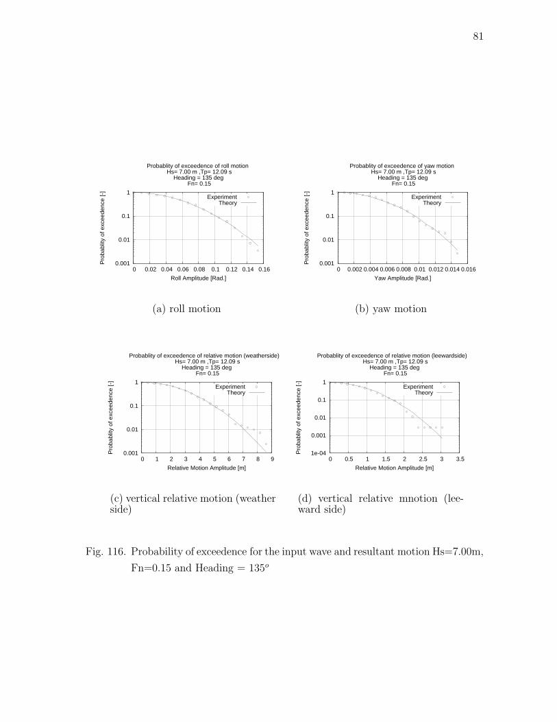
81
0.001
0.01
0.1
1
0 0.02 0.04 0.06 0.08 0.1 0.12 0.14 0.16
Pro
babl
ity o
f exc
eede
nce
[-]
Roll Amplitude [Rad.]
Probablity of exceedence of roll motion Hs= 7.00 m ,Tp= 12.09 s
Heading = 135 deg Fn= 0.15
ExperimentTheory
(a) roll motion
0.001
0.01
0.1
1
0 0.002 0.004 0.006 0.008 0.01 0.012 0.014 0.016
Pro
babl
ity o
f exc
eede
nce
[-]
Yaw Amplitude [Rad.]
Probablity of exceedence of yaw motion Hs= 7.00 m ,Tp= 12.09 s
Heading = 135 deg Fn= 0.15
ExperimentTheory
(b) yaw motion
0.001
0.01
0.1
1
0 1 2 3 4 5 6 7 8 9
Pro
babl
ity o
f exc
eede
nce
[-]
Relative Motion Amplitude [m]
Probablity of exceedence of relative motion (weatherside) Hs= 7.00 m ,Tp= 12.09 s
Heading = 135 deg Fn= 0.15
ExperimentTheory
(c) vertical relative motion (weatherside)
1e-04
0.001
0.01
0.1
1
0 0.5 1 1.5 2 2.5 3 3.5
Pro
babl
ity o
f exc
eede
nce
[-]
Relative Motion Amplitude [m]
Probablity of exceedence of relative motion (leewardside) Hs= 7.00 m ,Tp= 12.09 s
Heading = 135 deg Fn= 0.15
ExperimentTheory
(d) vertical relative mnotion (lee-ward side)
Fig. 116. Probability of exceedence for the input wave and resultant motion Hs=7.00m,
Fn=0.15 and Heading = 135o
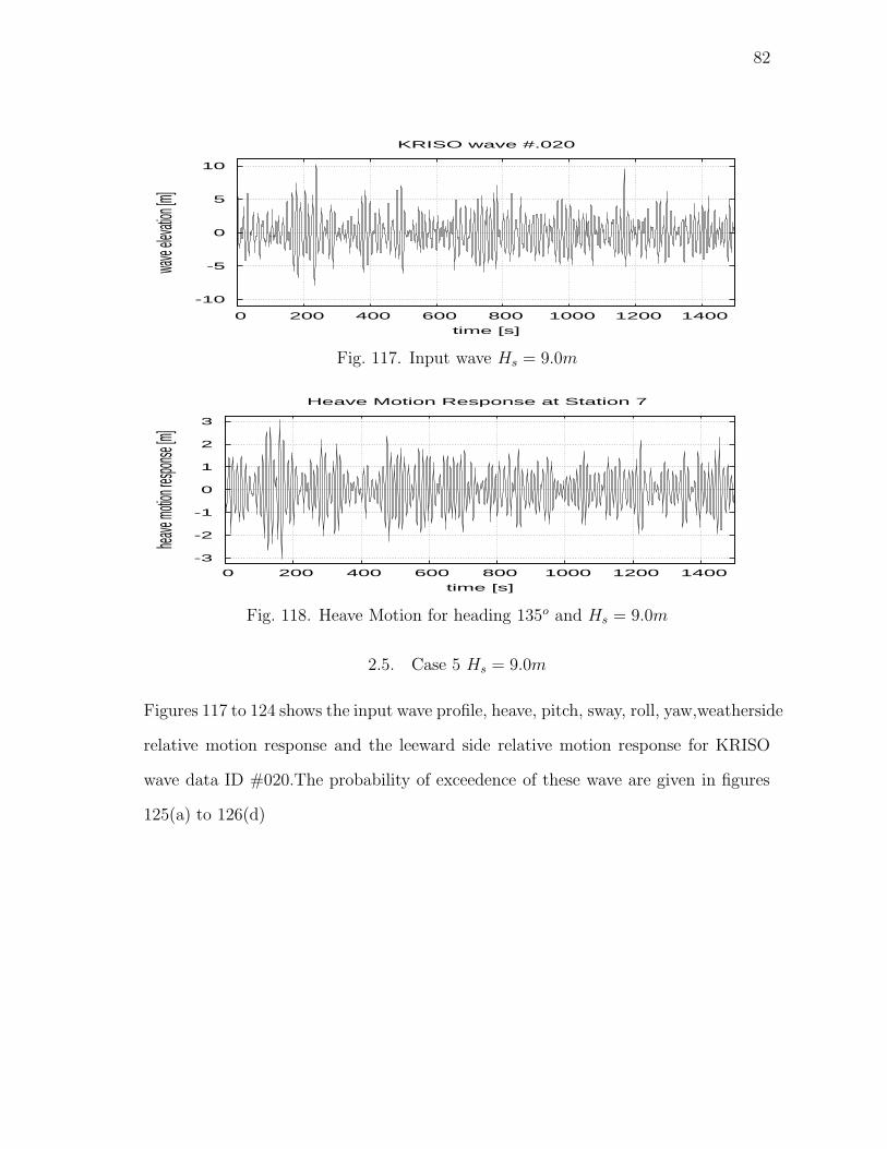
82
-10
-5
0
5
10
0 200 400 600 800 1000 1200 1400
wave
elevat
ion [m
]
time [s]
KRISO wave #.020
Fig. 117. Input wave Hs = 9.0m
-3
-2
-1
0
1
2
3
0 200 400 600 800 1000 1200 1400
heave
motion
respon
se [m]
time [s]
Heave Motion Response at Station 7
Fig. 118. Heave Motion for heading 135o and Hs = 9.0m
2.5. Case 5 Hs = 9.0m
Figures 117 to 124 shows the input wave profile, heave, pitch, sway, roll, yaw,weatherside
relative motion response and the leeward side relative motion response for KRISO
wave data ID #020.The probability of exceedence of these wave are given in figures
125(a) to 126(d)
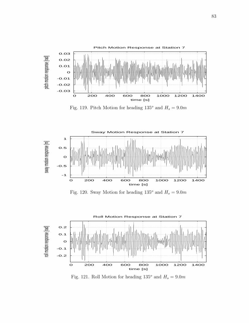
83
-0.03
-0.02
-0.01
0
0.01
0.02
0.03
0 200 400 600 800 1000 1200 1400
pitch m
otion re
sponse
[rad]
time [s]
Pitch Motion Response at Station 7
Fig. 119. Pitch Motion for heading 135o and Hs = 9.0m
-1
-0.5
0
0.5
1
0 200 400 600 800 1000 1200 1400
sway m
otion re
sponse
[m]
time [s]
Sway Motion Response at Station 7
Fig. 120. Sway Motion for heading 135o and Hs = 9.0m
-0.2
-0.1
0
0.1
0.2
0 200 400 600 800 1000 1200 1400
roll mo
tion res
ponse
[rad]
time [s]
Roll Motion Response at Station 7
Fig. 121. Roll Motion for heading 135o and Hs = 9.0m
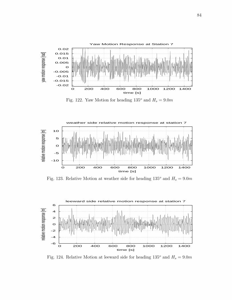
84
-0.02
-0.015
-0.01
-0.005
0
0.005
0.01
0.015
0.02
0 200 400 600 800 1000 1200 1400
yaw mo
tion res
ponse
[rad]
time [s]
Yaw Motion Response at Station 7
Fig. 122. Yaw Motion for heading 135o and Hs = 9.0m
-10
-5
0
5
10
0 200 400 600 800 1000 1200 1400
relative
motion
respon
se [m]
time [s]
weather side relative motion response at station 7
Fig. 123. Relative Motion at weather side for heading 135o and Hs = 9.0m
-6
-4
-2
0
2
4
6
0 200 400 600 800 1000 1200 1400
relative
motion
respon
se [m]
time [s]
leeward side relative motion response at station 7
Fig. 124. Relative Motion at leeward side for heading 135o and Hs = 9.0m
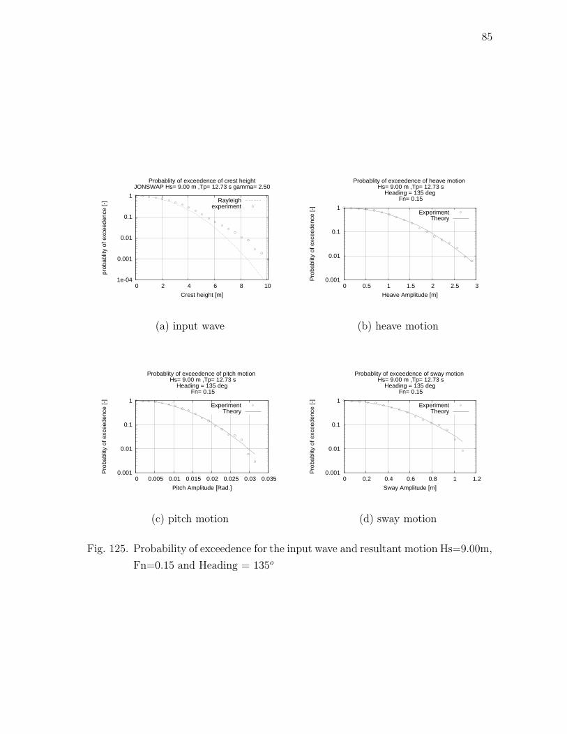
85
1e-04
0.001
0.01
0.1
1
0 2 4 6 8 10
prob
ablit
y of
exc
eede
nce
[-]
Crest height [m]
Probablity of exceedence of crest heightJONSWAP Hs= 9.00 m ,Tp= 12.73 s gamma= 2.50
Rayleighexperiment
(a) input wave
0.001
0.01
0.1
1
0 0.5 1 1.5 2 2.5 3
Pro
babl
ity o
f exc
eede
nce
[-]
Heave Amplitude [m]
Probablity of exceedence of heave motion Hs= 9.00 m ,Tp= 12.73 s
Heading = 135 deg Fn= 0.15
ExperimentTheory
(b) heave motion
0.001
0.01
0.1
1
0 0.005 0.01 0.015 0.02 0.025 0.03 0.035
Pro
babl
ity o
f exc
eede
nce
[-]
Pitch Amplitude [Rad.]
Probablity of exceedence of pitch motion Hs= 9.00 m ,Tp= 12.73 s
Heading = 135 deg Fn= 0.15
ExperimentTheory
(c) pitch motion
0.001
0.01
0.1
1
0 0.2 0.4 0.6 0.8 1 1.2
Pro
babl
ity o
f exc
eede
nce
[-]
Sway Amplitude [m]
Probablity of exceedence of sway motion Hs= 9.00 m ,Tp= 12.73 s
Heading = 135 deg Fn= 0.15
ExperimentTheory
(d) sway motion
Fig. 125. Probability of exceedence for the input wave and resultant motion Hs=9.00m,
Fn=0.15 and Heading = 135o
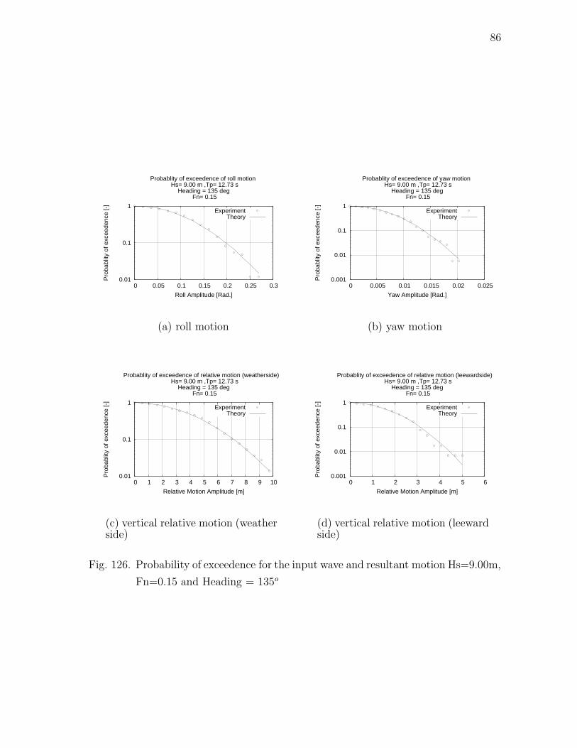
86
0.01
0.1
1
0 0.05 0.1 0.15 0.2 0.25 0.3
Pro
babl
ity o
f exc
eede
nce
[-]
Roll Amplitude [Rad.]
Probablity of exceedence of roll motion Hs= 9.00 m ,Tp= 12.73 s
Heading = 135 deg Fn= 0.15
ExperimentTheory
(a) roll motion
0.001
0.01
0.1
1
0 0.005 0.01 0.015 0.02 0.025
Pro
babl
ity o
f exc
eede
nce
[-]
Yaw Amplitude [Rad.]
Probablity of exceedence of yaw motion Hs= 9.00 m ,Tp= 12.73 s
Heading = 135 deg Fn= 0.15
ExperimentTheory
(b) yaw motion
0.01
0.1
1
0 1 2 3 4 5 6 7 8 9 10
Pro
babl
ity o
f exc
eede
nce
[-]
Relative Motion Amplitude [m]
Probablity of exceedence of relative motion (weatherside) Hs= 9.00 m ,Tp= 12.73 s
Heading = 135 deg Fn= 0.15
ExperimentTheory
(c) vertical relative motion (weatherside)
0.001
0.01
0.1
1
0 1 2 3 4 5 6
Pro
babl
ity o
f exc
eede
nce
[-]
Relative Motion Amplitude [m]
Probablity of exceedence of relative motion (leewardside) Hs= 9.00 m ,Tp= 12.73 s
Heading = 135 deg Fn= 0.15
ExperimentTheory
(d) vertical relative motion (leewardside)
Fig. 126. Probability of exceedence for the input wave and resultant motion Hs=9.00m,
Fn=0.15 and Heading = 135o
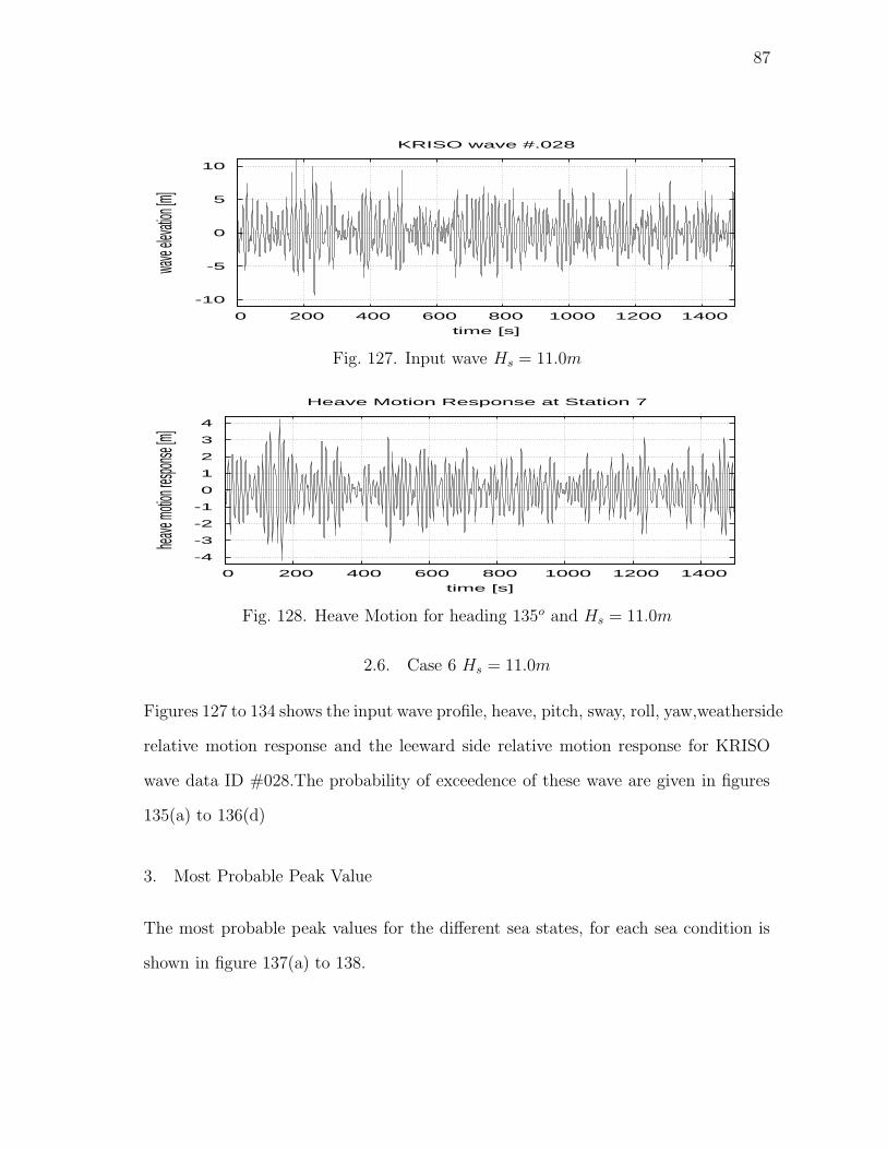
87
-10
-5
0
5
10
0 200 400 600 800 1000 1200 1400
wave
elevat
ion [m
]
time [s]
KRISO wave #.028
Fig. 127. Input wave Hs = 11.0m
-4
-3
-2
-1
0
1
2
3
4
0 200 400 600 800 1000 1200 1400
heave
motion
respon
se [m]
time [s]
Heave Motion Response at Station 7
Fig. 128. Heave Motion for heading 135o and Hs = 11.0m
2.6. Case 6 Hs = 11.0m
Figures 127 to 134 shows the input wave profile, heave, pitch, sway, roll, yaw,weatherside
relative motion response and the leeward side relative motion response for KRISO
wave data ID #028.The probability of exceedence of these wave are given in figures
135(a) to 136(d)
3. Most Probable Peak Value
The most probable peak values for the different sea states, for each sea condition is
shown in figure 137(a) to 138.
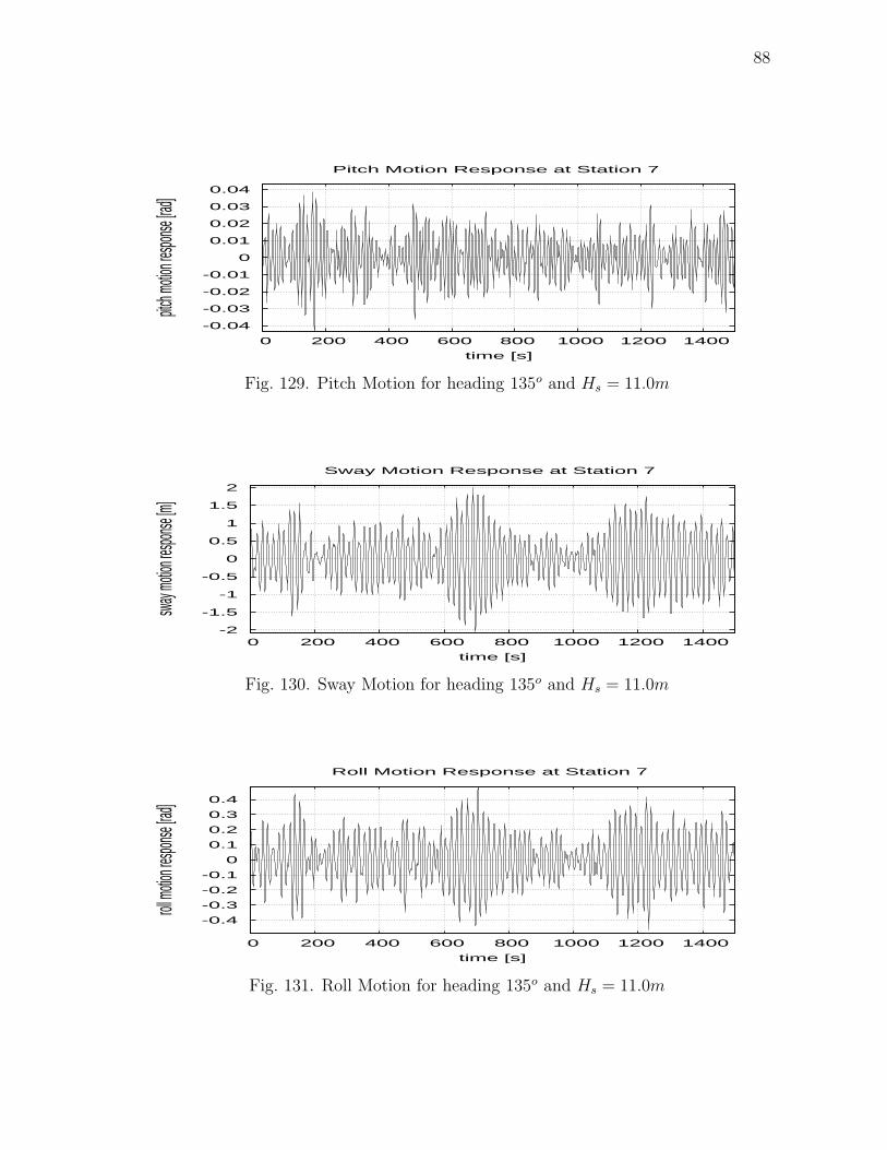
88
-0.04
-0.03
-0.02
-0.01
0
0.01
0.02
0.03
0.04
0 200 400 600 800 1000 1200 1400
pitch m
otion re
sponse
[rad]
time [s]
Pitch Motion Response at Station 7
Fig. 129. Pitch Motion for heading 135o and Hs = 11.0m
-2
-1.5
-1
-0.5
0
0.5
1
1.5
2
0 200 400 600 800 1000 1200 1400
sway m
otion re
sponse
[m]
time [s]
Sway Motion Response at Station 7
Fig. 130. Sway Motion for heading 135o and Hs = 11.0m
-0.4
-0.3
-0.2
-0.1
0
0.1
0.2
0.3
0.4
0 200 400 600 800 1000 1200 1400
roll mo
tion res
ponse
[rad]
time [s]
Roll Motion Response at Station 7
Fig. 131. Roll Motion for heading 135o and Hs = 11.0m
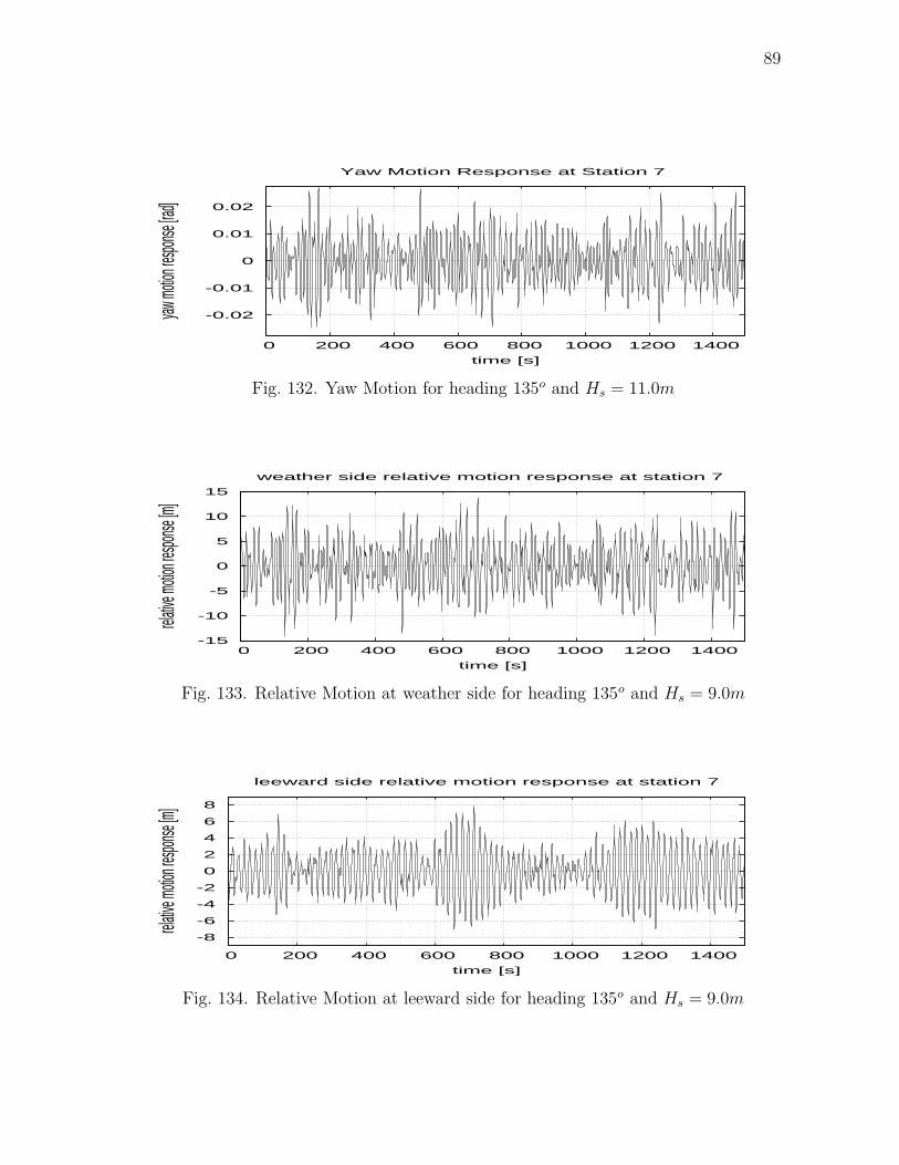
89
-0.02
-0.01
0
0.01
0.02
0 200 400 600 800 1000 1200 1400
yaw mo
tion res
ponse
[rad]
time [s]
Yaw Motion Response at Station 7
Fig. 132. Yaw Motion for heading 135o and Hs = 11.0m
-15
-10
-5
0
5
10
15
0 200 400 600 800 1000 1200 1400
relative
motion
respon
se [m]
time [s]
weather side relative motion response at station 7
Fig. 133. Relative Motion at weather side for heading 135o and Hs = 9.0m
-8
-6
-4
-2
0
2
4
6
8
0 200 400 600 800 1000 1200 1400
relative
motion
respon
se [m]
time [s]
leeward side relative motion response at station 7
Fig. 134. Relative Motion at leeward side for heading 135o and Hs = 9.0m
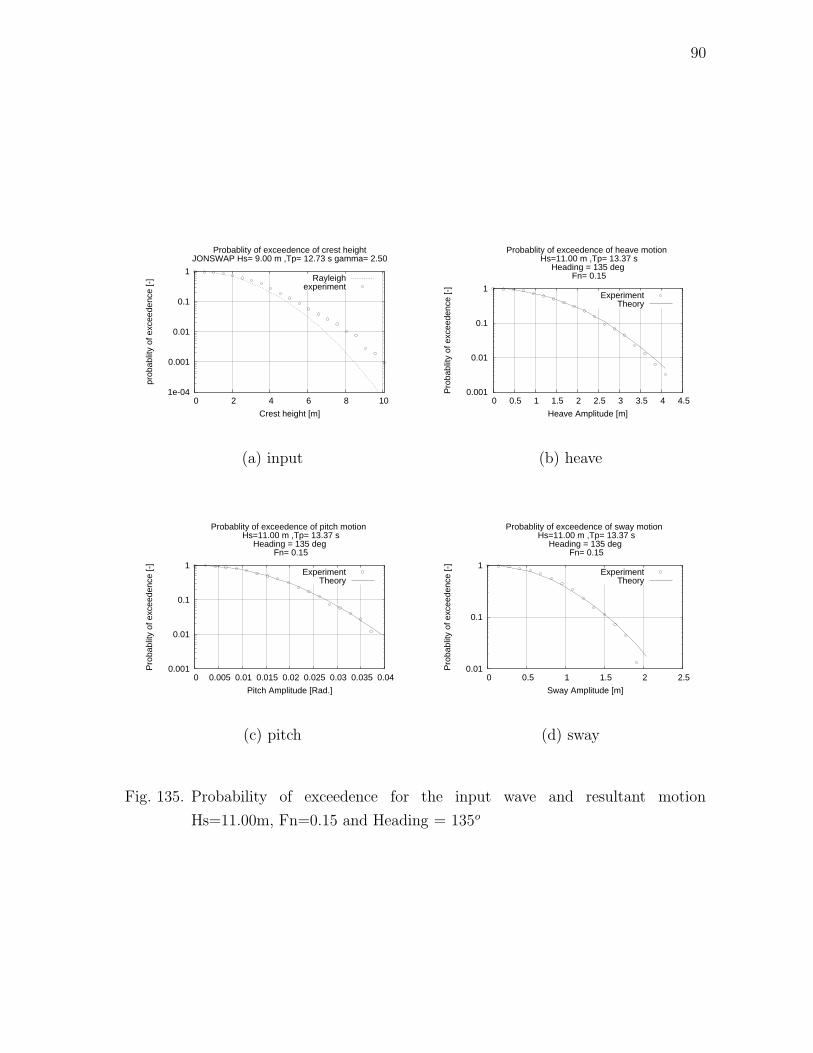
90
1e-04
0.001
0.01
0.1
1
0 2 4 6 8 10
prob
ablit
y of
exc
eede
nce
[-]
Crest height [m]
Probablity of exceedence of crest heightJONSWAP Hs= 9.00 m ,Tp= 12.73 s gamma= 2.50
Rayleighexperiment
(a) input
0.001
0.01
0.1
1
0 0.5 1 1.5 2 2.5 3 3.5 4 4.5
Pro
babl
ity o
f exc
eede
nce
[-]
Heave Amplitude [m]
Probablity of exceedence of heave motion Hs=11.00 m ,Tp= 13.37 s
Heading = 135 deg Fn= 0.15
ExperimentTheory
(b) heave
0.001
0.01
0.1
1
0 0.005 0.01 0.015 0.02 0.025 0.03 0.035 0.04
Pro
babl
ity o
f exc
eede
nce
[-]
Pitch Amplitude [Rad.]
Probablity of exceedence of pitch motion Hs=11.00 m ,Tp= 13.37 s
Heading = 135 deg Fn= 0.15
ExperimentTheory
(c) pitch
0.01
0.1
1
0 0.5 1 1.5 2 2.5
Pro
babl
ity o
f exc
eede
nce
[-]
Sway Amplitude [m]
Probablity of exceedence of sway motion Hs=11.00 m ,Tp= 13.37 s
Heading = 135 deg Fn= 0.15
ExperimentTheory
(d) sway
Fig. 135. Probability of exceedence for the input wave and resultant motion
Hs=11.00m, Fn=0.15 and Heading = 135o
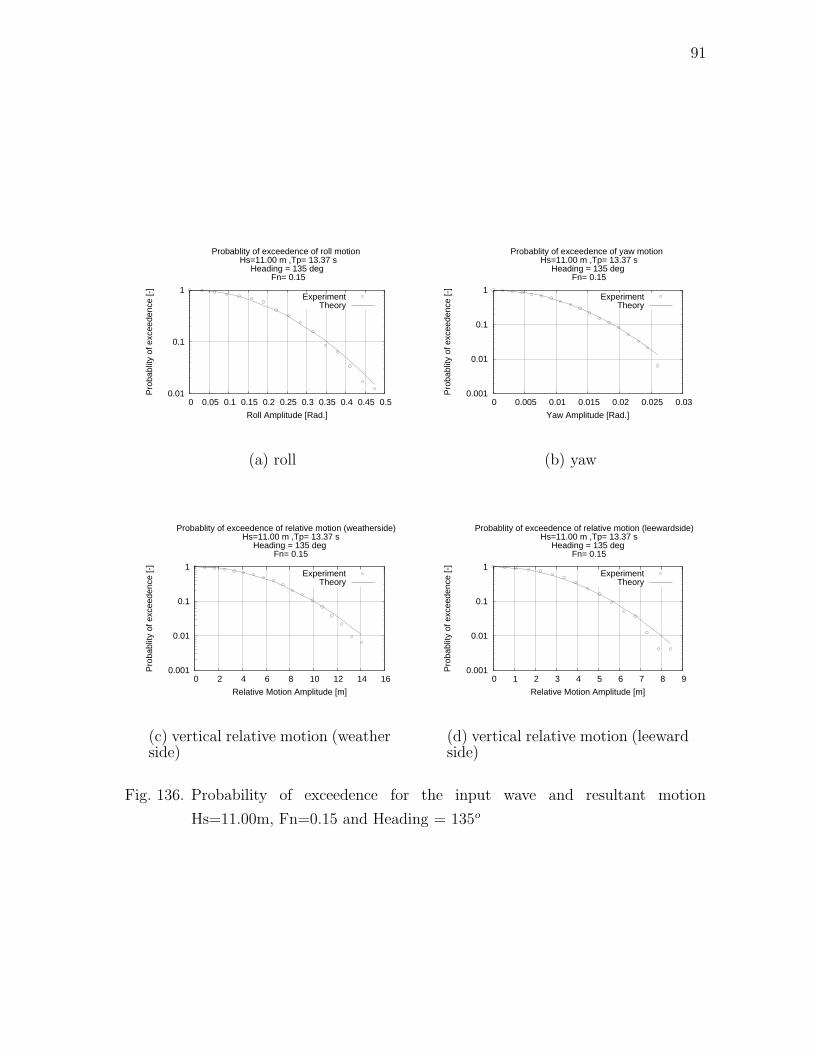
91
0.01
0.1
1
0 0.05 0.1 0.15 0.2 0.25 0.3 0.35 0.4 0.45 0.5
Pro
babl
ity o
f exc
eede
nce
[-]
Roll Amplitude [Rad.]
Probablity of exceedence of roll motion Hs=11.00 m ,Tp= 13.37 s
Heading = 135 deg Fn= 0.15
ExperimentTheory
(a) roll
0.001
0.01
0.1
1
0 0.005 0.01 0.015 0.02 0.025 0.03
Pro
babl
ity o
f exc
eede
nce
[-]
Yaw Amplitude [Rad.]
Probablity of exceedence of yaw motion Hs=11.00 m ,Tp= 13.37 s
Heading = 135 deg Fn= 0.15
ExperimentTheory
(b) yaw
0.001
0.01
0.1
1
0 2 4 6 8 10 12 14 16
Pro
babl
ity o
f exc
eede
nce
[-]
Relative Motion Amplitude [m]
Probablity of exceedence of relative motion (weatherside) Hs=11.00 m ,Tp= 13.37 s
Heading = 135 deg Fn= 0.15
ExperimentTheory
(c) vertical relative motion (weatherside)
0.001
0.01
0.1
1
0 1 2 3 4 5 6 7 8 9
Pro
babl
ity o
f exc
eede
nce
[-]
Relative Motion Amplitude [m]
Probablity of exceedence of relative motion (leewardside) Hs=11.00 m ,Tp= 13.37 s
Heading = 135 deg Fn= 0.15
ExperimentTheory
(d) vertical relative motion (leewardside)
Fig. 136. Probability of exceedence for the input wave and resultant motion
Hs=11.00m, Fn=0.15 and Heading = 135o
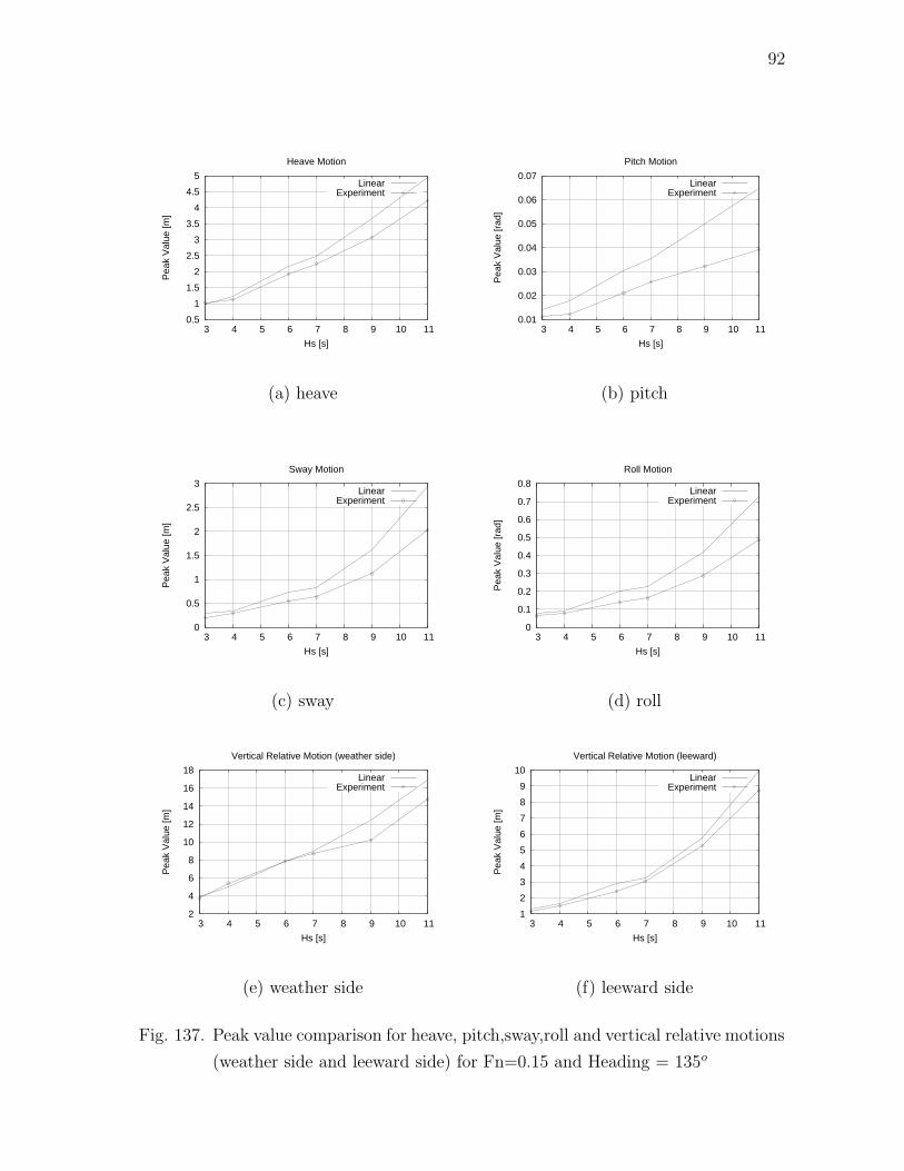
92
0.5
1
1.5
2
2.5
3
3.5
4
4.5
5
3 4 5 6 7 8 9 10 11
Pea
k V
alue
[m]
Hs [s]
Heave Motion
LinearExperiment
(a) heave
0.01
0.02
0.03
0.04
0.05
0.06
0.07
3 4 5 6 7 8 9 10 11
Pea
k V
alue
[rad
]
Hs [s]
Pitch Motion
LinearExperiment
(b) pitch
0
0.5
1
1.5
2
2.5
3
3 4 5 6 7 8 9 10 11
Pea
k V
alue
[m]
Hs [s]
Sway Motion
LinearExperiment
(c) sway
0
0.1
0.2
0.3
0.4
0.5
0.6
0.7
0.8
3 4 5 6 7 8 9 10 11
Pea
k V
alue
[rad
]
Hs [s]
Roll Motion
LinearExperiment
(d) roll
2
4
6
8
10
12
14
16
18
3 4 5 6 7 8 9 10 11
Pea
k V
alue
[m]
Hs [s]
Vertical Relative Motion (weather side)
LinearExperiment
(e) weather side
1
2
3
4
5
6
7
8
9
10
3 4 5 6 7 8 9 10 11
Pea
k V
alue
[m]
Hs [s]
Vertical Relative Motion (leeward)
LinearExperiment
(f) leeward side
Fig. 137. Peak value comparison for heave, pitch,sway,roll and vertical relative motions
(weather side and leeward side) for Fn=0.15 and Heading = 135o
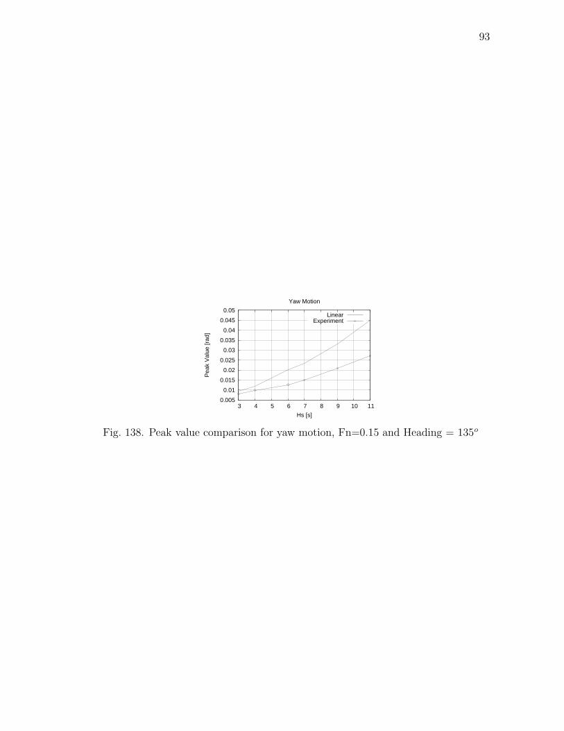
93
0.005
0.01
0.015
0.02
0.025
0.03
0.035
0.04
0.045
0.05
3 4 5 6 7 8 9 10 11
Pea
k V
alue
[rad
]
Hs [s]
Yaw Motion
LinearExperiment
Fig. 138. Peak value comparison for yaw motion, Fn=0.15 and Heading = 135o
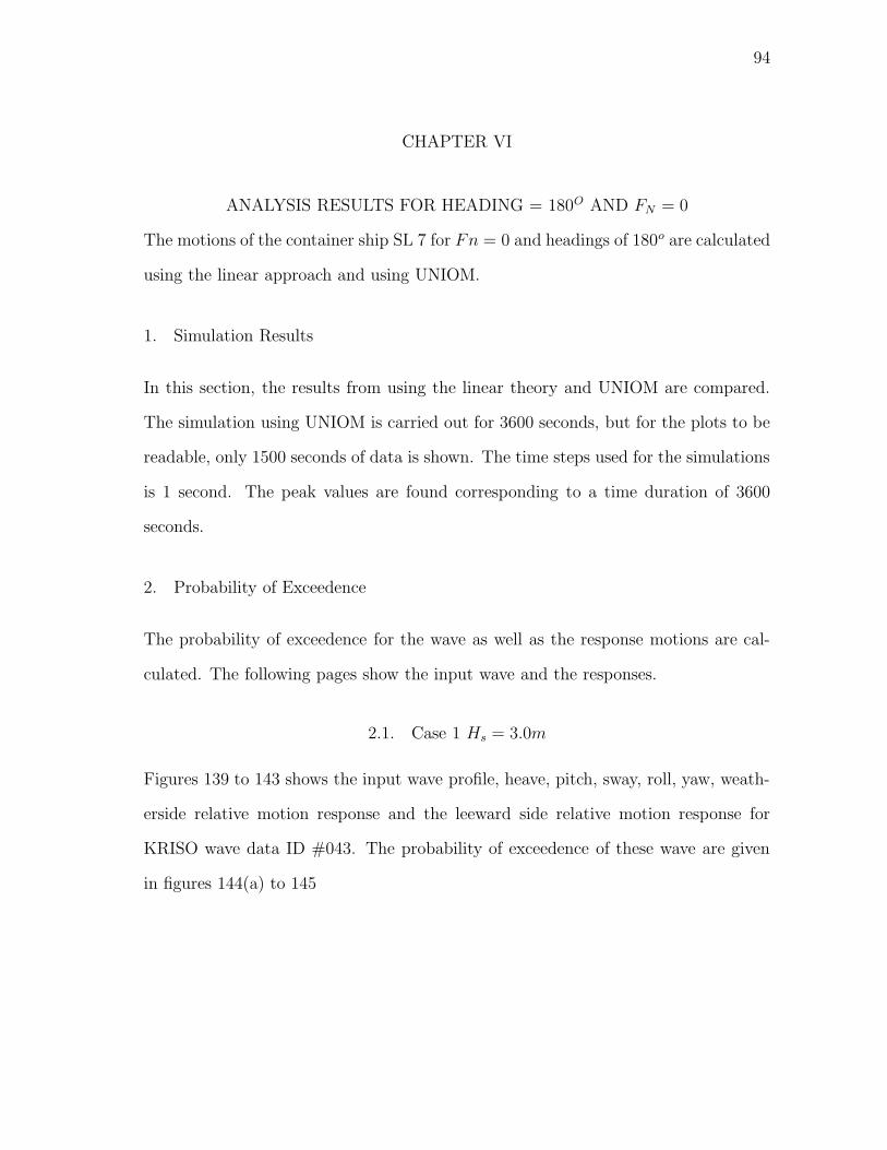
94
CHAPTER VI
ANALYSIS RESULTS FOR HEADING = 180O AND FN = 0
The motions of the container ship SL 7 for Fn = 0 and headings of 180o are calculated
using the linear approach and using UNIOM.
1. Simulation Results
In this section, the results from using the linear theory and UNIOM are compared.
The simulation using UNIOM is carried out for 3600 seconds, but for the plots to be
readable, only 1500 seconds of data is shown. The time steps used for the simulations
is 1 second. The peak values are found corresponding to a time duration of 3600
seconds.
2. Probability of Exceedence
The probability of exceedence for the wave as well as the response motions are cal-
culated. The following pages show the input wave and the responses.
2.1. Case 1 Hs = 3.0m
Figures 139 to 143 shows the input wave profile, heave, pitch, sway, roll, yaw, weath-
erside relative motion response and the leeward side relative motion response for
KRISO wave data ID #043. The probability of exceedence of these wave are given
in figures 144(a) to 145
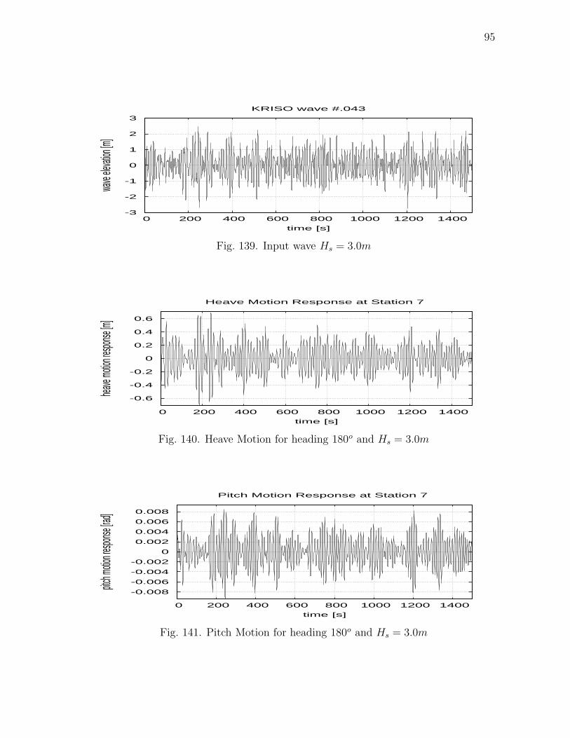
95
-3
-2
-1
0
1
2
3
0 200 400 600 800 1000 1200 1400
wave
elevat
ion [m
]
time [s]
KRISO wave #.043
Fig. 139. Input wave Hs = 3.0m
-0.6
-0.4
-0.2
0
0.2
0.4
0.6
0 200 400 600 800 1000 1200 1400
heave
motion
respon
se [m]
time [s]
Heave Motion Response at Station 7
Fig. 140. Heave Motion for heading 180o and Hs = 3.0m
-0.008
-0.006
-0.004
-0.002
0
0.002
0.004
0.006
0.008
0 200 400 600 800 1000 1200 1400
pitch m
otion re
sponse
[rad]
time [s]
Pitch Motion Response at Station 7
Fig. 141. Pitch Motion for heading 180o and Hs = 3.0m
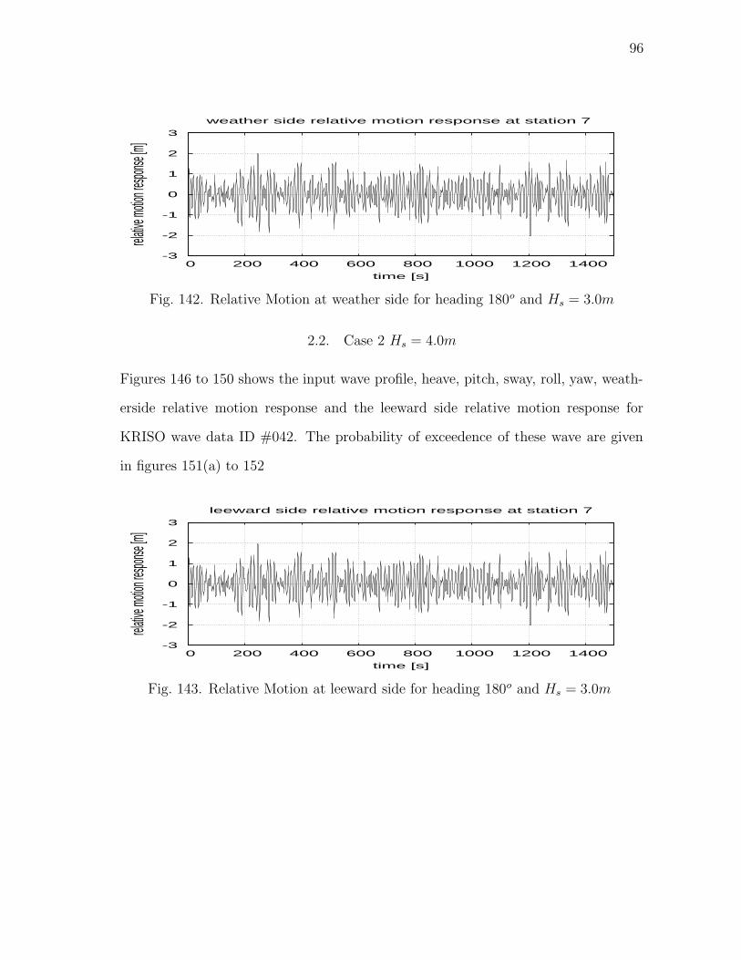
96
-3
-2
-1
0
1
2
3
0 200 400 600 800 1000 1200 1400
relative
motion
respon
se [m]
time [s]
weather side relative motion response at station 7
Fig. 142. Relative Motion at weather side for heading 180o and Hs = 3.0m
2.2. Case 2 Hs = 4.0m
Figures 146 to 150 shows the input wave profile, heave, pitch, sway, roll, yaw, weath-
erside relative motion response and the leeward side relative motion response for
KRISO wave data ID #042. The probability of exceedence of these wave are given
in figures 151(a) to 152
-3
-2
-1
0
1
2
3
0 200 400 600 800 1000 1200 1400
relative
motion
respon
se [m]
time [s]
leeward side relative motion response at station 7
Fig. 143. Relative Motion at leeward side for heading 180o and Hs = 3.0m
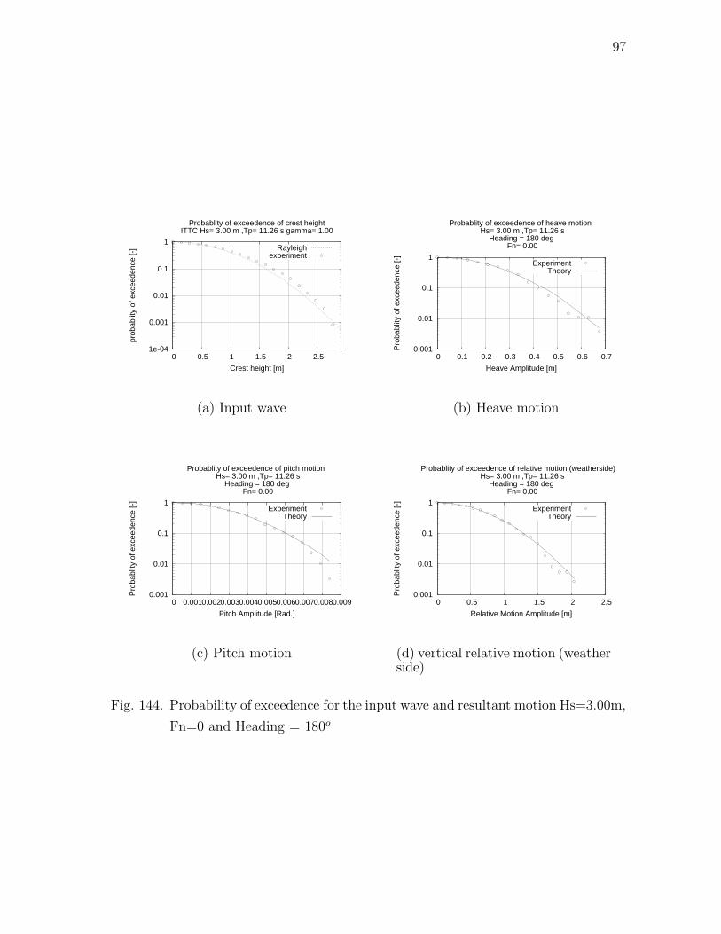
97
1e-04
0.001
0.01
0.1
1
0 0.5 1 1.5 2 2.5
prob
ablit
y of
exc
eede
nce
[-]
Crest height [m]
Probablity of exceedence of crest heightITTC Hs= 3.00 m ,Tp= 11.26 s gamma= 1.00
Rayleighexperiment
(a) Input wave
0.001
0.01
0.1
1
0 0.1 0.2 0.3 0.4 0.5 0.6 0.7
Pro
babl
ity o
f exc
eede
nce
[-]
Heave Amplitude [m]
Probablity of exceedence of heave motion Hs= 3.00 m ,Tp= 11.26 s
Heading = 180 deg Fn= 0.00
ExperimentTheory
(b) Heave motion
0.001
0.01
0.1
1
0 0.001 0.002 0.003 0.004 0.005 0.006 0.007 0.008 0.009
Pro
babl
ity o
f exc
eede
nce
[-]
Pitch Amplitude [Rad.]
Probablity of exceedence of pitch motion Hs= 3.00 m ,Tp= 11.26 s
Heading = 180 deg Fn= 0.00
ExperimentTheory
(c) Pitch motion
0.001
0.01
0.1
1
0 0.5 1 1.5 2 2.5
Pro
babl
ity o
f exc
eede
nce
[-]
Relative Motion Amplitude [m]
Probablity of exceedence of relative motion (weatherside) Hs= 3.00 m ,Tp= 11.26 s
Heading = 180 deg Fn= 0.00
ExperimentTheory
(d) vertical relative motion (weatherside)
Fig. 144. Probability of exceedence for the input wave and resultant motion Hs=3.00m,
Fn=0 and Heading = 180o
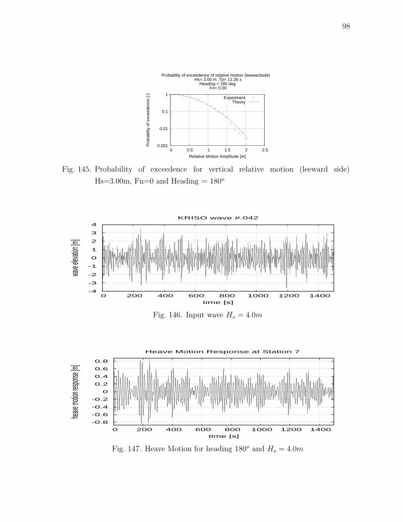
98
0.001
0.01
0.1
1
0 0.5 1 1.5 2 2.5P
roba
blity
of e
xcee
denc
e [-
]
Relative Motion Amplitude [m]
Probablity of exceedence of relative motion (leewardside) Hs= 3.00 m ,Tp= 11.26 s
Heading = 180 deg Fn= 0.00
ExperimentTheory
Fig. 145. Probability of exceedence for vertical relative motion (leeward side)
Hs=3.00m, Fn=0 and Heading = 180o
-4
-3
-2
-1
0
1
2
3
4
0 200 400 600 800 1000 1200 1400
wave
elevat
ion [m
]
time [s]
KRISO wave #.042
Fig. 146. Input wave Hs = 4.0m
-0.8
-0.6
-0.4
-0.2
0
0.2
0.4
0.6
0.8
0 200 400 600 800 1000 1200 1400
heave
motion
respon
se [m]
time [s]
Heave Motion Response at Station 7
Fig. 147. Heave Motion for heading 180o and Hs = 4.0m
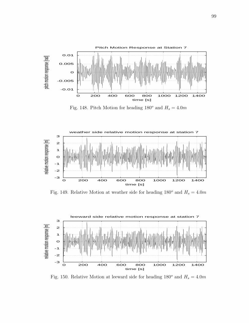
99
-0.01
-0.005
0
0.005
0.01
0 200 400 600 800 1000 1200 1400
pitch m
otion re
sponse
[rad]
time [s]
Pitch Motion Response at Station 7
Fig. 148. Pitch Motion for heading 180o and Hs = 4.0m
-3
-2
-1
0
1
2
3
0 200 400 600 800 1000 1200 1400
relative
motion
respon
se [m]
time [s]
weather side relative motion response at station 7
Fig. 149. Relative Motion at weather side for heading 180o and Hs = 4.0m
-3
-2
-1
0
1
2
3
0 200 400 600 800 1000 1200 1400
relative
motion
respon
se [m]
time [s]
leeward side relative motion response at station 7
Fig. 150. Relative Motion at leeward side for heading 180o and Hs = 4.0m
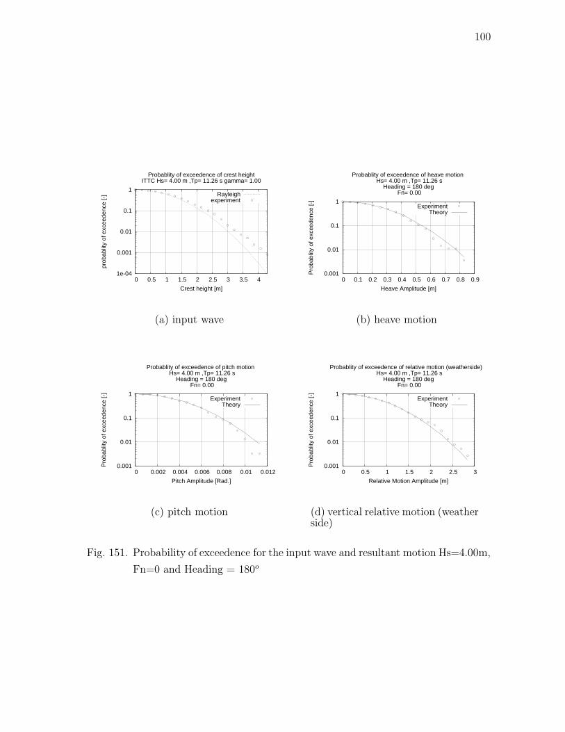
100
1e-04
0.001
0.01
0.1
1
0 0.5 1 1.5 2 2.5 3 3.5 4
prob
ablit
y of
exc
eede
nce
[-]
Crest height [m]
Probablity of exceedence of crest heightITTC Hs= 4.00 m ,Tp= 11.26 s gamma= 1.00
Rayleighexperiment
(a) input wave
0.001
0.01
0.1
1
0 0.1 0.2 0.3 0.4 0.5 0.6 0.7 0.8 0.9
Pro
babl
ity o
f exc
eede
nce
[-]
Heave Amplitude [m]
Probablity of exceedence of heave motion Hs= 4.00 m ,Tp= 11.26 s
Heading = 180 deg Fn= 0.00
ExperimentTheory
(b) heave motion
0.001
0.01
0.1
1
0 0.002 0.004 0.006 0.008 0.01 0.012
Pro
babl
ity o
f exc
eede
nce
[-]
Pitch Amplitude [Rad.]
Probablity of exceedence of pitch motion Hs= 4.00 m ,Tp= 11.26 s
Heading = 180 deg Fn= 0.00
ExperimentTheory
(c) pitch motion
0.001
0.01
0.1
1
0 0.5 1 1.5 2 2.5 3
Pro
babl
ity o
f exc
eede
nce
[-]
Relative Motion Amplitude [m]
Probablity of exceedence of relative motion (weatherside) Hs= 4.00 m ,Tp= 11.26 s
Heading = 180 deg Fn= 0.00
ExperimentTheory
(d) vertical relative motion (weatherside)
Fig. 151. Probability of exceedence for the input wave and resultant motion Hs=4.00m,
Fn=0 and Heading = 180o
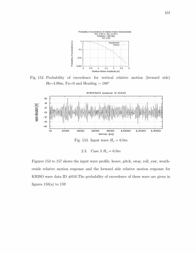
101
0.001
0.01
0.1
1
0 0.5 1 1.5 2 2.5 3
Pro
babl
ity o
f exc
eede
nce
[-]
Relative Motion Amplitude [m]
Probablity of exceedence of relative motion (leewardside) Hs= 4.00 m ,Tp= 11.26 s
Heading = 180 deg Fn= 0.00
ExperimentTheory
Fig. 152. Probability of exceedence for vertical relative motion (leeward side)
Hs=4.00m, Fn=0 and Heading = 180o
-6
-4
-2
0
2
4
6
0 200 400 600 800 1000 1200 1400
wave
elevat
ion [m
]
time [s]
KRISO wave #.010
Fig. 153. Input wave Hs = 6.0m
2.3. Case 3 Hs = 6.0m
Figures 153 to 157 shows the input wave profile, heave, pitch, sway, roll, yaw, weath-
erside relative motion response and the leeward side relative motion response for
KRISO wave data ID #010.The probability of exceedence of these wave are given in
figures 158(a) to 159
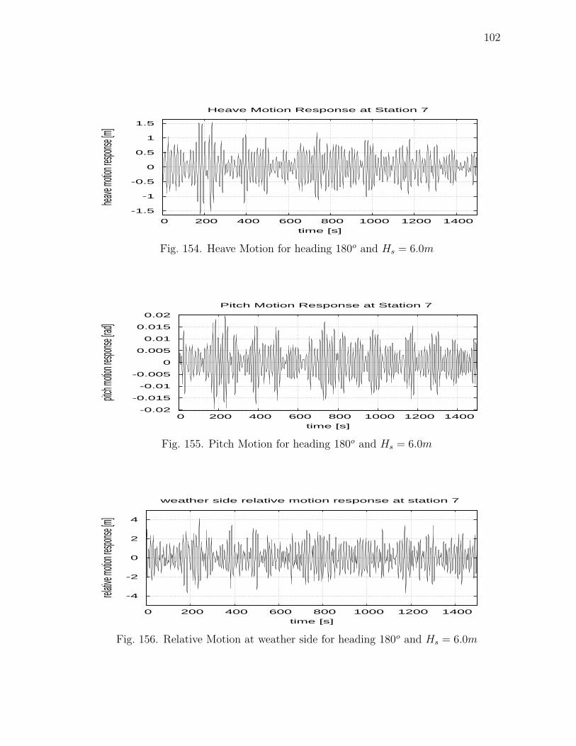
102
-1.5
-1
-0.5
0
0.5
1
1.5
0 200 400 600 800 1000 1200 1400
heave
motion
respon
se [m]
time [s]
Heave Motion Response at Station 7
Fig. 154. Heave Motion for heading 180o and Hs = 6.0m
-0.02
-0.015
-0.01
-0.005
0
0.005
0.01
0.015
0.02
0 200 400 600 800 1000 1200 1400
pitch m
otion re
sponse
[rad]
time [s]
Pitch Motion Response at Station 7
Fig. 155. Pitch Motion for heading 180o and Hs = 6.0m
-4
-2
0
2
4
0 200 400 600 800 1000 1200 1400
relative
motion
respon
se [m]
time [s]
weather side relative motion response at station 7
Fig. 156. Relative Motion at weather side for heading 180o and Hs = 6.0m
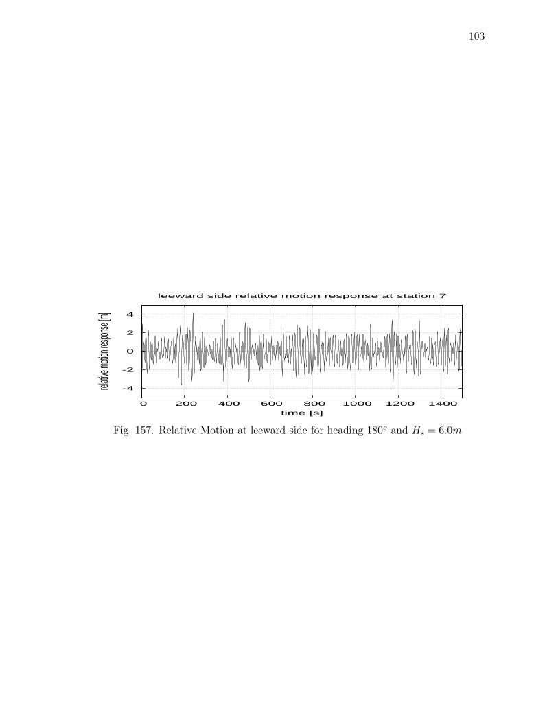
103
-4
-2
0
2
4
0 200 400 600 800 1000 1200 1400
relative
motion
respon
se [m]
time [s]
leeward side relative motion response at station 7
Fig. 157. Relative Motion at leeward side for heading 180o and Hs = 6.0m
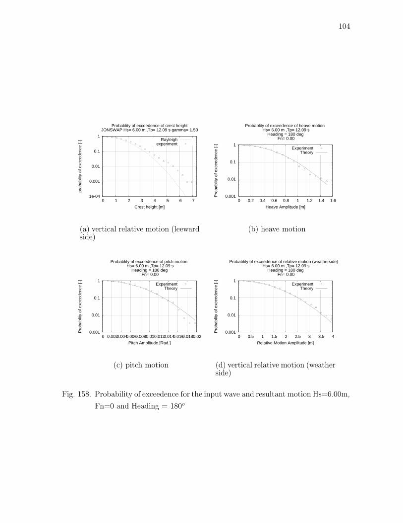
104
1e-04
0.001
0.01
0.1
1
0 1 2 3 4 5 6 7
prob
ablit
y of
exc
eede
nce
[-]
Crest height [m]
Probablity of exceedence of crest heightJONSWAP Hs= 6.00 m ,Tp= 12.09 s gamma= 1.50
Rayleighexperiment
(a) vertical relative motion (leewardside)
0.001
0.01
0.1
1
0 0.2 0.4 0.6 0.8 1 1.2 1.4 1.6
Pro
babl
ity o
f exc
eede
nce
[-]
Heave Amplitude [m]
Probablity of exceedence of heave motion Hs= 6.00 m ,Tp= 12.09 s
Heading = 180 deg Fn= 0.00
ExperimentTheory
(b) heave motion
0.001
0.01
0.1
1
0 0.002 0.004 0.006 0.008 0.01 0.012 0.014 0.016 0.018 0.02
Pro
babl
ity o
f exc
eede
nce
[-]
Pitch Amplitude [Rad.]
Probablity of exceedence of pitch motion Hs= 6.00 m ,Tp= 12.09 s
Heading = 180 deg Fn= 0.00
ExperimentTheory
(c) pitch motion
0.001
0.01
0.1
1
0 0.5 1 1.5 2 2.5 3 3.5 4
Pro
babl
ity o
f exc
eede
nce
[-]
Relative Motion Amplitude [m]
Probablity of exceedence of relative motion (weatherside) Hs= 6.00 m ,Tp= 12.09 s
Heading = 180 deg Fn= 0.00
ExperimentTheory
(d) vertical relative motion (weatherside)
Fig. 158. Probability of exceedence for the input wave and resultant motion Hs=6.00m,
Fn=0 and Heading = 180o
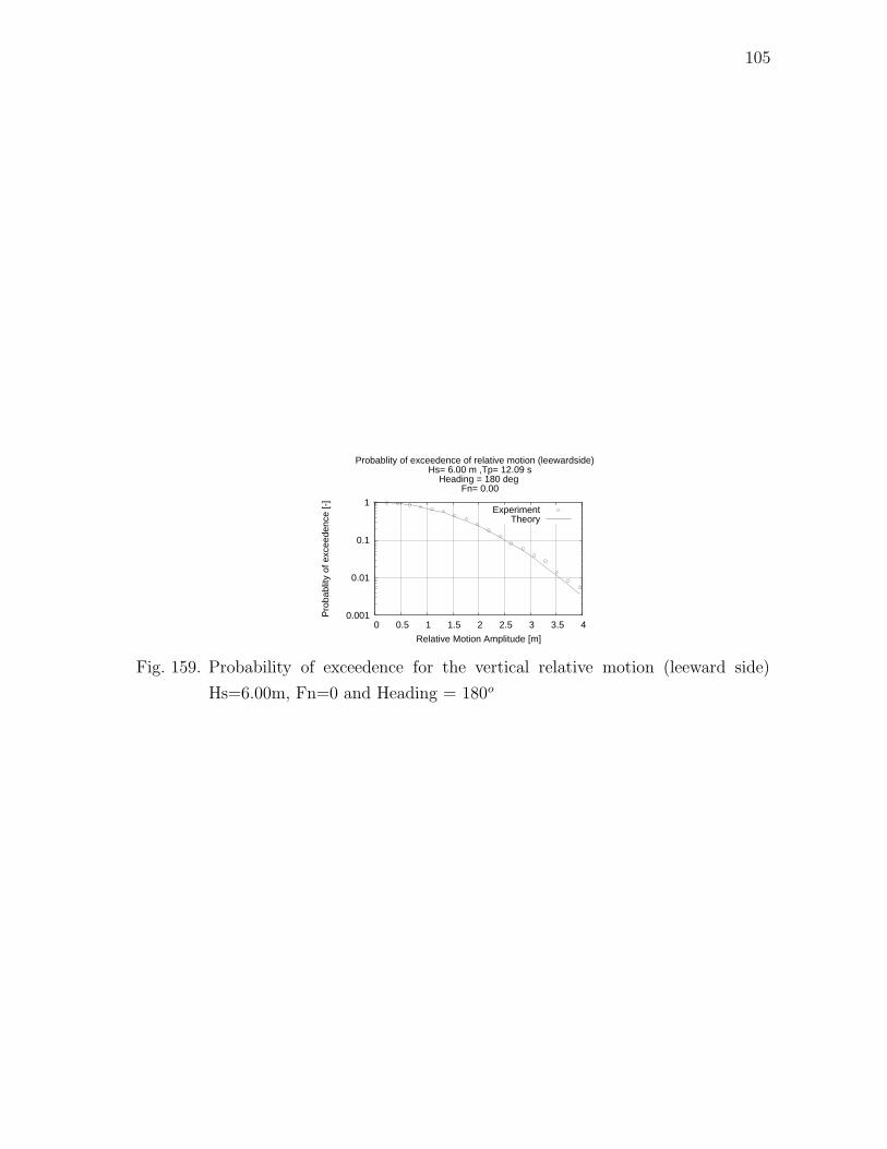
105
0.001
0.01
0.1
1
0 0.5 1 1.5 2 2.5 3 3.5 4
Pro
babl
ity o
f exc
eede
nce
[-]
Relative Motion Amplitude [m]
Probablity of exceedence of relative motion (leewardside) Hs= 6.00 m ,Tp= 12.09 s
Heading = 180 deg Fn= 0.00
ExperimentTheory
Fig. 159. Probability of exceedence for the vertical relative motion (leeward side)
Hs=6.00m, Fn=0 and Heading = 180o
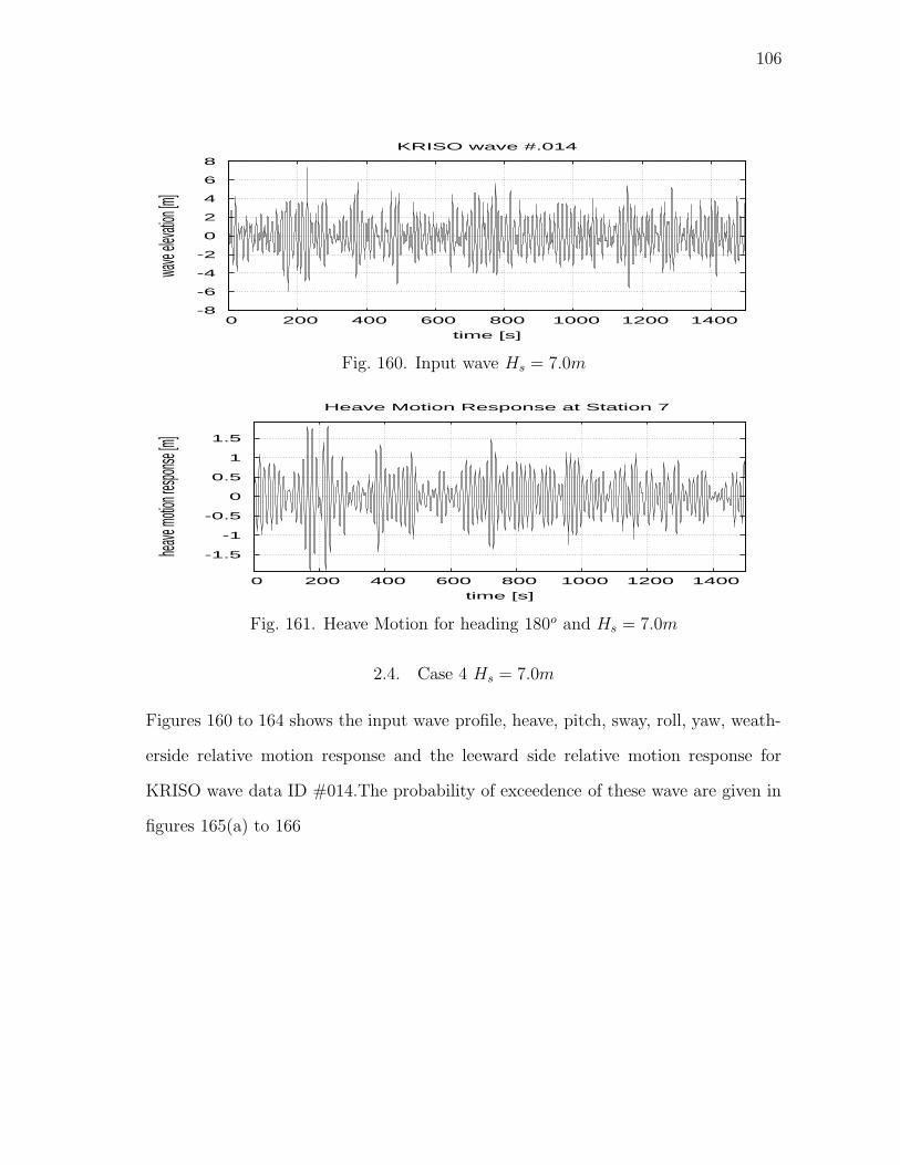
106
-8
-6
-4
-2
0
2
4
6
8
0 200 400 600 800 1000 1200 1400
wave
elevat
ion [m
]
time [s]
KRISO wave #.014
Fig. 160. Input wave Hs = 7.0m
-1.5
-1
-0.5
0
0.5
1
1.5
0 200 400 600 800 1000 1200 1400
heave
motion
respon
se [m]
time [s]
Heave Motion Response at Station 7
Fig. 161. Heave Motion for heading 180o and Hs = 7.0m
2.4. Case 4 Hs = 7.0m
Figures 160 to 164 shows the input wave profile, heave, pitch, sway, roll, yaw, weath-
erside relative motion response and the leeward side relative motion response for
KRISO wave data ID #014.The probability of exceedence of these wave are given in
figures 165(a) to 166
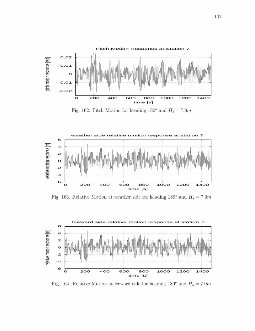
107
-0.02
-0.01
0
0.01
0.02
0 200 400 600 800 1000 1200 1400
pitch m
otion re
sponse
[rad]
time [s]
Pitch Motion Response at Station 7
Fig. 162. Pitch Motion for heading 180o and Hs = 7.0m
-6
-4
-2
0
2
4
6
0 200 400 600 800 1000 1200 1400
relative
motion
respon
se [m]
time [s]
weather side relative motion response at station 7
Fig. 163. Relative Motion at weather side for heading 180o and Hs = 7.0m
-6
-4
-2
0
2
4
6
0 200 400 600 800 1000 1200 1400
relative
motion
respon
se [m]
time [s]
leeward side relative motion response at station 7
Fig. 164. Relative Motion at leeward side for heading 180o and Hs = 7.0m
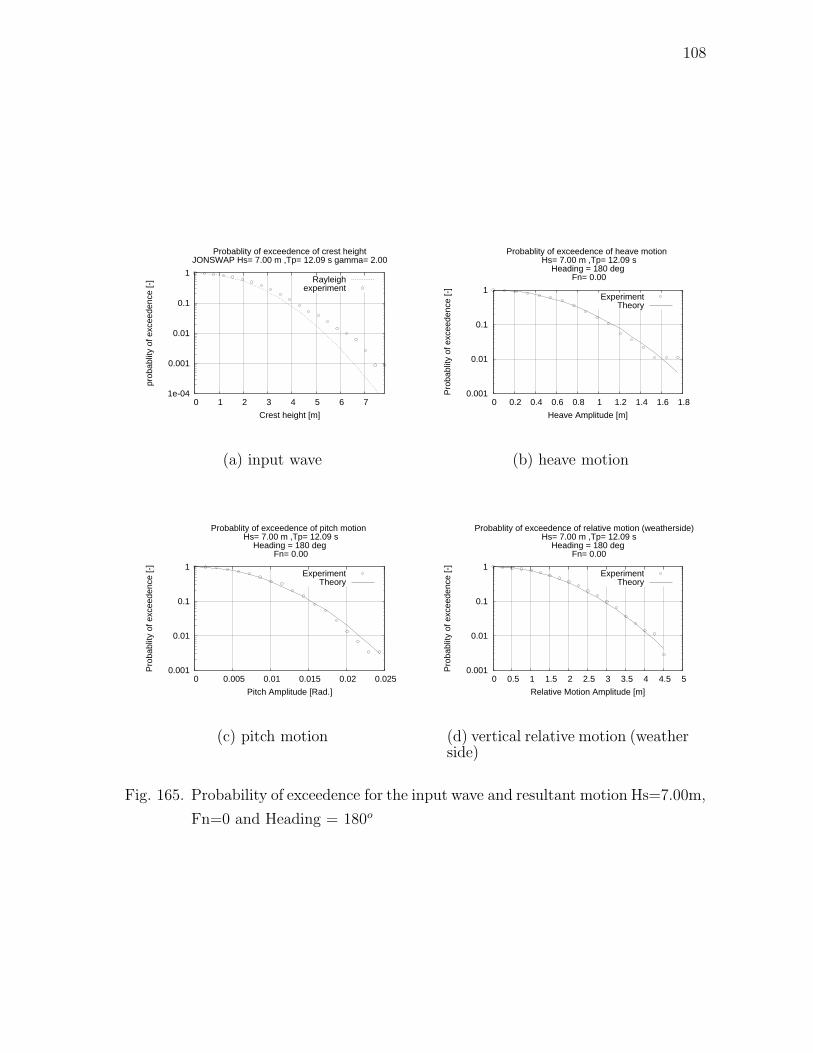
108
1e-04
0.001
0.01
0.1
1
0 1 2 3 4 5 6 7
prob
ablit
y of
exc
eede
nce
[-]
Crest height [m]
Probablity of exceedence of crest heightJONSWAP Hs= 7.00 m ,Tp= 12.09 s gamma= 2.00
Rayleighexperiment
(a) input wave
0.001
0.01
0.1
1
0 0.2 0.4 0.6 0.8 1 1.2 1.4 1.6 1.8
Pro
babl
ity o
f exc
eede
nce
[-]
Heave Amplitude [m]
Probablity of exceedence of heave motion Hs= 7.00 m ,Tp= 12.09 s
Heading = 180 deg Fn= 0.00
ExperimentTheory
(b) heave motion
0.001
0.01
0.1
1
0 0.005 0.01 0.015 0.02 0.025
Pro
babl
ity o
f exc
eede
nce
[-]
Pitch Amplitude [Rad.]
Probablity of exceedence of pitch motion Hs= 7.00 m ,Tp= 12.09 s
Heading = 180 deg Fn= 0.00
ExperimentTheory
(c) pitch motion
0.001
0.01
0.1
1
0 0.5 1 1.5 2 2.5 3 3.5 4 4.5 5
Pro
babl
ity o
f exc
eede
nce
[-]
Relative Motion Amplitude [m]
Probablity of exceedence of relative motion (weatherside) Hs= 7.00 m ,Tp= 12.09 s
Heading = 180 deg Fn= 0.00
ExperimentTheory
(d) vertical relative motion (weatherside)
Fig. 165. Probability of exceedence for the input wave and resultant motion Hs=7.00m,
Fn=0 and Heading = 180o
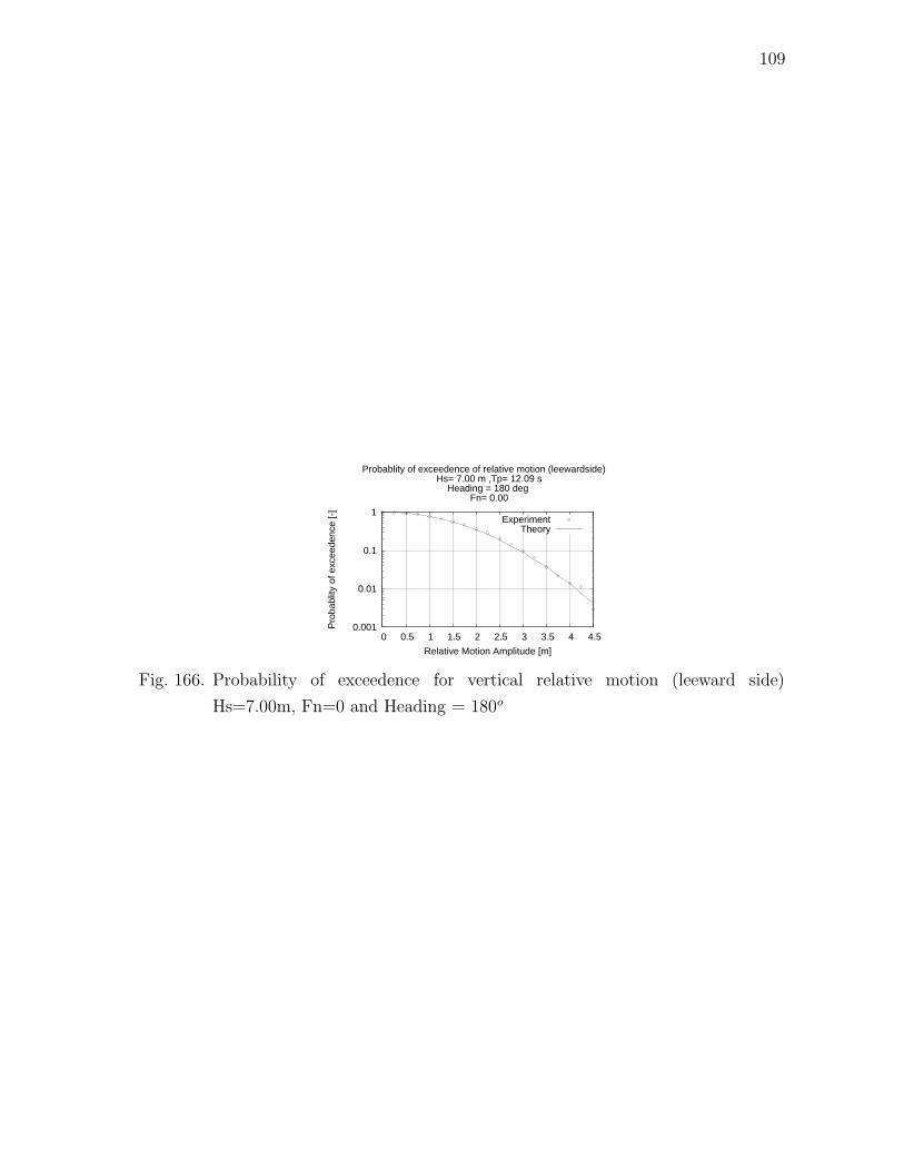
109
0.001
0.01
0.1
1
0 0.5 1 1.5 2 2.5 3 3.5 4 4.5
Pro
babl
ity o
f exc
eede
nce
[-]
Relative Motion Amplitude [m]
Probablity of exceedence of relative motion (leewardside) Hs= 7.00 m ,Tp= 12.09 s
Heading = 180 deg Fn= 0.00
ExperimentTheory
Fig. 166. Probability of exceedence for vertical relative motion (leeward side)
Hs=7.00m, Fn=0 and Heading = 180o
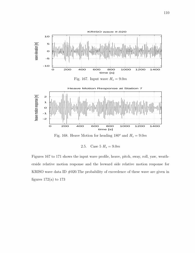
110
-10
-5
0
5
10
0 200 400 600 800 1000 1200 1400
wave
elevat
ion [m
]
time [s]
KRISO wave #.020
Fig. 167. Input wave Hs = 9.0m
-2
-1
0
1
2
0 200 400 600 800 1000 1200 1400
heave
motion
respon
se [m]
time [s]
Heave Motion Response at Station 7
Fig. 168. Heave Motion for heading 180o and Hs = 9.0m
2.5. Case 5 Hs = 9.0m
Figures 167 to 171 shows the input wave profile, heave, pitch, sway, roll, yaw, weath-
erside relative motion response and the leeward side relative motion response for
KRISO wave data ID #020.The probability of exceedence of these wave are given in
figures 172(a) to 173
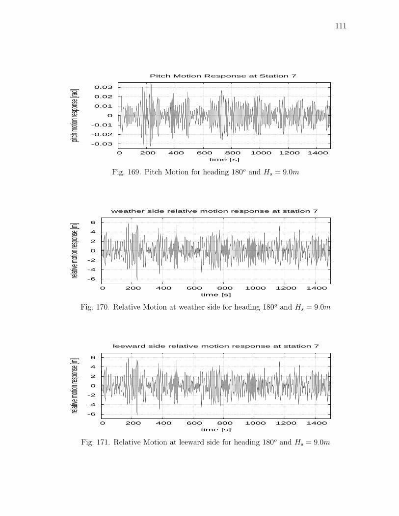
111
-0.03
-0.02
-0.01
0
0.01
0.02
0.03
0 200 400 600 800 1000 1200 1400
pitch m
otion re
sponse
[rad]
time [s]
Pitch Motion Response at Station 7
Fig. 169. Pitch Motion for heading 180o and Hs = 9.0m
-6
-4
-2
0
2
4
6
0 200 400 600 800 1000 1200 1400
relative
motion
respon
se [m]
time [s]
weather side relative motion response at station 7
Fig. 170. Relative Motion at weather side for heading 180o and Hs = 9.0m
-6
-4
-2
0
2
4
6
0 200 400 600 800 1000 1200 1400
relative
motion
respon
se [m]
time [s]
leeward side relative motion response at station 7
Fig. 171. Relative Motion at leeward side for heading 180o and Hs = 9.0m
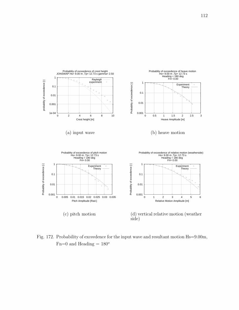
112
1e-04
0.001
0.01
0.1
1
0 2 4 6 8 10
prob
ablit
y of
exc
eede
nce
[-]
Crest height [m]
Probablity of exceedence of crest heightJONSWAP Hs= 9.00 m ,Tp= 12.73 s gamma= 2.50
Rayleighexperiment
(a) input wave
0.001
0.01
0.1
1
0 0.5 1 1.5 2 2.5 3
Pro
babl
ity o
f exc
eede
nce
[-]
Heave Amplitude [m]
Probablity of exceedence of heave motion Hs= 9.00 m ,Tp= 12.73 s
Heading = 180 deg Fn= 0.00
ExperimentTheory
(b) heave motion
0.001
0.01
0.1
1
0 0.005 0.01 0.015 0.02 0.025 0.03 0.035
Pro
babl
ity o
f exc
eede
nce
[-]
Pitch Amplitude [Rad.]
Probablity of exceedence of pitch motion Hs= 9.00 m ,Tp= 12.73 s
Heading = 180 deg Fn= 0.00
ExperimentTheory
(c) pitch motion
0.001
0.01
0.1
1
0 1 2 3 4 5 6
Pro
babl
ity o
f exc
eede
nce
[-]
Relative Motion Amplitude [m]
Probablity of exceedence of relative motion (weatherside) Hs= 9.00 m ,Tp= 12.73 s
Heading = 180 deg Fn= 0.00
ExperimentTheory
(d) vertical relative motion (weatherside)
Fig. 172. Probability of exceedence for the input wave and resultant motion Hs=9.00m,
Fn=0 and Heading = 180o
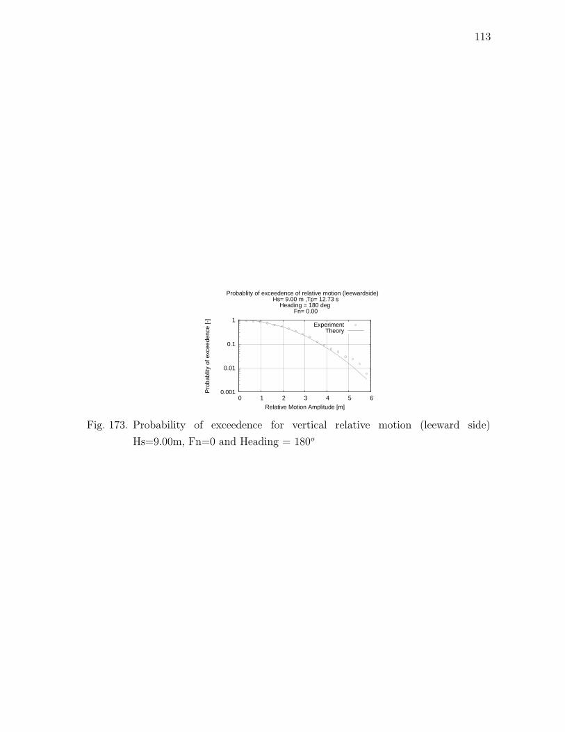
113
0.001
0.01
0.1
1
0 1 2 3 4 5 6
Pro
babl
ity o
f exc
eede
nce
[-]
Relative Motion Amplitude [m]
Probablity of exceedence of relative motion (leewardside) Hs= 9.00 m ,Tp= 12.73 s
Heading = 180 deg Fn= 0.00
ExperimentTheory
Fig. 173. Probability of exceedence for vertical relative motion (leeward side)
Hs=9.00m, Fn=0 and Heading = 180o
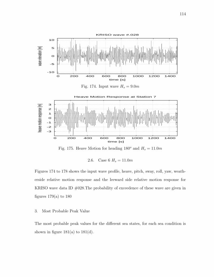
114
-10
-5
0
5
10
0 200 400 600 800 1000 1200 1400
wave
elevat
ion [m
]
time [s]
KRISO wave #.028
Fig. 174. Input wave Hs = 9.0m
-3
-2
-1
0
1
2
3
0 200 400 600 800 1000 1200 1400
heave
motion
respon
se [m]
time [s]
Heave Motion Response at Station 7
Fig. 175. Heave Motion for heading 180o and Hs = 11.0m
2.6. Case 6 Hs = 11.0m
Figures 174 to 178 shows the input wave profile, heave, pitch, sway, roll, yaw, weath-
erside relative motion response and the leeward side relative motion response for
KRISO wave data ID #028.The probability of exceedence of these wave are given in
figures 179(a) to 180
3. Most Probable Peak Value
The most probable peak values for the different sea states, for each sea condition is
shown in figure 181(a) to 181(d).
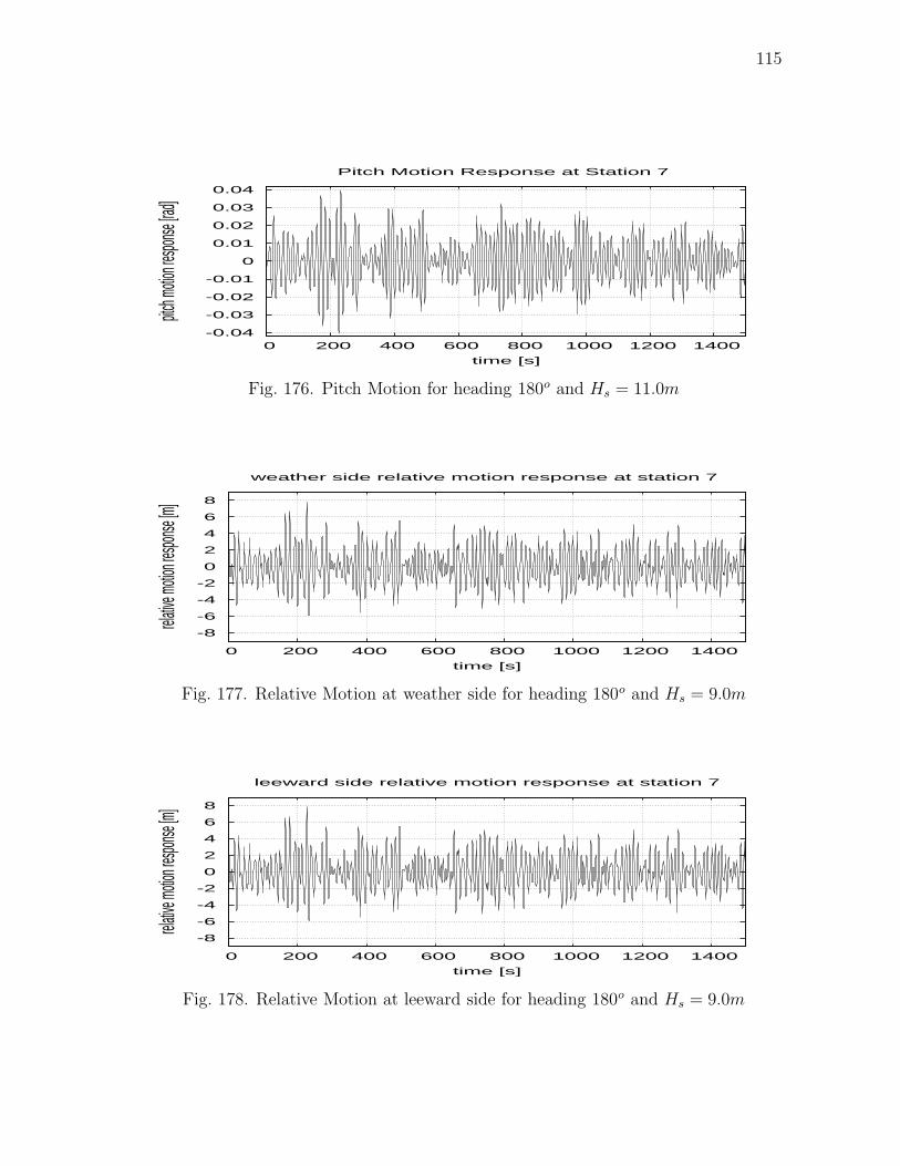
115
-0.04
-0.03
-0.02
-0.01
0
0.01
0.02
0.03
0.04
0 200 400 600 800 1000 1200 1400
pitch m
otion re
sponse
[rad]
time [s]
Pitch Motion Response at Station 7
Fig. 176. Pitch Motion for heading 180o and Hs = 11.0m
-8
-6
-4
-2
0
2
4
6
8
0 200 400 600 800 1000 1200 1400
relative
motion
respon
se [m]
time [s]
weather side relative motion response at station 7
Fig. 177. Relative Motion at weather side for heading 180o and Hs = 9.0m
-8
-6
-4
-2
0
2
4
6
8
0 200 400 600 800 1000 1200 1400
relative
motion
respon
se [m]
time [s]
leeward side relative motion response at station 7
Fig. 178. Relative Motion at leeward side for heading 180o and Hs = 9.0m
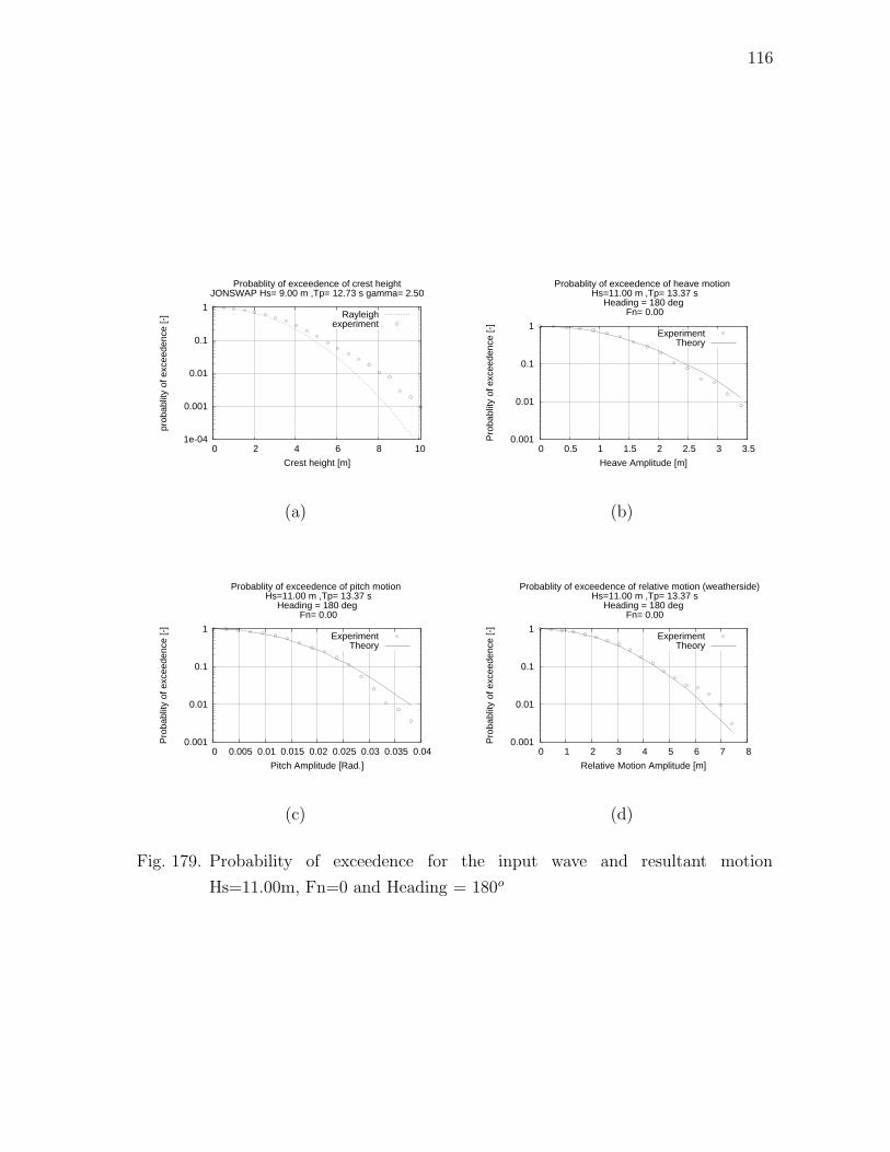
116
1e-04
0.001
0.01
0.1
1
0 2 4 6 8 10
prob
ablit
y of
exc
eede
nce
[-]
Crest height [m]
Probablity of exceedence of crest heightJONSWAP Hs= 9.00 m ,Tp= 12.73 s gamma= 2.50
Rayleighexperiment
(a)
0.001
0.01
0.1
1
0 0.5 1 1.5 2 2.5 3 3.5
Pro
babl
ity o
f exc
eede
nce
[-]
Heave Amplitude [m]
Probablity of exceedence of heave motion Hs=11.00 m ,Tp= 13.37 s
Heading = 180 deg Fn= 0.00
ExperimentTheory
(b)
0.001
0.01
0.1
1
0 0.005 0.01 0.015 0.02 0.025 0.03 0.035 0.04
Pro
babl
ity o
f exc
eede
nce
[-]
Pitch Amplitude [Rad.]
Probablity of exceedence of pitch motion Hs=11.00 m ,Tp= 13.37 s
Heading = 180 deg Fn= 0.00
ExperimentTheory
(c)
0.001
0.01
0.1
1
0 1 2 3 4 5 6 7 8
Pro
babl
ity o
f exc
eede
nce
[-]
Relative Motion Amplitude [m]
Probablity of exceedence of relative motion (weatherside) Hs=11.00 m ,Tp= 13.37 s
Heading = 180 deg Fn= 0.00
ExperimentTheory
(d)
Fig. 179. Probability of exceedence for the input wave and resultant motion
Hs=11.00m, Fn=0 and Heading = 180o

117
0.001
0.01
0.1
1
0 1 2 3 4 5 6 7 8
Pro
babl
ity o
f exc
eede
nce
[-]
Relative Motion Amplitude [m]
Probablity of exceedence of relative motion (leewardside) Hs=11.00 m ,Tp= 13.37 s
Heading = 180 deg Fn= 0.00
ExperimentTheory
Fig. 180. Probability of exceedence for the vertical relative motion (leeward side)
Hs=11.00m, Fn=0 and Heading = 180o
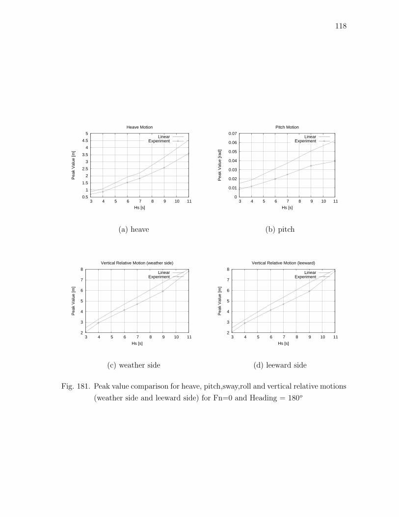
118
0.5
1
1.5
2
2.5
3
3.5
4
4.5
5
3 4 5 6 7 8 9 10 11
Pea
k V
alue
[m]
Hs [s]
Heave Motion
LinearExperiment
(a) heave
0
0.01
0.02
0.03
0.04
0.05
0.06
0.07
3 4 5 6 7 8 9 10 11
Pea
k V
alue
[rad
]
Hs [s]
Pitch Motion
LinearExperiment
(b) pitch
2
3
4
5
6
7
8
3 4 5 6 7 8 9 10 11
Pea
k V
alue
[m]
Hs [s]
Vertical Relative Motion (weather side)
LinearExperiment
(c) weather side
2
3
4
5
6
7
8
3 4 5 6 7 8 9 10 11
Pea
k V
alue
[m]
Hs [s]
Vertical Relative Motion (leeward)
LinearExperiment
(d) leeward side
Fig. 181. Peak value comparison for heave, pitch,sway,roll and vertical relative motions
(weather side and leeward side) for Fn=0 and Heading = 180o
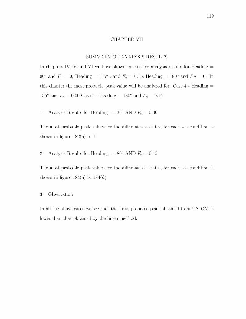
119
CHAPTER VII
SUMMARY OF ANALYSIS RESULTS
In chapters IV, V and VI we have shown exhaustive analysis results for Heading =
90o and Fn = 0, Heading = 135o , and Fn = 0.15, Heading = 180o and Fn = 0. In
this chapter the most probable peak value will be analyzed for: Case 4 - Heading =
135o and Fn = 0.00 Case 5 - Heading = 180o and Fn = 0.15
1. Analysis Results for Heading = 135o AND Fn = 0.00
The most probable peak values for the different sea states, for each sea condition is
shown in figure 182(a) to 1.
2. Analysis Results for Heading = 180o AND Fn = 0.15
The most probable peak values for the different sea states, for each sea condition is
shown in figure 184(a) to 184(d).
3. Observation
In all the above cases we see that the most probable peak obtained from UNIOM is
lower than that obtained by the linear method.
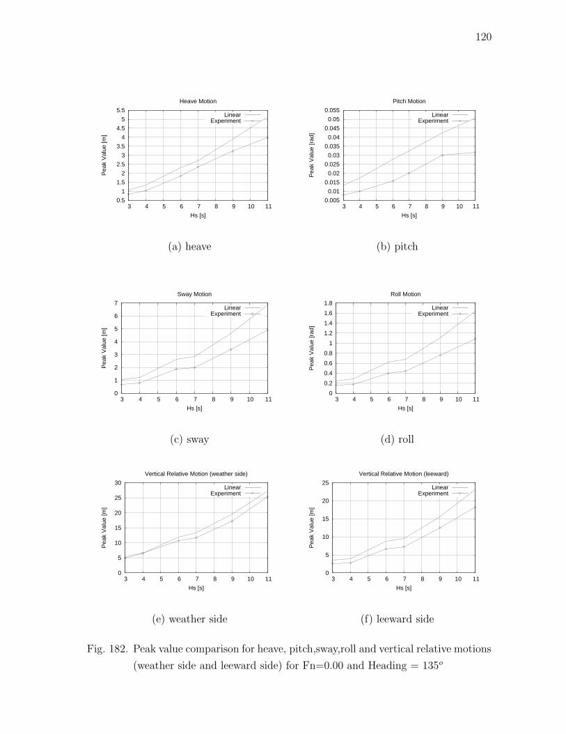
120
0.5
1
1.5
2
2.5
3
3.5
4
4.5
5
5.5
3 4 5 6 7 8 9 10 11
Pea
k V
alue
[m]
Hs [s]
Heave Motion
LinearExperiment
(a) heave
0.005
0.01
0.015
0.02
0.025
0.03
0.035
0.04
0.045
0.05
0.055
3 4 5 6 7 8 9 10 11
Pea
k V
alue
[rad
]
Hs [s]
Pitch Motion
LinearExperiment
(b) pitch
0
1
2
3
4
5
6
7
3 4 5 6 7 8 9 10 11
Pea
k V
alue
[m]
Hs [s]
Sway Motion
LinearExperiment
(c) sway
0
0.2
0.4
0.6
0.8
1
1.2
1.4
1.6
1.8
3 4 5 6 7 8 9 10 11
Pea
k V
alue
[rad
]
Hs [s]
Roll Motion
LinearExperiment
(d) roll
0
5
10
15
20
25
30
3 4 5 6 7 8 9 10 11
Pea
k V
alue
[m]
Hs [s]
Vertical Relative Motion (weather side)
LinearExperiment
(e) weather side
0
5
10
15
20
25
3 4 5 6 7 8 9 10 11
Pea
k V
alue
[m]
Hs [s]
Vertical Relative Motion (leeward)
LinearExperiment
(f) leeward side
Fig. 182. Peak value comparison for heave, pitch,sway,roll and vertical relative motions
(weather side and leeward side) for Fn=0.00 and Heading = 135o
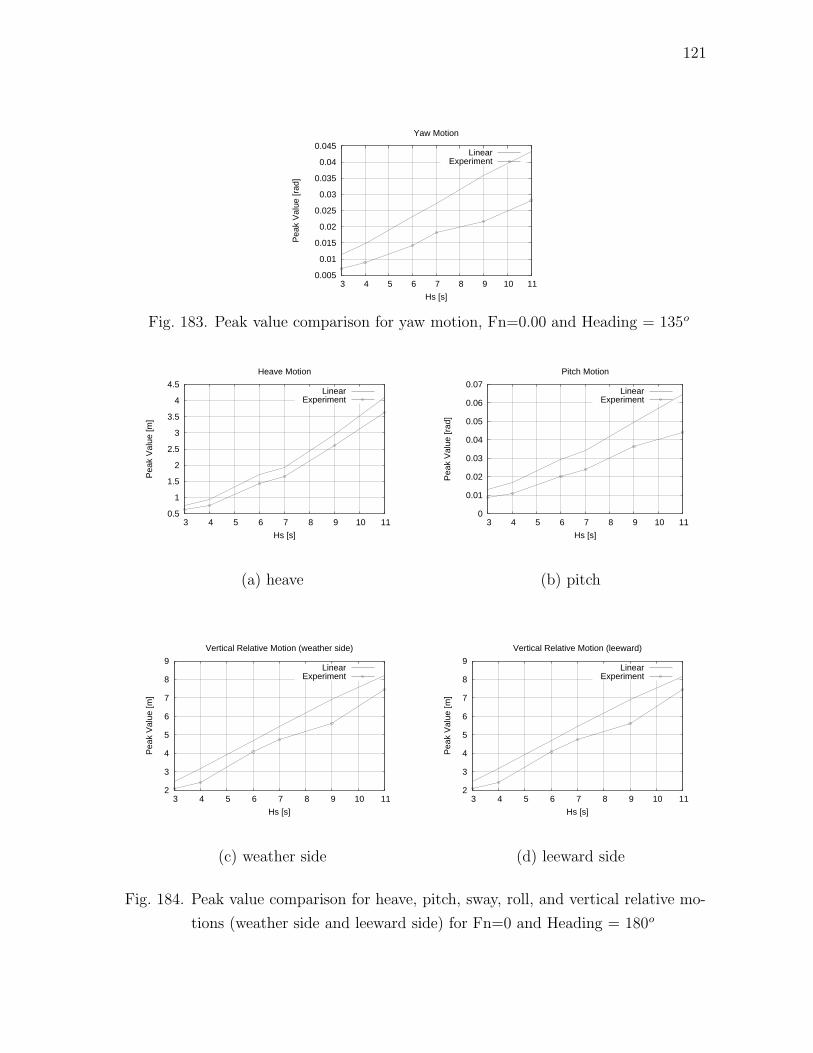
121
0.005
0.01
0.015
0.02
0.025
0.03
0.035
0.04
0.045
3 4 5 6 7 8 9 10 11P
eak
Val
ue [r
ad]
Hs [s]
Yaw Motion
LinearExperiment
Fig. 183. Peak value comparison for yaw motion, Fn=0.00 and Heading = 135o
0.5
1
1.5
2
2.5
3
3.5
4
4.5
3 4 5 6 7 8 9 10 11
Pea
k V
alue
[m]
Hs [s]
Heave Motion
LinearExperiment
(a) heave
0
0.01
0.02
0.03
0.04
0.05
0.06
0.07
3 4 5 6 7 8 9 10 11
Pea
k V
alue
[rad
]
Hs [s]
Pitch Motion
LinearExperiment
(b) pitch
2
3
4
5
6
7
8
9
3 4 5 6 7 8 9 10 11
Pea
k V
alue
[m]
Hs [s]
Vertical Relative Motion (weather side)
LinearExperiment
(c) weather side
2
3
4
5
6
7
8
9
3 4 5 6 7 8 9 10 11
Pea
k V
alue
[m]
Hs [s]
Vertical Relative Motion (leeward)
LinearExperiment
(d) leeward side
Fig. 184. Peak value comparison for heave, pitch, sway, roll, and vertical relative mo-
tions (weather side and leeward side) for Fn=0 and Heading = 180o
122
CHAPTER VIII
CONCLUSION
Conventionally the responses of the ship to different sea states are calculated in the
frequency domain using the linear theory. This method is prone to over-predictions
for nonlinear waves. The linear approach is based on the assumption that the process
is a narrow band Gaussian process. This explains why the predictions are different
from the simulated values.
The study shows the validity of the UNIOM approach over the linear theory. The
probability of exceedence study has shown that the responses are actually lower than
those calculated using the spectral approach, thus being in line with the experiments
done by Dalzell (Cummins 1973). This confirms the validity of the UNIOM approach
in calculating the responses of a floating body in an irregular seaway.
The predictions using the linear method and UNIOM match closely for the lower
sea states, this is apparent in figure 137(e). In this figure at low sea states, the values
predicted by UNIOM overshoots the value predicted by the linear theory. However,
at higher sea states there is marked difference in this and the linear theory is seen to
over predict.
This trend is attributed to the fact that the lower sea states are more close to
being linear whereas the higher sea states show marked nonlinear behavior. Therefore,
the higher sea states show greater divsersions from the linear predictions.
Thus UNIOM seems to be applicable to predict non linear effects on vertical
relative motion and other modes as well. It is hoped that this method may be
developed further to be more generic. However to quantitatively conclude that this
method explains the non linearity of ship motions, we require experimental data.
In the future, UNIOM can be applied to a ship sea-way system, using the

123
Quadratic Transfer Function (QTF) in place of the RAO. This will represent the
nonlinearities in ship responses more accurately.
124
REFERENCES
Adil, A. 2004 Simulation of ship motion and deck-wetting due to steep random
sea. Masters thesis, Texas A&M University, College Station, Texas.
Bhattacharyya, R. 1978 Dynamics of Marine Vehicles. John Wiley and Sons,
New York.
Chakrabarti, S. K. 1994 Offshore Structure Modeling. World Scientific, River
Edge, NJ.
Cummins, W. 1973 Pathologies of the transfer function. Report. Naval Ship
Research and Development Center, Bethesda, Maryland.
Dalzell, J. 1982 An investigation of the applicability of the third degree functional
polynomial model to non-linear ship motion problem. Report SIT-DL-82-9-2275.
Stevens Institute of Technology, Hoboken, NJ.
Dean, R. G. and Dalrymple, R. A. 1984 Water Wave Mechanics for Engineers
and Scientists. World Scientific, River Edge, NJ.
Journee, J. and Massie, W. 2001 Offshore Hydrodynamics. located at
www.shipmotions.nl and accessed on March 2006.
Kim, C. H. 2006 Non Linear Waves and Offshore Structures. World Scientific,
River Edge, NJ.
Kim, C. H., Chou, F. S. and Tein, D. 1980 Motions and hydrodynamic loads
of a ship advancing in oblique waves. Trans. SNAME, 88, 1, Mar, 29.
Richer, J. 2005 The effects of wave groups on the nonlinear simulation of ship
motion in random sea. Masters thesis, Texas A&M University, College Station,
Texas.
125
VITA
ADDRESS
Room # 202, Ocean Engg Division,
Dept. of Civil Engg,
Texas A&M University,
College Station,
TX-77843-3136.
EDUCATION
Master of Science in Ocean Engineering. Graduation Date: May 2006
Major : Ocean Engineering
(August 2004 - May 2006)
Texas A&M University
Bachelor of Technology in Naval Architecture and Ship Building
Major : Naval Architecture and Ship Building
(September 1997 - May 2002)
Cochin University of Science and Technology,
Cochin, Kerala, India.
EXPERIENCE Graduate Teaching assistant with the Ocean Engineering program
(2005 - 2006) Naval Architect - A B Marine Consultants (2002 November - 2004
August)
The typist for this thesis was Rajith Padmanabhan.