Experiments : design, parametric and nonparametricanalysis, and selectionvan der Laan, P.

Published: 01/01/1992

Document VersionPublisher’s PDF, also known as Version of Record (includes final page, issue and volume numbers)

Please check the document version of this publication:

• A submitted manuscript is the author's version of the article upon submission and before peer-review. There can be important differencesbetween the submitted version and the official published version of record. People interested in the research are advised to contact theauthor for the final version of the publication, or visit the DOI to the publisher's website.• The final author version and the galley proof are versions of the publication after peer review.• The final published version features the final layout of the paper including the volume, issue and page numbers.

Link to publication

Citation for published version (APA):Laan, van der, P. (1992). Experiments : design, parametric and nonparametric analysis, and selection.(Memorandum COSOR; Vol. 9215). Eindhoven: Technische Universiteit Eindhoven.

General rightsCopyright and moral rights for the publications made accessible in the public portal are retained by the authors and/or other copyright ownersand it is a condition of accessing publications that users recognise and abide by the legal requirements associated with these rights.

• Users may download and print one copy of any publication from the public portal for the purpose of private study or research. • You may not further distribute the material or use it for any profit-making activity or commercial gain • You may freely distribute the URL identifying the publication in the public portal ?

Take down policyIf you believe that this document breaches copyright please contact us providing details, and we will remove access to the work immediatelyand investigate your claim.

Download date: 22. Jun. 2018

EINDHOVEN UNIVERSITY OF TECHNOLOGYDepartment of Mathematics and Computing Science

Memorandum COSOR 92-15

Experiments: Design, Parametric andNonparametric Analysis, and Selection

P. van der Laan

Eindhoven, June 1992The Netherlands

Eindhoven University of TechnologyDepartment of Mathematics and Computing ScienceProbability theory, statistics, operations research and systems theoryP.O. Box 5135600 MB Eindhoven - The Netherlands

Secretariate: Dommelbuilding 0.03Telephone: 040-47 3130

ISSN 0926 4493

Experiments: Design, Parametric and N onparametric

Analysis, and Selection

Paul van der LaanEindhoven University of Technology

Department of Mathematics and Computing ScienceEindhoven, The Netherlands

SummarySome general remarks for experimental designs are made. The general statistical methodologyof analysis for some special designs is considered. Statistical tests for some specific designsunder Normality assumption are indicated. Moreover, nonparametric statistical analysesfor some special designs are given. The method of determining the number of observationsneeded in an experiment is considered in the Normal as well as in the nonparametric situation.Finally, the special topic of designing an experiment in order to select the best out of k(? 2)treatments is considered.

Experiments: Design, Parametric and Nonparametric

Analysis, and Selection

Contents

1. Introduction

2. General remarks

3. Special designs

4. The number of observations: Normal distribution

5. The number of observations: Xonparametric situation

6. Analysis of variance and nonparametric analysis of some specific designs

7. Design and analysis of selection experiments

8. Final remarks

Literature

1

4

7

14

22

30

40

4.5

46

1. Introduction

In various fields of industrial investigation or biological and agricultural research the ob­servational data are of a variable nature. Even when the conditions of an experiment arekept constant as much as possible the outcome or response variable will vary from one trialto another. This variability is indicated by the term:

experimental error

or error. A perfect repetition of a treatment to experimental units is in practice impossible.There is always some variation in the effect of the same treatment applied to different exper­imental units. This difference is due to heterogeneity of the material, errors of observation,but also the failure to repeat the treatment exactly. Division of the material and allocation tothe different treatments in a random way is therefore of essential importance. A completelyrandomized design is a plan for collecting data in which a random sample is selected fromeach treatment, and the samples are normally supposed to be independent.However, this kind of error is often only a small part of the variability. The main reasons forvariability are often uncontrolled instruments or environmental factors like

temperature

humidity

pressure

pollution

etc. Statistical designs of experiments and corresponding statistical parametric or nonpara­metric methods of analysis cal~ help us to draw conclusions from data with random fluctua­tions.In order to achieve that the variability is of a random nature a good design is important.Replication and randomization are, besides the use of blocks, two principal aspects of design­ing an experiment. Often the responses in an experiment are subject to sources of variationin addition to the treatments under study. Suppose for instance that in a field experiment aresearch worker is studying the yield resulting from four varieties of wheat. If the experimen­tal area is divided into a number of smaller areas of equal size, the blocks or replications, andeach of these blocks are divided into a number of plots (units), then randomization withineach block is carried out and we have in this case a so-called 'randomized block design'. Arandomized block design is a plan for collecting data in which each of k treatments is mea­sured once in each of b blocks. The order of the treatments within the blocks is random.In this report general concepts and ideas of statistical aspects of experimental designs areconsidered and discussed. A good design of an industrial or scientific experiment is essentialfor correct and efficient investigation. A correct design makes it possible to draw correct andjustified conclusions.For answering questions data have to be collected from experimental units. For industrialexperiments machines, ovens and other similar objects form experimental units. For agricul­tural experiments equal sized plots of land, a single or a group of plants, a single or a groupof animals are used as experimental units.

1

About sixty years ago the main principles of experimental design were formulated at Rotham­sted Experimental Station in United Kingdom. The pioneer in this field was Ronald A. Fisher.He published the results in his book 'The Design of Experiments' in 1935. In 1966 the 8-thedition appeared. During the period after the appearance of Fisher's book on experimentaldesign an impressive stream of papers and books dealing with design of experiments and thecorresponding parametric and nonparametric statistical analysis have been published. Thecorresponding parametric analysis is indicated by the name 'analysis of variance'. Why do wefind so many uses of statistics in the analysis of a design? Because many of the decisions wemake are based on uncertain data. Moreover, there is a need for greater efficiency. Finally,there is also a need for more complex experiments. Not only one factor is of interest, oftena large number of factors and their possible interactions are important and have possiblyinfluence on the response variable. Most people are poor at measuring and distinguishingbetween large number of factors. A statistical design in which the factors can simultaneouslybe varied is of great importance. Statistics is not just a set of techniques, it is an attitudeof mind in approaching data. In particular it acknowledges the uncertainty and variabilityin data and data collection. Statistics is making decisions in the face of this uncertainty.Designing experiments in a statistically sound way and the corresponding parametric or non­parametric statistical analysis are of vital importance for good decision making.Before collecting data and analysing these data it is important to give careful thought to theproper design of an experiment. A project has in general three phases:

the experiment

the design

the analysis.

A first question is: 'What is the goal of the experiment?' The experiment includes a state­ment of the problem to be solved.The purpose of an experiment is the responsibility of the research worker, not of the statis­tician. The research worker has to answer the question: 'What is he going to do with theresults of the experiment?'It is necessary to define the dependent or response variable and the independent variablesor factors which may affect the response variable. Are the factors qualitative or quantita­tive? Can they held constant? Are the levels of the factors certain fixed values or are theya random choice from a population of all possible levels? Experimentation, designing a goodexperiment and an adequate statistical inference are essential features of general scientificand industrial methodology. A proper design, such that the interpretation of the data canbe done in a valid way, is essential.There are many books written on designing experiments. To mention a few: Kempthorne(1952), Cochran and Cox (1957), Federer (1955), Montgomery (1984), Cox (1966). The lastmentioned book is well-known and is mainly dealing the fundamental concepts of with de­signing an experiment. It can be seen as a basic guide-line for experiments design. The otherbooks are mainly dealing with the analysis of experiments.It is the purpose of the next chapter of this report to present the fundamental concepts in thedesign of experiments. In later chapters also the analysis will be indicated. Chapter 3 is deal­ing with special designs as Incomplete Block Designs and Fractional replication. Chapter 4 isdealing with the required number of observations under the Normality assumption, whereas

2

Chapter 5 presents a nonparametric approach. Chapter 6 gives an analysis, parametric andnonparametric, of a number of problems. Chapter 7 presents the selection problem: designand analysis. Finally, in Chapter 8 a number of remarks are made.

3

2. General remarks

In this chapter we shall describe general concepts and general designs as Randomized Blocks,Latin Squares and Factorial Designs.Large uncontrolled variation is common in biological sciences. For this reason effects of treat­ments under investigation are often masked by fluctuations outside the experimenter's controland the designing of experiments is an essential part of scientific research in order to makeit possible to draw valid conclusions in an efficient way.Let us take the following example. In an agricultural experiment one wants to compare differ­ent varieties (treatments in general). The experimental area is divided into plots of equal size(experimental units or units in general) and the varieties are assigned randomly to the plots.In general, neighbouring plots tend to give yield more alike than distant plots. It is possiblethat there is a systematic variation across the field. A different year or a different field mayproduce substantial different results. The uncontrolled variation is often large compared withthe treatment effects. It is essential in most cases (or always (!» to plan a good experimentin order to detect differences in treatment effects while so much variation associated with theexperimental units is present.For a good experiment it is required that the experimental units receiving treatment Tl differin no systematic way from the experimental units receiving treatment T2 • In this way it ispossible to estimate the true treatment effect of Tl minus T2 without a systematic error. Inthis context the key word is

randomization.

Randomization makes it possible that possible differences in experimental units are randomlydivided to the treatments. The influence of this error is measured by the so-called standarderror. It is the magnitude of the random errors in the estimate of the treatment contrast.In fact, the standard error of the difference between two treatments Tl and T2 is equal to(T(n!l + n2"l)t, where ni is the number of observations (experimental units) of Ti(i = 1,2).The standard error tends to zero if 111 and 112 tend to infinity. The number of experimentalunits is important in order to get a sufficiently small standard error. However, too manyunits has a disadvantage that small treatment effects may be detected, which are generallyof no practical importance. Then the investment in time and energy was too large.From a practical point of view an important remark is that the whole experiment mustbe relatively simple. The reason is the fact that in most cases the experiment has to becarried out by unexperienced people, unexperienced in statistical principles and thereforenot conscious of the importance of a statistically correct execution of the experiment. Forinstance the fact that randomization is of vital importance, is not always realized.We assume that the treatment effects add on to the experimental unit term and that theeffect of a treatment is constant during the whole experiment.Usually, when the numbers of units for treatments T1 and T2 are equal, the difference betweenT1 and T2 is estimated by the difference of the means of all observations on T1 and T2 ,

respectively.Moreover, it is of course not allowed that an experimental unit is affected by the treatmentapplied to the other experimental units. In other words, it is supposed that there is nointerference between different experimental units. One has to be careful when an experimentalunit is used different times (overflow effect), or if different experimental units are in physicalor psychological contact (dependency). In agricultural experiments guard rows are left out of

4

consideration. In psychological experiments using a person several times, it is possible thatthe response is dependent on the whole sequence of situations that have preceded it.The precision (or standard error) can be improved by taking more experimental units. Analternative is to improve the design of the experiments. This aspect can be illustrated by asimple (but practically important) situation, namely the comparison of just two treatmentsT1 and T2 • The main aspect of this situation will be the design. The statistical analysis ofthe data is closely related to the design. That's the reason we shall also give the analysis.Using this situation we shall discuss the three basic principles of experimental design, namely

replication

- randomization

blocking

Replication is the repetition of the basic experiment. It provides an estimate of the experi­mental error. Then it is possiule to investigate a possible statistical significance of a differencein treatments. If 0'2 is the variance of the data and there are n replicates, then the varianceof the sample mean is O'f = "': ' so a more precise estimate of the mean of Y is possible. Ingeneral: More replications increase the accuracy of estimates of the treatment effects or morereplications result in more accurate conclusions. If a treatment is allocated to r experimentalunits in an experiment, it is said to be replicated r times (not: r - 1). If in a design each ofthe treatments is replicated r times, the design is said to have r replications.

Randomization is of vital importance. Statistical methods require that the observationsor eITors are independently distributed. Randomization usually makes this assumption cor­rect. By randomization we mean that the allocation of the experimental material as well asthe order in which the individual runs or trials of the experiment are to be performed arerandomly performed. See also the instructive Example 5.9 in Cox (1966).By proper randomization, the effects of possible extraneous factors will also be averaged out.This aspect can easily be illustrated in the example to be given for the comparison of twotreatments.The randomization of treatments can be realized as follows. Random numbers are drawn withthe aid of a table with random digits (random tables) or computer. For t treatments we needat random numbers, where a equals the number of times a treatment occurs in the wholeexperiment (or in a part of the experiment). Ranking the random numbers in increasingorder, produces a random permutation of the treatments. It is clear that for each experimentwe need new random digits. Using the same random digits for different experiments is a verybad attitude.To use a systematic pattern is also very dangerous. The same order (Tl, T2 ) for each blockcan be totally wrong. For instance, when T1 and T2 are measured after each other and a dif­ference in time has influence. Also a system of ordering (Tll T2 ), (T2 , T1 ), (Tll T2 ), (T2 , T1 ), ...

can be very dangerous, when this pattern coincides with some pattern in the uncontrolledvariation in an agricultural field experiment.As a conclusion, we can formulate that randomization makes it possible that unbiased esti­mates of the treatment effects, unbiased estimate of the error variance, and exact significancetests concerning the treatment effects can be obtained.Blocking is a cornerstone of experimental design. It provides a method in order to increase

5

the precision of an experiment, or more precisely a larger precision with the same number ofobservations. Reducing the error can be done by making experimental units homogeneous.This can be achieved by forming the experimental units into several homogeneous groups,usually called blocks, allowing variation between the blocks. A block is a portion of theexperimental material that is more homogeneous than the whole collection of material.All these aspects can be illustrated in the next example of the comparison of just two treat­ments T1 and T2 •

If there are 20 experimental units, then 10 units can be randomly allocated to T1 and therest to T2 • The effect of this uncontrolled variation on the error of the treatment comparisoncan be reduced by obtaining pairs of units as alike as possible. We suppose that there is nosystematic difference between the first and the second unit in a pair. The two units in a pairare expected to give as nearly as possible identical observations in the absence of treatmentdifferences. The correct procedure is to randomize the order of T1 and T2, independently foreach pair. The succes of 'paired comparisons' depends on an efficient pairing of the units.

6

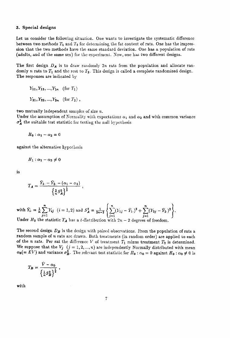
3. Special designs

Let us consider the following situation. One wants to investigate the systematic differencebetween two methods T1 and T2 for determining the fat content of rats. One has the impres­sion that the two methods have the same standard deviation. One has a population of rats(adults, and of the same sex) for the experiment. Now, one has two different designs.

The first design DAis to draw randomly 2n rats from the population and allocate ran­domly n rats to T1 and the rest to T2 • This design is called a complete randomized design.The responses are indicated by

Yn , Y12, ... ,Y1n (for TI)

two mutually independent samples of size n.Under the assumption of Normality wit.h expectations 0:1 and 0:2 and with common varianceO'~ the suitable test statistic for testing the null hypothesis

against the alternative hypothesis

1S

n { n n }with fi. = ~ L:l'ij (i = 1,2) and 51 = 2n1_2 L:(Y1j - Yd2+L:(Y2j - Y2.)2 .;=1 j=l ;=1

Under Ho the statistic TA has a i-distribution with 2n - 2 degrees of freedom.

The second design DB is the design with paired observations. From the population of rats arandom sample of n rats are drawn. Both treatments (in random order) are applied to eachof the n rats. Per rat the difference V of treatment T1 minus treatment T2 is determined.We suppose that the Vj (j = 1,2, ... , n) are independently Normally distributed with meanQo(= EV) and variance 0'1. The relevant test statistic for Ho : 0:0 = 0 against H o : Qo i= 0 is

with

7

2 1 ~ - 25B = -- L.,,(Vj - 11) .n - 1 j=1

The test statistic TB has under JIo a t-distribution with n - 1 degrees of freedom.The numerators of both test statistics are of equal merit, for ao = al - a2 and applicationof the prescription if to the 217, observations will give the same result as the prescription¥t. - Y2 ..But the denominators are totally different.For the design DA, the complete randomized design, there are two components in the vari­ability of fat contents:

error of measurement

variability of fat content of the rats.

For the design DB, with paired observations, only the error of measurement is present. Bytaking differences the influence of fat content has been eliminated.Suppose the variance of the error of measurements is O"~, then ~5~ has expectation ~0"1 =~20"~ for difference has variance O"~ + O"~ = 20"~. For design DA the denominator (besidesthe square root) ~5~ has expectation ~O"~ = ~(O"~ + O"~), with O"~ the variance of the ratpopulation.We have

2 2-(0"2 + 0"2) > _0"2 if and only if O"p2 > 0 .n m p n m

From this it follows that under the alternative hypothesis using DB the null hypothesis willbe rejected sooner than using DA. The influence of the difference in critical values (for 2n - 2and 2n degrees of freedom) is not so important.For the two designs D A and DB the confidence intervals for al - a2 with confidence level0.95 have expected midpoints al - 02 == 00 and lengths

{2 2}~

LA = 2t2n-2jO.975 ;,5A

and

{I 2}}

LB = 2tn -ljO.975 ;,5B ,

respectively, with P(Tm :::; tmjl-oy) = 1 - ')', where Tm has a t-distribution with m degrees offreedom. In general, 25~ >> 5~ and the difference between t2n-2jO.975 and t n - 1jO.975 is notso large, which is illustrated in next table.

8

n t2n-2;0.975 tn -1jO.975

2 4.303 12.7063 2.776 4.3034 2.447 3.1825 2.306 2.776

10 2.101 2.26220 2.025 2.09330 2.002 2.04540 1.994 2.02300 1.960 1.960

If 81 > 51 then DAis less efficient than DB for n > 2. Certainly, for n ~ 5 or 10 thedifference between the critical values becomes rather small.

ExampleUsing design DB the following numerical results are given

Treatment Diff.1 2 v

15.4 16.1 -0.715.4 16.5 -0.115.9 15.5 0.416.7 17.6 -0.916.0 17.6 -1.617.4 18.5 -1.117.2 17.9 -0.717.3 18.3 -1.015.5 17.9 -2.416.0 16.0 0.0

From the results it follows th'lt

v = -0.81

10

l)Vj - v)2 = 5.929 ,;=1

thus

2 5.929sB = -- = 0.659 .

9

We get for testing Ho : ao = 0 the test statistic

-0.81tB = = -3.155

y'0.659!1O

9

and Ho is rejected, because t9;0.975 = 2.262 and thus t9;0.025 = -2.262. An estimate for O'~ isequal to 0.~59 = 0.330.Now we can estimate O'~ as if the observations have been obtained using design DA. Thestatistics ~(Yli - fi.)2 and ~(Y2j_1T2.)2 are now stochastically dependent (for Y1i and Y2j arebelonging to the same rat), but the expectation of both sums is 90'~. The unbiased estimateof O'~ is equal to

{8 {2836.33 - (162.8)2 j10 +2965.19 - (171.9)2 j10} = 1.349 .

Thus an estimate of O'~ is equal to

1.349 - 0.330 = 1.019 .

From this it follows that ('y = .05):

DA DBo-m = .574 o-m = .574o-p = 1.0000-A = 1.1G1 GB = .812LA = 2 * 2.101 * .519 LB = 2 *2.262 * .257= 2.18 = 1.16'ConLint.' ConLint.(-1.90, .28) (-1.39, -.23)

Substitution in tA should give 1.850 with probability of exceedance less than .10 assumingthe t-distribution holds (which is not true).

An interesting question is 'What number of observations for D A leads to the same length ofthe confidence interval?' The requirement is (neglecting the difference in critical values):

2S~ 2 * 1.349-2 = =4.09SB 0.659

as many observations for DA. Thus 10 rats for DB and 2 *40 = 80 rats for DA. The relativeefficiency of DA (relative with respect to DB) is estimated by ~g = l.

Randomized BlocksA natural generalization of paired comparisons is to consider the situation with t(> 2) treat­ments. If there are t treatments we can make blocks of size t. The units in each block areexpected to give as nearly as possible the same observations if the treatments are equivalent(in their effect). The order of treatments is randomized within each block. Each treatmentoccurs once in each block and the randomizations for the blocks are independent. The compar­ison of the treatments will take place within blocks, so the effect of variations between blocksis eliminated, so far as treatment comparisons are concerned. The general idea of groupingis frequently used in simple experiments as well in more complicated designs. As comparisonof treatments takes place within blocks and the effect of constant differences between blocks

10

is eliminated, a good grouping of experimental units into block is of fundamental importance.

Latin Squares and Graeco-Latin SquaresA natural extension of the randomized block design is the Latin Square. In the randomizedblock design there is one system of grouping. It might happen that there are systematicdifferences between the units within blocks. Then we should have two sytems of grouping,into blocks and into order within blocks. We would wish to balance out both systematicvariations. A restriction which limits the use of Latin Squares is that the number of blocks(rows) and the number of experimental units in a block (columns) are equal. Assume thisnumber is equal to k. Then a Latin Square is a design in which k2 units are divided in threeways into k classes of k elements, such that the divisions are pairwise orthogonal (propor­tional representation). In each row and each column each treatment is present once and onlyonce.The following example has three treatments indicated with the Latin characters A, BandC (e.g. industrial processes). There are two kinds of blocking: one corresponding with rows(e.g. Location) and one corresponding with columns (e.g. Days).

Day123

1Location 2

3

A B CB C AC A B

The Latin Square can be used when the experimental units are simultaneously grouped intwo ways. If the experimental units are grouped in three ways, then a Graeco-Latin Squareis suitable. For k = 3 we have

Day1 2 3

1 A,a B,(3 C,'YLocation 2 C,(3 A,'Y B,a

3 B,'Y C,a A,(3

For example: The Latin characters A, Band C correspond with observers and the Greekcharacters a, f3 and 'Y correspond with three industrial processes. Each observer measuresonly one process on each day. The Greek characters are situated such that each observeroccurs once in combination with each industrial process, whereas each observer measuresonce in each day and once at each location.For both kinds of squares the arrangement of treatments (persons, processes, locations, days)should be determined by randomization.

Concomitant observationsIn order to reduce error or to increase precision not only grouping into blocks can be used, butalso the use of concomitant or supplementary observations. Then with each main observationfor which we try to find the treatment effects, for each experimental unit we have one (ormore) concomitant observations. The condition is that the value for any unit must be unaf­fected by the particular assignment of treatments to units actually used. This can be realized

11

by observing the concomitant variable before the treatment is applied, or before the effect ofthe treatment has had time to develop. Examples of concomitant variables are the yield ofa variety of wheat on a plot in previous years, or the weight of the heart of an experimentalanimal use in a biological assay. Also the weight at the start of a diet experiment may beimportant for an efficient analysis. The proper technique of analysis for such an experiment isthe analysis of covariance. For a simple model it is often possible to find the effects graphically.

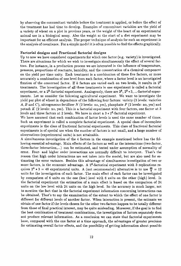
Factorial designs and Fractional factorial designsUp to now we have considered experiments for which one factor (e.g. variety) is investigated.There are situations for which we wish to investigate simultaneously the effect of several fac­tors. For instance, in a production process we are interested in the influence of temperature,pressure, proportions of reactants, humidity, and the concentration of a chemical componenton the yield per time unity. Each treatment is a combination of these five factors, or moreaccurately a combination of one level from each factor, where a factor level is an investigatedfixation of the concerned factor. If k factors are varied each on two levels, it results in 2le

treatments. The investigation of all these treatments in one experiment is called a factorialexperiment, or a 2le-factorial experiment. Analogously, there are 3le , 23 *3, ...-factorial exper­iments. Let us consider the following agricultural experiment. We want to investigate theyield per plot of wheat in dependence of the following four factors: variety (3 levels: varietiesA, B and C), nitrogeneous fertilizer N (2 levels: no, yes), phosphate P (2 levels: no, yes) andpotash J( (2 levels: no, yes). This is a factorial experiment with four factors, one factor at 3levels and three factors at 2 levels. We have in short a 3 *23-factorial experiment.\Ve have assumed that each combination of factor levels is used the same number of times.Such an experiment is called a complete factorial experiment. A special class of incompleteexperiments is the class of fractional factorial experiments. This class of fractional factorialexperiments is of special use when the number of factors is not small, and a large number ofobservations (experimental units) is not attainable.A simultaneous investigation of the 4 factors in the example mentioned before has the fol­lowing essential advantage. Main effects of the factors as well as the interactions (two-factor,three-factor interaction,... ) can be estimated, and tested under assumption of normality oferror. Four- and higher order interactions are normally difficult to interpret. That's thereason that high order interactions are not taken into the model, but are also used for es­timating the error variance. Besides this advantage of simultaneous investigation of two ormore factors, is the economic advantage. A 24-factorical experiment with 3 replications re­quires 24 * 3 == 48 experimental units. A (not recommended) alternative is to use ~ = 12units for the investigation of each factor. The main effect of each factor can be investigatedby comparison of 6 units on the one (low) level with 6 units on the other (high) level. Inthe factorial experiment the estimation of a main effect is based on the comparison of 24units on the low level with 24 units on the high level. So the accuracy is much larger, notto mention the fact that in the factorial experiment information concerning interactions canbe obtained. That's to say the examination of the extent to which the effect of one factor isdifferent for different levels of another factor. When interaction is present, the estimate weobtain of one factor if the levels chosen for the other two factors happen to be totally differentfrom those of final practical interest, may be quite misleading. Moreover, if the goal is to findthe best combination of treatment combinations, the investigation of factors separately doesnot produce relevant information. As a conclusion we can state that factorial experimentshave, compared with the one factor at a time approach, the advantages of greater precisionfor estimating overall factor effects, and the possibility of getting information about possible

12

interactions. It is clear that a large number of factors results in a very large experiment,which is in general not desirable. Fractional factorial experiments can give a way out formoderate values of k.Factors can be classified as follows. Firstly, factors can represent treatments applied to theunits, and factors which represent a classification, outside the investigator's control, of theunits into different types. Secondly, we can represent the factors as (1) quantitative factors(e.g. temperature, pressure), (2) specific qualitative factors (e.g. varieties, different produc­tion processes representing qualitatively different methodologies), and (3) sampled qualitativevariables, for which the levels are sampled from a population of levels (e.g. 5 persons froma population, 7 monsters from a population of raw material). With quantitative factorsthe methodology of response curves or response surfaces relating the true treatment effectto the quantitative carrier variables defining the factor levels. The absense of interactionbetween two quantitative factors means that the response surface is oriented in such a waythat the effect of changing one factor is the same for all levels of the other factor. Withspecific qualitative factors we can work with main effects and interactions. The main effectof a factor TI gives us the differences in mean observation between the different levels of TI

averaged over all levels of the other factors. The two-factor interaction between TI and T2

examines whether, averaged over all levels of the remaining factors, the difference betweenlevels of T I is the same for all levels of T2 or vice versa. Similarly, a three-factor interactionbetween TIl T2 and T3 examines whether, averaged over all levels of the remaining factors,the two-factor interaction between TI and T2 has the same pattern for all levels of T3 or,equivalently, whether the two-factor interaction between T2 and T3 has the same pattern forall levels of TI , or equivalently, whether the two-factor interaction between TI and T3 has thesame pattern for all levels of T2. Analogously for more factor interactions. We have alreadyremarked that these many-factor interactions are very rarely of direct practical use.For a sampled qualitative factor, the interaction of another contrast with it determines theerror, when the other contrast is to be estimated for the whole (infinite) population oflevelsof this (sampled) qualitative factor.In planning a factorial or fractional factorial experiment some practical steps can be consid­ered. The first step is to make a list of factors of possible interest. This can be seen as akind of brain storming. Then, in order to make the experiment practically realistic, one hasto conclude which factors have to be included in the experiment. Then we have to considerat how many levels each factors should have to appear.In order to investigate whether a quantitative factor has influence, the use of two levels (thedifference as large as possible) is often sufficient. If one wants to have some estimate of theshape of the response curve, then three levels should be used. In this way it is possible tosee whether the effect is non-linear. Then it can be seen whether an optimum is within thelevels or outside the area of experimentation. More than three levels is for most situationsnot of practical interest. The response curve must be very complicated, will the use of thefour or more levels be profitable.In a small factorial experiment randomized blocks and Latin squares can be used in order toreduce the effect of a controlled variation.The choice of the number of observations is of course an interesting topic. In the next chapterwe will make some comments on it.

13

4. The number of observations: Normal distribution

The precision of the estimators of the treatment effects depends (among other things, likethe design of the experiment and the error variation which is a function of the variability ofthe experimental material, the accuracy of the experimental work, and of the measurements)on the number of experimental units. If it is practically possible, given the design and thematerial, to increase the number of units (which is not always the case in practice), then wecan make the precision of our estimates sufficiently high. The addition of 'sufficiently' meansthat we are in practice not interested in detecting differences which are not technically ofinterest. A difference that is statistically significant does not include a technically significantdifference. Trying to get a too high precision is then waisting energy, time and money.Suppose we have t treatments Ti, 12, ... ,Tt . The t!'ue treatment effects are indicated byai, a2, ... , O't and we are interested in the contrasts (comparisons of the treatment effects) likea1 - 0'2,0'2 - 0'3, i (0'1 +0'2 +03) - ~ ( 0'4 +0'5), etc. The sum of the coefficients of these linearcombinations of the true treatment effects is equal to zero.The error in the estimated contrast is the difference between the true and the estimatedcontrast. The average error is zero. As a measure of precision we define the standard error:

where Ii is the particular contrast and c,; the corresponding estimator. If for example anunbiased estimator Cl = al - (/2 of ~/l = 0:1 - 02 is build up by the mean of nl independentobservations minus the mean of a different (independellt) set of n2 independent observations,

then the standard error is equal to {1I11+ n21} L,., with (J" the residual standard deviation.

The two-sample caseLet us consider in more detail the design of the comparison of two independent samples ofindependent observations. These observations correspond with two Normal random variableswith parameters (O'l,(J"n and (02,(J"~), respectively. Thus given are

Assume that the total number of observations 111 +112 = 2n is given by limits of costs.The problem is to determine 111 and n2, given 711 + 112 = 211 (71 known integer larger than orequal to 1), such that

is minimal.If (J"~ = (J"i = (J"2 (unknown), then

(1 1)- + (J"2- 111 2n - 111

14

and this is minimal for

=-(2n - n1)2 + ni

ni(2n - n1)2

= 0,

which can easily be seen. From tllis it follows that nl = n = n2 is the best choice for thesample sizes and var (li - 1'2.) = ~lT2.

If O"~ = j2O"i (with f > 0), then

and this is minimal for

-(2n - nl)2 +pnini(2n - nI)2

= 0 ,

which can easily be verified.The numerator is equal to zero for

2n - n1---=f

or

The best choice for the sample sizes is

2n 2n 2nfnl =-- and n2 = 2n - -- =-- .

f+1 f+1 f+1

If n1 is not an integer, then rcunding off into two directions furnishes the optimal integer nl(and n2 =2n - n1).For the variance of Yl. - f 2. we get

15

= (1 +1+12(J +1)) O'~

2n 211,1

For f = 1 we get the expression for O'~ =d = 0'2.

Now we shall determine 11,1 = n2 = 11, for two independent samples from distributions withequal known variance 0'2 such that the power of the i-test for two samples for testing

against

is at least 1 - {3.The test statistic is

which can be written as

(1'1. - ad - CY2. - 02) + 01 - 0'2

(Jj!

= X+ 0,

where X has (under Ho as well as under JId a standard Normal distribution and

~ = (a1 - (2)O'-1 fi. The power of the test is equal to

with Ul-oy defined by P(X ~ U1-"Y) = 1 - /'.The power requirement

P(x +0 ~ UI-OY) = P(x ~ Ul-"Y - 0) ~ 1 - {3

is fulfilled for

16

or

6 ~ U1-"Y - u{3 = U1-"Y +U1-{3 •

From this it follows that

or

2 (0'1 - 02)-2n ~ (U1-"Y +U1-(3) aJ2, •

Let us consider the situation of unknown a and a two-sided alternative. It is possible to puta requirement on the confidence intcl'Yal for 01 - 02.

A two-sided confidence interval for 01 - 02 equals

We can state the requirement

P(2t2n-2;1-hSj'f $ L) ~ 1 - f3 .

The left-hand side can be \\"ritten as (with t := t 2n-2;1-b)

= P (2 < (!:-) 2n(n - 1))X2n-2 - a 4t2 .

From the probability requircmcnt it follows that

(L) 2 n(n - 1) 2-;; 4t2 ~ X2n-2jl-Jj .

17

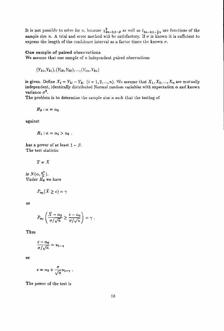
It is not possible to solve for n, because X~n-2;1-.13 as well as t2n-2;1-~-Y are functions of thesample size n. A trial and error method will be satisfactory. If a is known it is sufficient toexpress the length of the confidence interval as a factor times the known a.

One sample of paired observationsWe assume that one sample of n independent paired observations

is given. Define Xi = Y1i - Y2i (i = 1,2, ... ,n). We assume that X1,X2 , ••• ,Xn are mutuallyindependent, identically distributed Normal random variables with expectation a and knownvariance a 2 •

The problem is to determinc thc sample size n such that the testing of

Ho : a = ao

against

has a power of at least 1 - f3.The test statistic

T=X

is N(a, C7:).Under Ho we have

or

(X-ao c-ao)

Pao a/Vii ~ a/vn =I .

Thus

c- aoa/Vii = Ul--y

or

ac= ao+ ViiU1--y.

The power of the test is

18

= P(x ~ -0 +U1-"Y)

with

From the probability requirement

it follows that

Then

satisfies the requirement. From this it follows that

or

For given 7 and f3 and the difference 0:1 - 0:0 expressed as a multiple times (1, the neededsample size can be found. In most cases rounding-off upwards will be necessary to get aninteger value for the sample size n.For a left-hand sided alternative the quantity 6 is negative, but the same formula for n (withonly the absolute value of 0:1 - 0:0 of interest) can be used.For two-sided testing of

Ho : 0: = 0:0

against the two-sided alternative

19

HI: a =I ao

using the test statistic X, H 0 will be rejected if

The power of this test against an alternative a = al is equal to

= 1- P(lx + 61 < vI-b)

::: 1 - P(-u 1 - 0 < v < 1/ 1 - 6) .I-p' A 1-:j")'

The requirement that the power has to be at least 1 - f3 leads to

P(-ub - 6 < X < u1_ b - 8) = f3 .

If fJ is positive and sufficiently large, then P(x ~ -u1_ b - IS) can be neglected. Thus therequirement reduces to

P(x < u1-h - 6) = f3 .

From this it follows that

or

If 6 is negative and sufficiently large, then

f3 = P(-u1-h - 8 < X < -0 + lI1-h)

20

~ P(-U 1 - 0 < V) .l-i'Y A

Thus

or

Thus combining the two results:

which gives

Often a rounding-off to above is necessary to guarantee that the power is at least 1 - p.The case that u is unknown and has to be estimated by 52 (the pooled variance estimator;see section 3) can be dealed with in an analogous manner. The only difference is u to bechanged into tn-l'

A different approach is to put the requirement that

P(2tn - l;l-h In ~ L) 2: 1 - ;3 .

The left-hand side can be written as follows

P(2fn - lil-h In ~ L)

_P(2 < n(n - 1) (L) 2)- Xn-l - 4t2 ;; ,

where t = tn-lil-~'Y' The quantities t and X~-l depend on n, so it is not possible to solveexplicitely for n, but a trial and error method will work in practice to determine the requiredn. Often a rounding-off to above will be necessary.

21

5. The number of observations: Nonparametric situation

In this chapter we shall discuss the problem of determining the number of observations in somenonparametric situations. In other words for some familiar nonparametric or distribution-freetests we shall determine the minimal sample size such that the tests have power of at least1 - f3 against alternatives that differ sufficiently from the hypothesis being tested. In ourdiscussion we shall consider the Sign Test, the \Vilcoxon Signed Rank Test and the WilcoxonTwo-Sample Rank Test.Our starting point is a ,-level test \vith test statistic 1'. In the classical situation we had todetermine the sample size such that the requirement is met that the power against a param­eter value (which differs from the null hypothesis) is sufficiently large. In the nonparametricsituation there is in general not such a parameter. That is the reason we have to use adifferent approach. This approach is presented by Noether (1987).We suppose that l' is (approximately) distributed as N(J-L(1'), 0"2(1')). Under Ho we haveJ-L = J-Lo(1') and 0" = 0"0(1').For an upper-tailed test the critical region is defined by

l' > J-Lo(1') + u1-oyO"o(T) ,

and the power against the alternative lla is given by

= p ( > J-Lo(1') - 11(1') + -1)X - pO"o(T) U1--yP

with P = :.F{)) and P(X s; U1-oy) = 1 - ,.The requirement that the pmver of the test must be equal to 1 - f3 is met if

J-Lo(T) - J-L(T) -1pO"o(T) +U1-oyP = ul3( = -ul-l3)

or if

J-L(T) - J-Lo(T)0"0(1') = U1-oy + pUl-{3 •

With

Q(T) := {J-L(T) - J-Lo(T)}20"0(1')

the requirement is fulfilled if

22

We assume that p = 1. This is for instance true for shift alternatives. For alternatives thatare close to the null hypothesis this assumption is in general approximately correct. We get

and we can solve for the number of observations. For the one-sample problem discussed in

the previous chapter we have the test statistic T =Y = ~t Ii and QCfr) = (:iJ*f, andi=l

solving for n gives the same result we got in the previous chapter.

Sign TestAssume one sample of independent observations is given: YllY2 , ... , Yn • The associated con­tinuous random variable has median m. We want to test the null hypothesis

Ho : rn =rno,

with rno known. Subtractillg mo from the n obscrvaJions ]fo changes into

Ho : rn = o.

The Sign Test, which can be applied, has the followir,g test statistic

T = #{Y > O}.

Defining

p= P(Y > 0)

then

1/-leT) = np, /-lo(T) = - n

2

and

By the assumption of continuity we have Po(Y =0) =0, and Po(Y > 0) = !.To meet the power requirement we get

or

23

Against a known alternati\'c IIa : p(> ~) the required sample size can be determined. A

choice of p can be based on past experience. A different possibility is to put ~~~~~~ = c, then

G = c thus p = C~l'

For the Sign Test: p = yn(~p) = 2y'p(1- p) < 1 for p i= ~, so the determined sample size

is conservative.IT information on p, and thus on p, is available, then sometimes an improved estimate can begiven, using pU1-{3 instead of U1-{3 in the formula for n.

Wilcoxon Signed Rank TestGiven are n independent observations

from a continuous symmetric random variable. Suppose the distribution is symmetric aboutthe unknown location parameter 1n. 'Ve wish to test the null hypothesis

Ho : m = 0

versus the alternative hypothesis

HI: m > O.

It is possible to apply the \Yilcoxon Signed Rank Test. The test statistic T is defined asfollows. The absolute values of the n observations are ranked in increasing order of magnitude.The test statistic T is defined as the sum of the ranks associated with the positive observations.Under Ho the statistic T is asymptotically (for n -+ (0) Normally distributed with

n

ET = ~ L: i = ~n(n + 1)i=l

and

n

var T = ~ L: i 2 = 2\11(n +1)(2n + 1) .i=l

These expressions can easily be derived by noticing that under Ho the statistic T can ben

written as L: ZiR(fi) where R(1i) is the rank of 1i (after ranking the absolute values ofi=l

the n observations) and the Zi are independent and identically distributed random variableswith P(Zi = 1) = P(Zi = 0) = ~ so that E(Zd = ~ and var (Zi) = 1. Since T is a linearcombination of these variables, its exact mean and variance are easily determined under Ho.lt can be seen that

24

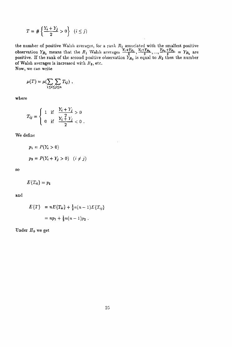
the number of positive Walsh averages, for a rank R I associated with the smallest positive

b . Y h 1 1 1 Y1+YR Y2 +YR YR +YRo servatlOll R 1 means t at t le R I 'Va S 1 averages ~,~, ... , 1 2 1 = YR1 arepositive. If the rank of the second positive observation YR2 is equal to R2 then the numberof Walsh averages is increased with R 2, etc.Now, we can write

peT) = JL(L :E Tij) ,l$i$.i$n

where

Tij = {

We define

1 if

o if

l'i+y., 3 > 0

l'i~y., 3 < 0

2 .

PI = P(Yi > 0)

P2 = P(Yi +l'j > 0) (i 1: j)

so

and

Under Ho we get

25

PI = ~

P2 = P(Yi +Yj > 0)

00 00

= f f fy( u)fy(r)dudv-00 -tl

00

= f {l- Fy(-v)}Jy(v)dv-00

00

= f Fy(v)fy(v)dv-00

From this it follows that

Q(T) = {np1 + ~n(n-l)]J2 -In(11~+ 1)}2[i4n(n +1)(2n +1)]2"

for sufficiently large n. The power requirement results in

or

_ 1( + )2( 1)-2n - 3 '111-')' '111-/3 ]J2 - 2 .

In practice we can make a choice of ])2 based on the ratio r = 'im-~':F7.;;+

get P2 = "~1 .

We see that the required sample size for the Sign Test is smaller than the size for the WilcoxonSigned Rank Test if and only if (approximately)

1( + )2( 1 )-2 1( )2(. 1)-2:4 '111-')' '111-/3 PI - 2 < 3 '111-')' + '111-/3 ]J2 - 2

or

26

or

For a number of distributions PI and P2 can be determined and the tests can be compared.

The two-sample test of WilcoxonThe test of Wilcoxon for two independent samples

drawn from continuous distributions to test the null hypothesis

against the alternative that Y2-obscrvations would tend to be larger than YI-observations.To detect this alternative we want to reject lIo when the sum ranks of Y21, Y22 , ••• , Y2n in thecombined sample are large in some sense. However, instead of measuring the tendency of thesum of Y -ranks to be large, we use the statistically equivalent test statistic of Mann-Whitney.The test statistic of Mann-Whitney U is defined as

m n

u =2:2:Dij ,i=1 j=1

where the indicator random variables are defined as

D .. = {1 if Y2j > }'iitJ 0 if Y2j < I'ii

for all i and j. In words: U is defmed as the llumLer of times a YI-observation precedes a Y2 ­

observation in the combined G~'dered arrangement of the two samples into a single sequenceof N = Tn +n variables increasing in magnitude.We get

00 tI=! ! !y2 (v)fYl(U)dudv-00 -00

00

= ! FY1(V)fY2(V)dv .-00

Then

27

m n

E{U} = LLE(Dij)i=l j=l

=mnp.

Under Ho : 'FY1(X) = Fyz(x) for all x' we get

00

p = ! FY1(V)fYl(V)dv-00

The null and alternative hypothesis can be formulated more precisely as p = l versus p > l.Thus

Eo{U} = lmn.

For the variance var U we get

var U = var{L L Dij}j

m

=L L var Dij +2:2: 2: cov (Dij, Dile )+i j i=ll:$jik:$n

n

+LL L cov(Dij,Dhj )+j=ll:$#h:$m

+L L L L co\' (Dij , Dhk) .l:$i;th:$m l:$j#:$n

The random variables Dij are Bernoulli variables with

var Dij = p - p2 = p( 1 - p)

COV(Dij, Dhk) = 0 for i i= 11, and j i= k

28

where

00

= J{1-FY2(X)}2fy1(x) dx-00

and

00

= JFfl(X)fY2(X)dx .-00

From this it follows

var U = mnp(l - p) +mn(n - l)(Pl _ p2)+

'When Fy2(x) = Fy1(x), thus under Ho, it can easily be proved that Pl = ~ = P2" Then

varoU = l12mn(N +1) "

With

m = f Nand n = (1 - J)N

we find

_ 12{f(1 - J)N 2p - ~f(l - f)N2p- f(l - f)N2(N +1)

~ 12Nf(1- J)(p-!? "

Thus the power requirement gives the next result

A t" t f - P(Y2>Yl) . t" t f - rn es Ima eo r - P(Y2<Yd gIves an es Ima eo p - rH"

29

6. Analysis of variance and nonparametric analysis of some specific designs

In this chapter the analysis of some designs will be indicated. In many experiments theassumption of Normality is quite commonly made for the data analysis. However, there areexperimental situations where this Normality assumption is not realistic. Nonparametricmethods are methods for which the validity does not depend on the underlying distributionof the observations.The purpose of this chapter is to give an overview of a number of classicaltests in some specific designs, side by side by a more or less comparable nonparametric analy­sis. For more detailed information we refer to Van del' Laan and Verdooren (1987). In generalwe shall suppose that the observations have been drawn from continuous distributions, henceties will occur with probability zero.

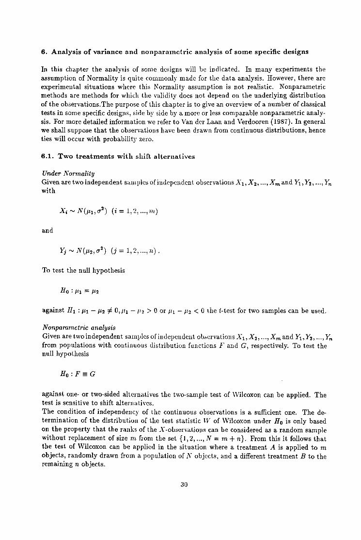
6.1. Two treatments with shift alternatives

Under NormalityGiven are two independent samples of independent observations XI, X 2 , ••• , X m and Yb Y2 , ... , Yn

with

and

To test the null hypothesis

Ho : III = 112

against III : III - 112 -# O,lll -112 > 0 or fli - fl2 < 0 the t-test for two samples can be used.

Nonparametric analysisGiven are two independent samplcs of independent obbcrvations XI, X 2 , ... , X m and Yb Y2 , ••• , Ynfrom populations with continuous distribution functions F and G, respectively. To test thenull hypothesis

Ho : F= G

against one- or two-sided alternatives the two-sample test of Wilcoxon can be applied. Thetest is sensitive to shift alternatives.The condition of independency of the continuous observations is a sufficient one. The de­termination of the distribution of the test statistic TV of Wilcoxon under Ho is only basedon the property that the ranks of the X -observations can be considered as a random samplewithout replacement of size m flOIll the set {1, 2, ... , N = m +n}. From this it follows thatthe test of Wilcoxon can be applied in the situation where a treatment A is applied to mobjects, randomly drawn from a population of N objects, and a different treatment B to theremaining n objects.

30

6.2. More than two treatments with shift alternatives

Under NormalityGiven are k(> 2) independent samples of independent observations Xi1, Xi2, ... , Xini (i =1,2, ,k) from a classification A with classes A ll A2: ... ,AIe • Assume Xii"" N(lti,a2), j =1,2, , ni. To test the null hypothesis

Ho : 1t1 = 1t2 = ... = Pie

against H l : 'at least one pair of p's is unequal' the analysis of variance F-test can be used.The test statistic is

MSA 1e-1F = MSE Ho FN _ 1e

Ie SS 1 SSEwith N ="'"' ni, M SA = --"-. ,AISE = -.-- and the Sum of Squares of A equals

~ k-l J\'-k1=1

and the Sum of Squares of Error equals

Ho is rejected for sufficiently large yalues.

Nonpammetric analysisGiven are k(> 2) independcllL samples of independent observation XillXi2 ... ,Xin, (i =1,2, ... , k) drawn from populations with continuous distribution functions Fi. To test

it is possible to apply the test of Kruskal-\Vallis with test statistic

K = 12{N(N +1)}-1 2:= ni(Ri. - .k..)2 ,i

where Rij is the rank of Xij in the combined sample of N observations. The test is sensitiveto shift alternatives.

6.3. More than two treatments with ordered alternatives

31

Under NormalityFor the case of k independent samples we are interested in the comparison of k(> 2) orderedlevels Zl,Z2, ... ,Zk of a quantitative treatment.4. \Ve assume JLi = <p(Zi), i = 1,2, ... ,k, andwish to test

Ho : <p(z) = f30 + f31z

against the alternative hypothesis H 1 : '<p(z) is more complex than linear'.We define the sum of squares for the linear trend of A, denoted by S S L, as

The test statistic is

SSA - SSL(k - 2)MSE '

which is under Ho distributed as F~-=-~. Sufficicutly large values lead to rejection of Ho.

Nonpammetric analysisIt is possible to consider in the k-sample situation an ordered alternative

with at least one strict inequality sign for at least one x. Two possible tests are suggested:the test of Jonckheere-Terpstra and Chacko-Shorack, respectively. In the case of regularshifts (horizontal distances between the distribution functions are more or less equal) the testof Jonckheere-Terpstra is recommended. In the case of (strong) irregular shifts the test ofChacko-Shorack is preferable. The test statistic T of Jonckheere-Terpstra is defined as

where Tij is the number of cases that an observation from sample i is smaller than an obser­vation from sample j (1::; i < j ::; k). For large values of ni is T under Ho approximatelyNormally distributed with

ET = ~(N2 - Lnni

and

32

The test statistic of Chacko-Shorack can be determined as follows. Under Ho one expectsroughly fl. :::; 1'2. :::; ... :::; Tk. (the lower case character l' is the outcome of the same capitalcharacter R; see Section 6.2). If this is not so for a pair, then the members of such a pairare put together (with sample size ui) and again the average rank is computed. We continuewith this operation, until

where ft. (i = 1,2, ... ,1) arc the average ranks of the ultimate groups with nt observations.The test statistic is

R"* - 12 ~ * {l""* 1(1\T )}2- N(N + 1)~ nj Lj. - 2 . +1 .

For large values of nl = n2 = ... = 11k we have approximately

1c

P(I<* ~ c) = L:Pi,kP(;\L1 ~ c) ,i=2

where some Pi.le can be found in the next table.

k

2 3 4 5 62 1.. !.!. ~ ~

~ 24 V 3603 1 5

6 f 214 194 24 1

12 114

;)120 4

18

6 7?ri

6.4. Two treatments in randomized blocks of size two (orthogonal design)

Under NormalityIn a block Bj of size 2 (j = 1,2, ... , b) two treatments .41 and A 2 are assigned at random tothe units of the block. We assume

l'ij = ai + f3j +Eij (i = 1, 2;j = 1,2, ... , b) ,

where ai is the expected effect of Ai, f3j is the expected effect of Bj and Ei/S are independentN(O, (72) random variables.To test

against HI : al ::j:. a2 the test statistic M~~ can be used, where MSA = ~:1 with SSA =

b-1t (2;:l'i j)2 - (2bt 1 (~)ij) 2 and MSE = ~::f with1=1 3 t,)

33

SSE = ~1i~ - i~ (~Yij) 2 - SSA .• ,3 3'

Under Ho :~~ is distributed as FLI' Large values lead to rejection of Ho.

Nonparametric analysisAssume b independent pairs of observations (XI, 1'1), (X2,1'2), ... , (XI., 1'1.) are given. A pairis for instance the result of two treatments applied in a block. To test

R o ; P(Xi > Yi) = P(Xi < Yi) =! for all i

against HI ; Ho is not true, the Sign test can be used. In general a more powerful test is theWilcoxon Signed Rank test. With this test the null hypothesis Ho: 'Zi = Xi-Yi(i = 1,2, ... ,b)is symmetrically distributed around zero.' can be tested.

6.5. More than two treatInents in randomized blocks (orthogonal design)

Under Normalityt

Given are b blocks Bj(j = 1,2, .."b) of size I>nij. In each block t(> 2) treatmentsi=1

AI, A2 , ••• , At are applied at random, treatl1lent Ai in block B j is allotted at random tomii units. We consider an orthogonal design, thus the relation mij = mi.m.j/m.. holds. Themodel is

}ijk = Ui + /3i +Eijk (i = 1,2, ... , t; j = 1,2, .. " b; k = 1,2, ... , mij)

with Ui the expected effect of Ai, /3j that of Bj and Eijk are i.i.d. N(O, (12) r.v.To test H 0 : u1 = u2 = ... = 0t the test statistic is

T = MSAMSE

with

MSA = SSAt - 1

S S A = 2: (2: Yiik) 2 / mi, _ ~ (2: 1'ij k) 2"le m., "le• 3, ',3.

MSE = (m.. - t - b+1)-1SEE

SSE = 2: li~k - 2: (2: l'ijk) 2 /m.j - SSA .i,j,le i i,k

34

Under H o the statistic T is distributed as F~~.:-t-b+1' Large values ofT lead to rejection of Ho.

Nonparametric analysisTo test the null hypothesis of no treatment effect, the observations Yijk within block Bj areranked in increasing order of magnitude with ranks 1,2, ... , m.j (j = 1,2, ... , b). These ranksare Rijk. The test statistic is defined as

Q. ~ 12N {~m';(m;+ I)} -,~mi.' {Ri" -!~ ",,;(m.; + I)rwith Ri.. the sum of the ranks for treatment Ai. Qo has under Ho asymptotically a X~-l­

distribution. The condition of the approximation and the treatment of ties can be found inBenard and Van Elteren (1953).If mij =1 for all i and j, the test statistic Q0 simplifies to the test statistic of Friedman.An alternative procedure based on standardized ranks has been proposed by De Kroon andVan der Laan (1983). They suggested as test statistic

with

and

Under Ho the statistic Q has asymptotically (for m.j -+ oc) a XLl-distribution.

6.6. More than two treatments in randomized blocks and ordered alternatives(orthogonal design)

Under NormalityAs described in Section 6.3 we are interested in the investigation of a quantitative treatmentA with levels Zt, Z2, ... , Zt. 'Ve consider a randomized block design with one observation percell and the model

Xij = J.t +Qi + {3; +Bii' (i = 1, 2, ... , t; j = 1, 2, ... , b) ,

where J.t is the general mean, O'i is the deviation from J.t for treatment Ai, Pi that of blockBj(I: Qi = 0 =I: (3;) and Eij are LLd. .N(O, 0 2 ) r.v..

i ;

To test Ho: '4>(z) = 'Yo; + 'YlZ in block j' against lI1 : '4>(z) is more complex than linear', westart with the computations as described in Section 6.5 for m = l.The test statistic is

35

SSA - SSL(t - 2)MSE

with

SSL = {~bzl- :t(~bZi)2}-l{~ZiXij - :t(~bZi)(~Xij)}2I I t,' t t,'

and has under Ho a Ftt~2l)(b_lrdistribution. Large values lead to rejection of Ho.

Nonparametric analysisIn Friedman's block design with one observation per cell, we assume

CEai = 0 = "£j3j) with Eij independently and continuously distributed random variableswhich are identically distributed in each block. For testing Ho of no treatment effect againstH l : al ::; a2 ::s ... ::s at with at least one strict inequality sign, the test statistic of Page(1963)

can be used. Ranking within blocks, the same as for Friedman's test. Ho is rejected when Lissufficiently large. For large values of b the statistic L has approximately a Normal distributionwith

EL = ~bt(t + 1)2

and

L 1 b(t3 _ t 2var = 144(t - 1) ) .

6.7. More than one treatment in a Balanced Incomplete Block Design (BIBD)

Under NormalityIt is in practice possible that a block can only contain at most k experimental units. Apossible reason may be that blocks with a size larger than k are not homogeneous enough. Ift > k we need a so-called incomplete block design. Suppose that for t treatments in blocksof size k a design can be constructed for which

- every treatment occurs on r units- every pair of treatments occurs in Aof the b blocks.

36

If b blocks are required, then rt = bk and A( t - 1) = r(k - 1). Such a design (if it exists) iscalled a Balanced Incomplete Block Design. Randomization of blocks, treatments and unitsis necessary.To test II0 : a1 = a2 = ... = at we use the test statistic

MSAT= MSE'

Let Ti be the total of the Yij'S of treatment Ai, Bi be the total of the blocks in which treatmentAi occurs. Then we define

and

MSA = SSAt-1

SSA = A~k ~(kQi)2I

MSE = (tr - t - b+ l)-lSS£

SSE =~li~ - ~ 2;::(Block j)2 - SSA ,1.3 3

where Block j is the total uf the k observations in block j. T has under Ro a Fi,:-:':t-b+I­distribution.Large values of T lead to rejection of Ro.

Nonparametric analysisIn a BIBD the rank test of Durbiu can be applied, which is based on the test statistic

12(t - 1)D = '"{R· - !r(k + 1)}2

rt(k 2 - 1) 7 · 2

with Ri the sum of the ranks for Ai after ranking within blocks where Ai occurs.The asymptotic distribution of D under JIo is X~-l' The exact distribution can be found inVan del' Laan and Prakken (1972).

6.8. Interaction in a two-way la~'out

Under NormalityAssume we have two factors A and B, with A on s levels and B on t levels. A completefactorial experiment of A and B is performed, where each treatment combination has beenexecuted m(> 1) times. The design is a completely randomized design with stm units.Let Xijlt be the k-th observation of the treatment combination (Ai,Bj) with the model

37

(i = 1,2, ... ,s;j = 1,2, ... ,t; k = 1,2, ... ,m),

where J.l is the general mean, ai is the deviation from the general mean for Ai,f3j that for Bjand "Iij is the deviation from the general mean due to the non-additivity effect or interactioneffect of Ai and Bj. Then the following holds:L:ai = 0 = L:f3j and 2:::»'ij = 0 = I:>rii (for all j and i, respectively). The error terms

i j i j

Eij1c are LLd. N(O,0'2) random variables.To test

Ho : "Iij = 0 for all

the test statistic is

T= MSABMSE

with

and j

SSAB

MSE

SSE

1 SSEst(m - 1)

'" 2 1 ""' ,""' ~ 2= L.", X ij1c - - L.",(L.", Xijk) •i,i,1c m i,i Ie

T has under Ho a F;:{~2~)1)-distribution with a righthand-sided critical region.

Nonparametric analysis(Testing against rank-interaction)The concept of rank-interaction, a nonparametric concept of interaction, has been introducedby De Kroon and Van del' Laan (1981). In each cell (i,j), a combination of the i-th level offactor A and the j-th level of factor B, are given m(> 1) observations. The error terms Eij1c

are independently and identically distributed random variables with continuous distributionfunctions and E(Eij1c ) = O(i = 1,2, ... ,sij = 1,2, ... ,t and k = 1,2, ... ,m). We wish to

Ho : f31 + 'Yil = f32 + 'Yi2 = ... = f3t + 'Yit for i = 1,2, ... ,s.

38

The choice of a test procedure depends on the alternative hypothesis one is interested in.Depending on which alternatiYe is thought to be important in the practical problem, one canchoose one of three statistics 1',1'1 and 1'2. As an omnibus test we have

•1'= LKi,

t::::1

where ](i is the Kruskal-Wallis statistic computed for the classification B within class i offactor A. The test statistc 1'1 is defined to be the Friedman test statistic for the case of sblocks of ranking over t classes of factor B, each class containing m observations. 1'1 willbe used if differences between the /3/s are interesting. The test statistic T2 = T - T1 canbe used if one is mainly concerned \vith rank-interaction. Roughly speaking rank-interactioncan be understood as the phenomenon where the ranks of the response variable X for thelevels of factor B are different for some levels of factor A. In other words not all deviationsfrom zero of the 'Yii'S are of interest, but only those deviations that give discordance betweenthe rankings within the levels of factor A. If the rankings of

{31 + 'Yil,{32 + 'Yi2, ... ,{3t + ~fit (i = 1,2, ... , s)

are not identical for different values of i, we say that rank-interaction B*(A) exists. If theserankings are identical ("concordance"), rank-interaction B*(A) is said not to exist.It is also possible to use the statistics 1'1 and 1'2 simultaneously, each at significance levela/2, rejecting Ho if at least one of the outcomes of 1"1 or 1'2 is larger than or equal to thecorresponding critical value. In this way it is possible to carry out an omnibus test with thepossibility of detecting simulLaneously which component of Ho is not true, This procedure issomewhat, probably slightly, conservative. For critical values for all three tests and furtherdetails of the various procedures we Iefer to De Kroon and Van del' Laan (1981). Extensivetables with critical vlaues can be found in Yan der Laan (1987). For power comparisons seeDe Kroon and Van del' Laall (1984.).

39

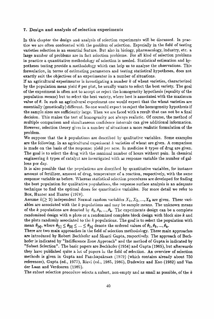
7. Design and analysis of selection experiments

In this chapter the design and analysis of selection experiments will be discussed. In prac­tice we are often confronted with the problem of selection. Especially in the field of testingvarieties selection is an essential feature. But also in biology, pharmacology, industry, etc. alarge number of problems are in fact selection problems. For all kind of selection problemsin practice a quantitative methodology of selection is needed. Statistical estimation and hy­potheses testing provide a methodology which can help us to analyse the observations. Thisformulation, in terms of estimating parameters and testing statistical hypotheses, does notexactly suit the objectives of an experimenter in a number of situations.If an agricultural experimenter is investigating a number k of wheat varieties, characterizedby the population mean yield 0 per plot, he usually wants to select the best variety. The goalof the experiment is often not to accept or reject the homogeneity hypothesis (equality of thepopulation means) but to select the best variety, where best is associated with the maximumvalue of O. In such an agricultural experiment one would expect that the wheat varieties areessentially (genetically) different. So one would expect to reject the homogeneity hypothesis ifthe sample sizes are sufficiently large. Then we are faced with a result that can not be a finaldecision. This makes the test of homogeneity not always realistic. Of course, the method ofmultiple comparison and simultaneous confidence intervals can give additional information.However, selection theory gives in a number of situations a more realistic formulation of theproblem.We suppose that the k populations aTe described by qualitative variables. Some examplesare the following. In an agricultural experimcnt k varieties of wheat are given. A comparisonis made on the basis of the response: yield pcr acre. In medicine k types of drug are given.The goal is to select the drug with the maximal number of hours without pain. In chemicalengineering k types of catalyst are investigated with as response variable the number of gal­lons per day.It is also possible that the populations are described by quantitative variables, for instanceamount of fertilizer, amount of drug, temperature of a reaction, respectively, with the sameresponse \'ariable as before. \Vhereas statistical selection procedures are developed for findingthe best population for qualitative populations, the response surface analysis is an adequatetechnique to find the optimal doses for quantitative variables. For more detail we refer toBox, Hunter and Hunter (1978).Assume k('?:. 2) independent NOl'lHal random variables Xl, X 2 , ... , Xle are given. These vari­ables are associated with the k populations and may be sample means. The unknown meansof the k populations are denoted by fh, 02, ... , Ok. The experiments design can be a completerandomized design with n plots or a randomized complete block design with block size k andthe plots randomly associated to the k populations. The goal is to select the population withmean 8[k]' where 8[1] ~ 8[2] ~ ... ~ O[Ie] denote the ordered values of 81,82, ... , 8le .There are two main approaches in the field of selection methodology. These main approachesare introduced by Robert Bechhofer and Shanti Gupta, respectively. The approach of Bech­hofer is indicated by "Indifference Zone Approach" and the method of Gupta is indicated by"Subset Selection". The basic papers are Bechhofer (1954) and Gupta (1965), but afterwardsthey have published quite a lot of papers in the field of selection. An overview of selectionmethods is given in Gupta and Panchapakesan (1979) (which contains already about 750references), Gupta (ed., 1977), Rizvi (ed., 1985, 1986), Dudewicz and Koo (1982) and Vander Laan and Verdooren (1989).The subset selection procedure selects a subset, non-empty and as small as possible, of the k

40

populations considered in order to include the best population with the probability require­ment that the probability of a Correct Selection is at least P*. A Correct Selection (CS)means in this context that the best population is an element of the selected subset. Thesubset selection approach has certain advantages in practice. It can be applied to analyse thedata after the experiment has been realized. In the context of this report we are interestedin designing an experiment. That is the reason we shall concentrate on the approach ofBechhofer: The Indifference Zone approach.

The Indifference Zone approach is an important approach for designing an experiment. Thegoal is to indicate the best population. It provides a value for the common sample size neededto meet certain probability requirements. A Correct Selection (CS) means in this contextthat the best population is indicated. The probability requirement is that the probability ofa CS is at least P*, whenever the best population is at least 6* away from the second best.The minimal probability P* can only be guaranteed if the common sample size n is largeenough. In the next section this procedure will be described in more detail.

Bechhofer's approach to selection: Indifference Zone proceduresAssume 1.~(?:. 2) independent populations denoted by G = (71"1,71"2, ... , 71"k) are given. The re­lated independent random variables are denoted by Yl , 1'2, ... ,Yk' The random variable 1i hascumulative distribution function F(y; Bi ) with the unknown real-valued parameter Oi E 0( i =1,2, ... ,k). Let 0 denote the parameter space {B: 0 = (B l ,02, ... ,Ok);Bi E 0,i =1,2, ... ,k}.The ranked parameter values are indicated by 0[1] :::; B[2] :::; .. , :::; B[k]' The population asso­ciated with B[i] will be denoted by 7i(i)' Usually in ranking the population 71"j is better than71"i if OJ > Oi. Then we define the population 71"(lc) associated with O[k] as the best population.The t(l :::; t < k) best populations are the populations 71"(lc-t+l)' 71"(k-t+2)' ••• , 71"(k)' If there aremore than t contenders because of tics, it is assumed that t of these are appropriately tagged.The goal of selection considered in this paper is to select an unordered set of t populationsassociated with the set {O[k-t+ll' B[Ie-t+ 2], ••• , O[Ie]}' In this context a correct selection meansthat the t best populations are selected.Let Oji denote a measure of distance between the populations x(i) and 71"(j) with 1 :::; i < j :::; k.

In case 0 is a location parameter, 6ji is usually defined as B[j] - B[i]'

The probability requirement that the probability of selecting the t best populations is at leastP* can be written as follm';s. Denoting the probability of a correct selection (CS) using aselection procedure R by P(C SIR) or P(C S), one can write the probability requirement asP(CS) ?:. P* for 0 E 0(6*) = {O ; tk-t+l,lc-t ?:. 6*}.

The experimenter has to specify positive constants ,. and P', where P' E ( ( ~ ) -, ,1) .

Usually the selection rule is based on sufficient statistics for B1 , B2 ••• , Ok, These sufficientstatistics are based on samples of common size n from the k populations.The general problem in this context is to determine the smallest common sample size n forwhich

inf P(CS) > P* .0(6·) -

This condition is called the P*-condition for the probability requirement. The infimum oftheP(CS) is evaluated over the subset 0(6*) of the parameter space O. 0(6*) is the so-calledpreference zone and OC(0*) is called the indifference zone.

41

Let us consider the situation of k Konnal populations with common known variance (12 inmore details. The selection rule R is based on the sufficient statistic Yi for Oi, where Yiis the mean of a sample of ni independent observation from 1ii(i = 1,2, ... ,k). The goal isto partition the set G into 2 subsets G1 and G2 with G = G1 U G2 , G1 n G2 = 0, G1 ={1l"(Ic- t+l), 1l"(Ic-t+2)' ... , 1l"(Ic)} and G2 = {TI(l)' 11"(2)' .•. , TI(k-t)}.The selection rule R is defined as follows. \Ve determine a subset S c G of size t on the basisof the sample means. Include in S the populations associated with

where X[l] ~ X[2] ~ ... ~ X[k] are the ranked sample means. The P*-condition is

peGS) = P[S = G110 E nco"')] = P[S = G1IOk-t+l,k-t ~ 0*] ~ P* .

We have for ni = nand }T(i) is the sample mean associated with 1l"(i):

00

~ t ! <p1c-t(z +T){l - <fI(z)}t-ld!J>(z) ,-00

where <p is the standard Konua1 distribution function and

! * -17=n20(1 .

The minimum of the P(GS) for R is at tained for the so-called Least Favourable Configuration(LFC) in n(0*), given by

0[1] = ... = O[Ic-t] = O[k-t-t-l] - f" = ... = B[k] - 0" .

The minimum sample size rCI!uired is the smallest integer n for which the P*-condition isfulfilled.For the LFC we have

00

PLFC(GS) = t ! <pk-t(z +T){l - <p(z)}t-1d<p(z) ,-00

which is an increasing function of 7 and tends to 1 as 7 tends to infinity. Hence, there is aunique smallest value 7 meeting the probability requirement. This value is the solution ofthe equation.

42

For the special case t = 1, the rule R selects the population associated with Y[k]' Then forthe P"-condition we have

00

~ / epk-l(Z +7)d<I>(z) ~ P* .-00

In order to meet the probability requirement in the case t =1 we have to choose:

_ (7(1)2n- .0"

In order to be sure that the common sample size is large enough to satisfy the probabilityrequirement, the computed value of 12 is rounded upward if it is not an integer. The quantityT, which depends on k and P*, can be computed by numerical integration. Some values canbe found in next table.

p~

k .90 .952 1.812 2.3263 2.230 2.7104 2.452 2.9165 2.600 3.0556 2.710 3.1597 2.797 3.242S 2.868 3.3109 2.930 3.3G8

10 2.983 3.4182·~ 3.391 3.810

Extensive tables for 7 can be found in for instance Gibbons, Olkin and Sobel (1977), TableA1, for various values of p. and k.An important function characterizing the "power" of a selection procedure is the OperatingCharacteristic curve (OC curve), defLlled as the P(CS) for the Generalized LFC: 0[1] =9[1e-l] =O[k] - 0, so P(C S) is a function of 6 (besides elk] and n).The following confidence statement can be made after the experiment has been conducted:

where 9. is the unknown population mean associated with the selected population. This1

statement can be made provided only 0*n2(1-1 = 7.

Normal populations with unknown (12Given are k Normal populations with unknown means and U1l1,110Wn equal variances, where

43

the common variance (72 is considered as a nuisance parameter. The goal is to select thebest population (associated with elk])' 'Vithout information about (72, it can be seen by in­creasing (72 that there is no common fixed sample size large enough such that the probabilityrequirement will hold for all possible values of (72. For if the true value of (72 is sufficientlylarge, the P(CS) will be arbitrarily close to k-1 , which is smaller than any reasonable valueof P*(k-1 < P* < 1).It is possible to use a good estimate of 0 2 by pooling the sample variances and use thisestimate as an approximation to 0 2 . Dechhofer, Dunnett and Sobel (1954) and Dunnett andSobel (1954) use a two-stage procedure. The first stage is used to estimate (72. The twostages together are used to reach a final decision. In Gibbons, Olkin and Sobel (1977) tablescan be found that make the execution possible.The case of unequal unknown variances is investigated by Dudewicz and Dalal (1975). Bech­hofer (1960) and Bechhofer, Santner and Turnbull (1977) discuss two-factor experiments.Complete factorial experiments are considered in Dudewicz and Taneja (1980), Lun (1977)and Bechhofer (1977). Selection problems in balanced complete and incomplete block designsare considered by Rasch (1978).

44

8. Final remarks

In 'Design and Analysis of experiments' by Doornbos (1990) one can find a number of generaldesigns and the correspondillg analyses.The possibility of combining nunparametric tests for the analysis of factorial designs is dis­cussed in Van der Laan and Weima (1983).

45

Literature

AFSARINEJAD, K. (1983). Balanced repeated measurements designs. Biometrika 70, 199­204.

AGRESTI, A. (1984). Analysis of Ordinal Categorical Data. John Wiley & Sons, Inc., NewYork.

ALTHAM, P .M.E. (1971). The analysis of matched proportions. Biometrika 58, 561-576.

ANSCOMBE, F.J. and TUKEY, J.W. (1963). The examination and analysis of residuals.Technometrics 5, 141-160.

BECHHOFER, R.E. (1954). A single-sample multiple decision procedure for ranking meansof normal populations with known variances. Ann. Math. Statist. 25, 16-39.

BECHHOFER, R.E. (1960). A multiplicative model for several factors. J. Amer. Statist.Assoc. 55, 245-264.

BECHHOFER, R.E. (1977). Selection in factorial experiments. Proc. of the 1977 WinterSimulation Conference (Eds. H.J. Highland, R.G. Sargent and J.W. Schmidt) held atthe National Bureau of Standards, Gaithersburg, Maryland, 65-70.

BECHHOFER, R.E., DUNNETT, C.W. and SOBEL, M. (1954). A two-sample multiple deci­sion procedure for ranking means of normal populations with common unknown vari­ance. Biometrika 41, 170-176.

BECHHOFER, R.E., SANTNER, T.J. and TURNBULL, B.W. (1977). Selecting the largest in­teraction in a two-factor experiment. Statist. Decision Theor. and Related Topics - II(Eds. S.S. Gupta and D.S. Moore), Acad. Press, New York, 1-18.

BENARD, A. and ELTEREN, PH. VAN (1953). A generalization ofthe method of m rankings.Kon. Nederl. Akad. van Wetensch., Proceed. Series A 56,358-369.

BERENBLUT, 1.1. and WEBB, G.1. (1974). Experimental design in the presence of autocor­related errors. Biometrika 61, 427-437.

BISHOP, S.H. and JONES, B. (1984). A review of higher-order cross-over designs. Journalof Applied Statistics 11, 29-50.

Box, G.E.P. (1957). Evolutionary Operation: A Method for Increasing Industrial Produc­tivity. Applied Statistics 6,81-101.

Box, G.E.P. and DRAPER, M.R. (1969). Evolutionary Operation. John Wiley & Sons,Inc., New York, London.

Box, G.E.P. and DRAPER, N.R. (1987). Empirical Model Buidling and Response Surfaces.John Wiley & Sons, Inc., New York, London.

Box, G.E.P., HUNTER, W.G. and HUNTER, J.S. (1978). Statistics for Experimenters. JohnWiley & Sons, New York.

46

BROEMELING, L.D. (1985). Bayesian Analysis of Linear Models. Marcell Dekker, NewYork.

CHENG, C.S. and WU, C.F. (1980). Balanced repeated measurements designs. Annals ofStatistics 8, 1272-1283. Corrigendum (1983) 11, 349.

COCHRAN, W.G. and Cox, G.M. (1957). Experimental designs. 2nd ed., John Wiley &Sons, Inc., New York-London.

CONOVER, W.J. and IMAN, R.L. (1981). Rank transformations as a bridge between para­metric and non-parametric statistics. The American Statistician 35, 124-129.

CORSTEN, L.C.A. (1984). Ontwerp en analyse van experimenten (in Dutch). VakgroepWiskunde, Landbouwhogeschool Wageningen.

Cox, D.R. (1966). Planning of Experiments. John Wiley & Sons, Inc., New York-London­Sydney.

Cox, D.R. (1984). Interaction. International Statistical Review 52, 1-31.

DAS, M.N. and GIZI, N.C. (1979). Design and Analysis of Experiments. Wiley EasternLimited, New Delhi, Bangalore, Bombay, Calcutta.

DAVIES, O.L. (ed.) (1963). Design and analysis of industrial experiments. 2nd. ed., Oliverand Boyd, Edinburgh, London.

DAVIS, A.W. and HALL, W.B. (1969). Cyclic change-over designs. Biometrika 56, 283­293.

DOORNBOS, R. (1990). Design and analysis of experiments. Report Department of Mathe­matics and Computing Science, Eindhoven University of Technology.

DUDEWICZ, E.J. and DALAL, S.R. (1975). Allocation of observations in ranking and selec­tion with unequal variances. Sankhya B 37, 28-78.

DUDEWICZ, E.J. and Koo, J.O. (1982). The complete categorized quide to statistical se­lection and ranking procedures. Series in Math. and Management Sciences, Vol. 6,Amer. Sciences Press, Inc., Columbus, Ohio.

DUDEWICZ, E.J. and TANEJA, V.S. (1980). Ranking and Selection in designed experiments:complete factorial experiments. Techn. Report 210, Ohio State Univ.

DUNNETT, C.W. and SOBEL, M. (1954). A bivariate generalization of Student's t distribu­tion, with tables for certain special cases. Biometrika 41, 153-169.

EVERETT, B.S. (1977). The Analysis of Contingency Tables. Chapman and Hall, London.

FEDERER, W.T. (1955). Experimental Design, Theory and Application. MacMillan and Co.

FEDEROV, V.V. (1972). Theory of optimal experiments, Academic Press, New York andLondon.

FINNEY, D.J. (1960). An introduction to: The theory of experimental design. The Universityof Chicago Press, Chicago.

47

FISHER, R.A. (1966). The Design of Experiments. 8th ed., Hafner Publishing Company,New York.

FLEISS, J.L. (1986). The Design and Analysis of Clinical Experiments. John Wiley & Sons,Inc., New York.

FLETCHER, D.J. (1987). A new class of change-over designs for factorial experiments.Biometrika 74, 649-654.

FLETCHER, D.J. and JOHN, J .A. (1985). Changeover designs and factorial structure. Jour­nal of the Royal Statistical Society B 47, 117-124.

GENTLEMAN, J.F. and WILK, M.B. (1975). Detecting outliers in a two-way table: 1. Sta­tistical behavior of residuals. Technometrics 17, 1-14.

GIBBONS, J.D. (1985). Nonparametric Statistical Inference. Marcell Dekker, New York.

GIBBONS, J.D. OLKIN, 1. and SOBEL, M. (1977). Selecting and Ordering populations: Anew statistical methodology. John Wiley & Sons, Inc., New York.

GUPTA, S.S. (1965). On some multiple decision (selection and ranking) rules. Technometrics7,225-245.

GUPTA, S.S. (Ed.) (1977). Ranking and selection. Special Issue, Comm. Statist., Theor.Meth. A6.

GUPTA, S.S. and PANCHAPKESAN, S. (1979). Multiple decision procedures: Theory andmethodology of selecting and ranking populations. John Wiley & Sons, New York­London.

HAALAND, P.D. (1989). Experimental Design in Biotechnology. Marcell Dekker, New York.

HEDAYAT, A. and AFSARINEJAD, K. (1975). Repeated measures designs, 1. in A Survey ofStatistical Design and Linear Models (ed. J.N. Srivastava). North-Holland, Amsterdam.

HEDAYAT, A. and AFSARINEJAD, K. (1978). Repeated measures designs, II. Annals of Statis­tics 6, 619-628.

HERZBERG, A.M. and Cox, D.R. (1969). Recent work on the design of experiments: Abibliography and a review. J. R. Statist. Soc. A 132, 29-67.

HICKS, C.R. (1964). Fundamental concepts in the design of experiments. Holt, Rinehartand Winston, New York and London.

HOLLANDER, M. and WOLFE, D.A. (1973). Nonparametric Statistical Methods. John Wi­ley & Sons, Inc., New York.

JOHN, J .A. (1987). Cyclic Designs. Chapman and Hall, London and New York.

JOHN, P .W.M. (1971). Statistical Design and Analysis of Experiments. The MacMillanCompany, New York, London.

JONES, B. and KENWARD, M.G. (1990). Design and Analysis of Cross-Over Trials. Chap­man and Hall, London-New York.

48

KEMPTHORNE, O. (1952). The Design and Analysis of Experiments. John Wiley & Sons,Inc., New York-London.

KHURI, A.I. and CORNELL, l.A. (1987). Response Surfaces: Design and Analyses. MarcellDekker, New York.

KISH, L. (1987). Statistical Design for Research. John Wiley & Sons, Inc., New York.

KOCH, G.G. (1972). The use of non-parametric methods in the statistical analysis of thetwo-period change-over design. Biometrics 28, 577-584.

KOCH, G.G., AMARA, LA., STOKES, M.E. and GILLINGS, n.B. (1980). Some views onparametric and non-parametric analysis for repeated measurements and selected bibli­ography. International Statistical Review 48, 249-265.

KROON, J.P.M. DE and LAAN, P. VAN DER (1981). Distribution-free test procedures intwo-way layouts; a concept of rank-interaction. Statistica Neerlandica 35, 189-213.

KROON, J.P .M. DE and LAAN, P. VAN DER (1983). A generalization of Friedman's rankstatistic. Statistica Neerlandica 37, 1-14.

KROON, J.P.M. DE and LAAN, P. VAN DER (1984). A comparison of the powers of a gen­eralized Friedman's rank test and an aligned rank procedure based on simulation. Sta­tistica Neerlandica 38, 189-198.

LAAN, P. VAN DER (1987). Extensive tables with critical values of a distribution-free testfor rank-interaction in a two-way layout. Biuletyn Oceny Odmian 12, 195-202.

LAAN, P. VAN DER and PRAKKEN, J. (1972). Exact distribution of Durban's distribution­free test statistic for Balanced Incomplete Block Designs, and comparison with thechi-square and F-approximation. Statistica Neerlandica 26, 155-164.

LAAN, P. VAN DER and VERDOOREN, L.V. (1987). Classical analysis of variance methodsand nonparametric counterparts. Biometrical Journal 29, 635-665.

LAAN, P. VAN DER and VERDOOREN, L.V. (1989). Selection of populations: An overviewand some recent results. Biometrical Journal 31, 383-420.

LAAN, P. VAN DER and WEIMA, J. (1983). Application of the combination of some non­parametric tests for simple factorial designs (in Dutch). Kwantitatieve Methoden 10,121-138.

LOUIS, T .A. (1988). General methods for analysing repeated measures. Statistics in Medicine7,29-45.

LUN, F.W. (1977). Selection in factorial experiments. Project Report, Statistics 828, OhioState Dniv.

MATTHEWS, J.N.S. (1988). Recent developments in crossover designs. International Statis­tical Review 56, 117-127.

MEAD, R. (1988). The design of experiments: Statistical principles for practical applications.Cambridge University Press, Cambridge, New York.

49

MENDENHALL, W. (1968). Introduction to Linear Models and the Design and Analysis ofExperiments. Wadsworth Publishing Company, Inc., Belmont, California.

MONTGOMERY, D.C. (1984). Design and Analysis of Experiments. 2nd ed., John Wiley &Sons, Inc., New York.

MYERS, R.H. (1971). Response Surface Methodology. Allyn and Bacon, Inc., Boston.

MYERS, R. (1976). Response Surface Methodology. Edwards.

NOETHER, G.E. (1987). Sample size determination for some common nonparametric tests.J. Amer. Statist. Assoc. 82,645-647.

OTTESTAD, P. (1970). Statistical Models and their Experimental Application. Griffin's Sta­tistical Monographs and Courses, London.

PATEL, H.I. (1986). Analysis ofrepeated measures designs with changing covariates in clin­ical trials. Biometrika 73, 707-715.

PATTERSON, H.D. (1973). Quenouille's change-over designs. Biometrika 60, 33-45.

PIGEON, J.G. and RAGHAVARAO, D. (1987). Crossover designs for comparing treatmentswith a control. Biometrika 74, 321-328.

PLACKETT, R.L. (1981). The Analysis of Categorical Data. Griffin, London.

POCOCK, S.J. (1983). Clinical Trials. John Wiley & Sons, Inc., New York.

QUENOUILLE, M.H. (1953). The Design and Analysis of Experiment. Griffin's StatisticalMonographs & Courses, London.

RAGHAVARAO, D. (1971). Construction and Combinatorial Problems in Design of Experi­ments. John Wiley & Sons, Inc., New York.

RAGHAVA RAO, D. (1989). Crossover designs in industry, in Design and Analysis of Experi­ments, With Applications to Engineering and Physical Sciences (ed. S. Gosh), MarcellDekker, New York.

RAKTOE, B.L., HEDAYAT, A. and FEDERER, W.T. (1981). Factorial Designs. John Wiley& Sons, Inc., New York.

RAsCH, D. (1978). Selection problems in Balanced Block Designs. Biometrical Journal 20,275-278.

RIZVI, M.H. (Ed.) (1985, 1986). Modern Statistical Selection. Part I and II. Proceedingsof the Conference "Statistical ranking and selection - Three decades of development".Univ. of California at Santa Barbara, Dec. 1984, Amer. J. of Math. and ManagementSciences, Vol. 5 (Nos. 3 & 4) and Vol. 6 (Nos. 1 & 2).

SANTNER, T.J. and TAMHANE, A.C. (1984). Design of Experiments (Ranking and Selec­tion). Marcell Dekker, New York-Basel.

SCHEFFE, H. (1959). The Analysis of Variance. John Wiley & Sons, Inc., London-NewYork.

50

SEARLE, S.R. (1971). Linear Models. John Wiley & Sons, Inc., New York, London.

SEN, M. and MUKERJEE, R. (1987). Optimal repreated measurements designs under inter­action. Journal of Statistical Planning and Inference 17, 18-91.

STEFANSKY, W. (1972). Rejecting outliers in factorial designs. Technometrics 14, 469-479.

TUKEY, J.W. (1951). Quick and dirty methods in Statistics, Part II, Simple analysis forstandard designs. Proceedings of the fifth annual Convention. American Society forQuality Control, 189-197.

\\TARE, J.H. (1985). Linear models for the analysis of longitudinal studies. The AmericanStatistician 39, 95-101.

51

List of COSOR-memoranda - 1992

Number Month Author Title92-01 January F.W. Steutel On the addition of log-convex functions and sequences

92-02 January P. v.d. Laan Selection constants for Uniform populations

92-03 February E.E.M. v. Berkum Data reduction in statistical inferenceH.N. LinssenD.A. Overdijk

92-04 February H.J.C. Huijberts Strong dynamic input-output decoupling:

H. Nijmeijer from linearity to nonlinearity

92-05 March S.J.L. v. Eijndhoven Introduction to a behavioral approach

J .M. Soethoudt of continuous-time systems

92-06 April P.J. Zwietering The minimal number of layers of a perceptron that sorts

E.H.L. AartsJ. Wessels

92-07 April F.P.A. Coolen Maximum Imprecision Related to Intervals of Measuresand Bayesian Inference with Conjugate Imprecise PriorDensities

92-08 May I.J.B.F. Adan A Note on "The effect of varying routing probability in

J. Wessels two parallel queues with dynamic routing under aW.H.M. Zijm threshold-type scheduling"

92-09 May I.J.B.F. Adan Upper and lower bounds for the waiting time in theG.J.J.A.N. v. Houtum symmetric shortest queue systemJ. v.d. Wal

92-10 May P. v.d. Laan Subset Selection: Robustness and Imprecise SelectiOl.

92-11 May R.J .M. Vaessens A Local Search TemplateE.H.L. Aarts (Extended Abstract)

J .K. Lenstra

92-12 May F.P.A. Coolen Elicitation of Expert Knowledge and Assessment of Im-precise Prior Densities for Lifetime Distributions

92-13 May M.A. Peters Mixed HdH oo Control in a Stochastic Framework

A.A. Stoorvogel

Number92-14

92-15

MonthJune

June

AuthorP.J. Zwietering

E.H.L. Aarts

J. Wessels

P. van der Laan

-2-

TitleThe construction of minimal multi-layered perceptrons:

a case study for sorting

Experiments: Design, Parametric and NonparametricAnalysis, and Selection