experiments with a single factor: the analysis of...

Experiments with a Single Factor: The Analysis of Variance

(ANOVA)

Dr. Mohammad Abuhaiba 1

What If There Are More Than Two Factor Levels? The t-test does not directly apply

There are lots of practical situations where there are either more than two levels of interest, or there are several factors of simultaneous interest

Single factor experiments with multiple levels

The analysis of variance (ANOVA) is the appropriate analysis “engine” for these types of experiments


An ExampleTensile strength of New Synthetic Fiber Test specimens at five levels of cotton weight percent:

15, 20, 25, 30, and 35%.

Test 5 specimens at each level.

Single factor experiment with a = 5 levels and n = 5 replicates.

25 runs in random order


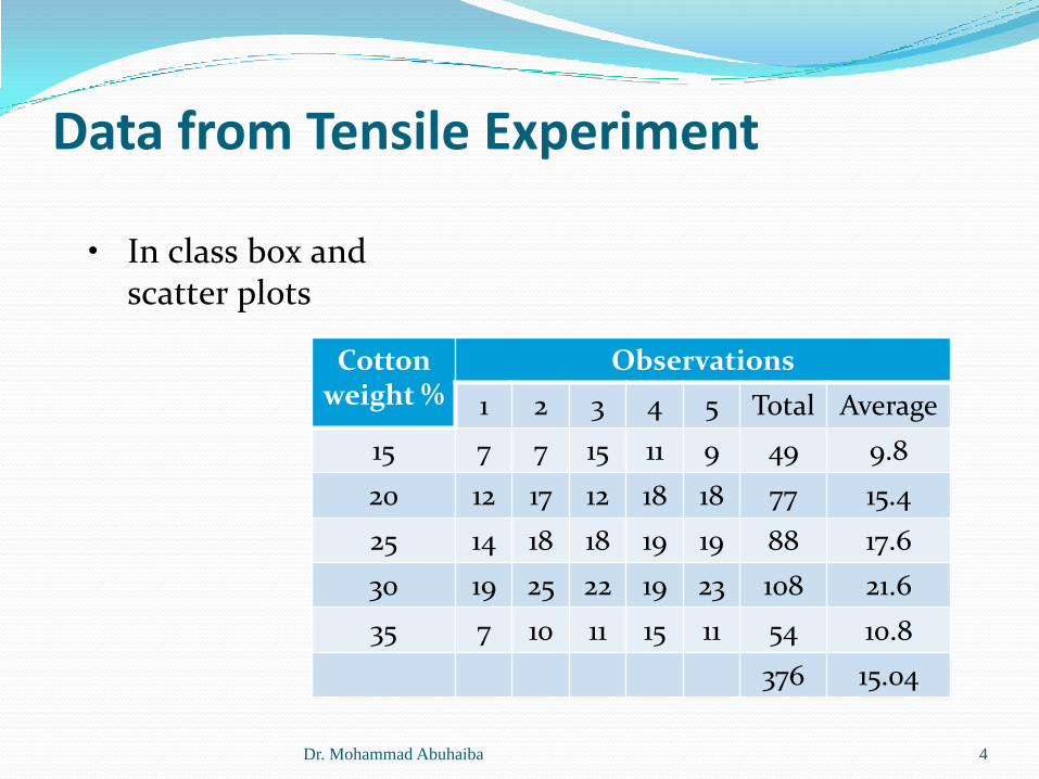
Data from Tensile Experiment

Cotton weight %

Observations

1 2 3 4 5 Total Average

15 7 7 15 11 9 49 9.8

20 12 17 12 18 18 77 15.4

25 14 18 18 19 19 88 17.6

30 19 25 22 19 23 108 21.6

35 7 10 11 15 11 54 10.8

376 15.04


• In class box and scatter plots

Graphical Representation

We strongly suspect that:

1. Cotton content affects tensile strength

2. Around 30% cotton results in max strength

The t-test is not the best solution for this problem because it would lead to considerable distortion in type I error.

Example


The Analysis of Variance

In general, there will be a levels of the factor, or a treatments, and n replicates of the experiment, run in random order… a completely randomized design (CRD)

N = an total runs

We consider the fixed effects case

Objective is to test hypotheses about the equality of the a treatment means


Models for the Data

There are several ways to write a model for the data:


is called the effects model

Let , then

is called the means model

ij i ij

i i

ij i ij

y

y

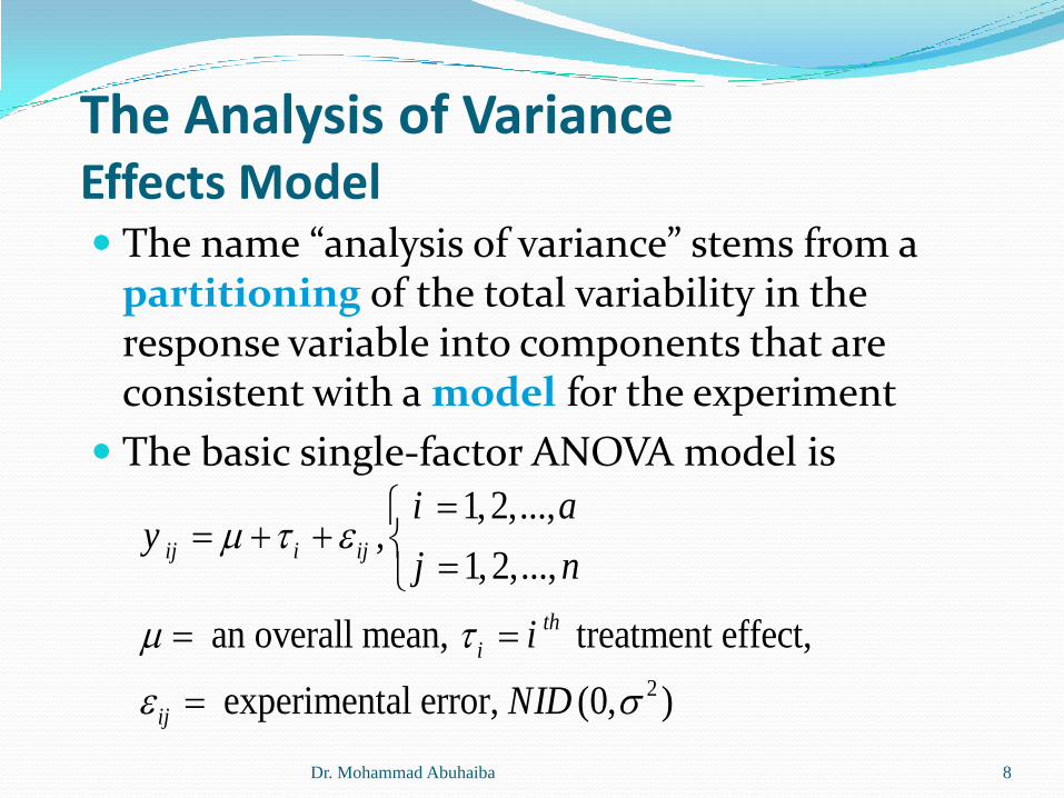
The Analysis of VarianceEffects Model The name “analysis of variance” stems from a

partitioning of the total variability in the response variable into components that are consistent with a model for the experiment

The basic single-factor ANOVA model is


2

1,2,...,,

1,2,...,

an overall mean, treatment effect,

experimental error, (0, )

ij i ij

th

i

ij

i ay

j n

i

NID

The Analysis of VarianceEffects Model

For hypothesis testing, the model errors are assumed to be normally and independently distributed random variables with mean zero and variance 2.

The variance 2 is assumed to be constant for all levels


2,ij iy N

THE ANALYSIS OF VARIANCEFixed Effects Model

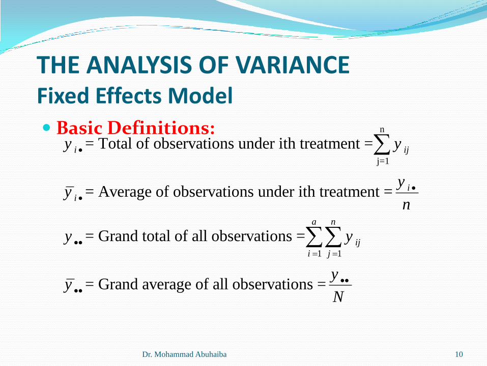
Basic Definitions:


n

j=1

1 1

= Total of observations under ith treatment =

= Average of observations under ith treatment =

= Grand total of all observations =

= Grand average of all observations

i ij

ii

a n

ij

i j

y y

yy

n

y y

y

=y

N

THE ANALYSIS OF VARIANCEFixed Effects Model

Hypothesises:

Another way to write the above hypothesis is in terms of treatment effects i:


1 2

1

1

1

: ...

: for at least one pair (i,j)

, , 0

o a

i j

a

i ai

i i i

i

H

H

a

1 2

1

: ... 0

: 0 for at least one i

o a

i

H

H

THE ANALYSIS OF VARIANCEFixed Effects Model – Total Sum of Squares

Total variability is measured by total sum of squares:

The basic ANOVA partitioning is:


2

..

1 1

( )a n

T ij

i j

SS y y

2 2

.. . .. .

1 1 1 1

2 2

. .. .

1 1 1

( ) [( ) ( )]

( ) ( )

a n a n

T ij i ij i

i j i j

a a n

i ij i Treatments E

i i j

SS y y y y y y

n y y y y SS SS

THE ANALYSIS OF VARIANCEFixed Effects Model – Total Sum of Squares

SSTreatments: sum of squares of differences between treatment averages and grand average.

It is a measure of differences between treatment means.

It has (a-1) DOF

SSE: sum of squares of differences of observations within treatments from the treatment average.

It is due to random error.

It has (N-a) DOF.



A large value of SSTreatments reflects large differences in treatment means

A small value of SSTreatments likely indicates no differences in treatment means

Formal statistical hypotheses are:


T Treatments ESS SS SS

0 1 2

1

:

: At least one mean is different

aH

H


While sums of squares cannot be directly compared to test the hypothesis of equal means, mean squares can be compared.

A mean square is a sum of squares divided by its degrees of freedom:

If the treatment means are equal, the treatment and error mean squares will be (theoretically) equal.

If treatment means differ, the treatment mean square will be larger than the error mean square.


1 1 ( 1)

,1 ( 1)

Total Treatments Error

Treatments ETreatments E

DOF DOF DOF

an a a n

SS SSMS MS

a a n


E(MSE) = 2

If there are no differences in treatment means (i =0), then E(MStreatments) = 2

If treatment means do differ, the expected value of treatment mean squares is greater than 2


2

2 1

1

a

i

iTreatments

n

E MSa


Test Statistic:


/( 1)

/( )

Treatments Treatmentso

E E

SS a MSF

SS N a MS

22

1 1

22

1

1

a n

T ij

i j

a

Treatments i

i

E T Treatments

ySS y

N

ySS y

n N

SS SS SS


The reference distribution for F0 is the Fa-1, a(n-1) distribution

Reject the null hypothesis (equal treatment means) if


0 , 1, ( 1)a a nF F

ANOVA TableExample 3-1: The tensile test experiment


Sum of squares DOF Mean Square Fo P-value

Cotton weight % 475.76 4 118.94 Fo = 14.76 <0.01

Error 161.2 20 8.06

Total 636.96 24

Cotton weight %

Observations

1 2 3 4 5 Total Average

15 7 7 15 11 9 49 9.8

20 12 17 12 18 18 77 15.4

25 14 18 18 19 19 88 17.6

30 19 25 22 19 23 108 21.6

35 7 10 11 15 11 54 10.8

376 15.04


The Reference Distribution

Coding the Observations

Example 3.2

Subtracting a constant from the original data does not change the sum of squares.

Multiply the observations in the original data does not change the F ratio


Estimation of the Model Parameters A 100(1-)% confidence interval on the ith treatment

mean, i:

A 100(1-)% confidence interval on the difference in any treatment means:

Example 3-3


/ 2, / 2,E E

i N a i i N a

MS MSy t y t

n n

/ 2, / 2,

2 2E Ei j N a i j i j N a

MS MSy y t y y t

n n

Unbalanced Data

The number of observations taken within each treatment may be different

Let ni observations be taken under treatment I, i=1,2,…,a:


22

1 1

2 2

1

1

a ni

T ij

i j

ai

Treatments

i i

a

i

i

ySS y

N

y ySS

n N

N n

Model Adequacy Checking in ANOVA

The use of partitioning to test for no differences in treatment means requires the satisfaction of the following assumptions:

Observations are adequetely described by the fixed effects model

Normality of errors

Constant unknown variance

Independence distributrion with zero mean

It is unwise to rely on ANOVA until the validity of these assumptions has been checked.


Model Adequacy Checking in ANOVA

Examination of residuals

If the model is adequate, residuals should be structureless: they should contain no obvious pattern

Residual plots are very useful


.

ˆij ij ij

ij i

e y y

y y

Model Adequacy CheckingNormal Probability Plot (NPP) of residuals

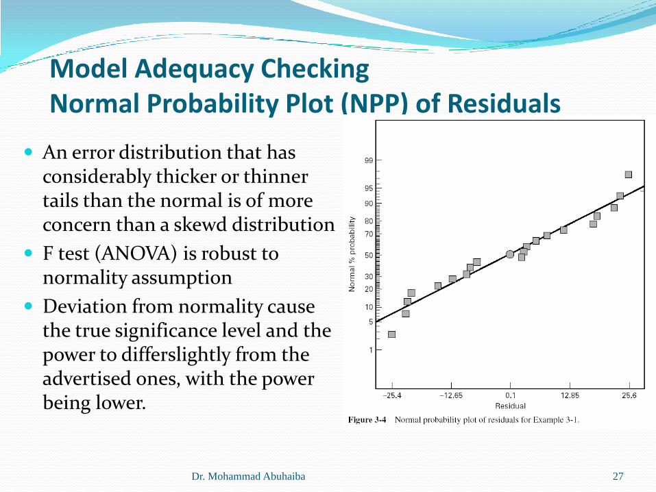
If the error distribution is normal, the plot will resemble a stright line.

Emphasis should be on the central values of the plot rather on the extremes

Table 3-6

Error distribution slightly skewed with longer right tail

The plot tend to bend down slightly on the left implying that the left tail of the error distribution is thinner than would be anticipated in a normal distributiom. The negative residuals are not as large as expected.


Model Adequacy CheckingNormal Probability Plot (NPP) of Residuals

An error distribution that has considerably thicker or thinner tails than the normal is of more concern than a skewd distribution

F test (ANOVA) is robust to normality assumption

Deviation from normality cause the true significance level and the power to differslightly from the advertised ones, with the power being lower.


Model Adequacy CheckingNPP of residuals - Outliers Outlier: a residual that is very much larger than any of the

others.

Causes: Mistake in calculations, data coding, or a typo

If this is not the cause, the experimental circumestances surrounding this run must be studied

If the outlying response is a particulary desirable value, the outlier may be more informative than the rest of the data

Not to reject an outlying observation unless we have solid ground for doing so.

We may end up with two analyses: one with outlier and one without


Model Adequacy CheckingNPP of residuals - Outliers Standardized residuals:

If ij are N(0,2), the Standardized residuals should be nearly normal with zero mean and unit variance

68% of Standardized residuals slould fall within the limits ±

95% of them within ±2

All of them within ±3

A residual bigger than 3 or 4 is a potential outlier

Example


ij

ij

E

ed

MS

Model Adequacy CheckingPlot of Residuals in Time Sequence

Non constant variance:

Sometimes the skill of the experimenter may change as the experiment progresses, or the process being studied may become more eratic.

This will often result in a change in the error variance over time, this condition often leads to a plot of resduals that exabits more spread at one end than at the other.

In our example ther is no evidence of any violation of independence or constant variance assumption


Model Adequacy CheckingPlot of Residuals vs Fitted Values

If the model is adequate and the assumptions are satisfied, the residuals should be unrelated to any other variable

Sometimes, Variance of observations increases as the magnitude of the observation increases

When Nonconstant variance case occurs, apply variance stablizing transformation


Model Adequacy CheckingPlot of Residuals vs Fitted Values- Transformation Experimenter knows theoritical distribution of

observations:

When there is no obvious transformation, experimental empirically seeks a transformation that equalizes variance regardless of value of mean

Transformation brings error distribution to normalDr. Mohammad Abuhaiba 32

Distribution Transformation

Poisson Square root

lognormal Logrithmic

Binomial Arcsin

* *

*

* 1

or 1

log

sin

ij ij ij ij

ij ij

ij ij

y y y y

y y

y y

Model Adequacy CheckingStatistical Test for Equality of VARIANCE-BARTLETT’S Test

Ho:

H1: above not true for at least one

Test statistic:

Q ia large when sample variances differ greatly, and is equal to zero when all variances are equal

Reject Ho when

When normality assumption is not valid, Bartlett’s test not used

Example 3-4Dr. Mohammoad Abuhaiba 33

2 2 2

1 2 ... a

2 2 2

1 10 10

1

2

1 1 2 1

1

2.3026 , log 1 log

11

1 1 , 3( 1)

a

p i i

i

a

i iai

i p

i

qx q N a S n S

c

n S

c n N a Sa N a

2 2

1 , 1ax x

Model Adequacy CheckingStatistical Test for Equality of VarianceModified Levene test

It is robust to departures from normality

Absolute deviation of observations yij in each treatment from treatment median:

If mean deviations are equal, variances in all treatments will be the same

Test statistic is the usual ANOVA F statistic applied to dij

Example 3-5

Dr. Mohammoad Abuhaiba 34

1,2,...,

1,2,...,ij ij i

i ad y y

j n

Model Adequacy CheckingEmpirical Selection of a Transformation

Suppose that the standard deviation of data is proportional to a power of the mean

Find a transformation that yields a constant variance.

Suppose that the transformation is a power of original data:

This yields

If we set l 1, the variance of transformed data is constant

Table 3-9: Variance stabilizing transformations

Apply transformation to Example 3-5

In practice: try several alternatives and observe the effect of each transformation on the plot of residuals vs predicted response.

Dr. Mohammoad Abuhaiba 35

*y y l

*

1

y

l

y

The Regression Model

Factors of an experiment:

1. Quantative: one whose levels can be associated with points on a numerical scale

2. Qualtative: levels can not arranged in order of magnitude

Model:

1. Quadratic:

2. Cubic:

The constant parameters are estimated by minimizing the sum of squares of errors


2

1 2oy x x 2 3

1 2 3oy x x x

The Regression Model


Post-ANOVA Comparison of Means

The analysis of variance tests the hypothesis of equal treatment means

Assume that residual analysis is satisfactory

If that hypothesis is rejected, we don’t know whichspecific means are different

Determining which specific means differ following an ANOVA is called the multiple comparisons problem

There are many ways to do this

Comparisons between treatment means are made in terms of:1. Treatment totals or

2. Treatment averages


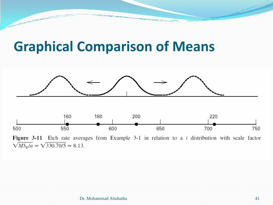
Graphical Comparison of MeansKnown Standard deviation of treatment average =

If all factor level means are identical, the observed sample means would behave as if they were a set of observations drawn at random from a normal distribution with mean and standard deviation

Visualize a normal distribution capable of being slid along an axis below which treatment means are plotted. If treatment means are all equal, there should be some position for

this distribution that makes it obvious that the treatment means were drawn from the same distribution. If this is not the case, treatment mean values that appear not to have been drawn from this distribution are associated with factor levels that produce different mean responses.


/ n

.iy

..y / n

Graphical Comparison of MeansunKnown Replace with from ANOVA and use a t-distribution with a

scale factor instead of the normal

Sketch of t-distribution in Figure 3-11:

Multiply abscissa t by scale factor

Plot this against ordinate of t at that point

The distribution can have an arbitrary origin


EMS

/EMS n

/ 8.06/5 1.27EMS n

Graphical Comparison of Means


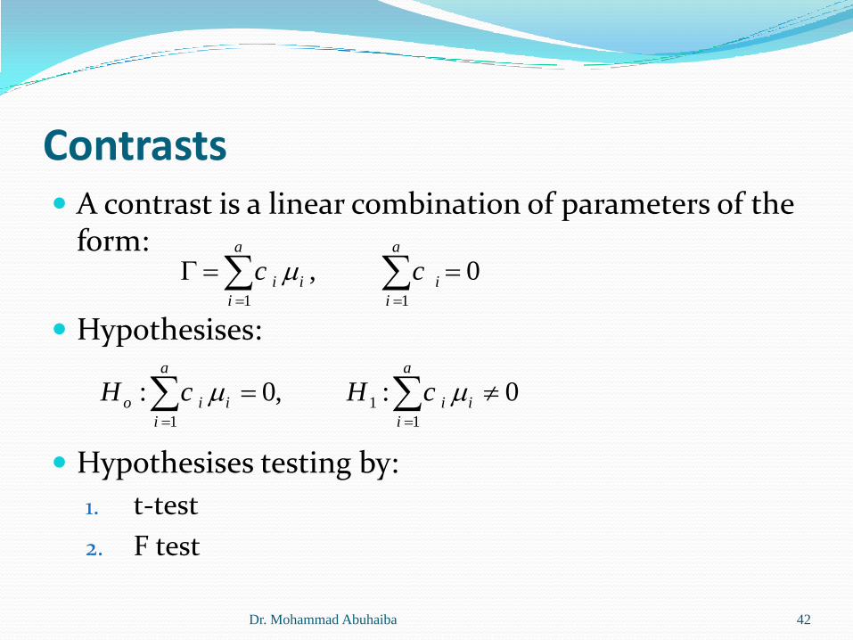
Contrasts A contrast is a linear combination of parameters of the

form:

Hypothesises:

Hypothesises testing by:

1. t-test

2. F test


1 1

, 0a a

i i i

i i

c c

1

1 1

: 0, : 0a a

o i i i i

i i

H c H c

Contrasts- Hypothesises testing t-test Contrast is in terms of treatment totals:

If Ho is true, then the ratio has N(0,1)

Test statistic

Ho is rejected if


2 2

.

1 1

, ( )a a

i i i

i i

C c y V C n c

.

1

2 2

1

a

i i

i

a

i

i

c y

n c

.

1

2

1

a

i i

io a

E i

i

c y

t

nMS c

/ 2,o N at t

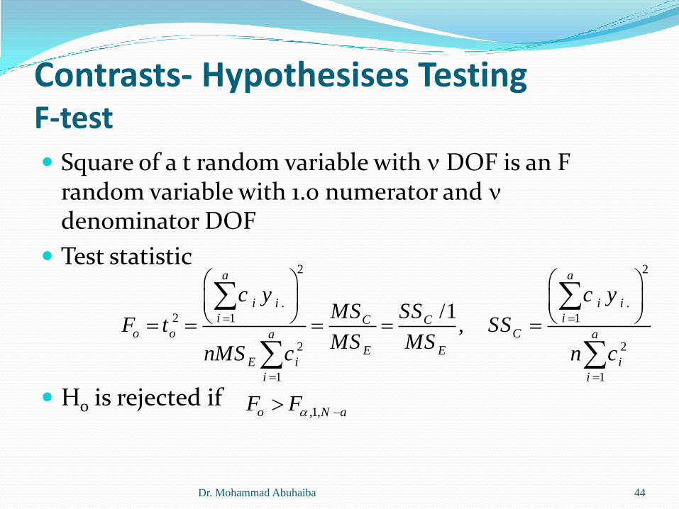
Contrasts- Hypothesises Testing F-test Square of a t random variable with n DOF is an F

random variable with 1.0 numerator and ndenominator DOF

Test statistic

Ho is rejected if


2 2

. .

2 1 1

2 2

1 1

/1,

a a

i i i i

i iC Co o Ca a

E EE i i

i i

c y c yMS SS

F t SSMS MS

nMS c n c

,1,o N aF F

Contrasts- Hypothesises Testing Confidence Interval Contrast in terms of treatment averages:

The 100(1-) confidence interval

If the confidence interval includes zero, we would be unable to reject Ho


2 2

. / 2, . / 2,

1 1 1 1

a a a aE E

i i N a i i i i i N a i

i i i i

MS MSc y t c c c y t c

n n

22

.

1 1 1

, , ( )a a a

i i i i i

i i i

c C c y V C cn

Contrasts- Hypothesises Testing Orthogonal Contrasts Two contrats with coefficients ci and di are orthogonal

if

Example 3-6


1

0a

i i

i

c d

Contrasts- Hypothesises Testing Sheffe’s Method for Comparing All Contrasts

A method for comparing any and all possible contrasts between treatment means.

Type I error is at most a for any of the possible comparisons

Set of m constrasts in the treatment means

Standard error

Example: P95Dr. Mohammad Abuhaiba 47

1 1 2 2

1 1. 2 2. .

... , 1,2,...,

...

u u u au a

u u u au a

c c c u m

C c y c y c y

2

1

/u

a

C E iu i

i

S MS c n

Contrasts- Hypothesises Testing Comparing pairs of Treatment Means – Tukey’s

Following ANOVA in which we have rejected the null hypothesis of equal treatment means

The overall significance level is exactly when sample sizes are equal and at most when sample sizes are unequal

Confidence level is 100(1- )% when sample sizes are equal and at least 100(1- )% when sample sizes are unequal

Two means are different if

100(1- )% confidence intervals:

Example 3-7Dr. Mohammad Abuhaiba 48

1: , :o i j i jH H

. . . ., ,E Ei j i j i j

MS MSy y q a f y y q a f

n n

. . , Ei j

MSy y T q a f

n

Contrasts- Hypothesises testing Comparing pairs of Treatment MeansFisher least Significant Difference (LSD) Means

Two means are significantly different if

Example 3-8


. . / 2,

1 1i j N a E

i j

y y LSD t MSn n

Contrasts- Hypothesises Testing Comparing pairs of Treatment MeansDuncan’s Multiple Range Test

Order treatment averages in ascending order

Standard error of each average:

Table VII: r(p,f), p=2,3,…,a

Rp =r(p,f) Syi.

Example 3-9


.

1

,

1/i

Ey h a

hi

i

MS aS n

nn

Contrasts- Hypothesises Testing Which Pairwise Comparison Method to Use?

No clear cut answer

LSD method is very effective test for detecting true differences in means if it is applied only after the F test in ANOVA is sginificant at 5%.

Good performance in detecting true differences with Duncan’s multiple range.


Choice of Sample Size1 2

= P(type I error) = P(reject Ho while Ho is true)

= P(type II error) = P(fail to reject Ho while Ho is false)

Power of the test = 1 – = P(reject Ho while Ho is false)

Choice of sample size is related to

Suppose that the means are not equal, d = 1 – 2.

Because Ho is not true, we are concerned about wrongly failing to reject Ho.

The probabilty of type II error depends on the true difference in means d.

Operating Characteristic Curve (OCC): graph of vs d for a particular sample size


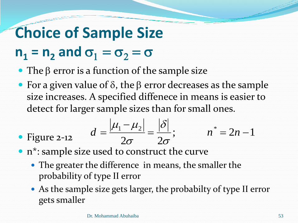
Choice of Sample Sizen1 = n2 and 1 2

The error is a function of the sample size

For a given value of d, the error decreases as the sample size increases. A specified diffenece in means is easier to detect for larger sample sizes than for small ones.

Figure 2-12

n*: sample size used to construct the curve

The greater the difference in means, the smaller the probability of type II error

As the sample size gets larger, the probabilty of type II error gets smaller


1 2 *; 2 12 2

d n n d

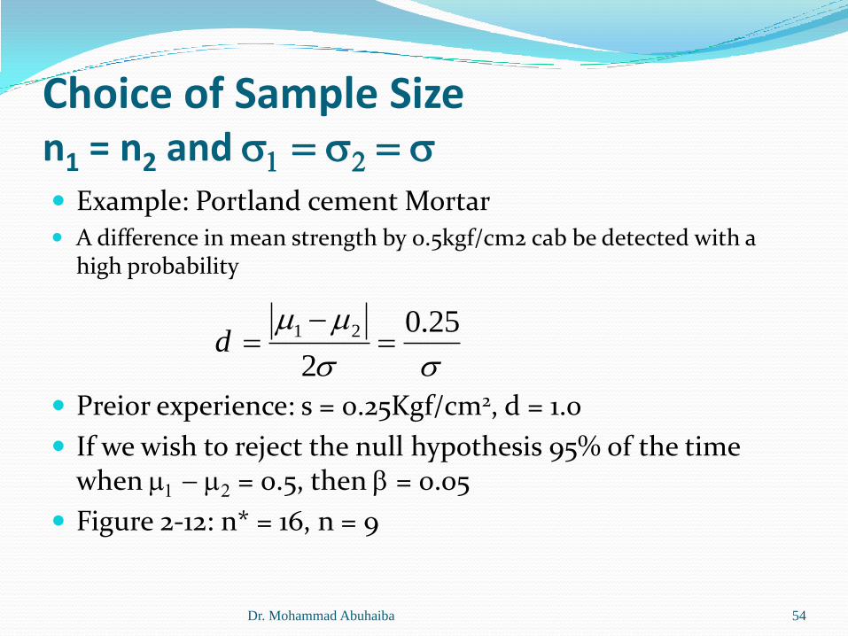
Choice of Sample Sizen1 = n2 and 1 2

Example: Portland cement Mortar A difference in mean strength by 0.5kgf/cm2 cab be detected with a

high probability

Preior experience: s = 0.25Kgf/cm2, d = 1.0

If we wish to reject the null hypothesis 95% of the time when 1 2 = 0.5, then = 0.05

Figure 2-12: n* = 16, n = 9


1 2 0.25

2d

Sample Size Determination

FAQ in designed experiments

Answer depends on lots of things; including:1. Type of experiment is being contemplated

2. how it will be conducted

3. resources,

4. desired sensitivity

Sensitivity refers to the difference in meansthat the experimenter wishes to detect

Generally, increasing the number of replications increases the sensitivity or it makes it easier to detect small differences in means Dr. Mohammad Abuhaiba 55

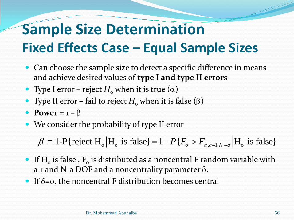
Sample Size DeterminationFixed Effects Case – Equal Sample Sizes Can choose the sample size to detect a specific difference in means

and achieve desired values of type I and type II errors

Type I error – reject H0 when it is true ()

Type II error – fail to reject H0 when it is false ()

Power = 1 –

We consider the probability of type II error

If Ho is false , Fo is distributed as a noncentral F random variable with a-1 and N-a DOF and a noncentrality parameter d.

If d=0, the noncentral F distribution becomes central


o o , 1, o = 1-P{reject H H is false} 1 { H is false}o a N aP F F

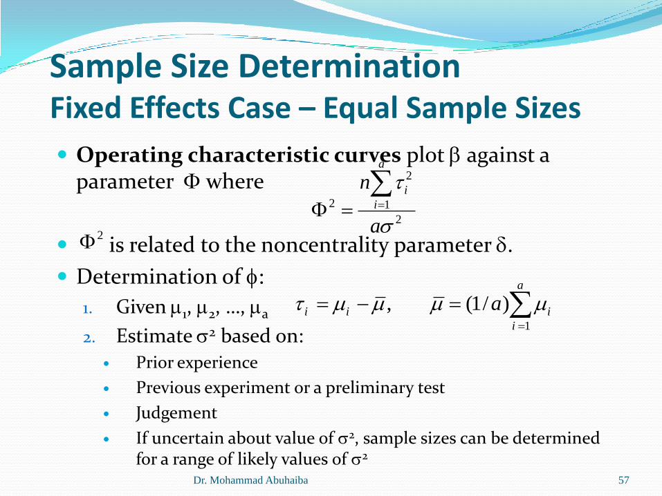
Sample Size DeterminationFixed Effects Case – Equal Sample Sizes

Operating characteristic curves plot against a parameter F where

is related to the noncentrality parameter d.

Determination of f:

1. Given 1, 2, …, a

2. Estimate 2 based on:

Prior experience

Previous experiment or a preliminary test

Judgement

If uncertain about value of 2, sample sizes can be determined for a range of likely values of 2


2

2 1

2

a

i

i

n

a

F

2F

1

, (1/ )a

i i i

i

a

Sample Size DeterminationFixed Effects Case---Use of OC Curves

The OC curves for the fixed effects model are in the Appendix, Table V, pg. 613

Example 3-11 A very common way to use these charts is to define a

difference in two means D of interest, then the minimum value of is

Typically work in term of the ratio of and try values of n until the desired power is achieved

Minitab will perform power and sample size calculations – see page 103

ExampleDr. Mohammad Abuhaiba 58

2F 22

22

nD

aF

/D

Sample Size DeterminationFixed Effects Case - Specify a Standard Deviation Increase

If the treatment means do not differ, the standard deviation of an observation chosen at random is .

If the treatment means are different, the standard deviation of an observation chosen at random is given by:

If we choose a %P for the increase in standard deviation of an observation beyond which we wish to reject the hypothesis that all treatment means are equal:

Example: P110Dr. Mohammad Abuhaiba 59

2 2

1

/a

i

i

a

2 2 2

1 1

/ /

1 , 1100 100/

a a

i i

i i

a aP P

nn

F


Power and Sample Size Calculations from Minitab

experiments with a single factor: the analysis of...

Documents