Expert Systems with Applications 42 (2015) 7549–7559

Contents lists available at ScienceDirect

Expert Systems with Applications

journal homepage: www.elsevier .com/locate /eswa

Data mining for fuzzy diagnosis systems in LTE networks

http://dx.doi.org/10.1016/j.eswa.2015.05.0310957-4174/� 2015 The Authors. Published by Elsevier Ltd.This is an open access article under the CC BY-NC-ND license (http://creativecommons.org/licenses/by-nc-nd/4.0/).

⇑ Corresponding author.E-mail addresses: emil@uma.es (E.J. Khatib), rbarco@uma.es (R. Barco), aga@ic.

uma.es (A. Gómez-Andrades), pabloml@ic.uma.es (P. Muñoz), inmaculada.serrano@ericsson.com (I. Serrano).

Emil J. Khatib a, Raquel Barco a,⇑, Ana Gómez-Andrades a, Pablo Muñoz a, Inmaculada Serrano b

a Universidad de Málaga, Communications Engineering Dept., Málaga, Spainb Ericsson, PBO RA Continuous Analysis, Spain

a r t i c l e i n f o

Article history:Available online 1 June 2015

Keywords:Self-healingSelf-Organizing NetworksLTEData miningData driven learningSupervised learningFault managementFuzzy systemsBig Data

a b s t r a c t

The recent developments in cellular networks, along with the increase in services, users and the demandof high quality have raised the Operational Expenditure (OPEX). Self-Organizing Networks (SON) are thesolution to reduce these costs. Within SON, self-healing is the functionality that aims to automaticallysolve problems in the radio access network, at the same time reducing the downtime and the impacton the user experience. Self-healing comprises four main functions: fault detection, root cause analysis,fault compensation and recovery. To perform the root cause analysis (also known as diagnosis),Knowledge-Based Systems (KBS) are commonly used, such as fuzzy logic. In this paper, a novel methodfor extracting the Knowledge Base for a KBS from solved troubleshooting cases is proposed. This methodis based on data mining techniques as opposed to the manual techniques currently used. The data miningproblem of extracting knowledge out of LTE troubleshooting information can be considered a Big Dataproblem. Therefore, the proposed method has been designed so it can be easily scaled up to process alarge volume of data with relatively low resources, as opposed to other existing algorithms. Tests showthe feasibility and good results obtained by the diagnosis system created by the proposed methodology inLTE networks.� 2015 The Authors. Published by Elsevier Ltd. This is an open access article under the CC BY-NC-ND license

(http://creativecommons.org/licenses/by-nc-nd/4.0/).

1. Introduction

In recent years, mobile communications have grown both intraffic volume and offered services. This has increased the expecta-tions for quality of service. In this scenario, service providers arepressed to increase their competitiveness, and therefore toincrease quality and reduce costs in the maintenance of their net-works. This task can only be achieved by increasing the degree ofautomation of the network. The Next Generation MobileNetworks (NGMN) Alliance (NGMN, 2006) defined Self-OrganizingNetworks (SON) as a set of principles and concepts to add automa-tion to mobile networks. Recently, these ideas were applied to LongTerm Evolution (LTE) networks by the 3rd Generation PartnershipProject (3GPP) (3GPP, 2012) in the form of use cases and specificSON functionalities. The SON concept is composed by three fields:self-configuration, self-optimization and self-healing. This paper isfocused on self-healing, which includes all the functionalitytargeted towards automating troubleshooting in the radio accessnetwork (RAN). Currently, the task of RAN troubleshooting is

manually done, so the ability of automating it is a great competi-tive advantage for operators. The benefits of self-healing arenumerous, since it will offload troubleshooting experts of repeti-tive maintenance work and let them focus on improving the net-work. It also reduces the downtime of the network, thereforeincreasing the quality perceived by the users.

Self-healing is composed of four main tasks: fault detection,root cause analysis (diagnosis), compensation and fault recovery(Barco, Lázaro, & Muñoz, 2012). Currently there are no commercialimplementations of these functions, although some research efforthas been recently made.

The reason of this shortage of implementations, according tothe COMMUNE project (COMMUNE, 2012) is the high degree ofuncertainty in diagnosis in the RAN of mobile networks. TheCOMMUNE project uses a case based reasoning algorithm(Szilagyi & Novaczki, 2012) where a vector of PerformanceIndicators (PIs) is compared against a database of known problems.The cause will be the same as the case of the nearest storedproblem.

In Barco, Díez, Wille, and Lázaro (2009) a Bayesian Network(BN) is used to do the diagnosis. To implement the system, it isrequired that an expert sets the parameters of the BN, so aKnowledge Acquisition Tool is also presented in Barco, Lázaro,Wille, Díez, and Patel (2009).

7550 E.J. Khatib et al. / Expert Systems with Applications 42 (2015) 7549–7559

The UniverSelf project (Univerself, 2012) combines BNs withcase-based reasoning (Bennacer, Ciavaglia, Chibani, Amirat, &Mellouk, 2012; Hounkonnou & Fabre, 2012) for the diagnosis pro-cess. Apart from the previous references in diagnosis, research inself-healing has also been extended to detection (Asghar,Hamalainen, & Ristaniemi, 2012; Barreto, Mota, Souza, Frota, &Aguayo, 2005) and compensation (Eckhardt et al., 2011; Razavi,2012), which are out of the scope of this paper.

This paper proposes a method for learning troubleshootingrules for diagnosis methods based on Fuzzy Logic Controllers(FLCs) (Lee, 1990). FLCs use fuzzy logic (Zadeh, 1965) to assignfuzzy values to numerical variables, and by applying fuzzy rules,they obtain the value of an output variable (e.g. a parametervalue) or a given action. FLCs have been used for diagnosis inother fields, such as industrial processes (Serdio, Lughofer,Pichler, Buchegger, & Efendic, 2014), machinery operation(Serdio et al., 2014; Lughofer & Guardiola, 2008) or medicaldiagnosis(Innocent, John, & Garibaldi, 2004). Although FLCs havebeen used in mobile networks for self-optimization (Muñoz,Barco, & de la Bandera, 2013a; Muñoz, Barco, & de la Bandera,2013b), there are no previous references proposing its applicationto self-healing.

The implementation of the diagnosis process is done byKnowledge-Based Systems (KBS) (Akerkar & Sajja, 2010;Triantaphyllou & Felici, 2006) such as BNs and FLCs. KBS are com-posed of two main parts: the Inference Engine (IE) and theKnowledge Base (KB). This separation permits the algorithm tobe used in a variety of situations by changing only the KB. Still,the construction of the KB, or Knowledge Acquisition (KA)(Triantaphyllou & Felici, 2006; Maier, 2007) is a major researchtopic. This is where the previous KA proposals in literature fordiagnosis in wireless networks fail to deliver convincing results.The KA process involves the troubleshooting experts in a timeconsuming process (Studer, Benjamins, & Fensel, 1998;Ruiz-Aviles, Luna-Ramírez, Toril, & Ruiz, 2012; Chung, Chang, &Wang, 2012; Barco et al., 2009). It is based on the fact that theknowledge is contained in the experience of the expert. An alter-native approach (Triantaphyllou & Felici, 2006) considers that theknowledge applied by the experts in the troubleshooting processwill also be contained in its results. Every pair composed of thePIs and the fault cause and/or action(s) to be taken provided bythe expert contains information about what aspects are observedby the expert and how they are related to each other. Therefore, aproblem database (Hatamura, Ilno, Tsuchlya, & Hamaguchi, 2003)can be created, where each problem is saved along with itsdiagnosis; and this database will hold the expert’s knowledgeimplicitly.

Data mining (DM) consists of the discovery of patterns in largedata sets through the application of specific algorithms(Kantardzic, 2011; Witten, Frank, & Mark, 2011; Han, Kamber, &Pei, 2012). The result of DM is a model of the studied system.DM is used to process information from sensor networks(Papadimitriou, Brockwell, & Faloutsos, 2003), in scientific datacollection (Ball & Brunner, 2010) or computer science (Ektefa,Memar, Sidi, & Affendey, 2010). DM is also used in commercialapplications to find marketing trends (Linoff & Berry, 2011).Modern data collection and monitoring systems produce largeamounts of data containing valuable knowledge, but due to thehuge amount of information, this knowledge is hidden and needsto be extracted and easily visualized. In fact, the traditional DMtechniques are often insufficient or ineffective for the large amountof available data. This leads to the development of Big Data tech-niques (Russom, 2011), which deal with databases that have spe-cial requirements due to one or more of the following factors,known as the 3 Vs of Big Data:

� Volume: the amount of data generated may require new trans-mission, storage and processing techniques. In the case ofmobile networks, data is produced by each network element(e.g. eNodeB) over all the network, but also by each connectedterminal.� Velocity: usually there are constraints on the time when the

analysis results must be available, so that the information canbe used in real time. In mobile networks, part of the data is pro-duced in streams, that is, continuously as new events happenwhile the users access the services. In order to reduce process-ing times, heavy parallelization is very often the best solution.� Variety: data is not always normalized and clearly structured.

Also, formats vary depending on the nature of the data andthe element that produces it.

In this work, a DM algorithm for obtaining fuzzy rules in the ‘‘if. . . then . . .’’ form for the diagnosis of the RAN of LTE networks isproposed, which relates certain behaviors in the PIs of a sector ata given time to the possible problem that is present in it. The rulesreflect the knowledge of the experts that is implicitly contained inthe results of their work (a database containing the solvedproblems). Other learning algorithms have been proposed for fuzzyrules in other fields, but none of them have been adapted tomobile communication networks (Wang & Mendel, 1992;Cordon, Herrera, & Villar, 2011; Lughofer & Kindermann, 2010;Pratama, Anavatti, Angelov, & Lughofer, 2014; Chen, 2013;Babuska, 1998). This algorithm has been designed to be easilyparallelizable in order to fit the velocity requirements describedearlier and to minimize the memory footprint so a large volumeof data can be processed.

The remaining of this paper is organized as follows. In Section 2the traditional processes of troubleshooting is presented, alongwith the use of KBS for automating it. In Section 3 the proposedDM algorithm for automating the KA process is presented.Afterwards, in Section 4, the system is tested and its performanceis compared with another learning algorithm. Finally, the conclu-sions are discussed in Section 5.

2. Problem formulation

2.1. Troubleshooting in LTE networks

The process of troubleshooting is made up of four main tasks:

� Detection: determining that there is a problem in the networkand isolating its origin, that is, the sectors that are degradingthe performance of the whole network.� Compensation: reconfiguration of the neighboring sectors to

cover the affected users.� Diagnosis: determining the cause of the problem.� Recovery: actions to restore the affected sector to a normal

state.

This process is usually manually done. Experts monitor areduced set of Key Performance Indicators (KPIs), aggregated overthe whole network. KPIs are composite variables that contain theinformation of several low-level PIs and reflect the general behav-ior of the sector. When one (or several) of those KPIs is degraded(e.g. it is lower than a certain threshold), a list of the worst offend-ers is obtained, showing the sectors that more strongly degrade theKPI. Those sectors are then diagnosed by observing further symp-toms (i.e. abnormal values of PIs and other low-level metrics, suchas counters, measurements and alarms). The relations among thesesymptoms, described by heuristic ‘‘if . . . then . . .’’ rules, determine

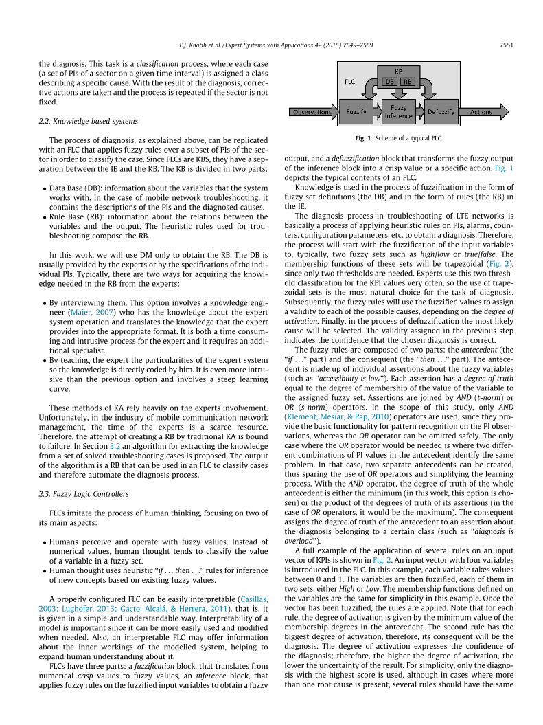
Fig. 1. Scheme of a typical FLC.

E.J. Khatib et al. / Expert Systems with Applications 42 (2015) 7549–7559 7551

the diagnosis. This task is a classification process, where each case(a set of PIs of a sector on a given time interval) is assigned a classdescribing a specific cause. With the result of the diagnosis, correc-tive actions are taken and the process is repeated if the sector is notfixed.

2.2. Knowledge based systems

The process of diagnosis, as explained above, can be replicatedwith an FLC that applies fuzzy rules over a subset of PIs of the sec-tor in order to classify the case. Since FLCs are KBS, they have a sep-aration between the IE and the KB. The KB is divided in two parts:

� Data Base (DB): information about the variables that the systemworks with. In the case of mobile network troubleshooting, itcontains the descriptions of the PIs and the diagnosed causes.� Rule Base (RB): information about the relations between the

variables and the output. The heuristic rules used for trou-bleshooting compose the RB.

In this work, we will use DM only to obtain the RB. The DB isusually provided by the experts or by the specifications of the indi-vidual PIs. Typically, there are two ways for acquiring the knowl-edge needed in the RB from the experts:

� By interviewing them. This option involves a knowledge engi-neer (Maier, 2007) who has the knowledge about the expertsystem operation and translates the knowledge that the expertprovides into the appropriate format. It is both a time consum-ing and intrusive process for the expert and it requires an addi-tional specialist.� By teaching the expert the particularities of the expert system

so the knowledge is directly coded by him. It is even more intru-sive than the previous option and involves a steep learningcurve.

These methods of KA rely heavily on the experts involvement.Unfortunately, in the industry of mobile communication networkmanagement, the time of the experts is a scarce resource.Therefore, the attempt of creating a RB by traditional KA is boundto failure. In Section 3.2 an algorithm for extracting the knowledgefrom a set of solved troubleshooting cases is proposed. The outputof the algorithm is a RB that can be used in an FLC to classify casesand therefore automate the diagnosis process.

2.3. Fuzzy Logic Controllers

FLCs imitate the process of human thinking, focusing on two ofits main aspects:

� Humans perceive and operate with fuzzy values. Instead ofnumerical values, human thought tends to classify the valueof a variable in a fuzzy set.� Human thought uses heuristic ‘‘if . . . then . . .’’ rules for inference

of new concepts based on existing fuzzy values.

A properly configured FLC can be easily interpretable (Casillas,2003; Lughofer, 2013; Gacto, Alcalá, & Herrera, 2011), that is, itis given in a simple and understandable way. Interpretability of amodel is important since it can be more easily used and modifiedwhen needed. Also, an interpretable FLC may offer informationabout the inner workings of the modelled system, helping toexpand human understanding about it.

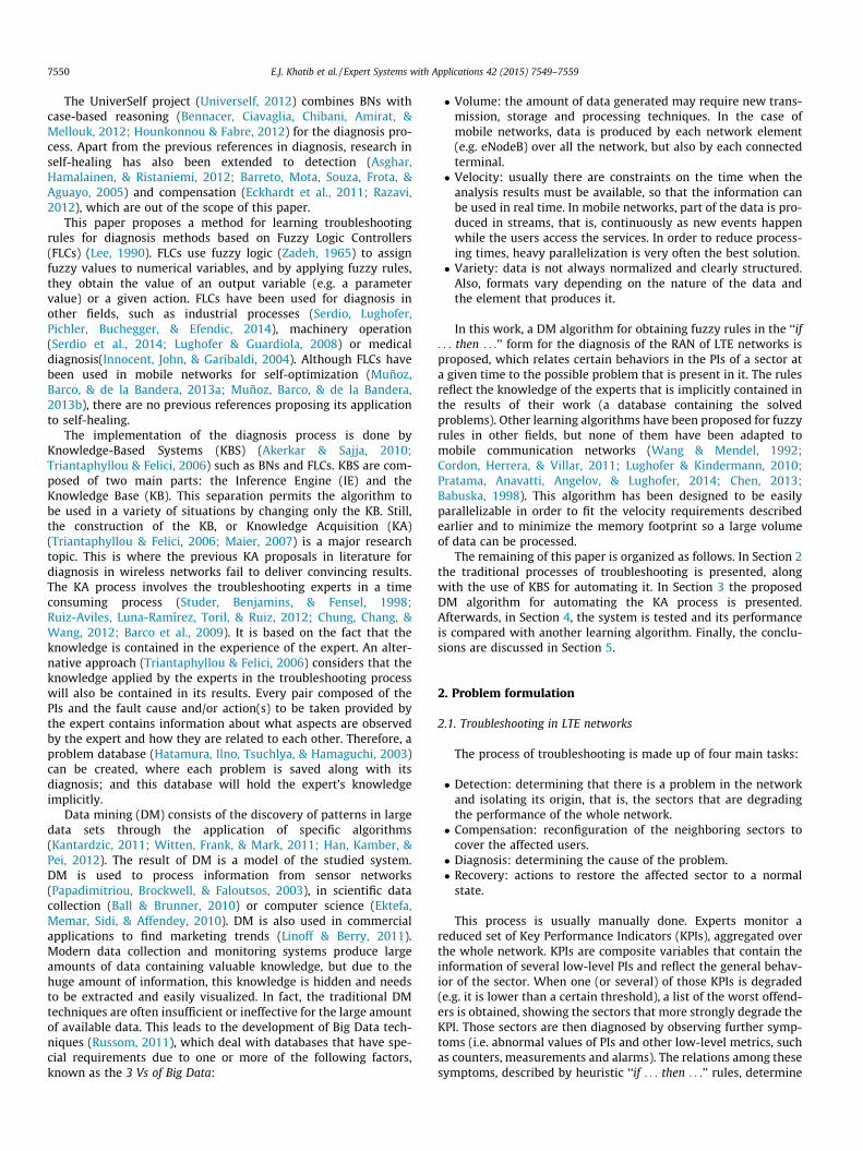
FLCs have three parts; a fuzzification block, that translates fromnumerical crisp values to fuzzy values, an inference block, thatapplies fuzzy rules on the fuzzified input variables to obtain a fuzzy

output, and a defuzzification block that transforms the fuzzy outputof the inference block into a crisp value or a specific action. Fig. 1depicts the typical contents of an FLC.

Knowledge is used in the process of fuzzification in the form offuzzy set definitions (the DB) and in the form of rules (the RB) inthe IE.

The diagnosis process in troubleshooting of LTE networks isbasically a process of applying heuristic rules on PIs, alarms, coun-ters, configuration parameters, etc. to obtain a diagnosis. Therefore,the process will start with the fuzzification of the input variablesto, typically, two fuzzy sets such as high/low or true/false. Themembership functions of these sets will be trapezoidal (Fig. 2),since only two thresholds are needed. Experts use this two thresh-old classification for the KPI values very often, so the use of trape-zoidal sets is the most natural choice for the task of diagnosis.Subsequently, the fuzzy rules will use the fuzzified values to assigna validity to each of the possible causes, depending on the degree ofactivation. Finally, in the process of defuzzification the most likelycause will be selected. The validity assigned in the previous stepindicates the confidence that the chosen diagnosis is correct.

The fuzzy rules are composed of two parts: the antecedent (the‘‘if . . .’’ part) and the consequent (the ‘‘then . . .’’ part). The antece-dent is made up of individual assertions about the fuzzy variables(such as ‘‘accessibility is low’’). Each assertion has a degree of truthequal to the degree of membership of the value of the variable tothe assigned fuzzy set. Assertions are joined by AND (t-norm) orOR (s-norm) operators. In the scope of this study, only AND(Klement, Mesiar, & Pap, 2010) operators are used, since they pro-vide the basic functionality for pattern recognition on the PI obser-vations, whereas the OR operator can be omitted safely. The onlycase where the OR operator would be needed is where two differ-ent combinations of PI values in the antecedent identify the sameproblem. In that case, two separate antecedents can be created,thus sparing the use of OR operators and simplifying the learningprocess. With the AND operator, the degree of truth of the wholeantecedent is either the minimum (in this work, this option is cho-sen) or the product of the degrees of truth of its assertions (in thecase of OR operators, it would be the maximum). The consequentassigns the degree of truth of the antecedent to an assertion aboutthe diagnosis belonging to a certain class (such as ‘‘diagnosis isoverload’’).

A full example of the application of several rules on an inputvector of KPIs is shown in Fig. 2. An input vector with four variablesis introduced in the FLC. In this example, each variable takes valuesbetween 0 and 1. The variables are then fuzzified, each of them intwo sets, either High or Low. The membership functions defined onthe variables are the same for simplicity in this example. Once thevector has been fuzzified, the rules are applied. Note that for eachrule, the degree of activation is given by the minimum value of themembership degrees in the antecedent. The second rule has thebiggest degree of activation, therefore, its consequent will be thediagnosis. The degree of activation expresses the confidence ofthe diagnosis; therefore, the higher the degree of activation, thelower the uncertainty of the result. For simplicity, only the diagno-sis with the highest score is used, although in cases where morethan one root cause is present, several rules should have the same

Fig. 2. Rule application process.

7552 E.J. Khatib et al. / Expert Systems with Applications 42 (2015) 7549–7559

score. Even if only one diagnosis has the maximum score, it is stilluseful to provide a list of all the activated diagnoses ordered bydescending score so the experts have a broader picture of the stateof the sector. Another alternative to the scoring approach used inthis study is weighted voting (Lughofer & Buchtala, 2013), whereeach diagnosis is compared individually with each of the otherdiagnoses through a single rule with two possible outcomes.Each rule will then vote for one of two possible diagnoses.

3. Data mining in LTE troubleshooting databases

3.1. Data mining

DM is the process that extracts a model out of a data set byexploring the underlying patterns. Knowledge Discovery andData Mining (KDD) (Maimon & Last, 2001) is the larger processextending from the collection of the relevant data saved into a database to the interpretation of the knowledge contained in it.

The DM algorithm proposed in this work obtains fuzzy rulesfrom a set of solved cases (training set). These rules will take aset of PIs as input and produce a diagnosis (they will classify thecases). Therefore, the DM algorithm will solve a classification prob-lem. The learned model (the fuzzy rule set) is a classifier. Ideally, thelearned rules will be similar to those used by the experts. Eachentry in the training set (case) is a tuple formed by an n-dimen-sional attribute vector (in this case, the values of PIs) and a classlabel that identifies the class to which the case belongs (in thisstudy, this is the diagnosis). Since the training set contains the classlabel, the DM algorithm is a supervised learning algorithm.

To obtain the required vectors, a previous process of data reduc-tion (Khatib, Barco, Serrano, & Muñoz, 2014) must be carried out.The data extracted from the network will be a set oftime-dependent arrays representing time series for each PI. Thistime series covers the time interval where the problem occurred,but also the surrounding time intervals where the fault did notshow up in the data. Therefore, two steps must be achieved:

� Isolating the problem in time, so the data reflects only the influ-ence of the root cause.� Converting the set of time series to a vector with one value per

PI. Once the problem is isolated, this can be done with an aver-age value of the PI for the affected time interval.

The issue of data reduction is out of the scope of this article, butit is a necessary prior step to the data driven learning process.

3.2. Data driven learning in troubleshooting databases

In this study, a novel supervised data driven learning algorithmfor wireless networks based on the WM (Wang & Mendel, 1992)method is described. It introduces some modifications in order tobetter adapt to the obtention of the rules used in troubleshootingof LTE networks. The WM method is a well known algorithm thatcan easily be parallelized since the creation of new rules from thedata is independent from the creation of previous rules. Therefore,the data can be divided among several processes arbitrarily with-out loss of information. Another advantage of the WM method isthat it is deterministic, that is, the results of two equal training setsare always equal, independently from the order that the data isprovided or how it is divided among parallel processes. Otherlearning algorithms have been proposed (Cordón, Herrera,Gomide, Hoffmann, & Magdalena, 2001; Khatib, Barco,Góomez-Andrades, & Serrano, in press; Angelov, Lughofer, &Zhou, 2008; Ishibuchi & Nakashima, 2001), but the WM methodwas found the best for parallelization and for its deterministicbehavior, which helps understanding the results of the learningprocess.

The algorithm obtains the RB of an FLC from a training set com-

posed of labeled cases. The learning cases are tuples C ¼ ðk; dÞ com-

posed of a vector k ¼ fk1; k2 . . . kNg as the attribute vectorrepresenting the values of PIs PI ¼ fPI1; PI2 . . . PINg and a label d asthe class label among possible root causes RC ¼ fRC1;RC2 . . . RCMg.The algorithm has three consecutive steps:

E.J. Khatib et al. / Expert Systems with Applications 42 (2015) 7549–7559 7553

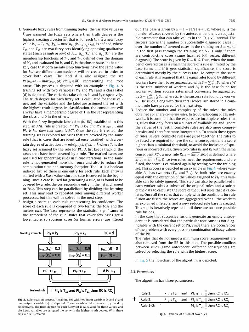
1. Generate fuzzy rules from training tuples: the variable values in

k are assigned the fuzzy sets where their truth degree is the

highest, creating a vector kF ; that is, for each kn 2 k a new fuzzyvalue kFn ¼ TnjlTn

ðknÞ ¼ maxðlT1nðknÞ;lT2n

ðknÞÞ is defined, whereT1n and T2n are two fuzzy sets identifying opposing qualitativestates (such as high or low) of PIn; lT1n

ðknÞ and lT2nðknÞ are the

membership functions of T1n and T2n defined over the domainof PIn and evaluated for kn and Tn is the chosen state. In the unli-kely case that both membership functions have the same valuefor kn, two different antecedents will be created, in order tocover both cases. The label d is also assigned the setRCjlRCðdÞ ¼ maxðlRCm

ðdÞÞ8RCm 2 RC representing the rootcause. This process is depicted with an example in Fig. 3. Atraining set with two variables (PI1 and PI2) and a class label(d) is depicted. The variables take values k1 and k2 respectively.The truth degree for each fuzzy set is calculated for these val-ues, and the variables and the label are assigned the set withthe highest truth degree. In classification, the consequent willalways have a membership degree of 1 in the set representingthe class and 0 in the others.

With the fuzzy linguistic labels R ¼ ðkF ;RCÞ established in thisstep, an AND rule is created: ‘‘if PI1 is kF1 and PI2 is kF2 . . . andPIN is kFN then root cause is RC’’. Once the rule is created, thetraining set is explored for cases that are covered by the samerule (that is, cases that are identical once fuzzified) with a cer-

tain degree of activation a ¼ minðlTnðknÞÞ8kn 2 k where Tn is the

fuzzy set assigned by the rule for PIn. A list keeps track of thecases that have been covered by a rule. The marked cases arenot used for generating rules in future iterations, so the samerule is not generated more than once and also to reduce thecomputation time and memory footprint. The list is a booleanindexed list, so there is one entry for each rule. Each entry isstarted with a False value, since no case is covered in the begin-ning. Once a case is used for generating a rule, or is found to becovered by a rule, the corresponding entry in the list is changedto True. This step can be parallelized by dividing the learningset. This may lead to repeated rules among different workerprocesses, but this will be solved in the next step.

2. Assign a score to each rule representing its confidence. Thescore of each rule is composed of two terms: the base and thesuccess rate. The base represents the statistical significance ofthe antecedent of the rule. Rules that cover few cases get alower score, so spurious cases (or human errors) are filtered

Fig. 3. Rule creation process. A training set with two input variables (x and y) andone output variable (z) is depicted. These variables take values x1; y1 and z1

respectively. The truth degree for each fuzzy set is calculated for these values, andthe input variables are assigned the set with the highest truth degree. With thesesets, a rule is created.

out. The base is given by B ¼ 1� ð1=ð1þ ancÞÞ, where nc is thenumber of cases covered by the antecedent and a is an adjusta-ble parameter that can take values in the ð0;þ1Þ interval. Thesuccess rate is the number of successfully diagnosed cases ns

over the number of covered cases in the training set S ¼ ns=nc.In the first pass through the training set, S < 1 only if thereare contradicting cases (same fuzzified KPI vector, differentdiagnosis). The score is given by D ¼ B � S. Thus, when the num-ber of covered cases is small, the score of a rule is limited by thebase term; and if it gets statistical significance, the score isdetermined mostly by the success rate. To compute the scoreof each rule, it is required that the equal rules found by different

workers have their bases aggregated with B ¼PW

w¼1Bw where Wis the total number of workers and Bw is the base found forworker w. Their success rates must conversely be aggregated

by S ¼PW

w¼1BwB Sw, where Sw is the success rate found by worker

w. The rules, along with their total scores, are stored in a com-mon rule base prepared for the next step.

3. Reduce the number and complexity of the rules: the rulesobtained so far are complete rules. In troubleshooting of LTE net-works, it is common that the experts use incomplete rules, thatis, rules that only focus on a subset of available PIs and ignorethe values of the rest. Incomplete rules are also more compre-hensive and therefore more interpretable. To obtain these typesof rules, several complete rules are fused together. The rules tobe fused are required to have the same consequent and a scorehigher than a minimal threshold, to avoid the inclusion of spu-rious or incorrect rules. Given two rules R1 and R2 with the same

consequent RCC , a new rule R1þ2 ¼ ðkF1þ2;RCCÞ is defined where

kF1þ2 ¼ kF1 \ kF2. Once two rules meet the requirements and arefused, the score is calculated again by testing over the trainingset. This process is depicted in an example in Fig. 4, where vari-able PI1 has two sets (T11 and T12). As both rules are exactlyequal with the exception of the values assigned to PI1, this vari-able can be safely ignored. This step can also be parallelized ifeach worker takes a subset of the original rules and a subsetof the data to calculate the score of the fused rules that it calcu-lates. Once all the rules that comply with the conditions for rulefusion are fused, the scores are aggregated over all the workersas explained in Step 2, and a new reduced rule base is created.This step is iteratively repeated until there are no more possiblerule fusions.In the case that successive fusions generate an empty antece-dent, it is considered that the particular root cause is not diag-nosable with the current set of PIs, since there are occurrencesof the problem with every possible combination of fuzzy valuesof the PIs.The rules that do not meet a minimum score requirement arealso removed from the RB in this step. The possible conflictsbetween rules (same antecedent, different consequents) aresolved by selecting the rule with the highest score.

In Fig. 5 the flowchart of the algorithm is depicted.

3.3. Parameters

The algorithm has three parameters:

Fig. 4. Example of fusion of two rules.

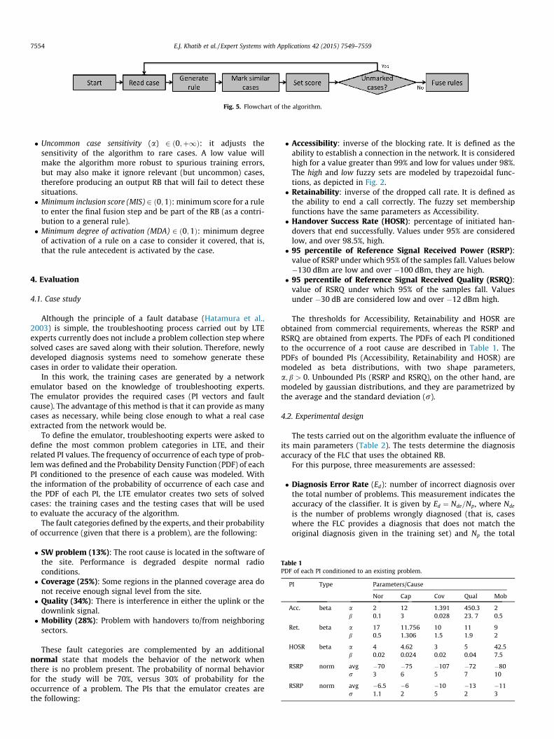
Fig. 5. Flowchart of the algorithm.

Table 1PDF of each PI conditioned to an existing problem.

PI Type Parameters/Cause

Nor Cap Cov Qual Mob

Acc. beta a 2 12 1.391 450.3 2b 0.1 3 0.028 23. 7 0.5

Ret. beta a 17 11.756 10 11 9b 0.5 1.306 1.5 1.9 2

HOSR beta a 4 4.62 3 5 42.5b 0.02 0.024 0.02 0.04 7.5

RSRP norm avg �70 �75 �107 �72 �80r 3 6 5 7 10

RSRP norm avg �6.5 �6 �10 �13 �11r 1.1 2 5 2 3

7554 E.J. Khatib et al. / Expert Systems with Applications 42 (2015) 7549–7559

� Uncommon case sensitivity (a) 2 ð0;þ1Þ: it adjusts thesensitivity of the algorithm to rare cases. A low value willmake the algorithm more robust to spurious training errors,but may also make it ignore relevant (but uncommon) cases,therefore producing an output RB that will fail to detect thesesituations.� Minimum inclusion score (MIS) 2 ð0;1Þ: minimum score for a rule

to enter the final fusion step and be part of the RB (as a contri-bution to a general rule).� Minimum degree of activation (MDA) 2 ð0;1Þ: minimum degree

of activation of a rule on a case to consider it covered, that is,that the rule antecedent is activated by the case.

4. Evaluation

4.1. Case study

Although the principle of a fault database (Hatamura et al.,2003) is simple, the troubleshooting process carried out by LTEexperts currently does not include a problem collection step wheresolved cases are saved along with their solution. Therefore, newlydeveloped diagnosis systems need to somehow generate thesecases in order to validate their operation.

In this work, the training cases are generated by a networkemulator based on the knowledge of troubleshooting experts.The emulator provides the required cases (PI vectors and faultcause). The advantage of this method is that it can provide as manycases as necessary, while being close enough to what a real caseextracted from the network would be.

To define the emulator, troubleshooting experts were asked todefine the most common problem categories in LTE, and theirrelated PI values. The frequency of occurrence of each type of prob-lem was defined and the Probability Density Function (PDF) of eachPI conditioned to the presence of each cause was modeled. Withthe information of the probability of occurrence of each case andthe PDF of each PI, the LTE emulator creates two sets of solvedcases: the training cases and the testing cases that will be usedto evaluate the accuracy of the algorithm.

The fault categories defined by the experts, and their probabilityof occurrence (given that there is a problem), are the following:

� SW problem (13%): The root cause is located in the software ofthe site. Performance is degraded despite normal radioconditions.� Coverage (25%): Some regions in the planned coverage area do

not receive enough signal level from the site.� Quality (34%): There is interference in either the uplink or the

downlink signal.� Mobility (28%): Problem with handovers to/from neighboring

sectors.

These fault categories are complemented by an additionalnormal state that models the behavior of the network whenthere is no problem present. The probability of normal behaviorfor the study will be 70%, versus 30% of probability for theoccurrence of a problem. The PIs that the emulator creates arethe following:

� Accessibility: inverse of the blocking rate. It is defined as theability to establish a connection in the network. It is consideredhigh for a value greater than 99% and low for values under 98%.The high and low fuzzy sets are modeled by trapezoidal func-tions, as depicted in Fig. 2.� Retainability: inverse of the dropped call rate. It is defined as

the ability to end a call correctly. The fuzzy set membershipfunctions have the same parameters as Accessibility.� Handover Success Rate (HOSR): percentage of initiated han-

dovers that end successfully. Values under 95% are consideredlow, and over 98.5%, high.� 95 percentile of Reference Signal Received Power (RSRP):

value of RSRP under which 95% of the samples fall. Values below�130 dBm are low and over �100 dBm, they are high.� 95 percentile of Reference Signal Received Quality (RSRQ):

value of RSRQ under which 95% of the samples fall. Valuesunder �30 dB are considered low and over �12 dBm high.

The thresholds for Accessibility, Retainability and HOSR areobtained from commercial requirements, whereas the RSRP andRSRQ are obtained from experts. The PDFs of each PI conditionedto the occurrence of a root cause are described in Table 1. ThePDFs of bounded PIs (Accessibility, Retainability and HOSR) aremodeled as beta distributions, with two shape parameters,a; b > 0. Unbounded PIs (RSRP and RSRQ), on the other hand, aremodeled by gaussian distributions, and they are parametrized bythe average and the standard deviation (r).

4.2. Experimental design

The tests carried out on the algorithm evaluate the influence ofits main parameters (Table 2). The tests determine the diagnosisaccuracy of the FLC that uses the obtained RB.

For this purpose, three measurements are assessed:

� Diagnosis Error Rate (Ed): number of incorrect diagnosis overthe total number of problems. This measurement indicates theaccuracy of the classifier. It is given by Ed ¼ Nde=Np, where Nde

is the number of problems wrongly diagnosed (that is, caseswhere the FLC provides a diagnosis that does not match theoriginal diagnosis given in the training set) and Np the total

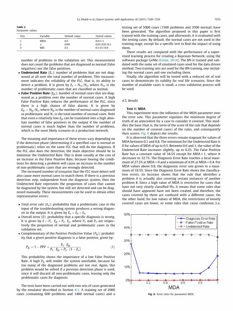
Table 2Parameter values.

Test Variable Default value Tested values

1 MDA 0.5 0:0.1:12 a 0.04 0.01:0.01:0.23 MIS 0.1 0.1:0.1:0.9

E.J. Khatib et al. / Expert Systems with Applications 42 (2015) 7549–7559 7555

number of problems in the validation set. This measurementdoes not count the problems that are diagnosed as normal (falsenegatives) nor the false positives.� Undetected Rate (Eu): number of problems that are not diag-

nosed at all over the total number of problems. This measure-ment indicates the reliability of the FLC, that is, its ability todetect a problem. It is given by Eu ¼ Nun=Np, where Nun is thenumber of problematic cases that are classified as normal.� False Positive Rate (Efp): number of normal cases that are diag-

nosed as a problem over the number of normal cases. A highFalse Positive Rate reduces the performance of the FLC, sincethere is a high chance of false alarms. It is given byEfp ¼ Nfp=Nn, where Nfp is the number of normal cases diagnosedas problematic and Nn is the total number of normal cases. Notethat even a relatively low Efp can be translated into a high abso-lute number of false positives in the output if the number ofnormal cases is much higher than the number of problems,which is the most likely scenario in a production network.

The meaning and importance of these errors vary depending onif the detection phase (determining if a specified case is normal orproblematic) relies on the same FLC that will do the diagnosis. Ifthe FLC also does the detection, the main objective should be tominimize the Undetected Rate. This is done usually at the cost ofan increase in the False Positive Rate, because loosing the condi-tions for detecting a problem will cause an increase in the numberof non-problematic cases that are wrongly detected.

The increased number of scenarios that the FLC must detect willalso cause more normal cases to match them. If there is a previousdetection step, independent from the diagnosis system, then theUndetected Rate represents the proportion of cases that cannotbe diagnosed by the system, but still are detected and can be diag-nosed manually. These measurements can be used to obtain otherrepresentative errors:

� Total error rate (Ep): probability that a problematic case in theinput of the troubleshooting system produces a wrong diagno-sis in the output. It is given by Ep ¼ Ed þ Eu.� Overall error (E): probability that a specific diagnosis is wrong.

It is given by E ¼ Pn � Efp þ Pp � Ep, where Pn and Pp are respec-tively the proportion of normal and problematic cases in thevalidation set.� Complementary of the Positive Predictive Value (Pfp): probabil-

ity that a given positive diagnosis is a false positive, given by:

Fig. 6. Error rates for parameter MDA.

Pfp ¼ 1� PPV ¼ Pn � Efp

Pn � Efp þ Pp � ð1� EuÞð1Þ

This probability shows the importance of a low False PositiveRate. A high Pfp will render the system unreliable, because fartoo many of the diagnosed problems are not real. Again, thisproblem would be solved if a previous detection phase is used,since it will discard all non-problematic cases, leaving only theproblematic cases for diagnosis.

The tests have been carried out with two sets of cases generatedby the emulator described in Section 4.1. A training set of 2000cases (containing 600 problems and 1400 normal cases) and a

testing set of 5000 cases (1500 problems and 3500 normal) havebeen generated. The algorithm proposed in this paper is firsttrained with the training cases, and afterwards, it is evaluated withthe testing cases. By default, the normal cases are not used in thetraining stage, except for a specific test to find the impact of usingthem.

These results are compared with the performance of a super-vised learning process for creating a Bayesian Network, using thesoftware package GeNIe (Genie, 2014). The BN is trained and vali-dated with the same set of emulated cases used for the data drivenmethod. Two training sets are used for the BN training, one includ-ing the normal cases and one excluding them.

Finally, the algorithm will be tested with a reduced set of realcases to demonstrate its validity for real life scenarios. Since thenumber of available cases is small, a cross validation process willbe used.

4.3. Results

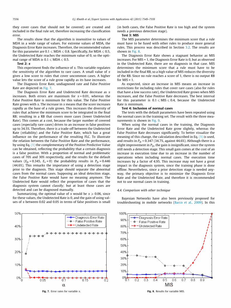
Test 1: MDAThis experiment tests the influence of the MDA parameter over

the error rate. This parameter regulates the minimum degree oftruth of an antecedent for a case to consider it covered. This mod-ifies the base (that is, the term of the score of the rule that dependson the number of covered cases) of the rules, and consequentlytheir scores. Fig. 6 depicts the results.

It is observed that the three errors remain stagnant for values ofMDA between 0.1 and 0.8. The minimum for the Undetected Rate is0 for values of MDA of up to 0.5. Between 0.6 and 1, the value of theUndetected Rate increases slightly, up to 0.2%. The False PositiveRate has a constant value of 34.5% except for MDA = 1, where itdecreases to 32.7%. The Diagnosis Error Rate reaches a local maxi-mum of 27.5% at MDA = 0 and a minimum of 4.9% at MDA = 0.4. ForMDA values above 0.8, the diagnostic error rate grows to a maxi-mum of 18.5%. Since the Diagnosis Error Rate shows the classifica-tion errors, its increase shows that the rule that identifies aproblem A is actually also covering certain instances of anotherproblem B. Since a high value of MDA is restrictive for cases thathave not very clearly classified PIs, it means that some rules thatshould have appeared have not been created, and therefore, thecases covered by them are confused with a different cause. Onthe other hand, for low values of MDA, the restrictions of looselycovered cases are lower, so some rules that cause confusion (i.e.

7556 E.J. Khatib et al. / Expert Systems with Applications 42 (2015) 7549–7559

they cover cases that should not be covered) are created andincluded in the final rule set, therefore increasing the classificationerror.

The results show that the algorithm is insensitive to values ofMDA in a wide range of values. For extreme values of MDA, theDiagnosis Error Rate increases. Therefore, the recommended valuesfor this parameter are 0.1 6MDA 6 0.8. Specifically, for MDA 6 0.5,the Undetected Rate reaches the minimum value of 0, so the opti-mal range of MDA is 0.1 6MDA 6 0.5.

Test 2: aThis experiment finds the influence of a. This variable regulates

the sensitivity of the algorithm to rare cases. A small value of agives a low score to rules that cover uncommon cases. A highervalue lets the score of a rule grow rapidly as its base increases.

The Diagnosis Error Rate, undiagnosed rate and False PositiveRate are depicted in Fig. 7.

The Diagnosis Error Rate and Undetected Rate decrease as aincreases. Both errors are maximum for a = 0.01, whereas theFalse Positive Rate is minimum for this value. The False PositiveRate grows with a. The increase in a means that the score increasesrapidly as the base of a rule grows. This increases the diversity ofrules that achieve the minimum score to be integrated in the finalRB; resulting in a RB that covers more cases (lower UndetectedRate). This comes at a cost, because the larger number of coveredcases (especially rare cases) drives to an increase in false positivesup to 34.5%. Therefore, there is a trade-off between the UndetectedRate (reliability) and the False Positive Rate, which has a greatinfluence on the performance of the resulting FLC. To illustratethe relation between the False Positive Rate and the performance,by using Eq. (1) the complementary of the Positive Predictive Valuecan be obtained, reflecting the probability that a certain diagnosisis a false positive. With a proportion of normal and problematiccases of 70% and 30% respectively, and the results for the defaultvalues (Efp = 0.345, Eu = 0) the probability results in Pfp = 0.446(44.6%). This remarks the importance of using a detection stageprior to the diagnosis. This stage should separate the abnormalcases from the normal cases. Supposing an ideal detection stage,the False Positive Rate would have no meaning anymore. TheUndetected Rate would reflect the proportion of cases that thediagnosis system cannot classify; but at least those cases aredetected and can be diagnosed manually.

Summarizing, the optimal value of a would be a P 0.06, sincefor these values, the Undetected Rate is 0, and the gain of using val-ues of a between 0.02 and 0.05 in terms of false positives is small

Fig. 7. Error rates for variable a.

(in both cases, the False Positive Rate is too high and the systemneeds a previous detection stage).

Test 3: MISThe MIS parameter determines the minimum score that a rule

must have to be fused with other rules to produce more generalrules. This process was described in Section 3.2. The results areshown in Fig. 8.

The Diagnosis Error Rate shows a stagnant behavior as MISincreases. For MIS = 1, the Diagnosis Error Rate is 0, but as observedin the Undetected Rate, there are no diagnosis in that case. MISdetermines the minimum score that a rule must have to beincluded in the final RB, so a high value of MIS reduces the diversityof the RB. Since no rule reaches a score of 1, there is no output RBfor MIS = 1.

As expected, since an increase in MIS means an increase inrestrictions for including rules that cover rare cases (also for rulesthat have a low success rate), the Undetected Rate grows when MISincreases, and the False Positive Rate decreases. The best intervalfor this parameter is 0.1 6MIS 6 0.4, because the UndetectedRate is minimum.

Test 4: Inclusion of normal casesThe tests with the default parameters have been repeated using

the normal cases in the training set. The result with the three mea-surements is shown in Fig. 9.

When using the normal cases in the training, the DiagnosisError Rate and the Undetected Rate grow slightly, whereas theFalse Positive Rate decreases significantly. To better visualize themeaning of this change, the calculation described in Eq. (1) is used,and results in Pfp = 0.347 (34.7%, against 44.6%). Although there is aslight improvement in Pfp, the gain is insignificant, since the systemstill needs a detection stage. This small gain comes at the cost of anincrease in execution time due to an increase in the number ofoperations when including normal cases. The execution timeincreases by a factor of 4.95. This increase may not have a greatimpact in the diagnosis system, since the training phase is doneoffline. Nevertheless, since a prior detection stage is needed any-way, the primary objective is to minimize the Diagnosis ErrorRate and the Undetected Rate, and therefore it is recommendednot to use normal cases in training.

4.4. Comparison with other technique

Bayesian Networks have also been previously proposed fortroubleshooting in mobile networks (Barco et al., 2009). In this

Fig. 8. Results for variable MIS.

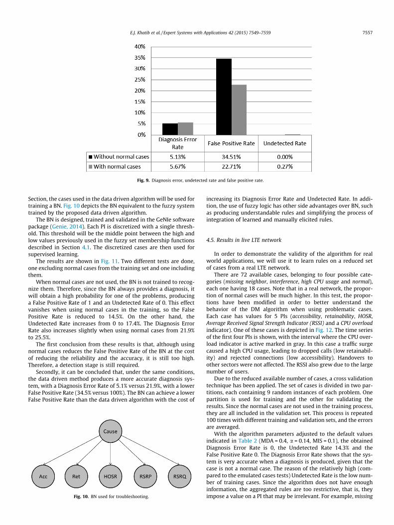
Fig. 9. Diagnosis error, undetected rate and false positive rate.

E.J. Khatib et al. / Expert Systems with Applications 42 (2015) 7549–7559 7557

Section, the cases used in the data driven algorithm will be used fortraining a BN. Fig. 10 depicts the BN equivalent to the fuzzy systemtrained by the proposed data driven algorithm.

The BN is designed, trained and validated in the GeNIe softwarepackage (Genie, 2014). Each PI is discretized with a single thresh-old. This threshold will be the middle point between the high andlow values previously used in the fuzzy set membership functionsdescribed in Section 4.1. The discretized cases are then used forsupervised learning.

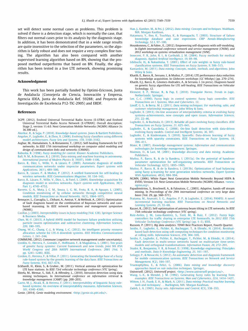
The results are shown in Fig. 11. Two different tests are done,one excluding normal cases from the training set and one includingthem.

When normal cases are not used, the BN is not trained to recog-nize them. Therefore, since the BN always provides a diagnosis, itwill obtain a high probability for one of the problems, producinga False Positive Rate of 1 and an Undetected Rate of 0. This effectvanishes when using normal cases in the training, so the FalsePositive Rate is reduced to 14.5%. On the other hand, theUndetected Rate increases from 0 to 17.4%. The Diagnosis ErrorRate also increases slightly when using normal cases from 21.9%to 25.5%.

The first conclusion from these results is that, although usingnormal cases reduces the False Positive Rate of the BN at the costof reducing the reliability and the accuracy, it is still too high.Therefore, a detection stage is still required.

Secondly, it can be concluded that, under the same conditions,the data driven method produces a more accurate diagnosis sys-tem, with a Diagnosis Error Rate of 5.1% versus 21.9%, with a lowerFalse Positive Rate (34.5% versus 100%). The BN can achieve a lowerFalse Positive Rate than the data driven algorithm with the cost of

Fig. 10. BN used for troubleshooting.

increasing its Diagnosis Error Rate and Undetected Rate. In addi-tion, the use of fuzzy logic has other side advantages over BN, suchas producing understandable rules and simplifying the process ofintegration of learned and manually elicited rules.

4.5. Results in live LTE network

In order to demonstrate the validity of the algorithm for realworld applications, we will use it to learn rules on a reduced setof cases from a real LTE network.

There are 72 available cases, belonging to four possible cate-gories (missing neighbor, interference, high CPU usage and normal),each one having 18 cases. Note that in a real network, the propor-tion of normal cases will be much higher. In this test, the propor-tions have been modified in order to better understand thebehavior of the DM algorithm when using problematic cases.Each case has values for 5 PIs (accessibility, retainability, HOSR,Average Received Signal Strength Indicator (RSSI) and a CPU overloadindicator). One of these cases is depicted in Fig. 12. The time seriesof the first four PIs is shown, with the interval where the CPU over-load indicator is active marked in gray. In this case a traffic surgecaused a high CPU usage, leading to dropped calls (low retainabil-ity) and rejected connections (low accessibility). Handovers toother sectors were not affected. The RSSI also grew due to the largenumber of users.

Due to the reduced available number of cases, a cross validationtechnique has been applied. The set of cases is divided in two par-titions, each containing 9 random instances of each problem. Onepartition is used for training and the other for validating theresults. Since the normal cases are not used in the training process,they are all included in the validation set. This process is repeated100 times with different training and validation sets, and the errorsare averaged.

With the algorithm parameters adjusted to the default valuesindicated in Table 2 (MDA = 0.4, a = 0.14, MIS = 0.1), the obtainedDiagnosis Error Rate is 0, the Undetected Rate 14.3% and theFalse Positive Rate 0. The Diagnosis Error Rate shows that the sys-tem is very accurate when a diagnosis is produced, given that thecase is not a normal case. The reason of the relatively high (com-pared to the emulated cases tests) Undetected Rate is the low num-ber of training cases. Since the algorithm does not have enoughinformation, the aggregated rules are too restrictive, that is, theyimpose a value on a PI that may be irrelevant. For example, missing

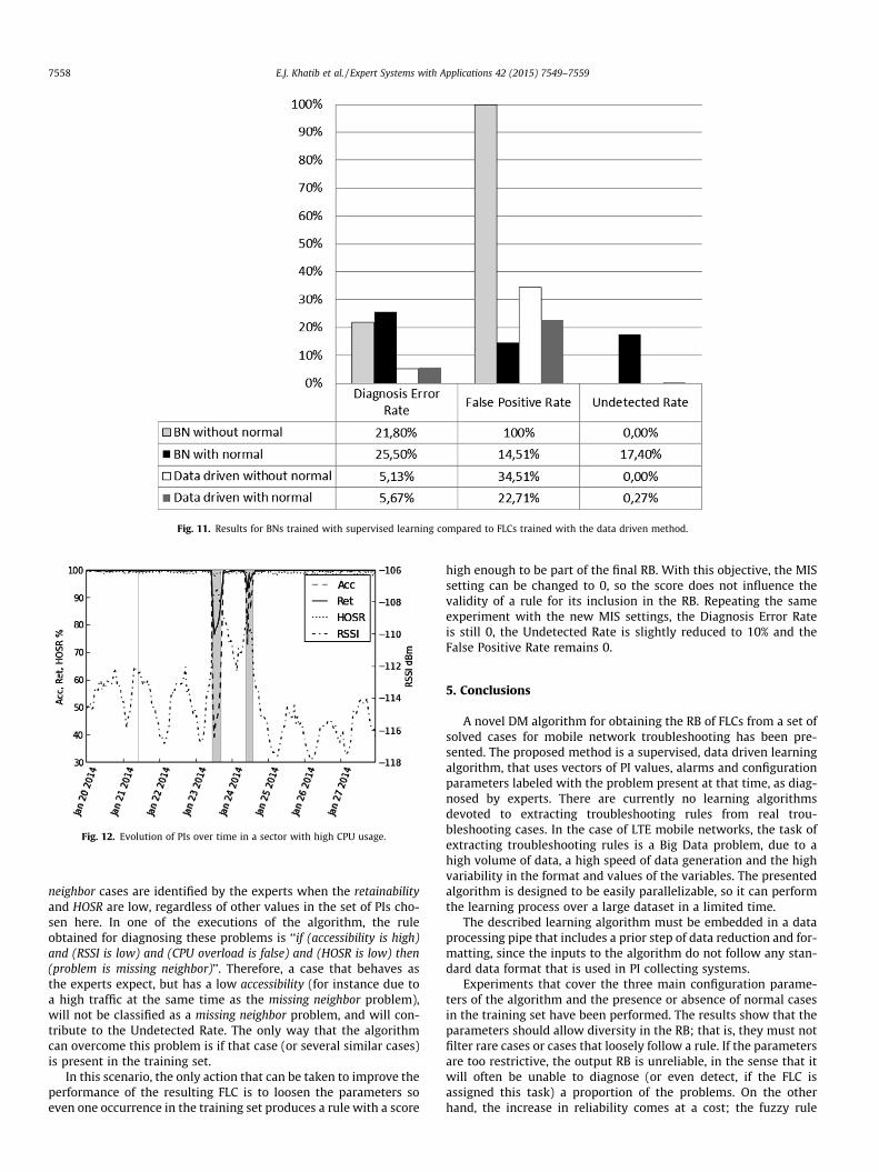
Fig. 11. Results for BNs trained with supervised learning compared to FLCs trained with the data driven method.

Fig. 12. Evolution of PIs over time in a sector with high CPU usage.

7558 E.J. Khatib et al. / Expert Systems with Applications 42 (2015) 7549–7559

neighbor cases are identified by the experts when the retainabilityand HOSR are low, regardless of other values in the set of PIs cho-sen here. In one of the executions of the algorithm, the ruleobtained for diagnosing these problems is ‘‘if (accessibility is high)and (RSSI is low) and (CPU overload is false) and (HOSR is low) then(problem is missing neighbor)’’. Therefore, a case that behaves asthe experts expect, but has a low accessibility (for instance due toa high traffic at the same time as the missing neighbor problem),will not be classified as a missing neighbor problem, and will con-tribute to the Undetected Rate. The only way that the algorithmcan overcome this problem is if that case (or several similar cases)is present in the training set.

In this scenario, the only action that can be taken to improve theperformance of the resulting FLC is to loosen the parameters soeven one occurrence in the training set produces a rule with a score

high enough to be part of the final RB. With this objective, the MISsetting can be changed to 0, so the score does not influence thevalidity of a rule for its inclusion in the RB. Repeating the sameexperiment with the new MIS settings, the Diagnosis Error Rateis still 0, the Undetected Rate is slightly reduced to 10% and theFalse Positive Rate remains 0.

5. Conclusions

A novel DM algorithm for obtaining the RB of FLCs from a set ofsolved cases for mobile network troubleshooting has been pre-sented. The proposed method is a supervised, data driven learningalgorithm, that uses vectors of PI values, alarms and configurationparameters labeled with the problem present at that time, as diag-nosed by experts. There are currently no learning algorithmsdevoted to extracting troubleshooting rules from real trou-bleshooting cases. In the case of LTE mobile networks, the task ofextracting troubleshooting rules is a Big Data problem, due to ahigh volume of data, a high speed of data generation and the highvariability in the format and values of the variables. The presentedalgorithm is designed to be easily parallelizable, so it can performthe learning process over a large dataset in a limited time.

The described learning algorithm must be embedded in a dataprocessing pipe that includes a prior step of data reduction and for-matting, since the inputs to the algorithm do not follow any stan-dard data format that is used in PI collecting systems.

Experiments that cover the three main configuration parame-ters of the algorithm and the presence or absence of normal casesin the training set have been performed. The results show that theparameters should allow diversity in the RB; that is, they must notfilter rare cases or cases that loosely follow a rule. If the parametersare too restrictive, the output RB is unreliable, in the sense that itwill often be unable to diagnose (or even detect, if the FLC isassigned this task) a proportion of the problems. On the otherhand, the increase in reliability comes at a cost; the fuzzy rule

E.J. Khatib et al. / Expert Systems with Applications 42 (2015) 7549–7559 7559

set will detect some normal cases as problems. This problem issolved if there is a detection stage, which is normally the case, thatfilters out normal cases prior to its analysis by the diagnosis stage.In addition, it has been demonstrated that in a wide range resultsare quite insensitive to the selection of the parameters, so the algo-rithm is fairly robust and does not require a very complex fine tun-ing. The algorithm has also been compared with anothersupervised learning algorithm based on BN, showing that the pro-posed method outperforms that based on BN. Finally, the algo-rithm has been tested in a live LTE network, showing promisingresults.

Acknowledgment

This work has been partially funded by Optimi-Ericsson, Juntade Andalucía (Consejería de Ciencia, Innovación y Empresa,Agencia IDEA, Junta de Andalucía Ref. 59288; and Proyecto deInvestigación de Excelencia P12-TIC-2905) and ERDF.

References

3GPP, (2012). Evolved Universal Terrestrial Radio Access (E-UTRA) and EvolvedUniversal Terrestrial Radio Access Network (E-UTRAN); Overall description;Stage 2, version 11.4.0. Next Generation Mobile Networks (NGMN) Alliance (ts36.300 ed.).

Akerkar, R., & Sajja, P. (2010). Knowledge-based systems. Jones & Bartlett Publishers.Angelov, P., Lughofer, E., & Zhou, X. (2008). Evolving fuzzy classifiers using different

model architectures. Fuzzy Sets and Systems, 159, 3160–3182.Asghar, M., Hamalainen, S., & Ristaniemi, T., (2012). Self-healing framework for LTE

networks. In IEEE 17th international workshop on computer aided modeling anddesign of communication links and networks (CAMAD).

Babuska, R. (1998). Fuzzy modeling for control. Kluwer Academic Publishers.Ball, N. M., & Brunner, R. J. (2010). Data mining and machine learning in astronomy.

International Journal of Modern Physics D, 19(07), 1049–1106.Barco, R., Díez, L., Wille, V., & Lázaro, P. (2009). Automatic diagnosis of mobile

communication networks under imprecise parameters. Expert systems withApplications, 36(1), 489–500.

Barco, R., Lázaro, P., & Muñoz, P. (2012). A unified framework for self-healing inwireless networks. IEEE Communications Magazine, 50, 134–142.

Barco, R., Lázaro, P., Wille, V., Díez, L., & Patel, S. (2009). Knowledge acquisition fordiagnosis model in wireless networks. Expert systems with Applications, 36(3,Part 1), 4745–4752.

Barreto, G. A., Mota, J. C. M., Souza, L. G. M., Frota, R. A., & Aguayo, L. (2005).Condition monitoring of 3g cellular networks through competitive neuralmodels. IEEE Transactions on Neural Networks, 16(5), 1064–1075.

Bennacer, L., Ciavaglia, L., Chibani, A., Amirat, Y., & Mellouk, A., (2012). Optimizationof fault diagnosis based on the combination of Bayesian networks and case-based reasoning. In IEEE network operations and management symposium(NOMS).

Casillas, J. (2003). Interpretability issues in fuzzy modeling (Vol. 128). Springer Science& Business Media.

Chen, M.-Y. (2013). A hybrid ANFIS model for business failure prediction utilizingparticle swarm optimization and subtractive clustering. Information Sciences,220, 180–195.

Chung, W.-C., Chang, C.-J., & Wang, L.-C. (2012). An intelligent priority resourceallocation scheme for LTE-A downlink systems. IEEE Wireless CommunicationsLetters, 1, 241–244.

COMMUNE, (2012). Commune (cognitive network management under uncertainty).Cordón, O., Herrera, F., Gomide, F., Hoffmann, F., & Magdalena, L. (2001). Ten years

of genetic fuzzy systems: Current framework and new trends. Joint 9th IFSAWorld Congress and 20th NAFIPS International Conference, 2001 (Vol. 3,pp. 1241–1246). IEEE.

Cordon, O., Herrera, F., & Villar, P. (2011). Generating the knowledge base of a fuzzyrule-based system by the genetic learning of the data base. IEEE Transactions onFuzzy Systems, 9(4), 667–674.

Eckhardt, H., Klein, S., & Gruber., M. (2011). Vertical antenna tilt optimization forLTE base stations. In IEEE 73rd vehicular technology conference (VTC Spring).

Ektefa, M., Memar, S., Sidi, F., & Affendey, L., (2010). Intrusion detection using datamining techniques. In International conference on information retrieval &knowledge management (CAMP) (pp. 200–203).

Gacto, M. J., Alcalá, R., & Herrera, F. (2011). Interpretability of linguistic fuzzy rule-based systems: An overview of interpretability measures. Information Sciences,181, 4340–4360.

Genie. (2014). Genie modeling environment. <http://genie.sis.pitt.edu/>.

Han, J., Kamber, M., & Pei, J. (2012). Data mining: Concepts and techniques. Waltham,MA: Morgan Kaufman.

Hatamura, Y., Ilno, K., Tsuchlya, K., & Hamaguchi, T. (2003). Structure of failureknowledge database and case expression. CIRP Annals-ManufacturingTechnology, 52.1, 97–100.

Hounkonnou, C., & Fabre., E., (2012). Empowering self-diagnosis with self-modeling.In Eighth international conference network and service management (CNSM), and2012 workshop on systems virtualization management (SVM).

Innocent, P. R., John, R. I., & Garibaldi, J. M. (2004). Fuzzy methods for medicaldiagnosis. Applied Artificial Intelligence, 19, 69–98.

Ishibuchi, H., & Nakashima, T. (2001). Effect of rule weights in fuzzy rule-basedclassification systems. IEEE Transactions on Fuzzy Systems, 9, 506–515.

Kantardzic, M. (2011). Data mining: Concepts, models, methods, and algorithms. JohnWiley & Sons.

Khatib, E., Barco, R., Serrano, I., & Muñoz, P., (2014). LTE performance data reductionfor knowledge acquisition. In Globecom workshops (GC Wkshps) (pp. 270–274).

Khatib, E.J., Barco, R., Góomez-Andrades, A., & Serrano, I. (in press). Diagnosis basedon genetic fuzzy algorithms for LTE self-healing. IEEE Transactions on VehicularTechnology, 12.

Klement, E. P., Mesiar, R., & Pap, E. (2010). Triangular Norms. Trends in Logic.Netherlands: Springer.

Lee, C.-C. (1990). Fuzzy logic in control systems: fuzzy logic controller. IEEETransactions on I. Systems, Man and Cybernetics, 12.

Linoff, G. S., & Berry, M. J. (2011). Data mining techniques: For marketing, sales, andcustomer relationship management. John Wiley & Sons.

Lughofer, E. (2013). On-line assurance of interpretability criteria in evolving fuzzysystems–achievements, new concepts and open issues. Information Sciences,251, 22–46.

Lughofer, E., & Buchtala, O. (2013). Reliable all-pairs evolving fuzzy classifiers. IEEETransactions on Fuzzy Systems, 21, 625–641.

Lughofer, E., & Guardiola, C. (2008). On-line fault detection with data-drivenevolving fuzzy models. Control and Intelligent Systems, 36, 307.

Lughofer, E., & Kindermann, S. (2010). Sparsefis: Data-driven learning of fuzzysystems with sparsity constraints. IEEE Transactions on Fuzzy Systems, 18,396–411.

Maier, R. (2007). Knowledge management systems: Information and communicationtechnologies for knowledge management. Springer.

Maimon, O., & Last, M. (2001). Knowledge discovery and data mining. AcademicPublishers.

Muñoz, P., Barco, R., & de la Bandera, I. (2013a). On the potential of handoverparameter optimization for self-organizing networks. IEEE Transactions onVehicular Technology, 62(5), 1895–1905.

Muñoz, P., Barco, R., & de la Bandera, I. (2013b). Optimization of load balancingusing fuzzy q-learning for next generation wireless networks. Expert SystemsWith Applications, 40(4), 984–994.

NGMN, (2006). White Paper Next Generation Mobile Networks Beyond HSPA &EVDO, Version 3.0. Next Generation Mobile Networks (NGMN) Alliance. <www.ngmn.org>.

Papadimitriou, S., Brockwell, A., & Faloutsos, C., (2003). Adaptive, hands-off streammining. In Proceedings of the 29th international conference on very large databases (Vol. 29, pp. 560–571).

Pratama, M., Anavatti, S. G., Angelov, P. P., & Lughofer, E. (2014). PANFIS: A novelincremental learning machine. IEEE Transactions on Neural Networks andLearning Systems, 25, 55–68.

Razavi, R., (2012). Self-optimisation of antenna beam tilting in LTE networks. In IEEE75th vehicular technology conference (VTC spring).

Ruiz-Aviles, J. M., Luna-Ramírez, S., Toril, M., & Ruiz, F. (2012). Fuzzy logiccontrollers for traffic sharing in enterprise LTE femtocells. In 2012 IEEE 75thVehicular Technology Conference (VTC Spring) (pp. 1–5). IEEE.

Russom, P. (2011). Big data analytics. TDWI Best Practices Report, Fourth Quarter.Serdio, F., Lughofer, E., Pichler, K., Buchegger, T., & Efendic, H. (2014). Residual-

based fault detection using soft computing techniques for condition monitoringat rolling mills. Information Sciences, 259, 304–320.

Serdio, F., Lughofer, E., Pichler, K., Buchegger, T., Pichler, M., & Efendic, H. (2014).Fault detection in multi-sensor networks based on multivariate time-seriesmodels and orthogonal transformations. Information Fusion, 20, 272–291.

Studer, R., Benjamins, V. R., & Fensel, D. (1998). Knowledge engineering: Principlesand methods. Data & Knowledge Engineering, 25, 161–197.

Szilagyi, P., & Novaczki, S. (2012). An automatic detection and diagnosis frameworkfor mobile communication systems. IEEE Transactions on Network and ServiceManagement, 9(2), 184–197.

Triantaphyllou, E., & Felici, G. (2006). Data mining and knowledge discoveryapproaches based on rule induction techniques. Springer.

Univerself. (2012). Univerself project. <http://www.univerself-project.eu/>.Wang, L.-X., & Mendel, J. M. (1992). Generating fuzzy rules by learning from

examples. IEEE Transactions on Systems, Man and Cybernetics, 22.6, 1414–1427.Witten, I. H., Frank, E. H., & Mark, A. (2011). Data mining: Practical machine learning

tools and techniques/. . .. Burlington, MA: Morgan Kaufman.Zadeh, L. A. (1965). Fuzzy sets. Information and Control, 8(3), 338–353.