explaining credit default swap spreads with the … credit default swap spreads with the equity...
TRANSCRIPT

Finance and Economics Discussion Series Divisions of Research & Statistics and Monetary Affairs
Federal Reserve Board, Washington, D.C.
Explaining Credit Default Swap Spreads with the Equity Volatility and Jump Risks of Individual Firms
Benjamin Yibin Zhang, Hao Zhou, and Haibin Zhu 2005-63
NOTE: Staff working papers in the Finance and Economics Discussion Series (FEDS) are preliminary materials circulated to stimulate discussion and critical comment. The analysis and conclusions set forth are those of the authors and do not indicate concurrence by other members of the research staff or the Board of Governors. References in publications to the Finance and Economics Discussion Series (other than acknowledgement) should be cleared with the author(s) to protect the tentative character of these papers.
Explaining Credit Default Swap Spreads with the
Equity Volatility and Jump Risks of Individual Firms∗
Benjamin Yibin Zhang†
Hao Zhou‡
Haibin Zhu§
First Draft: December 2004This Version: December 2005
Abstract
A structural model with stochastic volatility and jumps implies specific relationshipsbetween observed equity returns and credit spreads. This paper explores such effects inthe credit default swap (CDS) market. We use a novel approach to identify the realizedjumps of individual equities from high frequency data. Our empirical results suggestthat volatility risk alone predicts 50 percent of the variation in CDS spreads, while jumprisk alone forecasts 19 percent. After controlling for credit ratings, macroeconomicconditions, and firms’ balance sheet information, we can explain 77 percent of thetotal variation. Moreover, the pricing effects of volatility and jump measures varyconsistently across investment-grade and high-yield entities. The estimated nonlineareffects of volatility and jumps are in line with the model-implied relationships betweenequity returns and credit spreads.
JEL Classification Numbers: G12, G13, C14.Keywords: Structural Model; Stochastic Volatility; Jumps; Credit Spread; CreditDefault Swap; Nonlinear Effect; High-Frequency Data.
∗The views presented here are solely those of the authors and do not necessarily represent those of FitchRatings, the Federal Reserve Board, or the Bank for International Settlements. We thank Jeffrey Amato,Ren-Raw Chen, Greg Duffee, Mike Gibson, Jean Helwege, Jingzhi Huang, and George Tauchen for detaileddiscussions. Comments from seminar participants at the Federal Reserve Board, the 2005 FDIC DerivativeConference, the Bank for International Settlements, the 2005 Pacific Basin Conference at Rutgers, and the2005 C.R.E.D.I.T Conference in Venice are greatly appreciated. We also thank Christopher Karlsten forediting advice.
†Benjamin Yibin Zhang, Fitch Ratings, One State Street Plaza, New York, NY 10004, USA. Tel.: 1-212-908-0201. Fax: 1-914-613-0948. E-mail: [email protected].
‡Hao Zhou, Federal Reserve Board, Mail Stop 91, Washington, DC 20551, USA. Tel.: 1-202-452-3360.Fax: 1-202-728-5887. E-mail: [email protected].
§Haibin Zhu, Bank for International Settlements, Centralbahnplatz 2, 4002 Basel, Switzerland. Tel.:41-61-280-9164. Fax: 41-61-280-9100. E-mail: [email protected].

Explaining Credit Default Swap Spreads with the
Equity Volatility and Jump Risks of Individual Firms
Abstract
A structural model with stochastic volatility and jumps implies specific relationships
between observed equity returns and credit spreads. This paper explores such effects in the
credit default swap (CDS) market. We use a novel approach to identify the realized jumps
of individual equities from high frequency data. Our empirical results suggest that volatility
risk alone predicts 50 percent of the variation in CDS spreads, while jump risk alone forecasts
19 percent. After controlling for credit ratings, macroeconomic conditions, and firms’ balance
sheet information, we can explain 77 percent of the total variation. Moreover, the pricing
effects of volatility and jump measures vary consistently across investment-grade and high-
yield entities. The estimated nonlinear effects of volatility and jumps are in line with the
model-implied relationships between equity returns and credit spreads.
JEL Classification Numbers: G12, G13, C14.
Keywords: Structural Model; Stochastic Volatility; Jumps; Credit Spread; Credit Default
Swap; Nonlinear Effect; High-Frequency Data.

1 Introduction
The empirical tests of structural models of credit risk indicate that such models have been
unsuccessful. Methods of strict estimation or calibration provide evidence that the models are
deficient: Predicted credit spreads are far below observed ones (Jones, Mason, and Rosenfeld,
1984), the structural variables explain little of the credit spread variation (Huang and Huang,
2003), and pricing error is large for corporate bonds (Eom, Helwege, and Huang, 2004). More
flexible regression analysis, although confirming the validity of the cross-sectional or long-run
factors in predicting the bond spread, suggests that the power of default risk factors to explain
the credit spread is still small (Collin-Dufresne, Goldstein, and Martin, 2001). Regression
analysis also indicates that the temporal changes in the bond spread are not directly related
to expected default loss (Elton, Gruber, Agrawal, and Mann, 2001) and that the forecasting
power of long-run volatility cannot be reconciled with the classical Merton model (1974)
(Campbell and Taksler, 2003). These negative findings are robust to the extensions of
stochastic interest rates (Longstaff and Schwartz, 1995), endogenously determined default
boundaries (Leland, 1994; Leland and Toft, 1996), strategic defaults (Anderson, Sundaresan,
and Tychon, 1996; Mella-Barral and Perraudin, 1997), and mean-reverting leverage ratios
(Collin-Dufresne and Goldstein, 2001).
To address these negative findings, we propose a novel approach for explaining credit
spread variation. We argue that incorporating stochastic volatility and jumps into the asset-
value process (Huang, 2005) may enable structural variables to adequately explain credit
spread variations, especially in the time-series dimension. The most important finding in
Campbell and Taksler (2003) is that the recent increases in corporate yields can be explained
by the upward trend in idiosyncratic equity volatility, but the magnitude of the volatility
coefficient is clearly inconsistent with the structural model of constant volatility (Merton,
1974). Nevertheless, in theory incorporating jumps, should lead to a better explanation of
the level of credit spreads for investment-grade bonds at short maturities (Zhou, 2001), but
the empirical evidence is rather mixed. Collin-Dufresne, Goldstein, and Martin (2001) and
Collin-Dufresne, Goldstein, and Helwege (2003) use a market-based jump-risk measure and
find that it explains only a very small proportion of the credit spread. Cremers, Driessen,
Maenhout, and Weinbaum (2004a,b) instead rely on individual option-implied skewness and
find some positive evidence. We demonstrate numerically that adding stochastic volatility
and jumps to the classical Merton model (1974) can dramatically increase the flexibility
of the entire credit curve, potentially enabling the model to better match observed yield
spreads and to better forecast temporal variation. In particular, we outline the testable
1

empirical hypotheses concerning the relationships between the observable equity returns
and observable credit spreads implied by the underlying asset-return process. This step
is important, as asset value and volatility are generally not observable and the testing of
structural models must rely heavily on the observable equity return and observable default
spread.
Our methodology builds on the recent literature on measuring volatility and jumps from
high-frequency data. We adopt both historical and realized measures as proxies for the
temporal variation in equity returns, and we adopt realized jump measures as proxies for
various aspects of jump risk. Our main innovation is to use the high-frequency equity re-
turns of individual firms to detect the realized jumps on each day. Recent literature suggests
that realized variance measures from high-frequency data provide a more accurate measure
of short-term volatility than from low-frequency data (Andersen, Bollerslev, Diebold, and
Labys, 2001; Barndorff-Nielsen and Shephard, 2002; Meddahi, 2002). Furthermore, the con-
tributions of the continuous and jump components of realized variance can be separated
by analyzing the difference between bipower variation and quadratic variation (Barndorff-
Nielsen and Shephard, 2004; Andersen, Bollerslev, and Diebold, 2005; Huang and Tauchen,
2005). Considering that jumps on financial markets are usually rare and large, we further
assume that (1) there is at most one jump per day and (2) jump size dominates daily return
when it occurs. These assumptions help us to identify the daily realized jumps of equity
returns, as in Tauchen and Zhou (2005). From these realized jumps, we can estimate the
jump intensity, jump mean, and jump volatility, and we can directly test the connections
between equity returns and credit spreads implied by a stylized structural model that has
incorporated stochastic volatility and jumps into the asset-value process.
The empirical success of our approach also depends on a direct measure of credit default
spreads. For this measure, we rely on the credit default swap (CDS) premium, the most
popular instrument in the rapidly growing credit derivatives market. Compared with corpo-
rate bond spreads, which were widely used in previous studies in tests of structural models,
CDS spreads have two important advantages. First, CDS spreads provide relatively pure
pricing of the default risk of the underlying entity. The contracts are typically traded on
standardized terms. In contrast, bond spreads are more likely to be affected by differences in
contractual arrangements, such as differences related to seniority, coupon rates, embedded
options, and guarantees. For example, Longstaff, Mithal, and Neis (2005) find that a large
proportion of bond spreads are determined by liquidity factors, which do not necessarily
reflect the default risk of the underlying asset. Second, Blanco, Brennan, and March (2005)
and Zhu (2004) show that, although CDS spreads and bond spreads are quite in line with
2

each other in the long run, in the short run CDS spreads tend to respond more quickly to
changes in credit conditions. Part of the reason for the quicker response of CDS spreads may
be that they are unfunded and do not face short-sale restrictions. The fact that CDS leads
the bond market in price discovery is integral to our improved explanation of the temporal
changes in credit spread by default-risk factors.
There is a subtle difference between our empirical regression approach and the ones used
in previous studies. In contrast to the common empirical strategy that simultaneously re-
gresses credit spreads on structural variables constructed from equity or option data, we use
only the lagged explanatory variables. Under a typical structural framework, only asset re-
turn and asset volatility are exogenous processes, whereas equity return and equity volatility
as well as credit spread are all endogenously determined. Simultaneous regressions without
structural restrictions would artificially inflate the R2 values and t-statistics.
Our empirical findings suggest that long-run historical volatility, short-run realized volatil-
ity, and various jump-risk measures all have statistically significant and economically mean-
ingful effects on credit spreads. Realized jump measures explain 19 percent of total varia-
tions in credit spreads, whereas measures of the historical skewness and historical kurtosis
of jump risk explain only 3 percent. Notably, volatility and jump risks alone can predict 54
percent of the spread variations. After controlling for credit ratings, macro-financial vari-
ables, and firms’ accounting information, we find that the signs and significance of the jump
and volatility effects remain solid, and the R2 increases to 77 percent. These results are
robust to whether the fixed effect or the random effect is taken into account, an indication
that the temporal variation of default-risk factors does explain CDS spreads. More impor-
tant, the sensitivity of credit spreads to volatility and jump risk is greatly elevated from
investment-grade to high-yield entities, a finding that has implications for managing the
more risky credit portfolios. Last but not least, both the volatility-risk and the jump-risk
measures show strong nonlinear effects; this result is consistent with the hypotheses implied
by the structural model that has incorporated stochastic volatility and jumps.
The remainder of the paper is organized into four sections. Section 2 introduces the
structural link between equity and credit and discusses the methodology for disentangling
volatility and jumps through the use of high-frequency data. Section 3 then gives a brief
description of the CDS data and the structural explanatory variables. Section 4 presents the
main empirical findings regarding the role of jump and volatility risks in explaining credit
spreads. Section 5 summarizes the findings and proposes avenues of future research.
3

2 Structural motivation and econometric technique
Testing structural models of credit risk is difficult because the underlying asset value and
its volatility processes are not observable; therefore, approximations from observed equity
prices and volatilities have been a common practice. However, because the equity shares and
credit derivatives of many listed firms are traded in relatively liquid markets, researchers are
prompted to directly model the observable equity dynamics to explain and predict the credit
spreads (see, Madan and Unal, 2000; Das and Sundaram, 2004; Carr and Wu, 2005, among
others). Nevertheless, structural models can still provide important economic intuitions to
interpret the empirical linkage between equity and credit. Here we motivate our empirical
exercise by using an affine structural model to examine the model-implied equity-credit
relationship.
2.1 A stylized model with stochastic volatility and jumps
Assuming the same market environment as in Merton (1974), one can introduce stochastic
volatility (Heston, 1993) and jumps (Zhou, 2001) into the underlying firm-value process:
dAt
At
= (µ − δ − λµJ)dt +√
VtdW1t + Jtdqt, (1)
dVt = κ(θ − Vt)dt + σ√
VtdW2t, (2)
where At is the firm value, µ is the instantaneous asset return, and δ is the dividend payout
ratio. Asset jump has a Poisson mixing Gaussian distribution with dqt ∼ Poisson (λdt)
and log(1 + Jt) ∼ Normal (log(1 + µJ) − 12σ2
J , σ2J). The asset return volatility Vt follows
a square root process with long-run mean θ, mean reversion κ, and variance parameter σ.
Finally, the correlation between asset return and return volatility is corr (dW1t, dW2t) = ρ.
This specification has been extensively studied in the equity-option pricing literature (see
Bates, 1996; Bakshi et al., 1997, for example). To be suitable for pricing corporate debt, the
required assumptions are that default occurs only at maturity with a fixed default boundary
and that when default occurs, there is no bankruptcy cost and the absolute priority rule
prevails (Huang, 2005).
Using the no-arbitrage solution method of Duffie, Pan, and Singleton (2000), one can solve
the equity price St as a European call option on debt Dt with face value B and maturity
time T :
St = AtF∗
1 − Be−r(T−t)F ∗
2 , (3)
4
where F ∗
1 and F ∗
2 are so-called risk-neutral probabilities.1 Therefore, the debt value can be
expressed as Dt = At − St, and its price is Pt = Dt/B. The credit default spread is then
given by
Rt − r = − 1
T − tlog(Pt) − r, (6)
where Rt is the risky interest rate and r is the risk-free interest rate.
2.2 The sensitivity of credit spread to asset volatility and jumps
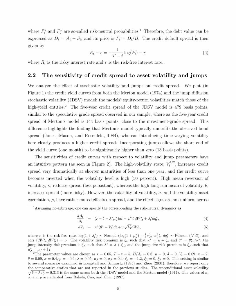
We analyze the effect of stochastic volatility and jumps on credit spread. We plot (in
Figure 1) the credit yield curves from both the Merton model (1974) and the jump diffusion
stochastic volatility (JDSV) model; the models’ equity-return volatilities match those of the
high-yield entities.2 The five-year credit spread of the JDSV model is 479 basis points,
similar to the speculative grade spread observed in our sample, where as the five-year credit
spread of Merton’s model is 144 basis points, close to the investment-grade spread. This
difference highlights the finding that Merton’s model typically underfits the observed bond
spread (Jones, Mason, and Rosenfeld, 1984), whereas introducing time-varying volatility
here clearly produces a higher credit spread. Incorporating jumps allows the short end of
the yield curve (one month) to be significantly higher than zero (13 basis points).
The sensitivities of credit curves with respect to volatility and jump parameters have
an intuitive pattern (as seen in Figure 2). The high-volatility state, V1/2t , increases credit
spread very dramatically at shorter maturities of less than one year, and the credit curve
becomes inverted when the volatility level is high (50 percent). High mean reversion of
volatility, κ, reduces spread (less persistent), whereas the high long-run mean of volatility, θ,
increases spread (more risky). However, the volatility-of-volatility, σ, and the volatility-asset
correlation, ρ, have rather muted effects on spread, and the effect signs are not uniform across
1Assuming no-arbitrage, one can specify the corresponding the risk-neutral dynamics as
dAt
At
= (r − δ − λ∗µ∗J)dt +
√
VtdW ∗1t + J∗
t dq∗t , (4)
dVt = κ∗(θ∗ − Vt)dt + σ√
VtdW ∗2t, (5)
where r is the risk-free rate, log(1 + J∗t ) ∼ Normal (log(1 + µ∗
J) − 1
2σ2
J, σ2
J), dq∗t ∼ Poisson (λ∗dt), and
corr (dW ∗1t, dW ∗
2t) = ρ. The volatility risk premium is ξv such that κ∗ = κ + ξv and θ∗ = θξv/κ∗, thejump-intensity risk premium is ξλ such that λ∗ = λ + ξλ, and the jump-size risk premium is ξJ such thatµ∗
J= µJ + ξJ .2The parameter values are chosen as r = 0.05, T − t = 5, B/At = 0.6, µ = 0, δ = 0; Vt = 0.09, κ = 2,
θ = 0.09, σ = 0.4, ρ = −0.6; λ = 0.05, µJ = 0, σJ = 0.4; ξv = −1.2, ξλ = 0, ξJ = 0. This setting is similarto several scenarios examined in Longstaff and Schwartz (1995) and Zhou (2001); therefore, we report onlythe comparative statics that are not reported in the previous studies. The unconditional asset volatility√
θ + λσ2
J= 0.313 is the same across both the JDSV model and the Merton model (1974). The values of κ,
σ, and ρ are adapted from Bakshi, Cao, and Chen (1997).
5

all maturities. Finally, the jump mean, µJ , seems to have nonmonotonic and asymmetric
effects on credit spread – that is, both positive and negative jump means will elevate the
credit spread, but negative jump means seem to raise the spread higher.3
2.3 Testable hypotheses relating equity to credit
The stochastic volatility jump diffusion model (equations 1-6) of asset-value and volatility
processes implies the following specification of equity price by applying the Ito Lemma:
dSt
St
=1
St
µt(·)dt +At
St
∂St
∂At
√
VtdW1t +1
St
∂St
∂Vt
σ√
VtdW2t
+1
St
[St(At(1 + Jt), Vt; Ω) − St(At, Vt; Ω)]dqt, (7)
where µt(·) is the instantaneous equity return, Ω is the parameter vector, At and Vt are the
latent asset and volatility processes, and St ≡ St(At, Vt; Ω). Therefore, the instantaneous
volatility Σst and jump size Js
t of the log equity price are, respectively,
Σst =
√
(
At
St
)2 (
∂St
∂At
)2
Vt +
(
σ
St
)2 (
∂St
∂Vt
)2
Vt +At
S2t
∂St
∂At
∂St
∂Vt
ρσVt, (8)
Jst = log[St(At(1 + Jt), Vt; Ω)] − log[St(At, Vt; Ω)], (9)
where Jst has unconditional mean µs
J and standard deviation σsJ , which are unknown in
closed form because of the nonlinear functional form of St(At, Vt; Ω). Obviously, the equity
volatility is driven by the two time-varying factors At and Vt, whereas the asset volatility is
simply driven by Vt. However, if asset volatility is constant (V ), then equation (8) reduces to
the standard Merton formula (1974), Σst =
√V ∂St
∂At
At
St
. Because the Poisson driving process is
the same for equity jump as it is for asset jump, it has the same intensity function: λs = λ.
The most important empirical implication is how credit spread responds to changes in
equity jump and equity volatility parameters, implied by the underlying changes in asset jump
and asset volatility parameters (Figure 3). The left column suggests that five-year credit
spread would increase linearly with the levels of asset volatility (V1/2t ) and jump intensity
(λ). Asset jump volatility (σJ) would also raise credit spread but in a nonlinear, convex
fashion. Interestingly, the asset jump mean (µJ) increases credit spread when moving away
from zero. More interestingly, the effect is nonlinear and asymmetric—the negative jump
3Since the risk premium parameters ξv, ξλ, and ξJ enter the pricing equation additively with κ, λ, andµJ , their effects on credit spreads are the same as the effects of those parameters and are hence omitted. Inaddition, the positive effects of jump intensity, λ, and jump volatility, σJ , on credit spread are similar to theeffects reported in Zhou (2001) and are hence omitted.
6

mean increases spread much more than does the positive jump mean. The reason is that
the first-order effect of jump mean changes may be offset by the drift compensator, and the
second-order effect is equivalent to jump volatility increases because of the lognormal jump
distribution.
Given the same changes in structural asset volatility and asset jump parameters, the
right column in Figure 3 plots credit spread changes as related to the equity volatility and
equity jump parameters. Clearly, equity volatility (Σst) still increases credit spread, but in
a nonlinear, convex pattern. Note that equity volatility is about three times as large as
asset volatility, mostly because of the leverage effect. Equity jump intensity (λs) is the same
as asset jump intensity, so the linear effect on credit spread is also the same. Equity jump
volatility (σsJ) has a similar positive nonlinear effect on credit spread, but the range of equity
jump volatility is nearly twice as large as that of asset jump volatility. Equity jump mean
(µsJ) also has a nonlinear, asymmetric effect on credit spread, but the equity jump mean
is more negative than the asset jump mean.4 Of course, in a linear regression setting, one
would find only the approximate negative relationship between equity jump mean and credit
spread. These relationships, illustrated in Figure 3, are qualitatively robust to alternative
settings of the structural parameters.
To summarize, the following empirical hypotheses may be tested regarding the relation-
ship between equity price and credit spread:
• H1 Equity volatility increases credit spread nonlinearly through two factors
• H2 Equity jump intensity increases credit spread linearly
• H3 Equity jump volatility increases credit spread nonlinearly
• H4 Equity jump mean affects credit spread in a nonlinear, asymmetric way; negative
jumps tend to have larger effects.
2.4 Disentangling the jump and volatility risks of equities
In this paper, we rely on the economic intuition that jumps on financial markets are rare
and large, to explicitly estimate the jump intensity, jump variance, and jump mean and to
directly assess the empirical effects of volatility and jump risks on credit spreads.
4Equity jump mean, µs
J, and standard deviation, σs
J, do not have closed-form solutions. So at each grid
of the structural parameter values µJ and σJ , we simulate asset jump 2000 times and use equation (9) tonumerically evaluate µs
Jand σs
J.
7

Let st ≡ log St denote the time t logarithmic price of the stock, which evolves in contin-
uous time as a jump diffusion process:
dst = µstdt + σs
t dWt + Jst dqt, (10)
where µst , σs
t , and Jst are, respectively, the drift, diffusion, and jump functions that may be
more general than the model-implied equity process (7). Wt is a standard Brownian motion
(or a vector of Brownian motions), dqt is a Poisson driving process with intensity λs = λ,
and Jst refers to the size of the corresponding log equity jump, which is assumed to have
mean µsJ and standard deviation σs
J . Time is measured in daily units, and the daily return rt
is defined as rst ≡ st − st−1. We have designated historical volatility, defined as the standard
deviation of daily returns, as one proxy for the volatility risk of the underlying asset-value
process (see, for example, Campbell and Taksler, 2003). The intraday returns are defined as
follows:
rst,i ≡ st,i·∆ − st,(i−1)·∆, (11)
where rst,i refers to the ith within-day return on day t and ∆ is the sampling frequency.5
Barndorff-Nielsen and Shephard (2003a,b, 2004) propose two general measures of the
quadratic variation process, realized variance and realized bipower variation, which converge
uniformly (as ∆ → 0) to different quantities of the jump diffusion process:
RVt ≡1/∆∑
i=1
(rst,i)
2 →∫ t
t−1
σ2sds +
1/∆∑
i=1
(Jst,i)
2, (12)
BVt ≡ π
2
1/∆∑
i=2
|rst,i| · |rs
t,i−1| →∫ t
t−1
σ2sds. (13)
Therefore, the asymptotic difference between realized variance and bipower variation is zero
when there is no jump and strictly positive when there is a jump. A variety of jump detec-
tion techniques have been proposed and studied by Barndorff-Nielsen and Shephard (2004),
Andersen, Bollerslev, and Diebold (2005), and Huang and Tauchen (2005). Here we adopt
the ratio test statistics, defined as follows:
RJt ≡RVt − BVt
RVt
. (14)
5That is, 1/∆ observations occurs on every trading day. Typically, the five-minute frequency is usedbecause more frequent observations may be subject to distortion from market microstructure noise (Aıt-Sahalia, Mykland, and Zhang, 2005; Bandi and Russell, 2005).
8

When appropriately scaled by its asymptotic variance, z = RJtq
Avar(RJt)converges to a
standard normal distribution.6 This test tells us whether a jump occurred during a particular
day and how much jump contributes to the total realized variance – that is, the ratio of∑1/∆
i=1 (Jst,i)
2 over RVt.
To identify the actual jump sizes, we further assume that (1) there is at most one jump
per day and (2) jump size dominates return on jump days. Following the idea of “signifi-
cant jumps” in Andersen, Bollerslev, and Diebold (2005), we use the signed square root of
significant jump variance to filter out the daily realized jumps:
Jst = sign(rs
t ) ×√
RVt − BVt × I(z > Φ−1α ), (15)
where Φ is the probability of a standard normal distribution and α is the level of significance
chosen as 0.999. The filtered realized jumps enable us to estimate the jump distribution
parameters directly:
λs =Number of jump days
Number of trading days, (16)
µsJ = Mean of Js
t , (17)
σsJ = Standard deviation of Js
t . (18)
Tauchen and Zhou (2005) show that under empirically realistic settings, this method of
identifying realized jumps and estimating jump parameters yields reliable results in finite
samples as the sample size increases and as the sampling interval shrinks. We can also
estimate the time-varying jump parameters for a rolling window, for example, λst , µs
J,t, and
σsJ,t over a one-year horizon. Equipped with this econometric technique, we are ready to
re-examine the effect of jumps on credit spreads.
3 Data
Throughout this paper, we choose to use the credit default swap (CDS) premium as a direct
measure of credit spreads. The CDS is the most popular instrument in the rapidly growing
credit derivatives market. Under a CDS contract, the protection seller promises to buy
the reference bond at its par value when a pre-defined default event occurs. In return,
the protection buyer makes periodic payments to the seller until the maturity date of the
6See Appendix A for implementation details. As in Huang and Tauchen (2005), we find that using the testlevel of 0.999 produces the most consistent results. In constructing the test statistics, we also use staggeredreturns to control for the potential problem of measurement error.
9

contract or until a credit event occurs. This periodic payment, which is usually expressed as
a percentage (in basis points) of its notional value, is called the CDS spread. By definition,
credit spread provides a pure measure of the default risk of the reference entity.7
Our CDS data are provided by Markit, a comprehensive data source that assembles a
network of industry-leading partners who contribute information across several thousand
credits on a daily basis. Using the contributed quotes, Markit creates the daily composite
quote for each CDS contract.8 Together with the pricing information, the data set also
reports average recovery rates used by data contributors in pricing each CDS contract.
In this paper, we include all CDS quotes written on U.S. entities (excluding sovereign
entities) and denominated in U.S. dollars. We eliminate the subordinated class of contracts
because of their small relevance in the database and their unappealing implications for credit
risk pricing. We focus on five-year CDS contracts with modified restructuring (MR) clauses,
as they are the most popularly traded in the U.S. market.9 After matching the CDS data with
other information, such as equity prices and balance sheet information (discussed later), we
are left with 307 entities in our study. This much larger pool of constituent entities relative
to the pools in previous studies makes us comfortable in interpreting our empirical results.
Our sample coverage starts at January 2001 and ends at December 2003. For each of the
307 reference entities, we create the monthly CDS spread by calculating the average compos-
ite quote in each month and, similarly, the monthly recovery rates linked to CDS spreads.10
To avoid measurement errors, we remove those observations for which huge discrepancies
(above 20 percent) exist between CDS spreads with modified restructuring clauses and those
with full restructuring clauses. In addition, we also remove those CDS spreads that are
7There has been a growing interest in examining the pricing determinants of credit derivatives and bondmarkets (Cossin and Hricko, 2001; Ericsson, Jacobs, and Oviedo, 2005; Houweling and Vorst, 2005) and therole of CDS spreads in forecasting future rating events (Hull, Predescu, and White, 2003; Norden and Weber,2004).
8Markit adopts three major filtering criteria to remove potential measurement errors: (1) an outlier crite-rion, which removes quotes that are far above or far below the average prices reported by other contributors;(2) a staleness criterion, which removes contributed quotes that exhibit no change for a long period; and (3)a term structure criterion, which removes flat curves from the data set.
9Packer and Zhu (2005) examine different types of restructuring clauses traded in the market and theirpricing implications. Because a modified restructuring contract has more restrictions on deliverable assetsupon bankruptcy than does the traditional full restructuring contract, it should be related to a lower spread.Typically, the price differential is less than 5 percent.
10Although composite quotes are available on a daily basis, we choose a monthly data frequency for twomajor reasons. First, balance sheet information is available only on a quarterly basis. Using daily datais likely to understate the effect of firms’ balance sheets on CDS pricing. Second, as most CDS contractsare infrequently traded, the CDS data suffer significantly from the sparseness problem if we choose dailyfrequency, particularly in the early sample period. A consequence of the choice of monthly frequency isthat there is no obvious autocorrelation in the data set, so that the standard ordinary least squares (OLS)regression is a suitable tool in our empirical analysis.
10
higher than 20 percent because they are often associated with the absence of trading or a
bilateral arrangement for an upfront payment.
Our explanatory variables include our measures of individual equity volatilities and
jumps, rating information, and other standard structural factors, including firm-specific bal-
ance sheet information and macro-financial variables. We provide the definitions and sources
of those variables (Appendix B), and we formulate theoretical predictions of their effects on
credit spreads (Table 1).
To be more specific, we use two sets of measures for the equity volatility of individual firms
as defined in Section 2.4: historical volatility calculated from daily equity prices and realized
volatility calculated from intraday equity prices. We calculate the two volatility measures
over different time horizons (one-month, three-month, and one-year) to create proxies for
the time variation in equity volatility. We also define jumps on each day on the basis of
ratio test statistics (equation (14)) with the significance level of 0.999 (see Appendix A for
implementation details). After identifying daily jumps, we then calculate the average jump
intensity, jump mean, and jump standard deviation in a month, a quarter, and a year.
Following the prevalent practice in the existing literature, we include in our firm-specific
variables the firm leverage ratio (LEV), the return on equity (ROE), and the dividend payout
ratio (DIV). And we use four macro-financial variables as proxies for the overall state of the
economy: (1) the S&P 500 average daily return (past six months), (2) the volatility of S&P
500 return (past 6 months), (3) the average three-month Treasury rate, and (4) the slope of
the yield curve (ten-year minus three-month).
4 Empirical evidence
In this section, we first briefly describe the attributes of our volatility and jump measures,
and then we examine their role in explaining movements in CDS spreads. The benchmark
regression is an ordinary least square (OLS) test that pools together all valid observations:
CDSi,t = c + bv · Volatilitiesi,t−1 + bj · Jumpsi,t−1 (19)
+br · Ratingsi,t−1 + bm · Macroi,t−1 + bf · Firmi,t−1 + ǫi,t,
where the explanatory variables are the vectors listed in Section 3 and detailed in Appendix
B.
Note that we use only lagged explanatory variables, mainly to avoid the simultaneity
problem. Viewed from a structural perspective, most explanatory variables, such as eq-
uity return and volatility, ratings, and option-implied volatility and skewness as used in
11
Cremers, Driessen, Maenhout, and Weinbaum (2004a,b), are jointly determined with credit
spreads. Therefore, the explanatory power might be artificially inflated by using simulta-
neous explanatory variables. In particular, the option-implied risk measurements contain
option-market risk premiums, which are expected to comove with the credit-market risk
premiums, if the economywide risk aversion changes along with the business cycle. More
careful controls are necessary to isolate the effects of objective risk measurements from those
of subjective risk attitudes.
We first run the regressions with only the jump and volatility measures. Then we also
include other control variables, such as ratings, macro-financial variables, and balance sheet
information, as predicted by the structural models and as evidenced by the empirical liter-
ature. The robustness check using a panel data technique does not alter our results qual-
itatively. In addition, we also test whether the influence of structural factors is related to
the firms’ financial condition by dividing the sample into three major rating groups. Our
final exercise tests for the nonlinearity of the volatility and jump effects, as predicted by the
model in Section 2.
4.1 Summary statistics
Table 2 reports the sectoral and rating distributions of our sample companies as well as
summary statistics of firm-specific accounting and macro-financial variables. Our sample
entities are evenly distributed across different sectors, but the ratings are highly concentrated
in the single-A and triple-B categories (the combination of which accounts for 73 percent of
the total). High-yield names (those in the categories double-B and lower) represent only 20
percent of total observations, an indication that CDSs on investment-grade names (those in
the categories triple-B and higher) are still dominating the market.
Five-year CDS spreads, with a sample mean of 172 basis points, exhibit substantial cross-
sectional differences and time variations. By rating categories, the average CDS spread for
single-A to triple-A entities is 45 basis points, whereas the average spreads for triple-B and
high-yield names are 116 and 450 basis points respectively. In general, CDS spreads increased
substantially in mid-2002, then gradually declined throughout the remaining sample period
(Figure 4).
The summary statistics of firm-level volatilities and jump measures are reported in Table
3.11 The average daily return volatility (annualized) is between 40 to 50 percent, regardless
of whether historical or realized measures are used. The two volatility measures are also
11Throughout the remainder of this paper, “volatility” refers to the standard deviation term as distin-guished from the variance representation.
12

highly correlated (the correlation coefficient is about 0.9). Concerning the jump measures,
we detect significant jumps in about 16 percent of the transaction days. In those days when
significant jumps have been detected, the jump component contributes 52.3 percent of the
total realized variance on average (the range is about 40-80 percent across the 307 entities).
The infrequent occurrence and relative importance of the jump component validate the two
assumptions we have used in the identification process – that jumps on financial markets are
rare and large.
Like CDS spreads, our volatility and jump measures exhibit significant variation over
time and across rating groups (Table 3 and Figure 4). High-yield entities are associated
with higher equity volatility, but the distinctions within the investment-grade categories are
less obvious. As for jump measures, high quality entities tend to be linked with lower jump
volatility and smaller jump magnitude.
Another interesting finding is the very low correlation between jump volatility, RV(J),
and historical skewness or historical kurtosis. This finding looks surprising at first, as both
skewness and kurtosis have been proposed as proxies for jump risk in previous studies.12 On
closer examination, however, the finding appears to reflect the inadequacy of both variables
in measuring jumps. Historical skewness is an indicator of asymmetry in asset returns. A
large and positive skewness means that extreme upward movements are more likely to occur.
Nevertheless, skewness is not a sufficient indicator of jumps. For example, if upward and
downward jumps are equally likely to occur, then skewness is always not informative at all.
However, jump volatility, RV(J), and kurtosis are direct indicators of the existence of jumps
in the continuous-time framework, but the non-negativity of both measures suggests that
they are not able to reflect the direction of jumps; this ability is crucial in determining the
pricing effects of jumps on CDS spreads.13 Given the caveats of these measures, we choose to
include the jump intensity, jump mean, and jump volatility measures as defined in equations
(16) through (18). These measures combined can provide a full picture of the underlying
jump risk.
4.2 Effects of volatility and jump on credit spreads
Table 4 reports the main findings of OLS regressions, which explain credit spreads solely
with measures of equity-return volatility, measures of equity-return jump, or a combination
12Skewness is often loosely associated with the existence of jumps in the financial industry, whereas kurtosiscan be formalized as an econometric test of the jump diffusion process (Drost, Nijman, and Werker, 1998).
13We have also calculated skewness and kurtosis on the basis of five-minute returns. The results are similarand therefore are not reported in this paper. More important, high-frequency measures, by definition, areunable to get rid of the shortcomings noted here.
13

of these measures. Regression (1), using one-year historical volatility alone, yields an R2 of
45 percent, which is higher than the main result of Campbell and Taksler (2003; see Table II,
regression 8, R2 of 41 percent) with all volatility, ratings, accounting information, and macro-
finance variables combined. Regressions (2) and (3) show that short-run realized volatility
also explains a significant portion of spread variation and that combined long-run (one-year
HV) and short-run (one-month RV) volatilities give the best R2 result at 50 percent. The
signs of coefficients are all correct—high volatility raises credit spread, and the magnitudes
are all sensible: A volatility shock of 1 percentage point raises the credit spread about 3
to 9 basis points. The statistical significance will remain even if we put in all other control
variables (discussed in the following subsections).
The much higher explanatory power of equity volatility found here may be partly due
to the gains from using CDS spreads rather than bond spreads, as bond spreads (used in
previous studies) have a larger non-default-risk component. However, our study is distinct
from previous studies in that it includes both long-term and short-term equity volatilities;
such inclusion is consistent with the theoretical prediction that equity volatility affects credit
spreads through two factors (hypothesis 1). The existing literature usually adopts the long-
run equity volatility, making the implicit assumption that equity volatility is constant over
time. However, viewed from the theoretical perspective, this assumption is problematic.
Note, for instance, that within the framework of Merton (1974), although the asset-value
volatility is constant, the equity volatility is still time-varying because the time-varying
asset value generates time variation in the nonlinear delta function. Within the stochastic
volatility model (as discussed in Section 2), equity volatility is time varying because both the
asset volatility and the asset value are time varying. Therefore, a combination of both long-
run and short-run volatilities could be used to reflect the time variation in equity volatility,
which has often been ignored in the past but is important in determining credit spreads, as
suggested by the substantial gains in the explanatory power and statistical significance of
the short-run volatility coefficient.
Another contribution of our study is to construct innovative jump measures and show
that jump risks are indeed priced in CDS spreads. Regression (4) suggests that historical
skewness as a measure of jump risk can have a correct sign (positive jumps reduce spreads)
provided that we also include historical kurtosis, which also has a correct sign (more jumps
increase spreads). This result is in contrast to the counterintuitive finding that skewness has
a significantly positive effect on credit spreads (Cremers, Driessen, Maenhout, and Wein-
baum, 2004b), perhaps, because their option-implied skewness measure has embedded a
time-varying risk premium. However, the total predictability of traditional jump measures
14

is still very dismal, as indicated by an R2 of only 3 percent. In contrast, our new measures
of jumps—regressions (5) to (7)—give significant estimates and by themselves explain 19
percent of credit spread variation. A few points are worth mentioning. First, jump volatility
has the strongest effect, raising default spread 2.5 to 4.5 basis points for each increase of
1 percentage point. Second, when the jump mean effect (-0.2 basis point) is decomposed
into positive and negative parts, the decomposition is somewhat asymmetric: positive jumps
reduce spreads only 0.6 basis point, but negative jumps can increase spreads 1.6 basis points.
Hence, we treat the two directions of jumps separately in the remainder of this paper. Third,
average jump size has only a muted effect (-0.2), and jump intensity can switch sign (from
0.55 to -0.97), a result that may be explained by controlling for positive or negative jumps.
Our new benchmark regression (8) explains 54 percent of credit spread variation with
volatility and jump variables alone, a striking result compared with the findings in previous
studies. The effects of volatility and jump measures are in line with theoretical predictions
and are economically significant as well. The gains in explanatory power relative to regression
(1), which includes only long-run equity volatility, can be attributed to two causes. First,
the decomposition of volatility into continuous and jump components, such that the time
variation in equity volatility and the different aspects of jump risk are recognized, enables us
to examine the different effects of those variables in determining credit spreads, as laid out
in hypotheses (1) through (4). Second, as shown in a recent study by Andersen, Bollerslev,
and Diebold (2005), using lagged realized volatility and jump measures of different time hori-
zons can significantly improve the accuracy of the volatility forecast. Because the expected
volatility and jump measures, which tend to be more relevant in determining credit spreads
on the basis of structural models, are unobservable, empirical exercises typically have to rely
on historical observations. Therefore, the gains in explanatory power may indicate that the
forecasting ability of our set of volatility and jump measures is superior to that of historical
volatility alone.
4.3 Extended regression with traditional controlling variables
We then include more explanatory variables—credit ratings, macro-financial conditions, and
firms’ balance sheet information—all of which are theoretical determinants of credit spreads
and have been widely used in previous empirical studies. The regressions are implemented
in pairs, one with and the other without measures of volatility and jump (Table 5).
In the first exercise, we examine the explanatory power of equity volatilities and jumps
in addition to that of ratings. Cossin and Hricko (2001) suggest that rating information is
the single most important factor in determining CDS spreads. Indeed, our results confirm
15

their findings that rating information alone explains about 56 percent of the variation in
credit spreads, about the same percentage as volatility and jump effects are able to explain
(see Table 4). In comparing the rating dummy coefficients, we find that low-rating entities
apparently are priced significantly higher than are high-rating ones, a result that is economi-
cally intuitive and consistent with the existing literature. By adding volatility and jump risk
measures, we can explain another 18 percent of the variation (R2 increases to 74 percent).
All volatility and jump variables have the correct signs and are statistically very significant.
More remarkably, the coefficients are more or less of the same magnitude as in the regression
without rating information except that the long-term historical volatility has a smaller effect.
The increase in R2 is also large in the second pair of regressions. Regression (3) shows
that the combination of all other variables, including macro-financial factors (market return,
market volatility, the level and slope of the yield curve), firms’ balance sheet information
(ROE, firm leverage, and dividend payout ratio), and the recovery rate used by CDS price
providers, explains an additional 7 percent of credit spread movements on top of the per-
centage explained by rating information (regression (3) versus regression (1)). The increase
from the combined effect (7 percent) is smaller than that from the volatility and jump effects
(18 percent). Moreover, regression (4) suggests that the inclusion of volatility and jump ef-
fects provides another 14 percent of explanatory power compared with percentage explained
by regression (3). R2 increases to a very high level of 0.77. The results suggest that the
volatility effect is different from the effects of other structural or macro factors.
Overall, the jump and volatility effects are very robust; the variables have the same
signs, and the magnitudes of the coefficients are little changed. To measure the economic
significance more precisely, it is useful to go back to the summary statistics presented ear-
lier (Table 3). The cross-firm averages of the standard deviation of the one-year historical
volatility and the one-month realized volatility (continuous component) are 18.57 percent
and 25.85 percent respectively. Such shocks lead to a widening of the credit spreads by
about 50 and 40 basis points respectively (multiply one standard deviation shock in Table
3 by corresponding regression coefficient in Table 5). For the jump component, a shock of
one standard deviation in JI, JV, JP and JN (41.0 percent, 16.5 percent, 92.9 percent and
93.4 percent) changes the credit spread by about 36, 26, 59, and 34 basis points respectively.
Altogether these factors could explain a large component of the cross-sectional difference
and temporal variation in credit spreads observed in the data.
Returning to Table 5, we see from the full model of regression (4) that the macro-financial
factors and firm variables have the expected signs. The market return has a significantly
negative effect on spreads, but the market volatility has a significantly positive effect; these
16

result are consistent with the business cycle effect. Because high profitability (ROE) implies
an upward movement in asset value and a lower probability of default, it has a negative effect
on credit spreads. A high leverage ratio is linked to a shift in the default boundary – which
indicates that a firm is more likely to default – while a high dividend payout ratio leads
to a reduction in a firm’s asset value; therefore, both ratios have positive effects on credit
spreads. For short-term rates and the term spread of yield curves, for which the theory does
not give a clear answer, our regression shows that both variables have significantly positive
effects, an indication that that the market is likely to connect the changes in these variables
with a change in the stance of monetary policy (see the last two items in Table 1).
Another observation that should be emphasized is that the high explanatory power of
rating dummies quickly diminishes when the macro-financial and firm-specific variables are
included. The t-ratios of ratings precipitate dramatically from regressions (1) and (2) to
regressions (3) and (4), and the dummy effect across rating groups is less distinct. At the
same time, the t-ratios for jump and volatility measures remain high. This result is consistent
with the rating agencies’ practice of rating entities according to their accounting information
and probably according to macroeconomic conditions as well.
4.4 Robustness check
We check for robustness by using a panel data technique with fixed and random effects
(see Table 6). Although the Hausman test favors fixed effects over random effects, the
regression results of these two differ little. In particular, the slope coefficients of the individual
volatility and jump variables are remarkably stable and qualitatively unchanged. Moreover,
the majority of macro-financial and firm accounting variables have consistent and significant
effects on credit spreads, except that firm profitability (ROE) and recovery rate become
insignificant. Also of interest is that the R2 can be as high as 87 percent in the fixed-effect
panel regression if we allow firm-specific dummies.14
We also run the same regression using one-year CDS spreads, also provided by Markit.15
All the structural factors, particularly the volatility and jump factors, affected credit spreads
as observed previously and the results showed the same signs and similar magnitudes. In-
terestingly, the explanatory power of those structural factors regarding short-maturity CDS
14We have also experimented with the heteroscedasticity and autocorrelation (HAC) robust standarderror (Newey and West, 1987), which only makes the t-ratios slightly smaller but makes no qualitativedifferences. This result is consistent with the fact that our empirical regressions do not involve overlappinghorizons, lagged dependent variables, or contemporaneous regressors that are related to individual firms’return, volatility, and jump measures. The remaining heteroscedasticity is very small given that so manyfirm-specific variables are included in the regressions.
15The results are not reported here but are available upon request.
17

spreads is close to that of the benchmark case (regression (4) in Table 5). This result is in
contrast to the finding in the existing literature that structural models are less successful in
explaining short-maturity credit spreads. This improvement can be largely attributed to the
inclusion of a jump process proxied by our jump measures; such inclusion allows the firm’s
asset value to change substantially over a short period.
4.5 Estimation by rating groups
We have demonstrated that equity volatility and jump help to determine CDS spreads. The
OLS regression is a linear approximation of the relationship between credit spreads and
structural factors. However, structural models suggest either that the coefficients are largely
dependent on firms’ fundamentals (asset-value process, leverage ratio, and so on), or that
the relationship can be nonlinear (Section 2.3). In the next two subsections, we address
these two issues – that is, whether the effects of structural factors are intimately related to
firms’ credit standing and accounting fundamentals and whether the effects are nonlinear in
nature.
We first examine whether the volatility and jump effects vary across different rating
groups. Table 7 reports the benchmark regression results by dividing the sample into three
rating groups: triple-A to single-A names, triple-B names, and high-yield entities. The
explanatory power of structural factors is the highest for the high-yield group, a result
consistent with the finding in Huang and Huang (2003). Nevertheless, structural factors
explain 41 percent and 54 percent of the credit spread movements in the two investment-
grade groups, percentages that are much higher than those found by Huang and Huang
(2003) (below 20 percent and around 30 percent respectively).
The regression results show that the coefficients of the volatility and jump effects for high-
yield entities are typically several times larger than those for the top investment-grade names
and those for triple-B name. To be more precise, for long-run volatility, the coefficients for the
high-yield group and the top investment grade are 3.25 versus 0.75; for short-run volatility,
2.17 versus 0.36; for jump intensity, 1.52 versus 0.24; for jump volatility, 3.55 versus -0.03
(insignificant); for positive jump, -1.10 versus -0.13; and for negative jump, 0.52 versus 0.13.
Similarly, the t-ratios of those coefficients in the high-yield group are much larger than those
in the top investment grade. If we also take into account that high-yield names are associated
with much higher volatility and jump risk (as measured by standard deviations in Table 3
and Figure 4), the economic implication of the interactive effect is even more pronounced.
At the same time, the coefficients of macro-financial and firm-specific variables are also
very different across rating groups. Credit spreads of high-yield entities appear to respond
18

more dramatically to changes in general equity-market conditions. Similarly, the majority
of firm-specific variables, including the recovery rate, the leverage ratio, and the dividend
payout ratio, have larger effects (both statistically and economically) on credit spreads in
the high-yield group. Those results reinforce the idea that the effects of structural factors,
including volatility and jump risks, depend on the firms’ credit ratings and fundamentals.
4.6 The nonlinear effect
Although the theory usually implies a complicated relationship between equity volatility and
credit spreads, in empirical exercises a simplified linear relationship is often used. To test
for the nonlinear relationship, we run a regression that includes the squared and cubic terms
of volatility and jump variables (Table 8).
The regression finds strong nonlinearity in the effects of long-run and short-run volatil-
ity, jump volatility, and positive and negative jumps, results that are consistent with the
prediction from hypotheses 1, 3, and 4 in Section 2.3. Moreover, in line with hypothesis 2,
the regression suggests that the effect of jump intensity is more likely to be linear, as both
the squared term and the cubic terms turn out to be statistically insignificant.
Given that the economic implications of the coefficients in our results are not directly
interpretable, an illustration of the potential impacts of the nonlinear effects is useful (Figure
5). The lines plot the pricing effect of one-year and one-month volatilities, one-year jump
intensity, one-year jump volatility, and one-year positive and negative jumps; each variable
of interest ranges from the 5th- to the 95th-percentile of its distribution. Compared with
the calibration exercise as plotted in Figure 3, the regression result is quite striking, as it
fits remarkably well with the model predictions. Both the volatility measures and the jump
measures have convex, nonlinear effects on credit spreads. The jump mean has an asymmetric
effect, as negative jumps have larger pricing implications. The only difference between
calibration exercise and the regression result lies in the effects of positive jumps, which
increase credit spreads in the calibration but have opposite effects in the regression. However,
the positive relationship between credit spreads and positive jumps in the calibration may
be due to the particular drift specification used in the example and is more likely to be
ambiguous from a theoretical perspective (Table 1).
The existence of the nonlinear effect may have important implications for empirical stud-
ies. In particular, it suggests that the linear approximation can cause substantial bias in
calibration exercises or in the evaluation of structural models. This bias can arise from two
sources – namely, from assuming a linear relationship between credit spreads and structural
factors or from using the group average of particular structural factors (the so-called Jensen
19
inequality problem). The consequence of the first issue can be easily judged by comparing
the regression results in Table 8 with the results in Table 5, so here we focus mainly on the
second issue.
We use an example in Huang and Huang (2003), in which the authors use the average
equity volatility within a rating class in their calibration exercise, and they find that the
predicted credit spread is much lower than the observed value (the average credit spread
in the rating class). The underfitting of structural model predictions is also known as the
credit premium puzzle. Nevertheless, this “averaging” of individual equity volatility can be
problematic if its true effect on credit spread is nonlinear. The quantitative relevance of
the Jensen inequality problem depends on the convexity of the relationship between the two
variables.
Using our sample and regression results, we find that the averaging of one-year historical
volatility can cause an underprediction of credit spreads by 13 basis points.16 Similarly, the
averaging of one-month realized volatility, jump volatility, and negative jumps will cause
the calibrated value to be lower by 12, 3, and 4.5 basis points respectively. In contrast, the
averaging of positive jumps causes an overestimation by about 7 basis points. The aggregate
impact of this nonlinear effect is about 25 basis points, an amount that is nontrivial given
that the overall average CDS spread is just 172 basis points. Even though this nonlinear
effect is not the only explanation for Huang and Huang’s finding (2003) and may not be able
to fully resolve the credit premium puzzle, it can perhaps point us in a promising direction
for future research to address this issue.
5 Conclusions
In this paper, we have extensively investigated the effects of theoretical determinants, par-
ticularly firm-level equity-return volatility and jumps, on the level of credit spreads in the
credit default swap market. Our results find strong volatility and jump effects, which pre-
dicts an extra 14-18 percent of the total variation in credit spreads after controlling for rating
information and other structural factors. In particular, when all these control variables are
included, equity volatility and jumps are still the most significant factors, even more signifi-
cant than the rating dummy variables. These effects are economically significant and remain
robust to the cross-sectional controls of fixed effect and random effect, an indication that the
temporal variations of credit spreads are adequately explained by the lagged structural ex-
16The calculation is based on the difference between F (E(HV ),Ω) and E[F (HV,Ω)], where F (·) refersto the estimated relationship between CDS spread and explanatory variables, E(·) refers to expectationoperator or sample averaging, and Ω refers to other structural factors and parameters.
20

planatory variables. The volatility and jump effects are strongest for high-yield entities and
financially stressed firms. Furthermore, these estimated effects exhibit strong nonlinearity,
a result that is consistent with the implications from a structural model that incorporates
stochastic volatility and jumps.
We adopted an innovative approach to identify the realized jumps of individual firms’
equity, and this approach enabled us to directly assess the effects of various jump risk mea-
sures (intensity, variance, and negative jump) on the default risk premiums. These realized
jump risk measures are statistically and economically significant, in contrast to the typical
mixed findings in the literature that uses historical or implied skewness as jump proxies.17
Our study is only a first step toward improving our understanding of the effects of volatil-
ity and jumps on credit risk markets. Calibration exercises that take into account the time
variation of volatility and jump risks and the nonlinear effects may be a promising area
to explore in order to resolve the so-called credit premium puzzle. Related issues, such as
rigorous specification tests of structural models that incorporate time-varying volatility and
jumps, are also worth more attention from research professionals.
17In a related paper, Tauchen and Zhou (2005) find that a realized jump volatility measure in equity marketindex has a superior forecasting power for credit spread indices than long-run and short-run volatilities,option-implied volatility, and other common risk factors like market return, SMB, and HML.
21

References
Aıt-Sahalia, Yacine, Per A. Mykland, and Lan Zhang (2005), “How Often to Sample a
Continuous-Time Process in the Presence of Market Microstructure Noise,” Review of
Financial Studies , vol. 18, 351–416.
Andersen, Torben G., Tim Bollerslev, and Francis X. Diebold (2005), “Some Like It Smooth,
and Some Like it Rough: Untangling Continuous and Jump Components in Measuring,
Modeling, and Forecasting Asset Return Volatility,” Working Paper , Duke University.
Andersen, Torben G., Tim Bollerslev, Francis X. Diebold, and Paul Labys (2001), “The
Distribution of Realized Exchange Rate Volatility,” Journal of the American Statistical
Association, vol. 96, 42–55.
Anderson, Ronald W., Suresh Sundaresan, and Pierre Tychon (1996), “Strategic Analysis of
Contingent Claims,” European Economic Review , vol. 40, 871–881.
Bakshi, Gurdip, Charles Cao, and Zhiwu Chen (1997), “Empirical Performance of Alterna-
tive Option Pricing Models,” Journal of Finance, vol. 52, 2003–2049.
Bandi, Federico M. and Jeffrey R. Russell (2005), “Separating Microstructure Noise from
Volatility,” Working Paper , university of Chicago.
Barndorff-Nielsen, Ole and Neil Shephard (2002), “Estimating Quadratic Variation Using
Realized Variance,” Journal of Applied Econometrics , vol. 17, 457–478.
Barndorff-Nielsen, Ole and Neil Shephard (2003a), “Econometrics of Testing for Jumps in
Financial Economics Using Bipower Variation,” Working Paper , Oxford University.
Barndorff-Nielsen, Ole and Neil Shephard (2003b), “Realised Power Variation and Stochastic
Volatility,” Bernoulli , vol. 9, 243–165.
Barndorff-Nielsen, Ole and Neil Shephard (2004), “Power and Bipower Variation with
Stochastic Volatility and Jumps,” Journal of Financial Econometrics , vol. 2, 1–48.
Bates, David S. (1996), “Jumps and Stochastic Volatility: Exchange Rate Process Implicit
in Deutsche Mark Options,” The Review of Financial Studies , vol. 9, 69–107.
Blanco, Roberto, Simon Brennan, and Ian W. March (2005), “An Empirical Analysis of
the Dynamic Relationship between Investment-Grade Bonds and Credit Default Swaps,”
Journal of Finance, vol. 60, forthcoming.
Campbell, John and Glen Taksler (2003), “Equity Volatility and Corporate Bond Yields,”
Journal of Finance, vol. 58, 2321–2349.
22

Carr, Peter and Liuren Wu (2005), “Stock Options and Credit Default Swaps: A Joint
Framework for Valuation and Estimation,” Working Paper , Zicklin School of Business,
Baruch College.
Collin-Dufresne, Pierre and Robert Goldstein (2001), “Do Credit Spreads Reflect Stationary
Leverage Ratios?” Journal of Finance, vol. 56, 1929–1957.
Collin-Dufresne, Pierre, Robert Goldstein, and Jean Helwege (2003), “Is Credit Event Risk
Priced? Modeling Contagion via the Updating of Beliefs,” Working Paper , Carnegie
Mellon University.
Collin-Dufresne, Pierre, Robert Goldstein, and Spencer Martin (2001), “The Determinants
of Credit Spread Changes,” Journal of Finance, vol. 56, 2177–2207.
Cossin, Didier and Tomas Hricko (2001), “Exploring for the Determinants of Credit Risk in
Credit Default Swap Transaction Data,” Working Paper .
Cremers, Martijn, Joost Driessen, Pascal Maenhout, and David Weinbaum (2004a), “Ex-
plaining the Level of Credit Spreads: Option-Implied Jump Risk Premia in a Firm Value
Model,” Working Paper , Cornell University.
Cremers, Martijn, Joost Driessen, Pascal Maenhout, and David Weinbaum (2004b), “Indi-
vidual Stock-Option Prices and Credit Spreads,” Yale ICF Working Paper , Yale School
of Management.
Das, Sanjiv R. and Rangarajan K. Sundaram (2004), “A Simple Model for Pricing Securities
with Equity, Interest-Rate, and Default Risk,” Working Paper , Santa Clara University.
Drost, Feike C., Theo E. Nijman, and Bas J. M. Werker (1998), “Estimation and Testing in
Models Containing Both Jumps and Conditional Heteroskedasticity,” Journal of Business
and Economic Statistics , vol. 16, 237–243.
Duffie, Darrell, Jun Pan, and Kenneth Singleton (2000), “Transform Analysis and Asset
Pricing for Affine Jump-Diffusions,” Econometrica, vol. 68, 1343–1376.
Elton, Edwin J., Martin J. Gruber, Deepak Agrawal, and Christopher Mann (2001), “Ex-
plaining the Rate Spread on Corporate Bonds,” Journal of Finance, vol. 56, 247–277.
Eom, Young Ho, Jean Helwege, and Jingzhi Huang (2004), “Structural Models of Corporate
Bond Pricing: An Empirical Analysis,” Review of Financial Studies , vol. 17, 499–544.
Ericsson, Jan, Kris Jacobs, and Rodolfo Oviedo (2005), “The Determinants of Credit Default
Swap Premia,” Working Paper , McGill University.
Heston, Steven (1993), “A Closed-form Solution for Options with Stochastic Volatility with
Applications to Bond and Currency Options,” Review of Financial Studies , vol. 6, 327–
343.
23

Houweling, Patrick and Ton Vorst (2005), “Pricing Default Swaps: Empirical Evidence,”
Journal of International Money and Finance.
Huang, Jingzhi (2005), “Affine Structural Models of Corporate Bond Pricing,” Working
Paper , Penn State University.
Huang, Jingzhi and Ming Huang (2003), “How Much of the Corporate-Treasury Yield Spread
Is Due to Credit Risk?” Working Paper , Penn State University.
Huang, Xin and George Tauchen (2005), “The Relative Contribution of Jumps to Total Price
Variance,” Journal of Financial Econometrics , forthcoming.
Hull, John, Mirela Predescu, and Alan White (2003), “The Relationship between Credit De-
fault Swap Spreads, Bond Yields, and Credit Rating Announcements,” Journal of Banking
and Finance, vol. 28, 2789–2811.
Jones, E. Philip, Scott P. Mason, and Eric Rosenfeld (1984), “Contingent Claims Analysis of
Corporate Capital Structures: An Empirical Investigation,” Journal of Finance, vol. 39,
611–625.
Leland, Hayne E. (1994), “Corporate Debt Value, Bond Covenants, and Optimal Capital
Structure,” Journal of Finance, vol. 49, 1213–1252.
Leland, Hayne E. and Klaus B. Toft (1996), “Optimal Capital Structure, Endogenous
Bankruptcy, and the Term Structure of Credit Spreads,” Journal of Finance, vol. 51,
987–1019.
Longstaff, Francis, Sanjay Mithal, and Eric Neis (2005), “Corporate Yield Spreads: Default
Risk or Liquidity? New Evidence from the Credit-Default-Swap Market,” Journal of
Finance, (forthcoming).
Longstaff, Francis and Eduardo Schwartz (1995), “A Simple Approach to Valuing Risky
Fixed and Floating Rate Debt,” Journal of Finance, vol. 50, 789–820.
Madan, Dilip and Haluk Unal (2000), “A Two-Factor Hazard Rate Model for Pricing Risky
Debt and the Term Structure of Credit Spreads,” Journal of Financial and Quantitative
Analysis , vol. 35, 43–65.
Meddahi, Nour (2002), “A Theoretical Comparison between Integrated and Realized Volatil-
ity,” Journal of Applied Econometrics , vol. 17.
Mella-Barral, Pierre and William Perraudin (1997), “Strategic Debt Service,” Journal of
Finance, vol. 52, 531–566.
Merton, Robert (1974), “On the Pricing of Corporate Debt: the Risk Structure of Interest
Rates,” Journal of Finance, vol. 29, 449–470.
24

Newey, Whitney K. and Kenneth D. West (1987), “A Simple Positive Semi-Definite,
Heteroskedasticity and Autocorrelation Consistent Covariance Matrix,” Econometrica,
vol. 55, 703–708.
Norden, Lars and Martin Weber (2004), “Informational Efficiency of Credit Default Swap
and Stock Markets: The Impact of Credit Rating Announcements,” Journal of Banking
and Finance, vol. 28, 2813–2843.
Packer, Frank and Haibin Zhu (2005), “Contractual Terms and CDS Pricing,” BIS Quarterly
Review , vol. 2005-1, 89–100.
Tauchen, George and Hao Zhou (2005), “Identifying Realized Jumps on Financial Markets,”
Working Paper , Federal Reserve Board.
Zhou, Chunsheng (2001), “The Term Structure of Credit Spreads with Jump Risk,” Journal
of Banking and Finance, vol. 25, 2015–2040.
Zhu, Haibin (2004), “An Empirical Comparison of Credit Spreads between the Bond Market
and the Credit Default Swap Market,” BIS Working Paper .
25

Appendix
A Test statistics of daily jumps
Barndorff-Nielsen and Shephard (2004); Andersen, Bollerslev, and Diebold (2005); and
Huang and Tauchen (2005) adopt test statistics of significant jumps on the basis of ratio
statistics as defined in equation (14):
z =RJt
[((π/2)2 + π − 5) · ∆ · max(1, TPt
BV2
t
)]1/2, (20)
where ∆ refers to the intraday sampling frequency, BVt is the bipower variation defined by
equation (13), and
TPt ≡1
4∆[Γ(7/6) · Γ(1/2)−1]3·
1/∆∑
i=3
|rt,i|4/3 · |rt,i−1|4/3 · |rt,i−2|4/3.
When ∆ → 0, TPt →∫ t
t−1σ4
sds and z → N(0, 1). Hence, daily “jumps” can be detected by
choosing different levels of significance.
In implementation, Huang and Tauchen (2005) suggest using staggered returns to break
the correlation in adjacent returns, an unappealing phenomenon caused by microstructure
noise. In this paper, we follow this suggestion and use the following generalized bipower
measures (j = 1):
BVt ≡ π
2
1/∆∑
i=2+j
|rt,i| · |rt,i−(1+j)|,
TPt ≡ 1
4∆[Γ(7/6) · Γ(1/2)−1]3·
1/∆∑
i=1+2(1+j)
|rt,i|4/3 · |rt,i−(1+j)|4/3 · |rt,i−2(1+j)|4/3.
Following Andersen, Bollerslev, and Diebold (2005), the continuous and jump compo-
nents of realized volatility on each day are defined as
RV(J)t =√
RVt − BVt · I(z > Φ−1α ), (21)
RV(C)t =√
RVt · [1 − I(z > Φ−1α )] +
√
BVt · I(z > Φ−1α ), (22)
where RVt is defined by equation (12), I(·) is an indicator function and α is the chosen signif-
icance level. Using the Monte Carlo evidence in Huang and Tauchen (2005) and in Tauchen
and Zhou (2005), we choose a significance level, α, of 0.999, with a one-lag adjustment for
microstructure noise.
26
B Data sources and definitions
The following variables are included in our study:
1. CDS data provided by Markit. We calculate average five-year CDS spreads and recov-
ery rates for each entity in every month.
2. Historical measures of equity volatility calculated from the daily CRSP data set. Based
on the daily equity prices, we calculate average return, historical volatility (HV), his-
torical skewness (HS), and historical kurtosis (HK) for each entity over one-month,
three-month and one-year time horizons.
3. Realized measures of equity volatility and jump. The data are provided by TAQ (Trade
and Quote), which includes intraday (tick-by-tick) transaction data for securities listed
on the NYSE, AMEX, and NASDAQ. The following measures are calculated over the
time horizons of one-month, three-month and one-year.
• Realized volatility (RV): the volatility as defined by equation (12).
• Jump intensity (JI): the frequency of business days with nonzero jumps, where
jumps are detected on the basis of ratio statistics (equation (14)) with the test
level of 0.999 (see Appendix A for implementation details).
• Jump mean (JM) and jump variance (JS): the mean and the standard deviation
of nonzero jumps.
• Positive and negative jumps (JP and JN): the average magnitude of positive jumps
and negative jumps over a given time horizon. JN is represented by its absolute
term.
4. Firm balance sheet information. The accounting information is obtained from Compu-
stat on a quarterly basis. We use the last available quarterly observation in regressions,
and the three firm-specific variables are defined as follows (in percentages):
Leverage ratio (LEV) =Current debt + Long-term debt
Total equity + Current debt + Long-term debt
Return on equity (ROE) =Pretax income
Total equity
Dividend payout ratio (DIV) =Dividend payout per share
Equity price
5. Four macro-financial variables are collected from Bloomberg. They are the S&P 500
average daily return and the S&P 500 return volatility (in standard deviation terms)
in the past six months, the average short-term rate (3-month Treasury rate) and the
term spread (the slope of the yield curve, calculated as the difference between ten-year
and three-month Treasury rates) in the previous month.
27

Table 1: Theoretical predictions of the effects of structural factors on credit spreads
Variables Effects Economic intuitions
Equity return Negative A higher growth in firm value reduces the probability of default (PD).Equity volatility Positive Higher equity volatility often implies higher asset volatility; therefore, the
firm value is more likely to hit below the default boundary.Equity skewness Negative Higher skewness means more positive returns than negative ones.Equity kurtosis Positive Higher kurtosis means more extreme movements in equity returns.Jump component Ambiguous Zhou (2001) suggests that credit spreads increase with jump intensity and
jump variance (more extreme movements in asset returns). A higher jumpmean is linked to higher equity returns and therefore reduces the creditspread; nevertheless, a second-order positive effect occurs as equity volatil-ity also increases (see Section 2.3).
Expected recovery rates Negative Higher recovery rates reduce the present value of protection payments inthe credit default swap (CDS) contract.
Firm leverage Positive The Merton (1974) framework predicts that a firm defaults when its lever-age ratio approaches 1. Hence, credit spreads increase with leverage.
Return on equity Negative PD is lower when the firm’s profitability improves.Dividend payout ratio Positive A higher dividend payout ratio means a decrease in asset value; therefore,
a default is more likely to occur.General market return Negative Higher market returns indicate an improved economic environment.General market volatility Positive Economic conditions are improved when market volatility is low.Short-term interest rate Ambiguous A higher spot rate increases the risk-neutral drift of the firm value process
and reduces PD (Longstaff, Mithal, and Neis, 2005). Nevertheless, it mayreflect a tightened monetary policy stance, and therefore PD increases.
Slope of yield curve Ambiguous A steeper slope of the term structure is an indicator of improving economicactivity in the future, but it can also forecast an economic environmentwith a rising inflation rate and a tightening of monetary policy.
28

Table 2: Summary statistics:
Upper left: sectoral distribution of sample entities; Upper right: distribution of credit spread observations by ratings; Lower left: firm-specificinformation; Lower right: macro-financial variables. CDS stands for credit default swap.
Sector Number Percent Rating Number Percent
Communications 20 6.51 AAA 213 2.15Consumer cyclical 63 20.52 AA 545 5.51Consumer stable 55 17.92 A 2969 30.00Energy 27 8.79 BBB 4263 43.07Financial 23 7.49 BB 1280 12.93Industrial 48 15.64 B 520 5.25Materials 35 11.40 CCC 107 1.08Technology 14 4.56Utilities 18 5.88Not specified 4 1.30Total 307 100 Total 9897 100
Firm-specific variable Mean Std. dev. Macro-financial variable Mean (%) Std. dev.Recovery rate (%) 39.50 4.63 S&P 500 return -11.10 24.04Return on equity (%) 4.50 6.82 S&P 500 volatility 21.96 4.62Leverage ratio (%) 48.84 18.55 3-Month Treasury rate 2.18 1.36Div. payout ratio (%) 0.41 0.46 Term spread 2.40 1.075-year CDS spread (bps) 172 230
29

Table 3: Summary statistics of equity returns
Here and in subsequent tables, (1) historical volatility, HV, realized volatility, RV, and the continuous andjump components of realized volatility, RV(C) and RV(J), are represented by their standard deviation terms;(2) the continuous and jump components of realized volatility are defined at a significance level of 0.999 (seeAppendix A); (3) HS and HK refer to historical skewness and Kurtosis, and JI, JM, JV, JP, and JN refer,respectively, to jump intensity, jump mean, jump standard deviation, positive jump mean, and negativejump mean, as defined in Section 2; (4) negative jumps are defined in absolute terms.
3.A. Historical measures (%)Variable 1-month 3-month 1-year
Mean Std. dev. Mean Std. dev. Mean Std. dev.
Hist return 3.12 154.26 1.58 87.35 -3.22 42.70Hist vol. (HV) 38.35 23.91 40.29 22.16 43.62 18.57Hist skew. (HS) 0.042 0.75 -0.061 0.93 -0.335 1.22Hist kurt. (HK) 3.36 1.71 4.91 4.25 8.62 11.78
3.B. Realized measures (%)Variable 1-month 3-month 1-year
Mean Std. dev. Mean Std. dev. Mean Std. dev.
RV 45.83 25.98 47.51 24.60 50.76 22.49RV(C) 44.20 25.85 45.96 24.44 49.37 22.25RV(J) 7.85 9.59 8.60 8.88 9.03 8.27
3.C. CorrelationsVariable 1-month 3-month 1-year
(HV, RV) 0.87 0.90 0.91(HV, RV(C)) 0.87 0.89 0.90(HS, RV(J)) 0.006 0.014 0.009(HK, RV(J)) 0.040 0.025 0.011
3.D. Statistics by rating groupsAAA to A BBB BB and below
Variable Mean Std. dev. Mean Std. dev. Mean Std. dev.
CDS (bps) 52.55 39.98 142.06 130.28 536.18 347.031-year HV 36.38 11.28 40.07 13.40 62.41 25.971-month RV(C) 38.08 17.56 39.05 18.73 62.47 37.781-year JI 20.97 25.94 39.80 45.89 45.09 43.421-year JM 15.33 62.09 9.63 149.17 -31.14 310.461-year JV 20.63 12.39 24.51 13.50 35.60 22.811-year JP 64.00 51.97 99.39 80.10 156.90 128.111-year JN 61.54 51.86 91.34 73.78 162.77 132.35
30

Table 4: Baseline regression: Explaining 5-year CDS spreads with individual equity volatilities and jumps
The numbers in parentheses are t-statistics.
Dependent variable: 5-year CDS spread (basis points)
Explanatory variable 1 2 3 4 5 6 7 8
Constant -207.22 -91.10 -223.11 147.35 42.05 85.66 51.93 -272.08(36.5) (18.4) (40.6) (39.6) (8.2) (20.8) (10.0) (44.4)
1-year HV 9.01 6.51 6.56(72.33) (40.2) (40.7)
1-year HS -10.23(3.2)
1-year HK 2.59(7.5)
1-month RV 6.04 2.78(60.5) (23.0)
1-month RV(C) 2.58(22.3)
1-year JI 0.55 -0.97 1.46(7.0) (7.0) (13.4)
1-year JM -0.21(14.9)
1-year JV 4.52 2.51 1.32(28.2) (10.3) (7.2)
1-year JP -0.45 -0.59 -0.63(7.3) (8.2) (11.7)
1-year JN 1.47 1.59 0.46(22.9) (22.7) (8.3)
Adjusted R2 0.45 0.37 0.50 0.03 0.15 0.14 0.19 0.54Observations 6342 6353 6337 6342 6328 6328 6328 6328
31

Table 5: Regressions with individual equity volatilities and jumps, ratings, macro-
financial variables, firm-specific variables
1 2 3 4
Explanatory variable Coef. t-stat. Coef. t-stat. Coef. t-stat. Coef. t-stat.
Volatility & Jump1-year return -0.87 (18.7) -0.75 (15.8)1-year HV 2.09 (14.4) 2.79 (18.1)1-month RV(C) 2.14 (21.6) 1.60 (14.9)1-year JI 0.93 (10.3) 0.89 (9.4)1-year JV 1.29 (8.9) 1.58 (11.0)1-year JP -0.69 (15.8) -0.63 (14.8)1-year JN 0.39 ( 8.6) 0.36 (8.4)RatingAAA 33.03 (2.1) -160.81 (11.1) -72.09 (1.9) -342.99 (11.1)AA 36.85 (4.6) -143.36 (18.2) -81.66 (2.3) -332.93 (11.3)A 56.62 (15.9) -126.81 (21.7) -68.62 (2.0) -320.11 (11.1)BBB 142.06 (49.9) -60.04 (9.4) 9.31 (0.3) -258.11 (8.9)BB 436.94 (73.4) 158.18 (18.1) 294.02 (8.4) -46.14 (1.6)B 744.95 (77.1) 376.90 (29.7) 556.58 (15.9) 127.03 (4.1)CCC 1019.17 (34.9) 583.74 (22.1) 566.83 (9.9) 9.31 (0.2)Macro-financeS&P 500 return -1.21 (11.1) -0.82 (8.9)S&P 500 volatility 4.87 (8.4) 0.88 (1.8)Short rate 13.46 (3.1) 15.52 (4.5)Term spread 33.38 (6.0) 42.30 (9.5)Firm-specificRecovery rate -2.65 (-5.4) -0.59 (1.5)Return on equity -4.20 (14.3) -0.79 (3.3)Leverage ratio 0.46 (4.1) 0.68 (7.6)Div. payout ratio 12.84 (3.0) 21.52 (6.0)Adjusted R2 0.56 0.74 0.63 0.77Observations 6055 5950 4989 4952
32
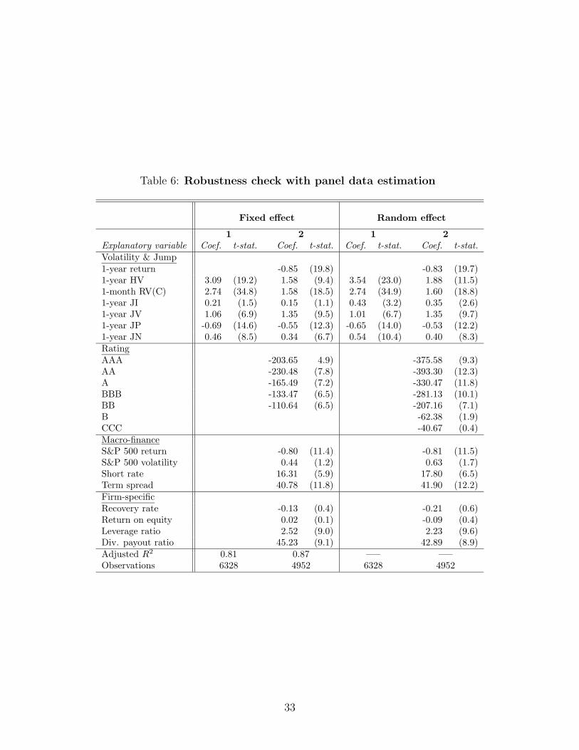
Table 6: Robustness check with panel data estimation
Fixed effect Random effect
1 2 1 2Explanatory variable Coef. t-stat. Coef. t-stat. Coef. t-stat. Coef. t-stat.
Volatility & Jump1-year return -0.85 (19.8) -0.83 (19.7)1-year HV 3.09 (19.2) 1.58 (9.4) 3.54 (23.0) 1.88 (11.5)1-month RV(C) 2.74 (34.8) 1.58 (18.5) 2.74 (34.9) 1.60 (18.8)1-year JI 0.21 (1.5) 0.15 (1.1) 0.43 (3.2) 0.35 (2.6)1-year JV 1.06 (6.9) 1.35 (9.5) 1.01 (6.7) 1.35 (9.7)1-year JP -0.69 (14.6) -0.55 (12.3) -0.65 (14.0) -0.53 (12.2)1-year JN 0.46 (8.5) 0.34 (6.7) 0.54 (10.4) 0.40 (8.3)RatingAAA -203.65 4.9) -375.58 (9.3)AA -230.48 (7.8) -393.30 (12.3)A -165.49 (7.2) -330.47 (11.8)BBB -133.47 (6.5) -281.13 (10.1)BB -110.64 (6.5) -207.16 (7.1)B -62.38 (1.9)CCC -40.67 (0.4)Macro-financeS&P 500 return -0.80 (11.4) -0.81 (11.5)S&P 500 volatility 0.44 (1.2) 0.63 (1.7)Short rate 16.31 (5.9) 17.80 (6.5)Term spread 40.78 (11.8) 41.90 (12.2)Firm-specificRecovery rate -0.13 (0.4) -0.21 (0.6)Return on equity 0.02 (0.1) -0.09 (0.4)Leverage ratio 2.52 (9.0) 2.23 (9.6)Div. payout ratio 45.23 (9.1) 42.89 (8.9)Adjusted R2 0.81 0.87 —– —–Observations 6328 4952 6328 4952
33

Table 7: Regressions by rating groups
Group 1 Group 2 Group 3
(AAA, AA, and A) (BBB) (High-yield)Explanatory variable Coef. t-stat. Coef. t-stat. Coef. t-stat.
Volatility & JumpConstant -109.87 (8.0) -347.00 (9.7) -351.10 (2.8)1-year return -0.12 (3.5) -0.61 (9.3) -0.76 (5.9)1-year HV 0.75 (6.8) 3.81 (17.8) 3.25 (8.3)1-month RV(C) 0.36 (5.8) 1.38 (9.9) 2.17 (6.5)1-year JI 0.24 (3.6) 0.30 (2.6) 1.52 (4.4)1-year JV -0.03 (0.3) 0.06 (0.2) 3.55 (9.4)1-year JP -0.13 (4.0) -0.31 (5.6) -1.10 (9.0)1-year JN 0.13 (4.7) 0.60 (9.4) 0.52 (4.3)Macro-financeS&P 500 return -0.41 (9.4) -1.29 (11.4) -1.69 (4.0)S&P 500 volatility 0.54 (2.5) 0.31 (0.5) 6.46 (3.0)Short rate 9.95 (6.1) 14.48 (3.4) -12.12 (0.7)Term spread 19.03 (9.2) 48.02 (8.8) 59.10 (2.9)Firm-specificRecovery rate 0.61 (3.0) 1.11 (2.2) -5.32 (3.8)Return on equity -1.19 (9.5) -1.85 (5.9) 1.23 (1.4)Leverage ratio 0.20 (5.5) 0.54 (4.3) 5.19 (11.1)Div. payout ratio 16.45 (8.1) 24.17 (6.1) 59.83 (3.6)Adjusted R2 0.41 0.54 0.65Observations 1881 2311 760
34

Table 8: Nonlinear effects of equity volatilities and jumps
Explanatory variable Coef. t-stat.
Volatility & Jump1-year return -0.73 (15.8)HV -5.47 (6.8)HV2 2.04 (11.7)HV3 -0.13 (12.4)RV(C) -1.60 (4.2)RV(C)2 0.44 (7.1)RV(C)3 -0.01 (3.9)JI 0.68 (1.5)JI2 -0.09 (1.2)JI3 0.006 (1.2)JV -0.14 (0.3)JV2 0.27 (3.1)JV3 -0.01 (2.8)JP 0.02 (0.1)JP2 -0.04 (3.2)JP3 0.0007 (2.7)JN 0.02 (0.1)JN2 0.06 (4.8)JN3 -0.002 (5.5)RatingAAA -134.10 (4.2)AA -128.08 (4.2)A -112.64 (3.8)BBB -49.84 (1.7)BB 159.28 (5.2)B 300.55 (9.7)CCC 282.89 (5.8)Macro-financeS&P 500 return -0.97 (10.8)S&P 500 volatility 2.04 (4.47)3M Treasury rate 16.26 (4.9)Term spread 40.48 (9.6)Firm-specificRecovery rate -0.44 (1.2)Return on equity -0.91 (3.9)Leverage ratio 0.69 (8.2)Div. payout ratio 18.22 (5.4)Adjusted R2 0.80Observations 4952
35
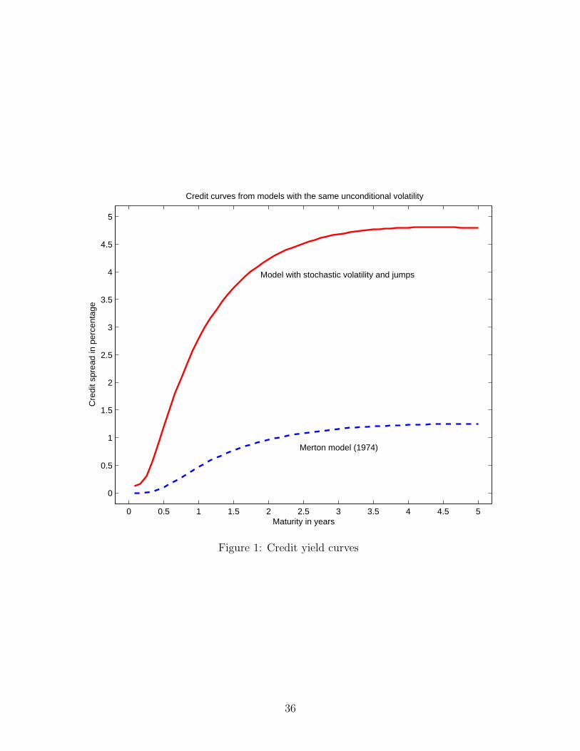
0 0.5 1 1.5 2 2.5 3 3.5 4 4.5 5
0
0.5
1
1.5
2
2.5
3
3.5
4
4.5
5
Maturity in years
Cre
dit s
prea
d in
per
cent
age
Merton model (1974)
Model with stochastic volatility and jumps
Credit curves from models with the same unconditional volatility
Figure 1: Credit yield curves
36

0 1 2 3 4 50
2
4
6
8
10
12
Volatility state Vt1/2
Maturity in years
Cre
dit s
prea
d in
per
cent
age
V1/2t
= 10%
V1/2t
= 30%
V1/2t
= 50%
0 1 2 3 4 50
2
4
6
8
10
12Volatility persistence κ
Maturity in years
Cre
dit s
prea
d in
per
cent
age
κ = 1.6
κ = 2.0
κ = 2.4
0 1 2 3 4 50
2
4
6
8
10
12Volatility long−run mean θ
Maturity in years
Cre
dit s
prea
d in
per
cent
age
θ = 0.01
θ = 0.09
θ = 0.25
0 1 2 3 4 50
2
4
6
8
10
12Volatility−of−volatility σ
Maturity in years
Cre
dit s
prea
d in
per
cent
age
σ = 0.05
σ = 0.4σ = 1.6
0 1 2 3 4 50
2
4
6
8
10
12Volatility asset correlation ρ
Maturity in years
Cre
dit s
prea
d in
per
cent
age
ρ = 1
ρ = −0.6
ρ = −1
0 1 2 3 4 50
2
4
6
8
10
12
Jump size mean µJ
Maturity in years
Cre
dit s
prea
d in
per
cent
age
µJ = 0.00
µJ =−0.95
µJ = 0.95
Figure 2: Comparative statics with volatility and jump parameters
37

0 0.05 0.1 0.15 0.2
4.4
4.6
4.8
5
5.2
5.4
Asset volatility Vt1/2
5−ye
ar c
redi
t spr
ead
0 0.2 0.4 0.6 0.8 1
5
6
7
8Asset jump intensity λ
5−ye
ar c
redi
t spr
ead
−0.2 0 0.2
4.8
4.85
4.9
4.95
Asset jump mean µJ
5−ye
ar c
redi
t spr
ead
0.2 0.4 0.64.6
4.8
5
Asset jump volatility σJ
5−ye
ar c
redi
t spr
ead
0.2 0.3 0.4 0.5 0.6
4.4
4.6
4.8
5
5.2
5.4
Equity volatility Σts
5−ye
ar c
redi
t spr
ead
0 0.2 0.4 0.6 0.8 1
5
6
7
8Equity jump intensity λs
5−ye
ar c
redi
t spr
ead
−0.8 −0.6 −0.4 −0.2 0 0.2
4.8
4.85
4.9
4.95
Equity jump mean µJs
5−ye
ar c
redi
t spr
ead
0.2 0.4 0.6 0.8 1 1.24.6
4.8
5
Equity jump volatility σJs
5−ye
ar c
redi
t spr
ead
Figure 3: Linkages from asset and equity values to credit spreads
38
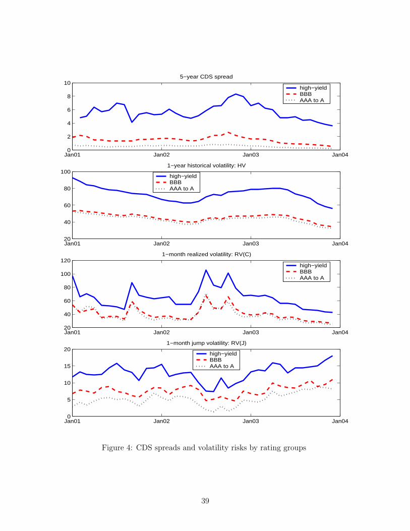
Jan01 Jan02 Jan03 Jan040
2
4
6
8
105−year CDS spread
high−yieldBBBAAA to A
Jan01 Jan02 Jan03 Jan0420
40
60
80
1001−year historical volatility: HV
high−yieldBBBAAA to A
Jan01 Jan02 Jan03 Jan0420
40
60
80
100
1201−month realized volatility: RV(C)
high−yieldBBBAAA to A
Jan01 Jan02 Jan03 Jan040
5
10
15
201−month jump volatility: RV(J)
high−yieldBBBAAA to A
Figure 4: CDS spreads and volatility risks by rating groups
39

20 40 60 80−1
−0.5
0
0.5
1
1.51−year historical volatility HV
Effe
ct o
n cr
edit
spre
ads
0 20 40 60 80 100−0.4
−0.2
0
0.2
0.4
0.61−month realized volatility RV(C)
Effe
ct o
n cr
edit
spre
ads
0 50 100 1500
0.1
0.2
0.3
0.41−year jump intensity JI
Effe
ct o
n cr
edit
spre
ads
0 20 40 60−0.1
0
0.1
0.2
0.3
0.41−year jump volatility JV
Effe
ct o
n cr
edit
spre
ads
−300 −200 −100 0 100 200 300−2
−1
0
1
2
3
41−year signed jumps JP and JN
Effe
ct o
n cr
edit
spre
ads
Figure 5: Nonlinear effects of volatility and jump
The illustration is based on the regression 1 in Table 8. X-axis variables have the value rangeof 5th and 95th percentiles.
40