explaining ligo’s observations via isolated binary ... · explaining ligo’s observations via...
TRANSCRIPT
Explaining LIGO’s observations via isolated binary evolution with natal kicks
Daniel Wysocki,1, ∗ Davide Gerosa,2 Richard O’Shaughnessy,1 Krzysztof Belczynski,3
Wojciech Gladysz,4 Emanuele Berti,5, 6 Michael Kesden,7 and Daniel E. Holz8, 9
1Rochester Institute of Technology, Rochester, New York 14623, USA2TAPIR 350-17, California Institute of Technology,
1200 E California Boulevard, Pasadena, California 91125, USA3Nicolaus Copernicus Astronomical Centre, Polish Academy of Sciences, Ulica Bartycka 18, 00-716 Warsaw, Poland
4Astronomical Observatory, Warsaw University, Aleje Ujazdowskie 4, 00-478 Warsaw, Poland5Department of Physics and Astronomy, The University of Mississippi, University, Mississippi 38677, USA
6CENTRA, Departamento de Fısica, Instituto Superior Tecnico,Universidade de Lisboa, Avenida Rovisco Pais 1, 1049 Lisboa, Portugal
7Department of Physics, The University of Texas at Dallas, Richardson, Texas 75080, USA8Enrico Fermi Institute, Department of Physics, Department of Astronomy and Astrophysics,
and Kavli Institute for Cosmological Physics, University of Chicago, Chicago, Illinois 60637, USA9Kavli Institute for Particle Astrophysics & Cosmology and Physics Department,
Stanford University, Stanford, California 94305, USA(Dated: June 22, 2018)
We compare binary evolution models with different assumptions about black-hole natal kicks tothe first gravitational-wave observations performed by the LIGO detectors. Our comparisons attemptto reconcile merger rate, masses, spins, and spin-orbit misalignments of all current observations withstate-of-the-art formation scenarios of binary black holes formed in isolation. We estimate that blackholes (BHs) should receive natal kicks at birth of the order of σ ' 200 (50) km/s if tidal processes do(not) realign stellar spins. Our estimate is driven by two simple factors. The natal kick dispersion σ isbounded from above because large kicks disrupt too many binaries (reducing the merger rate belowthe observed value). Conversely, the natal kick distribution is bounded from below because modestkicks are needed to produce a range of spin-orbit misalignments. A distribution of misalignmentsincreases our models’ compatibility with LIGO’s observations, if all BHs are likely to have natalspins. Unlike related work which adopts a concrete BH natal spin prescription, we explore a rangeof possible BH natal spin distributions. Within the context of our models, for all of the choices of σused here and within the context of one simple fiducial parameterized spin distribution, observationsfavor low BH natal spin.
I. INTRODUCTION
The discovery and interpretation of gravitational waves(GW) from coalescing binaries [1] has initiated a revolu-tion in astronomy [2]. Several hundred more detectionsare expected over the next five years [3–5]. Already, theproperties of the sources responsible—the inferred eventrates, masses, and spins—have confronted other obser-vations of black hole (BH) masses and spins [4], chal-lenged previous formation scenarios [2, 4], and inspirednew models [6–9] and insights [10, 11] into the evolutionof massive stars and the observationally accessible grav-itational waves they emit [12, 13]. Over the next severalyears, our understanding of the lives and deaths of mas-sive stars over cosmic time will be transformed by theidentification and interpretation of the population(s) re-sponsible for coalescing binaries, with and without coun-terparts, because measurements will enable robust teststo distinguish between formation scenarios with present[14, 15] and future instruments [16, 17], both coarselyand with high precision. In this work, we demonstrate thepower of gravitational wave measurements to constrain
how BHs form, within the context of one formation sce-nario for binary BHs: the isolated evolution of pairs ofstars [18–28].
Within the context of that model, we focus our at-tention on the one feature whose unique impacts mightbe most observationally accessible: BH natal kicks. Ob-servations strongly suggest that when compact objectslike neutron stars are formed after the death of a mas-sive star, their birth can impart significant linear mo-mentum or “kick.” For example, observations of pulsarsin our galaxy suggest birth velocity changes as high asvk ∼ 450 km/s [29]. These impulsive momentum changesimpact the binary’s intrinsic orbit and stability, chang-ing the orbital parameters like semimajor axis and orbitalplane [30, 31], as well as causing the center of mass of theremnant BH binary (if still bound) to recoil at a smallerbut still appreciable velocity. While no single compellingand unambiguous observation can be explained only witha BH natal kick, the assumption of small but nonzeroBH natal kicks provides a natural explanation for severalobservations, including the posterior spin-orbit misalign-ment distribution of GW151226 and the galactic x-raybinary misalignment [32–35] and recoil velocity [36–41].Modest BH natal kicks can be produced by, for example,suitable neutrino-driven supernova engines; see, e.g., [42]and references therein.
arX
iv:1
709.
0194
3v3
[as
tro-
ph.H
E]
20
Jun
2018
2
We compare binary formation models with differentBH natal kick prescriptions to LIGO observations of bi-nary black holes. Along with [42], our calculation is oneof the first to perform this comparison while changinga single, physically well-defined and astrophysically in-teresting parameter: the BH natal kick strength. It isthe first to self-consistently draw inferences about binaryevolution physics by comparing observations simultane-ously to the predicted detection rate; binary BH masses;and binary BH spins, accounting for both magnitude andmisalignment.
This comparison is important because BH natal kicksintroduce two complementary and unusually distinctiveeffects on the binary BHs that LIGO detects. On the onehand, strong BH natal kicks will frequently disrupt pos-sible progenitor binary systems. As the strength of BHnatal kicks increases, the expected number of coalescingbinary BHs drops precipitously [19, 20, 43]. On the ba-sis of observations to date, BH natal kicks drawn froma distribution with one-dimensional velocity dispersion σgreater than 265 km/s are disfavored [26]. On the otherhand, BH natal kicks will tilt the orbital plane, misalign-ing the orbital angular momentum from the black hole’snatal spin direction—assumed parallel to the progenitorbinary’s orbital angular momentum [15, 31]. The imprintof these natal kicks on the binary’s dynamics is preservedover the aeons between the BH-BH binary’s formationand its final coalescence [30, 44–46]. The outgoing radi-ation from each merger contains information about thecoalescing binary’s spin (see, e.g., [47–49] and referencestherein), including conserved constants that directly re-flect the progenitor binary’s state [50, 51]. Several stud-ies have demonstrated that the imprint of processes thatmisalign BH spins and the orbit can be disentangled [52–54].
In this work, we show that LIGO’s observations of bi-nary black holes can be easily explained in the contextof isolated binary evolution, if BH natal kicks act withthe (modest) strength to misalign the orbital plane fromthe initial spin directions (presumed aligned). In this ap-proach, the absence of large aligned spins either reflectsfortuitous but nonrepresentative observations or low na-tal BH spins. A companion study by Belczynski et al. [42]describes an alternative, equally plausible explanation:the BH natal spin depends on the progenitor, such thatthe most massive BHs are born with low natal spins. Alonger companion study by Gerosa et al. [55] will describethe properties and precessing dynamics of this populationin greater detail.
This paper is organized as follows. First, in Sec. II wedescribe the entire process used to generate and char-acterize detection-weighted populations of precessing bi-nary BHs, evaluated using different assumptions aboutBH natal kicks. As described in Sec. II A, we adopt pre-viously studied binary evolution calculations to deter-mine how frequently compact binaries merge throughoutthe universe. In Sec. II B, we describe how we evolve thebinary’s precessing BH spins starting from just after it
forms until it enters the LIGO band. In Sec. II C, we de-scribe the parameters we use to characterize each binary:the component masses and spins, evaluated after evolv-ing the BH binary according to the process describedin Sec. II B. To enable direct comparison with observa-tions, we convert from detection-weighted samples—theoutput of our binary evolution model—to a smoothedapproximation, allowing us to draw inferences about therelative likelihood of generic binary parameters. In Sec.III we compare these smoothed models for compact bi-nary formation against LIGO’s observations to date. Wesummarize our conclusions in Sec. VI. In Appendix A wedescribe the technique we use to approximate each of ourbinary evolution simulations. In Appendix B, we providetechnical details of the underlying statistical techniqueswe use to compare these approximations to LIGO obser-vations. To facilitate exploration of alternative assump-tions about natal spins and kicks, we have made publiclyavailable all of the marginalized likelihoods evaluated inthis work, as Supplemental material [56].
II. ESTIMATING THE OBSERVEDPOPULATION OF COALESCING BINARY
BLACK HOLES
A. Forming compact binaries over cosmic time
Our binary evolution calculations are performed withthe StarTrack isolated binary evolution code [20, 58],with updated calculation of common-envelope physics[23], compact remant masses [59], and pair instabilitysupernovae [57]. Using this code, we generate a syntheticuniverse of (weighted) binaries by Monte Carlo [24]. Ourcalculations account for the time- and metallicity- de-pendent star formation history of the universe, by us-ing a grid of 32 different choices for stellar metallicity.As shown in Table I, we create synthetic universes us-ing the same assumptions (M10) adopted by default inprevious studies [26, 42, 57]. Again as in previous work,we explore a one-parameter family of simulations thatadopt different assumptions about BH natal kicks (M13-M18). Each new model assumes all BHs receive natalkicks drawn from the same Maxwellian distribution, withone-dimensional velocity distribution parameterized by σ(a quantity which changes from model to model). In theM10 model used for reference, BH kicks are also drawnfrom a Maxwellian distribution, but suppressed by thefraction of ejected material that is retained (i.e., does notescape to infinity, instead being accreted by the BH). Be-cause the progenitors of the most massive BHs do not,in our calculations, eject significant mass to infinity, theheaviest BHs formed in this “fallback-suppressed kick”scenario receive nearly or exactly zero natal kicks.
These synthetic universes consist of weighted BH-BHmergers (indexed by i), each one acting a proxy for apart of the overall merger rate density in its local volume[25, 39]. As our synthetic universe resamples from the
3
Name σ (km/s) DKL(M) DKL(m1,m2)
M10 Ø 0.02 0.21
M18 25 0.006 0.094
M17 50 0 0
M16 70 0.016 0.28
M15 130 0.1 1.26
M14 200 0.17 1.56
M13 265 0.40 2.1
TABLE I. Properties of the formation scenarios adopted inthis work. The first column indicates the model calculationname, using the convention of other work [26, 57]. The secondcolumn provides the kick distribution width. Model M10adopts mass-dependent, fallback suppressed BH natal kicks.For the BH population examined here, these natal kicks areeffectively zero for massive BHs; see, e.g., [14]. The remainingscenarios adopt a mass-independent Maxwellian natal kickdistribution characterized by the 1-d velocity dispersion σ, asdescribed in the text. The third column quantifies how muchthe mass distribution changes as we change σ. To be concrete,we compare the (source frame) total mass distributions forthe BH-BH binaries LIGO is expected to detect, usinga Kullback–Leibler (KL) divergence [Eq. (4)]. If p(M |α)denotes the mass distribution for α = M10, M18, M17,. . ., and α∗ denotes M17, then the third column is the KLdivergence DKL(M,α) =
∫dMp(M |α) ln[p(M |α)/p(M |α∗)].
The fourth column is the KL divergence using the jointdistribution of both binary masses: DKL(m1,m2|α) =∫dm1dm2p(m1,m2|α) ln[p(m1,m2|α)/p(m1,m2|α∗)]. Be-
cause M10 adopts fallback-suppressed natal kicks, while theremaining models assume fallback-independent natal kicks,we use the special symbol Ø to refer to M10 in subsequentplots and figures.
same set of 32 choices for stellar metallicity, the sameevolutionary trajectory appears many times, each at dif-ferent redshifts and reflecting the relative probability ofstar formation at different times. The most frequent for-mation scenarios and the fraction of detected binariesfrom each channel are shown in Table II.
The underlying binary evolution calculations per-formed by StarTrack effectively do not depend on BHspins at any stage.1 We therefore have the freedom toreuse each calculation above with any BH natal spin pre-scription whatsoever. Unlike Belczynski et al. [42], wedo not adopt a physically-motivated and mass-dependentBH natal spin, to allow us to explore all of the possibili-
1 The response of the BH’s mass and spin to accretion depends onthe BH’s spin. We adopt a standard procedure whereby the BHaccretes from the innermost stable circular orbit. In our binaryevolution code, this spin evolution is implemented directly viaan ODE based on (prograde, aligned) ISCO accretion as in [60],though the general solution is provided in [61] and applied since,e.g., in [62, 63]. For the purposes of calculating the final BH massfrom the natal mass and its accretion history, we adopted a BHnatal spin of χ = 0.5; however, relatively little mass is accretedand the choice of spin has a highly subdominant effect on theBH’s evolution.
ties that nature might allow. Instead, we treat the birthspin for each BH as a parameter, assigning spins χ1 andχ2 to each black hole at birth. For simplicity and with-out loss of generality, for each event we assume a fixedBH spin for the first-born (χ1 = |S1| /m2
1) and a poten-tially different spin for the second-born (χ2 = |S2| /m2
2)BH. Both choices of fixed spin are parameters. By carry-ing out our calculations on a discrete grid in χ1, χ2 foreach event—here, we use χ1,2 = 0.1 . . . 1—we encompassa wide range of possible choices for progenitor spins, al-lowing us to explore arbitrary (discrete) natal spin distri-butions. For comparison, [53] adopted a fixed natal spinχi = 0.7 for all BHs. Our choices for BH natal spin distri-butions are restricted only by our choice of discrete spins.Our model is also implicitly limited by requiring all BHshave natal spins drawn from the same mass-independentdistributions. By design, our calculation did not includeenough degrees of freedom to enable the natal spin dis-tribution to change with mass, as was done for examplein [42].
We assume the progenitor stellar binary is comprisedof stars whose spin axes are aligned with the orbital an-gular momentum, reflecting natal or tidal [64, 65] align-ment (but cf. [66]). After the first supernova, several pro-cesses could realign the stellar or BH spin with the or-bital plane, including mass accretion onto the BH andtidal dissipation in the star. Following Gerosa et al. [30],we consider two possibilities. In our default scenario (“notides”), spin-orbit alignment is only influenced by BH na-tal kicks. In the other scenario (“tides”), tidal dissipationwill cause the stellar spin in stellar-BH binaries to alignparallel to the orbital plane. In the “tides” scenario, thesecond-born stellar spin is aligned with the orbital an-gular momentum prior to the second SN. Following [30],the “tides” scenario assumes alignment always occurs formerging BH-BH binaries, independent of the specific evo-lutionary trajectory involved (e.g., binary separation); cf.the discussion in [42]. In both formation scenarios, wedo not allow mass accretion onto the BH to change theBH’s spin direction. Given the extremely small amountof mass accreted during either conventional or common-envelope mass transfer, even disk warps and the Bardeen-Petterson effect should not allow the BH spin direction toevolve [67–70]. For coalescing BH-BH binaries the secondSN often occurs when the binary is in a tight orbit, withhigh orbital speed, and thus less effect on spin-orbit mis-alignment [15, 31]. Therefore, in the “tides” scenario, thesecond-born BH’s spin is more frequently nearly alignedwith the final orbital plane, even for large BH natal kicks.
B. Evolving from birth until merger
The procedure above produces a synthetic universeof binary BHs, providing binary masses, spins, and or-bits just after the second BH is born. Millions to bil-lions of years must pass before these binaries coalesce,during which time the orbital and BH spin angular mo-
4
Formation mechanism Fraction
MT1(2-1) MT1(4-1) SN1 CE2(14-4;14-7) SN2 0.261
MT1(4-4) CE2(7-4;7-7) SN1 SN2 0.234
MT1(4-1) SN1 CE2(14-4;14-7) SN2 0.140
MT1(2-1) SN1 CE2(14-4;14-7) SN2 0.075
MT1(4-4) CE2(4-4;7-7) SN1 SN2 0.071
MT1(2-1) SN1 MT2(14-2) SN2 0.037
CE1(4-1;7-1) SN1 MT2(14-2) SN2 0.028
CE1(4-1;7-1) SN1 CE2(14-4;14-7) SN2 0.020
CE1(4-1;7-1) CE2(7-4;7-7) SN1 SN2 0.014
MT1(4-4) CE12(4-4;7-7) SN2 SN1 0.014
SN1 CE2(14-4;14-7) SN2 0.014
Other channels 0.16
TABLE II. The most significant formation scenarios and frac-tion of detected binaries formed from that channel, for theM15 model. While many of the coalescing BH-BH binariesform via a BH-star binary undergoing some form of stellarmass transfer or interaction, a significant fraction of binariesform without any Roche lobe overflow mass transfer after thefirst SN. In this example, in the second channel alone morethan 23% of binaries form without interaction after the firstSN. (The remaining formation channels account for 16% ofthe probability.) In this notation, integers in braces charac-terize the types of the stellar system in the binary; the pre-fix refers to different phases of stellar interaction (e.g., MTdenotes “mass transfer,” SN denotes “supernova,” and CEdenotes “common envelope evolution”); and the last integerSNx indicates whether the initial primary star (1) or initialsecondary star (2) has collapsed and/or exploded to form aBH. [Some of our BHs are formed without luminous explo-sions; we use SN to denote the death of a massive star andthe formation of a compact object.] A detailed descriptionof these formation channels and stellar types notation is pro-vided in [20, 58]; in this shorthand, 1 denotes a main sequencestar; 2 denotes a Hertzprung gap star; 4 denotes a core heliumburning star; 7 denotes a main sequence naked helium star;and 14 denotes a black hole.
menta precess substantially [45, 46]. We use precession-averaged 2PN precessional dynamics, as implementedin precession [71], to evolve the spins from birth un-til the binary BH orbital frequency is 10Hz (i.e., un-til the GW frequency is 20Hz); see [55] for details.When identifying initial conditions, we assume the bi-nary has already efficiently circularized. When identi-fying the final separation, we only use the Newtonian-order relationship between separation and orbital fre-quency. The precession code is publicly available atgithub.com/dgerosa/precession.
C. Characterizing the observed distribution ofbinaries
At the fiducial reference frequency adopted in this work(20Hz), a binary BH is characterized by its componentmasses and its (instantaneous) BH spins S1,2. For the
heavy BHs of current interest to LIGO, the principal ef-fect of BH spin on the orbit and emitted radiation occursthrough the spin combination
χeff = (S1/m1 + S2/m2) · L/(m1 +m2)
= (χ1m1 cos θ1 + χ2m2 cos θ2)/(m1 +m2), (1)
where θ1,2 denote the angles between the orbital angu-lar momentum and the component BH spins. That said,depending on the duration and complexity of the sourceresponsible, GW measurements may also provide addi-tional constraints on the underlying spin directions them-selves [50], including on the spin-orbit misalignment an-gles θ1,2. For the purposes of this work, we will be in-terested in the (source-frame) binary masses m1,m2 andthe spin parameters χeff , θ1, θ2, as an approximate char-acterization of the most observationally accessible de-grees of freedom; cf. Stevenson et al. [53], which usedθ1,2, and Trifiro et al. [50], which used θ1,2 and the angle∆Φ between the spins’ projection onto the orbital plane.In particular, ∆Φ is well-known to contain valuable in-formation [30] and be observationally accessible [50]. Atpresent, the preferred model adopted for parameter infer-ence, known as IMRPhenomP, does not incorporate thenecessary degree of freedom [72], so we cannot incorpo-rate its effect here. With additional and more informa-tive binary black hole observations, however, our methodshould be extended to employ all of the spin degrees offreedom, particularly ∆Φ. As input, this extension willrequire inference results that incorporate the effect of twotwo precessing spins, either by using semianalytical mod-els [73–75] or by using numerical relativity [49].
We adopt a conventional model for LIGO’s sensitiv-ity to a population of binary BHs [3, 25, 76]. In thisapproach, LIGO’s sensitivity is limited by the second-most-sensitive interferometer, using a detection thresh-old signal-to-noise ratio ρ = 8 and the fiducial detectorsensitivity reported for O1 [4]. This sensitivity model isa good approximation to the performance reported forboth in O1 and early in O2 [5]. Following [25, 39], we usethe quantity ri [Eq. (8) in [39]] to account for the con-tribution of this binary to LIGO’s detection rate in oursynthetic universe, accounting for the size of the universeat the time the binary coalesces and LIGO’s orientation-dependent sensitivity. For simplicity and following pre-vious work [3, 25], we estimate the detection probabilitywithout accounting for the effects of BH spin. Previousstudies have used this detection-weighted procedure toevaluate and report on the expected distribution of bi-nary BHs detected by LIGO [26, 42, 57]. Since the samebinary evolution A occurs many times in our syntheticuniverse, we simplify our results by computing one over-all detection rate rA =
∑i∈A ri for each evolution. When
this procedure is performed, relatively few distinct binaryevolutions A have significant weight. While our syntheticuniverse contains millions of binaries, only O(104) dis-tinct BH-BH binaries are significant in our final resultsfor each of the formation scenarios listed in Table I. Fig. 1illustrates the expected detected number versus assumed
5
Ø 25 50 70 130 200 265
σkick [km s−1]
0
5
10
15
20
25ex
pec
tedN
even
ts
Observed
M10 M18 M17M16 M15 M14 M13
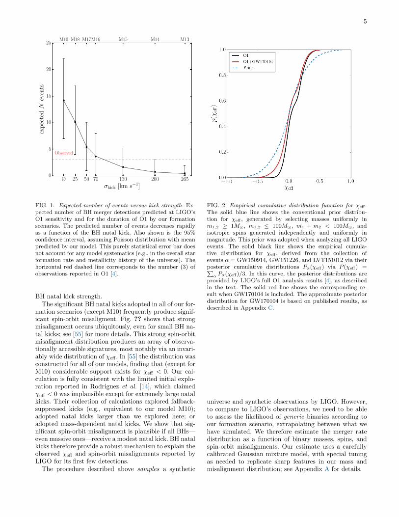
FIG. 1. Expected number of events versus kick strength: Ex-pected number of BH merger detections predicted at LIGO’sO1 sensitivity and for the duration of O1 by our formationscenarios. The predicted number of events decreases rapidlyas a function of the BH natal kick. Also shown is the 95%confidence interval, assuming Poisson distribution with meanpredicted by our model. This purely statistical error bar doesnot account for any model systematics (e.g., in the overall starformation rate and metallicity history of the universe). Thehorizontal red dashed line corresponds to the number (3) ofobservations reported in O1 [4].
BH natal kick strength.The significant BH natal kicks adopted in all of our for-
mation scenarios (except M10) frequently produce signif-icant spin-orbit misaligment. Fig. ?? shows that strongmisalignment occurs ubiquitously, even for small BH na-tal kicks; see [55] for more details. This strong spin-orbitmisalignment distribution produces an array of observa-tionally accessible signatures, most notably via an invari-ably wide distribution of χeff . In [55] the distribution wasconstructed for all of our models, finding that (except forM10) considerable support exists for χeff < 0. Our cal-culation is fully consistent with the limited initial explo-ration reported in Rodriguez et al. [14], which claimedχeff < 0 was implausible except for extremely large natalkicks. Their collection of calculations explored fallback-suppressed kicks (e.g., equivalent to our model M10);adopted natal kicks larger than we explored here; oradopted mass-dependent natal kicks. We show that sig-nificant spin-orbit misalignment is plausible if all BHs—even massive ones—receive a modest natal kick. BH natalkicks therefore provide a robust mechanism to explain theobserved χeff and spin-orbit misalignments reported byLIGO for its first few detections.
The procedure described above samples a synthetic
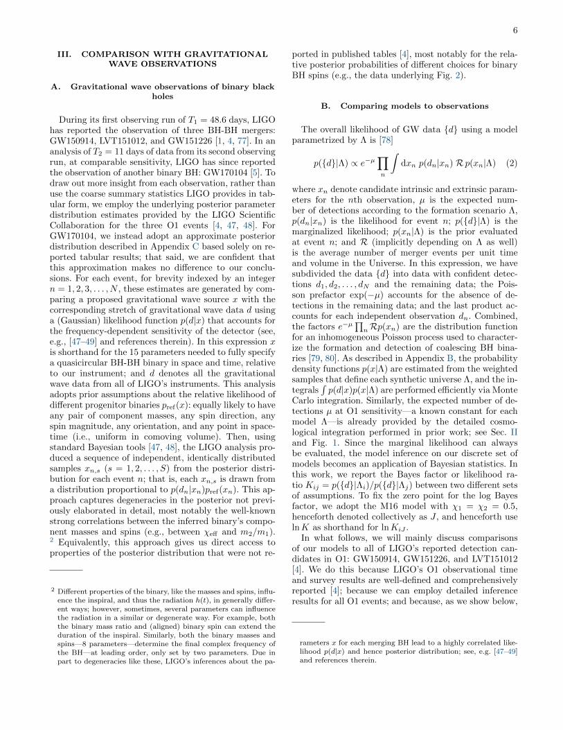
FIG. 2. Empirical cumulative distribution function for χeff :The solid blue line shows the conventional prior distribu-tion for χeff , generated by selecting masses uniformly inm1,2 ≥ 1M�, m1,2 ≤ 100M�, m1 + m2 < 100M�, andisotropic spins generated independently and uniformly inmagnitude. This prior was adopted when analyzing all LIGOevents. The solid black line shows the empirical cumula-tive distribution for χeff , derived from the collection ofevents α = GW150914, GW151226, and LVT151012 via theirposterior cumulative distributions Pα(χeff) via P (χeff) =∑α Pα(χeff)/3. In this curve, the posterior distributions are
provided by LIGO’s full O1 analysis results [4], as describedin the text. The solid red line shows the corresponding re-sult when GW170104 is included. The approximate posteriordistribution for GW170104 is based on published results, asdescribed in Appendix C.
universe and synthetic observations by LIGO. However,to compare to LIGO’s observations, we need to be ableto assess the likelihood of generic binaries according toour formation scenario, extrapolating between what wehave simulated. We therefore estimate the merger ratedistribution as a function of binary masses, spins, andspin-orbit misalignments. Our estimate uses a carefullycalibrated Gaussian mixture model, with special tuningas needed to replicate sharp features in our mass andmisalignment distribution; see Appendix A for details.
6
III. COMPARISON WITH GRAVITATIONALWAVE OBSERVATIONS
A. Gravitational wave observations of binary blackholes
During its first observing run of T1 = 48.6 days, LIGOhas reported the observation of three BH-BH mergers:GW150914, LVT151012, and GW151226 [1, 4, 77]. In ananalysis of T2 = 11 days of data from its second observingrun, at comparable sensitivity, LIGO has since reportedthe observation of another binary BH: GW170104 [5]. Todraw out more insight from each observation, rather thanuse the coarse summary statistics LIGO provides in tab-ular form, we employ the underlying posterior parameterdistribution estimates provided by the LIGO ScientificCollaboration for the three O1 events [4, 47, 48]. ForGW170104, we instead adopt an approximate posteriordistribution described in Appendix C based solely on re-ported tabular results; that said, we are confident thatthis approximation makes no difference to our conclu-sions. For each event, for brevity indexed by an integern = 1, 2, 3, . . . , N , these estimates are generated by com-paring a proposed gravitational wave source x with thecorresponding stretch of gravitational wave data d usinga (Gaussian) likelihood function p(d|x) that accounts forthe frequency-dependent sensitivity of the detector (see,e.g., [47–49] and references therein). In this expression xis shorthand for the 15 parameters needed to fully specifya quasicircular BH-BH binary in space and time, relativeto our instrument; and d denotes all the gravitationalwave data from all of LIGO’s instruments. This analysisadopts prior assumptions about the relative likelihood ofdifferent progenitor binaries pref(x): equally likely to haveany pair of component masses, any spin direction, anyspin magnitude, any orientation, and any point in space-time (i.e., uniform in comoving volume). Then, usingstandard Bayesian tools [47, 48], the LIGO analysis pro-duced a sequence of independent, identically distributedsamples xn,s (s = 1, 2, . . . , S) from the posterior distri-bution for each event n; that is, each xn,s is drawn froma distribution proportional to p(dn|xn)pref(xn). This ap-proach captures degeneracies in the posterior not previ-ously elaborated in detail, most notably the well-knownstrong correlations between the inferred binary’s compo-nent masses and spins (e.g., between χeff and m2/m1).2 Equivalently, this approach gives us direct access toproperties of the posterior distribution that were not re-
2 Different properties of the binary, like the masses and spins, influ-ence the inspiral, and thus the radiation h(t), in generally differ-ent ways; however, sometimes, several parameters can influencethe radiation in a similar or degenerate way. For example, boththe binary mass ratio and (aligned) binary spin can extend theduration of the inspiral. Similarly, both the binary masses andspins—8 parameters—determine the final complex frequency ofthe BH—at leading order, only set by two parameters. Due inpart to degeneracies like these, LIGO’s inferences about the pa-
ported in published tables [4], most notably for the rela-tive posterior probabilities of different choices for binaryBH spins (e.g., the data underlying Fig. 2).
B. Comparing models to observations
The overall likelihood of GW data {d} using a modelparametrized by Λ is [78]
p({d}|Λ) ∝ e−µ∏n
∫dxn p(dn|xn) R p(xn|Λ) (2)
where xn denote candidate intrinsic and extrinsic param-eters for the nth observation, µ is the expected num-ber of detections according to the formation scenario Λ,p(dn|xn) is the likelihood for event n; p({d}|Λ) is themarginalized likelihood; p(xn|Λ) is the prior evaluatedat event n; and R (implicitly depending on Λ as well)is the average number of merger events per unit timeand volume in the Universe. In this expression, we havesubdivided the data {d} into data with confident detec-tions d1, d2, . . . , dN and the remaining data; the Pois-son prefactor exp(−µ) accounts for the absence of de-tections in the remaining data; and the last product ac-counts for each independent observation dn. Combined,the factors e−µ
∏nRp(xn) are the distribution function
for an inhomogeneous Poisson process used to character-ize the formation and detection of coalescing BH bina-ries [79, 80]. As described in Appendix B, the probabilitydensity functions p(x|Λ) are estimated from the weightedsamples that define each synthetic universe Λ, and the in-tegrals
∫p(d|x)p(x|Λ) are performed efficiently via Monte
Carlo integration. Similarly, the expected number of de-tections µ at O1 sensitivity—a known constant for eachmodel Λ—is already provided by the detailed cosmo-logical integration performed in prior work; see Sec. IIand Fig. 1. Since the marginal likelihood can alwaysbe evaluated, the model inference on our discrete set ofmodels becomes an application of Bayesian statistics. Inthis work, we report the Bayes factor or likelihood ra-tio Kij = p({d}|Λi)/p({d}|Λj) between two different setsof assumptions. To fix the zero point for the log Bayesfactor, we adopt the M16 model with χ1 = χ2 = 0.5,henceforth denoted collectively as J , and henceforth uselnK as shorthand for lnKiJ .
In what follows, we will mainly discuss comparisonsof our models to all of LIGO’s reported detection can-didates in O1: GW150914, GW151226, and LVT151012[4]. We do this because LIGO’s O1 observational timeand survey results are well-defined and comprehensivelyreported [4]; because we can employ detailed inferenceresults for all O1 events; and because, as we show below,
rameters x for each merging BH lead to a highly correlated like-lihood p(d|x) and hence posterior distribution; see, e.g. [47–49]and references therein.
7
adding GW170104 to our analysis produces little changeto our results. Using the approximate posterior describedin Appendix C for GW170104, we will also compare allreported LIGO observations (O1 and GW170104) to ourmodels.
Critically, for clarity and to emphasize the informa-tion content of the data, in several of our figures we willillustrate the marginal likelihood of the data p({d}|Λ)evaluated assuming all binaries are formed with identi-cal natal spins. These strong assumptions in our illustra-tions show just how much the data informs our under-standing of BH natal spins. With only four observations,assumptions about the spin distribution are critical tomake progress. As described in Appendix B, we can alter-natively evaluate the marginal likelihood accounting forany concrete spin distribution, or even all possible spindistributions—in our context, all possible mixture com-binations of the 100 different choices for χ1 and χ2 thatwe explored. In the latter case, as we show below, just asone expects a priori, observations cannot significantly in-form this 100-dimensional posterior spin distribution. Assuggested in previous studies [e.g. 2, 42, 49, 54], LIGO’sobservations in O1 and O2 can be fit by models thatincludes a wide range of progenitor spins, so long as suf-ficient probability exists for small natal spin and/or sig-nificant misalignment. As a balance between completegenerality on the one hand (a 100-dimensional distribu-tion of natal spin distributions) and implausibly rigid as-sumptions on the other (fixed natal spins), we emphasizea simple one-parameter model, where BH natal spins χare drawn from the piecewise constant distribution
p(χ) =
{λA/0.6 χ ≤ 0.6
(1− λA)/0.4 0.6 < χ < 1(3)
where λA is the probability of a natal spin ≤ 0.6 and thechoice of cutoff 0.6 is motivated by our results below.
IV. RESULTS
In this section we calculate the Bayes factor lnK foreach of the binary evolution models described above. Un-less otherwise noted, we compare our models to LIGO’sO1 observations (i.e., the observation of GW150914,GW151226, and LVT151012), using each model’s corre-lated predictions for the event rate, joint mass distribu-tion (m1,m2), χeff distribution, and the distribution ofθ1, θ2. For numerical context, a Bayes factor of ln 10 ' 2.3is by definition equivalent to 10:1 odds in favor of somemodel over our reference model. Bayes factors that aremore than 5 below the largest Bayes factor observed arein effect implausible (e.g., more than 148:1 odds against),whereas anything within 2 of the peak are reasonablylikely.
A. Standard scenario and limits on BH natal spins(O1)
The M10 model allows us to examine the implica-tions of binary evolution with effectively zero natal kicks.The M10 model adopts fiducial assumptions about bi-nary evolution and BH natal kicks, as described in priorwork [26, 57]. In this model, BH kicks are suppressed byfallback; as a result, the heaviest BHs receive nearly orexactly zero natal kicks and hence have nearly or exactlyzero spin-orbit misalignment.
If heavy BH binaries have negligible spin-orbit mis-alignment, then natal BH spins are directly constrainedfrom LIGO’s measurements (e.g., of χeff). For exam-ple, LIGO’s observations of GW150914 severely constrainits component spins to be small, if the spins must bestrictly and positively aligned [48, 49]. Conversely, how-ever, LIGO’s observations for GW151226 require somenonzero spin. Combined, if we assume all BHs have spinsdrawn from the same, mass-independent distribution andhave negligible spin-orbit misalignments, then we con-clude BH natal spins should be preferentially small. [Wewill return to this statement in Sec. IV D.]
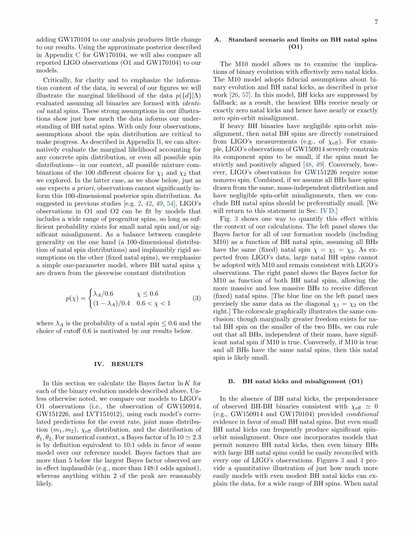
Fig. 3 shows one way to quantify this effect withinthe context of our calculations. The left panel shows theBayes factor for all of our formation models (includingM10) as a function of BH natal spin, assuming all BHshave the same (fixed) natal spin χ = χ1 = χ2. As ex-pected from LIGO’s data, large natal BH spins cannotbe adopted with M10 and remain consistent with LIGO’sobservations. The right panel shows the Bayes factor forM10 as function of both BH natal spins, allowing themore massive and less massive BHs to receive different(fixed) natal spins. [The blue line on the left panel usesprecisely the same data as the diagonal χ1 = χ2 on theright.] The colorscale graphically illustrates the same con-clusion: though marginally greater freedom exists for na-tal BH spin on the smaller of the two BHs, we can ruleout that all BHs, independent of their mass, have signif-icant natal spin if M10 is true. Conversely, if M10 is trueand all BHs have the same natal spins, then this natalspin is likely small.
B. BH natal kicks and misalignment (O1)
In the absence of BH natal kicks, the preponderanceof observed BH-BH binaries consistent with χeff ' 0(e.g., GW150914 and GW170104) provided conditionalevidence in favor of small BH natal spins. But even smallBH natal kicks can frequently produce significant spin-orbit misalignment. Once one incorporates models thatpermit nonzero BH natal kicks, then even binary BHswith large BH natal spins could be easily reconciled withevery one of LIGO’s observations. Figures 3 and 4 pro-vide a quantitative illustration of just how much moreeasily models with even modest BH natal kicks can ex-plain the data, for a wide range of BH spins. When natal
8
0.0 0.2 0.4 0.6 0.8 1.0χ1 = χ2
−15
−10
−5
0
5lnK
M10
M13
M14
M15
M16
M17
M18
No Tides
Tides0.0 0.2 0.4 0.6 0.8 1.0
χ1
0.0
0.2
0.4
0.6
0.8
1.0
χ2
-3.70
-4.79
-7.04
-10.3
-15.1
-21.3
-28.6
-36.3
-45.4
-55.9
-4.58
-7.17
-11.1
-16.6
-23.4
-30.3
-39.2
-49.8
-60.8
-73.9
-7.45
-11.9
-18.3
-25.9
-34.4
-43.2
-53.9
-66.2
-78.7
-83.8
-13.0
-20.0
-28.4
-38.1
-47.8
-59.2
-70.7
-80.1
-85.5
-85.5
-21.1
-29.9
-40.1
-51.3
-62.9
-76.7
-81.1
-82.7
-87.1
-87.2
-30.5
-41.6
-53.4
-66.6
-80.9
-82.5
-82.4
-88.1
-88.1
-88.6
-41.0
-52.6
-69.5
-83.8
-89.9
-89.5
-89.6
-89.3
-89.5
-89.6
-52.1
-66.7
-86.5
-84.5
-91.0
-91.0
-82.2
-90.9
-90.7
-90.6
-68.1
-85.2
-91.6
-85.8
-91.8
-91.4
-91.9
-91.4
-85.8
-91.9
-86.0
-92.9
-92.5
-92.8
-92.3
-92.6
-92.5
-92.5
-92.1
-103.
−100
−90
−80
−70
−60
−50
−40
−30
−20
−10
lnK
FIG. 3. Standard small-kick scenario (M10) requires small natal BH spin: Left panel: A plot of the Bayes factor K derived bycomparing GW151226, GW150914, and LVT151012 to the M10 (blue) formation scenario, versus the magnitude of assumedBH natal spin χ1 = χ2. All other models are shown for comparison. Colors and numbers indicate the Bayes factor; dark colorsdenote particularly unlikely configurations. Right panel: As before (i.e., for M10), but in two dimensions, allowing the BH natalspins for the primary and secondary BH to be independently selected (but fixed); color indicates the Bayes factor. As thisscenario predicts strictly aligned spins for the heaviest BH-BH binaries, only small BH natal spins are consistent with LIGO’sconstraints on the (aligned) BH spin parameter χeff in O1 (and GW170104); see Abbott, B. P. et al. (LIGO and Virgo ScientificCollaboration) [5, 49] and [54].
kicks greater than 25km/s are included, the BH natalspin is nearly unconstrained. As is particularly apparentin Fig. 4, some natal BH spin is required to reproducethe nonzero spin seen in GW151226.
Larger kicks produce frequent, large spin-orbit mis-alignments and therefore greater consistency with theproperties of all of LIGO’s observed binary BHs. Spin-orbit misalignment is consistent with the spin distribu-tion of GW151226, and helpful to explain the distributionof χeff for LIGO’s other observations. However, largerkicks also disrupt more binaries, substantially decreasingthe overall event rate (see Fig. 1). Fig. 4 illustrates thetradeoff between spin-orbit misalignment and event rate.
C. Tides and realignment (O1)
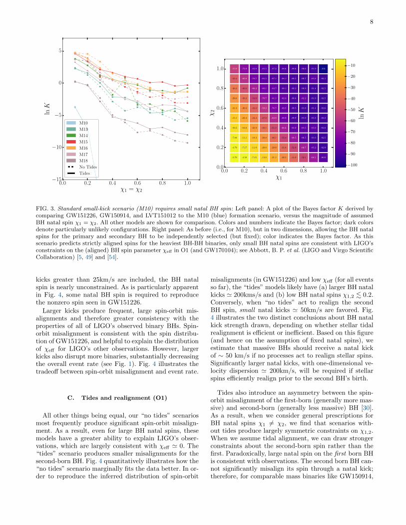
All other things being equal, our “no tides” scenariosmost frequently produce significant spin-orbit misalign-ment. As a result, even for large BH natal spins, thesemodels have a greater ability to explain LIGO’s obser-vations, which are largely consistent with χeff ' 0. The“tides” scenario produces smaller misalignments for thesecond-born BH. Fig. 4 quantitatively illustrates how the“no tides” scenario marginally fits the data better. In or-der to reproduce the inferred distribution of spin-orbit
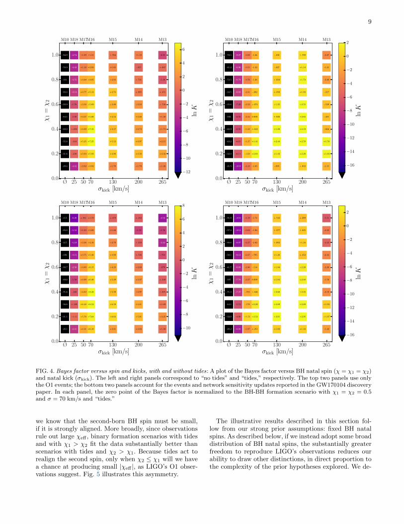
misalignments (in GW151226) and low χeff (for all eventsso far), the “tides” models likely have (a) larger BH natalkicks ' 200kms/s and (b) low BH natal spins χ1,2 . 0.2.Conversely, when “no tides” act to realign the secondBH spin, small natal kicks ' 50km/s are favored. Fig.4 illustrates the two distinct conclusions about BH natalkick strength drawn, depending on whether stellar tidalrealignment is efficient or inefficient. Based on this figure(and hence on the assumption of fixed natal spins), weestimate that massive BHs should receive a natal kickof ∼ 50 km/s if no processes act to realign stellar spins.Significantly larger natal kicks, with one-dimensional ve-locity dispersion ' 200km/s, will be required if stellarspins efficiently realign prior to the second BH’s birth.
Tides also introduce an asymmetry between the spin-orbit misalignment of the first-born (generally more mas-sive) and second-born (generally less massive) BH [30].As a result, when we consider general prescriptions forBH natal spins χ1 6= χ2, we find that scenarios with-out tides produce largely symmetric constraints on χ1,2.When we assume tidal alignment, we can draw strongerconstraints about the second-born spin rather than thefirst. Paradoxically, large natal spin on the first born BHis consistent with observations. The second born BH can-not significantly misalign its spin through a natal kick;therefore, for comparable mass binaries like GW150914,
9
Ø 25 50 70 130 200 265σkick [km/s]
0.0
0.2
0.4
0.6
0.8
1.0
χ1
=χ
2
-29.4
-31.6
-55.8
-69.2
-84.1
-93.9
-93.4
-101.
-78.9
-94.9
+1.26
+3.32
+2.15
+1.73
+1.48
+.746
+.451
-1.36
+.007
-2.25
+1.79
+4.16
+3.97
+2.74
+3.46
+2.24
+.985
+.721
-.457
+1.10
+1.78
+4.86
+5.12
+4.17
+4.54
+3.80
+4.74
+2.83
+1.65
+.784
+3.92
+5.93
+7.25
+7.45
+5.80
+5.69
+5.14
+4.05
+2.93
+1.51
+2.02
+3.93
+5.25
+4.09
+3.57
+3.58
+3.77
+3.44
+1.18
+1.09
-4.41
-.238
-.344
+.004
-1.08
-1.76
-3.14
-3.55
-4.43
-4.74
−12
−10
−8
−6
−4
−2
0
2
4
6
lnK
M10 M18 M17M16 M15 M14 M13
Ø 25 50 70 130 200 265σkick [km/s]
0.0
0.2
0.4
0.6
0.8
1.0
χ1
=χ
2
-21.5
-32.4
-43.2
-68.9
-102.
-35.6
-34.5
-72.5
-41.2
-72.5
-1.15
+1.83
+1.78
-.866
-.481
-.529
-.317
-2.40
-1.21
-3.27
+.032
+2.28
+2.70
+2.19
+2.65
+2.55
+1.03
+1.73
+1.14
+.709
-.895
+1.42
+2.44
+1.89
+.926
+1.25
+.350
+.024
-.427
-.108
-1.83
+2.04
+1.41
+.632
0.000
+.074
-.262
-1.26
-1.32
-1.24
-4.13
-.123
-1.17
-1.33
-2.44
-2.32
-2.31
-3.76
-3.55
-3.88
-10.9
-6.11
-6.01
-6.95
-6.93
-7.20
-8.03
-8.79
-8.96
-9.27
−16
−14
−12
−10
−8
−6
−4
−2
0
2
lnK
M10 M18 M17M16 M15 M14 M13
Ø 25 50 70 130 200 265σkick [km/s]
0.0
0.2
0.4
0.6
0.8
1.0
χ1
=χ
2
-28.1
-31.1
-56.6
-71.6
-89.0
-99.7
-109.
-117.
-95.0
-113.
+1.46
+3.25
+1.69
+.805
+.346
-.679
-.793
-3.44
-1.76
-4.52
+3.02
+5.01
+4.41
+2.97
+3.37
+2.09
+.726
+.339
-1.59
+.162
+3.81
+6.63
+6.59
+5.29
+5.29
+4.23
+4.89
+2.79
+1.66
+.479
+6.10
+7.64
+8.52
+8.38
+6.46
+6.15
+5.36
+4.16
+3.00
+1.59
+4.31
+5.78
+6.48
+4.82
+4.00
+3.80
+3.75
+3.36
+1.03
+.941
-2.41
+1.11
+.189
-.180
-1.58
-2.56
-4.15
-5.19
-5.53
-6.26
−10
−8
−6
−4
−2
0
2
4
6
8
lnK
M10 M18 M17M16 M15 M14 M13
Ø 25 50 70 130 200 265σkick [km/s]
0.0
0.2
0.4
0.6
0.8
1.0
χ1
=χ
2
-20.2
-32.0
-44.1
-71.3
-107.
-41.7
-50.1
-88.6
-57.3
-91.0
-1.22
+1.67
+1.03
-2.19
-1.58
-2.26
-2.43
-4.43
-3.23
-5.31
+1.16
+2.95
+2.89
+2.25
+2.48
+2.20
+.453
+1.16
+.825
+.209
+1.02
+3.01
+3.69
+2.68
+1.84
+1.84
+1.28
+.803
+.377
+.722
+.251
+3.53
+2.29
+.846
0.000
-.114
-.795
-1.62
-1.96
-1.74
-1.97
+1.51
-.178
-.785
-2.37
-2.46
-2.37
-4.17
-3.82
-4.19
-8.88
-4.86
-5.72
-7.37
-7.78
-8.09
-9.12
-9.97
-10.2
-10.6
−16
−14
−12
−10
−8
−6
−4
−2
0
2
lnK
M10 M18 M17M16 M15 M14 M13
FIG. 4. Bayes factor versus spin and kicks, with and without tides: A plot of the Bayes factor versus BH natal spin (χ = χ1 = χ2)and natal kick (σkick). The left and right panels correspond to “no tides” and “tides,” respectively. The top two panels use onlythe O1 events; the bottom two panels account for the events and network sensitivity updates reported in the GW170104 discoverypaper. In each panel, the zero point of the Bayes factor is normalized to the BH-BH formation scenario with χ1 = χ2 = 0.5and σ = 70 km/s and “tides.”
we know that the second-born BH spin must be small,if it is strongly aligned. More broadly, since observationsrule out large χeff , binary formation scenarios with tidesand with χ1 > χ2 fit the data substantially better thanscenarios with tides and χ2 > χ1. Because tides act torealign the second spin, only when χ2 ≤ χ1 will we havea chance at producing small |χeff |, as LIGO’s O1 obser-vations suggest. Fig. 5 illustrates this asymmetry.
The illustrative results described in this section fol-low from our strong prior assumptions: fixed BH natalspins. As described below, if we instead adopt some broaddistribution of BH natal spins, the substantially greaterfreedom to reproduce LIGO’s observations reduces ourability to draw other distinctions, in direct proportion tothe complexity of the prior hypotheses explored. We de-
10
scribe results with more generic spin distributions below.
D. BH natal spins, given misalignment (O1)
So far, to emphasize the information content in thedata, we have adopted the simplifying assumption thateach pair of BHs has the same natal spins χ1, χ2. Thisextremely strong family of assumptions allows us to lever-age all four observations, producing large changes inBayes factor as we change our assumptions about (all)BH natal spins. Conversely, if the BH natal spins arenondeterministic, drawn from a distribution with sup-port for any spin between 0 and 1, then manifestly onlyfour observations cannot hope to constrain the BH na-tal spin distribution, even were LIGO’s measurementsto be perfectly informative about each BH’s properties.Astrophysically-motivated or data-driven prior assump-tions must be adopted in order to draw stronger conclu-sions about BH spins (cf. [81]).
As a concrete example, we consider the simple two-binBH natal spin model described in Eq. (3), with probabil-ity λA that any BH has natal spin χi ≤ 0.6 and proba-bility 1 − λA that any BH natal spin is larger than 0.6.The choice of 0.6 is motivated by our previous results inFig. 4, as well as by the empirical χeff distribution shownin Fig. 2. Using the techniques described in AppendixB, we can evaluate the posterior probability for λA givenLIGO’s O1 observations, within the context of each of ourbinary evolution models. Fig. 6 shows the result: LIGO’sobservations weakly favor low BH natal spins. For mod-els like M10 and M13, with minimal BH natal kicks andhence spin-orbit misalignment, low BH natal spin is nec-essary to reconcile models with the fact that LIGO hasn’tseen BH-BH binaries with large, aligned spins and thuslarge χeff . Conversely, LIGO’s observations will modestlyless strongly disfavor models that frequently predict largeBH natal spins (e.g., λ . 0.6).
As we increase the complexity of our prior assump-tions, our ability to draw conclusions from only four ob-servations rapidly decreases. For example, we can con-struct the posterior distribution for a generic BH na-tal spin distribution (i.e., our mixture coefficients λα foreach spin combination can take on any value whatso-ever). The mean spin distribution can be evaluated usingclosed-form expressions provided in Appendix B. In thisextreme case, the posterior distribution closely resemblesthe prior for almost all models, except M10.
To facilitate exploration of alternative assumptionsabout natal spins and kicks, we have made publicly avail-able all of the marginalized likelihoods evaluated in thiswork, as Supplemental Material [56].
E. Information provided by GW170104
The observation of GW170104 enables us to modestlysharpen all of the conclusions drawn above, due to the
reported limits on χeff : between −0.42 and 0.09 [5]. Ofcourse, the reported limits for all events must always betaken in context, as they are inferred using very specificassumptions—a priori uniform spin magnitudes, isotrop-ically oriented. Necessarily, inference performed in thecontext of any astrophysical model for natal BH spins andkicks will draw different conclusions about the allowedrange, since the choice of prior influences the posteriorspin distribution (see, e.g., [81, 82]). Even taking theselimits at face value, however, this one observation caneasily be explained using some combination of two effects:a significant probability for small natal BH spins, or someBH natal kicks. First and most self evidently, if all BHshave similar natal spins, then binary evolution modelsthat assume alignment at birth; do not include processesthat can misalign heavy BH spins, like M10; and whichadopt a common natal BH spin for all BHs are difficultto reconcile with LIGO’s observations. On the one hand,GW170104 would require extremely small natal spins inthis scenario; on the other, GW151226 requires nonzerospin. Of course, a probabilistic (mixture) model allow-ing for a wide range of mass-independent BH natal spinscan easily reproduce LIGO’s observations, even withoutpermitting any alignment; see also [42], which adopts adeterministic model that also matches these two events.Second, binary evolution models with significant BH na-tal kicks can also explain LIGO’s observations. As seen inthe bottom left panel of Fig. 4, large BH natal spins areharder to reconcile with LIGO’s observations, if we as-sume BH spin alignments are only influenced by isotropicBH natal kicks. This conclusion follows from the modestχeff seen so far for all events. Conversely, if we assumeefficient alignment of the second-born BH, then the ob-served distribution of χeff (and θ1, mostly for GW151226)suggest large BH natal kicks, as illustrated by the bottomright panel of Fig. 4.
F. Information provided by the mass distribution
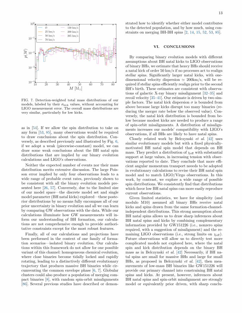
The underlying mass distributions predicted by ourformation models do depend on our assumptions aboutBH natal kicks, as shown concretely in Fig. 7. Thesemodest differences accumulate as BH natal kicks increas-ingly disrupt and deplete all BH-BH binaries. To quantifythe similarity between our distributions, Table I reportsan information-theory-based metric (the KL divergence)that attempts to quantify the information rate or “chan-nel capacity” by which the universe communicates infor-mation about the mass distribution to us. If p(x), q(x) aretwo probability distributions over a parameter x, then ingeneral the KL divergence has the form
DKL(p|q) =
∫dxp(x) ln[p(x)/q(x)] (4)
Except for the strongest BH natal kicks, we find ourmass distributions are nearly identical. Even with perfectmass measurement accuracy, we would need O(1/DKL)

11
0.0 0.2 0.4 0.6 0.8 1.0χ1
0.0
0.2
0.4
0.6
0.8
1.0
χ2
+1.79
+3.87
+3.95
+4.05
+3.75
+3.22
+2.43
+2.53
+1.69
+1.44
+3.37
+4.16
+3.62
+2.95
+6.10
+1.89
+2.61
+2.64
+1.79
+1.05
+3.58
+3.28
+3.97
+4.20
+3.46
+2.38
+2.04
+3.42
+3.38
+2.58
+4.24
+4.33
+2.77
+2.74
+2.78
+2.47
+3.20
+2.93
+1.39
+.546
+3.31
+3.77
+3.96
+4.70
+3.46
+1.35
+2.13
+1.40
+1.79
+1.11
+3.23
+2.59
+3.16
+3.07
+3.31
+2.24
+1.77
-1.38
-.860
+1.89
+5.83
+2.66
+3.87
+2.94
+2.99
+.248
+.985
+1.23
+.329
-.048
+2.04
+5.15
+2.35
+1.77
+2.03
+.849
+1.50
+.721
-.035
+.500
+1.48
+.500
+1.23
+1.25
+1.01
+1.19
+.919
-1.07
-.457
-.281
+.488
+.492
+.085
-.752
+1.98
-1.01
-.627
-.230
-.321
+1.10
−0.8
0.0
0.8
1.6
2.4
3.2
4.0
4.8
5.6
lnK
0.0 0.2 0.4 0.6 0.8 1.0χ1
0.0
0.2
0.4
0.6
0.8
1.0
χ2
+.032
+1.23
+1.93
+1.56
+.677
-.533
+.942
-.108
-1.21
-1.55
+1.98
+2.28
+1.29
+.125
+.060
+1.48
+.208
+.459
-.334
-1.02
+3.28
+3.18
+2.70
+2.35
+1.53
+.806
+.790
-.284
-.669
-1.47
+3.21
+3.03
+3.45
+2.19
+1.11
+1.78
+.892
-.686
+.010
-.962
+3.74
+4.00
+3.80
+3.37
+2.65
+.776
+.158
-1.33
-.997
-1.69
+3.21
+2.74
+3.62
+3.69
+2.56
+2.55
+.982
+.453
-1.22
-1.03
+4.11
+2.37
+2.84
+3.71
+3.17
+3.47
+1.03
+1.20
-.520
-.122
+1.64
+4.55
+2.68
+2.63
+3.14
+3.45
+3.53
+1.73
-.500
+.306
+.525
+1.83
+.303
+2.28
+3.23
+2.12
+2.00
+3.29
+1.14
-.367
+1.01
+.619
+.575
+1.80
+1.91
+2.52
+2.22
+1.98
+2.37
+.709
−1.0
−0.5
0.0
0.5
1.0
1.5
2.0
2.5
3.0
3.5
4.0
lnK
FIG. 5. Bayes factor versus spin, with and without tides (O1): For the M14 model (σ = 200km/s), a plot of the Bayes factorversus χ1,2. Colors and numbers indicate the Bayes factor; dark colors denote particularly unlikely configurations. The leftpanel assumes no spin realignment (“no tides”); the right panel assumes the second-born BH’s progenitor had its spin alignedwith its orbit just prior to birth (“tides”). Spin-orbit realignment and the high orbital velocity just prior to the second SNensures the second spin is at best weakly misaligned; therefore, χ2 would need to be small for these models to be consistentwith LIGO’s observations to date.
fair draws from our distribution to confidently distin-guish between them. As demonstrated by previous stud-ies [79, 83], LIGO will be relatively inefficient at discrimi-nating between the different detected mass distributions.LIGO is most sensitive to the heaviest BHs, which dom-inate the astrophysically observed population, but hasextremely large measurement uncertainty in this regime.Thus, accounting for selection bias and smoothing us-ing estimated measurement error, the mass distributionsconsidered here look fairly similar [79]. For constraintson BH natal kicks, the information provided by the massdistribution is far less informative than the insights im-plied by constraints on χeff and θ1,2.
As a measure of the information LIGO can extractper event about the mass distribution from each de-tection, we enumerate how many different BH-BH bi-naries LIGO can distinguish, which are consistent withthe expected stellar-mass BH-BH population (i.e., moti-vated by LIGO’s reported observations to date, limitingto m2/m1 > 0.5, m1 + m2 < 75M�, m2 > 3M�, andm1 < 40M�). Counting up the distinct waveforms usedby gravitational wave searches in O2 [84], including spin,there are only 236 templates with chirp masses aboveLVT151012 (i.e., Mc > 15M�), and only ' 1,200 withchirp masses above GW151226 (i.e., Mc > 8.88M�).This estimate is highly optimistic, because it neglects dis-tance and hence redshift uncertainty, which decreases ourability to resolve the smallest masses (i.e., the uncertainty
in chirp mass for GW151226), and it also uses both massand spin information. Judging from the reported massdistributions alone (e.g., the top left panel of Fig. 4 in[4]), LIGO may efficiently isolate BHs to only a few tensof distinct mass bins, de facto limiting the resolution ofany mass distribution which can be nonparametricallyresolved with small-number statistics; see, e.g., the dis-cussion in [83].
V. PREDICTIONS AND PROJECTIONS
Using the Bayes factors derived above for our binaryevolution models and BH natal spin assumptions (col-lectively indexed by Λ), we can make predictions aboutfuture LIGO observations, characterized by a probabil-ity distribution pfuture(x) =
∑Λ p(x|Λ)p(Λ|d) for a can-
didate future binary with parameters x. We can thenaccount for LIGO’s mass-dependent sensitivity to gen-erate the relative probability of observing binaries withthose parameters. In the context of the infrastructure de-scribed above, we evaluate this detection-weighted pos-terior probability using a mixture of synthetic universes,with relative probabilities p(Λ|d) and relative weight riof detecting an individual binary drawn from it.
Using our fiducial assumptions about BH spin realign-ment (“no tides”), our posterior probabilities point tononzero BH natal kicks, with BH natal spins that can

12
0.0 0.2 0.4 0.6 0.8 1.0λ
0
2
4
6
dP/dλ
M10
M18
M17
M16
M15
M14
M13
O1+GW170104
O1
−1.0 −0.5 0.0 0.5 1.0χeff
0.0
0.2
0.4
0.6
0.8
1.0
P(<
χeff
)
M10
M18
M17
M16
M15
M14
M13
Tides
No Tides
−1.0 −0.5 0.0 0.5 1.0χeff
0.0
0.2
0.4
0.6
0.8
1.0
P(<
χeff
)
M10
M18
M17
M16
M15
M14
M13
Tides
No Tides
FIG. 6. High or low natal spin? Top panel: Posterior distribution on λA, the fraction of BHs with natal spins ≤ 0.6 [Eq. (3)],based on O1 (dotted) or on O1 with GW170104 (solid), compared with our binary evolution models (colors), assuming “notides.” Unlike Fig. 4, which illustrates Bayes factors calculated assuming fixed BH natal spins, this calculation assumes eachBH natal spin is drawn at random from a mass- and formation-scenario-independent distribution that is piecewise constantabove and below χ = 0.6. With only four observations, LIGO’s observations consistently but weakly favor low BH natal spins.Left panel: Posterior distribution for χeff implied by the distribution of λA shown in the top panel (i.e., by comparing ourmodels to LIGO’s O1 observations, under the assumptions made in Eq. (3)). Right panel: As in the left panel, but includingGW170104. Adding this event does not appreciably or qualitatively change our conclusions relative to O1.
neither be too large nor too small (Figs. 4 and 6). Inturn, because each of our individual formation scenariosΛ preferentially forms binaries with χeff > 0 [55], with astrong preference for the largest χeff allowed, we predictfuture LIGO observations will frequently include binarieswith the largest χeff allowed by the BH natal spin distri-bution. These measurements will self-evidently allow usto constrain the natal spin distribution (e.g., the maxi-mum natal BH spin). For example, if future observationscontinue to prefer small χeff , then the data would increas-
ingly require smaller and smaller natal BH spins, withinthe context of our models. For example, this future sce-nario would let us rule out models with large kicks andlarge spins, as then LIGO should nonetheless frequentlydetect binaries with large χeff .
As previously noted, with only four GW observations,the data does not strongly favor any spin magnitude dis-tribution. Strongly modeled approaches which assumespecific relationships between the relative prior probabil-ity of different natal spins can draw sharper constraints,
13
10 20 30 40 50 60 70 80M [M�]
10−4
10−3
10−2
10−1
100p(M
)Ø
25 km/s
50 km/s
70 km/s
130 km/s
200 km/s
265 km/s
FIG. 7. Detection-weighted total mass distributions of ourmodels, labeled by their σkick values, without accounting forLIGO measurement error. The overall mass distributions arevery similar, particularly for low kicks.
as in [54]. If we allow the spin distribution to take onany form [53, 85], many observations would be requiredto draw conclusions about the spin distribution. Con-versely, as described previously and illustrated by Fig. 6,if we adopt a weak (piecewise-constant) model, we candraw some weak conclusions about the BH natal spindistributions that are implied by our binary evolutioncalculations and LIGO’s observations.
Neither the expected number of events nor their massdistribution merits extensive discussion. The large Pois-son error implied by only four observations leads to awide range of probable event rates, previously shown tobe consistent with all the binary evolution models pre-sented here [26, 57]. Conversely, due to the limited sizeof our model space—the discrete model set and singlemodel parameter (BH natal kicks) explored—these poste-rior distributions by no means fully encompass all of ourprior uncertainty in binary evolution and all we can learnby comparing GW observations with the data. While ourcalculations illuminate how GW measurements will in-form our understanding of BH formation, our calcula-tions are not comprehensive enough to provide authori-tative constraints except for the most robust features.
Finally, all of our calculations and projections havebeen performed in the context of one family of forma-tion scenarios—isolated binary evolution. Our calcula-tions within this framework do not allow for one possiblevariant of this channel: homogeneous chemical evolution,where close binaries become tidally locked and rapidlyrotating, leading to a distinctively different evolutionarytrajectory that produces massive BH binaries while cir-cumventing the common envelope phase [6, 7]. Globularclusters could also produce a population of merging com-pact binaries [8], with random spin-orbit misalignments[86]. Several previous studies have described or demon-
strated how to identify whether either model contributesto the detected population, and by how much, using con-straints on merging BH-BH spins [2, 14, 15, 52, 53, 85].
VI. CONCLUSIONS
By comparing binary evolution models with differentassumptions about BH natal kicks to LIGO observationsof binary BHs, we estimate that heavy BHs should receivea natal kick of order 50 km/s if no processes act to realignstellar spins. Significantly larger natal kicks, with one-dimensional velocity dispersion ' 200km/s, will be re-quired if stellar spins efficiently realign prior to the secondBH’s birth. These estimates are consistent with observa-tions of galactic X-ray binary misalignment [32–35] andrecoil velocity [35–41]. Our estimate is driven by two sim-ple factors. The natal kick dispersion σ is bounded fromabove because large kicks disrupt too many binaries (re-ducing the merger rate below the observed value). Con-versely, the natal kick distribution is bounded from be-low because modest kicks are needed to produce a rangeof spin-orbit misalignments. A distribution of misalign-ments increases our models’ compatibility with LIGO’sobservations, if all BHs are likely to have natal spins.
Closely related work by Belczynski et al. [42] usessimilar evolutionary models but with a fixed physically-motivated BH natal spin model that depends on BHmass. They predict a distribution of χeff with substantialsupport at large values, in increasing tension with obser-vations reported to date. They conclude that more effi-cient angular momentum transport neeeds to be adoptedin evolutionary calculations to revise their BH natal spinmodel and to match LIGO/Virgo observations. In thiswork, by contrast, we explore a wide range of possiblespin distributions. We consistently find that distributionswhich favor low BH natal spins can more easily reproducecurrent observations.
Given limited statistics, we have for simplicity (andmodulo M10) assumed all binary BHs receive natalkicks and spins drawn from the same formation-channel-independent distributions. This strong assumption aboutBH natal spins allows us to draw sharp inferences aboutBH natal spins and kicks by combining complementaryinformation provided by GW151226 (i.e., nonzero spinsrequired, with a suggestion of misalignment) and the re-maining LIGO observations (i.e., strong limits on χeff).Future observations will allow us to directly test morecomplicated models not explored here, where the natalspin and kick distribution depends on the binary BHmass as in Belczynski et al. [42] Necessarily, if BH na-tal spins are small for massive BHs and large for smallBHs, as proposed in Belczynski et al. [42], then mea-surements of low-mass BH binaries like GW151226 willprovide our primary channel into constraining BH natalspins and kicks. At present, however, inferences aboutBH natal spins and spin-orbit misalignment are stronglymodel or equivalently prior driven, with sharp conclu-
14
sions only possible with strong assumptions. We stronglyrecommend results about future BH-BH observations bereported or interpreted using multiple and astrophysi-cally motivated priors, to minimize confusion about theirastrophysical implications (e.g., drawn from the distribu-tion of χeff).
For simplicity, we have also only adjusted one assump-tion (BH natal kicks) in our fiducial model for how com-pact binaries form. A few other pieces of unknown andcurrently parametrized physics, notably the physics ofcommon envelope evolution, should play a substantialrole in how compact binaries form and, potentially, onBH spin misalignment. Other assumptions have muchsmaller impact on the event rate and particularly on BHspin misalignment. Adding additional sources of uncer-tainty will generally diminish the sharpness of our con-clusions. For example, the net event rate depends on theassumed initial mass function as well as the star forma-tion history and metallicity distribution throughout theuniverse; once all systematic uncertainties in these in-puts are inclusded, the relationship between our modelsand the expected number of events is likely to includesignificant systematic as well as statistical uncertainty.Thus, after marginalizing over all sources of uncertainty,the event rate may not be as strongly discriminating be-tween formation scenarios. By employing several inde-pendent observables (rate, masses, spins and misalign-ments), each providing weak constraints about BH natalkicks, we protect our conclusions against systematic er-rors in the event rate. Further investigations are neededto more fully assess sources of systematic error and en-able more precise constraints.
Due to the limited size of our model space—the dis-crete model set and single model parameter (BH na-tal kicks) explored—these posterior distributions by nomeans fully encompass all of our prior uncertainty in bi-nary evolution and all we can learn by comparing GWobservations with the data. As in previous early work[87–90], a fair comparison must broadly explore manymore elements of uncertain physics in binary evolution,like mass transfer and stellar winds. Nonetheless, thisnontrivial example of astrophysical inference shows howwe can learn about astrophysical models via simultane-ously comparing GW measurements of several param-eters of several detected binary BHs to predictions ofany model(s). While we have applied our statistical tech-niques to isolated binary evolution, these tools can beapplied to generic formation scenarios, including homo-geneous chemical evolution; dynamical formation in glob-ular clusters or AGN disks; or even primordial binaryBHs.
Forthcoming high-precision astrometry and radial ve-locity from GAIA will enable higher-precision constraintson existing X-ray binary proper motions and distances[91, 92], as well as increasing the sample size of availableBH binaries. These forthcoming improved constraints onBH binary velocities will provide a complementary av-enue to constrain BH natal kicks using binaries in our
own galaxy.
ACKNOWLEDGMENTS
We thank Christopher Berry, Simon Stevenson, andWill Farr for helpful comments on the draft. D.W.is supported by the Rochester Institute of Technol-ogy (RIT) through the Frontiers in Gravitational WaveAstrophysics (FGWA) Signature Interdisciplinary Re-search Areas (SIRA) initiative and College of Sci-ence. R.O. is supported by NSF Grants No. AST-1412449, PHY-1505629, and PHY-1607520. D.G. is sup-ported by NASA through Einstein Postdoctoral Fel-lowship Grant No. PF6-170152 awarded by the Chan-dra X-ray Center, which is operated by the Smithso-nian Astrophysical Observatory for NASA under Con-tract NAS8-03060. E.B. is supported by NSF GrantsNo. PHY-1607130 and AST-1716715, and by FCT con-tract IF/00797/2014/CP1214/CT0012 under the IF2014Programme. M.K. is supported by the Alfred P. SloanFoundation Grant No. FG-2015-65299 and NSF GrantNo. PHY-1607031. R.O. and E.B. acknowledge the hos-pitality of the Aspen Center for Physics, supported byNSF PHY-1607611, where this work was completed.K.B. acknowledges support from the Polish NationalScience Center (NCN) grant: Sonata Bis 2 (DEC-2012/07/E/ST9/01360). D.E.H. was partially supportedby NSF CAREER grant PHY-1151836 and NSF GrantNo. PHY-1708081. He was also supported by the KavliInstitute for Cosmological Physics at the Universityof Chicago through NSF Grant No. PHY-1125897 andan endowment from the Kavli Foundation. Computa-tions were performed on the Caltech computer cluster“Wheeler,” supported by the Sherman Fairchild Foun-dation and Caltech. Partial support is acknowledgedby NSF CAREER Award PHY-1151197. The authorsthank to the LIGO Scientific Collaboration for access tothe data and gratefully acknowledge the support of theUnited States National Science Foundation (NSF) for theconstruction and operation of the LIGO Laboratory andAdvanced LIGO as well as the Science and TechnologyFacilities Council (STFC) of the United Kingdom, andthe Max-Planck-Society (MPS) for support of the con-struction of Advanced LIGO. Additional support for Ad-vanced LIGO was provided by the Australian ResearchCouncil.
APPENDIX A: APPROXIMATING PARAMETERDISTRIBUTIONS FROM FINITE SAMPLES
Our population synthesis techniques allow us to gen-erate an arbitrarily high number of distinct binary evo-lutions from each formation scenario, henceforth indexedby Λ. Instead of generating individual binary evolutionhistories, we weigh each one by an occurrence rate, al-lowing it to represent multiple binaries. For our calcu-
15
lations, however, we instead require the relative prob-ability of different binaries, not just samples from thedistribution. We estimate this distribution from thelarge but finite sample of binaries available in each syn-thetic universe. We do not simply use an occurrencerate-weighted histogram of all the samples. Histogramswork reliably for any single parameter (e.g., p(m1|Λ)),where many samples are available per potential his-togram bin, but for high-dimensional joint distributions(e.g., p(m1,m2, θ1, θ2, χeff |Λ)), many histogram bins willbe empty simply due to the curse of dimensionality.
In all our calculations, we instead approximate the den-sity as a mixture of Gaussians, labeled k = 1, 2, . . . ,K,with means and covariances (µk, Σk) to be estimated,along with weighting coefficients wk, which must sum tounity. The density can therefore be written as
p(x) ≈K∑k=1
wkN (x|µk,Σk), (A1)
where N (·) represents the (multivariate) Gaussian distri-bution. We select the number of Gaussians K by usingthe Bayesian information criterion.
To estimate the means and covariances of our mixtureof Gaussians, we used the expectation maximization algo-rithm [93]; see, e.g., [94] for a pedagogical introduction.Specifically, we used a small modification to an imple-mentation in scikit-learn [95], to allow for weightedsamples in the update equation (e.g., adding weights toEq. (11.27) in [94]).
Ideally we would simply approximate each formationscenario Λ’s intrinsic predictions p(x|Λ) with a mixtureof Gaussians, using the merger rate for each sample bi-nary as its weighting factor. However, all astrophysicalindications suggest that more massive progenitors formmore rarely, implying this procedure would result in adistribution that is strongly skewed in favor of the muchmore intrinsically frequent low mass systems; our fittingalgorithm might end up effectively neglecting the sampleswith small weights. This would risk losing informationabout the most observationally pertinent samples, whichdue to LIGO’s mass-dependent sensitivity are concen-trated at the highest observationally accessible masses.Alternatively, for every choice of detection network, wecan approximate each formation scenario’s predictionsfor that network. If TV (x) is the average sensitive 4-volume for the network, according to this procedure weapproximate V (x)p(x) by a Gaussian mixture, then di-vide by V (x) to estimate p(x). To minimize duplication ofeffort involved in regenerating our approximation for eachdetector network, we instead adopt a fiducial (approxi-mate) network sensitivity model Vref(x) for the purposesof density estimation. We adopt the simplest (albeit ad-hoc) network sensitivity model: the functional form forV (x) that arises by using a single detector network and
ignoring cosmology (i.e., EV ∝ M15/6c ) [76]. The over-
all, nominally network- and run-dependent normalizationconstant in this ad-hoc model Vref scales out of all final
results.
APPENDIX B: HIERARCHICAL COMPARISONSOF OBSERVATIONS WITH DATA
As described in Sec. III B, the population of binarymergers accessible to our light cone can be described asan inhomogeneous Poisson process, characterized by aprobability density e−µ
∏kRp(xk) where xk = x1 . . . xN
are the distinct binaries in our observationally acces-sible parameter volume V. In this expression, the ex-pected number of events and parameter distribution arerelated by µ =
∫dx√gRp(x); the multidimensional inte-
gral∫dx√g is shorthand for a suitable integration over
a manifold with metric; and the probability density p(x)is expressed relative to the fiducial (metric) volume el-ement, but normalized on a larger volume than V. Ac-counting for data selection [78], the likelihood of all ofour observations is therefore given by Eq. (2).
To insure we fully capture the effects of precess-ing spins, we work not with the full likelihood—a dif-ficult function to approximate in 8 dimensions—butinstead with a fiducial posterior distribution ppost =Z−1p(dk|x)pref(xk), as would be provided by a Bayesiancalculation using a reference prior pref(xk). Rewriting theintegrals
∫dxkp(dk|x)p(xk|Λ) appearing in Eq. (2) using
the reference prior we find integrals appearing in this ex-pression can be calculated by Monte Carlo, using somesampling distribution ps,k(xk) for each event (see, e.g.,[96]):∫
dxkp(dk|xk)p(xk|Λ)
=1
Nk
∑s
[p(dk|xk)pref(xk,s)]p(xk,s|Λ)
ps,k(xk,s)pref(xk,s), (B1)
where s = 1, . . . Nk indexes the Monte Carlo samplesused. One way to evaluate this integral is to adopt a sam-pling distribution ps,k equal to the posterior distributionevaluated using the reference prior, and thus proportionalto p(dk|xk)pref(xk|Λ). If for this event k we have samplesxk,s from the posterior distribution—for example, as pro-vided by a Bayesian Markov chain Monte Carlo code—the integrals appearing in Eq. (2) can be estimated by∫
dxkp(dk|xk)p(xk|Λ) ' Z
Nk
∑s
p(xk,s|Λ)
pref(xk,s), (B2)
We use this expression to evaluate the necessary marginallikelihoods, for any proposed observed population p(x|Λ).
In the expression above, we need only consider someof the degrees of freedom in the problem. Notably, theprobability distributions for extrinsic parameters like thesource orientation, sky location, and distance will al-ways be in common between our models and our refer-ence prior. So will any Jacobians associated with changes

16
of coordinate. Moreover, these assumptions are indepen-dent of one another and of the intrinsic parameter dis-tributions. Therefore, the ratio of probability densitiesp(x|Λ)/pref(x) usually has product form, canceling termby term. We therefore truncate the ratio to only accountfor some of the degrees of freedom.
To verify and better understand our results, we canalso approximate the likelihood function, using suitablesummary statistics. As an example, Abbott, B. P. et al.(LIGO and Virgo Scientific Collaboration) [49] reproduceparameter estimates of GW150914 using a Gaussian ap-proximation to the likelihood and the assumption of per-fect spin-orbit alignment. Using this approximation, anda similar approximation for GW151226, we can alterna-tively approximate each integral appearing in the likeli-hood by using the (weighted) binary evolution samplesxk,A and their weights wA:
∫dxkp(dk|xk)p(xk|Λ) '
∑A wAp(dk|xk,A)∑
A wA(B3)
where p refers to our approximate likelihood for the kthevent. Even though these likelihood approximations ne-glect degrees of freedom associated with spin precession,we can reproduce the observed mass and χeff distribu-tions reported in Abbott, B. P. et al. (LIGO and VirgoScientific Collaboration) [49]. We used this approximatelikelihood approach to validate and test our procedure.We also use this approach to incorporate informationabout GW170104, which was not available at the samelevel of detail as the other events.
As an example, we describe how to evaluate this in-tegral in the case where p(xk|λ) is a mixture modelp(x|λ) =
∑α λαpα(x), for λ an array of parameters. In
this case, all the integrals can be carried out via∏k
∫dxkp(dk|xk)p(xk|λ) (B4)
=∏k
[∑α
λα
∫dxkp(dk|xk)pα(xk)] =
∏k
∑α
λαcα,k
where cα,k are integrals we can compute once and for allfor each event, using for example the posterior samplesfrom some fiducial analysis. As a result, the observation-dependent factor in likelihood for a mixture model alwaysreduces to a homogeneous Nth-degree polynomial in themixture parameters λα. Bayes theorem can be appliedto λ to infer the distribution over mixture parameters.Depending on the mixture used, this calculation couldincorporate a physically-motivated prior on λ.
We use a mixture model approach to hierarchicallyconstrain the spin magnitude distribution implied by ourdata. In our approach, we first consider models whereboth spin magnitudes are fully constrained. In the no-tation of the mixture model discussion above, we adoptsome specific prior pα(χ1, χ2|σ) = δ(χ1 − xα)δ(χ2 − yα)where xα, yα are the spin λα. A mixture model allow-ing generic λ and thus including all such componentsallows both component spins to take arbitrary (discrete)values. [We could similarly extend our mixture model toinclude kicks.] The posterior distribution over all possiblespin distributions p(λ|d) = p(d|λ)p(λ)/p(d) follows fromBayes’ theorem and the concrete likelihood given in Eq.(B4). In practice, however, we don’t generally computeor report the full posterior distribution, as it contains farmore information than we need (e.g., the extent of theensemble of possible spin distributions that fit the data).Instead, we compute the expected spin distribution
ppost(x) =∑α
〈λα〉pα(x) (B5)
and the variance in each λα. For the modest numberof mixture components of interest here (' 100 possiblechoices of both spin magnitudes) and the modest degreeof the polynomial (' 4 − 5), all necessary averages canbe computed by direct symbolic quadrature of a polyno-mial in λα. The integral can be expressed as a sum ofterms of homogeneous degree in λ, and integrals of eachof these terms can be carried out via the following generalformula:
n!
∫∑
i xi≤1
dx1 . . . dxnxα1i1. . . xαZ
iZ=
n!
(n− Z)!
Z∏k=1
B(αk + 1, n+ 1− k +∑q>k
αq) (B6)
where the integral is over the region xi ≥ 0 and∑i xi ≤
1. We can also find the maximum likelihood estimate ofλα, for example by using the expectation-maximization
algorithm [93]. In this work, however, we have many morebasis models α = 1, 2, . . . used in our (spin) mixturethan observations. Normally, we would reduce the effec-
17
tive dimension, for example by adopting prior assump-tions in how the mixture coefficients can change as afunction of spins χ1, χ2. To minimize additional formaloverhead, we instead simply treat the spins hierarchicallyin blocks [Eq. (3)], considering lower-dimensional mod-els where (for example) λA denotes the a priori prob-ability for χi ≤ 0.6 and 1 − λA denotes the a prioriprobability for χi > 0.6, so for example the prior prob-ability for (χ1, χ2) = 0.1 is λ2
A/36. In this four-blockand one-parameter model, we can compute the averagevalue of λA in terms of the net weights associated witheach block: CAA,k =
∑χ1,χ2∈A cα,k, CAAk, CAAk and
CAAk. For example, if for each of three synthetic obser-vations, CAA = 1 and all other weights are negligible,then we would conclude a posterori that 〈λA〉 = 0.875and σλA
= 0.11. This approach was adopted in Fig. 6,in contrast to the preceding figures which adopted fixednatal spins for all BHs.
APPENDIX C: APPROXIMATE POSTERIORDISTRIBUTION FOR GW170104
For most events examined in this study, we made use ofposterior samples provided and performed by the LIGOScientific Collaboration, generated by comparing eachevent to the IMRPv2 approximation [72]. Because wecannot employ the same level of detail for GW170104,we instead resort to an approximate posterior distribu-tion, derived from the reported GW170104 results [5] andour understanding of gravitational wave parameter esti-mation, as approximated using a Fisher matrix [97].
For GW170104 we construct an approximate (trun-cated) Gaussian posterior distribution in only three cor-related binary parameters:Mc, η, χeff . The shape of thisGaussian (i.e., its inverse covariance matrix) was con-
structed via a Fisher matrix approximation, derived us-ing the median detector-frame parameters reported forGW170104 (i.e., m1 ' 37.1M�, m2 ' 22.6M�, and—breaking degeneracy with an ad-hoc choice—χ1,zχ2,z 'χeff ' −0.12); the reported network SNR of GW170104(i.e., ρ ' 13.0); and a suitable single-detector noisepower spectrum. Our effective Fisher matrix estimatefor the inverse covariance matrix Γ [98] adopted thenoise power spectrum at GW150914, using a minimumfrequency fmin = 30Hz; employed the (nonprecessing)SEOBNRv4 approximation [99], evaluated on a gridin Mc, η, χ1,z, χ2,z; and fit as a quadratic function ofMc, η, χeff . We adopt a nonprecessing model and lower-dimensional Fisher matrix approximation because theposterior of this event, like GW150914, is consistent withnonprecessing spins and is very well approximated, inthese parameters, by a nonprecessing model; see, e.g.,[49]. This simple approximation captures important cor-relations betweenMc, η and χeff , and the diagonal termsof Γ−1ρ2 roughly reproduce the width of the posteriordistribution reported for GW170104. To obtain betteragreement with the reported one-dimensional credible in-tervals, we scaled the terms ΓMc,x for x = Mc, η, χeff
by a common scale factor 0.29 and the term Γχeff ,χeff
by 0.9. For similar reasons, we likewise hand-tuned thecenter of the Gaussian distribution to the (unphysical)parameter location toMc = 22.9, η = 0.32, χeff = 0.013.Using this ansatz, we generate GW170104-like posteriorsamples in Mc, η, χeff from this Gaussian distribution,truncating any unphysical samples (i.e., with η > 1/4).For our tuned posterior, the median and 90% credibleregions on the synthetic posteriors approximate the val-ues and ranges reported. According to our highly sim-plified and purely synthetic approach, the resulting 90%credible regions are Mtot = 51.2+7.6
−6.8M�, q = 0.62+0.25−0.24,
χeff = −0.12+0.28−0.27.
[1] Abbott, B. P. et al. (LIGO and Virgo Scientific Collabo-ration), PRL 116, 061102 (2016).
[2] Abbott, B. P. et al. (LIGO and Virgo Scientific Collabo-ration), ApJ 818, L22 (2016).
[3] Abbott, B. P. et al. (LIGO and Virgo Scientific Collabo-ration), ApJ 833, L1 (2016).
[4] Abbott, B. P. et al. (LIGO and Virgo Scientific Collabo-ration), PRX 6, 041015 (2016).
[5] Abbott, B. P. et al. (LIGO and Virgo Scientific Collabo-ration), PRL 118, 221101 (2017).
[6] I. Mandel and S. E. de Mink, MNRAS 458, 2634 (2016).[7] P. Marchant, N. Langer, P. Podsiadlowski, T. M. Tauris,
and T. J. Moriya, A&A 588, A50 (2016).[8] C. L. Rodriguez, C.-J. Haster, S. Chatterjee, V. Kalogera,
and F. A. Rasio, ApJ 824, L8 (2016).[9] S. Bird, I. Cholis, J. B. Munoz, Y. Ali-Haımoud,
M. Kamionkowski, E. D. Kovetz, A. Raccanelli, andA. G. Riess, PRL 116, 201301 (2016).
[10] D. Kushnir, M. Zaldarriaga, J. A. Kollmeier, andR. Waldman, MNRAS 462, 844 (2016).
[11] A. Lamberts, S. Garrison-Kimmel, D. R. Clausen, andP. F. Hopkins, MNRAS 463, L31 (2016).
[12] I. Dvorkin, E. Vangioni, J. Silk, J.-P. Uzan, and K. A.Olive, MNRAS 461, 3877 (2016).
[13] Abbott, B. P. et al. (LIGO and Virgo Scientific Collabo-ration), PRL 116, 131102 (2016).
[14] C. L. Rodriguez, M. Zevin, C. Pankow, V. Kalogera, andF. A. Rasio, ApJ 832, L2 (2016).
[15] R. O’Shaughnessy, D. Gerosa, and D. Wysocki, PRL119, 011101 (2017).
[16] K. Breivik, C. L. Rodriguez, S. L. Larson, V. Kalogera,and F. A. Rasio, ApJ 830, L18 (2016).
[17] A. Nishizawa, E. Berti, A. Klein, and A. Sesana, PRD94, 064020 (2016).
[18] A. V. Tutukov and L. R. Yungelson, MNRAS 260, 675(1993).
[19] V. M. Lipunov, K. A. Postnov, and M. E. Prokhorov,MNRAS 288, 245 (1997).
[20] K. Belczynski, V. Kalogera, and T. Bulik, ApJ 572, 407(2002).
18
[21] G. Nelemans, L. R. Yungelson, and S. F. PortegiesZwart, A&A 375, 890 (2001).
[22] R. Voss and T. M. Tauris, MNRAS 342, 1169 (2003).[23] M. Dominik, K. Belczynski, C. Fryer, D. E. Holz,
E. Berti, T. Bulik, I. Mandel, and R. O’Shaughnessy,ApJ 759, 52 (2012).
[24] M. Dominik, K. Belczynski, C. Fryer, D. E. Holz,E. Berti, T. Bulik, I. Mandel, and R. O’Shaughnessy,ApJ 779, 72 (2013).
[25] M. Dominik, E. Berti, R. O’Shaughnessy, I. Mandel,K. Belczynski, C. Fryer, D. E. Holz, T. Bulik, andF. Pannarale, ApJ 806, 263 (2015).
[26] K. Belczynski, D. E. Holz, T. Bulik, andR. O’Shaughnessy, Nature 534, 512 (2016).
[27] J. J. Eldridge and E. R. Stanway, MNRAS 462, 3302(2016).
[28] S. Stevenson, A. Vigna-Gomez, I. Mandel, J. W. Barrett,C. J. Neijssel, D. Perkins, and S. E. de Mink, NatureCommunications 8, 14906 (2017).
[29] G. Hobbs, D. R. Lorimer, A. G. Lyne, and M. Kramer,MNRAS 360, 974 (2005).
[30] D. Gerosa, M. Kesden, E. Berti, R. O’Shaughnessy, andU. Sperhake, PRD 87, 104028 (2013).
[31] V. Kalogera, ApJ 541, 319 (2000).[32] R. M. Hjellming and M. P. Rupen, Nature 375, 464
(1995).[33] J. A. Orosz and C. D. Bailyn, ApJ 477, 876 (1997).[34] J. A. Orosz, E. Kuulkers, M. van der Klis, J. E. McClin-
tock, M. R. Garcia, P. J. Callanan, C. D. Bailyn, R. K.Jain, and R. A. Remillard, ApJ 555, 489 (2001).
[35] R. G. Martin, C. A. Tout, and J. E. Pringle, MNRAS401, 1514 (2010).
[36] S. Repetto, M. B. Davies, and S. Sigurdsson, MNRAS425, 2799 (2012).
[37] S. Repetto and G. Nelemans, MNRAS 453, 3341 (2015).[38] S. Repetto, A. P. Igoshev, and G. Nelemans, MNRAS
467, 298 (2017).[39] K. Belczynski, S. Repetto, D. E. Holz, R. O’Shaughnessy,
T. Bulik, E. Berti, C. Fryer, and M. Dominik, ApJ 819,108 (2016).
[40] T.-W. Wong, F. Valsecchi, T. Fragos, and V. Kalogera,ApJ 747, 111 (2012).
[41] T.-W. Wong, F. Valsecchi, A. Ansari, T. Fragos,E. Glebbeek, V. Kalogera, and J. McClintock, ApJ 790,119 (2014).
[42] K. Belczynski, J. Klencki, G. Meynet, C. L. Fryer, D. A.Brown, M. Chruslinska, W. Gladysz, R. O’Shaughnessy,T. Bulik, E. Berti, D. E. Holz, D. Gerosa, M. Giersz,S. Ekstrom, C. Georgy, A. Askar, J.-P. Lasota, andD. Wysocki, (2017), arXiv:1706.07053.
[43] K. Belczynski and T. Bulik, A&A 346, 91 (1999).
[44] E. Racine, PRD 78, 044021 (2008).[45] M. Kesden, D. Gerosa, R. O’Shaughnessy, E. Berti, and
U. Sperhake, PRL 114, 081103 (2015).[46] D. Gerosa, M. Kesden, U. Sperhake, E. Berti, and
R. O’Shaughnessy, PRD 92, 064016 (2015).[47] J. Veitch, V. Raymond, B. Farr, W. Farr, P. Graff,
S. Vitale, B. Aylott, K. Blackburn, N. Christensen,M. Coughlin, W. Del Pozzo, F. Feroz, J. Gair, C.-J. Haster, V. Kalogera, T. Littenberg, I. Mandel,R. O’Shaughnessy, M. Pitkin, C. Rodriguez, C. Rover,T. Sidery, R. Smith, M. Van Der Sluys, A. Vecchio,W. Vousden, and L. Wade, PRD 91, 042003 (2015).
[48] Abbott, B. P. et al. (LIGO and Virgo Scientific Collabo-ration), PRL 116, 241102 (2016).
[49] Abbott, B. P. et al. (LIGO and Virgo Scientific Collabo-ration), PRD 94, 064035 (2016).
[50] D. Trifiro, R. O’Shaughnessy, D. Gerosa, E. Berti,M. Kesden, T. Littenberg, and U. Sperhake, PRD 93,044071 (2016).
[51] D. Gerosa, R. O’Shaughnessy, M. Kesden, E. Berti, andU. Sperhake, PRD 89, 124025 (2014).
[52] S. Vitale, R. Lynch, R. Sturani, and P. Graff, CQG 34,03LT01 (2017).
[53] S. Stevenson, C. P. L. Berry, and I. Mandel, MNRAS471, 2801 (2017).
[54] W. M. Farr, S. Stevenson, M. C. Miller, I. Mandel,B. Farr, and A. Vecchio, Nature 548, 426 (2017).
[55] D. Gerosa, R. O’Shaughnessy, K. Belczynski,W. Gladerys, D. Wysocki, E. Berti, M. Kesden,et al., In preparation (2017).
[56] See Supplemental Material at http://link.aps.org/
supplemental/10.1103/PhysRevD.97.043014, whichcontains ASCII tables providing the means, rates andintegrals in Equation (2), which may be used to repro-duce many of our analyses, and explore combinations ofmodels not investigated in this paper.
[57] K. Belczynski, A. Heger, W. Gladysz, A. J. Ruiter,S. Woosley, G. Wiktorowicz, H.-Y. Chen, T. Bulik,R. O’Shaughnessy, D. E. Holz, C. L. Fryer, and E. Berti,A&A 594, A97 (2016).
[58] K. Belczynski, V. Kalogera, F. A. Rasio, R. E. Taam,A. Zezas, T. Bulik, T. J. Maccarone, and N. Ivanova,ApJS 174, 223-260 (2008).
[59] C. L. Fryer, K. Belczynski, G. Wiktorowicz, M. Dominik,V. Kalogera, and D. E. Holz, ApJ 749, 91 (2012).
[60] G. E. Brown, C.-H. Lee, R. A. M. J. Wijers, H. K. Lee,G. Israelian, and H. A. Bethe, New A 5, 191 (2000).
[61] J. M. Bardeen, Nature 226, 64 (1970).[62] K. S. Thorne, ApJ 191, 507 (1974).[63] R. O’Shaughnessy, J. Kaplan, V. Kalogera, and K. Bel-
czynski, ApJ 632, 1035 (2005).[64] P. Hut, A&A 99, 126 (1981).[65] T. Mazeh, in EAS Publications Series, EAS Publications
Series, Vol. 29, edited by M.-J. Goupil and J.-P. Zahn(2008) pp. 1–65.
[66] S. Albrecht, J. Setiawan, G. Torres, D. C. Fabrycky, andJ. N. Winn, ApJ 767, 32 (2013).
[67] K. Belczynski, R. E. Taam, V. Kalogera, F. A. Rasio,and T. Bulik, ApJ 662, 504 (2007).
[68] K. Belczynski, R. E. Taam, E. Rantsiou, and M. van derSluys, ApJ 682, 474-486 (2008).
[69] A. R. King and U. Kolb, MNRAS 305, 654 (1999).[70] P. Natarajan and J. E. Pringle, ApJ 506, L97 (1998).[71] D. Gerosa and M. Kesden, PRD 93, 124066 (2016).[72] M. Hannam, P. Schmidt, A. Bohe, L. Haegel, S. Husa,
F. Ohme, G. Pratten, and M. Purrer, PRL 113, 151101(2014).
[73] A. Taracchini, A. Buonanno, Y. Pan, T. Hinderer,M. Boyle, D. A. Hemberger, L. E. Kidder, G. Lovelace,A. H. Mroue, H. P. Pfeiffer, M. A. Scheel, B. Szilagyi,N. W. Taylor, and A. Zenginoglu, PRD 89, 061502(2014).
[74] J. Blackman, S. E. Field, M. A. Scheel, C. R. Galley,C. D. Ott, M. Boyle, L. E. Kidder, H. P. Pfeiffer, andB. Szilagyi, PRD 96, 024058 (2017).
[75] J. Blackman, S. E. Field, M. A. Scheel, C. R. Galley,

19
D. A. Hemberger, P. Schmidt, and R. Smith, PRD 95,104023 (2017).
[76] R. O’Shaughnessy, V. Kalogera, and K. Belczynski, ApJ716, 615 (2010).
[77] Abbott, B. P. et al. (LIGO and Virgo Scientific Collabo-ration), PRL 116, 241103 (2016).
[78] T. J. Loredo, in American Institute of Physics ConferenceSeries, American Institute of Physics Conference Series,Vol. 735, edited by R. Fischer, R. Preuss, and U. V.Toussaint (2004) pp. 195–206.
[79] S. Stevenson, F. Ohme, and S. Fairhurst, ApJ 810, 58(2015).
[80] R. O’Shaughnessy, PRD 88, 084061 (2013).[81] S. Vitale, D. Gerosa, C.-J. Haster, K. Chatziioan-
nou, and A. Zimmerman, Physical Review Letters 119,251103 (2017).
[82] A. R. Williamson, J. Lange, R. O’Shaughnessy, J. A.Clark, P. Kumar, J. Calderon Bustillo, and J. Veitch,PRD 96, 124041 (2017).
[83] M. Zevin, C. Pankow, C. L. Rodriguez, L. Sampson,E. Chase, V. Kalogera, and F. A. Rasio, ApJ 846, 82(2017).
[84] C. Capano, I. Harry, S. Privitera, and A. Buonanno,PRD 93, 124007 (2016).
[85] C. Talbot and E. Thrane, PRD 96, 023012 (2017).[86] R. O’Shaughnessy, Presentation at Syracuse University
(2009).[87] R. O’Shaughnessy, C. Kim, T. Fragos, V. Kalogera, and
K. Belczynski, ApJ 633, 1076 (2005).[88] R. O’Shaughnessy, C. Kim, V. Kalogera, and K. Bel-
czynski, ApJ 672, 479-488 (2008).[89] R. O’Shaughnessy, K. Belczynski, and V. Kalogera, ApJ
675, 566-585 (2008).[90] I. Mandel and R. O’Shaughnessy, CQG 27, 114007
(2010).[91] Gaia Collaboration, T. Prusti, J. H. J. de Bruijne,
A. G. A. Brown, A. Vallenari, C. Babusiaux, C. A. L.Bailer-Jones, U. Bastian, M. Biermann, D. W. Evans,and et al., A&A 595, A1 (2016).
[92] Gaia Collaboration, A. G. A. Brown, A. Vallenari,T. Prusti, J. H. J. de Bruijne, F. Mignard, R. Drimmel,C. Babusiaux, C. A. L. Bailer-Jones, U. Bastian, andet al., A&A 595, A2 (2016).
[93] A. Dempster, N. Laird, and D. Rubin, Journal of theRoyal Statistical Society. Series B (Methodological) 39,1 (1977).
[94] K. P. Murphy, “Machine learning: a probabilistic per-spective,” (2012).
[95] F. Pedregosa, G. Varoquaux, A. Gramfort, V. Michel,B. Thirion, O. Grisel, M. Blondel, P. Prettenhofer,R. Weiss, V. Dubourg, J. Vanderplas, A. Passos, D. Cour-napeau, M. Brucher, M. Perrot, and E. Duchesnay, Jour-nal of Machine Learning Research 12, 2825 (2011).
[96] D. W. Hogg, A. D. Myers, and J. Bovy, ApJ 725, 2166(2010).
[97] C. Cutler and E. E. Flanagan, PRD 49, 2658 (1994).[98] H.-S. Cho, E. Ochsner, R. O’Shaughnessy, C. Kim, and
C.-H. Lee, PRD 87, 024004 (2013).[99] A. Bohe, L. Shao, A. Taracchini, A. Buonanno, S. Babak,
I. W. Harry, I. Hinder, S. Ossokine, M. Purrer, V. Ray-mond, T. Chu, H. Fong, P. Kumar, H. P. Pfeiffer,M. Boyle, D. A. Hemberger, L. E. Kidder, G. Lovelace,M. A. Scheel, and B. Szilagyi, PRD 95, 044028 (2017).