explicitly staged software pipelining
TRANSCRIPT

Explicitly Staged Software Pipelining


Explicitly Staged Software Pipelining
ByWolfgang Thaller
A ThesisSubmitted to the School of Graduate Studies
in Partial Fulfillment of the Requirementsfor the Degree
Master of Science
McMaster Universityc© Wolfgang Thaller, August 2006

MASTER OF SCIENCE(2006) McMaster UniversityCOMPUTING AND SOFTWARE Hamilton, Ontario
TITLE: Explicitly Staged Software Pipelining
AUTHOR: Wolfgang Thaller
SUPERVISORS: Dr. Christopher Kumar Anand and Dr. Wolfram Kahl
NUMBER OF PAGES: xi, 59
ii

Abstract
Software Pipelining is a method of instruction scheduling where loopsare scheduled more efficiently by executing operations from more than oneiteration of the loop in parallel. Finding an optimal software pipelined scheduleis NP-complete, but many heuristic algorithms exist.
In iteration i , a software pipelined loop will execute, in parallel, ”stage”1 of iteration i , stage 2 of iteration i − 1 and so on until stage k of iterationi − k + 1.
We present a new approach to software pipelining based on using aheuristic algorithm to explicitly assign each operation to its stage before theactual scheduling.
This explicit assignment allows us to implement control flow mecha-nisms that are hard to implement with traditional methods of software pipelin-ing, which do not give us direct control over what stages instructions are as-signed to.
iii

iv

Acknowledgements
My sincere thanks go to my supervisors, Dr. Christopher Anand andDr. Wolfram Kahl, for all the support and guidance they provided. Additionalthanks go to Dr. Anand for a great canoeing and camping trip that helpedme recover from thesis-induced exhaustion.
I would also like to thank my family and friends in Austria for support-ing me from afar, and finally my friends here in Canada for making me feel athome here.
v

vi

Contents
Abstract iii
Acknowledgements v
List of Figures ix
List of Tables xi
1 Introduction 1
1.1 Software Pipelining . . . . . . . . . . . . . . . . . . . . . . . . 3
1.1.1 Kernel-based Methods . . . . . . . . . . . . . . . . . . 4
1.1.2 Modulo Scheduling . . . . . . . . . . . . . . . . . . . . 4
1.1.3 Decomposed Software Pipelining . . . . . . . . . . . . 4
1.1.4 Register Issues . . . . . . . . . . . . . . . . . . . . . . 4
1.2 The Cell Synergistic Processor Unit . . . . . . . . . . . . . . . 5
2 Representation 7
2.1 Codegraphs . . . . . . . . . . . . . . . . . . . . . . . . . . . . 7
2.2 Loop Specifications . . . . . . . . . . . . . . . . . . . . . . . . 10
2.3 Maximum Lifetime and Loopability . . . . . . . . . . . . . . . 11
2.4 Loop Termination . . . . . . . . . . . . . . . . . . . . . . . . . 13
2.5 Example . . . . . . . . . . . . . . . . . . . . . . . . . . . . . . 13
3 Theory of Staging 17
3.1 Pipelining Transformation . . . . . . . . . . . . . . . . . . . . 19
3.2 Prologue and Epilogue . . . . . . . . . . . . . . . . . . . . . . 23
3.3 Loop Termination Revisited . . . . . . . . . . . . . . . . . . . 25
3.4 Correctness . . . . . . . . . . . . . . . . . . . . . . . . . . . . 26
3.5 Example . . . . . . . . . . . . . . . . . . . . . . . . . . . . . . 26
vii

4 Heuristic Staging 294.1 Height and Depth . . . . . . . . . . . . . . . . . . . . . . . . . 304.2 Stage Constraints . . . . . . . . . . . . . . . . . . . . . . . . . 324.3 Stage Separation . . . . . . . . . . . . . . . . . . . . . . . . . 34
5 Merge Scheduling 375.1 Separate Scheduling . . . . . . . . . . . . . . . . . . . . . . . . 375.2 Merging . . . . . . . . . . . . . . . . . . . . . . . . . . . . . . 40
5.2.1 Merging without dependences . . . . . . . . . . . . . . 415.2.2 Merging with antidependences only . . . . . . . . . . . 425.2.3 Handling forward dependences . . . . . . . . . . . . . . 43
6 Adding Control Flow — The Multiloop 45
7 Experimental Results 497.1 Simple Loops . . . . . . . . . . . . . . . . . . . . . . . . . . . 497.2 Multiloop . . . . . . . . . . . . . . . . . . . . . . . . . . . . . 54
8 Conclusions & Outlook 59
viii

List of Figures
2.1 Simple codegraphs . . . . . . . . . . . . . . . . . . . . . . . . 82.2 Loop that squares all elements in an array . . . . . . . . . . . 142.3 Improved Loop for Software Pipelining . . . . . . . . . . . . . 16
3.1 Software pipelining with three stages . . . . . . . . . . . . . . 183.2 Inter-iteration dependences in a pipelined loop . . . . . . . . . 193.3 Splitting a codegraph into three stages . . . . . . . . . . . . . 213.4 Putting the stages together in parallel . . . . . . . . . . . . . . 223.5 Prologue of loop with three stages . . . . . . . . . . . . . . . . 243.6 Prologue of loop with three stages . . . . . . . . . . . . . . . . 273.7 Pipelined loop, with three stages . . . . . . . . . . . . . . . . 28
4.1 Transforming parts of a codegraph to a minimum cut problem 35
5.1 Avoiding dependence cycles when scheduling seperately . . . . 39
ix

x

List of Tables
7.1 Results of scheduling math functions in simple loops for un-rolling factors 1 (no unrolling) and 2 . . . . . . . . . . . . . . 50
7.2 Results of scheduling math functions in simple loops for un-rolling factors 3 and 4 . . . . . . . . . . . . . . . . . . . . . . 51
7.3 Merge Scheduling vs. List Scheduling, unrolling factors 1 and 2 527.4 Merge Scheduling vs. List Scheduling, unrolling factors 3 and 4 537.5 Scheduling results for the 3D resampling multiloop, cases 0
through 26 . . . . . . . . . . . . . . . . . . . . . . . . . . . . . 567.6 Scheduling results for the 3D resampling multiloop, cases 27
through 53 . . . . . . . . . . . . . . . . . . . . . . . . . . . . . 57
xi

M.Sc. Thesis – W. Thaller – McMaster – Computing and Software
xii

Chapter 1
Introduction
With the advent of pipelined execution, instruction scheduling was born; twoinstructions that do not depend on each other can be executed in parallel, whiledependences between instructions can force the processor to finish executingone instruction before starting to execute another. Among the many possibleorderings of instructions that produce the same result, the goal is to find onethat minimises (or comes close to minimising) the number of machine cyclesrequired to execute the code.
Given a piece of straight-line code, that is code without any branches,there are two obvious lower bounds to the number of cycles required for anoptimal schedule. One of them stems from the limited availability of CPUresources — the CPU can only execute a limited number of instructions at thesame time.
The other lower bound is the sum of instruction latencies through thelongest path in the data dependency graph.
In a loop, we can sometimes do better than just to rearrange the in-structions within the loop body with respect to each other. If we can reach theresource-constrained lower bound, there is nothing we can do to improve theschedule any more, except, of course, for improvements in instruction selectionor in the algorithm that is used, which falls outside the scope of this thesis.
If, however, our schedule is latency-constrained, there are some tricksthat can be used to improve matters. The best known of these is loop un-rolling or replication, where the loop body is replicated n times, such thatone loop iteration in the final schedule does the work of n consecutive “logicaliterations” in the original code. In addition to making the cost of the branchsmaller in relation to the cost of the loop body, this frees up some opportunitiesto overlap instructions from different logical iterations.
However, replication is not actually necessary to allow overlapping of in-
1

M.Sc. Thesis – W. Thaller – McMaster – Computing and Software
structions from different logical iterations. Consider a loop with two operationsthat depend on each other, such as (AB)n ; this is equivalent to A(BA)n−1B ,with one important difference: in the transformed loop, the operations A andB operate on data from two different logical iterations and therefore may nolonger depend on each other.
This work was developed as part of the Coconut project, which pre-pares to produce a system that provides a coherent and consistent path from amathematical specification of signal processing problems to verified and highlyoptimised machine code [ACK+04]. One of the hypotheses of this project isthat more efficient implementations would be possible if the interface betweenthe compiler front and back-ends were more flexible and extensible.
In this thesis, we present a new software pipelining scheduling methodrelated to decomposed software pipelining (section 1.1.3). It consists of aheuristic algorithm to assign operations to different pipeline “stages” (chap-ter 4) and an accurate description of how a non-pipelined loop can be trans-formed to a pipelined loop once the staging is known (chapter 3).
In line with the idea of exposing flexible interfaces from the compilerbackend, the representation of the input for the scheduler (chapter 2) allowsus to specify inter-iteration dataflow in loops explicitly, even if that causes theloop to become unschedulable without software pipelining — in a software-pipelined loop, it is sometimes possible to use a value that is produced in afuture iteration (see sections 2.5 and 3.5 for an example of this).
Taking advantage of our scheduling algorithm’s properties, we intro-duce a limited form of control flow that can be scheduled especially well usingour algorithm; a multiloop (chapter 6) is a loop that consists of a block ofcommon code followed by a “switch” or “case” construct with an arbitrarynumber of different cases.
In chapter 5, we explore “Merge Scheduling”, a novel approach toscheduling the output of our stage assignment heuristic, based on the ideaof scheduling the stages separately and then “merging” them into one using adynamic programming algorithm.
Finallly, we give experimental results for our algorithms for our targetarchitecture of choice, the Cell Synergistic Processor Unit (see section 1.2 and[IBM06]).
The remainder of this chapter will give a very brief survey of otherapproaches to software pipelining and to the relevant aspects of the Cell ar-chitecture.
2

M.Sc. Thesis – W. Thaller – McMaster – Computing and Software
1.1 Software Pipelining
Software Pipelining [AJLA95] is the problem of finding a schedule for a loopwhile honoring both dependence and resource constraints, but without requir-ing that one iteration of the loop is finished before the next iteration starts.
The loop contains a set of operations opi which are executed once ineach iteration; we refer to the instance of operation opi in iteration j as (opi , j ).
Resource constraints restrict which operations can be scheduled in thesame cycle. Dependence constraints restrict the relative ordering of the op-erations and also may require a certain number of cycles (latency) to passbetween two instructions.
There are three kinds of dependence constraints:
data dependence (read after write) Operation A calculates a value; op-eration B uses this value, so B has to be scheduled after A. Most instruc-tions on most architectures take more than one machine cycle until thedata is actually available (latency).
antidependence (write after read) Operation A uses a value that will beoverwritten by operation B, so operation A has to be scheduled beforeoperation B.
output dependence (write after write) Both operations A and B storetheir result in the same location, so the order of execution matters.
Dependences between two operations in the same iteration are calledloop independent ; dependences between different iterations of the loop arecalled loop carried.
In the data dependency graph, each node represents an operation opi .Different instances (opi , j ) and (opi , j ) of that operation are represented bythe same node. Edges in the dependency graph are labelled with the requiredlatency (for data dependences) and with the difference in iterations (0 for loopindependent dependences).
Let us consider the schedule for a completely unrolled loop; in conven-tional scheduling, all operations of iteration j will have been issued before thefirst operation of iteration j + 1 is issued. In a software-pipelined loop, this isnot the case; iteration j + 1 will be initiated before iteration j completes.
We require the unrolled schedule to reach a repeating pattern after ashort while (otherwise, the result would be code bloat proportional to the num-ber of iterations). The number of cycles between the start of two consecutive(but overlapping) iterations is termed the initiation interval, or λ.
3

M.Sc. Thesis – W. Thaller – McMaster – Computing and Software
1.1.1 Kernel-based Methods
One approach to software pipelines is to completely unroll the loop, run aconventional scheduling algorithm on it and wait for a repeating pattern toemerge. The drawbacks to this approach are that a repeating pattern mightnot emerge under all circumstances, and that the resulting kernel might belonger than desired, i.e. contain multiple copies of each operation.
1.1.2 Modulo Scheduling
In modulo scheduling [RG81], the λ is chosen beforehand; then, instructionsare scheduled into this limited space, backtracking as required. The problemhas been shown to be NP-complete; various heuristics for cutting down thesearch space to a feasible size exist (e.g. [Lam88], [RGSL96]).
1.1.3 Decomposed Software Pipelining
Decomposed Software Pipelining [WEJS94; GS94; CDR98] approaches thesoftware pipelining problem by decomposing it into two separate problems;first, the the problem is transformed into an acyclic scheduling problem bytaking into account dependence constraints; second, resource constraints aretaken into account by a classical scheduling algorithm, e.g. list scheduling.
1.1.4 Register Issues
If two instances of the same operation, (opi , j ) and (opi , j + 1) write theiroutput to the same location, this introduces loop carried antidependences fromall consumers of (opi , j ) to (opi , j + 1); the value has to be used before it isoverwritten. This means that the longest lifetime the output of opi can haveis λ cycles.
Special hardware support for software pipelining has been proposed andimplemented in the past [RYYT89; RST92]; in a rotating register file, severalinstances of a named register exists; a special register, the iteration controlregister (ICR) is used to select the instance to be used.
Unfortunately, rotating register files have not become commonplace;without rotating register files, we are faced with a choice: to accept the addedantidependences and their consequences on the achievable λ, or to ignore themand simulate the effect of rotating register files in another way: Modulo variableexpansion [Lam88] first replicates the loop body a few times; instances of
4

M.Sc. Thesis – W. Thaller – McMaster – Computing and Software
opi from consecutive iterations have now become separate instructions in theschedule, and can be made to explicitly reference different registers.
1.2 The Cell Synergistic Processor Unit
Our current system targets IBM’s and Sony’s Cell Broadband Engine architec-ture [IBM06], more specifically, the “Synergistic Processor Units” of the Cellprocessor.
The Cell Broadband Engine Processor is a single-chip multiprocessorwith nine processing units. One of these is the PowerPC-compatible “Pow-erPC Processor Unit” (PPU) which is intended to run the operating systemand handle the more control-intensive tasks. The other processing units areeight identical “Synergistic Processing Units” (SPUs); these are processorsoptimised for high-speed computation tasks.
Each SPU has its own 256KB of memory, or local store, for instructionsand data, and a large register file of 128 general purpose registers of 128 bitseach. Data is transferred between the local stores and main memory usingDMA transfers. The SPU instruction set is a SIMD (single instruction multipledata) instruction set; all instructions operate on 128-bit vectors.
Up to two instructions are issued in-order each cycle from two separatepipelines; every instruction can only execute in one of the pipelines, dependingon its type.
This allows us to model the processor as having just two execution units;each instruction op requires a specific unit, unit(op). Two instructions op1 andop2 (whose dependence constraints have been satisfied) can be scheduled inthe same cycle iff unit(op1) 6= unit(op2).
Another noteworthy feature of the SPU architecture is the absence ofcondition registers; conditional branch instructions will simply compare a wordin a general purpose register to zero. Of particular interest is also the “hint forbranch” instruction hbr which can be used to explicitly inform the processorof the target a certain branch will jump to. When scheduled early enough in aloop, this eliminates all pipeline stalls due to branch misprediction, even whenthe branch in question is an indirect branch (branch to a computed address),as is required for a multiloop (see chapter 6).
5

M.Sc. Thesis – W. Thaller – McMaster – Computing and Software
6
Chapter 2
Representation
2.1 Codegraphs
In our system, a loop body before scheduling is represented by a “codegraph”.This section summarises and adapts definitions from [KAC06] for our purposes.
A codegraph is a hypergraph with a sequence of input nodes and asequence of output nodes. The hyperedges of the graph are labelled withmachine instructions and their immediate arguments, i.e. any constants thatare directly encoded in the opcode, but no source or target registers. Eachhyperedge has zero or more ordered input tentacles and one or more orderedoutput tentacles, connected to nodes in the codegraph. Each node in thecodegraph is labelled with a type.
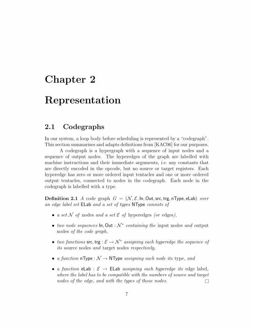
Definition 2.1 A code graph G = (N , E , In, Out, src, trg, nType, eLab) overan edge label set ELab and a set of types NType consists of
• a set N of nodes and a set E of hyperedges (or edges),
• two node sequences In, Out : N ∗ containing the input nodes and outputnodes of the code graph,
• two functions src, trg : E → N ∗ assigning each hyperedge the sequence ofits source nodes and target nodes respectively,
• a function nType : N → NType assigning each node its type, and
• a function eLab : E → ELab assigning each hyperedge its edge label,where the label has to be compatible with the numbers of source and targetnodes of the edge, and with the types of those nodes.
7

M.Sc. Thesis – W. Thaller – McMaster – Computing and Software
x
y
fm
1
1
x
state'
stqx
2
1
addr
3
index
4
state
1
Figure 2.1: Simple codegraphs. Left: a codegraph that squares a vector ofnumbers using the SPU instruction fm (floating point multiply); right: a code-graph with the state-affecting store instruction stqx
Definition 2.2 The function consumers : N → P E maps a node to the set ofall hyperedges in whose source list it appears (its consumers). Likewise, thefunction producers : N → P E maps a node to the set of all hyperedges in whosetarget list it appears (its producers).
Definition 2.3 A codegraph is called executable if
• It is acyclic.
• For every edge, an output node is reachable from at least one target nodeof the edge.
• Every node is either an input node or the target node of exactly oneedge.
At the left of figure 2.1, you can see a very simple codegraph that squares onevector of four floating point values using the SPU instruction fm, floating pointmultiply. To make the figures easier to talk about, we will label each nodein the codegraph with a unique name; remember, however, that nodes in thecodegraph actually only have types, not names. The codegraph in the figurehas two nodes, which we name x and y , and one edge, labeled with the SPUinstruction. The sequence of input nodes contains only x , and y is the only
8

M.Sc. Thesis – W. Thaller – McMaster – Computing and Software
output node. The input and output sequences are visualised by the numberedtriangles connected to the nodes in the figure. The triangles themselves arenot nodes or edges of the graph.
The set of possible types consists of one type for each type of registeravailable in the target architecture — in the case of the Cell SPU, there is justone type of register —, and the type state.
The state type exists to account for the fact that some machine in-structions cannot be modelled as functions from input values to output values;examples include load, store, and branch hint instructions; we do not supportactual branch instructions in the code graph. A value of type state is a tokenthat represents all the state that can be affected by an instruction, includ-ing, but not limited to, memory (in our case, the Cell SPU’s local store), andthe state of the branch processor (which is affected by the hint for branchinstruction).
A state-affecting instruction, like the store instruction stqx (store quad-word indexed) shown on the right of figure 2.1, is then modelled as taking anadditional parameter of type state, and returning a modified state. The figuresuse slanted text to distinguish nodes of type state, like state and state’, fromnodes of the register type, like addr.
Sometimes, we want to work with independent aspects of state, e.g.with different, non-overlapping areas of memory, without imposing a sequentialordering on the instructions that work with different state. In this case, wewill just use two separate state tokens in the codegraph. Use of two separatestate tokens is taken as an assertion that the operations on the two separatetokens are independent from each other; this assertion is not checked by oursystem.
To help describe transformations of codegraphs, we use a theory basedon category theory, more specifically on gs-monoidal categories; this is de-scribed in detail in [KAC06]; for the purposes of this thesis, it is sufficient tosummarise the algebra defined by that theory without requiring any furtherunderstanding of category theory.
Every codegraph G has a signature which consists of the sequence ofthe types of its input nodes and the sequence of the types of its output nodes;it is written as G : I → O . Type sequences can be concatenated using theassociative operator ×; the empty type sequence, denoted by 1l, is both a rightand left unit for ×.
For two codegraphs G : A → B and H : B → C , the codegraphdenoted A;B : A → C is their sequential composition; G ’s output nodes areidentified with H ’s input nodes.
9

M.Sc. Thesis – W. Thaller – McMaster – Computing and Software
Two codegraphs G : A → B and H : C → D can also be composed inparallel using the ⊗ operator, producing G ⊗ H : A× C → B × D .
For a type sequence T , we can construct several basic codegraphs thatdo not contain any edges:
• IT : T → T is the identity codegraph over that type sequence; it containsno edges, and each of its nodes is both an input node and an output nodein the corresponding position, with the types taken from T . The identitycodegraph is both a right and left unit for sequential composition.
• ∇T : T → T×T is a codegraph without operations that “duplicates” itsinput; the list of output nodes equals the list of input nodes concatenatedwith itself.
• As a generalisation of the above, ∇nT : T → T × T n is a codegraph
without operations that replicates its input n times; the list of outputnodes equals the list of input nodes concatenated with itself n times.
• !T : T → 1l contains distinct input nodes, and nothing else. Informallyspeaking, it ignores its input and produces no output.
2.2 Loop Specifications
To specify a loop, rather than just a loop body, we need to specify what valuesare communicated between different iterations of the loop.
Definition 2.4 A loop specification is a tuple (G ,d) containing
• an executable codegraph G : F ×K → F × C
• a sequence of integers d, one for each element of F .
The input of the codegraph consists of two parts; for the left part,with types F , there are corresponding outputs and an associated integer d .These inputs and outputs represent the values that are communicated betweendifferent iterations of the loop. In any iteration i , the value of each of theseinputs is equal to the value of the corresponding output in iteration i + d .
Hence, the usual case of using an output from the previous iteration isrepresented by d = −1. A value of d of less than −1 means that the input forthe codegraph should be an output from further back in the past; this can,for example, be achieved by storing the value in an array so that it won’t beoverwritten by the next iteration.
10

M.Sc. Thesis – W. Thaller – McMaster – Computing and Software
A value of d = 0 means that the input should be equal to the outputfrom the same iteration; alternatively, we could just use a single interior nodein place of the input node and the output node.
An input/output pair with an associated d greater than 0 means thatthe input for iteration i should be the output of some future iteration i + d .This is, of course, impossible if the loop is scheduled in the conventional way,without software pipelining. In the presence of software pipelining, schedulingloop specifications with positive d values sometimes becomes possible, as wewill see in chapter 3. For an example of how d values other than −1 might beused in a loop specification, refer to section 2.5.
In addition to the inputs with corresponding outputs (F ), the code-graph G also has another group of inputs, of types K . These inputs are calledconstant inputs and represent all values that are passed to the loop from theoutside but are not changed by the loop; these include unchanging parametersfor the loop and constants that cannot be part of the opcode of a machinelanguage instruction (and therefore included in the label of a hyperedge inthe codegraph). In other words, the constant inputs are those values that arerequired to be available in a register when the loop starts and throughout theexecution of the loop.
Finally, G also has a group of outputs of types C , called the controloutputs. These control outputs are used to control when the loop shouldterminate; their meaning is described in more detail in section 2.4.
2.3 Maximum Lifetime and Loopability
We impose one additional restriction on the scheduler’s output: Every opera-tion in the codegraph must appear exactly once in the scheduled loop body,and every instruction in the scheduled loop body must appear in the code-graph. We do not want the scheduler to insert additional instructions, likeextra register-to-register moves.
As a consequence, a node in the codegraph will be assigned to at mostone register for its entire lifetime. The lifetime of one node in one iteration alsocannot overlap with the lifetime of the same node in another iteration (that isbeing executed at the same time due to software pipelining); we make it theduty of the scheduler to limit the lifetimmes to less than λ, so that modulovariable expansion is never required.
Forbidding long lifetimes can have a negative impact on the achieved λ.However, as the codegraph does not explicitly specify locations for temporaryvalues, modulo variable expansion becomes nothing but a fancy term for loop
11

M.Sc. Thesis – W. Thaller – McMaster – Computing and Software
unrolling; we can therefore achieve the effects of longer lifetimes and modulovariable expansion by replicating the loop body a few times before running thesoftware pipeliner.
This has the advantage that we can always avoid having to use modulovariable expansion, which is crucial for scheduling multiloops (see chapter 6).
Not all loop specifications can be scheduled as loops without addingextra instructions. First, we consider the situation without software pipelining,i.e. when all operations scheduled in the loop body must operate on databelonging to the same iteration.
If an input node in the codegraph is also an output node, then theymust be an input and an output in corresponding positions in F . The valueof the node then has to be the same for all iterations; the input-output paircan therefore be converted to a constant input by removing the node fromthe output sequence of the codegraph and moving its position in the inputsequence to the right to make it part of K rather than of F .
The case where a node is both an input and the corresponding outputis easy to avoid by making it a constant instead; in other cases it is easyto explicitly specify an appropriate register-to-register move instruction. Wetherefore require the input codegraph to have no input node that is also anoutput.
If a value is calculated by an instruction in iteration i , the same in-struction in iteration i + 1 will overwrite it with a new value. Therefore, toachieve d < −1, an additional instruction has to be added to move the valueto some other location before it gets destroyed.
Positive values for d are impossible: Using results from iteration i +d , d > 0 in iteration i requires iteration i + d to start before iteration i hasfinished (software pipelining or reordering of iterations).
Definition 2.5 A loop specification is loopable if
• All d are −1 or 0.
• No input is also an output.
An input-output pair with d = 0 is equivalent to identifying the input nodewith the output node (and removing them from the codegraph’s input andoutput sequences). If this transformation succeeds without introducing cyclesinto the codegraph, we get a strictly loopable loop specification:
Definition 2.6 A loop specification is strictly loopable if
12

M.Sc. Thesis – W. Thaller – McMaster – Computing and Software
• All d are −1.
• No input is also an output.
2.4 Loop Termination
Informally speaking, the control outputs (C ) determine whether the loopshould continue after the current iteration. The control outputs are connecteddirectly to the branch instruction at the end of the loop; depending on whatkind branch instruction is used for the loop, they can have different meanings.
For the Cell SPU target architecture, we currently use the followingvariants:
• The loop branch is a brnz (branch if not zero word) instruction; the loopcontinues if the first component of the only control output (which is, asare all values on the SPU, a vector) is non-zero.
• The loop branch is a bi (branch indirect) instruction; the first componentof the only control output should contain the address of either the firstinstruction of the loop or of the first instruction after the loop.
• The loop branch is a bi instruction, as above; additionally, a secondcontrol output is a state token that is generated by a hbr (hint for branch)instruction.
2.5 Example
As a toy example, let us specify and schedule a loop that takes an array offloating point numbers as input and writes the square of every element toa separate output array. We can start with the codegraph from Figure 2.1,but to get a loop, we need to add instructions to load values from the inputarray, store values to the output array, update a loop counter, and calculate aloop condition as an output of the codegraph. The actual branch instructionwill not be part of our codegraph (after all, we do not need an instructionscheduling algorithm to tell us that the branch instruction should occur rightafter the end of the loop body).
Figure 2.2 shows a loop specification for this loop; the d vector for theloop specification is visualised by adding dashed, labelled arcs from the outputto the corresponding input in the codegraph. The instruction lqd 0 loads avector from the SPU’s local store; its inputs are a state token and the address
13

M.Sc. Thesis – W. Thaller – McMaster – Computing and Software
counter
counter'
inState
inState'
outState
outState'
ptrDiff
x
y
21
3 4
21
3
fm
stqx
lqd 0 ai 16-1 -1
-1 rotqbyi 4
continue
4
Figure 2.2: Loop that squares all elements in an array
of the vector to load, and its outputs are a state token and the vector thatwas loaded. For storing a vector, we use the stqx instruction; its inputs area state token, the value to be stored, and two values which are added to yieldthe target address in the SPU’s local store. We use separate state tokens forloading and storing, which are both passed on from one iteration to the next(d = −1).
The loop counter is incremented by 16 (the size in bytes of a vectorvalue) in every iteration using the ai 16 instruction and passed on to thenext iteration (d = −1). We play a little SPU-specific game here: we takeadvantage of the fact that all values on the SPU are vectors, and the ai
instruction separately affects all four 32-bit components of the register. Weinitialise the first component of the vector to the address of the input array(the lqd and stqx instructions always use the first component of their addressarguments). The last component will contain −16n, where n is the number of
14

M.Sc. Thesis – W. Thaller – McMaster – Computing and Software
times the loop should be executed; it will reach zero after the nth iteration.The stqx instruction stores the vector y at the address that results from
adding the first components of the vectors ptrDiff and counter’. It consumesthe state token outState and produces a new state token, outState’.
Finally, the instruction rotqbyi 4 rotates the vector so that the lastcomponent is moved to the first component, where it is needed for the condi-tional branch.
The values counter and counter’ will occupy the same register (other-wise, we would need to insert a register-to-register move instruction), so thereis a data antidependence between the stqx and the ai 16. The stqx has tobe scheduled before the ai because an input it needs (counter’) is destroyedby ai.
We can now estimate a lower bound for the number of cycles this loopwill take without software pipelining; we need to add up latencies, plus onecycle for the antidependence between stqd and ai:
6 (lqx) + 6 (fm) + 1 (antidependence) + 2 (ai) + 4 (rotqbyi) = 19
Nineteen cycles is nothing to be proud of for a loop with just fiveinstructions. The throughput can be increased by unrolling the loop or byapplying software pipelining.
To make software pipelining this loop easier, we can also consider de-riving the loop condition and the store address from the counter values for adifferent iteration, as shown in Figure 2.3. The value counter’ is now mentionedtwice in the output list of the codegraph; one occurence still corresponds to thecounter input with d = −1, that is, counter in iteration i is the value computedby the ai instruction in iteration i−1. The other counter’ output correspondsto a new input counter”, which, in iteration i , is the value computed by theai instruction in iteration i + x .
This loop specification is not semantically equivalent to the earlier one;we need to adjust the ptrDiff and the initial value of counter according to thevalue of x .
15

M.Sc. Thesis – W. Thaller – McMaster – Computing and Software
counter
counter'
inState
inState'
outState
outState'
ptrDiff
x
y
21
3 5
21
3
fm
stqx
lqd 0 ai 16-1 -1
-1 rotqbyi 4
continue
5
counter''
4
4
x
Figure 2.3: Improved Loop for Software Pipelining — use x > 0 to facilitatesoftware pipelining
16

Chapter 3
Theory of Staging
Software pipelining can be viewed as a transformation of the loop specification.Informally speaking, we split up the codegraph into sequential parts, which wecall stages, and compose them again in parallel to get a new loop body suchthat adding appropriate prologue and epilogue code to the loop yields a loopthat is equivalent to the original loop.
For the purposes of this chapter, we assume a legal assignment to stagesto be given; a stage assignment is legal when the transformation outlined inthe next section can transform the loop specification (G ,d) to a loopable loopspecification (G ′,d′). Chapter 4 describes an algorithm for calculating a legalstage assignment for a loop specification.
Consider a loop that we can split into three stages, G1, G2 and G3.In figure 3.1, Gi ,j denotes stage Gi operating on data for logical iterationj . If we schedule the loop without software pipelining (figure 3.1, left), theloop independent data dependences between the stages will prevent us fromexploiting much parallelism. With software pipelining (figure 3.1, right), thesedependences are between different iterations of the pipelined loop and thereforedo not restrict parallelism between the stages.
Figure 3.2 shows how different values of d can be realised in a pipelinedloop. When we assign operations to stages (chapter 4), we will need to assignstages in such a way that the resulting assignment is legal :
Definition 3.1 A stage assignment with k stages for a given loop specificationis considerd legal iff the following conditions are fulfilled:
• Every operation in the code graph is assigned to exactly one stage in therange 1 . . . k.
17

M.Sc. Thesis – W. Thaller – McMaster – Computing and Software
G1,0
G1,1 G2,0
G1,2 G2,1 G3,0
G1,3 G2,2 G3,1
G1,n-1 G2,n-2 G3,n-3
G2,n-1 G3,n-2
G3,n-1
…
G1,0
G1,1
G2,0
G1,2
G2,1
G3,0
G1,3
G2,2
G3,1
G1,n-1 G2,n-1 G3,n-1…
G2,3
G3,2
G3,3
Prologue
Epilogue
j = 0
j = 1
j = 2
j = 3
j = n-1
j' = 0
j' = 1
j' = n-3
Figure 3.1: Software pipelining with three stages; left: loop independent datadependences in a non-pipelined loop restrict parallelism; right: the same de-pendences are now dependences between different iterations of the pipelinedloop.
• A value produced by an operation in stage i can be consumed by opera-tions in stage i and/or in stage i + 1.
18

M.Sc. Thesis – W. Thaller – McMaster – Computing and Software
G1,j-1 G2,j-2 G3,j-3
G1,j G2,j-1 G3,j-2
-1 -3
2
Figure 3.2: Inter-iteration dependences in a pipelined loop
• For an input/output pair where the output value is produced by an oper-ation in stage i, the input value can be consumed by operations in stagesi + d and/or in stage i + d + 1.
It is tempting to simply split up the codegraph G into k sequentiallycomposed subgraphs, the stages Gi :
G = G1;G2; . . . ;Gk
and then to recompose them in parallel:
G ′ = P ;(G1 ⊗G2 ⊗ . . .⊗Gk),
where P is a permutation to make the argument order of the codegraph matchup. We would then pick an appropriate d′ to make a new loop specification.
This approach, however, gets us no closer to actually scheduling asoftware-pipelined loop, as we are potentially violating both conditions forbeing loopable. For one, we have no way of guaranteeing that −1 ≤ d ′ ≤ 0.Also, output values that are computed in one stage have to be passed throughthe later stages in the sequential composition, and inputs have to be passedthrough the stages before the one where they are consumed.
3.1 Pipelining Transformation
We want to do the sequential decomposition in a way that connects inputsconsumed and outputs produced in a stage Gi directly to the inputs and
19

M.Sc. Thesis – W. Thaller – McMaster – Computing and Software
outputs of G as a whole, without routing them “through” the other stages.
The individual stages will be
Gi : Mi−1 × Ii ×Ki → Oi × Ci ×Mi
The Ii inputs of each stage are inputs from F , the Ki are constantsfrom K , and Mi−1 are outputs from the previous stage. Likewise, the Oi andCk are connected to the output of G , while the Mi are fed into the next stage.
Due to the obvious lack of a stage before the first stage or a stage afterthe last stage, M0 = Mk = 1l. Furthermore, we want all control outputs tobe generated in the same stage c, so we define Ci = 1l for all i 6= c, andCc = C . The “control stage number” c becomes an additional parameter forthe software pipelining and influences the meaning of the control outputs; seesection 3.3 for details.
Because every output node has exactly one producer in G , every ele-ment of F will appear in the output list Oi of exactly one stage Gi ; inputs,however, can appear in the Ii lists more than once.
We will also have to add a codegraph without any operations at thetop to rearrange the Ii and Ki to match the order of F × K , and to do thesame at the bottom to make the order of the Oi match up with F × C :
G = P ;(G1 ⊗ II2×...×Ik );(IO1 ⊗G2 ⊗ II3×...×Ik ); . . . ;(IO1×...×Ok−1⊗Gk);Q ,
The codegraph P : F × K → (I1 × K1) × . . . × (Ik × Kk) has no hyperedges;it will route each input to the place or places (if any) where it appears inthe input lists of the individual stages; constant inputs can appear on P ’soutput list any number to times, other inputs up to twice. The codegraphQ : O1 × . . . × Ok → F × C is a permutation, i.e. a codegraph withoutoperations whose nodes each appear exactly once on its input sequence andexactly once on its output sequence. Figure 3.3 illustrates how three stageswould fit together.
If the stages Gi have been chosen appropriately, we can construct anew, loopable, software pipelined loop specification (G ′,d′) where the stagesare executed in parallel, but for different “logical iterations”, i.e. for differentiterations of the original loop specification.
We have stated before that an input value from F can be used in morethan one stage.
In every iteration of a software pipelined loop, the value of an input inF for two different iterations; if at the top of the pipelined loop, the value isavailable for some logical iteration j , then at some later point in the schedule,
20

M.Sc. Thesis – W. Thaller – McMaster – Computing and Software
P
Q
G1
G2
G3
M1
M2
O3
O2
O1
I1
I2
I3
O1 O2
I3I2
F K
CF
C3
Figure 3.3: Splitting a codegraph into three stages
there will be an instruction that produces the value for iteration j +1, replacingthe value for iteration j .
In the pipelined loop, stage i will operate on logical iteration j +1 whilestage i + 1 is still working on logical iteration j . Stage i can access the valueof the input for logical iteration j +1 if the consuming instruction is scheduledbelow the producer; in the same iteration of the pipelined loop, stage i +1 canaccess the value for logical iteration j if the consuming instruction is scheduledabove the producer. No other stages have access to a value of the input forthe logical iteration they are working on.
Therefore, every input value from F can be used by at most two con-secutive stages; the corresponding output value appears exactly once in theOi list of exactly one stage, but it must appear twice in the output list ofG ′. One appearance will be associated with a d ′ = −1 entry in d′, the otherappearance with d ′ = 0.
Unused inputs are permissible in codegraphs, so we can simply do thisfor all outputs, even if they are used only once. We define
21

M.Sc. Thesis – W. Thaller – McMaster – Computing and Software
R
G1 G2 G3
M1O1
I1 I3I2
F' K
O1 O1
M1 M2
M2O2
O2 O2
CO3
O3 O3
O1 O1 O2 O2 O3 O3M1 M2
CF'
Figure 3.4: Putting the stages together in parallel
G ′i = Gi ;(∇Oi ⊗ ICi ⊗ IMi )
The kernel G ′ : F ′ × K → F ′ × C of the software-pipelined loop willthen be
G ′ = R;(G ′1 ⊗ . . .⊗G ′
k);S ,
where F ′ = O1×O1×M1×. . .×Ok×Ok , and S : O1×O1×C1×M1×. . .×Ok×Ok ×Ck → F ′×C and R : F ′ → I1×K1×M1× I2×K2× ...×Mk−1× Ik ×Kk
is a codegraph without operations.S is constructed such that it moves the C outputs to the end of the
output list; if the control stage is the last stage (c = k), then S = IF ′×C .Figure 3.4) shows how these parts fit together for k = c = 3.
The entries in d′ will be 0 for each first instance of Oi outputs, and −1for the second instance of Oi outputs and for the Mi . We will choose R suchthat:
• Every Mi input is mapped to the corresponding Mi output; the corre-sponding d ′ value is −1.
• If P maps an input from K to an element of Ki , then R will map thatsame input from K to the same element of Ki (which will, in general,
22

M.Sc. Thesis – W. Thaller – McMaster – Computing and Software
not be in the same position in the output of R as it is in the output ofP).
• The first occurence of each Oi input is mapped to the correspondingoutput in Ii+d , if such a corresponding output exists, where d is thevalue associated with Oi in the original loop specification.
• The second occurence of each Oi input is mapped to the correspondingoutput in Ii+d+1, if such a corresponding output exists.
3.2 Prologue and Epilogue
The software-pipelined loop specification is not a drop-in replacement for theoriginal loop; after all, it requires intermediate results (Mi) as its input, whichhave to be supplied to the first iteration of the modified loop body. We do thisby prefixing the modified loop with a prologue, a block of non-looped codethat initialises the pipeline, as we see in the pipelined loop shown on the rightof figure 3.1.
The first time the modified loop body executes, it will execute Gk forlogical iteration 0, Gk − 1 for logical iteration 1, and G1 for logical iterationk−1. The prefix code, therefore, has to execute G1 . . .Gk−1 for logical iteration0, G1 . . .Gk−2 for logical iteration 1, and so on.
Likewise, after the last iteration of the software pipelined loop body,some logical iterations have been started but not finished. If the softwarepipelined loop body has been executed n − k + 2 times, the latest logicaliteration that has been completed will be n− k −3; logical iterations n− k +2through n will have been initiated but not completed. The epilogue code needsto execute Gk for iteration n− k +2, Gk−1 and Gk for iteration n− k +3, andso on, and finally G2 through Gk for iteration n.
Every iteration of the loop uses output values from earlier iterations asinputs, so when the loop starts at logical iteration 0, values have to be suppliedfrom the outside, as there are no iterations with negative indices. If an inputis associated with a d value of less than −1, multiple “initial” values for theinput have to be supplied, corresponding to the outputs of the non-existantiterations d through −1. Inputs with nonnegative values for d , on the otherhand, do not need any initial values at all.
Figure 3.5 shows how the loop gets initial values that are conceptuallythe outputs of negative iterations; only the values originating from stage 3 ofiteration −3 and from stage 2 of iteration −1 are shown in the figure. Not
23

M.Sc. Thesis – W. Thaller – McMaster – Computing and Software
G1,0 G2,-1 G3,-2
G1,1 G2,0 G3,-1
G1,2 G2,1 G3,0
G1,-1 G2,-2 G3,-3
Figure 3.5: Prologue of loop with three stages. Initial values from G3,−3 andG2,−1 are shown as arrows.
all the outputs from those stages are required for loop initialisation; some areonly required by other negative iterations (dashed arrows).
To construct a codegraph for the loop prologue we first define init(x )to be the primitive codegraph consisting of one hyperedge labeled with initx ,with no inputs and exactly one output. Using that, we define
Gi ,j = Gi if j ≥ 0Gi ,j = !Mi−1×Ii×Ki
;(init(i , j , 1)× . . .× init(i , j , |Ii ×Mi × Ci |)) if j < 0
Here, i is the stage number and j is the logical iteration. For negative j , we donot want to generate any code; instead of the codegraph Gi for the stage, weconstruct a codegraph with the same input and output types that ignores allits inputs, and whose outputs are the results of hyperedges specially markedwith the stage, iteration and position of the output.
We then continue with
G ′i ,j = Gi ,j ;(∇Oi × ICi × IMi ),
so that we can define one slice of the prologue
Prj = R;(G ′1,j ⊗ . . .⊗G ′
k ,j−k+1);S .
24

M.Sc. Thesis – W. Thaller – McMaster – Computing and Software
We resolve all d ′ = −1 by identifying the corresponding input and outputnodes, and removing them from the input and output lists. Let the results ofthis transformation be Pr ′j : F ′′×K → F ′′×C . We ignore the control outputsfrom the prologue:
Pr ′′j = Pr ′j ;(IF ′′⊗!C )
Next, we compose Pr ′′−1 . . .Pr ′′k−2 sequentiallly, supplying a copy of the constantinputs to each:
Pr ′ = (IF ′′ ⊗∇kK );(Pr ′′−1 ⊗ IK (k−1));(Pr ′′0 ⊗ IK (k−2)); . . . ;Pr ′′k−2
Then, we remove all unused nodes and edges from which no output isreachable from Pr ′, except for the constant inputs; this makes the codegraphexecutable again. Finally, we remove all init-labelled hyperedges and maketheir target nodes inputs of the prologue (the labels of the init hyperedges nowdefine the meaning of those inputs).
Construction of the epilogue is symmetric to construction of the pro-logue.
3.3 Loop Termination Revisited
In a software pipelined loop, we have little choice but to interpret the controloutputs based on the pipelined loop body; therefore, their meaning changesdepending on the value of c, i.e. depending one which stage they are producedin.
If the control outputs evaluate to a value meaning “do not continue”in stage c of iteration n, then, the last iteration of the pipelined loop executesG1,n+c−1, . . . ,Gc,n , . . . ,Gk ,n+c−k . Including the loop epilogue, the last iterationto be executed will be iteration n + c − 1.
If we are trying to save on code size, we can do without an epiloguealtogether in many cases; we might need to provide some extra space forpartial results in any memory areas that the loop stores its results in. Withouta prologue, if iteration n causes loop termination, the last iteration to becompleted is iteration n + c − k ; additionally, iterations n + c − 1 throughn + c − k + 1 have been initiated, but not finished. It will depend on theparticular stage assignment chosen for this loop whether any results for thosepartial iterations will be stored to memory or not.
25

M.Sc. Thesis – W. Thaller – McMaster – Computing and Software
3.4 Correctness
This thesis does not concern itself with a formal proof that the pipeliningtransformation and the prologue/epilogue construction yield a transformedloop that is equivalent to the original.
However, we can observe that every stage appears is executed the samenumber of times in the original loop and in the pipelined loop with prologueand epilogue. Also, the codegraph R (which governs how the inputs of thepipelined loop body are arranged) is constructed at the end of section 3.1 toalways match up the corresponding inputs and outputs, and taking the ap-propriate d values into account. The transformation makes some assumptionsabout the assignment of operations to stages, which are all covered by thedefinition of a legal stage assignment given in the introduction to this chapter.
3.5 Example
Let us now return to our earlier example and have a look at how we canstage the loop specification from figure 2.3 on page 16; this is the variantwhere we can choose a parameter x that will tell the store instruction and theloop condition to use the loop counter from a different iteration. We will usethis loop specification instead of the more straightforward one from figure 2.2because it is much more amenable to software pipelining.
If we schedule the stqx two stages or more after the lqd, then thecounter value will already have been updated in the meantime; the value forthe current iteration will not be available any more. In its place, however,there is the counter value of a later iteration ready for use in the same register.Setting x to a value greater than −1 will therefore allow the load and storeinstructions to be farther apart.
With x = 1, the stqx and rotqbyi instructions that use counter” canbe two or three stages after the ai instruction that produces them. If wedecide on a total of three stages, this means that the ai instruction will bein the first stage, and the stqx and rotqbyi instructions will be in the laststage.
Figure 3.6 shows how the codegraph can be split up into three sequen-tially composed stages. In the example at hand, P ends up being an identitycodegraph because the inputs used by stage 1 happen to be listed before theinputs used by stage 3 in the input sequence of the original codegraph.
The loop can then be pipelined by recomposing the stages in parallel,as shown in figure 3.7. The vertical positions of the operations indicate where
26

M.Sc. Thesis – W. Thaller – McMaster – Computing and Software
counter
counter'
inState
inState'
outState
outState'
ptrDiff
x
21 3
fm
stqx
lqd 0 ai 16
rotqbyi 4
continue
5
counter''
4
y
1 2 3 4 5
Stage 1
Stage 2
Stage 3
Q
P
Figure 3.6: Splitting up the loop into three stages. d = (−1,−1,−1, 1)
they occur in the final schedule. None of the inputs with d ′ = 0 (shownslightly above and to the left of the inputs with d ′ = −1) are actually usedin this example; the nodes a, b, c and d are not used by any operations.Transforming the loop specification to a strictly loopable loop specificationwill therefore simply remove them and their corresponding outputs.
The scheduled loop body takes just 7 cycles to execute; this is just onecycle longer than the latency of the multiply and load instructions, and is anoptimal schedule for this code.
27

M.Sc. Thesis – W. Thaller – McMaster – Computing and Software
counter
counter'
inState
inState'
outState
outState'
ptrDiff
x
y
54 10
fm
stqx
lqd 0
ai 16
rotqbyi 4
continue
11
counter''
6
x
7 8
y
54 10 116 7 8
21 3 9
21 3 9
a b c d
Stage 1 Stage 2 Stage 3
R
Figure 3.7: Pipelined loop, with three stages.d′ = (0, 0, 0,−1,−1,−1,−1,−1, 0,−1)
28

Chapter 4
Heuristic Staging
We will now present a heuristic algorithm for splitting up a given loop speci-fication into k stages. This means assigning a stage number in the range 1..kto each hyperedge in the given codegraph.
In addition to having to find a legal stage assignment, we want to avoidpartitioning the codegraph in such a way that:
1. The latency along the longest path through one of the stages is greaterthan the initiation interval we expect to achieve.
2. Too many registers are alive accross stages.
All registers that are alive accross stages will be live at the top of thefinal scheduled loop and will therefore conflict with each other. On theother hand, higher register requirements inside a stage can be mitigatedby good decisions in the later steps.
3. Too many forward dependences between stages arise between stages.
An inter-stage forward dependence corresponds to an input/output pairin the pipelined loop specification for which the associated d ′ = 0. Thisis generally undesirable, because it reduces parallelism between the in-volved stages; it is especially undesirable when we use the merge schedul-ing algorithm (chapter 5) which cannot handle forward dependences well.
The heuristic method we are going to use is based on using two functions,depth and height, that map every operation in the code graph to a nonnegative“depth” and “height” value.
We will use the depth and height values to decide approximately whereto cut the codegraph into stages. More restrictions are placed on where to split
29

M.Sc. Thesis – W. Thaller – McMaster – Computing and Software
based on the dependences between the operations; finally, from the cuts thathave not been eliminated earlier, we pick the one that minimises the numberof values communicated from one stage to the next, i.e. we minimise registerrequirements at the top of the loop.
The algorithm proceeds as follows:
1. Initialise a constraints graph S (see section 4.2) that contains our currentknowledge about the stage assignment.
2. For i := k down to 2
(a) Calculate height, depth, htot , and dtot based on the codegraph withall operations known to be in stage i + 1 or greater removed (seesection 4.1)
(b) Try to mark all operations with height > htot/i as being in stagei − 1 or less
(c) Try to mark all operations with depth > (i − 1)dtot/i as being instage i
(d) Let A be the set of all opoerations known (according to S ) to be instage i − 1 or less, and let B be the set of all operations known tobe in stage i or greater
(e) Construct Gcut (see section 4.3)
(f) Run a minimum cut algorithm on Gcut
(g) Mark all operations in Gcut that are above the minimum cut asbeing in stage i − 1 or less
(h) Mark all operations in Gcut that are below the minimum cut asbeing in stage i or greater
3. Extract final stage assignment from S .
4.1 Height and Depth
There are several choices for the depth and height functions. The simplest isto calculate depth and height based on the latencies of instructions:
Definition 4.1 Given a codegraph G,
30

M.Sc. Thesis – W. Thaller – McMaster – Computing and Software
• For all n ∈ N , depthL(n) is the depth of the producer of n plus theproducer’s latency, or 0.
• heightL(n) is the maximum of the heights of all consumers of n plus theirrespective latencies, or 0.
• For all e ∈ E, depthL(e) is the maximum of the depths of all sources ofe.
• heightL(e) is the maximum of the heights of all targets of e.
For an operation (a hyperedge) e in the codegraph, the function depthL(e)gives a lower bound on the number of cycles that pass between the initiation ofan iteration and when the instruction is issued for that iteration in a softwarepipelined schedule. Likewise, heightL(e) gives a lower bound for the number ofcycles that pass between the completion of the instruction and the completionof the last instruction in the iteration.
Definition 4.2 Given a codegraph G,
• For all e ∈ E, heightU (e) is the number of hyperedges e ′ that are reachablein G from e and for which unit(e ′) = u when u is chosen such thatheightU (e) becomes maximal.
• depthU (e) is the number of hyperedges e ′ that are reachable in reversedirection from e and for which unit(e ′) = u when u is chosen such thatdepthU (e) becomes maximal.
The lower bounds provided by heightU (e) and depthU (e) stem from thefact that only one instruction per unit can be executed in one machine cycle;all edges reachable from e have to be executed after it, and all nodes reachablein reverse direction have to be executed before it.
To get the “best of both worlds”, we therefore define
Definition 4.3 For all e ∈ E, heightLU (e) = max (heightL(e), heightU (e)) anddepthLU (e) = max (depthL(e), depthU (e)).
Definition 4.4 Furthermore, we define a total height htot and a total depthdtot :
• htot = maxn∈N height(n)
• dtot = maxn∈N depth(n)
31

M.Sc. Thesis – W. Thaller – McMaster – Computing and Software
4.2 Stage Constraints
Let s be the function that maps each operation to its stage number. Duringthe execution of the algorithm, a directed graph S will represent our currentknowledge about this function. Its nodes are the operations in G , plus anadditional node z . We define s(z ) = 0. An edge (x , y , d) (an edge from x toy , labeled with the integer d) is taken to denote the constraint
s(x ) + d ≥ s(y).
Due to the transitivity of ≥, the shortest path SP(x , y) between two nodescan be used to derive new constraints.
∀ x , y : s(x ) + SP(x , y) ≥ s(y)
Specifically, we get:
∀ x : −SP(x , z ) ≤ s(x ) ≤ SP(z , x )
Initially, we populate the graph with edges representing the constraints wealready know:
• Edges to and from z to enforce ∀ x : 0 ≤ s(x ) < k
• For every edge (x , y , d) in the dependency graph, edges (x , y , d + 1) and(y , x ,−d)
• Edges forcing all producers of control outputs to be in the last stage.
Then, we add some more constraints that are likely to yield a better stageassignment:
• Edges forcing the operations with the greatest height to be in the firststage.
This is essential for making the stage assignment yield good results.
• For each non-constant input, edges forcing all its consumers to be in thesame stage.
This constraint serves to subtly discourage, but not entirely forbid inter-stage forward dependences (d ′ = 0 in the pipelined loop specification).
32

M.Sc. Thesis – W. Thaller – McMaster – Computing and Software
These constraints are not logically necessary, and as such can cause negative-weight cycles in S if they contradict other constraints. Therefore, if adding anedge for one of these constraints would create such a cycle, the constraint issimply ignored.
The algorithm then decides the boundaries between stages one by one,starting at the last stage. The number of the stage below the boundary to bedecided shall be denoted by i .
For each boundary, the height and depth functions are used to clas-sify each operation into three categories: above, below and undecided. Theprimary aim here is to exclude stage assignments that violate the second con-dition stated above, i.e. assignments where one of the stages, when scheduledindividually, is longer than we would like our final loop body to be.
We calculate the height and depth functions based on a subgraph ofthe codegraph G ; all nodes that are (according to S ) known to be in stagei + 1 or below are excluded. Thus, the total height and depth correspond toall the instructions from the first stage to stage i , inclusively.
Rather than pre-determining a target λ, we just strive to split up thecodegraph into stages of roughly equal size, as measured by the height anddepth functions. As the height function is intended to give a lower bound of thedistance in cycles between an instruction and the “bottom” of the codegraph,we force all operations with a height greater than htot/i to be in stage i − 1or above; likewise, all instructions with depth greater than (i − 1)dtot/i to bein stage i .
The graph S is augmented to reflect this new information by addingthe appropriate edges to and from z . If adding such an edge would create acycle with negative weight in S , then it is skipped. This means that previousdecisions, or their consequences, contradict the new “recommendation” thatwas derived from the height and depth functions. Precedence has to be givento the earlier decisions.
We can now extract the set of all operations whose position with respectto the stage boundary under consideration is not yet known from the graph S .The exact boundary is then determined in a way that minimises the numberof registers required (as described below). The results of that decision is thenrecorded in S again, and the process repeated for the next lower-numberedboundary, until all stages are decided.
33

M.Sc. Thesis – W. Thaller – McMaster – Computing and Software
4.3 Stage Separation
Now let us turn to the problem of determining where to draw the exact bound-ary between two stages. We have already narrowed down our choice so thatcondition 1 will always be fulfilled.
The goal now is to find a partitioning that fulfills the other two con-ditions, i.e. one that minimises register use without violating any of the con-straints and without generating too many forward dependences. Of course,we must still make sure that our choices don’t violate any other constraintsdefined in the previous section.
We can do this by transforming the remaining codegraph (after re-moving the nodes that are already known to be either above or below theboundary) to an instance of the minimum cut problem; the minimum cut willbe the stage boundary that uses the smallest number of registers at the top ofthe loop.
We want to define a graph Gcut such that:
1. A minimum cut yields two stages with no illegal dependences.
2. The size of the minimum cut equals the number of values that have tobe kept in registers from one stage to the next.
Definition 4.5 Given a codegraph G, we first define a graph G ′cut containing
• A “source” node s
• A “sink” node t
• For every operation in the codegraph, an “operation” node
• For every node in the codegraph, a “value” node
• An edge with infinite weight from each consumer of a value to the pro-ducer
• An edge with weight 1.0 from each producer to the corresponding valuenode
• An edge with infinite weight from each value node to each of its con-sumers.
34

M.Sc. Thesis – W. Thaller – McMaster – Computing and Software
minimum cutknown above
known below
A
b
a
B
C
D
c
d e
b
1.0
B
C
c
d e
∞
1.0
∞
1.0
∞
1.0
∞
∞
∞
∞
∞
s
t
e
Figure 4.1: Transforming parts of a codegraph (left) to a minimum cut problem(right). Edges A and D are known to be above and below the stage boundarybeforehand; using the minimum cut we decide to put B and C below the cut,because that requires the least number of registers to be live at the top of thestage.
Definition 4.6 Based on G ′cut , a set A of operations (hyperedges in the code-
graph) known to be above the boundary, i.e. in stage i − 1 or less, and a setB of operations known to be below the boundary, i.e. in stage i or greater, wedefine a graph Gcut by
• Deleting all operation nodes in A ∪ B
• Deleting all value nodes that are not connnected to a consumer or pro-
35

M.Sc. Thesis – W. Thaller – McMaster – Computing and Software
ducer not in A ∪ B
• Deleting all edges that connect two deleted nodes
• Replacing all mention of nodes in A in the remaining edges with s
• Replacing all mention of nodes in B in the remaining edges with t
Figure 4.1 illustrates this transformation on a simple example.If at least one of the consumers of a value is above the cut, then the
producer must also be above the cut. This is easily achieved by having an edgewith infinite weight point from each of the consumers to the producer; any cutwhere the producer is below the cut but one of the consumers is above wouldtherefore have infinite weight, and therefore cannot be the minimum cut.
A value is live at the top of the loop if the operation that produces itis above the cut and at least one of the consumers is below the cut. For everyvalue, we want an edge with weight 1.0 that crosses the cut if and only if thevalue is live at the top of the loop. We only want one such edge per value inorder to avoid counting any live value twice. Therefore, this edge with weight1.0 connects the producer node to the value node; edges with infinite weightare used to connect the value node to each of its consumers. Note that thereis no edge going from the consumer to the value, so that it is possible for avalue node to be below the cut while the operation node that consumes thevalue is above the cut.
We express the constraint that we want all consumers of an input to bein the same stage at this level by adding a cycle of edges with infinite weightbetween all successors of each input.
If a value has a producer or consumer whose stage is already knownand a producer or consumer whose stage is not yet known, the transformationis done as above, but t is substituted for any operation that is known to be instage i or greater, and s is substituted for any operation that is known to bein stage i − 1 or less.
36

Chapter 5
Merge Scheduling
Merge scheduling is based on the idea of “merging” two or more scheduledpieces of code to be executed in parallel. The individual stages we just createdhave relatively few inter-stage dependences, which works in our favour.
Analogous to the use of the term “merging” in the well-known mergesort algorithm, we do not rearrange the instructions in any one input schedulewith respect to other instructions from the same input schedule. Merging canbe done optimally in O(nk+1) cycles, where k is the number of schedules tobe merged and n is the number of instructions involved.
This naturally leads to the following plan for software-pipelining loops:
1. Heuristically assign instructions to stages
2. Schedule the individual stages using a conventional scheduling algorithm
3. “Merge” the individual linear schedules.
5.1 Separate Scheduling
After the stages have been decided, we need to come up with separate schedulesfor each of the stages. For this, we can essentially use any scheduling algo-rithm for straight-line code, as long as we enforce a few additional restrictionsimposed by loop carried dependences.
After staging, loop carried and inter-stage dependences can be classifiedin two groups depending on the value of their associated component in d′, andbased on whether the producing and the consuming instruction are in the samestage or not.
37

M.Sc. Thesis – W. Thaller – McMaster – Computing and Software
• d ′ = 0, same stage
This can only be caused by an input/output pair with d = 0 in theoriginal loop specification. We can eliminate this either before or afterstaging by identifying the input and the output node in the codegraphand removing them from the input and output sequences.
• d ′ = 0, different stages
An inter-stage forward data dependence constraint is passed on to themerging algorithm; no special treatment is required when scheduling theindividual stages.
• d ′ = −1, same stage
The producer will overwrite the value used by the consumer — thisis a data antidependence which needs to be taken into account whengenerating the schedule for the stage.
• d ′ = −1, different stages
The inter-stage antidependence is passed on to the merging algorithm.
Also, in the d ′ = −1 case, there is a forward dependence betweenthe producer in one iteration of the pipelined loop and the consumer in thefollowing iteration. First, let us observe that this can be ignored completely;violating these dependences does not affect correctness, but it will introducea pipeline stall once for every iteration of the loop.
Adding the appropriate number of empty cycles to the end of each ofthe individual schedules is a definite win if not all schedules require the sameamount of padding; the merging algorithm will automatically try to schedulethe empty cycles in parallel with instructions from other stages.
Deciding the schedule for one stage amounts to arbitrarily adding edgesto the dependency graph for operations that do not depend on each other buthappen to appear in a certain order in the schedule. When scheduling a stage,decisions that have already been made while scheduling other stages have tobe respected.
Assume we have two stages; 1 contains operations op1 and op2, andstage 2 contains op3 and op4. Further assume that, due to inter-stage depen-dences, op3 has to appear before op1 and op2 has to appear before op4 in thefinal schedule (solid arrows in figure 5.1). While scheduling stage 1, we decidethat op1 will appear before op2 in the schedule (dashed arrow in the figure).If we schedule stage 2 without taking that decision into account, we might
38

M.Sc. Thesis – W. Thaller – McMaster – Computing and Software
Stage 1 Stage 2
Stage 1 Stage 2
Operation 1
Operation 2
Operation 4
Operation 3
Operation 1
Operation 2
Operation 3
Operation 4
Figure 5.1: Avoiding dependence cycles when scheduling seperately
decide to schedule op4 before op3, thereby creating a cycle in the dependencygraph which prevents merge scheduling from succeeding (figure 5.1, top).
Therefore, when scheduling stage 2, we have to take the fact into ac-count that after scheduling stage 1, there is a path from op3 to op4 in thedependence graph, and therefore op3 has to be scheduled before op4, as shownat the bottom of figure 5.1.
To summarise, the following steps have to be performed to build theper-stage schedules:
1. Generate the pipelined loop specification (G ′,d′) (see chapter 3).
39

M.Sc. Thesis – W. Thaller – McMaster – Computing and Software
2. Let the dependency graph D0 be a graph consisting of:
• For every hyperedge in G ′, a node.
• For every node in G ′, edges from the producer to each consumer,labelled with the producer’s latency.
• For every input/output pair with d ′ = −1, edges from each con-sumer to the producer (antidependence), labelled with 0.
• For every input/output pair with d ′ = 0, edges from the producer toeach consumer (forward dependence), labelled with the producer’slatency.
3. For each stage i from 1 to k ,
(a) Build a dependence graph for the operations in the stage by takingthe subgraph of the transitive closure of Di−1 consisting of only theoperations in stage i .
(b) Run the list scheduling algorithm (or another straight-line schedul-ing algorithm) on this graph.
(c) Let Di be the graph that results from adding edges (x , y) with label0 to Di−1 for every pair of nodes x and y where x has been scheduledbefore y .
4. For each stage i from 1 to k ,
(a) For each input/output pair in G ′ with an associated d ′ = −1 wherethe producing operation is in stage i , check the latency from theproducer to the consumers.
(b) Add the minimum number of empty cycles at the end of the schedulefor stage i required to satisfy the latency constraints.
5.2 Merging
At this point, we have k non-software-pipelined schedules for the individualstages, and a set of dependences between those stages.
The dependences are now neatly divided into two groups:
• data antidependences
These indicate that a consuming instruction in one stage has to be sched-uled before a producing instruction in another stage, which will overwritethe data with a new value; this kind of dependence arises very often.
40

M.Sc. Thesis – W. Thaller – McMaster – Computing and Software
• forward dependences
A consuming instruction in one stage requires data produced by a pro-ducing instruction from another stage; the producer has to be scheduledafter the consumer in the resulting schedule, while taking account of la-tency. Forward dependences are rare because our staging algorithm triesto avoid them in most situations.
5.2.1 Merging without dependences
To explore the basics of merging schedules, let us disregard all inter-stagedependences for a while.
The input consists of schedules Si for each the k stages; we denote thelength in cycles of each schedule as ni . Every cycle contains zero or moreinstructions which can be issued in that cycle. All pipeline stalls are explicitlyrepresented by empty cycles in the schedule.
The instructions in each cycle j use a subset Ui ,j of the functional unitsU of the processor.
In the process of merging, two instructions from the same stage arenever reordered; more specifically,
• If two instructions are in the same cycle of one stage schedule, they willbe in the same cycle in the final schedule.
• If two instructions are in cycles c1 and c2, c2 − c1 = d > 0 in one stage,then they will be in cycles c ′1 and c ′2 in the merged schedule, such thatc ′1 ≥ c1 and c ′2 − c ′1 ≥ d .
At each cycle of the merged schedule, the merging algorithm can sched-ule a combination of the first unscheduled cycles from each of the stage sched-ules.
After picking which instructions to issue in the first cycle, the remainingschedule can be found by recursively solving the subproblem of merging the kschedules with the already-scheduled instructions removed, so that ni − 1 ≤n ′i ≤ ni . All the subproblems that arise this way are obviously independentfrom each other, and there are only
∏ki=1 ni such subproblems; the problem
can therefore be solved using the technique known as dynamic programming,where subproblems of increasing size are calculated by a loop, storing theresults that might still be needed in an array.
This leads us to the following algorithm: We define A[x1, . . . , xk ] to bethe minimum number of cycles required to merge the first xi cycles of each ofthe k stages. Trivially, we define A[0, . . . , 0] = 0.
41

M.Sc. Thesis – W. Thaller – McMaster – Computing and Software
To determine the value of A[x1, . . . , xk ], we need to examine all combi-nations C ∈ P 1, . . . , k of stages such that the instructions Si ,xi for i ∈ C donot cause a resource conflict, i.e. ∀ i , j ∈ C , i 6= j : Ui ,xi ∩ Uj ,xj = ∅.
Let bi = 1 if i ∈ C and bi = 0 otherwise. We pick C such thatA[x1−b1, . . . , xk−bk ] is minimal; then, A[x1, . . . , xk ] = 1+A[x1−b1, . . . , xk−bk ].We also define an array L and define L[x1, . . . , xn ] = C ; at the end, the schedulecan be constructed from L by going backwards starting at L[n1, . . . , nk ].
One of the main concerns with software pipelining is the increasedregister pressure. Therefore, it is worthwhile to extend the algorithm to choosethe schedule with the minimum number of simultaneously live values amongall the possible schedules with minimum number of cycles.
To do so, we need every instruction in the non-software-pipelined sched-ules to be annotated with the difference Di ,j between the number of values thatare live beginning at that instructions and the number of values that die atthat instruction.
For this algorithm, we define Rmax such that Rmax [j , x1, . . . , xk ] is theminimum number of simultaneously live values required when merging thefirst xi cycles of each of the k states into a merged schedule with a length ofj cycles; we further define R[j , x1, . . . , xk ] to be the number of simultaneouslylive values after cycle j in that optimal merged schedule. As initial values,R[0, 0, . . . , 0] = Rmax [0, 0, . . . , 0] = r0, the number of live values at the top ofthe loop, and R[0, xi , . . . , xk ] = Rmax [0, xi , . . . , xk ] = ∞ (if at least one xk 6= 0).
We again examine all combinations C that do not cause resource con-flicts; this time, we pick C such that Rmax [j − 1, x1 − b1, . . . , xk − bk ] is min-imal, and define R[j , x1, . . . , xk ] = R[j − 1, x1 − b1, . . . , xk − bk ] +
∑i∈C Di ,xi ,
and Rmax [j , x1, . . . , xk ] = max (Rmax [j − 1, x1 − b1, . . . , xk − bk ],R[j − 1, x1 −b1, . . . , xk − bk ]).
5.2.2 Merging with antidependences only
The dynamic programming algorithm can easily be extended to accomodateantidependences. An antidependence tells us that a certain instruction in onestage must be scheduled before another instruction in another stage, becausethe latter instruction overwrites and destroys an input for the former.
When considering whether to schedule the instructions at position xi
from stage i in a cycle j , we know exactly how many instructions from each ofthe stages have already been scheduled before cycle j . If the dependence is vi-olated, the instructions from that stage are simply not eligible to be scheduledat this point.
42

M.Sc. Thesis – W. Thaller – McMaster – Computing and Software
5.2.3 Handling forward dependences
A forward dependence between two instructions means that one instructionfrom one stage must be scheduled at least a certain number of cycles afteranother instruction from another stage, because the latter calculates data usedby the former.
Unfortunately, handling latencies at this point violates one of the fun-damental requirements of the dynamic programming approach. For dynamicprogramming to work, all the subproblems have to be independent from oneanother; in the presence of latencies greater than one, we cannot tell whethera particular schedule for the cycles up to j is optimal without knowing whatcode follows.
We can approximate the solution in the presence of forward depen-dences by counting only the cycles within one stage. To satisfy a forwarddependence that requires the instructions from cycle j1 of stage a to be sched-uled at least l cycles after the instructions from cycle j2 of stage b, we insteadrequire the instructions from cycle j2 + l of stage b to be scheduled before theinstructions from cycle j1 of stage a.
43

M.Sc. Thesis – W. Thaller – McMaster – Computing and Software
44
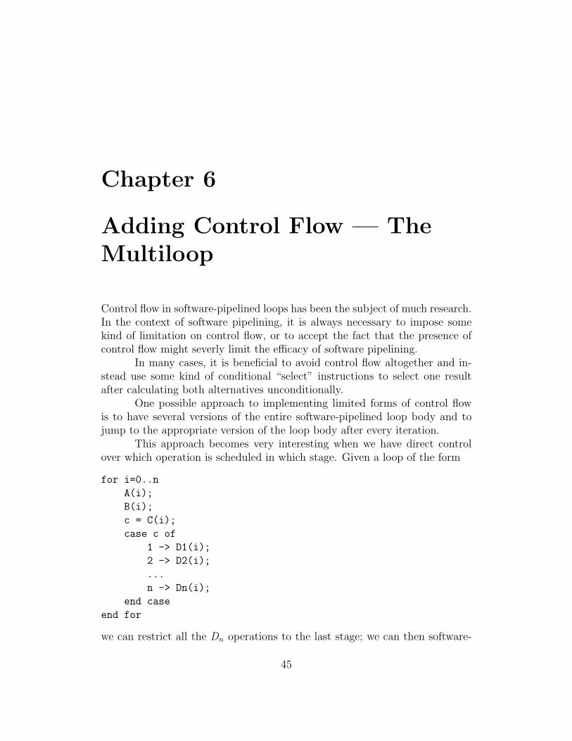
Chapter 6
Adding Control Flow — TheMultiloop
Control flow in software-pipelined loops has been the subject of much research.In the context of software pipelining, it is always necessary to impose somekind of limitation on control flow, or to accept the fact that the presence ofcontrol flow might severly limit the efficacy of software pipelining.
In many cases, it is beneficial to avoid control flow altogether and in-stead use some kind of conditional “select” instructions to select one resultafter calculating both alternatives unconditionally.
One possible approach to implementing limited forms of control flowis to have several versions of the entire software-pipelined loop body and tojump to the appropriate version of the loop body after every iteration.
This approach becomes very interesting when we have direct controlover which operation is scheduled in which stage. Given a loop of the form
for i=0..n
A(i);
B(i);
c = C(i);
case c of
1 -> D1(i);
2 -> D2(i);
...
n -> Dn(i);
end case
end for
we can restrict all the Dn operations to the last stage; we can then software-
45

M.Sc. Thesis – W. Thaller – McMaster – Computing and Software
pipeline the loop, resulting in the following structure:
A(0);
A(1); B(0);
A(2); B(1); c = C(0);
for i=0..n-3
case c of
1 -> A(i+3); B(i+2); c = C(i+1); D1(i);
...
n -> A(i+3); B(i+2); c = C(i+1); Dn(i);
end case
end for
In fact, the branch instruction at the end of the loop will be a computedbranch that will jump to the appropriate version of the loop body for the nextiteration. A branch hint instruction scheduled earlier can make this jumpalmost free of cost.
Let us now extend the definition of a loop specification from chapter 3for multiloops:
Definition 6.1 A multiloop specification with n cases is a tuple (G , n,d)containing
• a codegraph G : F ×K → F n × C
• a positive integer n
• a sequence of integers d, one for each element of F .
The control outputs C are interpreted to specify which of the n blocksof F outputs are to be used as the output of this iteration; only instructionsthat the selected set of outputs or the control outputs depend on are to beexecuted for this iteration of the loop.
Definition 6.2 We define control dependent nodes and edges in a multiloopspecification inductively:
• A node that occurs in the output sequence of G, but not at exactly thesame position(s) for all cases is control dependent.
• If a node is control dependent, then its producer is control dependent.
46

M.Sc. Thesis – W. Thaller – McMaster – Computing and Software
• If a node is control dependent, then all its consumers are control depen-dent.
• If an edge is control dependent, then all its targets are control depen-dent.
Control dependent edges are those operations which have to be differentfor different cases of the multiloop, after register allocation; if one edge in Gdelivers its result to the ith output of one case, and to the j th (i 6= j ) outputof another case, then it is control dependent, because the assembly languageinstructions in the final schedule will have to differ by their target register.
When a multiloop is software pipelined, all control dependent edgeshave to be in the last stage. For every case, a separate version of the entireloop body is scheduled. The individual versions contain the same instructionsfor stages 1 to k − 1, they only differ in the last stage.
The edges that generate the control outputs C have to be in the second-to-last stage, so that the branch instruction at the end of the loop can selectwhich version of the final stage (and therefore, which version of the scheduledloop body) to execute.
In the context of multiloops, the decision to disallow the schedulerfrom duplicating any instructions from section 2.3 pays off. For a simple loop,modulo variable expansion is always an option; in a multiloop, our scheme forhandling control flow would break down if we allowed the loop body to bereplicated.
47

M.Sc. Thesis – W. Thaller – McMaster – Computing and Software
48

Chapter 7
Experimental Results
We have implemented a prototype scheduler based on the algorithms describedin this thesis; concurrently, several efforts have been underway in our group todevelop code and other tools target the Cell SPU and the Coconut declara-tive assembly language [ACK+04], a textual representation of codegraphs. Inthe following, we give some results on how our algorithms perform on some ofthat code.
7.1 Simple Loops
We evaluate the performance of the algorithm for regular loops on a libraryof basic mathematical functions for the Cell SPU that has been developed atour work group.
Each of the basic mathematical functions takes one or two argumentsand returns one or two results; the majority take one argument and return oneresult. They operate on vectors of four floating point values in parallel. Wehave run the scheduler on loops that sequentially read input values from aninput area in memory and store the output values to a different memory area.
We can apply two different preprocessing steps to the code beforescheduling it; we can unroll the loop by replicating the loop body a u times inparallel (the parallel instances of the loop body will use common loop countinginstructions).
We can also apply a preprocessing step that splits up the m nodeswith the greatest lifetimes (as estimated before scheduling using the heightLU
function from section 4.1) by inserting register-to-register move instructions(we use the rotqbyi 0 instruction, rotate quad word by zero bytes).
Tables 7.1 and 7.2 show the result of applying the heuristic staging
49

M.Sc. Thesis – W. Thaller – McMaster – Computing and Software
u = 1 u = 2s m b n r s m b n r
acos 6 2 28 43 38 6 4 55 59 58acosh 5 2 23 32 37 5 4 45 45 49
asin 6 2 28 54 39 4 4 55 77 44asinh 5 2 21 35 36 5 4 41 42 46atan2 2 2 24 103 32 2 4 47 103 43atanh 7 2 20 21 40 3 0 39 42 41
cbrt 3 2 21 26 39 3 4 41 44 41cos 4 2 26 29 41 4 4 51 51 53
cosh 6 2 17 28 36 6 4 33 34 44div 2 2 13 24 13 2 4 17 20 17exp 4 0 13 23 29 4 4 23 25 36
log10 5 2 15 23 35 6 4 25 25 48log 5 2 15 23 35 6 4 25 25 48
pow 5 2 23 41 45 4 4 45 46 58qdrt 5 2 13 25 17 4 4 25 40 23rcbrt 5 2 24 32 40 5 4 47 49 56
rec 4 2 11 15 13 3 4 14 19 14rqdrt 4 2 12 21 17 4 4 19 26 24rsqrt 4 2 11 19 15 2 4 14 23 18
sin 4 2 26 30 43 3 4 51 51 50sincos 5 2 29 32 50 3 0 57 57 51
sinh 6 2 17 28 36 6 4 33 34 44sqrt 4 2 11 23 15 3 4 14 20 18tan 5 2 33 40 45 2 4 65 65 47
tanh 8 2 19 25 37 6 4 37 37 46
Table 7.1: Results of scheduling math functions in simple loops for unrollingfactors 1 (no unrolling) and 2
algorithm followed by a simple list-scheduling algorithm to schedule the trans-formed loop body; for each function and each value of the unrolling factoru, the table shows the number of stages s and the number of inserted movesm that yielded the shortest schedule; for this shortest schedule, it shows the
50

M.Sc. Thesis – W. Thaller – McMaster – Computing and Software
u = 3 u = 4s m b n r s m b n r
acos 5 0 82 87 59 3 0 109 112 69acosh 3 6 67 69 51 2 0 89 91 56
asin 3 6 82 91 61 3 8 109 110 76asinh 3 6 61 61 51 3 8 81 81 62atan2 2 6 70 105 52 2 8 93 107 60atanh 3 0 58 59 51 3 8 77 77 61
cbrt 2 6 61 61 51 2 8 81 81 60cos 3 6 76 79 58 3 8 101 102 70
cosh 6 6 49 49 56 4 0 65 65 61div 2 6 21 23 21 2 0 23 24 22exp 4 6 34 34 44 4 8 45 45 52
log10 3 6 37 37 42 3 8 49 49 48log 3 6 37 37 42 3 8 49 49 48
pow 3 6 67 67 63 3 8 89 90 74qdrt 4 6 37 50 30 2 8 49 59 34rcbrt 4 6 70 70 65 4 8 93 93 78
rec 2 6 17 19 17 2 8 20 21 20rqdrt 3 6 28 37 28 3 8 37 44 34rsqrt 2 6 17 23 22 2 0 21 24 25
sin 3 0 76 76 59 3 8 101 101 72sincos 3 6 85 85 63 2 8 113 113 66
sinh 6 6 49 49 56 4 0 65 65 61sqrt 3 6 19 37 22 2 8 25 37 26tan 2 0 97 97 57 2 8 129 129 63
tanh 5 6 55 55 54 6 8 73 73 74
Table 7.2: Results of scheduling math functions in simple loops for unrollingfactors 3 and 4
theoretical lower bound b for the schedule length calculated from the numberof instructions for each of the Cell SPU’s two execution units, the achievedschedule length (in cycles) n and the number of registers r used by the sched-ule.
As was to be expected, we can see that we are more likely to find a
51

M.Sc. Thesis – W. Thaller – McMaster – Computing and Software
u = 1 u = 2s m b n nm ∆ s m b n nm ∆
acos 3 2 28 54 54 0 3 4 55 63 64 1acosh 3 2 23 44 44 0 3 4 45 50 51 1
asin 3 2 28 77 78 1 3 4 55 82 93 11asinh 3 2 21 51 54 3 3 4 41 50 54 4atanh 3 0 20 41 42 1 3 0 39 42 44 2
cbrt 3 2 21 26 31 5 3 4 41 44 44 0cos 2 2 26 39 41 2 3 0 51 52 55 3
cosh 3 2 17 43 45 2 3 4 33 43 48 5div 3 2 13 24 32 8 2 4 17 20 29 9exp 2 2 15 31 31 0 3 4 23 31 39 8
log10 3 2 15 29 27 -2 3 4 25 26 30 4log 3 2 15 29 27 -2 3 4 25 26 30 4
pow 3 2 23 48 53 5 3 4 45 51 57 6qdrt 3 2 13 34 36 2 3 4 25 43 43 0rcbrt 3 2 24 39 38 -1 3 4 47 55 55 0
rec 3 2 11 18 25 7 3 4 14 19 32 13rqdrt 3 2 12 36 38 2 3 4 19 37 36 -1rsqrt 3 2 11 21 22 1 2 4 14 23 24 1
sin 3 2 26 36 50 14 3 4 51 51 57 6sincos 3 2 29 38 47 9 3 0 57 57 63 6
sinh 3 2 17 43 45 2 3 4 33 43 48 5sqrt 3 2 11 24 26 2 3 4 14 20 28 8tan 3 2 33 51 53 2 2 4 65 65 69 4
tanh 3 2 19 52 52 0 3 4 37 54 54 0
Table 7.3: Merge Scheduling vs. List Scheduling, unrolling factors 1 and 2
schedule close to the minimum bound at higher unrolling factors; we have goodschedules for u = 1 for a few of the functions (atanh, cos, sin, sincos); at u = 2,we have reason to be happy with most of the schedules, and for u = 4, almostall functions schedule within a few cycles of the theoretical lower bound b.
Merge scheduling, while having polynomial complexity in the size ofits input, is exponential in the number of stages; For the math functions
52
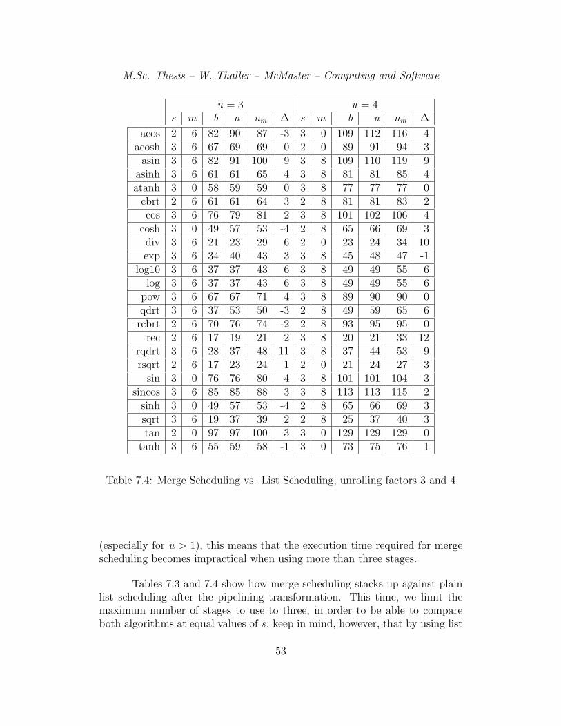
M.Sc. Thesis – W. Thaller – McMaster – Computing and Software
u = 3 u = 4s m b n nm ∆ s m b n nm ∆
acos 2 6 82 90 87 -3 3 0 109 112 116 4acosh 3 6 67 69 69 0 2 0 89 91 94 3
asin 3 6 82 91 100 9 3 8 109 110 119 9asinh 3 6 61 61 65 4 3 8 81 81 85 4atanh 3 0 58 59 59 0 3 8 77 77 77 0
cbrt 2 6 61 61 64 3 2 8 81 81 83 2cos 3 6 76 79 81 2 3 8 101 102 106 4
cosh 3 0 49 57 53 -4 2 8 65 66 69 3div 3 6 21 23 29 6 2 0 23 24 34 10exp 3 6 34 40 43 3 3 8 45 48 47 -1
log10 3 6 37 37 43 6 3 8 49 49 55 6log 3 6 37 37 43 6 3 8 49 49 55 6
pow 3 6 67 67 71 4 3 8 89 90 90 0qdrt 3 6 37 53 50 -3 2 8 49 59 65 6rcbrt 2 6 70 76 74 -2 2 8 93 95 95 0
rec 2 6 17 19 21 2 3 8 20 21 33 12rqdrt 3 6 28 37 48 11 3 8 37 44 53 9rsqrt 2 6 17 23 24 1 2 0 21 24 27 3
sin 3 0 76 76 80 4 3 8 101 101 104 3sincos 3 6 85 85 88 3 3 8 113 113 115 2
sinh 3 0 49 57 53 -4 2 8 65 66 69 3sqrt 3 6 19 37 39 2 2 8 25 37 40 3tan 2 0 97 97 100 3 3 0 129 129 129 0
tanh 3 6 55 59 58 -1 3 0 73 75 76 1
Table 7.4: Merge Scheduling vs. List Scheduling, unrolling factors 3 and 4
(especially for u > 1), this means that the execution time required for mergescheduling becomes impractical when using more than three stages.
Tables 7.3 and 7.4 show how merge scheduling stacks up against plainlist scheduling after the pipelining transformation. This time, we limit themaximum number of stages to use to three, in order to be able to compareboth algorithms at equal values of s ; keep in mind, however, that by using list
53

M.Sc. Thesis – W. Thaller – McMaster – Computing and Software
scheduling directly, we can use higher values for s and thereby achieve betterschedules in many cases.
In addition to the columns we have seen in the earlier tables, thesetables show the schedule length nm achieved by merge scheduling and the dif-ference ∆ = nm−n between the schedule lengths achieved by merge schedulingand list scheduling. The tables do not show register usage.
The difference ∆ varies from −4 to 14; in most cases, the simpler al-gorithm, list scheduling, is also the better one. In those cases where mergescheduling delivers a better schedule, it does so by only a few cycles; it is con-ceivable that minor adjustments to the priority function used in list schedulingmight allow list scheduling to catch up there, too.
If we take into account the high time complexity of merge scheduling,we unfortunately have to conclude that merge scheduling is not suitable forpractical use.
7.2 Multiloop
We have developed one real-world algorithm that exploits the strengths of themultiloop to the fullest. The algorithm was initially developed by Dr. Anandand not only serves as a test case for the multiloop scheduler, but also servedas the original inspiration for the concept of a multiloop.
As part of a non-uniform fourier transform, we need to resample non-uniform samples in three-dimensional space to a regular grid; more specifically,we have samples along a trajectory through three-dimensional space, and weneed to convolve these samples with a gaussian kernel. It boils down to havingto add something to the entries near the position of the sample in the three-dimensional grid, for every sample on the trajectory.
The distance between two successive samples is small, so that many ofthe same grid positions will be affected by two consecutive samples; in fact,it is guaranteed to be less than the size of a grid cell per dimension. Wetherefore have a window of interest that moves by at most one grid cell inevery dimension for each sample in the input.
At 128 registers, the Cell SPU’s register file is large enough to accomo-date a decently-sized window of 4× 4× 4 complex values, stored in 32 vectorregisters.
The loop will, at each step, add the kernel to the current window (whichis in registers) and then, depending on the trajectory, move the window bystoring “old” values, shifting all values in the window, and loading “new”values. The 33 = 27 different possible directions to move the window (including
54

M.Sc. Thesis – W. Thaller – McMaster – Computing and Software
the case of not moving at all) are each implemented as a case of the multiloop.Things are further complicated by the fact that the Cell SPU only
supports vector-aligned loads and stores; we therefore need to round up thesize of the register window in the unaligned case; we keep the “unused” partsof the unaligned window in 4× 4 additional registers. Adding the convolutionkernel to the register window works the same for both aligned and unalignedwindows; the extra registers are not modified. Moving the window, however,needs to be done differently for the aligned and for the unaligned case. Thisdoubles the total number of different cases to 54.
Tables 7.5 and 7.6 show the results of scheduling the multiloop; foreach of the 54 cases, the table shows the lower bound b, the length n of theschedule achieved by heuristic staging followed by list scheduling, the numberr of registers used, the length nm of the schedule achieved by heuristic stagingfollowed by merge scheduling, and the difference nm − n between the resultsof the two scheduling strategies.
Merge scheduling is again outperformed on most cases, and it evenhappens to deliver one of its worst results on case 53, which will be executedmost often, as it is the case where the register window does not move.
On the other hand, we see that by software pipelining the multiloopusing our heuristic staging algorithm, we can achieve close-to-optimal sched-ules for most of the 54 cases of our code; we are confident that this level ofperformance cannot be reached without using a software-pipelined multiloop.
55

M.Sc. Thesis – W. Thaller – McMaster – Computing and Software
# b n r nm nm − n
0 151 151 110 151 01 151 156 92 159 32 151 152 110 151 -13 151 155 92 159 44 87 98 87 98 05 143 143 110 143 06 151 151 110 151 07 151 156 91 159 38 151 154 110 151 -39 151 156 92 159 3
10 87 104 88 103 -111 143 145 110 143 -212 139 141 108 139 -213 139 144 92 150 614 139 139 108 139 015 139 144 91 150 616 81 91 85 100 917 107 117 104 117 018 151 151 110 151 019 151 156 92 159 320 151 151 110 151 021 151 156 92 159 322 87 103 88 103 023 143 143 110 143 024 151 151 109 151 025 151 155 91 159 426 151 151 109 151 0
Table 7.5: Scheduling results for the 3D resampling multiloop, cases 0 through26
56

M.Sc. Thesis – W. Thaller – McMaster – Computing and Software
# b n r nm nm − n
27 151 155 92 159 428 87 101 87 102 129 143 143 110 143 030 139 139 107 139 031 139 144 90 150 632 139 139 107 139 033 139 144 91 150 634 81 91 83 100 935 107 117 102 117 036 139 139 109 139 037 139 144 92 151 738 139 139 108 139 039 139 144 91 151 740 80 97 88 101 441 107 115 110 115 042 139 139 108 139 043 139 144 92 151 744 139 139 107 139 045 139 144 92 151 746 80 99 87 99 047 107 120 108 114 -648 123 125 111 130 549 123 127 93 141 1450 123 123 111 130 751 123 127 93 141 1452 80 86 86 99 1353 79 86 86 99 13
Table 7.6: Scheduling results for the 3D resampling multiloop, cases 27 through53
57

M.Sc. Thesis – W. Thaller – McMaster – Computing and Software
58

Chapter 8
Conclusions & Outlook
We have developed a new method of software pipelining that gives explicitcontrol about which stages operations are assigned to.
We have defined a way of describing loops that allows specifying arbi-trary inter-iteration dataflow, allowing the user or earlier stages in the com-pilation process to take better advantage of software pipelining. We haveformalised software pipelining as a transformation between such loop specifi-cations.
Controlling stage assignment explicitly and avoiding the need for mod-ulo variable expansion after scheduling allowed us to handle a special but veryuseful case of control flow, the multiloop very efficiently. Even though severaldesign decisions were made specifically to support the multiloop, the algorithmalso performs well on a selection of simple loops.
As a future research direction, it should be investigated whether theheuristics of decomposed software pipelining [WEJS94; GS94; CDR98], espe-cially the circuit-retiming based approach given in [CDR98], can be adapted toour framework. The algorithm of [CDR98] has a known efficiency bound, butit does not currently have any provisions for pre-assigning stages (required forthe multiloop). Also, it does not limit the lifetime of values to λ, but insteadrelies on modulo variable expansion to handle these long lifetimes, which againprecludes its use for scheduling multiloops.
In [KAC06], the concept of joins is discussed; the idea is to allow a nodein the codegraph to have multiple producers; the scheduler is then expected tochoose one alternative, based on which leads to the better code. This wouldallow us to specify a loop like the one from figure 2.3 (section 2.5) withouthaving to decide on a value for the iteration distance x before scheduling;instead, the loop specification would contain a join that tells the scheduler tochoose among several inputs with different d values.
59

M.Sc. Thesis – W. Thaller – McMaster – Computing and Software
60

Bibliography
[ACK+04] Christopher Kumar Anand, Jacques Carette, Wolfram Kahl, CaleGibbard, and Ryan Lortie. Declarative assembler. SQRL Re-port 20, Software Quality Research Laboratory, McMaster Uni-versity, October 2004. available from http://sqrl.mcmaster.ca/
sqrl reports.html.
[AJLA95] Vicki H. Allan, Reese B. Jones, Randall M. Lee, and Stephen J.Allan. Software pipelining. ACM Computing Surveys, 27(3):367–432, 1995.
[CDR98] P.-Y. Calland, A. Darte, and Y. Robert. Circuit retiming appliedto decomposed software pipelining. IEEE Transactions on Paralleland Distributed Systems, 9(1):24–35, 1998.
[GS94] Franco Gasperoni and Uwe Schwiegelshohn. Generating close tooptimum loop schedules on parallel processors. Parallel ProcessingLetters, 4:391–403, 1994.
[IBM06] IBM Corp, Sony Inc. and Toshiba Corp. Cell Broadband EngineProgramming Handbook, 2006.
[KAC06] Wolfram Kahl, Christopher Kumar Anand, and Jacques Carette.Control-flow semantics for assembly-level data-flow graphs. InWendy McCaull, Michael Winter, and Ivo Duntsch, editors,8th Intl. Seminar on Relational Methods in Computer Science,RelMiCS 8, Feb. 2005, volume 3929 of LNCS, pages 147–160.Springer-Verlag, 2006.
[Lam88] M. Lam. Software pipelining: an effective scheduling technique forVLIW machines. SIGPLAN Not., 23(7):318–328, 1988.
[RG81] B. R. Rau and C. D. Glaeser. Some scheduling techniques andan easily schedulable horizontal architecture for high performance
61

M.Sc. Thesis – W. Thaller – McMaster – Computing and Software
scientific computing. In MICRO 14: Proceedings of the 14th annualworkshop on Microprogramming, pages 183–198, Piscataway, NJ,USA, 1981. IEEE Press.
[RGSL96] John Ruttenberg, G. R. Gao, A. Stoutchinin, and W. Lichtenstein.Software pipelining showdown: optimal vs. heuristic methods in aproduction compiler. In PLDI ’96: Proceedings of the ACM SIG-PLAN 1996 conference on Programming language design and im-plementation, pages 1–11, New York, NY, USA, 1996. ACM Press.
[RST92] B. Ramakrishna Rau, Michael S. Schlansker, and P. P. Tirumalai.Code generation schema for modulo scheduled loops. SIGMICRONewsl., 23(1-2):158–169, 1992.
[RYYT89] B.R. Rau, D.W.L. Yen, W. Yen, and R.A. Towle. The Cydra 5departmental supercomputer: design philosophies, decisions andtrade-offs. In System Sciences, 1989. Vol.I: Architecture Track,Proceedings of the Twenty-Second Annual Hawaii InternationalConference on, volume 1, pages 202–213, Kailua-Kona, HI, USA,1989.
[WEJS94] Jian Wang, Christine Eisenbeis, Martin Jourdan, and Bogong Su.Decomposed software pipelining: a new perspective and a new ap-proach. Int. J. Parallel Program., 22(3):351–373, 1994.
62