exploiting consistency among heterogeneous …...exploits the natural redundancy amongst...

AbstractModern vehicles house many advanced components; sensors and Electronic Control Units (ECUs) — now numbering in the 100s. These components provide various advanced safety, comfort and infotainment features, but they also introduce additional attack vectors for malicious entities. Attackers can compromise one or more of these sensors and flood the vehicle’s internal network with fake sensor values. Falsified sensor values can confuse the driver, and even cause the vehicle to misbehave. Redundancy can be used to address compromised sensors, but adding redundant sensors will increase the cost per vehicle and is therefore less attractive.

To balance the need for security and cost-efficiency, we exploit the natural redundancy found in vehicles. Natural redundancy occurs when the same physical phenomenon causes symptoms in multiple sensors. For instance, pressing the accelerator pedal will cause the engine to pump faster and increase the speed of the vehicle. Engine RPM and vehicle speed are multiple sensors which respond in a related fashion to the same cause of the accelerator pedal. The challenge is identifying the relationship between similar but different sensors under normal operation and detecting anomalous be-havior accurately.

In this paper, we develop the tools to capture the relationship between sensors. Specifically, we use the pairwise correlation between key variables, and use cluster-analysis to identify distinct behavior of drivers. Moreover, we show preliminary results of using these tools to detect attacks within a vehicular communication bus.

Keywordssensing redundancy, cyber-physical security, anomaly detection

1. IntroductionA modern vehicle is a complex system with many interconnected Electronic Control Units (ECUs). These ECUs broadcast sensor measurements and control information onto a shared communication channel, often a Controller Area Network (CAN) bus. The vehicle performs various actions by aggregating sensor information from multiple ECUs. For example, the Intelligent Park Assist System (IPAS) in the Toyota Prius 2010 model activates only when the car is in reverse gear and traveling less than 4 mph [8]. However, attackers can spoof values in the CAN bus to cause the vehicle to behave incorrectly or maliciously. Miller and Valasek [8] demonstrate this by sending fake speedometer and gear position values on the CAN bus to trigger the IPAS and cause sporadic jumps in the steering wheel even when the car is moving.

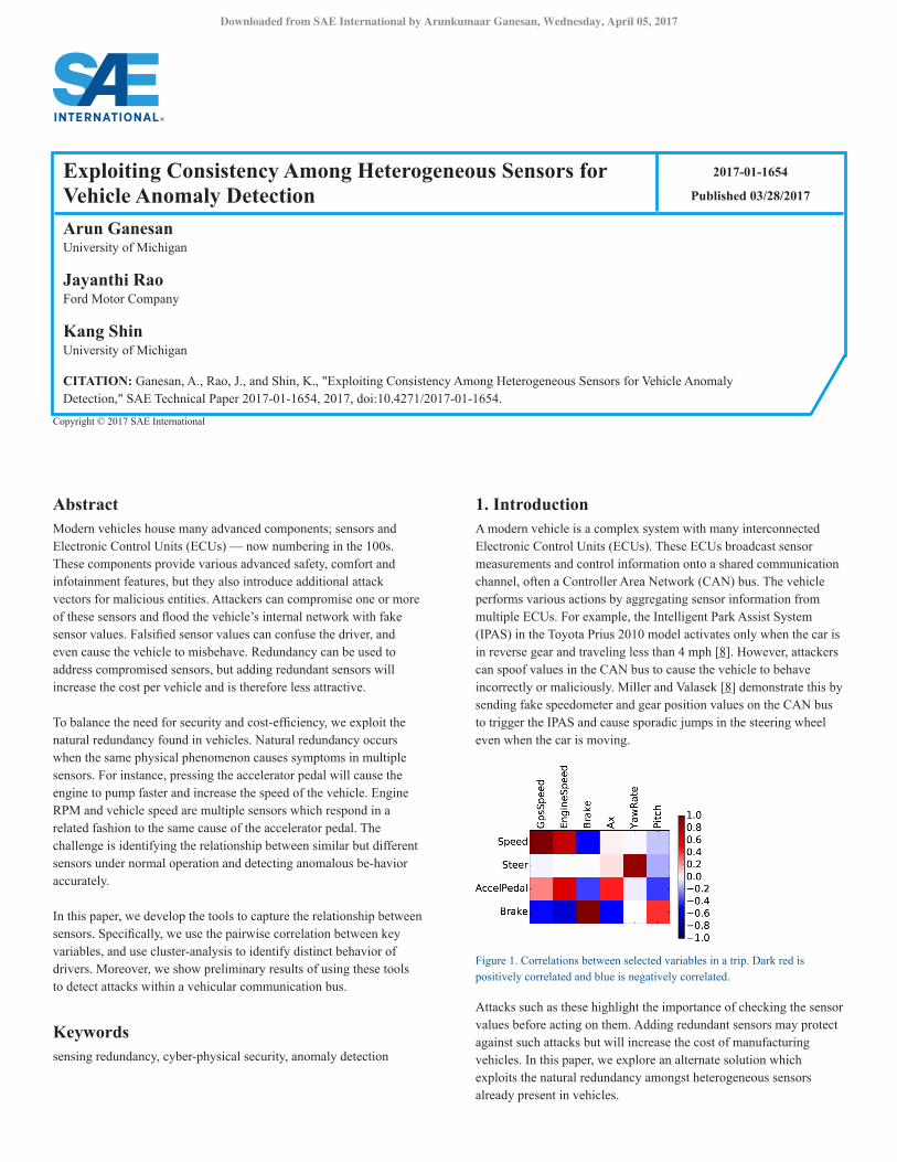
Figure 1. Correlations between selected variables in a trip. Dark red is positively correlated and blue is negatively correlated.

Attacks such as these highlight the importance of checking the sensor values before acting on them. Adding redundant sensors may protect against such attacks but will increase the cost of manufacturing vehicles. In this paper, we explore an alternate solution which exploits the natural redundancy amongst heterogeneous sensors already present in vehicles.

Exploiting Consistency Among Heterogeneous Sensors for Vehicle Anomaly Detection

2017-01-1654

Published 03/28/2017

Arun GanesanUniversity of Michigan

Jayanthi RaoFord Motor Company

Kang ShinUniversity of Michigan

CITATION: Ganesan, A., Rao, J., and Shin, K., "Exploiting Consistency Among Heterogeneous Sensors for Vehicle Anomaly Detection," SAE Technical Paper 2017-01-1654, 2017, doi:10.4271/2017-01-1654.

Copyright © 2017 SAE International

Downloaded from SAE International by Arunkumaar Ganesan, Wednesday, April 05, 2017

We begin with the observation that sensors within the vehicle are naturally correlated. This happens because the same physical phenomenon creates effects in multiple sensors. For example, turning the steering wheel causes an increase in the yaw-rate. We show some example correlations from our experiments in Fig. 1.

In this paper, we study the persistence of these correlations within a trip, across trips, across drivers and across vehicles. Armed with an understanding of these correlations, we develop tools to detect attacks or system faults which cause anomalous correlations between pairs of sensors.

Our experiments are based on the Integrated Vehicle-Based Safety Systems (IVBSS) dataset collected by the University of Michigan Transportation Research Institute [4]. IVBSS contains naturalistic driving behavior of 108 drivers for 16 cars between April 2009 – May 2010.

Our evaluation shows that some pairs of variables are consistently correlated across trips, drivers and vehicles. However, we found large variation for small time windows (e.g. 100 seconds) within a trip. This variability is caused by contextual factors of the driver and trip. We use cluster analysis for quantitatively identifying contextual factors and measuring their impact on the variability of pairwise clusters.

We make the following three main contributions.

• Analysis of pairwise correlation of vehicular sensors. Our analysis revealed insights into pairwise correlation which can be used for future research. We exploit the natural redundancy found in vehicular sensors.

• Application of cluster-analysis to identify contexts of vehicular data. This step is crucial in reducing the intra-trip variation found in pairwise correlation.

• Preliminary assessment of pairwise correlation analysis in malicious data injection attack detection.

This paper is organized as follows. We review related work and motivate our approach in Sec. 2. Sec. 3 describes the IVBSS dataset and introduces our core analytic approach — the correlation matrix. In Sec. 4, we explore the macroscopic persistence of pairwise correlations across trips, drivers and vehicles, while in Sec. 5, we investigate the microscopic variability of pairwise correlations within a trip. In Sec. 6, we use our understanding of pairwise correlation to develop an intrusion or fault detection method. Finally, we discuss limitations and future work in Sec. 7 and conclude the paper in Sec. 8.

2. Related WorkVehicle infrastructure has recently been under the scrutiny of security researchers. Koscher et al.[6] demonstrated a wide range of vehicular attacks that are enabled once the attacker gains access to the internal CAN bus. Some of the reported attacks may have significant safety-critical effects such as disabling the brakes or killing the engine. In a follow-up to this work, Checkoway et al.[1] demonstrated that such attacks were possible even without direct

physical access to the victim’s vehicle. Such vehicular attacks were reproduced by other researchers [5, 8] leading to an increase in mass public attention for vehicular security.

There are many proposed solutions to detect and defend against these attacks. Among these, proposals which compare and validate cross-sensory data are the most relevant to our approach. Cho et al.[2] detect anomalies in the brake sub-system by modeling vehicle dynamics. They use the tire friction and current road condition to model the expected braking behavior. In contrast to their work, our solution is more general and does not require carefully tuned models for each sub-system. Our system finds correlations between sensors in a data-driven fashion.

Liu et al.[7] detect anomalies in cyber-physical systems using a spatiotemporal pattern network and a restricted Boltzman machine. They demonstrate how their technique can detect anomalies in smart home monitoring environments. In contrast with this domain, vehicular sensors naturally express large variations, many of which may be falsely considered as anomalous. Our approach reduces the large variation by identifying the current context of the data. By considering contextual variables, our solution is likely to yield a more accurate attack detection rate in diverse situations.

Table 1. IVBSS data sources used in our experiments.

Pajic et al.[9] develop an attack-resilient state estimator which functions in the presence of sensor noise. They demonstrate this on an automatic cruise-control for a ground vehicle. Their system requires a model of how components interact. In a vehicular context, this is hard to devise due to many factors outside of our control. Our approach attempts to automatically derive the relationships between variables in the vehicle without any prior vehicular model.

3. Analysis OverviewHere we describe the IVBSS dataset used in all our experiments and describe pairwise correlation of sensors — the main technique used in our analysis.


3.1. IVBSS DatasetThe Integrated Vehicle-based Safety System (IVBSS) dataset [4] was collected between April 2009 and May 2010 by the University of Michigan Transportation Research Institute (UMTRI) to evaluate the impact of collision avoidance systems in driver behavior. The researchers recruited 108 drivers in Michigan and distributed 16 Honda Accords (2006 and 2007 models) amongst them for 6 weeks at a time. During this time, they collected diverse sensor data from within the vehicle and from the collision avoidance systems. The data was collected at various data rates and resampled and normalized to 10Hz. A selection of some of the variables is shown in Table 1. In total, the IVBSS dataset contains over 213,000 miles of driving.

3.2. Pairwise CorrelationAt the heart of our analysis is pairwise correlation of variables. We study pairwise correlation in the short-time scale — within trips — and the larger time scale — across trips, drivers, and vehicles. Normal behavior causes related change within the vehicle. For instance, pressing the accelerator pedal will result in an increase in the speed of the car, cause acceleration in the forward direction, an increase in the engine RPM, and a gear shift for automatic systems. However, in the presence of a fault or an attack, these relationships will no longer hold. If an attacker spoofs the speed of the vehicle, that will no longer correlate with the accelerator pedal behavior, and therefore can be identified as anomalous.

We performed pairwise correlation between all variables from Table 1. The variables are divided into two classes — sensors within the vehicle which are broadcast on the CAN bus, and sensors from an external IMU/GPS system. Correlating both internal and external sensors gives us additional redundancy and robustness of the system. In order to successfully fool the system, the attacker has to compromise both internal and external systems, thus increasing the difficulty for a successful attack.

Based on the pairwise correlation matrix, we found unexpected and interesting correlations of sensors for individual trips. In many trips, the pitch of the vehicle is positively correlated with the acceleration pedal negatively correlated with the brake pedal. This captures when the vehicle slightly dips forward or backward when the driver depresses the acceleration pedal. We also found that the steering wheel angle is positively correlated with the yaw rate and that the brake is negatively correlated with many variables such as speed, throttle, engine speed and acceleration.

However, these correlations differ across multiple trips. To study this systematically, we explore which variables are consistently correlated for the same driver and how this changes across different drivers and different cars. This is presented in the next section.

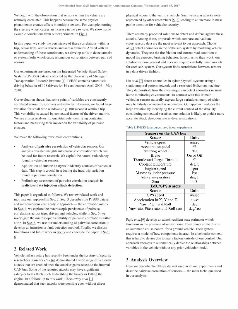
4. Across-trip ConsistencyThe pairwise correlation of sensors often changes between trips and between drivers. Fig. 2 shows the correlation and average change of the correlation across all trips for a single driver. From all pairs of variables, we identified 14 pairs which have greater than 0.5 correlation across for at least one driver. The top sensors and the corresponding average correlation matrix are shown in the bottom row of Fig. 2 and listed in Table 2.

Among the highly correlated variables, we found four pairs to be nearly 100% positively correlated in nearly all the trips. These four were speed and GPS speed, acceleration pedal and target throttle, throttle and target throttle, and acceleration pedal and target throttle. The vehicles in our dataset broadcast the target throttle and current throttle as separate values. Due to their high correlation, we can easily detect if an attacker modifies one of the variables and not the other.

In order to use the bounds for attack detection, we must use a model of the correlations that best resembles each driver. The correlations shown in Table 2 are for one driver. For a single driver, we calculated the correlation of the sensors for a each trip, and measured how much it changed from one trip to the next. We show the average correlation across trips and the average change in the top right of Fig. 2. In the bottom right, we show the same values for the pairs specified in Table. 2.

Table 2. Highly correlated pairs, their average correlation and their average change in correlation across trips for a single driver. Results were similar for other drivers and are thus omitted.

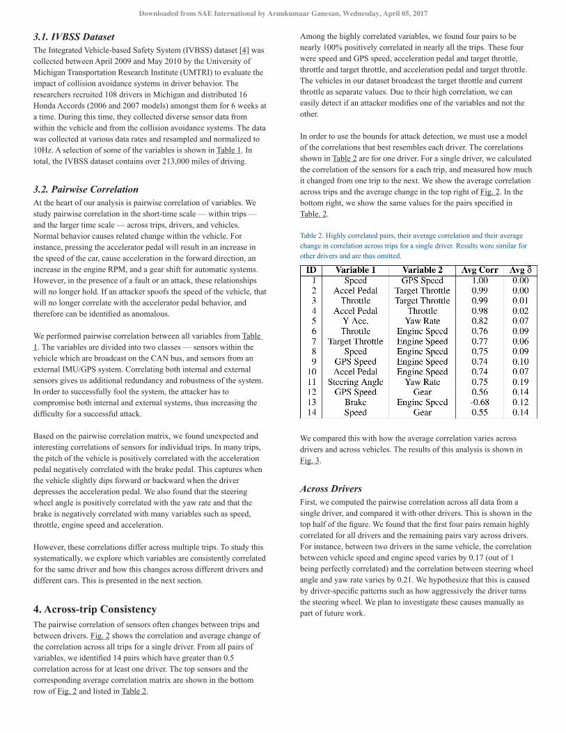
We compared this with how the average correlation varies across drivers and across vehicles. The results of this analysis is shown in Fig. 3.

Across DriversFirst, we computed the pairwise correlation across all data from a single driver, and compared it with other drivers. This is shown in the top half of the figure. We found that the first four pairs remain highly correlated for all drivers and the remaining pairs vary across drivers. For instance, between two drivers in the same vehicle, the correlation between vehicle speed and engine speed varies by 0.17 (out of 1 being perfectly correlated) and the correlation between steering wheel angle and yaw rate varies by 0.21. We hypothesize that this is caused by driver-specific patterns such as how aggressively the driver turns the steering wheel. We plan to investigate these causes manually as part of future work.


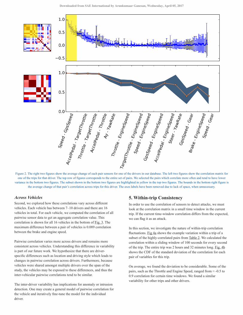
Figure 2. The right two figures show the average change of each pair sensors for one of the drivers in our database. The left two figures show the correlation matrix for one of the trips for that driver. The top row of figures corresponds to the entire set of pairs. We selected the pairs which correlate more often and tend to have lower

variance in the bottom two figures. The subset shown in the bottom two figures are highlighted in yellow in the top two figures. The bounds in the bottom right figure is the average change of that pair’s correlation across trips for this driver. The axes labels have been removed due to lack of space, when unnecessary.

Across VehiclesSecond, we explored how these correlations vary across different vehicles. Each vehicle has between 7–10 drivers and there are 16 vehicles in total. For each vehicle, we computed the correlation of all pairwise sensor data to get an aggregate correlation value. This correlation is shown for all 16 vehicles in the bottom of Fig. 3. The maximum difference between a pair of vehicles is 0.089 correlation between the brake and engine speed.

Pairwise correlation varies more across drivers and remains more consistent across vehicles. Understanding this difference in variability is part of our future work. We hypothesize that there are driver-specific differences such as location and driving style which leads to changes in pairwise correlation across drivers. Furthermore, because vehicles were shared amongst multiple drivers over the span of the study, the vehicles may be exposed to these differences, and thus the inter-vehicular pairwise correlations tend to be similar.

The inter-driver variability has implications for anomaly or intrusion detection. One may create a general model of pairwise correlation for the vehicle and iteratively fine-tune the model for the individual driver.

5. Within-trip ConsistencyIn order to use the correlation of sensors to detect attacks, we must look at the correlation matrix in a small time window in the current trip. If the current time-window correlation differs from the expected, we can flag it as an attack.

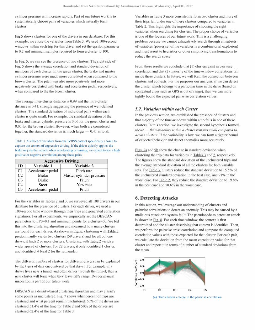
In this section, we investigate the nature of within-trip correlation fluctuations. Fig 4a shows the example variation within a trip of a subset of the highly-correlated pairs from Table 2. We calculated the correlation within a sliding window of 100 seconds for every second of the trip. The entire trip was 2 hours and 32 minutes long. Fig. 4b shows the CDF of the standard deviation of the correlation for each pair of variables for this trip.

On average, we found the deviation to be considerable. Some of the pairs, such as the Throttle and Engine Speed, ranged from ≈ -0.5 to 0.9 correlation for certain time windows. We found a similar variability for other trips and other drivers.


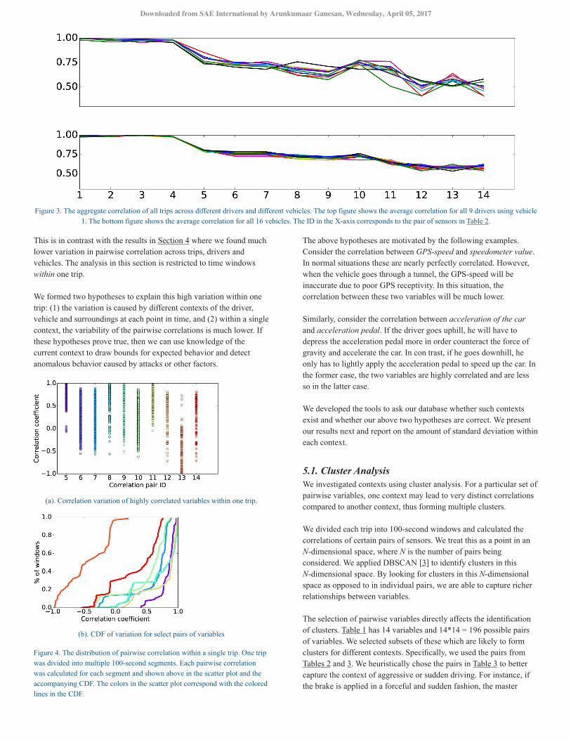
Figure 3. The aggregate correlation of all trips across different drivers and different vehicles. The top figure shows the average correlation for all 9 drivers using vehicle 1. The bottom figure shows the average correlation for all 16 vehicles. The ID in the X-axis corresponds to the pair of sensors in Table 2.

This is in contrast with the results in Section 4 where we found much lower variation in pairwise correlation across trips, drivers and vehicles. The analysis in this section is restricted to time windows within one trip.

We formed two hypotheses to explain this high variation within one trip: (1) the variation is caused by different contexts of the driver, vehicle and surroundings at each point in time, and (2) within a single context, the variability of the pairwise correlations is much lower. If these hypotheses prove true, then we can use knowledge of the current context to draw bounds for expected behavior and detect anomalous behavior caused by attacks or other factors.

(a). Correlation variation of highly correlated variables within one trip.

(b). CDF of variation for select pairs of variables

Figure 4. The distribution of pairwise correlation within a single trip. One trip was divided into multiple 100-second segments. Each pairwise correlation was calculated for each segment and shown above in the scatter plot and the accompanying CDF. The colors in the scatter plot correspond with the colored lines in the CDF.

The above hypotheses are motivated by the following examples. Consider the correlation between GPS-speed and speedometer value. In normal situations these are nearly perfectly correlated. However, when the vehicle goes through a tunnel, the GPS-speed will be inaccurate due to poor GPS receptivity. In this situation, the correlation between these two variables will be much lower.

Similarly, consider the correlation between acceleration of the car and acceleration pedal. If the driver goes uphill, he will have to depress the acceleration pedal more in order counteract the force of gravity and accelerate the car. In con trast, if he goes downhill, he only has to lightly apply the acceleration pedal to speed up the car. In the former case, the two variables are highly correlated and are less so in the latter case.

We developed the tools to ask our database whether such contexts exist and whether our above two hypotheses are correct. We present our results next and report on the amount of standard deviation within each context.

5.1. Cluster AnalysisWe investigated contexts using cluster analysis. For a particular set of pairwise variables, one context may lead to very distinct correlations compared to another context, thus forming multiple clusters.

We divided each trip into 100-second windows and calculated the correlations of certain pairs of sensors. We treat this as a point in an N-dimensional space, where N is the number of pairs being considered. We applied DBSCAN [3] to identify clusters in this N-dimensional space. By looking for clusters in this N-dimensional space as opposed to in individual pairs, we are able to capture richer relationships between variables.

The selection of pairwise variables directly affects the identification of clusters. Table 1 has 14 variables and 14*14 = 196 possible pairs of variables. We selected subsets of these which are likely to form clusters for different contexts. Specifically, we used the pairs from Tables 2 and 3. We heuristically chose the pairs in Table 3 to better capture the context of aggressive or sudden driving. For instance, if the brake is applied in a forceful and sudden fashion, the master


cylinder pressure will increase rapidly. Part of our future work is to systematically choose pairs of variables which naturally form clusters.

Fig 5 shows clusters for one of the drivers in our database. For this example, we chose the variables from Table 3. We used 100-second windows within each trip for this driver and set the epsilon parameter to 0.2 and minimum samples required to form a cluster to 100.

In Fig. 5, we can see the presence of two clusters. The right side of Fig. 5 shows the average correlation and standard deviation of members of each cluster. In the green cluster, the brake and master cylinder pressure were much more correlated when compared to the brown cluster. The pitch was also more positively and more negatively correlated with brake and accelerator pedal, respectively, when compared to the the brown cluster.

The average inter-cluster distance is 0.99 and the intra-cluster distance is 0.41, strongly suggesting the presence of well-defined clusters. The standard deviation of individual pairs within each cluster is quite small. For example, the standard deviation of the brake and master cylinder pressure is 0.06 for the green cluster and 0.05 for the brown cluster. However, when both are considered together, the standard deviation is much larger — 0.41 in total.

Table 3. A subset of variables from the IVBSS dataset specifically chosen to capture the context of aggressive driving. If the driver quickly applies the brake or jolts the vehicle when accelerating or turning, we expect to see a high positive or negative correlation among these pairs.

For the variables in Tables 2 and 3, we surveyed all 108 drivers in our database for the presence of clusters. For each driver, we used a 100-second time window through their trips and generated correlation signatures. For all experiments, we empirically set the DBSCAN parameters to EPS=0.1 and minimum points for a cluster=50. We fed this into the clustering algorithm and measured how many clusters are found for each driver. As shown in Fig. 6, clustering with Table 3 predominantly yields two clusters (59 drivers) and for all but one driver, it finds 2 or more clusters. Clustering with Table 2 yields a wider spread of clusters. For 22 drivers, it only identified 1 cluster, and identified at least 2 for the remainder.

The different number of clusters for different drivers can be explained by the types of data encountered by that driver. For example, if a driver lives near a tunnel and often drives through the tunnel, then a new cluster will form when they leave GPS range. Deeper manual inspection is part of our future work.

DBSCAN is a density-based clustering algorithm and may classify some points as unclustered. Fig. 7 shows what percent of trips are clustered and what percent remain unclustered. 50% of the drives are clustered 51.4% of the time for Table 2 and 50% of the drives are clustered 62.4% of the time for Table 3.

Variables in Table 3 more consistently form two cluster and more of their trips fall under one of these clusters compared to variables in Table 2. This highlights the importance of choosing the right variables when searching for clusters. The proper choice of variables is one of the focuses of our future work. This is a challenging problem because we cannot exhaustively search through all subsets of variables (power set of the variables is a combinatorial explosion) and must resort to heuristics or other simplifying transformations to reduce the search space.

From these results we conclude that (1) clusters exist in pairwise correlation and that (2) majority of the time-window correlations fall inside these clusters. In future, we will form the connection between clusters and contexts. For the purposes our analysis, if we can detect the cluster which belongs to a particular time in the drive (based on contextual clues such as GPS is out of range), then we can more tightly bound the expected pairwise correlation values.

5.2. Variation within each CusterIn the previous section, we established the presence of clusters and that majority of the time-windows within a tip falls in one of these clusters. In this section, we investigate the second hypothesis formed above — the variability within a cluster remains small compared to across clusters. If the variability is low, we can form a tighter bound of expected behavior and detect anomalies more accurately.

Figs. 9a and 9b show the change in standard deviation when clustering the trip data for variables in Tables 3 and 2, respectively. The figures show the standard deviation of the unclustered trips and the average standard deviation of all the clusters for both variable sets. For Table 3, clusters reduce the standard deviation to 15.5% of the unclustered standard deviation in the best case, and 91% in the worst case. For Table 2, they reduce the standard deviation to 19.8% in the best case and 50.6% in the worst case.

6. Detecting AttacksIn this section, we leverage our understanding of clusters and pairwise correlations to detect an anomaly. This may be caused by a malicious attack or a system fault. The pseudocode to detect an attack is shown in Fig. 8. For each time window, the context is first determined and the cluster describing that context is identified. Then, we perform the pairwise cross correlation and compare the computed correlation values with those expected for that cluster. For each pair, we calculate the deviation from the mean correlation value for that cluster and report it in terms of number of standard deviations from the mean.

(a). Two clusters emerge in the pairwise correlation.


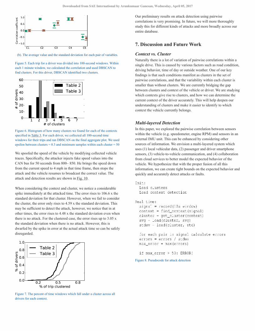
(b). The average value and the standard deviation for each pair of variables.

Figure 5. Each trip for a driver was divided into 100-second windows. Within each 1 minute window, we calculated the correlation and used DBSCAN to find clusters. For this driver, DBSCAN identified two clusters.

Figure 6. Histogram of how many clusters we found for each of the contexts specified in Table 3. For each driver, we collected all 100-second time windows for their trips and ran DBSCAN on the final aggregate plot. We used epsilon between clusters = 0.3 and minimum samples within each cluster = 50

We spoofed the speed of the vehicle by modifying collected vehicle traces. Specifically, the attacker injects fake speed values into the CAN bus for 50 seconds from 800– 850. He brings the speed down from the current speed to 4 mph in that time frame, then stops the attack and the vehicle resumes to broadcast the correct value. The attack and detection results are shown in Fig. 10.

When considering the context and cluster, we notice a considerable spike immediately at the attacked time. The error rises to 106.6 x the standard deviation for that cluster. However, when we fail to consider the cluster, the error only rises to 4.59 x the standard deviation. This may be sufficient to detect the attack, however, we notice that in at other times, the error rises to 4.48 x the standard deviation even when there is no attack. For the clustered case, the error rises up to 3.05 x the standard deviation when there is no attack. However, this is dwarfed by the spike in error at the actual attack time so can be safely disregarded.

Figure 7. The percent of time windows which fall under a cluster across all drivers for each context.

Our preliminary results on attack detection using pairwise correlations is very promising. In future, we will more thoroughly study this for different kinds of attacks and more broadly across our entire database.

7. Discussion and Future Work

Context vs. ClusterNaturally there is a lot of variation of pairwise correlations within a single drive. This is caused by various factors such as road condition, driving behavior, time of day or outside weather. One of our key findings is that such conditions manifest as clusters in the set of pairwise correlations, and that the variability within each cluster is smaller than without clusters. We are currently bridging the gap between clusters and context of the vehicle or driver. We are studying which contexts give rise to clusters, and how we can determine the current context of the driver accurately. This will help deepen our understanding of clusters and make it easier to identify to which context the vehicle currently belongs.

Multi-layered DetectionIn this paper, we explored the pairwise correlation between sensors within the vehicle (e.g. speedometer, engine RPM) and sensors in an external IMU unit. This can be enhanced by considering other sources of information. We envision a multi-layered system which uses (1) local vehicular data, (2) passenger and driver smartphone sensors, (3) vehicle-to-vehicle communication, and (4) collaboration from cloud services to better model the expected behavior of the vehicle. We hypothesize that with the proper fusion of all this information, we can create tight bounds on the expected behavior and quickly and accurately detect attacks or faults.

Figure 8. Pseudocode for attack detection


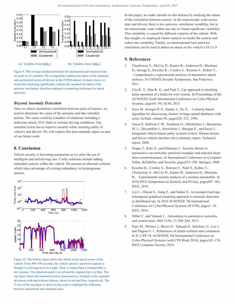
(a). Variables from Table 3 (b). Variables from Table 2

Figure 9. The average standard deviation for unclustered and clustered trips for each set of variables. We averaged the standard deviation of the clustered and unclustered across all drivers in the IVBSS dataset. In many cases, we found that clustering significantly reduces the standard deviation of the pairwise correlation, therefore making it a promising technique for attack detection.

Beyond Anomaly DetectionOnce we detect anomalous correlation between pairs of sensors, we need to determine the cause of the anomaly and take remedial actions. The cause could be a number of situations including a malicious attack, ECU fault or extreme driving conditions. Any remedial action has to improve security while ensuring safety of vehicles and drivers. We will explore this post-anomaly aspect as part of our future work.

8. ConclusionVehicle security is becoming paramount as we enter the era of intelligent and self-driving cars. Costly solutions include adding redundant sensors within the vehicle. We present an alternate solution which takes advantage of existing redundancy in heterogenous sensors.

Figure 10. The bottom figure shows the attack on the speed sensor of the vehicle. From 800–850 seconds, the vehicle speed is spoofed to appear as though it is slowing down to 4 mph. Then, it returns back to normal after a few minutes. The attacked signal is in red and the original trip is in blue. The top figure shows the normalized error (measured as a multiple of the standard deviation) with and without clusters, shown in red and blue, respectively. The Y axis of the top figure is drawn in log scale to highlight the difference between unclustered and clustered cases.

In this paper, we make inroads on this defense by studying the nature of the correlation between sensors. In the macroscopic scale across trips and drivers, there is low pairwise correlation variability, but in the microscopic scale within one trip we found significant variability. This variability is caused by different contexts of the vehicle. With this insight, we employed cluster analysis to model the context and reduce the variability. Finally, we demonstrated how pairwise correlation can be used to detect an attack on the vehicle’s ECUs.9.

9. References1. Checkoway S., McCoy D., Kantor B., Anderson D., Shacham

H., Savage S., Koscher K., Czeskis A., Roesner F., Kohno T., . Comprehensive experimental analyses of automotive attack surfaces. In USENIX Security Symposium. San Francisco, 2011.

2. Cho K.-T., Shin K. G., and Park T.. Cps approach to checking norm operation of a brake-by-wire system. In Proceedings of the ACM/IEEE Sixth International Conference on Cyber-Physical Systems, pages41–50. ACM, 2015.

3. Ester M., Kriegel H.-P., Sander J., Xu X., . A density-based algorithm for discovering clusters in large spatial databases with noise. In Kdd, volume 96, pages226–231, 1996.

4. Green P., Sullivan J. M., Tsimhoni O., Oberholtzer J., Buonarosa M. L., Devonshire J., Schweitzer J., Baragar E., and Sayer J.. Integrated vehicle-based safety systems (ivbss): Human factors and driver-vehicle interface (dvi) summary report. Technical report, 2008.

5. Hoppe T., Kiltz S., and Dittmann J.. Security threats to automotive can networks–practical examples and selected short-term countermeasures. In International Conference on Computer Safety, Reliability, and Security, pages235–248. Springer, 2008.

6. Koscher K., Czeskis A., Roesner F., Patel S., Kohno T., Checkoway S., McCoy D., Kantor B., Anderson D., Shacham H., . Experimental security analysis of a modern automobile. In 2010 IEEE Symposium on Security and Privacy, pages447–462. IEEE, 2010.

7. Liu C., Ghosal S., Jiang Z., and Sarkar S.. An unsupervised spatiotemporal graphical modeling approach to anomaly detection in distributed cps. In 2016 ACM/IEEE 7th International Conference on Cyber-Physical Systems (ICCPS), pages1–10. IEEE, 2016.

8. Miller C. and Valasek C.. Adventures in automotive networks and control units. DEF CON, 21:260–264, 2013.

9. Pajic M., Weimer J., Bezzo N., Tabuada P., Sokolsky O., Lee I., and Pappas G. J.. Robustness of attack-resilient state estimators. In IC-CPS’14: ACM/IEEE 5th International Conference on Cyber-Physical Systems (with CPS Week 2014), pages163–174. IEEE Computer Society, 2014.


AcknowledgementsThe work reported in this paper was supported in part by the National Science Foundation under Grants CNS-1505785 and CNS-1646130, and by a Ford-UM Alliance Program.

The Engineering Meetings Board has approved this paper for publication. It has successfully completed SAE’s peer review process under the supervision of the session organizer. The process requires a minimum of three (3) reviews by industry experts.

All rights reserved. No part of this publication may be reproduced, stored in a retrieval system, or transmitted, in any form or by any means, electronic, mechanical, photocopying, recording, or otherwise, without the prior written permission of SAE International.

Positions and opinions advanced in this paper are those of the author(s) and not necessarily those of SAE International. The author is solely responsible for the content of the paper.

ISSN 0148-7191

http://papers.sae.org/2017-01-1654


http://papers.sae.org/2017-01-1654

exploiting consistency among heterogeneous …...exploits the natural redundancy amongst...

Documents