exploring a neurological model for cross-cultural consonance and dissonance in music perception: cse...

7/28/2019 Exploring a Neurological Model for Cross-Cultural Consonance and Dissonance in Music Perception: CSE 258A Proj…

http://slidepdf.com/reader/full/exploring-a-neurological-model-for-cross-cultural-consonance-and-dissonance 1/12

1

Exploring a Neurological Model for Cross-Cultural Consonance and Dissonance in

Music Perception:

CSE 258A Project Final Report

Clifford Champion ([email protected])

Department of Computer Science, UCSDSan Diego, CA, USA

Eric Morgan ([email protected])Department of Computer Science, UCSD

San Diego, CA, USA

Abstract

In this project we will explore a neurological explanation for the cross-cultural tendencies to form tuning systems andqualitatively “consonant” musical harmonies according tosimilar, seemingly innate, rules. Efforts will be largely basedon recent research which uses multi-layer neural networks of non-linear oscillators. We will recreate a selection of resultsfrom two recent papers, and in the course of doing consider indetail to what extent the results support a theory of cross-cultural tonality. Based on our results, we are convinced thereare likely inherent biases in our auditory system towardcertain specific harmonies, supporting a cross-culturalhypothesis.

Keywords: tonality; cognition; dissonance; music

Background

Tonal theory is the study of how pairs of tones, either

played simultaneously or consecutively, tend to be

perceived qualitatively as consonant or dissonant.

Consonance is generally described as stable, calming, or pleasant; while dissonance as unstable, attractive (of a

different tone to follow), unsettling, or unpleasant. Different

pairs of tones (at different musical intervals) are not

necessarily described consistently across cultures.

Tonal theory has gone through a number of radical

changes over time (Large, 2011). Pythagoras proposed a

small integer ratio (SIR) theory, that tone pairs (a harmony)

whose frequencies are not related by an SIR sound

dissonant, while those that are sound consonant. However,

as of the 19th century most instrument tunings use small

irrational ratios for each needed frequency, not integer ratios

(see Appendix B). The SIR theory could be modified to

include SIR-approximates, but there are many of these, andat what threshold to begin excluding not “small” enough

ratios is unclear. In any case, SIR theory does not offer

explanation for why SIRs (or irrational approximates) don’t

appear equally often cross-culturally, for instance there are

SIR-tuned notes present in the basic musical scales and

tuning systems of gamelan music from Indonesia, and in

traditional Chinese music, which are not present in the

western 12-tone scale and vice-versa.

Helmholtz, a 19th century physicist and physician

proposed that the auditory system essentially performed a

Fourier transform (Large, 2011). In the frequency-domain,

small integer ratios have no special or unique meaning, a

relativistic understanding that is incompatible with SIR

theory. Helmholtz then theorized that “sensory dissonance”

occurred when waveforms of pure tones interfered at critical

frequencies. However, one problem with Helmholtz’ theoryis that dissonant frequency pairs can only manifest for

simultaneous tones, not consecutive tones, yet consonance

and dissonance tend to be attributed (by listeners) to tone

sequences as well, not just simultaneous tones.

Modern Tonal Theory continues with the assumption

that SIRs have minimal or no special importance. Modern

Tonal Theory builds upon Helmholtz’ theory by assuming

that consonance and dissonance are largely cultural, and that

a mapping is learned which transforms tone pair intervals

(frequency ratios) into symbols at higher-levels of the

auditory system, according to the musical characteristics

which people hear most often (i.e. the music of their own

culture).

Figure 1: The neurological pathways of the human auditory

processing (Patel & Iversen, 2007).



2013 June 8

2

However, Modern Tonal Theory cannot explain why

cross-culturally, SIR (or approximate-SIR) intervals are

disproportionately more common (compared to random) in

instrument tunings and thus the music of each culture

(Burns, 1999). Thus there may be ounces of truth to both

Modern Tonal Theory and SIR theory.

Relatively recent discoveries of the auditory system

show that at multiple levels our audio processing is very

likely non-linear (Eguiluz, Ospeck, Choe, Hudspeth, &

Magnasco, 2000; Langner, 1992; Joris, Schreiner, & Rees,

2004; Lee, Skoe, Kraus, & Ashley, 2009). Non-linear

oscillatory responses can exhibit interesting properties such

as entraining to frequencies in the stimulus nearby to their

natural frequency (which may account for perceived

interchangeability of SIRs with approximate SIRs), and a

variety of other response frequencies, such as a sub-

harmonic frequencies (e.g. 1/2 of the neural oscillator’s

natural frequency). Non-linear behavior is known to be

possible using a pairs of inhibitory neurons (Taylor,

Cottrell, & Kristan, 2002) or of inhibitory and excitatoryneurons, such that their combined output spike rate exhibits

oscillation, essentially a form of frequency modulation

(similar to FM radio for instance). To model this neural

oscillator pair, a single complex variable is often

used, where represents both the current phase of the

frequency modulation (via or its angle on the

complex plane), as well as the peak frequency or peak spike

rate (via its magnitude).

Figure 2: Example of a 4-Layer GFNN (Large, 2011). Each

layer is composed of neural oscillators tuned across multiple

octaves of frequencies.

In various papers (Large, 2011; 2012), Large contends

three things: 1) explain the cross-cultural SIR-bias in tuning,

2) simulate learned differences in the presence or absence of

theoretical SIRs in cultural differences, and 3) predict tonal

attraction and thus predict “consonance”.

In a simple but interesting construction by Large, two

layers of neural oscillators were used: the first representing

the cochlear cells of the inner ear, and the second the dorsal

cochlear nucleus (DCN). Each layer forms what Large calls

a gradient-frequency neural network, and is simply an array

of neural oscillators, each “tuned” to a different frequency

forming a gradient of oscillators across a spectrum of

frequencies. Such a two-layer network can produce output

which not only responds to matching input frequencies, but

also with approximate and SIR frequencies. This suggests

the non-linearity of the model inherently exhibits special

sets of SIR tone pairs which are complementary, a natural

(unlearned) behavior of the simulation which runs contrary

to Helmholtz’ theory or Modern Tonal Theory.

In these multi-layer GFNNs, which in some of Large’s

experiments involve up to 4-layers to include A1, the

middle or upper layers are configured differently (than the

cochlea layer) so as to exhibit dynamically appearing limit

cycles. These limit cycles manifest after sufficient stimuli,

and act as a tonal memory, where the limit cycle frequencies

(the most active neural oscillators’ frequencies) persist in

the absence of further stimuli. Which frequencies appear as

limit cycles also appears to be a function of learnedconnection weights, and Large hypothesizes this may

explain the cultural differences in instrument tunings.

Large has conducted earlier experiments with Hebbian

learning between and within each GFNN layer, showing

stronger associations forming between harmonies “heard”

more often. In order to perform Hebbian learning between

oscillating nodes, Large expands on Hebbian learning for

neural oscillators originally derived by Hoppensteadt &

Izhikevich (1996).

Hoppensteadt & Izhikevich showed that for a pair of

neural oscillators, one feeding forward to the other, that a

complex-valued connection weight

can not only

enforce a phase differences between two oscillators but canalso learn this phase difference over time using a

generalization of Hebbian learning. Hoppensteadt showed

that for a collection of neural oscillators, each with output [ ], each feeding into a neural oscillator and all with identical frequencies , e.g.

( ) ∑

that synaptic weights can be modified using the update

rule

where is the fade rate and is a function of

plasticity rate and other fixed properties of the neural

oscillators. is a parameter of the oscillator which turns

non-linear behaviors on or off, and are discussed in more

detail later. determines the oscillation rate and is

proportional to the natural frequency of the neural oscillator

(in Hz). The notation refers to the complex conjugate of .

Note that the multiplication of with produces a

complex value whose magnitude is the product of their



2013 June 8

3

magnitudes, but whose angle on the complex plane is equal

to their phase difference. As is learned, (), or the

angle which makes on the complex plane, acts to impose

or reinforce a phase difference between neural oscillators and , while determines the strength of the oscillatory

coupling connection between

and

. In this simple case,

oscillators which oscillate together often, will increase their connection weight such that they will be more likely to

oscillate together in the future.

For Large’s model, which attempts to learn weights

between neural oscillators of not just identical center

frequencies but also different , Hoppensteadt’s weight

update rule is insufficient. Large derives an expanded

update rule (Large, 2010) which alters the connection

similarly as above, but also does so whenever higher-order

resonances are active between the neural oscillators as well,

√ √

where [] is an additional parameter specifying the

degree of non-linearity used for learning. The effect of

learning connections weights in this case is more interesting.

Recall that the non-linear behavior of neural oscillators

causes them to respond to frequencies related to their natural

frequency by an SIR. For each pair of connected neural

oscillators (for instance from a cochlea layer to a DCN

layer), some will naturally oscillate strongly together (e.g.

those with a 1:1 or 2:1 relationship), some will only

moderately (e.g. all other SIR relationships, in varying

degrees), and others (non-SIR) not at all. In particular, the

modified Hebbian rule (Eq. 3) will increase the effects of

future interactions between SIR-related oscillator pairs, for the SIR frequencies heard most often during training. For

example, the unlearned output behavior of hearing a western

Perfect 4th harmony (4:3 frequency ratio) will be small but

significant in an untrained system; but over repeated

exposure, the response by oscillators specific to this SIR

harmony (4:3) should become much stronger than for SIRs

not seen during training.

Project Motivation

Three publications by Large et al. (Large, 2010; Large,

2011; Large & Almonte, 2012) show promise in explaining

both the cross-cultural bias toward SIR tone pairs (and

learned or cultural differences), and tonal consonance due tonon-linear SIR resonances and memory. Large has

conducted experiments across a modest set of tone pairs and

changing harmonies, essentially three of particular note: a

constant minor 3rd using synthesized just intonation (a

precise SIR tuning method common pre-18th century), a

constant minor 3rd using samples from an electric piano

with equal temperament tuning (an approximate SIR tuning

method common post-18th century, where all notes are

separated by a constant multiple), and a C Major triad

followed by a B (7 th “leading”) tone. Both tuning methods

are expected to show similar results. Though equal

temperament tuning does not involve SIRs, their

approximate values are expected to be near enough to their

true SIR such that the nonlinear entrainment will respond as

if truly a SIR. Appendix B has more detail on each tuning

method.

The motivation behind the project proposal presented

herein is ultimately to broaden Large’s experiment set to

include experiments involving all 12 chromatic intervals

(from a common tonic) e.g. minor 3rd, Major 3rd, Perfect 4th,

etc., as simultaneous tone pairs, recreating his given results

in the process. The output layer behavior for each tone pair,

as well as the results of Hebbian learning, will be compared

with available, qualitative descriptions for each 12 tone

pairs (available in Large’s papers and in others). Building

upon Large’s findings, we want to observe whether

“consonant” tone pairs tend to have fewer activated outputs,

while qualitatively dissonant tone pairs tend to have more

activated outputs; or whether any other pattern or

correlation manifests.

Project Phases

Tone Synthesis and Multi-Layer NN Construction

Tasks to be completed: (1) implementation or integration

with a module for tone synthesis (to create test tones), with

harmonics, at arbitrary frequencies; (2) implementation of a

multi-layer, non-linear oscillating neural network according

to the differential equations provided (Large, 2011; Large et

al., 2010) and using a forward numerical integrator to

compute the dynamical system over time; (3) setup of

development environment and debugging tools.

Learning/Configuration and Re-creation of Large

Results

Tasks to be completed: (1) the model configuration and

setup necessary to recreate the Large results; (2) the re-

creation of the Large results using the minor 3rd

simultaneous tones.

Expanded Experiments

Tasks to be completed: (1) tests of the model using all 12

chromatic intervals played as simultaneous tones; (2) tests

of the model using all 12 intervals but as consecutive tones

instead of simultaneous tones; (3) the comparison of outputlayer activations with qualitative descriptions of tone pairs.

Preparation of Findings

Tasks to be completed: (1) preparation of findings, creation

of charts, final report editing.



2013 June 8

4

Preliminary Work

Development Environment and Process

Development environments are configured for all team

members, utilizing Visual Studio 2012 for code authoring

and debugging, SVN for source code management, and

Google Spreadsheets for project tracking and tasking.

Object-Oriented Model for Dynamical Systems

A custom data model in C#/.NET is created for representing

dynamical systems, complex-valued nodes, numerical

integrators, and various other primitives and helper classes;

our key base types are DynamicalSystem, DynamicalNode,

IIntegrator , and VectorOI . Our base types are discussed in

more detail in Appendix C. Each differential equation

needed for our simulations is implemented as part of

overriding function F(t, y) in subclasses of DynamicalNode,

corresponding to 1st-order differential equations of the form

[ ]

.

Numerical Integration

For numerical integration we have written a custom

implementation of fourth-order Runge-Kutta, named

RungeKuttaIntegrator (RKI) and implementing our

IIntegrator interface. Though RK packages for .NET exist,

they are not necessarily trivial to integrate with our sparse,

object-oriented model for the dynamical system; RK is a

fairly simple algorithm to implement, thus a judgment call

was made to quickly prepare our own implementation.To initially test our RKI, we have a simple subclass of

DynamicalSystem called LinearCoupleSystem, composed

instances of LinearNode, a concrete subclass of

DynamicalNode. This is a two-node system, coupled and

configured to exhibit a stable, intrinsic oscillation.

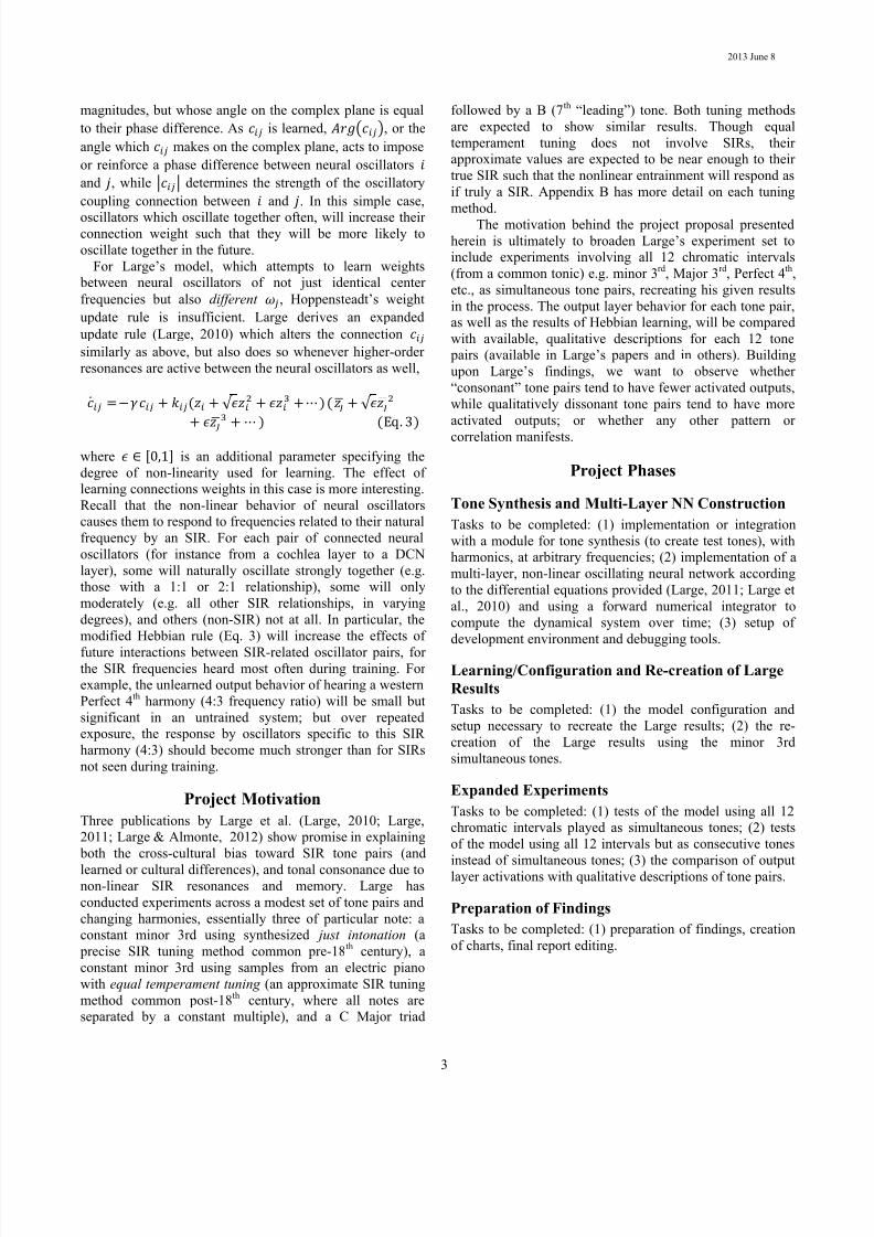
For this simple two node system, RKI computes 90,000

iterations per second. Step sizes between 0.01 and 0.00001all show stable oscillation as expected for this system.

Figure 3 shows our example output used to preliminarily

validate the correctness of RKI.

User Interface

Our user interface is constructed to be functional for our

simulation and debugging needs. Visually it consists of two-

panes (see Figure 15), one devoted to a textual, time-

sequential log of system state, sampled regularly; and the

other pane devoted to a (tabbed) choice of visual

representations of the current system, including node

magnitudes, node magnitudes over time, and connection

weights. Our application runs over multiple threads, with

details discussed in Appendix C.

Figure 3: Node output of LinearPairSystem. Variables #, τ,

u, and v are iteration count, model time, linear node 1, and

linear node 2 respectively.

Audio Synthesis and Rendering

In order to simulate an external sound stimulus, we haveagain subclassed DynamicalNode, creating a class we call

ToneNode. ToneNode is designed to encapsulate a single

audio source in the world, which may be emitting any

number of notes of different pitches, and each note

composed of a different set of harmonics. As you might

expect, ToneNode.F(t, y) computes the numerical derivative

of a superposition of zero or more sine waves at various

frequencies and amplitudes.

In order to verify that our ToneNode generates correct

wave displacement values over time, and in order to aid in

validation and debugging for the project overall, we utilized

a 3rd party library for .NET which enables easy output of

PCM sound data to the computer’s soundcard and speakers.In order to render this sound, as ultimately computed by our

Runge-Kutta integrator, we did two things. We expanded

our numerical integration background thread to also append

the latest Value of ToneNode, as computed after each

integration step, to our audio output module. We choose a

step size that matches standard sound card sample rates

(44.1 KHz), and create a single-node system

ToneTestSystem. Because the single node system can be

integrated faster than the rate at which the audio will play

back at real-time (for the chosen 44.1 KHz sample rate), we



2013 June 8

5

are able to advance the system and hear the system in real-

time without gaps or much lead-time. We subjectively tested

different configurations of notes (different fundamental

frequencies and harmonics lists), including a pure 440 Hz

tone, often used in musical tuning. In particular, the 440 Hz

tone sounded identical to that of the sample 440 Hz tone as

available on Wikipedia. This validates that our ToneNode

generates correct output, and further (though marginally so)

validates the correctness of our RKI implementation.

Simulating the Auditory System

Recreating Large, Almonte, Velasco 2010

As a first major step toward recreating the results of Large’s

multi-layer neural network, we first recreated the results of

his earlier 1-layer network (Large, Almonte, & Velasco,

2010). This 1-layer network is fed from a single input node,

oscillating a real-valued stimulus at a pure sine 1 Hz and 0.3

amplitude, to a collection of 360 neural oscillators

representing a simple model of the cochlea. The

configuration replicated is a collection of nodes spanning 6

octaves (from 0.125 Hz to 8 Hz), with 60 nodes per octave,

each node spaced linearly over the log of the frequency

space. Large calls this in general a “gradient-frequency

neural network” or GFNN.

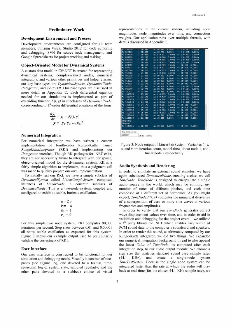
Figure 4: Original results of Large et al. 2010. The y-axis is

the log-frequency space of neural oscillators, the x-axis is

time, and black indicates strong response (average

magnitude).

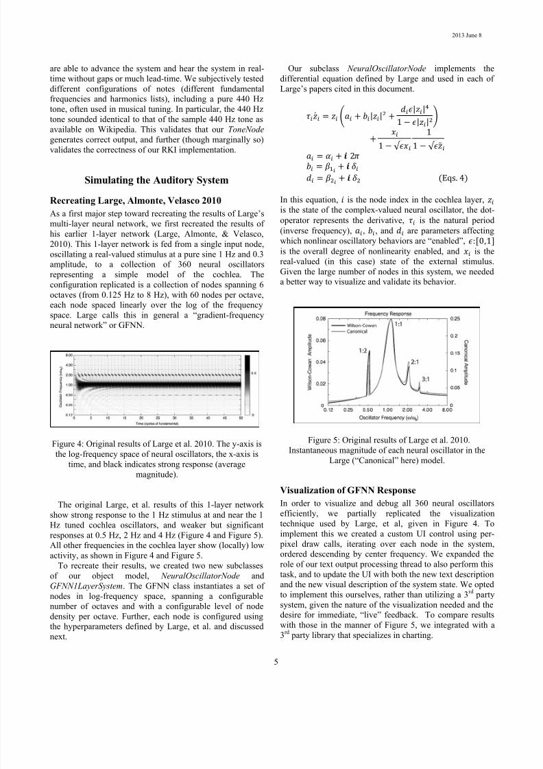
The original Large, et al. results of this 1-layer network

show strong response to the 1 Hz stimulus at and near the 1

Hz tuned cochlea oscillators, and weaker but significant

responses at 0.5 Hz, 2 Hz and 4 Hz (Figure 4 and Figure 5).All other frequencies in the cochlea layer show (locally) low

activity, as shown in Figure 4 and Figure 5.

To recreate their results, we created two new subclasses

of our object model, NeuralOscillatorNode and

GFNN1LayerSystem. The GFNN class instantiates a set of

nodes in log-frequency space, spanning a configurable

number of octaves and with a configurable level of node

density per octave. Further, each node is configured using

the hyperparameters defined by Large, et al. and discussed

next.

Our subclass NeuralOscillatorNode implements the

differential equation defined by Large and used in each of

Large’s papers cited in this document.

|| || ||

√ √

In this equation, is the node index in the cochlea layer, is the state of the complex-valued neural oscillator, the dot-

operator represents the derivative, is the natural period

(inverse frequency), , , and are parameters affecting

which nonlinear oscillatory behaviors are “enabled”, [] is the overall degree of nonlinearity enabled, and is the

real-valued (in this case) state of the external stimulus.

Given the large number of nodes in this system, we neededa better way to visualize and validate its behavior.

Figure 5: Original results of Large et al. 2010.

Instantaneous magnitude of each neural oscillator in the

Large (“Canonical” here) model.

Visualization of GFNN Response

In order to visualize and debug all 360 neural oscillators

efficiently, we partially replicated the visualization

technique used by Large, et al, given in Figure 4. To

implement this we created a custom UI control using per-

pixel draw calls, iterating over each node in the system,

ordered descending by center frequency. We expanded the

role of our text output processing thread to also perform this

task, and to update the UI with both the new text description

and the new visual description of the system state. We opted

to implement this ourselves, rather than utilizing a 3 rd party

system, given the nature of the visualization needed and the

desire for immediate, “live” feedback. To compare results

with those in the manner of Figure 5, we integrated with a

3rd party library that specializes in charting.



2013 June 8

6

Validation of Neural Oscillator Implementation

Armed with a better way of visualizing the system behavior,

we compared our system with that of Large, et al. We tested

with both a 360-node configuration, and a 720-node

configuration for higher fidelity. Both systems generated

nearly identical results, and we present images of the 720-

node configuration for more clarity. In their paper they donot discuss their numerical integration method, nor step

size. We experimented with different step sizes for our RKI,

and for now settled on 0.001 seconds, which at any further

granularity seems to offer no further major changes in

behavior. At 720 nodes in the system, our RKI can calculate

approximately 260 iterations per second. After a couple

rounds of debugging our implementation of the differential

equation, our expected results turned up and are captured in

Figure 6 and Figure 7.

Figure 6: Our re-creation of Figure 4 using

GFNN1LayerSystem. Stimulus frequency and amplitude are1 Hz and 0.3. Our results share characteristics of sub-

harmonic and harmonic response.

Our hyperparameters used (with respect to Eqs. 4) are

chosen to be identical to that of Large et al. 2010. These are

This configuration should permit the neural oscillators to

respond to SIR stimulus for stimulus amplitudes only above

a certain levels, as predicted by the Andronov-Hopf

bifurcation analysis (Large 2010).

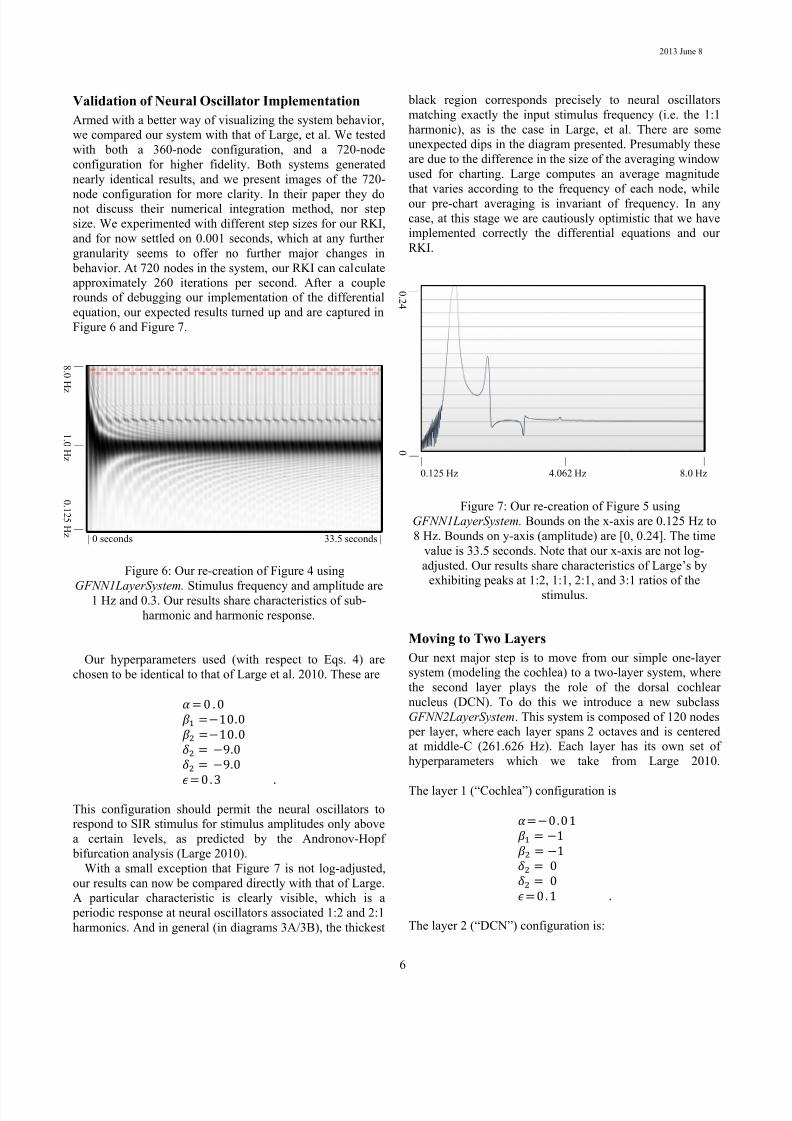
With a small exception that Figure 7 is not log-adjusted,

our results can now be compared directly with that of Large.

A particular characteristic is clearly visible, which is a

periodic response at neural oscillators associated 1:2 and 2:1

harmonics. And in general (in diagrams 3A/3B), the thickest

black region corresponds precisely to neural oscillators

matching exactly the input stimulus frequency (i.e. the 1:1

harmonic), as is the case in Large, et al. There are some

unexpected dips in the diagram presented. Presumably these

are due to the difference in the size of the averaging window

used for charting. Large computes an average magnitude

that varies according to the frequency of each node, while

our pre-chart averaging is invariant of frequency. In any

case, at this stage we are cautiously optimistic that we have

implemented correctly the differential equations and our

RKI.

Figure 7: Our re-creation of Figure 5 using

GFNN1LayerSystem. Bounds on the x-axis are 0.125 Hz to

8 Hz. Bounds on y-axis (amplitude) are [0, 0.24]. The time

value is 33.5 seconds. Note that our x-axis are not log-

adjusted. Our results share characteristics of Large’s by

exhibiting peaks at 1:2, 1:1, 2:1, and 3:1 ratios of the

stimulus.

Moving to Two Layers

Our next major step is to move from our simple one-layer

system (modeling the cochlea) to a two-layer system, where

the second layer plays the role of the dorsal cochlear

nucleus (DCN). To do this we introduce a new subclass

GFNN2LayerSystem. This system is composed of 120 nodes

per layer, where each layer spans 2 octaves and is centered

at middle-C (261.626 Hz). Each layer has its own set of

hyperparameters which we take from Large 2010.

The layer 1 (“Cochlea”) configuration is

The layer 2 (“DCN”) configuration is:

| 0 seconds 33.5 seconds |

|

|

|

8.0H

z

1.0Hz

0.125Hz

|

|

0.24

0

| | |

0.125 Hz 4.062 Hz 8.0 Hz



2013 June 8

7

Whether each hyperparameter is less than 0, equal to 0, or

greater than 0 is important in turning on and off different

non-linear behaviors. Layer 1 is configured qualitatively

similar to as it was in our GFNN1LayerSystem. Layer 2 here

however is configured in such a way as to exhibit memory,

by continuing to oscillate at frequencies which were

sufficiently present in the stimulus, even in the subsequent

absence of that stimulus (i.e. in later silence). After

upgrading our user-interface to support easily altering the

stimulus while a simulation is ongoing, we quickly

constructed a test to see if a form of tonal memory was

present. For this quick test we connected nodes in layer 1 to

nodes in layer 2 in a 1:1 fashion according to matching

frequency, with a constant connection weight. We then

stimulated this system with a Major triad at middle-C (i.e. a

C-E-G harmony), then disabled the stimulus halfway into

the simulation.

Figure 8: Output of layer 2. A “C-E-G major triad”

stimulus (starting at Middle C or 261.626 Hz) was enabled

for the first half of the pictured time period.

As visible in Figure 8, after the stimulus is disabled, the

neural oscillators at layer 2 (contrary to layer 1, not pictured

here) continue to activate for some time before fading. This

indicates the hyperparameters are enabling a form of tonal

memory at layer 2.

Hebbian Learning

The final step in recreating the desired two-layer results is to

introduce connection weight learning. In Large 2011,

Hebbian learning is performed on internal connections in

layer 2 only. To expand our system to support Hebbian

learning, we introduce a ConnectionWeightSystem subclass

of DynamicalSystem. This system is paired with

GFNN2LayerSystem, such that the combined dynamical

system is solved by solving each system in alternation, i.e.

first we solve for the neural oscillator values at time

using

constant connection weights from time , and then we

solve for connection weights at time using constant

oscillator values from time , and so on. Our connection

weight system is itself composed of instances of subclasses

of DynamicalNode, specialized to implement Eq. 3 for

updating connection weights . In total this system has

480 dynamic nodes, and 56,600 dynamic connection

weights).

Figure 9: Original results (Large 2011) of complex-valuedHebbian learning on the internal connection weights for

layer 2 after hearing a constant minor 3 rd harmony as

stimulus.

The stimulus for Large’s first Hebbian learning

experiment is a minor 3rd harmony (500 and 600 Hz), each

with 5 harmonics including the fundamentals, for a total set

of stimulus frequencies amounting to 500 Hz, 1 kHz, 1.5

kHz, 2 kHz, 2.5 kHz, 600 Hz, 1.2 kHz, 1.8 kHz, 2.4 kHz,

and 3.0 kHz, which we utilize for this experiment as well.

The inclusion of 5 harmonics per note (4 overtones per note)

is a more realistic real-world stimulus, similar to what mightcorrespond to a wind or chime instrument. The result of

Hebbian learning on the internal connections of layer 2 in

our simulation should hopefully produce results similar to

those depicted in Figure 9.

After configuring for the new stimulus characteristics, our

results are depicted in Figure 10. We were not able to

determine the values originally used for Hebbian decay and

plasticity ( and in Eq. 3), nor what relative amplitudes

were used for each of the 10 harmonics in the stimulus.

Thus at this point we attribute the discrepancies between

| 0 seconds 0.15 seconds |

|

|

|

523.2Hz

26

1.6Hz

130.8Hz



2013 June 8

8

Figures 9 and 10 to differences in the above parameters, that

may actually differ by an order of magnitude or more. For

this experiment we used , an amplitude of 0.5 for

the fundamental frequencies, and an inverse fall-off for the

amplitudes of the overtone frequencies (e.g. 0.5 amplitude

for 500 Hz and 600 Hz; 0.25 amplitude for 1 kHz and 1.2

kHz, etc.) which is not an uncommon amplitude fall-off

model for naturally occurring overtones. Something else we

are not analytically equipped with provided with in the

model description is a stopping condition or convergence

conditions for learning, thus at present our Hebbian learning

eventually increases weights to such a point that the entire

system diverges to infinity.

In spite of all of this, Figure 10 does show the neural

oscillator version of Hebbian learning in fact strengthening

the connections between pairs of neural oscillators

corresponding to pairs of harmonics in the minor 3rd

stimulus.

Figure 10: Our results of a partial re-creation of Figure 9.

The top-right and bottom-left dark regions correspond to

weights learned by and reinforcing the minor 3 rd harmony.

Testing for a Small-Integer Ratio Bias

Pressing on, we lastly set out to compare different stimuli,

looking for the presence or absence of a bias toward SIR-

based harmonies.

According to an analysis of higher-order resonances

between oscillator pairs (Large, 2011), pairs with “simple”

frequency ratios such as 1:1 or 3:2 should co-activate more

strongly than pairs with other ratios such as 9:5 or 16:15.

The full analysis can form an ordering over the (countably

infinite) set of ratios, according to their higher-order

compatibility, which turns out also to be a good predictor of

human descriptions of “consonance” (e.g. 1:1, 1:2) and

“dissonance” (e.g. 16:15 and 15:8).

In a novel experiment of our own, we decided to re-run

the 2-layer, Hebbian-enabled, experiment but with two new

stimuli, tested and trained on separately as part of two runs.

The motivation for this experiment is to test whether there

are significant differences in the results of Hebbian learning,

according to whether the stimulus harmony is consonant or

dissonant . To find no perceivable or correlatable differences

would be a result compatible with Modern Tonality Theory,

that learning any harmony is no different than learning any

other harmony; while to find the contrary may support an

inherent bias toward SIR harmonies.

For the construction of this experiment, our first stimulus

is formed from a Perfect 5 th harmony with the first

fundamental frequency at 500 Hz (same as the previous

Hebbian experiment), and second fundamental frequency at

750 Hz (according to the 3:2 JI tuning ratio for a Perfect 5 th,

e.g. notes C-G). Our second stimulus, enabled and trained

on separately, is formed from a diminished 5 th harmony withthe first fundamental frequency again at 500 Hz, while the

second fundamental frequency is at 707.11 Hz (according to

the approximate 45:32 ET tuning ratio for a diminished 5 th,

e.g. notes C-F#). Both stimuli include 4 overtones with an

inverse amplitude drop-off, as was used in the previous

experiment.

We keep the same “tonic” (500 Hz) as in the previous

experiment for consistency and comparability. We choose to

compare the Perfect 5th and diminished 5th as our new

stimuli because of their particular characteristics in the

western 12-stone scale and to western listeners: (1) they are

chromatic neighbors, e.g. F# is immediately followed by G,

and thus their absolute frequencies (in Hz) are relativelyclose to one another; and (2) they are qualitatively quite

opposite in terms of consonance, e.g. C-G is generally

described as one of the most consonant harmonies on the

12-tone scale, while C-F# is generally described as one of

the most dissonant.

Figures 11 and 12 show the state of layer 2 after some

time with the Perfect 5 th and diminished 5th stimuli

respectively. Figures 13 and 14 show the results of Hebbian

learning in layer 2, as was shown in the previous Hebbian

experiment. Qualitatively, the learning results appear very

similar. However, the connection weight magnitudes differ.

In the Perfect 5th results (Figure 13), the black clusters of

strong connections have magnitudes tightly bounded by0.025023, while in the diminished 5 th results (Figure 14) the

same corresponding strong connection clusters have

magnitudes tightly bounded by 0.021871, or 87.4% of that

in the former. From this experiment alone, it is difficult to

say precisely what the difference is attributable to (as it may

also be related to different frequencies responding

differently numerically and the accumulation of numerical

error).

| | |250 Hz 1 kHz 4 kHz

|

|

|

250Hz

1kHz

4kHz



2013 June 8

9

Figure 11: Two-layer GFNN with Perfect 5 th stimulus (2

notes, each with 5 harmonics), 500 Hz and 750 Hz tonics.

Figure 12: Two-layer GFNN with diminished 5 th stimulus

(2 notes, each with 5 harmonics), 500 Hz and 707.11 Hz

tonics.

|

|

|

4kHz

1kHz

250Hz

|

|

|

4kHz

1kHz

250H

z



2013 June 8

10

However, there are some important visible differences in

Figures 11 and 12 which support that the difference in the

harmony ratios (3:2 vs. 45:32) is in fact the cause of the

difference in learning. Especially for the higher-frequencies

in the layer 2 response, there are more overlaps in the

Perfect 5th results than there are in the diminished 5 th. This is

visible by the relative calmness at the high-frequency region

in Figure 11 as opposed to the complexity in that same

region in Figure 12. This is expected mathematically, as the

first higher-order response to the 3:2 note is in fact the same

frequency as the second higher-response to the 1:1 note,

effectively 3:1. Further, each of the four overtones of each

note in the Perfect 5th coincides similarly. In contrast, the

relationship between the 45:32 note and its tonic in the

diminished 5th offer virtually no coinciding frequencies.

Thus where the amplitudes of each harmonic in the Perfect

5th stimulus would have an additive effect, such an effect is

absent in the diminished 5th stimulus. Our Hebbian update

rule (Eqs. 3) is positively affected by oscillator amplitude,

thus there is an analytical explanation for why the

diminished 5th did not form quite as strong of connectionweights for the 45:32 stimulus ratio. This is consistent with

the hypothesis that small integer ratios have inherent special

properties in this auditory simulation and GFNNs.

Figure 13: Learning results with Perfect 5 th stimulus (2

notes, each with 5 harmonics), 500 Hz and 750 Hz tonics.

Figure 14: Learning results with diminished 5 th stimulus

(2 notes, each with 5 harmonics), 500 Hz and 707.11 Hz

tonics.

Closing RemarksWe have recreated results from Large and others that

show interesting non-linear behavior in a simulated auditory

system (cochlea and dorsal cochlear nucleus). Further, our

brief foray into experimentation of our own appears to

support the hypothesis that small integer ratios (SIRs) have

special meaning in GFNN-based models of auditory

processing. Overall, the findings support and explain a

cross-cultural bias toward SIRs in musical tuning and

composition.

However, supposing the bias toward SIR tuning and

harmonies is true of our human processing, this does not yet

immediately explain why qualitatively certain harmonies

sound “consonant” or “dissonant”. Our conjecture is thatdissonant harmonies may simply result in too many active

outputs at the higher layers, but it may not be this simple.

Figure 15: A screenshot of our application. Numerical

values of nodes are printed on the left pane, while various

system visualizations are available (updated continuously)

on the right pane.

| | |

250 Hz 1 kHz 4 kHz

|

|

|

250Hz

1kHz

4kHz

|

|

|

250Hz

1kHz

4kHz

| | |

250 Hz 1 kHz 4 kHz



2013 June 8

11

Acknowledgments

Thank you to Prof. Gary Cottrell for his time and advice as

part of course CSE 258A, and to Prof. Ed Large for his

insights and guidance regarding gradient-frequency neural

networks and neural oscillators.

Appendix A: Team Member Contributions and

Knowledge Gained

Clifford Champion:

Contributions and Effort:

Paper Research

Project Management

Numerical Solver

Audio Synthesis

User Interface Construction

Experiment Construction

Report Authoring & Editing

Knowledge Gained:

The dynamics of non-linear oscillators, and the

presence of neuron pairs which can act in this way.

How non-linear oscillators can act as a short-term

memory for audio.

The multiple levels of auditory processing in

humans.

How a Hebbian learning model works in general,

and how it works with complex-valued neural

oscillators in gradient-frequency neural networks

(GFNNs). How non-linear oscillators in a GFNN predict that

SIR frequency pairs have special prominence.

What it is like to implement and simulate a fairly

large dynamical system (480 nodes, 57,600

connection weights).

What it is like to write a Runge-Kutta solver that is

compatible with a sparse, distributed data structure.

What it is like to research other research in the

field of cognitive modeling.

Eric Morgan:

Contributions and Effort: Audio Synthesis

Visualizations

Knowledge Gained:

How oscillatory neurons can be represented in

neural networks

How those representations can simulate processing

of auditory input

Different methods for visualization of data and

how to program them

The interaction between oscillatory neural

responses and frequencies of input (how some

inputs strengthen those responses and how others

are effectively ignored by the system)

Appendix B: Tuning Methods

Just Intonation

Just intonation (JI) is a tuning method which, after deciding

on the base frequency for the instrument, tunes all other

notes in relation to that base frequency by small integer ratio

(SIR) scale factors. For example, a “perfect fifth” above the

base frequency is 1.5x that base frequency. Each tone in this

tuning system is usually identified with a ratio or fraction. JI

is the older of the two common systems, and is limited in

that only music of limited set of compatible keys to the base

frequency is playable correctly on JI tuned instruments. A

common western twelve tone scale in just intonation tuningis given below.

C: 1/1 1.000C#: 16/15 1.067...D: 9/8 1.125

D#: 6/5 1.200E: 5/4 1.250F: 4/3 1.333...

F#: 45/32 1.406... (approximately √ )

G: 3/2 1.500G#: 8/5 1.600

A: 5/3 1.667...

A#: 7/4 1.750B: 15/8 1.875

C: 2/1 2.000 (one octave)

Equal Temperament

Equal temperament (ET) is a tuning method in which each

step in the scale is a constant frequency multiple of the

previous note’s frequency. This is a more modern tuning

system, and closely approximates the same frequencies as in

JI tuning, however permits a much more flexible choice of

musical key to be played correctly on the instrument. For

the western twelve-tone scale, the note to note ET multiplier

is √ , thus 12 steps in the scale completes an

octave which should be 2x the frequency of the first note in

the scale. The numerical (truncated) multipliers for thetwelve-tone scale relative to a base frequency are presented

below (for direct comparison to JI tuning).

C: 1.000C#: 1.059...D: 1.122...

D#: 1.189...E: 1.260...F: 1.335...

F#: 1.414... (approximately √ )



2013 June 8

12

G: 1.498...G#: 1.587...A: 1.682...

A#: 1.782...B: 1.888...C: 2.000 (one octave)

Appendix C: Software Construction

Object-Oriented Design

A custom data model in C#/.NET is created for representing

dynamical systems, complex-valued nodes, numerical

integrators, and various other primitives and helper classes;

our key base types are DynamicalSystem, DynamicalNode,

IIntegrator , and VectorOI .

DynamicalSystem is a concrete base class containing 0 or

more DynamicalNodes and exactly one IIntegrator .

DynamicalNode represents a node in the system. It

exposes a mutable, complex-valued Value field, a variable-length History buffer, a mutable list of IncomingNodes and

their connection weights, and an overridable function F(t, y)

encapsulating the node’s differential equation. Compared to

an implementation in a tool such as Matlab, this is a much

more object-oriented construction. This has advantages and

disadvantages. The state of the system, as stored in RAM, is

more fragmented, affecting performance. On the plus side,

this construction is easier to debug, dissect, and visualize,

easily supports dynamically adding or removing nodes from

a system, and can easily manage a heterogeneous mixture of

node types, each with different visualization needs and each

with different differential equations and hyperparameters.

IIntegrator is our abstract interface for a numericalintegrator, capable of stepping a DynamicalSystem. Upon

invoking method IIntegrator .Step() with a time step value,

the numerical solver (such as our RKI) touches every node

in the system, invoking their F(t,y) methods, providing

VectorOI ’s for each temporary system state y if needed, and

ultimately assigns a new, final Value for each node for that

step.

VectorOI is our custom vector class. Due to the

noncontiguous storage of system state (each node stores its

owns state), for code readability we introduced an object

reference-indexed vector called VectorOI . Each node’s F(t,

y) is passed a double-precision floating point value for t , and

a VectorOI for y, capturing the values to use for all other

variables in the system for the purpose of computing F(t, y).

Each object-indexed component of VectorOI is a complex

value, and we have overridden a basic set of addition,

multiplication, etc. operators for VectorOI .

Application Threading

Our application construction uses coarse-grained

multithreading. Our main thread is devoted to UI rendering

(as required by .NET). We utilize two other threads in

addition. The first thread periodically locks the current

DynamicalSystem in order to capture its state. After an

image of the system state is captured, the lock is released

and this thread continues forward performing filtering and

transformation of this state, ultimately providing it to the

main thread for presentation in the UI. Our second

background thread is devoted to numerical integration, and

invokes our Runge-Kutta integrator as quickly as possible,

using the currently specified time step value for simulation.

On one of our quad-core systems, we generally see around

46% total CPU utilization.

References

Burns, E. M. (1999). Intervals, scales, and tuning.

Eguiluz, V. M., Ospeck, M., Choe, Y., Hudspeth, A. J., &

Magnasco, M. O. (2000). Essential nonlineartities

in hearing.

Hoppensteadt, F. C., & Izhikevich, E. M. (1996). Synaptic

organizations and dynamical properties of weaklyconnected neural oscillators (I & II). Biological

Cybernetics.

Joris, P. X., Schreiner, C. E., & Rees, A. (2004). Neural

Processing of Amplitude-Modulated Sounds.

Langner, G. (1992). Periodicity coding in the auditory

system.

Large, E. W. (2010). A Dynamical Systems Approach to

Musical Tonality. In Nonlinear Dynamics in

Human Behavior (pp. 193-211). Springer-Verlag.

Large, E. W. (2011). Musical Tonality, Neural Resononance

and Hebbian Learning. Springer.

Large, E. W., & Almonte, F. V. (2012). Neurodynamics,

Tonality, and the Auditory Brainstem Response.

New York Academy of Sciences.

Large, E. W., Almonte, F. V., & Velasco, M. J. (2010). A

canonical model for gradient frequency neural

networks. Elsevier .

Lee, K. M., Skoe, E., Kraus, N., & Ashley, R. (2009).

Selective Subcortical Enhancement of Musical

Intervals in Musicians.

Patel, A. D., & Iversen, J. R. (2007). The linguistic benefits

of musical abilities. TRENDS in Cognitive

Sciences, 369-372.

Taylor, A. L., Cottrell, G. W., & Kristan, W. B. (2002).

Analysis of oscillations in a reciprocally inhibitory

network with synaptic depression. Neural

Computation 14, 561-581.

exploring a neurological model for cross-cultural consonance and dissonance in music perception: cse...

Documents