exploring excel spreadsheets to … excel spreadsheets to simulate the ... spreadsheets to simulate...

Romanian Reports in Physics 69, 901 (2017)

EXPLORING EXCEL SPREADSHEETS TO SIMULATE THE PROJECTILE MOTION IN THE GRAVITATIONAL FIELD

I. GRIGORE1,2, CRISTINA MIRON1*, E. S. BARNA1 1University of Bucharest, Faculty of Physics, Bucharest-Măgurele, Romania

2“Lazăr Edeleanu” Technical College, Ploieşti, Romania *Corresponding author: [email protected]

Received June 26, 2015

Abstract. This paper describes an interactive learning tool created with Excel spreadsheets to simulate the projectile motion in the gravitational field taking into account air resistance. The body thrown is considered as point mass and the drag force linear in the speed. The tool allows the analytical and graphical comparison between motion in vacuum and motion in air, in the gravitational field, with the same input data. The trajectory of the body can be viewed in vacuum and in air, separately, for an easier highlight of certain particular aspects, and also comparatively, on the same graph, for a simultaneous observance of differences. For the motion in vacuum, the safety parabola and the ellipse of the points of maximum height have been graphically rendered. For the motion in air, the vertical asymptote of the trajectory has been graphically rendered. For both the motion in vacuum and in air there have been marked on the graphs the maximum height reached by the body and the horizontal distance corresponding to the maximum height. Using the spreadsheet facilities there is provided an approximate method of determining the flight time and the maximum horizontal range for the motion in air. Furthermore, there are comparative presentations of the graphs of velocities and the horizontal and vertical displacements in relation to time. Given the importance of the addressed topic both for ballistics and for various ball sports, the use of the tool in the classroom with the students can be an attractive and motivating factor for the study of Physics. With the rapid graphical feedback to changes in the input data, students can better understand the influence of various parameters on the trajectory and clarify significant concepts such as terminal velocity or the asymptote of a trajectory.

Key words: spreadsheets, projectile motion, drag force, terminal velocity, safety parabola, asymptote of the trajectory.

1. INTRODUCTION

The projectile motion in Earth’s gravitational field represents one of the oldest study topics of particular significance for ballistics [1, 2] and, at the same time, for various ball sports [3, 4]. It is very simple to solve the equation of motion when the resistance of the medium is neglected, but, actually, the problem becomes difficult as the drag force can generally be a function complicated by velocity.

Article no. 901 I. Grigore, Cristina Miron, E.S. Barna 2

Usually, drag force is modeled as a function linear in the speed or as a function quadratic in the speed.

The linear model for the drag force has generated a series of interesting studies which have drawn attention through the results obtained. Even if this model represents a poorer approximation for the actual motion, sometimes it is sufficient to consider a drag force linear in the speed for the projectile motion in air. For example, it is experimentally found that for a small object traveling through air with a velocity smaller than approximately 24 m/s, the drag force is approximately proportional to the velocity [5]. The advantage of the linear model resides in the exact solving of the motion equation. Thus, for any given moment in time, we can find out the position and the velocity of the body. The calculation of the maximum range and the time of flight implies solving of certain transcendent algebraic equations. However, several authors have found analytical solutions for the time of flight and the maximum range of a projectile by applying the method of the Lambert W. function [6–8]. The optimum launch angle has been determined through the same method [9–11], as well as the analysis of the case when the launch point is at a different height than the landing point [12]. Furthermore, there is an analysis of the geometrical locus of the point of maximum height for projectiles launched with the same velocity under different angles [13] and a study of the motion of the projectile launched from any given height on an inclined plane [14]. The issue of the projectile motion under the influence of wind has been approached and exact analytical expressions have been obtained for the shape of the trajectory, the horizontal range, the maximum height and the time of flight. The results have been used to estimate the extent to which a moderate wind can modify the horizontal range of a golf ball [15].

Recent years have shown a growing interest in finding analytic solutions to the problem of the projectile motion in air when the drag force is proportional to the square of the velocity [16]. This problem cannot be analytically solved in an exact manner, but some approximate solutions have been obtained for various values of the launch angle [17, 18] or numerical simulations have been employed [19]. It has been shown that it is possible to extract relevant results from the development in power series of the coordinates according to the temporal variable by using extrapolation methods. An open question remains the fact that, in reality, air resistance contains terms that are both linear and quadratic in the speed. A complete solution is difficult to predict but semi-analytical solutions can be obtained [20].

Exploring the models employed in the projectile motion in air has led to an increased interest in clarifying physical phenomena associated with practicing sports. Thus, several case studies have been done in order to understand the aerodynamics of the shuttlecock used in badminton [21] or to model the motion of the disk in the Frisbee game using the Java language [22]. The program Matlab helped model the equations of the trajectories of the golf and cricket balls taking into account the drag force and the Magnus effect [23].

3 Exploring Excel spreadsheets to simulate the projectile motion Article no. 901

The spreadsheet, through its considerable advantages, such as user-friendliness, rapid feedback to data change and the low purchase cost in comparison to other programs [24], can be an efficient learning tool when approaching the issue of the projectile motion in gravitational field. Thus, the Excel program helped analyze the projectile motion in gravitational field for a drag force quadratic in the speed, the equation of motion being solved numerically by Euler’s method [25]. A mathematical model has been implemented in the Excel environment for the motion of a football ball. The results obtained have been graphically rendered by representing the velocity in relation to time and the deviation of the ball from the initial direction in relation to the horizontal range. The tool developed can be an efficient means of familiarizing students with basic aerodynamics concepts, such as Bernoulli’s principle, the Magnus effect or the drag force [26].

The current paper presents an interactive learning tool created with Excel spreadsheets to simulate the projectile motion in gravitational field. The drag force has been considered to depend linearly on the velocity of the body modeled as point mass. The results are comparatively rendered both analytically and graphically for the motion in vacuum and in air for the same input data. For example, the trajectory of the body can be visualized in vacuum and in air, both separately, for an easier highlight of certain particular aspects, and comparatively, on the same graph, for a simultaneous observance of differences. Besides the trajectory, several curves, significant for the analysis of the projectile motion, have been graphically represented. Thus, for the motion in vacuum, the safety parabola and the ellipse of points of maximum height have been rendered, whereas for the motion in air, the vertical asymptote of the trajectory. The following particular elements have been marked on the graphs: the maximum height reached by the body and the horizontal range corresponding to the maximum height. The motion of the body on the trajectory, in vacuum and in air, can be simulated by changing the moment of time in the input data. For the motion in vacuum, in a secondary spreadsheet, the trajectories for three sets of values of the input data can be overlapped. Using the spreadsheet facilities, the tool allows the approximate determination of the flight time and the maximum range for the motion in air. To track the projectile horizontally and vertically, there are the graphs rendering the velocities and coordinates in relation to time according to the two directions.

2. ORGANIZATION OF SPREADSHEETS

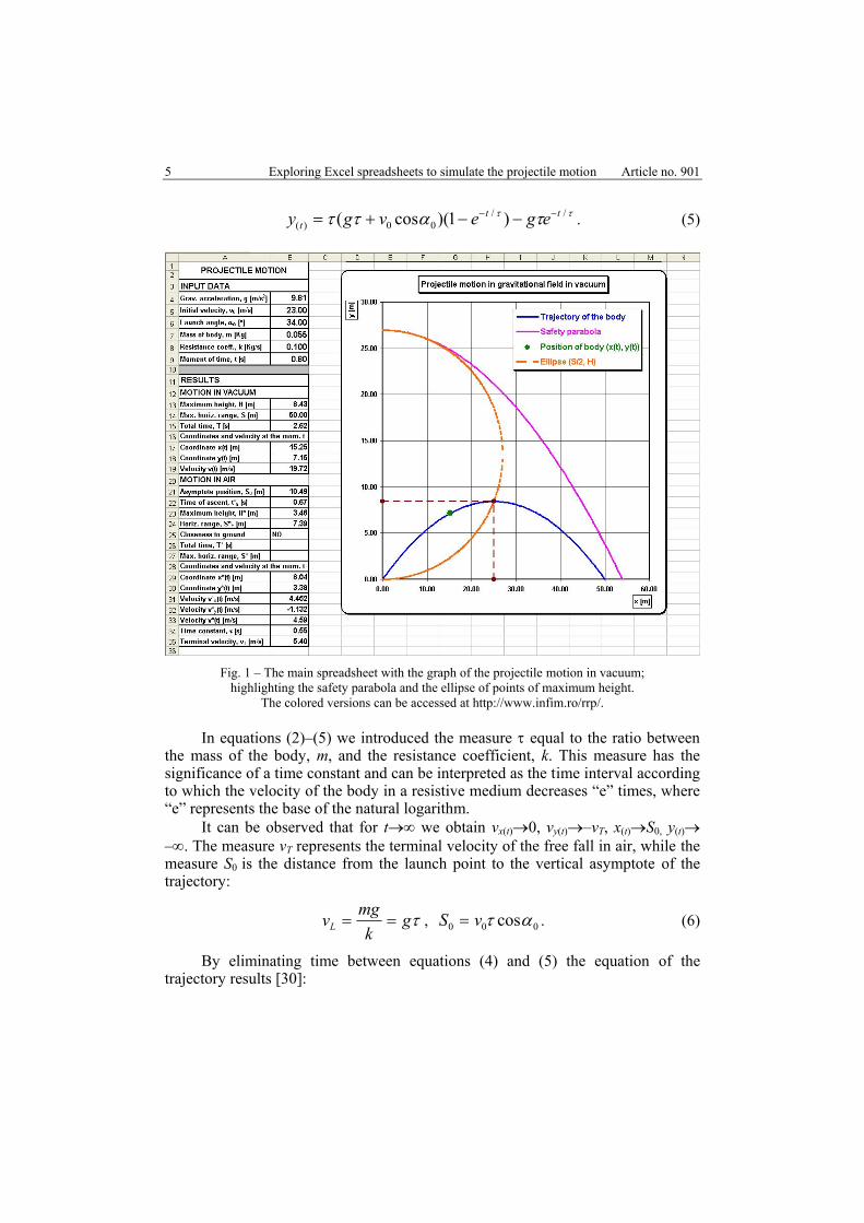
The structure of the tool presented is similar to other tools described by the authors who explore the facilities of Excel spreadsheets in the process of teaching and learning of Physics [27, 28]. The main spreadsheet comprises the sections “Input data” and “Results”, together with the area of the graphs associated. Fig. 1 renders the main spreadsheet with the graph of the projectile motion in vacuum placed next to the input data.


The section “Input data” comprises the domain A3:B9 where the following measures are introduced: gravitational acceleration, g, in cell B4, the initial velocity of the body, v0, in cell B5, the launch angle, α0, in cell B6, the mass of the body, m, in cell B7, the coefficient of resistance, k, in cell B8, and the moment of time t in cell B9.

The section “Results” comprises the domain A11:B35 with two sub-sections, the former for the motion of the body in vacuum and the latter for the motion of the body in air. In the first subsection we calculate the maximum height reached by the body, H, in cell B13, the maximum horizontal range, S, in cell B14, the total time of motion, T, in cell B15. Also, in this subsection, in cells B17, B18 and B19 we calculate the Cartesian coordinates x, y and the velocity v of the body at the moment of time t specified in the input data. In the second subsection we calculate the position of the trajectory asymptote, S0, in cell B21, the time of ascent until the maximum height, t*a, in cell B22, the maximum height reached in air, H*, in cell B23 and the horizontal range corresponding to the maximum height, S*H, in cell B24. Cells B25, B26 and B27 are reserved for the approximate determination of the time of flight, T*, and the maximum horizontal range in air, S*. In cells B29-B33 we calculate the position and the velocity of the body in air at the moment of time specified in the input data. The position is determined by the Cartesian coordinates x*, y* and for the velocity we calculate the components on horizontal and vertical, v*x, v*y, and its magnitude, v*. In cell B34 we calculate the time constant, τ, determined by the mass of the body and the resistance coefficient, while in cell B35 we calculate the terminal velocity of the body in free fall, vT. The measures that appear in the spreadsheet are expressed in S.I. units.

The simple relations presented in introductory physics courses have been used to calculate the measures from the section corresponding to the motion in vacuum [29].

To calculate the measures from the section corresponding to the motion in air, we have used the relations obtained when solving the equation of motion with a drag force linear in the speed:

vkgm

dtvdm rrr

−= . (1)

Taking into account the initial conditions, namely at t = 0, we have x = 0, y = 0, vx = v0cosα0 and vy = v0sinα0, the following results are obtained [11]:

• The velocities for horizontal and vertical directions in relation to time

τα /

00)( )cos( ttx evv −= (2)

τατ τ gevgv tty −+= − /

00)( )sin( . (3) • The Cartesian coordinates x and y in relation to time

)1)(cos( /00)(

τατ tt evx −−= (4)


ττ ταττ //

00)( )1)(cos( ttt egevgy −− −−+= . (5)

Fig. 1 – The main spreadsheet with the graph of the projectile motion in vacuum;

highlighting the safety parabola and the ellipse of points of maximum height. The colored versions can be accessed at http://www.infim.ro/rrp/.

In equations (2)–(5) we introduced the measure τ equal to the ratio between the mass of the body, m, and the resistance coefficient, k. This measure has the significance of a time constant and can be interpreted as the time interval according to which the velocity of the body in a resistive medium decreases “e” times, where “e” represents the base of the natural logarithm.

It can be observed that for t→∞ we obtain vx(t)→0, vy(t)→–vT, x(t)→S0, y(t)→ –∞. The measure vT represents the terminal velocity of the free fall in air, while the measure S0 is the distance from the launch point to the vertical asymptote of the trajectory:

τg

kmgvL == , 000 cosατvS = . (6)

By eliminating time between equations (4) and (5) the equation of the trajectory results [30]:


2( ) 0

0 0 0 0

tg ln 1cos cosxx xy x g

v vα τ

τ α τ α

= + + −

.

(7)

The time of ascent at maximum height, ta, is obtained by making the vertical velocity, vy(t), equal to zero, given by relation (3) and solving in relation to t the algebraic equation obtained. With the expression obtained for the time of ascent, using equations (4) and (5), results the horizontal range corresponding to the maximum height and, respectively, the maximum height reached by the body.

As done in other papers [28], for an easier track of the calculations in Excel, we have named the cells with input data and results. For example, cells B4, B5, B6, B7, B8 and B9 where the input data are introduced have been named Acceleration_G, Velocity_0, Angle_0, Mass, Coefficient_K, and respectively Time. Cell B34 where the time constant τ was calculated, has been named Constant_T. With the previous cell names, using equation (4), we have written the Excel formula to calculate the coordinate x* at the moment t in cell B29:

“=Velocity_0*Constant_T*COS(RADIANS(Angle_0))*(1–EXP(–Time/Constant_T))”.

Analogously, we have written the formulas to calculate the other measures from the section Results. Thus, to calculate coordinate y* in cell B30 we have written in Excel equation (5), to calculate the velocity of the body on the axes x and y in cells B31, B32, equations (2) and (3) etc.

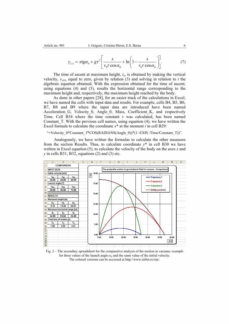
Fig. 2 – The secondary spreadsheet for the comparative analysis of the motion in vacuum; example

for three values of the launch angle α0 and the same value of the initial velocity. The colored versions can be accessed at http://www.infim.ro/rrp/.


The spreadsheet, with its facilities, allows the application of an elementary method to approximately determine the time of flight and the maximum horizontal range in air, and this will be presented below.

The time of flight represents the interval comprised between t = 0 and the moment when the vertical coordinate y(t) becomes equal to zero again. However, from a practical point of view, considering that the object can no longer be considered point mass, the exact condition y(t) = 0 can be replaced with an approximate one of the type y(t) < ε, y(t) > 0. The value of the distance ε is established according to the data of the problem, practically, a value of ε can be set with the same measure as the size of the object. For example, ε = 0.10 m, represents a reasonable value if the object launched is a tennis ball with a diameter of approximately 6.5–7.0 cm. Since the condition y(t) < ε is met around the value t = 0, it is necessary to supplement this relation with a restriction on the moment t to determine the time of flight. As a supplementary condition we can impose that the time t be bigger than the time of ascent, ta. Thus results that the time of flight can be determined from the following conditions:

ε<)(ty , att > . (8)

To explore relations (8), in the spreadsheet we have named cells B22, B25, B29 and B30 as Time_AA, Closeness_G, Coordinate_XA, Coordinate_YA and we have written the following Excel formulas: • In cell B25:

“=IF(AND(ABS(Coordinate_YA)<0.10;Time>Time_AA);"YES";"NO")”; • In cell B26:

“=IF(Closeness_G="YES";Time;" ")”; • In cell B27:

“=IF(Closeness_G="YES";Coordinate_XA;" ")”. Consequently, applying the approximate process of determining the time of

flight and the maximum horizontal range implies modifying the moment of time in cell B9 until the message YES is displayed in cell B25. In this case, the value of the time of flight, T*, in cell B26, is equal to the value of the moment of time from cell B9, and the maximum horizontal range, S*, in cell B27, is equal to the coordinate x*(t) from cell B29. Several attempts are sufficient to determine the two parameters if we simultaneously track the motion of the body on the trajectory in the associated graph.

The graph for the motion of the body in vacuum, rendered in Fig. 1, overlaps the trajectory of the body, the safety parabola and the ellipse of the points of


maximum height for the input data. The parabolic trajectory of the body is rendered in blue, the safety parabola in pink, and the ellipse of the points of maximum height is presented as a dotted orange line. The brown dotted lines highlight the maximum height and the corresponding horizontal range. By modifying the input data, the effect on the curves presented can be observed. If the initial velocity is maintained constant and the launch angle modified, only the trajectory is changed inside the domain framed by the axes x, y and the safety parabola. It is verified that the safety parabola represents the envelope of the family of trajectories for a certain value of the initial velocity. For α0 = 45° the optimum launch angle is obtained for which the total horizontal range becomes maximum. In this case, the landing point is at the intersection between the axis x, trajectory and the safety parabola. Furthermore, it can be observed how the point of maximum height travels along the orange ellipse as the launch angle is modified. The position of the body at a given moment in time is rendered by a green dot on the trajectory. Modifying the value of the moment of time in the input data, we can track the motion of the body on the trajectory.

In a secondary spreadsheet we can simultaneously analyze, for the motion in vacuum, the difference between various trajectories and the safety parabolas associated when changing the input data. Figure 2 presents this secondary spreadsheet where three different sets of values can be introduced in the input data. The initial velocities are introduced in cells A6, B6, C6 and the launch angles in cells A9, B9, C9. The analytic results are displayed in the domain A11:C20. The maximum height is calculated in cells A14, B14, C14, the maximum horizontal range in cells A17, B17, C17, while the total time of motion in cells A20, B20, C20. The graph in Fig. 2 overlaps the trajectories and the safety parabolas corresponding to the three sets of input data. We have used for the trajectories the colors blue, red and green, in this order. In the example presented in the figure we kept the same value for the initial velocity, v0 = 23 m/s, as in Fig. 1, but we considered three different values for the launch angle. In this case, for the three trajectories, we have the same safety parabola rendered in the figure as the brown curve. The trajectory rendered in red for α02 = 45° emphasizes the optimum launch angle. The trajectories rendered in blue and green, for α01 = 20°, respectively, α03 = 70° show that, for values complementary to 90° of the launch angle, the same landing point is obtained. We can maintain the launch angle at the same value and modify the initial velocity to observe a new graphic effect, or consider different values for the initial velocities and the launch angles.

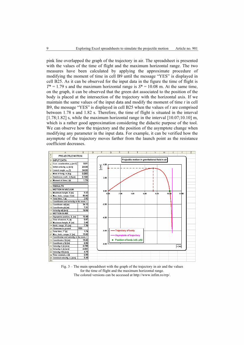
Figure 3 presents the main spreadsheet with the graph of the trajectory in air described by equation (7) and rendered by the red curve. Unlike the motion in vacuum, an asymmetry of the trajectory can be observed in relation to the vertical line crossing the point of maximum height. The vertical asymptote rendered by the


pink line overlapped the graph of the trajectory in air. The spreadsheet is presented with the values of the time of flight and the maximum horizontal range. The two measures have been calculated by applying the approximate procedure of modifying the moment of time in cell B9 until the message “YES” is displayed in cell B25. As it can be observed for the input data in the figure the time of flight is T* = 1.79 s and the maximum horizontal range is S* = 10.08 m. At the same time, on the graph, it can be observed that the green dot associated to the position of the body is placed at the intersection of the trajectory with the horizontal axis. If we maintain the same values of the input data and modify the moment of time t in cell B9, the message “YES” is displayed in cell B25 when the values of t are comprised between 1.78 s and 1.82 s. Therefore, the time of flight is situated in the interval [1.78;1.82] s, while the maximum horizontal range in the interval [10.07;10.10] m, which is a rather good approximation considering the didactic purpose of the tool. We can observe how the trajectory and the position of the asymptote change when modifying any parameter in the input data. For example, it can be verified how the asymptote of the trajectory moves farther from the launch point as the resistance coefficient decreases.

Fig. 3 – The main spreadsheet with the graph of the trajectory in air and the values

for the time of flight and the maximum horizontal range. The colored versions can be accessed at http://www.infim.ro/rrp/.


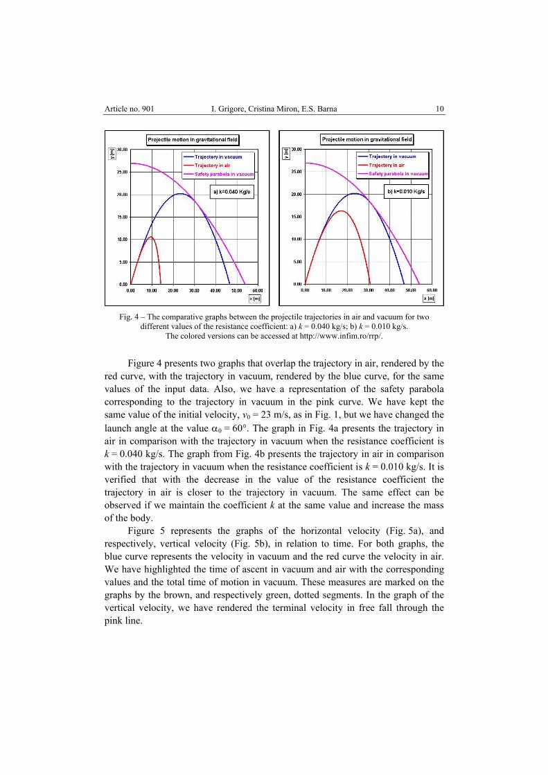
Fig. 4 – The comparative graphs between the projectile trajectories in air and vacuum for two

different values of the resistance coefficient: a) k = 0.040 kg/s; b) k = 0.010 kg/s. The colored versions can be accessed at http://www.infim.ro/rrp/.

Figure 4 presents two graphs that overlap the trajectory in air, rendered by the red curve, with the trajectory in vacuum, rendered by the blue curve, for the same values of the input data. Also, we have a representation of the safety parabola corresponding to the trajectory in vacuum in the pink curve. We have kept the same value of the initial velocity, v0 = 23 m/s, as in Fig. 1, but we have changed the launch angle at the value α0 = 60°. The graph in Fig. 4a presents the trajectory in air in comparison with the trajectory in vacuum when the resistance coefficient is k = 0.040 kg/s. The graph from Fig. 4b presents the trajectory in air in comparison with the trajectory in vacuum when the resistance coefficient is k = 0.010 kg/s. It is verified that with the decrease in the value of the resistance coefficient the trajectory in air is closer to the trajectory in vacuum. The same effect can be observed if we maintain the coefficient k at the same value and increase the mass of the body.

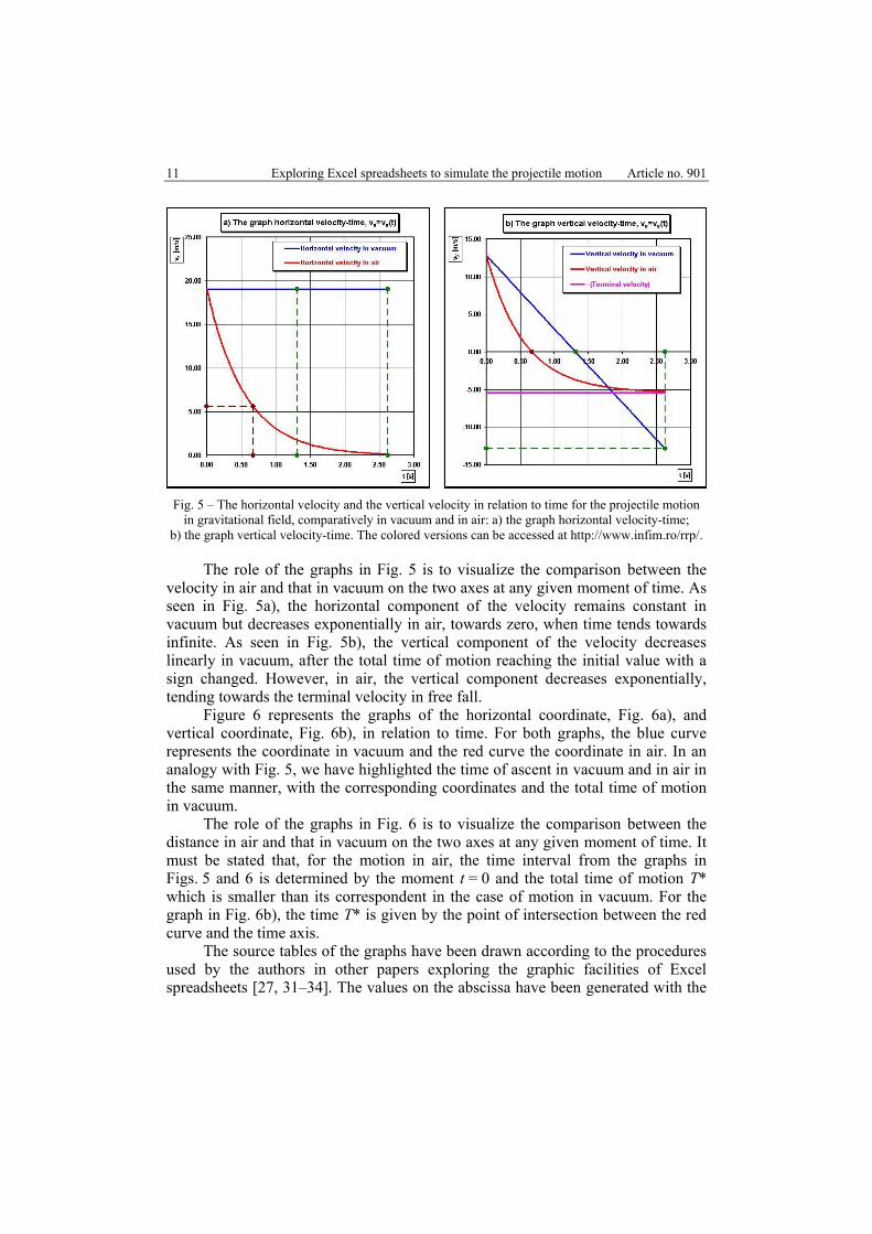
Figure 5 represents the graphs of the horizontal velocity (Fig. 5a), and respectively, vertical velocity (Fig. 5b), in relation to time. For both graphs, the blue curve represents the velocity in vacuum and the red curve the velocity in air. We have highlighted the time of ascent in vacuum and air with the corresponding values and the total time of motion in vacuum. These measures are marked on the graphs by the brown, and respectively green, dotted segments. In the graph of the vertical velocity, we have rendered the terminal velocity in free fall through the pink line.


Fig. 5 – The horizontal velocity and the vertical velocity in relation to time for the projectile motion

in gravitational field, comparatively in vacuum and in air: a) the graph horizontal velocity-time; b) the graph vertical velocity-time. The colored versions can be accessed at http://www.infim.ro/rrp/.

The role of the graphs in Fig. 5 is to visualize the comparison between the velocity in air and that in vacuum on the two axes at any given moment of time. As seen in Fig. 5a), the horizontal component of the velocity remains constant in vacuum but decreases exponentially in air, towards zero, when time tends towards infinite. As seen in Fig. 5b), the vertical component of the velocity decreases linearly in vacuum, after the total time of motion reaching the initial value with a sign changed. However, in air, the vertical component decreases exponentially, tending towards the terminal velocity in free fall.

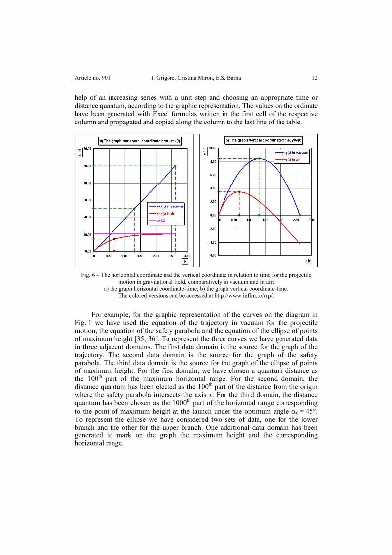
Figure 6 represents the graphs of the horizontal coordinate, Fig. 6a), and vertical coordinate, Fig. 6b), in relation to time. For both graphs, the blue curve represents the coordinate in vacuum and the red curve the coordinate in air. In an analogy with Fig. 5, we have highlighted the time of ascent in vacuum and in air in the same manner, with the corresponding coordinates and the total time of motion in vacuum.

The role of the graphs in Fig. 6 is to visualize the comparison between the distance in air and that in vacuum on the two axes at any given moment of time. It must be stated that, for the motion in air, the time interval from the graphs in Figs. 5 and 6 is determined by the moment t = 0 and the total time of motion T* which is smaller than its correspondent in the case of motion in vacuum. For the graph in Fig. 6b), the time T* is given by the point of intersection between the red curve and the time axis.

The source tables of the graphs have been drawn according to the procedures used by the authors in other papers exploring the graphic facilities of Excel spreadsheets [27, 31–34]. The values on the abscissa have been generated with the


help of an increasing series with a unit step and choosing an appropriate time or distance quantum, according to the graphic representation. The values on the ordinate have been generated with Excel formulas written in the first cell of the respective column and propagated and copied along the column to the last line of the table.

Fig. 6 – The horizontal coordinate and the vertical coordinate in relation to time for the projectile

motion in gravitational field, comparatively in vacuum and in air: a) the graph horizontal coordinate-time; b) the graph vertical coordinate-time.

The colored versions can be accessed at http://www.infim.ro/rrp/.

For example, for the graphic representation of the curves on the diagram in Fig. 1 we have used the equation of the trajectory in vacuum for the projectile motion, the equation of the safety parabola and the equation of the ellipse of points of maximum height [35, 36]. To represent the three curves we have generated data in three adjacent domains. The first data domain is the source for the graph of the trajectory. The second data domain is the source for the graph of the safety parabola. The third data domain is the source for the graph of the ellipse of points of maximum height. For the first domain, we have chosen a quantum distance as the 100th part of the maximum horizontal range. For the second domain, the distance quantum has been elected as the 100th part of the distance from the origin where the safety parabola intersects the axis x. For the third domain, the distance quantum has been chosen as the 1000th part of the horizontal range corresponding to the point of maximum height at the launch under the optimum angle α0 = 45°. To represent the ellipse we have considered two sets of data, one for the lower branch and the other for the upper branch. One additional data domain has been generated to mark on the graph the maximum height and the corresponding horizontal range.


In the same way, the source tables have been drawn for the other graphs. Any of the graphs presented can be placed next to the input data with the option “Freeze panel”. Thus, we have the opportunity to follow the graphical feedback to each parameter change in the input data.

3. CONCLUSIONS

The ability to model, with the help of the tool presented, simple phenomena from real life, like throwing a stone or a tennis ball, can stimulate students’ motivation to study Physics. The results obtained, in both analytical and graphical form, can help students clarify the issues related to the motion in Earth’s constant gravitational field, taking into account the resistance of the medium. With the rapid graphical feedback to input data change, students can better understand the influence of various measures, such as the mass of the body or the resistance coefficient on the trajectory of the motion. The comparative presentation of the motion in vacuum and in air for the same input data can be beneficial for students as they notice the limits of a physical model. Thus, it can be seen under which conditions the trajectory in air comes close to the trajectory in vacuum. Also, a number of concepts such as the safety parabola or the terminal velocity can be more easily integrated when studying motion in the gravitational field. By simulating the motion and viewing the graphs of velocities and horizontal and vertical coordinates, the aspects concerning the motion in two dimensions can be more easily clarified.

This paper continues the authors’ effort to develop interactive teaching tools with spreadsheet that address the motion in the gravitational field, particularly in a resistive medium [31]. While students with poor results will use spreadsheets like “black boxes”, with inputs and outputs, the endowed students can create similar spreadsheets, suitable for solving Physics problems. Teachers are the ones to decide between the “black box” type of approach or asking students to build spreadsheets with various destinations [37]. The tool can be a starting point for solving more difficult problems concerning the projectile motion in the gravitational field where other aspects are considered.

Acknowledgements. I. Grigore was supported by the strategic grant POSDRU/159/1.5/S/ 137750, “Project Doctoral and Postdoctoral programs support for increased competitiveness in Exact Sciences research”cofinanced by the European Social Found within the Sectorial Operational Program Human Resources Development 2007–2013.

REFERENCES

1. C.W. Groetsch, Am. Math. Mon. 103, 7, 546-551 (1996). 2. C.W. Groetsch, B. Cipra, Math. Mag. 70, 4, 273-280 (1997). 3. N.P. Linthorne, J. Sport. Sci. 19, 359-372 (2001).


4. C. White, Projectile Dynamics in Sport: Principles and Applications, Taylor & Francis, Engelska, 2011.

5. P.A. Karkantzakos, Journal of Engineering Science and Technology Review 2, 1, 76-81 (2009). 6. E.W. Packel, D.S. Yuen, Coll. Math. J. 35, 5, 337-350 (2004). 7. R.D.H. Warburton, J. Wang, Am. J. Phys. 72, 11, 1404-1407 (2004). 8. S.M. Stewart, Journal of Engineering Science and Technology Review 4, 1, 32-34 (2011). 9. D.A. Morales, Can. J. Phys. 83, 1, 67-83 (2005). 10. R. Kantrowitz, M.M. Neumann, Optimal Angles for Launching Projectiles: Lagrange vs. Cas,

Canad. Appl. Math. Quart. 16, 3, 279-299 (2008). 11. S.M. Stewart, Eur. J. Phys. 33, 149-166 (2011). 12. H. Hu, Y.P. Zhao, Y.J. Guo, M.Y. Zheng, Acta. Mech. 223, 2, 441-447 (2012). 13. H. Hernandez-Saldana, Eur. J. Phys. 31, 6, 1319-1329 (2010). 14. D.A. Morales, Can. J. Phys. 89, 12, 1233-1250 (2011). 15. R.C. Bernardo, J.P. Esguerra, J.D. Vallejos, J.J. Canda, Eur. J. Phys. 36, 2, Article Number:

025016 (2015). 16. P.S. Chudinov, V.A. Eltyshev, Y.A. Barykin, Lat. Am. J. Phys. Educ. 7, 3, 345-349 (2013). 17. C.H. Belgacem, Eur. J. Phys. 35, 5, Article Number: 055025 (2014). 18. W.W.Hackborn, Am. Math. Mon. 115, 9, 813-819 (2008). 19. R.D.H. Warburton, J. Wong, J. Burgdörfer, J. Service Science & Management 3, 98-105 (2010). 20. C. Das, D. Roy, Resonance 19, 5, 446-465 (2014). 21. A. Verma, A. Desai, S. Mittal, J. Fluid. Struct. 41, 89-98 (2013). 22. V.R. Morrison, Electronic Journal of Classical Mechanics and Relativity, Mount Allison

University, 1-12 (2005). 23. G. Robinson, I. Robinson, Phys. Scripta. 88, 1, Article Number: 018101 (2013). 24. D. Ibrahim, Procedia Soc. Behav. Sci. 1, 309-312 (2009). 25. J. Benacka, Spreadsheets in Education (eJSiE) 3, 2, Article 3 (2009). 26. V.M. Spathopoulos, Comput. Appl. Eng. Educ. 19, 3, 508-513 (2011). 27. I. Grigore, E.S. Barna, Spreadsheets used for simulating composition of the Perpendicular

Harmonic Oscillations, Proceedings of The 10th International Scientific Conference eLearning and Software for Education 2, 217-224 (2014).

28. I. Grigore, I., C. Miron, E.S. Barna, Rom. Rep. Phys. 67, 2, 716-732 (2015). 29. D. Halliday, R. Resnick, J. Walker, Fundamentals of Physics, John Wiley & Sons Inc., 2013. 30. R. Borghi, Eur. J. Phys. 34, 2, 1-15 (2013). 31. I. Grigore, C. Miron, E.S. Barna, Using Excel spreadsheets in the study of motion on an Inclined

Plane in a Resistive Medium, Proceedings of The 11th International Scientific Conference eLearning and Software for Education 3, 483-490 (2015).

32. E.I. Butikov, Eur. J. Phys. 24, L5-L9 (2003). 33. S.K. Foong, C.C. Lim, L. Kuppan, Phys. Educ. 44, 3, 258-263 (2009). 34. K.F. Lim, Newsletter: Using computer in Chemical Education, Spring, 2003, pp. 1-14.

exploring excel spreadsheets to … excel spreadsheets to simulate the ... spreadsheets to simulate...

Documents