exploring fermentation rate in beer and hard cider brewing

EXPLORING FERMENTATION RATE IN BEER AND HARD CIDERBREWING

A thesis presented to the faculty of the Graduate School ofWestern Carolina University in partial fulfillment of the requirements

for the degree of Master of Science in Applied Mathematics

By

Jamie Leigh Rowell

Director: Dr. John Wagaman, Mathematics

Committee Member: Dr. Mark Budden, MathematicsCommittee Member: Dr. Sean O’Connell, Biology

April 9, 2015

iiACKNOWLEDGEMENTS

The full list of people to whom I am forever indebted and grateful to is far too vast to list

here; in short, it has taken a village. To my precious niece and nephew, Annilynn and Ross, thank

you for filling my life with such love and happiness. To my family- Mom, Dad, Brandon, and

Erica: It has taken the combined effort of all four of you to get me here today. Thank you for the

love, laughter, and support you have all given me.

Endless thanks are owed to my thesis advisor, Dr. John Wagaman, for his constant support,

advice, and guidance throughout my time at Western. Another thank you is owed to Dr. Wagaman

for his generosity and financial investment in providing me with many materials necessary for this

study. I would also like to extend thanks my committee members. Dr. Mark Budden and Dr. Sean

O’Connell for their support, ideas, and feedback throughout this process. A special thanks is owed

to Dr. Budden for his vast knowledge of all things math and beer, for his generosity in providing

me with the beer used in this study, and for the support he has given me not only on my thesis, but

throughout my time at Western. Another special thanks is owed to Dr. O’Connell for his generosity

in providing me with all of the materials necessary for data collection, from pipettes to zinc sulfate,

and for offering his time to teach me how to collect beer data. Without the dedication and guidance

of my advisor and committee members this work would have, quite literally, not been possible.

To the other 23 of the dream-team, Nic Stolt and Aaron Rapp, thank you for the trivia

answers, Sunday night TV shows, tomahawk chops, and invaluable friendship. Endless thanks is

also owed to the rest of my math-bros for their support and friendship: Josh Hiller, Cole Drawdy,

Kasey Jones, and Adam Schrum.

iiiCONTENTS

Page

LIST OF FIGURES . . . . . . . . . . . . . . . . . . . . . . . . . . . . . . . . . . . . . . iv

ABSTRACT . . . . . . . . . . . . . . . . . . . . . . . . . . . . . . . . . . . . . . . . . . vi

1 INTRODUCTION . . . . . . . . . . . . . . . . . . . . . . . . . . . . . . . . . . . . . 1

A Brief Introduction to Homebrewing . . . . . . . . . . . . . . . . . . . . . . . . . . . 1The Homebrewing Process . . . . . . . . . . . . . . . . . . . . . . . . . . . . . . . . . 2The Importance of Fermentation . . . . . . . . . . . . . . . . . . . . . . . . . . . . . . 4Measuring Fermentation Rate . . . . . . . . . . . . . . . . . . . . . . . . . . . . . . . . 6

2 METHODS AND MATERIALS . . . . . . . . . . . . . . . . . . . . . . . . . . . . . 8

Yeast Strains . . . . . . . . . . . . . . . . . . . . . . . . . . . . . . . . . . . . . . . . . 8Sample Preparation . . . . . . . . . . . . . . . . . . . . . . . . . . . . . . . . . . . . . 8Sample Collection . . . . . . . . . . . . . . . . . . . . . . . . . . . . . . . . . . . . . . 10

3 DATA ANALYSIS . . . . . . . . . . . . . . . . . . . . . . . . . . . . . . . . . . . . . 11

Cider1 . . . . . . . . . . . . . . . . . . . . . . . . . . . . . . . . . . . . . . . . . . . . 11IPA38 . . . . . . . . . . . . . . . . . . . . . . . . . . . . . . . . . . . . . . . . . . . . 23IPA39 . . . . . . . . . . . . . . . . . . . . . . . . . . . . . . . . . . . . . . . . . . . . 28Cider2 . . . . . . . . . . . . . . . . . . . . . . . . . . . . . . . . . . . . . . . . . . . . 33

4 CONCLUSIONS . . . . . . . . . . . . . . . . . . . . . . . . . . . . . . . . . . . . . . 45

REFERENCES . . . . . . . . . . . . . . . . . . . . . . . . . . . . . . . . . . . . . . . . . 47

APPENDICES . . . . . . . . . . . . . . . . . . . . . . . . . . . . . . . . . . . . . . . . . 49Appendix 1: R code for Cider1 . . . . . . . . . . . . . . . . . . . . . . . . . . . . . . . 49Appendix 2: R code for IPA38 . . . . . . . . . . . . . . . . . . . . . . . . . . . . . . . 53Appendix 3: R code for IPA39 . . . . . . . . . . . . . . . . . . . . . . . . . . . . . . . 55Appendix 4: R code for Cider2 . . . . . . . . . . . . . . . . . . . . . . . . . . . . . . . 57

ivLIST OF FIGURES

1 Cider1: A plot of specific gravity against time (hours), with least squares regres-sion line (black). Symbols: ◦ ≡ vessel 1 (red) and4 ≡ vessel 2 (orange), both ofwhich received no yeast nutrient. +≡ vessel 3 (yellow) and×≡ vessel 4 (green),both of which received half the recommended amount of yeast nutrient. �≡ vessel5 (blue) and ∇ ≡ vessel 6 (purple), both of which received the full recommendedamount of yeast nutrient. . . . . . . . . . . . . . . . . . . . . . . . . . . . . . . . 12

2 Cider1: Plots of log-likelihood against λ for proposed Box-Cox transformation . . 153 Cider1: Pre/Post Box-Cox Transformation . . . . . . . . . . . . . . . . . . . . . . 164 Cider1: Grouping replicates within each treatment level . . . . . . . . . . . . . . . 175 Cider1: Grouping replicates within each treatment level . . . . . . . . . . . . . . 196 Cider1: Modeling Mean Specific Gravity . . . . . . . . . . . . . . . . . . . . . . 217 IPA38: A plot of specific gravity against time (hours). Symbols: ◦ ≡ vessel 1

(red), 4 ≡ vessel 2 (orange), + ≡ vessel 3 (yellow) and × ≡ vessel 4 (green),� ≡ vessel 5 (blue) and ∇ ≡ is vessel 6 (purple), where vessels 1-6 were filled inchronological order, with vessel 1 being filled first and vessel 6 being filled last. . 23

8 IPA38: Modeling Mean Specific Gravity . . . . . . . . . . . . . . . . . . . . . . . 249 IPA39: A plot of specific gravity against time (hours), where a refractometer was

used to measure specific gravity. Symbols: ◦ ≡ vessel 1 (red), 4 ≡ vessel 2(orange), +≡ vessel 3 (yellow) and×≡ vessel 4 (green), �≡ vessel 5 (blue) and∇≡ is vessel 6 (purple), where vessels 1-6 were filled in chronological order, withvessel 1 being filled first and vessel 6 being filled last. . . . . . . . . . . . . . . . 28

10 IPA39: A plot of specific gravity against time (hours), where a hydrometer wasused to measure specific gravity. Symbols: ◦ ≡ vessel 1 (red), 4 ≡ vessel 2(orange), +≡ vessel 3 (yellow) and×≡ vessel 4 (green), �≡ vessel 5 (blue) and∇≡ is vessel 6 (purple), where vessels 1-6 were filled in chronological order, withvessel 1 being filled first and vessel 6 being filled last. . . . . . . . . . . . . . . . 29

11 IPA39: Hydrometer Specific Gravity vs. Refractometer Specific Gravity . . . . . . 3112 Cider2: A plot of specific gravity against time (hours).

Symbols: ◦ ≡ vessel 1 (green), 4≡ vessel 2 (green), both of which were in thecontrol treatment, and as such, received no yeast nutrient or zinc.+ ≡ vessel 3 (orange) and× ≡ vessel 4 (orange), both of which received half therecommended amount of yeast nutrient.� ≡ vessel 5 (red) and ∇ ≡ vessel 6 (red), both of which received the full recom-mended amount of yeast nutrient.� ≡ vessel 7 (cyan) andC≡ vessel 8 (cyan), both of which received the smalleramount of zinc.+�≡ vessel 9 (blue) and

⊕≡ vessel 10 (blue), both of which received the larger

amount of zinc.C≡ vessel 11 (purple) and �≡ vessel 12 (purple), both of which received half therecommended amount of yeast nutrient and the smaller amount of zinc. . . . . . . 34

13 Cider2: Specific Gravity Differences versus Time . . . . . . . . . . . . . . . . . . 37

v14 Cider2: Mean-Corrected Specific Gravity Differences vs Time (post hour 100)

Symbols: ◦ ≡ vessel 1 (green), 4≡ vessel 2 (green), + ≡ vessel 3 (orange) and× ≡ vessel 4 (orange), � ≡ vessel 5 (red) and ∇ ≡ vessel 6 (red), � ≡ vessel 7(cyan) andC≡ vessel 8 (cyan), +�≡ vessel 9 (blue) and

⊕≡ vessel 10 (blue), C≡

vessel 11 (purple) and �≡ vessel 12 (purple). . . . . . . . . . . . . . . . . . . . . 3915 Cider2: Hydrometer versus Refractometer . . . . . . . . . . . . . . . . . . . . . . 43

vi

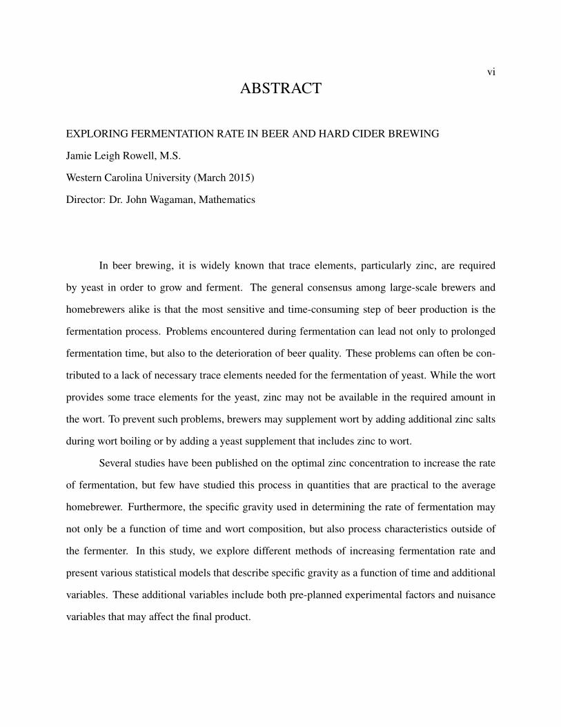
ABSTRACT

EXPLORING FERMENTATION RATE IN BEER AND HARD CIDER BREWING

Jamie Leigh Rowell, M.S.

Western Carolina University (March 2015)

Director: Dr. John Wagaman, Mathematics

In beer brewing, it is widely known that trace elements, particularly zinc, are required

by yeast in order to grow and ferment. The general consensus among large-scale brewers and

homebrewers alike is that the most sensitive and time-consuming step of beer production is the

fermentation process. Problems encountered during fermentation can lead not only to prolonged

fermentation time, but also to the deterioration of beer quality. These problems can often be con-

tributed to a lack of necessary trace elements needed for the fermentation of yeast. While the wort

provides some trace elements for the yeast, zinc may not be available in the required amount in

the wort. To prevent such problems, brewers may supplement wort by adding additional zinc salts

during wort boiling or by adding a yeast supplement that includes zinc to wort.

Several studies have been published on the optimal zinc concentration to increase the rate

of fermentation, but few have studied this process in quantities that are practical to the average

homebrewer. Furthermore, the specific gravity used in determining the rate of fermentation may

not only be a function of time and wort composition, but also process characteristics outside of

the fermenter. In this study, we explore different methods of increasing fermentation rate and

present various statistical models that describe specific gravity as a function of time and additional

variables. These additional variables include both pre-planned experimental factors and nuisance

variables that may affect the final product.

1

1 INTRODUCTION

A Brief Introduction to Homebrewing

People began brewing beer in their homes over 6,000 years ago [Papazian, 2003]. In the

colonial period and up to the middle of the 19th century, homebrewed hard cider was one of

the most popular beverages in America [Pittet, 2011]. While homebrewing has been around for

thousands of years, it has seen a spike in popularity in recent years, which some credit to the

growth of the microbrewing industry. But despite its recent spike in popularity, many people have

never been involved in the homebrewing process. For people who have never participated in the

homebrewing process, a common question directed to homebrewers is “Why homebrew?” Some

common initial assumptions are that people homebrew in an effort to save money or because of a

lack of variety in beers currently on the market. Even if people begin brewing their own beer for

these reasons, they often find that these are not the reasons why they continue homebrewing.

It can, of course, be less expensive to brew beer at home rather than purchasing beer from

commercial retailers. However, after people begin homebrewing they often find that their focus

shifts from the lessened cost of homebrewing to the opportunity that homebrewing presents to

be creative in producing quality, unique brews. With the wide range of brews currently on the

market, it is harder to justify homebrewing on the basis that a desired product cannot be found on

the market today. Though more and more people can enjoy the wide range of beer/cider currently

available, many of these people want to make these products themselves or expand on what is

currently available.

Making beer/cider at home has taken on new meaning in recent years. Homebrewers are

becoming increasingly knowledgeable about brewing and are becoming more innovative and cre-

ative in their brewing practices. Homebrewing has become more than a hobby for many people.

Many homebrewers now place a focus on the replicability of brews, which is indicative of the logi-

2cal and developmental approach to brewing that is used by homebrewers today. Homebrewers and

large-scale (commercial) brewers share a common goal of making the highest quality, most con-

sistent brew in the shortest amount of time for a variety of reasons. One reason, the most obvious

of reasons, is that brewers simply want their brew quickly. Commercial brewers want to get the

product out to the customer as quickly as possible in an effort to achieve the shortest turnaround

time possible, in order to maximize profits (i.e., move product through the fermenters quickly).

Similarly, homebrewers want to have a usable product in the shortest amount of time possible.

Another, more critical, reason that brewers desire a short turnaround time is that this shortens the

amount of time that the brew remains in the fermentation stage, which is the most sensitive step

of the brewing process. When brews remain in the fermentation stage for longer amounts of time,

this increases the likelihood of encountering problems.

The Homebrewing Process

Before brewing begins and before ingredients are purchased, a homebrewer must decide

whether they intend to start from scratch and brew their beer exactly as commercial breweries do,

or to choose the more simplistic route. Unlike commercial breweries, it may not be more cost-

effective for homebrewers to grind or mash their own grains (i.e., all grain brewing). Instead,

homebrewers can choose to avoid these time-consuming steps and use malt extract. Malt extract

is malted barley that has been processed into a malt “soup,” where 70 to 80 percent of the water

is evaporated, leaving a concentrated syrup or further dried to create a powder [Papazian, 2003].

Brewing with malt extract offers an advantage as it does not require as much time and equipment as

all-grain brewing. While there are advantages and disadvantages to both all-grain brewing and malt

extract brewing, the decision of which path to choose ultimately depends on the brewer’s personal

preference. After deciding between the options of starting from scratch or using malt extract, the

homebrewer must gather the required equipment and ingredients that correspond to the particular

3beer or cider they wish to brew. A detailed outline of the required equipment and ingredients

needed for a beginning homebrewer can be found in The Complete Joy of Homebrewing [Papazian,

2003].

Following the acquisition of all required equipment and ingredients, the malt extract (if

used) and other ingredients, including hops (these are added to the brew pot after the boil starts),

will be added to water and brought to a boil in a brew pot to prepare a wort. Wort is a term

used by brewers to describe unfermented beer [Papazian, 2003]. After the wort has boiled for

approximately one hour, it is transferred from the brew pot to the fermenter(s) and cooled. When

the temperature of this mixture is below approximately 75 degrees Fahrenheit, a first measurement

of specific gravity will be taken using a hydrometer or refractometer (this measurement will later

be referred to as the original gravity). A hydrometer is an instrument that measures the density of

a liquid relative to the density of water. This measure of density is known as specific gravity. The

specific gravity of water is exactly 1.000, thus adding dissolvable solids such as sugar to the water

causes the solution to become more dense and the specific gravity rises above 1.000 [Papazian,

2003]. After the original gravity of the wort is measured, the yeast will be added. The addition

of yeast to the wort is often referred to, among brewers, as pitching. After the yeast is pitched,

an airlock will be attached. The airlock is a device that allows carbon dioxide to be released from

the fermenter without allowing air to enter the fermenter. The airlock is approximately half-filled

with water, which will allow fermentation to become a visible process as the gases produced by

fermentation bubble through the airlock.

After the yeast is pitched, the wort is now referred to as beer/cider. This change in reference

occurs due to the fact that the beer/cider has now entered the fermentation stage. The fermentation

stage is the most critical stage of the brewing process. The amount of time that a beer remains in the

fermentation stage varies depending on the style of beer/cider being brewed. Generally, after two

to three days of vigorous fermentation, activity will subside and yeast will become dormant due

to food depletion and alcohol buildup, and fermentation will begin to subside. After fermentation

has ended, the beer/cider will be bottled or kegged and then aged over a period of generally 7-14

4days [Papazian, 2003].

Brewing cider is a decidedly more simple process in comparison to that of beer. Hard cider

is made from apple juice or apple cider, and if the juice or cider is preservative free, there is no need

to boil the juice or cider in a brew pot, although some recipes do call for boiling. Before brewing

begins and before ingredients are purchased, a homebrewer must decide whether they intend to

use unpasteurized or pasteurized apple juice/cider. If the juice/cider is unpasteurized, sulfite can

be added to remove wild yeasts. Before any yeast or yeast supplements are added to the apple

juice/cider, the original gravity will be measured using a hydrometer or refractometer, following

which the yeast and yeast supplements will be added.

The Importance of Fermentation

The general consensus among large-scale brewers and homebrewers alike is that the most

sensitive and time-consuming step of beer production is the fermentation process. Depending on

the style of beer, the fermentation process can last anywhere from ten days (e.g., ales) to several

months (e.g., lagers) [Papazian, 1994]. During this fermentation process, yeast cells reproduce and

disperse themselves throughout the fermenting beer, converting sugars to alcohols, carbon dioxide

and various flavor compounds. After a few days the yeast will have consumed most of its sugar

supply and fermentation will begin to subside.

Yeasts are living microbiological organisms, and as such, they are affected by environmen-

tal factors such as temperature or contamination by wild yeasts or other yeast strains. If the yeast in

a homebrew does not have an environment in which it can thrive, this can lead to problems during

fermentation. Additionally, if there is not an adequate amount of trace elements, particularly zinc,

in the wort this can also potentially lead to problems during fermentation. Problems encountered

during the fermentation process can lead to not only prolonged fermentation time, but also the

deterioration of beer quality.

With the sensitivity of the fermentation stage comes a natural desire to increase the rate of

5fermentation; the shorter amount of time a brew remains in the fermentation stage, the less chance

you have of encountering problems. Given that homebrewers are becoming more innovative in

their brewing, it is natural that they are seeking creative ways to increase the rate of fermentation.

It is known, based on biochemical and microbiological experiments, that yeasts require certain

trace elements in order to grow and ferment [Helin and Slaughter, 1977]. Trace elements that have

been widely studied regarding their essential nature in fermentation are zinc, calcium, manganese,

cobalt, and iron [Maddox and Hough, 1970], [Helin and Slaughter, 1977] [Papazian, 2003]. When

these trace elements are not available in the required amounts, many problems can ensue. Potential

problems include slow fermentation, mutation of yeasts, poor sedimentation, and off-flavors. It has

been conjectured that problems encountered during fermentation can, most often, be contributed to

low zinc concentration of the wort or the yeast [Vecseri-Hegyes et al., 2005]. In an effort to promote

yeast health and prevent off-flavors, many breweries add zinc sulfate, zinc chloride, or Servomyces

to wort [White, 2013]. Servomyces are dead yeast that serve as a nutritional yeast supplement and

work to cut down fermentation time and improve the health and viability of yeast. More recent

findings suggest that preconditioning brewing yeast cells with zinc may be a more effective way

to enhance fermentation performance rather that supplementing wort with zinc [De Nicola and

Walker, 2011].

Commercial brewers have an advantage over homebrewers in that they have the resources

to test wort composition and determine if it is necessary to supplement with additives such as zinc

salts or Servomyces, which can be costly. For homebrewers, testing wort composition may not

be a realistic option, and as a result, it simply may not seem cost-effective enough to supplement

using these types of additives. Similarly, homebrewers may not have the equipment or resources

necessary to precondition brewing yeast cells with zinc. However, one realistic, cost-efficient

method of increasing the speed of fermentation that homebrewers commonly use is the addition

of a commercially prepared yeast nutrient. Yeast nutrient provides a blend of vitamins, minerals,

amino acids, nitrogen compounds, zinc, and trace elements, all of which are necessary for rapid

and complete fermentation [Wyeast Laboratories, 2015]. Wyeast Laboratories Inc. is a worldwide

6leader in the fermentation industry as a producer of yeast cultures and fermentation products.

Wyeast claims that supplementing wort with yeast nutrient will reduce lag time, enhance yeast

viability, and encourage consistent attenuation rates [Wyeast Laboratories, 2015]. Attenuation

is a measure of how much of the sugars were converted into alcohol and carbon dioxide by the

fermentation process.

Another factor that could potentially affect fermentation rate is trub. Trub is the sedi-

ment that collects at the bottom of the fermenter when brewing beer/cider. It is known that the

presence of trub in fermenting wort can affect the fermentation and flavor [Papazian, 2003]. Com-

mercial brewers are careful to remove this trub before even transferring the wort to its fermenter.

Commercial brewers remove this trub by whirlpooling the wort as it is drawn from the brewpot.

Homebrewers, however, may not have the ability to whirlpool the wort while transferring the wort

into the fermenter. In this case, homebrewers must consider the effect that trub may have on the

rate of fermentation. If a homebrewer transfers wort from the brewpot into multiple fermenters,

the amount of trub in each of the fermenters will most likely not be equal. Given that we know that

the presence of trub in the fermenting wort will affect the rate of fermentation, a natural question

arises as to whether the order in which the fermenters are filled affect the rate of fermentation.

Measuring Fermentation Rate

We know that when the fermentation process is near completion, the yeast will go dormant

and either float to the top or sink to the bottom of the fermenter, depending on the strain of yeast.

This process is commonly referred to as flocculation. While the flocculation of yeast is a good

indication that fermentation is nearing completion, we can test the degree of attenuation to confirm

that fermentation has ended. Recall that attenuation is a measure of how much of the sugars in

beer/cider wort is converted by the fermentation process to alcohol and carbon dioxide, and is

indicated by the difference between original gravity and final specific gravity [Papazian, 2003].

7Recall that before the yeast has been pitched, the specific gravity is checked with a hydrometer.

During fermentation, the specific gravity can be re-checked. The specific gravity will decrease over

time since the sugars that were present in the wort will be consumed by yeast during fermentation.

The consumption of sugar by yeast causes the density of the liquid to decrease, which as a result,

lowers the specific gravity. It is common to consider fermentation finished when the hydrometer

readings of specific gravity remain unchanged for 2-3 days [Papazian, 2003].

While hydrometers are the most common tool used to measure the specific gravity of cider

or beer, there are other options. Another tool that can be used to measure specific gravity is called a

refractometer. A refractometer is an instrument that measures the gravity of a solution by measur-

ing the angle at which light passes through the sample. Refractometers are relatively inexpensive,

but they do have one downfall: they are only accurate for original gravity. Refractometers are

affected by the presence of alcohol in a solution, so they do not give accurate readings of specific

gravity after the yeast has been pitched and fermentation begins. However, there are several advan-

tages to using a refractometer in place of a hydrometer. Refractometers require very little volume

of liquid, typically less than 1 mL, whereas hydrometers require a much larger volume of sample:

the hydrometer used in these experiments requires between 75 to 95 mL of sample to read specific

gravity. Taking several specific gravity measurements throughout the fermentation stage could

lead to a waste of a substantial amount of beer/cider, since 355 mL are in a typical bottle of beer so

one beer is used to obtain every 4-5 hydrometer readings. Most refractometers have an automatic

temperature conversion, so samples can be taken directly from the kettle, whereas hydrometers are

temperature dependent. Using a refractometer as opposed to a hydrometer also saves time when

taking measurements of specific gravity. Taking several specific gravity measurements throughout

the fermentation stage may take a substantial amount of time if using a hydrometer, whereas using

a refractometer takes only a few seconds per reading.

8

2 METHODS AND MATERIALS

Multiple experiments were conducted over a period of several months, each with differ-

ent materials and purposes. Below these materials and purposes are described, with the selected

data analyses following in Chapter 3. Several of the earlier experiments served as vehicles for

improving data collection techniques as the author had no experience with homebrewing prior to

this work.

Yeast Strains

Two yeast strains for four different brews have been employed in this study. The four

different brews analyzed in this study are named Cider1, IPA38, IPA39, and Cider2. For Cider1

and Cider2, Red Star pasteur champagne yeast, a yeast strain of Saccharomyces bayanus, was

used. For IPA38 and IPA39, Safale US05, a yeast strain of Saccharomyces cerevisiae, was used.

The naming convention of the different brews is that of a local homebrewer. For instance, IPA38

and IPA39 are so named because they are 38th and 39th beers of India Pale Ale (IPA) style brewed

by him.

Sample Preparation

During sample preparation for Cider1, we were trying to determine how the amount of

yeast nutrient added to cider would affect the fermentation rate. More specifically, we were try-

ing to determine if adding yeast nutrient to cider could increase the rate of fermentation. This

study used six one-gallon vessels of Earthfare Organic Apple Juice where each vessel was given

an equivalent amount of yeast. Fermenting cider samples treated with varying amounts of yeast

nutrient were examined. This experiment was carried out for 432 hours and specific gravity read-

ings were obtained using a refractometer at 0, 45, 250, 288, 339, 387, and 432 hours.

9During sample preparation for IPA38, we were trying to determine whether the order in

which the vessels were filled from the kettle would affect the fermentation rate. In this study, ap-

proximately 12 gallons of wort was initially prepared and half (six gallons) went directly to the

brewer in a 6.5-gallon carboy and the other half was emptied into six one-gallon vessels. The order

of fill was such that one gallon was emptied into vessel 1 followed by one gallon into the carboy.

Next, another gallon was emptied into vessel 2 followed by another (second) gallon into the carboy.

The vessels were continually filled in this manner, so that vessel 1 contained wort near the bottom

of the brew kettle and vessel 6 contained wort near the top of the brew kettle. This experiment was

carried out for 290 hours and specific gravity readings were obtained using a refractometer at 0,

22, 55, 122, 147, 195, 240 and 290 hours.

During sample preparation for IPA39, we were attempting to quantify the error in refrac-

tometer readings in comparison to hydrometer readings over time. The vessels were filled in a

manner similar to that of IPA38, so, in addition to the purpose of error quantification, we sought

to determine whether order of fill was important for fermentation using a larger number of time

observations. This experiment was carried out for 180.5 hours and specific gravity readings were

obtained using both a refractometer and hydrometer at 19, 31, 46, 56, 68, 92, 104, 116, 128.5, 140,

152, 168.5 and 180.5 hours.

During sample preparation for Cider2, we were trying to determine how the amount of

zinc and/or yeast nutrient added to cider would affect the fermentation rate. More specifically, we

wanted to determine whether the addition of zinc sulfate, yeast nutrient, or a combination of zinc

sulfate and yeast nutrient to cider could increase the fermentation rate, and if so, which treatment

would have the greatest effect on fermentation rate. This study used twelve one-gallon vessels

of Earthfare Organic Apple Juice where each vessel was given an equivalent amount of yeast.

Fermenting cider samples treated with varying amounts of zinc sulfate and yeast nutrient were ex-

amined. This experiment was carried out for 369 hours and specific gravity readings were obtained

10using a refractometer and/or hydrometer at 0, 11, 27, 37, 52.33, 61.33, 68, 89.67, 130.33, 149.33,

177.67, 225.67, 273.67, 320.17, and 369 hours.

Sample Collection

Samples of fermenting beer and cider were obtained using an automatic temperature com-

pensating refractometer and/or a hydrometer. Video recordings were also taken prior to the collec-

tion of beer/cider samples to monitor the air lock bubbling for each vessel.

11

3 DATA ANALYSIS

Cider1

Recall that we were using the Cider1 data to determine how the amount of yeast nutrient

added to cider will affect the fermentation rate. More specifically, we were trying to determine

if adding yeast nutrient to cider could increase the rate of fermentation. Wyeast laboratories rec-

ommends using half a teaspoon of yeast nutrient per five gallons of wort. With this in mind,

we constructed three treatment levels for this experiment. In treatment level 1, vessels 1 and 2

received no yeast nutrient, in treatment level 2, vessels 3 and 4 received half the recommended

amount of yeast nutrient, and in treatment level 3, vessels 5 and 6 received the full recommended

amount of yeast nutrient. After the fermentation of Cider1 was complete, we began by graphically

considering our data.

12

Figure 1: Cider1: A plot of specific gravity against time (hours), with least squares regressionline (black). Symbols: ◦ ≡ vessel 1 (red) and 4 ≡ vessel 2 (orange), both of which received noyeast nutrient. + ≡ vessel 3 (yellow) and × ≡ vessel 4 (green), both of which received half therecommended amount of yeast nutrient. � ≡ vessel 5 (blue) and ∇ ≡ vessel 6 (purple), both ofwhich received the full recommended amount of yeast nutrient.

From this plot of specific gravity versus time (hours), we see that the relationship between

these two variables does not appear to be entirely linear. We also notice a large gap in specific

gravity measurements between 50 and 250 hours. Cider1 was brewed immediately prior to a

holiday week and measurements were not taken during this week. It should also be noted that

vessels 2 and 4 experienced increases in specific gravity; generally this is not possible and is due

to the limits of precision of the measurement instruments. Problems encountered with the limited

precision of measurement instruments are not unique to this study and have been addressed in

other studies [Defernez et al., 2007]. While the data may not suggest that the best model is a

linear model, one starting model is a linear mixed-effects model (LME). Mixed-effects models

have gained popularity over the last two decades, in part because of the development of reliable

and efficient software for fitting and analyzing them [Pinheiro and Bates, 2000]. A linear mixed-

effects model is a good starting model for this data since we have repeated measurements on the

13same subject over time (repeated specific gravity readings on each vessel over time).

We wish to determine if the amount of yeast supplement added to wort affects the rate of

fermentation. Since we want to compare the three different treatment levels over time, we will

use fixed effects for the treatment factor and the time factor. The six different vessels represent

samples from the population about which we wish to make inferences, so we use random effects

to model the vessel factor. We model the data as follows:

yi j = β0 +β1ti + τk +b j + εi j (1)

where

• yi j denotes the specific gravity of vessel j at time ti for i = 1, . . . ,7 and j = 1, . . . ,6

• β0 denotes the intercept of the linear model

• β1 denotes the slope of the linear trend effect of specific gravity due to time

• ti denotes the time, in hours, at time point i

• τk denotes the treatment effect due to the yeast nutrient in treatment level k, for k = 1,2,3,

where τ1 = 0 for the control treatment.

• b j denotes the random effect due to vessel j where it is assumed that b j ∼ N(0,σ2b)

• εi j denotes the random error of the observation at time ti for vessel j where it is assumed that

εi j ∼ N(0,σ2ε).

The estimates for the random-effects standard deviations are given by σb = 1.614× 10−7

and σε = 0.005. Recall that σb represents the standard deviation between vessels and σε repre-

sents the standard deviation within vessels. Thus we see that there is far less variability between

vessels compared to within vessels. We note that while the p-value for time was 0, the p-values

for treatment levels 2 and 3 were relatively high, 0.73 and 0.80, respectively. Rather than using

14these results to reduce our model, we reconsider the fact that the relationship between specific

gravity and time did not appear entirely linear, and this fact may contribute to poor model fit and

compromised parameter estimates and p-values.

In an attempt to overcome problems due to nonlinearity, we first consider a transformation

of the response variable, specific gravity (sg), using a Box-Cox procedure [Sheather, 2009]. Box-

Cox transformations are variable transformations that are commonly used to transform a strictly

positive response variable. Two assumptions of linear models are that the response function is

linear and the error terms come from a normal distribution; that is, the residuals come from a

normal distribution with mean 0 and variance σ2ε .

Box-Cox transformations use the method of maximum likelihood to identify the power to

which to response variable should be raised, denoted by λ, in order to correct the skewness in the

distribution of the error terms, as well as correct unequal error variances and nonlinearity of the re-

gression function [Neter et al., 1996]. The unfortunate drawback of using variable transformations

is that the interpretation of the response variable is not as originally measured. Variable transfor-

mations make the model more difficult to interpret and as a result, it is common practice to choose

a value in the neighborhood of λ that makes the power transformation easy to understand [Neter

et al., 1996]. Furthermore, due to the lack of interpretability of the response variable, we will only

use the Box-Cox transformation if it is beneficial. We will attempt a Box-Cox transformation to

transform the response variable, sg, to a new variable, (sg)λ, where the value of λ is estimated

with a Box-Cox procedure using the method of maximum likelihood. Note that Figure 2 provides

plots of the log-likelihood against λ for the Cider1 data.

15

Figure 2: Cider1: Plots of log-likelihood against λ for proposed Box-Cox transformation

The value of λ that maximizes the log-likelihood and the 95% confidence limits are marked

on each plot. The values on the horizontal axis of the right hand plot are restricted so that it is easier

to identify the value of λ that maximizes the log-likelihood, and from Figure 2 we see that this

value is λ≈−130. That is, performing the Box-Cox transformation suggests that the appropriate

transformation for this data results in the following model:

y−130i j = β0 +β1ti + τk +b j + εi j, (2)

We note that λ = −130 does not provide an easily interpretable transformation, but in order to

assess whether performing the Box-Cox transformation was beneficial, we graphically explore and

compare both the original model and the transformed model, in Figure 3.

16

Figure 3: Cider1: Pre/Post Box-Cox Transformation

Comparing the plots of the original data and the transformed data, we observe that the

Box-Cox transformation did not overcome our problems due to nonlinearity.

Given that our attempt at a variable transformation did not prove to be useful, we will

proceed by further graphically exploring our original model. To better determine whether the

treatment effects were significant, we group together the two replicates within each treatment so

there are three panels, one for each of the three treatment levels, which can be seen in Figure 4

17

Figure 4: Cider1: Grouping replicates within each treatment level

Before we continue, we will consider a problem with our original model that we have

not addressed thus far. The goal of model (1) was to determine whether there is a significant

difference in the specific gravity of each vessel at each time point. But realistically, we know

that the specific gravity of each vessel should not be very different at each time point, particularly

at the beginning and end of fermentation. Since the cider in each of the six vessels should be

approximately uniform, each of the vessels should have approximately the same alcohol content,

with some variability due to the initial sugar content of the apple juice in each individual vessel.

Similarly, when the fermentation of the cider nears completion, the specific gravity of each of the

18vessels will begin to plateau to approximately the same final gravity. Thus, we hypothesize that

model (1) may not be as useful in quantifying the effect of yeast nutrient since we are including

specific gravity readings at each time point. More specifically, since the majority of the specific

gravity readings taken for Cider1 are at the beginning and end of fermentation, and very few are in

a range where the differences should be at a maximum, we acknowledge that model (1) may not

be appropriate for answering our overarching question (with this data).

In order to determine whether the amount of yeast supplement added to each vessel has an

effect on fermentation rate we may want to consider the time point at which the specific gravity

of each individual vessel begins to plateau to this final gravity. In this case, the final gravity of

each vessel was 1.018. Closer examination of the graph above will help us to determine the time

point at which each vessels begins to plateau to the final gravity 1.018. Upon closer examination

of Figure 4, we see that around hour 200, the specific gravity in vessels 3-6 appears to begin to

plateau. Thus, we closely examine the difference in specific gravity after hour 200, which can be

seen in the plot below. Note, again, that vessels 4 and 6 experience increases in specific gravity,

which we know is not possible and is a result of the limit of precision of measurement instruments.

19

Figure 5: Cider1: Grouping replicates within each treatment level

Upon examination of Figure 5, we see that at hour 250, the specific gravity of vessels 3-6 is

less than vessels 1-2. To verify this, we will construct a linear model that will test whether there is

a significant difference in the specific gravity of each vessel at hour 250. We model the data using

the one-way ANOVA model:

y j = β0 + τk + ε j, (3)

where

• y j denotes the specific gravity of vessel j, where j = 1, . . . ,6

• β0 denotes the intercept of the linear model and the mean of the control treatment



20• ε j denotes the random error of the observation for vessel j where it is assumed that ε j ∼

N(0,σ2ε).

The p-value for testing β1 = 0 is highly significant, but this test is not particularly useful

as it tests whether the mean specific gravity of the control treatment is zero. The two other p-

values test whether treatments 2 and 3 are equal to the control treatment, respectively. We find

that treatment 2 is now significant at the α = 0.10 level and treatment level 3 is significant at the

α = 0.05 level. Recall that in treatment level 2, vessels 3 and 4 received half the recommended

amount of yeast nutrient and in treatment level 3, vessels 5 and 6 received the full recommended

amount of yeast nutrient. Thus we have evidence to believe that at hour 250, treatment level 3 was

most significantly different from the control treatment (treatment level 1).

We have had some success in determining which amount of yeast nutrient has the greatest

effect on the rate of fermentation. We see that model (3) shows that treatment factors 2 and 3 are

significantly difference from the control treatment at hour 250. This gives us reason to believe that

including time as a fixed effect may not be the best way to model this data. Since time has such

a significant effect on specific gravity, it could mute the effect of the different treatment levels if

time is not modeled accurately. Thus we will proceed by attempting to take a different approach to

modeling our data.

Recall that we wish to determine if the amount of yeast nutrient added to unfermented cider

affects the rate of fermentation. To accomplish this, we will begin by modeling the deviations at

each time point (yi j− yi) rather than the response yi j, since we know that our response function

does not follow a linear trend. Modeling the residuals will allow us to remove the variability due to

time in an attempt to identify other sources of variability in our experiment. We will begin this new

approach by estimating the mean specific gravity at each time point. A plot showing the function

that connects the mean specific gravities at each time point was generated in R and can be seen

below in Figure 6 .

21

Figure 6: Cider1: Modeling Mean Specific Gravity

Now that we have estimated the mean specific gravity at each time point, we will pro-

ceed by removing the variability due to time so that we can identify the amount of variability that

is explained by treatment level. We can determine the amount of variability explained by treat-

ment level through a mixed-effects model that uses the specific gravity residuals (resid) as the

response variable with treatment level (trt.factor) as a fixed effects factor and vessel (vessel)

as a random effects factor. Note that time has been removed as a fixed effects factor. We model the

residuals as follows:

yi j− yi = β0 + τk +b j + εi j, (4)

where


22• yi denotes the mean specific gravity at time ti






εi j ∼ N(0,σ2ε).

Modeling the residuals proves to be useful for this data set. We obtain the following esti-

mates for random-effects standard deviations: σb = 5.54×10−8 and σε = 0.00097. Recall that σb

represents the standard deviation between vessels and σε represents the standard deviation within

vessels. Thus we see that there is much less variability between vessels compared to within vessels,

but we note that these values are both relatively small. We also obtain better p-values for treatment

factors. For treatment level 2, our p-value is now 0.1623 and for treatment level 3, our p-value is

now 0.2736. In model (1) the p-value for treatment level 2 was 0.7291 and the p-value for treat-

ment level 3 was 0.8007. We see that our p-values are much closer to significance in comparison

to the original model.

Through the analysis of Cider1 data, we have determined that a majority of variability in

specific gravity is explained by the time course. We also found yeast nutrient to be moderately

significant in increasing fermentation rate at hour 250. We also determined that our estimate of the

standard deviation between vessels, σb, was close to zero because there is very little variability in

specific gravity that is not explained by time and treatment effects.

23

IPA38

Recall that we are using the data from IPA38 to address the following question: Given that

we know that the presence of trub in the fermenting wort may affect the rate of fermentation, does

the order in which the fermenters are filled affect the rate of fermentation? Note that the order of fill

was such that one gallon was emptied into vessel 1 followed by one gallon into the carboy. Next,

another gallon was emptied into vessel 2 followed by another (second) gallon into the carboy. The

vessels were continually filled in this manner, so that vessel 1 contained wort near the bottom of

the brew kettle and vessel 6 contained wort near the top of the brew kettle. After the fermentation

of IPA38 was complete, we began the model building process by graphically considering our data.

Figure 7: IPA38: A plot of specific gravity against time (hours). Symbols: ◦≡ vessel 1 (red),4≡vessel 2 (orange), + ≡ vessel 3 (yellow) and× ≡ vessel 4 (green), � ≡ vessel 5 (blue) and ∇ ≡is vessel 6 (purple), where vessels 1-6 were filled in chronological order, with vessel 1 being filledfirst and vessel 6 being filled last.

Notice that the plot in Figure 7 looks similar to the plot in Figure 1. That is, this plot of

specific gravity versus time (hours) shows that the relationship between these two variables does

24not appear to be entirely linear. We also notice a gap in specific gravity measurements between 50

and approximately 125 hours. Given that we know that a linear mixed-effects (LME) model does

not give a good fit to the data, but we did have some success with the Cider1 data after removing

the variability due to time and modeling the residuals. Thus, we will proceed using this approach.

We will begin by estimating the mean specific gravity at each time point and proceed to model the

residuals. A plot showing the function that connects the mean specific gravities at each time point

can be seen below in Figure 8.

Figure 8: IPA38: Modeling Mean Specific Gravity

Now that we have estimated the mean specific gravity at each time point, we can proceed

to model the residuals (yi j− yi), where yi j is the specific gravity of vessel j at time ti and yi is

the mean specific gravity at time ti. Recall that modeling the residuals allows us to remove the

25variability due to time in an attempt to identify other sources of variability in specific gravity. We

can model the residuals with a linear mixed-effects model using fixed effects for the treatment

factor and random effects for the vessel factor. We model the data as follows:

yi j− yi = β0 +b j + εi j, (5)

where


• yi denotes the mean specific gravity at time ti




εi j ∼ N(0,σ2ε).

From R, we obtain the following estimates for random-effects standard deviations: σb =

0.00125 and σε = 0.00087. Recall that σb represents the standard deviation between vessels and

σε represents the standard deviation within vessels. Thus we see that there is more variability

between vessels compared to within vessels.

We want to use the output to determine whether or not the order of fill affects specific

gravity by comparing the mean specific gravities for each vessel. We will address this question by

first extracting the random effects b j, j = 1, . . . ,6 , from the model and determining the maximum

distance between any two random effects. We found the maximum distance between any two

random effects is between vessels 1 and 5, and we found the maximum distance to be∣∣b5−b1

∣∣=.003 . The standard deviation of the random effects is given by σ2

b = .00125. Note also that for any

26vessels α and γ, we have

Var(bα +bγ) = Var(bα)+Var(bγ)+2Cov(bα,bγ)

= σ2b +σ

2b +2(0), since Cov(bα,bγ) = 0

= 2σ2b

We can now find a standardized score for the maximum distance between any two random effects.

We have:

zmax.diff =(b5−b1)−E (b5−b1)√

2σ2b

=(b5−b1)− [E (b5)−E (b1)]√

2σ2b

=(b5−b1)−0√

2σ2b

, since b j ∼ N(0,σ2b) for all j

=.003√

2∗ .001252= 1.72454

We compare the above standardized score with a critical value from a Student’s t-distribution.

We use the Bonferroni correction to adjust the critical value to reflect that multiple pairs of ran-

dom effects could be compared. Thus, our critical value should be based on a Type I error rate

ofα(62

) , where(

62

)is the number of possible comparisons. The critical value from a Student’s t-

distribution with a Type I error rate of.05(6

2

) is approximately -3.1439. Since our standardized score

of 1.72454 is less than the magnitude of our critical value of 3.1439, we do not have evidence to

support that time order of fill has a significant effect on fermentation rate.

After extracting the estimates of the random effects and obtaining a standardized score for

the maximum distance between any two random effects, we determined that time order of fill has no

significant effect on fermentation rate. However, we also note that the power of our test is modest

given our small sample size. We have also found that a lack of specific gravity measurements made

27the data more difficult to model, and thus for future data sets, our goal will be to obtain more data

near the beginning of fermentation. The Cider1 and IPA38 data sets have shown us that having

a larger number of time points would have given us a better idea of how the specific gravity is

changing near the beginning of fermentation when yeast-activity is at a maximum.

28

IPA39

Recall that we are using the data from IPA39 to attempt to quantify the error in refractome-

ter readings in comparison to hydrometer readings over time. The data gathered from IPA39 is

unique within this study in that it is the only data set for which refractometer and hydrometer mea-

surements were taken at each time point. After the fermentation of IPA39 was complete, we began

the model building process by graphically considering our data. Note that two separate plots are

shown below, one for refractometer specific gravity versus time (Figure 9) and one for hydrometer

specific gravity versus time (Figure 10).

Figure 9: IPA39: A plot of specific gravity against time (hours), where a refractometer was usedto measure specific gravity. Symbols: ◦ ≡ vessel 1 (red), 4 ≡ vessel 2 (orange), + ≡ vessel 3(yellow) and×≡ vessel 4 (green), �≡ vessel 5 (blue) and ∇≡ is vessel 6 (purple), where vessels1-6 were filled in chronological order, with vessel 1 being filled first and vessel 6 being filled last.

29

Figure 10: IPA39: A plot of specific gravity against time (hours), where a hydrometer was usedto measure specific gravity. Symbols: ◦ ≡ vessel 1 (red), 4 ≡ vessel 2 (orange), + ≡ vessel 3(yellow) and×≡ vessel 4 (green), �≡ vessel 5 (blue) and ∇≡ is vessel 6 (purple), where vessels1-6 were filled in chronological order, with vessel 1 being filled first and vessel 6 being filled last.

We will begin by addressing our question concerning the quantification of the error in

refractometer readings. Recall that refractometer readings are only accurate for original gravity, as

they are affected by the presence of alcohol. While refractometers are generally more costly than

hydrometers, we noted that there are several advantages to using refractometers to measure specific

gravity. Refractometers require a very small amount of sample, are independent of temperature,

and give quicker readings. We have noted that refractometers have several advantages, but recall

that the overarching disadvantage of refractometers is that they do not give accurate readings of

specific gravity after fermentation begins.

For a homebrewer, it could be advantageous to have a simple formula that would allow

them to convert a refractometer reading of specific gravity to a predicted hydrometer reading of

specific gravity. This could potentially save the homebrewer both time and a substantial volume

of beer/cider. When considering the relationship between refractometer and hydrometer readings,

30a natural starting model would be the simple linear regression model relating the refractometer

readings and hydrometer readings. This model can be written as

yi = β0 +β1xi + εi, (6)

where

• yi denotes the hydrometer reading of specific gravity for observation i

• xi denotes the refractometer reading of specific gravity for observation i

• εi denotes the random error of the observation, where it is assumed that εi ∼ N(0,σ2ε)

• β0, β1 denote the intercept and slope of the regression line, respectively

The plot corresponding to the linear regression model (6) can be seen below in Figure 11.

31

Figure 11: IPA39: Hydrometer Specific Gravity vs. Refractometer Specific Gravity

We find that the p-values of both of our coefficient estimates are significant at the α= 0.001

level. We also find that the residual standard error is estimated at 0.001775. This tells us that our

model predicts hydrometer specific gravity to within 2σε = 2(0.001775) = 0.0036 approximately

95% of the time.

Note that model (6) assumes that the observations are independent. However, since the

observations were obtained through re-sampling the six vessels multiple times, we consider

yi j = β0 +β1xi +b j + εi j (7)

where

32• yi j denotes the hydrometer reading of specific gravity for vessel j at time ti for i = 1, . . . ,13

and j = 1, . . . ,6

• xi j denotes the refractometer reading of specific gravity for vessel j at time ti for i = 1, . . . ,13

and j = 1, . . . ,6


• β1 denotes the slope of the linear trend effect of specific gravity due to time



εi j ∼ N(0,σ2ε).

We find that we have the following estimates for random-effects standard deviations: σb =

9.31× 10−8 and σε = 0.00178. Recall that σb represents the standard deviation between vessels

and σε represents the standard deviation within vessels. Thus we see that there is much more

variability within vessels compared to between vessels. It should be noted that since our estimate

σb is so close to zero, the fitted regression equation for the linear mixed-effects model matches the

simple linear regression model. The linear mixed-effects model allows for random intercepts for

each vessel, but these random intercepts turn out to be no different from the intercept β0 of the

simple linear regression model in (6).

We have found and presented a simple linear regression model that can be used to predict

the hydrometer reading of specific gravity using the refractometer reading of specific gravity for

IPA39 and other beers made using a similar recipe.

33

Cider2

The role of zinc in brewing and the effect of zinc on yeast viability has been studied ex-

tensively over the past four decades [Helin and Slaughter, 1977]. Yeast growth and metabolism

are influenced by several trace elements, particularly zinc, as it is an essential metal ion for several

enzymes, including alcohol dehydrogenase [De Nicola and Walker, 2011,Skands et al., 1997]. It is

well known that zinc levels in unfermented beer and cider have an influence on fermentation, and

the general consensus among several authors is that zinc levels of 0.4−1.07 ppm (parts per million)

are sufficient [Helin and Slaughter, 1977,De Nicola and Walker, 2011,Skands et al., 1997]. In this

study, we employed the use of a zinc sulfate solution, with two levels of zinc concentration: 0.47

ppm 0.75 ppm. We will refer to these concentrations as the smaller and larger amounts of zinc,

respectively. Brewers add zinc to unfermented beer and cider in several different forms, a few of

which include zinc acetate, zinc sulfate, and zinc chloride. However, homebrewers may currently

be less likely to supplement their unfermented beer and cider with zinc as it is more difficult to

obtain (even in specialty homebrewing stores) and is more difficult to work with in comparison to

yeast nutrient.

It is a common practice for homebrewers to supplement their unfermented beer or cider

with some sort of yeast nutrient. Yeast nutrient is a blend of vitamins, minerals, inorganic nitrogen,

organic nitrogen, zinc, phosphates and other trace elements that claim to benefit yeast growth and

complete fermentation. Homebrewers view it as a quick and easy way to promote yeast health and

prevent sluggish fermentation. Recall from Cider1, Wyeast laboratories recommends using half a

teaspoon of yeast nutrient per five gallons of wort. Wyeast claims that supplementing wort with

yeast nutrient will reduce lag time and enhance yeast viability. Given that previous research has

suggested that zinc has the greatest effect on yeast health and reduction of fermentation problems,

it may be in the best interest of homebrewers to further explore other options for zinc supplemen-

tation.

We constructed six treatment levels for this experiment. In treatment level 1, vessels 1 and

342 received no zinc or yeast nutrient; treatment level 1 is our control treatment. In treatment level

2, vessels 3 and 4 received half the recommended amount of yeast nutrient, and in treatment level

3, vessels 5 and 6 received the full recommended amount of yeast nutrient. In treatment level 4,

vessels 7 and 8 received the smaller amount of zinc, and in treatment level 5, vessels 9 and 10

received the larger amount of zinc. Finally, in treatment level 6, vessels 11 and 12 received half the

recommended amount of yeast nutrient and the smaller amount of zinc. After the fermentation of

Cider2 was complete, we began the model building process by graphically considering our data.

Figure 12: Cider2: A plot of specific gravity against time (hours).Symbols: ◦ ≡ vessel 1 (green),4≡ vessel 2 (green), both of which were in the control treatment,and as such, received no yeast nutrient or zinc.+ ≡ vessel 3 (orange) and× ≡ vessel 4 (orange), both of which received half the recommendedamount of yeast nutrient.� ≡ vessel 5 (red) and ∇ ≡ vessel 6 (red), both of which received the full recommended amountof yeast nutrient.�≡ vessel 7 (cyan) andC≡ vessel 8 (cyan), both of which received the smaller amount of zinc.+�≡ vessel 9 (blue) and

⊕≡ vessel 10 (blue), both of which received the larger amount of zinc.

C≡ vessel 11 (purple) and �≡ vessel 12 (purple), both of which received half the recommendedamount of yeast nutrient and the smaller amount of zinc.

We wish to determine if the amount of yeast supplement and/or zinc added to unfermented

35cider affects the rate of fermentation. To accomplish this, we will make use of our past experience

with Cider1, IPA38, and IPA39. Similar to the approach we took with the Cider1 and IPA38 data

sets, we will begin by modeling the residuals (yi j− yi) rather than the response yi j since we know

that our response variable, specific gravity (refracsg) does not follow a linear trend. Moreover,

since we know that time has a significant effect on specific gravity, we model the residuals to

remove the variability due to time in an attempt to identify further sources of variability in our

experiment.

Since we want to compare the six different treatment levels over time, we will use fixed

effects for the treatment factor (trt.factor). The six different vessels represent samples from the

population about which we wish to make inferences, so we use random effects to model the vessel

factor. We model the residuals as follows:

yi j− yi = β0 + τk +b j + εi j (8)

where


• yi denotes the mean specific gravity at time ti


• τk denotes the treatment effect due to the yeast nutrient and/or zinc in treatment level k, for

k = 1, . . . ,6, where τ1 = 0 for the control treatment.



εi j ∼ N(0,σ2ε).



36σε represents the standard deviation within vessels. Thus we see that there is more variability

between vessels compared to within vessels.

Further inspecting the output, we find that we have two p-values that are significant at

the α = 0.1 level: treatment levels 2 and 6. In treatment level 2, vessels 3 and 4 received half the

recommended amount of yeast nutrient, and in treatment level 6, vessels 11 and 12 received half the

recommended amount of yeast nutrient and the smaller amount of zinc. One may find these results

surprising as one would expect treatment level 3 (full-recommended amount of yeast nutrient) to be

significantly different from the control treatment if treatment level 2 (half-recommended amount

of yeast nutrient) was found to be significantly different from the control treatment. Keeping in

mind that treatment levels 2 and 6 were found to be significant, reconsider the graph of the Cider2

data.

Notice in Figure 12, before fermentation began (at hour 0), the vessels show a natural

grouping into two groups. A close examination of the two groups of vessels in Figure 12 shows

that treatment levels 2 and 6 fall into the lower group. This was not known at the beginning of

the study, since the experimenter was “blinded” to the identity of the treatments assigned to each

vessel. Note that in context, this means that the sugar content of the vessels in the lower group was

less than the sugar content of the vessels in the higher group. Given that the vessels in treatment

levels 2 and 6 went into the fermentation stage with a lower specific gravity, it is likely that this is

what is causing them to be determined as significantly different from the control treatment. With

this in mind, we wish to find a different approach, one that will allow us to remove the variability

in specific gravity due to the amount of sugar initially found in each vessel.

Let yi j denote the specific gravity of vessel j at time point i. In order for us to remove the

variability in specific gravity due to the amount of sugar initially found in each vessel, we will

consider the variable di j = yi j− y1 j. The variable di j represents the specific gravity of vessel j at

time point i, after subtracting off the original gravity of vessel j. We will refer to this new variable

di j as the specific gravity difference of vessel j at time point i. A plot of specific gravity differences

versus time is shown below in Figure 13

37

Figure 13: Cider2: Specific Gravity Differences versus Time

Notice that the specific gravity difference is initially equal to zero for all vessels. Now that

we have removed the variability in specific gravity due to the amount of sugar initially found in

each vessel, we will proceed by removing the variability due to time. We will approach this in

a manner similar to that of modeling residuals, in that we will be modeling the mean corrected

differences, (di j−di) rather than modeling the specific gravity differences di j.

Since we want to compare the six different treatment levels over time we will, again, use

fixed effects for the treatment factor (trt.factor). The six different vessels represent samples

from the population about which we wish to make inferences, so we use random effects to model

the vessel factor. We will model the mean-corrected specific gravity differences as follows:

di j−di = β0 + τk +b j + εi j (9)

where

• di j = yi j− y1 j denotes the specific gravity difference of vessel j at time ti for i = 1, . . . ,13

38and j = 1, . . . ,12

• di denotes the mean specific gravity difference at time ti






εi j ∼ N(0,σ2ε).



σε represents the standard deviation within vessels. Again, we see that there is slightly more

variability between vessels compared to within vessels. This is again a result of the fact that we

now have a larger number of time points.

Further inspecting the output, we find that while we no longer have any significant p-

values, the lowest p-value reported is for treatment level 3 with a p-value of 0.1164. Recall that in

treatment level 3, vessels 5 and 6 received the full-recommended amount of yeast nutrient. As an

aside, we also notice that the next lowest p-value is for treatment level 4 with a p-value of 0.3494.

Recall that in treatment level 4, vessels 7 and 8 received the smaller amount of zinc. These results

make more logical sense in comparison to the results we found after analyzing model (8). Observe

the graph of the specific gravity differences, which is shown below. Notice that after hour 100, we

begin to see a clear distinction in the specific gravity differences of our six vessels. A plot of the

mean-corrected specific gravity differences after hour 100 is shown below in Figure 14.

39

Figure 14: Cider2: Mean-Corrected Specific Gravity Differences vs Time (post hour 100)Symbols: ◦ ≡ vessel 1 (green), 4≡ vessel 2 (green), + ≡ vessel 3 (orange) and × ≡ vessel 4(orange), � ≡ vessel 5 (red) and ∇≡ vessel 6 (red), �≡ vessel 7 (cyan) andC≡ vessel 8 (cyan),+�≡ vessel 9 (blue) and

⊕≡ vessel 10 (blue), C≡ vessel 11 (purple) and �≡ vessel 12 (purple).

Given a slight distinction in the specific gravity differences of our six vessels, we will refit

model (9) and model the mean-corrected specific gravity differences after hour 100. We will,

again, use fixed effects for the treatment factor (trt.factor) and random effects to model the

vessel factor. A model with intercept β0, fixed effects τk for level k of the treatment factor, and

random effects b j for vessel j could be written as

di j−di = β0 + τk +b j + εi j (10)

where i = 9, . . . ,13 , j = 1, . . . ,12, and k = 1, . . . ,6.

We have the following estimates for random-effects standard deviations: σb = 0.002289

and σε = 0.000575. We see that there is more variability between vessels compared to within

40vessels. Notice, also, that the amount of variability between vessels has increased with each new

model introduced for the Cider2 data. We can interpret this as an indication that by further speci-

fying our models, we are uncovering more of the variability due to treatment level.

Further inspecting the output, we find that we have a p-value that is significant at the α =

0.1 level: treatment level 3. Recall that in treatment level 3, vessels 5 and 6 received the full-

recommended amount of yeast nutrient. Thus, we have evidence to believe that supplementing the

unfermented cider with the full-recommended amount of yeast nutrient can increase the rate of

fermentation.

We will next test whether allowing the error variance to differ across treatment is necessary

by comparing the maximized REML likelihoods for model (10), where error variance is constant

across treatment and the following model with the same fixed and random effects, but in which the

error variance is allowed to differ across treatment.

di j−di = β0 + τk +b j + εki j (11)

where

• di j denotes the specific gravity difference of vessel j at time ti for i = 1, . . . ,13 and j =

1, . . . ,12

• di denotes the mean specific gravity difference at time ti





• εki j denotes the random error of the observation at time ti of vessel j in treatment k, where

the error variance differs due to treatment, and is assumed that εki j N(0,σ2

εk)

41We see that while the estimates of the fixed effects match that of model (10), the standard

errors of these estimates differ slightly across the two models. We also have different estimates

for σb and σε, the standard deviation between vessels and within vessels, respectively. We find

that we now have the following estimates for random-effects standard deviations: σb = 0.0023,

σε1 = 0.0004, σε2 = 0.0006, σε3 = 0.0008, σε4 = 0.0006, σε5 = 0.0004, and σε6 = 0.0004. Recall

that σb represents the standard deviation between vessels and σεk represents the standard deviation

within vessels for treatment k. Again, we see that there is much more variability between vessels

compared to within vessels. Notice also that the estimate of σb for model (11) is larger than the

estimate of σb for model (10). This is an intuitive result since we are now allowing treatments

to have different variances. We will proceed by comparing the REML fits of models model (10)

and (11) to determine if we can assume that error variance is relatively constant across treatment.

The likelihood ratio test is not statistically significant (X2(5) = 6.11, p = 0.2958), which

indicates that model (11) does not provide a significantly better model and we have evidence to

believe that error variance is constant across treatment.

Recall that using the IPA39 data, we developed a model that would allow us to predict

the hydrometer specific gravity reading using the refractometer specific gravity reading. After

examining the R output for model (6), we found that this model could be written as

y =−0.515+1.485x , (12)

where y is the predicted hydrometer reading of specific gravity and x is the refractometer reading

of specific gravity. For the Cider2 data, we took hydrometer readings of six vessels (one from each

treatment level) at hours 89.4, 177.4, and 273.4. Using model (12), we will predict the hydrometer

specific gravity reading of Cider2 using refractometer specific gravity readings and proceed to

compare the predicted hydrometer readings to the actual hydrometer readings in the table below.

Notice that model (12) was not as effective as we may have hoped in predicting the hy-

42

Vessel Time (hours) RefractometerSpecific Gravity

Actual HydrometerSpecific Gravity

Predicted HydrometerSpecific Gravity

2 89.4 1.024 1.012 1.0063 89.4 1.020 1.009 0.9986 89.4 1.023 1.010 0.9958 89.4 1.021 1.01 0.999710 89.4 1.021 1.01 0.99211 89.4 1.021 1.014 0.9912 177.4 1.019 1.004 1.0043 177.4 1.0148 1.000 0.9976 177.4 1.018 1.000 0.9918 177.4 1.019 1.004 1.00110 177.4 1.0168 1.002 0.99811 177.4 1.014 1.002 0.9972 273.4 1.017 1.000 1.0013 273.4 1.014 0.990 0.9956 273.4 1.014 0.990 0.9938 273.4 1.018 1.000 1.00110 273.4 1.0152 1.000 0.99111 273.4 1.0135 0.980 0.990

drometer readings of Cider2. But this is to be expected since beer and cider ferment differently.

Instead, we will develop a different model for estimating the hydrometer specific gravity reading

of Cider2 using our limited number of data points. We will, again consider the simple linear model

relating the refractometer readings and hydrometer readings. Recall that this model can be written

as

yi = β0 +β1xi + εi, (13)

where

• yi denotes the hydrometer reading of specific gravity for observation i

• xi denotes the refractometer reading of specific gravityfor observation i

• εi denotes the random error of observation i, where it is assumed that ε∼ N(0,σ2ε).

The plot corresponding to model (13) can be seen below.

43

Figure 15: Cider2: Hydrometer versus Refractometer

We find that the p-values of both of our coefficient estimates are significant at the α = 0.01

level. We also find that the residual standard error is estimated at 0.0053. This tells us that our

model predicts hydrometer specific gravity to within 2σε = 2(0.0053) = 0.0106 approximately

95% of the time. Recall that a linear mixed-effects model would be more appropriate, as it allows

for random intercepts for each vessel, but as we saw with IPA39, these random intercepts turn out

to be no different from the intercept β0 of the simple linear regression model in (13). Thus, since

the estimate of the standard deviation between vessels, σb is very close to zero, the fitted regression

equation for the linear mixed-effects model matches the simple linear regression model in (13).

Using the Cider2 data, after removing the variability due to initial sugar content and remov-

ing the variability due to time, we found that supplementing with the full recommended amount

of yeast nutrient works best at increasing the rate of fermentation, while the other treatment levels

were not significantly different from the control treatment. However, since there were only two

44replicates in each treatment, the power of our test is modest. We also found and presented a sim-

ple linear regression model that can be used to predict the hydrometer reading of specific gravity

using the refractometer reading of specific gravity for ciders brewed using a recipe similar to that

of Cider2.

45

4 CONCLUSIONS

The Cider1 data set was used to determine how the amount of yeast nutrient added to cider

would affect the fermentation rate. More specifically, we were trying to determine if adding yeast

nutrient to cider could increase the rate of fermentation. Through the analysis of Cider1 data, we

determined that a majority of variability in specific gravity is explained by the time course. We

also found yeast nutrient to be moderately significant in increasing fermentation rate at hour 250.

However, we note that since there were only two replicates in each treatment, the power of our test

is modest. We also determined that our estimate of the standard deviation between vessels, σb, was

close to zero because there is very little variability in specific gravity that is not explained by time

and treatment effects.

The IPA38 data set was used to determine whether the order in which the vessels were

filled from the kettle would affect the fermentation rate. In this study, the order of fill was such

that one gallon was emptied into vessel 1 followed by one gallon into the carboy. Next, another

gallon was emptied into vessel 2 followed by another (second) gallon into the carboy. The vessels

were continually filled in this manner, so that vessel 1 contained wort near the bottom of the brew

kettle and vessel 6 contained wort near the top of the brew kettle. After extracting the estimates

of the random effects and obtaining a standardized score for the maximum distance between any

two random effects, we determined that time order of fill had no significant effect on fermentation

rate. However, we also note that the power of our test is modest given our small sample size.

We have also found that a lack of specific gravity measurements made the data more difficult to

model, and thus for future data sets, our goal will be to obtain more data near the beginning of

fermentation. The Cider1 and IPA38 data sets have shown us that having a larger number of time

points would have given us a better idea of how the specific gravity is changing near the beginning

of fermentation when yeast activity is at a maximum.

The IPA39 data set was used to study the relationship between refractometer readings of

46specific gravity in comparison to hydrometer readings of specific gravity over time. We presented

a simple linear regression model that can be used to predict the hydrometer reading of specific

gravity using the refractometer reading of specific gravity for IPA39 and other beers made using

a similar recipe. We also presented a linear mixed-effects model for further exploration of the

relationship between hydrometer and refractometer readings which allowed for random intercepts

for each vessel. However, we found that our estimate of the standard deviation between vessels,

σb, was very small, and as a result, the fitted regression equation for the linear mixed-effects model

matches the simple linear regression model.

The Cider2 data set was used to determine how the amount of zinc and/or yeast nutrient

added to cider would affect the fermentation rate. More specifically, we wanted to determine

whether the addition of zinc sulfate, yeast nutrient, or a combination of zinc sulfate and yeast

nutrient to cider could increase the fermentation rate, and if so, which treatment would have the

greatest effect on fermentation rate. After removing the variability due to initial sugar content

and removing the variability due to time, we saw that supplementing with the full recommended

amount of yeast nutrient works best at increasing the rate of fermentation, while the other treatment

levels were not significantly different from the control treatment. However, since there were only

two replicates in each treatment, the power of our test is modest. We also found and presented

a simple linear regression model that can be used to predict the hydrometer reading of specific

gravity using the refractometer reading of specific gravity for ciders brewed using a recipe similar

to that of Cider2.

47

References

[De Nicola and Walker, 2011] De Nicola, R. and Walker, G. M. (2011). Zinc interactions with

brewing yeast: Impact on fermentation performance. J. Am. Brew. Chem., 69(4):214—219.

[Defernez et al., 2007] Defernez, M., Foxall, R., O’Malley, C., Montague, G., Ring, S., and Kem-

sley, E. (2007). Modelling beer fermentation variability. J. Food Eng., 83:167–172.

[Helin and Slaughter, 1977] Helin, T. R. M. and Slaughter, J. C. (1977). Minimum requirements

for zinc and manganese in brewer’s wort. J. Inst. Brew., 83:17—19.

[Maddox and Hough, 1970] Maddox, I. and Hough, J. (1970). Effect of zinc and cobalt on yeast

growth and fermentation. J. Inst. Brew., 76:262—264.

[Neter et al., 1996] Neter, J., Kutner, M. H., Nachtsheim, C. J., and Wasserman, W. (1996). Ap-

plied Linear Statistical Models. WCB McGraw-Hill, Boston, Massachusetts.

[Papazian, 1994] Papazian, C. (1994). The Homebrewer’s Companion. Avon Books, New York.

[Papazian, 2003] Papazian, C. (2003). The Complete Joy of Homebrewing 3rd Edition. Harper-

Collins, New York.

[Pinheiro and Bates, 2000] Pinheiro, J. C. and Bates, D. M. (2000). Mixed-Effects Models in S

and S-PLUS. Springer, New York.

[Pittet, 2011] Pittet, D. (2011). A taste of history. Organic Gardening, 8(6):30—31.

[Sheather, 2009] Sheather, S. J. (2009). A Modern Approach to Regression with R. Springer, New

York.

[Skands et al., 1997] Skands, B., Riis, P., Thomsen, H., and Hansen, J. R. (1997). Studies of yeast

behaviour in fully automated test plant. EBC Congress, (49):413–422.

48[Vecseri-Hegyes et al., 2005] Vecseri-Hegyes, B., Fodor, P., and Hoschke, A. (2005). The role of

zinc in beer production. Acta Alimentaria, 34(4):373—380.

[White, 2013] White, C. (2013). Brewer’s yeast and brett fermentation flavors. Brew Your Own,

18(5):29—34.

[Wyeast Laboratories, 2015] Wyeast Laboratories (2015). Wyeast Nutrient Blend. https://www.

wyeastlab.com/hb_productdetail.cfm?ProductID=15.

49

APPENDICES

Appendix 1: R code for Cider1

##Appendix 1 Code (Cider1)

d =read.csv(file=’C:/Users/Jamie/Documents/THESIS/UNCGconference/cider1.csv’)d$trt.factor = as.factor(d$trt)d$vessel.factor = as.factor(d$vessel)

library(lme4)library(nlme)

#Figure 1plot(d$time,d$sg,type=’n’,xlab="Time (hours)", ylab="Specific Gravity")col.vec = c(’firebrick3’,’orange1’,’gold’,’green’,’blue’,’orchid3’)

for(i in 1:length(unique(d$vessel1))){lines(d$time[d$vessel1==i],d$sg[d$vessel1==i],lty=1,lwd=2,col=col.vec[i])points(d$time[d$vessel1==i],d$sg[d$vessel1==i],pch=i,col=col.vec[i],cex=2)}abline(b=fixed.effects(summary(cider1.mod1))[ "time"],a=fixed.effects(summary(cider1.mod1))[ "(Intercept)"],lwd = 2)

}

#legend for Figure 1 (for Beamer)legend(200,1.050,legend=c("Vessel 1", "Vessel 2", "Vessel 3","Vessel 4", "Vessel 5", "Vessel 6"),col= c(’firebrick3’,’orange1’,’gold’,’green’,’blue’,’orchid3’),bty="n",cex =1.7,pch=1:6)

#plotting cider1 with regression lineplot(d$time,d$sg,type=’n’,main="Cider1",,xlab="Time (hours)",ylab="Specific Gravity")col.vec = c(’firebrick3’,’orange1’,’gold’,’green’,’blue’,’orchid3’)

for(i in 1:length(unique(d$vessel1))){lines(d$time[d$vessel1==i],d$sg[d$vessel1==i],lty=1,lwd=2,col=col.vec[i])

50points(d$time[d$vessel1==i],d$sg[d$vessel1==i],pch=i,col=col.vec[i],cex=2)}abline(b=fixed.effects(summary(cider1.mod1))[ "time"],a=fixed.effects(summary(cider1.mod1))[ "(Intercept)"],lwd = 2)

#model (1)cider1.mod1 = lme(sg˜trt.factor+time,random=˜1|vessel,method="REML",data=d);summary(cider1.mod1)

#Figure 2 (Plots of log-likelihood against \lambda#for proposed Box-Cox tranformation)

cidermod=lm(d$sg˜d$time+d$trt.factor);summary(cidermod)library(MASS)par(mfrow=c(1,2))boxcox(cidermod,lambda=seq(-200,100,length=20))boxcox(mod,lambda=seq(-160,-120,length=20))

#running the linear boxcox transformed model

BCcidermod=lm(d$sgˆ(-130)˜d$time+d$trt.factor); summary(BCcidermod)par(mfrow=c(1,1))plot(d$time,d$sgˆ(-130),main="Cider1 Post Box-Cox Transformation",ylab="Specific Gravityˆ(-130)", xlab="Time (hours)")abline(a=BCcidermod$coefficients[1],b=BCcidermod$coefficients[2])

#Figure 3 Cider1 Pre/Post Box-Cox Transformationpar(mfrow=c(1,2))plot(d$time,d$sg,main="Cider1 Pre Box-Cox Transformation",ylab="Specific Gravity", xlab="Time (hours)")abline(a=cidermod$coefficients[1],b=cidermod$coefficients[2])

plot(d$time,d$sgˆ(-130),main="Cider1 Post Box-Cox Transformation",ylab="Specific Gravityˆ(-130)", xlab="Time (hours)")abline(a=BCcidermod$coefficients[1],b=BCcidermod$coefficients[2])

#Grouping Datalibrary(nlme)library(lattice)

51

d1 = groupedData(sg˜time|vessel1,outer=˜trt.factor,d)

#Plotting time series for each of the individual vessels,#ranked from left to right on the basis of mean sg

plot(d1)

#Figure 4: Grouping replicates within each treatment levelplot(d1,outer=T,xlab="Time (hours) ",ylab="Specific Gravity")

#zooming

dZOOM = d[-(1:12),]dZOOMdZOOM$trt.factorz = as.factor(dZOOM$trt)

#regrouping data and Figure 5d1z = groupedData(sg˜time|vessel1,outer=˜trt.factorz,dZOOM)plot(d1z,outer=T,xlab="Time (hours) ",ylab="Specific Gravity")

#model (3)d2=d[13:18,];m10 = lm(d2$sg˜d2$trt.factor); summary(m10);

#Figure 6 and model(4) --- Residualsd$mean.sg = d$sgdfor(i in 1:nrow(d)){d$mean.sg[i] = mean(d$sg[d$time==d$time[i]])print(d$sg[d$time==d$time[i]])}

plot(d$time,d$sg,ylab="Specific Gravity",xlab="Time (hours)",main="Cider1")lines(d$time,d$mean.sg)

d$resid = d$sg-d$mean.sg;d$trt.factor=as.factor(d$trt)m1 = lme(resid˜trt.factor,random=˜1|vessel,method=’REML’,data=d); summary(m1)

52

> summary(cider1.resid.model)Linear mixed-effects model fit by REML

AIC BIC logLik-412.7202 -404.4024 211.3601

Random effects:Formula: ˜1 | vessel

(Intercept) ResidualStdDev: 5.535538e-08 0.0009683365

Fixed effects: resid ˜ trt.factorValue Std.Error DF t-value p-value

(Intercept) 0.0003880952 0.0002587988 36 1.499602 0.1424trt.factor2 -0.0006750000 0.0003659968 3 -1.844278 0.1623trt.factor3 -0.0004892857 0.0003659968 3 -1.336858 0.2736Correlation:

(Intr) trt.f2trt.factor2 -0.707trt.factor3 -0.707 0.500

Standardized Within-Group Residuals:Min Q1 Med Q3 Max

-3.15464924 -0.43090591 0.01844105 0.22959109 2.51413004Number of Observations: 42Number of Groups: 6

53

Appendix 2: R code for IPA38

dd =read.csv(file=’C:/Users/Jamie/Documents/THESIS/UNCGconference/ipa38.csv’);dd1 = dd[-(1:6),] ;

plot(dd1$time,dd1$sg,type=’n’,xlab="Time (hours)", ylab="Specific Gravity")col.vec = c(’firebrick3’,’orange1’,’gold’,’green’,’blue’,’orchid3’)

for(i in 1:length(unique(dd1$vessel))){lines(dd1$time[dd1$vessel==i],dd1$sg[dd1$vessel==i],lty=1,lwd=2,col=col.vec[i])points(dd1$time[dd1$vessel==i],dd1$sg[dd1$vessel==i],pch=i,col=col.vec[i],cex=2)}legend(165,1.050,legend=c("Vessel 1", "Vessel 2", "Vessel 3","Vessel 4", "Vessel 5", "Vessel 6"),col= c(’firebrick3’,’orange1’,’gold’,’green’,’blue’,’orchid3’),bty="n",cex =1.7,pch=1:6)

library(lme4)library(nlme)

dd1$mean.sg = dd1$sgdd1for(i in 1:nrow(dd1)){dd1$mean.sg[i] = mean(dd1$sg[dd1$time==dd1$time[i]])print(dd1$sg[dd1$time==dd1$time[i]])}dd1

dd1$resid = dd1$sg-dd1$mean.sg;dd1$vessel.factor=as.factor(dd1$vessel)

#Figure (8)plot(dd1$time,dd1$sg,ylab="Specific Gravity",xlab="Time (hours)")lines(dd1$time,dd1$mean.sg)

#model (5)ipa38.resid.model = lme(resid˜1,random=˜1|vessel,method=’REML’,data=dd1);summary(ipa38.resid.model)

#extracting random effects from the model

54coef(ipa38.resid.model)b = as.matrix(coef(ipa38.resid.model))qqnorm(b); qqline(b)max(b)-min(b)sqrt(.001248555ˆ2*2)(max(b)-min(b))/sqrt(.001248555ˆ2*2)#[1] 1.72454

#Comparing to critical t-value using Bonferroni

new.p.value = .05/(2*15)critical.t.value = qt(.05/(2*15),36)

> summary(IPA38.resid.model)Linear mixed-effects model fit by REMLData: dd1

AIC BIC logLik-437.9383 -432.7976 221.9692

Random effects:Formula: ˜1 | vessel

(Intercept) ResidualStdDev: 0.001248555 0.0008717874

Fixed effects: resid ˜ 1Value Std.Error DF t-value p-value

(Intercept) 1.57804e-17 0.0005271721 36 2.993406e-14 1

Standardized Within-Group Residuals:Min Q1 Med Q3 Max

-1.70480234 -0.63598718 0.01580069 0.56251479 2.32701898

Number of Observations: 42Number of Groups: 6

55

Appendix 3: R code for IPA39

#plot of IPA39 data

d.39 =read.csv(file=’C:/Users/Jamie/Documents/THESIS/Data/Dec3Data/ipa39.csv’)

#IPA39 refractometer plotplot(d.39$time,d.39$refracsg,type=’n’,xlab="Time (hours)",ylab="Specific Gravity",xlim=c(22,185))col.vec = c(’firebrick3’,’chocolate1’,’gold’,’green’,’blue’,’orchid3’)for(i in 1:length(unique(d.39$vessel))){lines(d.39$time[d.39$vessel==i],d.39$refracsg[d.39$vessel==i],lty=1, lwd=2,col=col.vec[i])points(d.39$time[d.39$vessel==i],d.39$refracsg[d.39$vessel==i],pch=i,col=col.vec[i],cex=2)}legend(120,1.055,legend=c("Vessel 1", "Vessel 2", "Vessel 3","Vessel 4", "Vessel 5", "Vessel 6"),col= c(’firebrick3’,’chocolate1’,’gold’,’green’,’blue’,’orchid3’),bty="n",cex =1.7,pch=1:6,lwd=2)

#IPA39 hydrometer plotplot(d.39$time,d.39$hydrosg,type=’n’,xlab="Time (hours)",ylab="Specific Gravity",xlim=c(22,185))col.vec = c(’firebrick3’,’chocolate1’,’gold’,’green’,’blue’,’orchid3’)for(i in 1:length(unique(d.39$vessel))){lines(d.39$time[d.39$vessel==i],d.39$hydrosg[d.39$vessel==i],lty=1, lwd=2,col=col.vec[i])points(d.39$time[d.39$vessel==i],d.39$hydrosg[d.39$vessel==i],pch=i,col=col.vec[i],cex=2)}legend(120,1.05,legend=c("Vessel 1", "Vessel 2", "Vessel 3","Vessel 4", "Vessel 5", "Vessel 6"),col= c(’firebrick3’,’chocolate1’,’gold’,’green’,’blue’,’orchid3’),bty="n",cex =1.7,pch=1:6,lwd=2)

d1.39 = d.39[-(1:6),] ; d1.39d1.39$vessel= as.factor(d1.39$vessel)

#model (6)

56Hydro.Refrac.LM = lm(d1.39$hydrosg˜d1.39$refracsg);summary(Hydro.Refrac.LM)

#Figure 11plot(d1.39$hydrosg˜d1.39$refracsg,xlab="Refractometer Specific Gravity",ylab="Hydrometer Specific Gravity" )abline(Hydro.Refrac.LM)

#model (7)ipa39HvsR = lme(hydrosg˜refracsg,random=˜1|vessel,method=’REML’,data=d1.39)summary(ipa39HvsR)

#predicting hydrometer reading from refractometer reading

d1.39 = d.39[-(1:6),] ; d1.39> Hydro.Refrac.LM = lm(d1.39$hydrosg˜d1.39$refracsg);summary(Hydro.Refrac.LM)

Call:lm(formula = d1.39$hydrosg ˜ d1.39$refracsg)

Residuals:Min 1Q Median 3Q Max

-0.007798 -0.001194 0.000202 0.001269 0.003959

Coefficients:Estimate Std. Error t value Pr(>|t|)

(Intercept) -0.51517 0.02298 -22.42 <2e-16 ***d1.39$refracsg 1.48479 0.02224 66.77 <2e-16 ***---Signif. codes: 0 *** 0.001 ** 0.01 * 0.05 . 0.1 1

Residual standard error: 0.001775 on 76 degrees of freedomMultiple R-squared: 0.9832, Adjusted R-squared: 0.983F-statistic: 4459 on 1 and 76 DF, p-value: < 2.2e-16

57

Appendix 4: R code for Cider2

dC2 =read.csv(file=’C:/Users/Jamie/Documents/THESIS/data/cider2-final-minus2.csv’)

#plot of Cider2col.vec = c(’green’,’green’,’orange’,’orange’,’red’,’red’,’cyan’,’cyan’,’blue’,’blue’,’orchid’,’orchid’)plot(dC2$time,dC2$refracsg,type=’n’,xlab="Time (hours)",ylab="Specific Gravity")

for(i in 1:length(unique(dC2$vessel))){lines(dC2$time[dC2$vessel==i],dC2$refracsg[dC2$vessel==i],lty=1, lwd=2,col=col.vec[i])points(dC2$time[dC2$vessel==i],dC2$refracsg[dC2$vessel==i],pch=i,col=col.vec[i],cex=2)}legend(125,1.055,legend=c("Trt1", "Trt1", "Trt2", "Trt2", "Trt3", "Trt3"),col= c(’green’,’green’,’orange’,’orange’,’red’,’red’),bty="n",cex =2.5,pch=1:6,lwd=2)

legend(200,1.055,legend=c("Trt4", "Trt4", "Trt5", "Trt5", "Trt6", "Trt6"),col=c(’cyan’,’cyan’,’blue’,’blue’,’orchid’,’orchid’),bty="n",cex =2.5,pch=7:12,lwd=2)

#model (8) -- modeling residualslibrary(lme4)library(nlme)

dC2$vessel.factor = as.factor(dC2$vessel)dC2$trt.factor = as.factor(dC2$trt)

dC2$mean.sg = dC2$refracsgfor(i in 1:nrow(dC2)){dC2$mean.sg[i] = mean(dC2$refracsg[dC2$time==dC2$time[i]])print(dC2$refracsg[dC2$time==dC2$time[i]])}

58dC2$resid = dC2$refracsg-dC2$mean.sg;

Cider2.mod2 <- lme(resid˜trt.factor,data=dC2,random=˜1|vessel,method="REML")summary(Cider2.mod2)

#Figure 13 -- Specific Gravity Differences

#plot of specific gravity differencescol.vec = c(’green’,’green’,’orange’,’orange’,’red’,’red’,’cyan’,’cyan’,’blue’,’blue’,’orchid’,’orchid’)plot(dC2$time,dC2$sgdiff,type=’n’,xlab="Time (hours)",ylab="Specific Gravity Differences")

for(i in 1:length(unique(dC2$vessel))){lines(dC2$time[dC2$vessel==i],dC2$sgdiff[dC2$vessel==i],lty=1, lwd=2,col=col.vec[i])points(dC2$time[dC2$vessel==i],dC2$sgdiff[dC2$vessel==i],pch=i,col=col.vec[i],cex=2)}legend(125,0,legend=c("Trt.1", "Trt.1", "Trt.2", "Trt.2", "Trt.3", "Trt.3"),col= c(’green’,’green’,’orange’,’orange’,’red’,’red’),bty="n",cex =2.5,pch=1:6,lwd=2)

legend(200,0,legend=c("Trt.4", "Trt.4", "Trt.5", "Trt.5", "Trt.6", "Trt.6"),col=c(’cyan’,’cyan’,’blue’,’blue’,’orchid’,’orchid’),bty="n",cex =2.5,pch=7:12,lwd=2)

#model (9)--- Modeling Mean-Corrected Specific Gravity Differences

dC2$mean.sg = dC2$sgdifffor(i in 1:nrow(dC2)){dC2$mean.sg[i] = mean(dC2$sgdiff[dC2$time==dC2$time[i]])print(dC2$sgdiff[dC2$time==dC2$time[i]])}

dC2$MCsgdiff = dC2$sgdiff-dC2$mean.sg;

Cider2.diff.mod1<- lme(MCsgdiff˜trt.factor,data=dC2,random=˜1|vessel,

59method="REML")summary(Cider2.diff.mod1)

#plot of mean-corrected specific gravity differencescol.vec = c(’green’,’green’,’orange’,’orange’,’red’,’red’,’cyan’,’cyan’,’blue’,’blue’,’orchid’,’orchid’)plot(dC2$time,dC2$MCsgdiff,type=’n’,xlab="Time (hours)",ylab="Specific Gravity")

for(i in 1:length(unique(dC2$vessel))){lines(dC2$time[dC2$vessel==i],dC2$MCsgdiff[dC2$vessel==i],lty=1, lwd=2,col=col.vec[i])points(dC2$time[dC2$vessel==i],dC2$MCsgdiff[dC2$vessel==i],pch=i,col=col.vec[i],cex=2)}

# investigating mean-corrected SGD post 100 hours

dC2 =read.csv(file=’C:/Users/Jamie/Documents/THESIS/data/cider2-final-minus2-100.csv’)dC2$vessel.factor = as.factor(dC2$vessel)dC2$trt.factor = as.factor(dC2$trt)

dC2$mean.sgdiff = dC2$sgdifffor(i in 1:nrow(dC2)){dC2$mean.sgdiff[i] = mean(dC2$sgdiff[dC2$time==dC2$time[i]])print(dC2$sgdiff[dC2$time==dC2$time[i]])}

dC2$MCsgdiff = dC2$sgdiff-dC2$mean.sgdiff;

#Figure 14 --- mean-corrected specific gravity differences post 100 hours

col.vec = c(’green’,’green’,’orange’,’orange’,’red’,’red’,’cyan’,’cyan’,’blue’,’blue’,’orchid’,’orchid’)plot(dC2$time,dC2$MCsgdiff,type=’n’,xlab="Time (hours)", ylab="Mean-Corrected Specific Gravity Differences")

for(i in 1:length(unique(dC2$vessel))){lines(dC2$time[dC2$vessel==i],dC2$MCsgdiff[dC2$vessel==i],lty=1, lwd=2,col=col.vec[i])points(dC2$time[dC2$vessel==i],dC2$MCsgdiff[dC2$vessel==i],pch=i,col=col.vec[i],cex=2)}

60

#model (10) ---- modeling mean-corrected SGD post 100 hours

Cider2.Diff.mod2 <- lme(MCsgdiff ˜trt.factor,data=dC2,random=˜1|vessel,method="REML")summary(Cider2.Diff.mod2)

#model (11) ---modeling mean-corrected SGD post 100 hours#while allowing error variance to differ across treatment

Cider2.Diff.mod1 <- lme(MCsgdiff ˜trt.factor,data=dC2,random=˜1|vessel,method="REML",weights=varIdent(form=˜1|trt.factor))summary(Cider2.Diff.mod1)

#Likelihood ratio test to see if model (11)#is a significantly better model

anova(Cider2.Diff.mod1, Cider2.Diff.mod2)

#predicting hydrometer specific gravitydC2 =read.csv(file=’C:/Users/Jamie/Documents/THESIS/data/cider2-final-hydrorefrac.csv’)

#model (13)Cider2.Hydro.Refrac.LM = lm(dC2$hydrosg˜dC2$refracsg);summary(Cider2.Hydro.Refrac.LM)plot(dC2$hydrosg˜dC2$refracsg,xlab="Refractometer Specific Gravity",ylab="Hydrometer Specific Gravity" )abline(Cider2.Hydro.Refrac.LM )

#using a lme model to predict hydrometer specific gravitycider1HvsR = lme(hydrosg˜refracsg,random=˜1|vessel,method=’REML’, data=dC2)summary(cider1HvsR)