exploring magnetism with smart devices
TRANSCRIPT
National Aeronautics and Space Administration
Exploring Magnetism with
Smart Devices A NASA Educator’s Guide for Grades 3-12

National Aeronautics and Space Administration
Exploring Magnetism with
Smart Devices
A NASA Educator’s Guide for Grades 3-12

Exploring Magnetism with Smart Devices
[1]
Exploring Magnetism
with
Smart Devices A NASA Educator’s Guide for Grades 3-12
Dr. Sten Odenwald (Astrophysicist)
Ms. Christina Milotte (Curriculum Developer)
Version 1.0: October 2021
NASA-Heliophysics Education Activation Team

Exploring Magnetism with Smart Devices
[2]
Introduction
This Guide is an introduction to magnetism and magnetic forces, with many hands-on
experiments designed to explore the various aspects of this force of nature. Most of the
experiments can be conducted literally at the kitchen table, while others require the purchase of
inexpensive components. Particular attention is paid to the quantitative aspects of magnetism
with 30 worked problems and a variety of questions requiring critical thinking based on the
presented scientific content or the experiments.
An important feature of many of these experiments is the use of smart devices to measure
the strengths of magnetic fields. Smart devices include both IOS and Android devices: phones,
tablets, and laptops that connect to ‘apps.’ Smart devices have now become ubiquitous
instruments for communications and information retrieval, but as part of their functionality they
also contain a variety of sensors to determine their orientation, location and meteorological
conditions. Over the years, hundreds of ‘apps’ have been designed to access this hidden
information, turning smart devices into powerful measurement platforms.
Introductory information for teachers is also provided to indicate how the content aligns
with a variety of science, math and engineering standards. Although this Guide can be used by
life-long learners, it is also designed to be a reference for teachers looking for interesting
experiments in magnetism, or students looking for science fair project ideas. Most of the
problems and content is accessible to middle school students, however some content is more
suitable for high school-level physics and math courses.
Unless otherwise cited, all figures and illustrations are courtesy of the Author.
NASA HEAT and the authors of this guide do not endorse any technologies, products,
applications, or websites mentioned or used throughout this book.
This is a product of the NASA Heliophysics Education Activation Team, supported by NASA under
cooperative agreement number NNH15ZDA004C.
Outside Cover: Experiment set up for Helmholtz coil (Credit: Sten Odenwald); Model of solenoid field (Credit: Paul
Nylander); Set up for polarity measurement (Credit: Sten Odenwald); Smartphone display (Credit: Sten Odenwald);
Magnetic loops over sunspot (Credit: NASA/TRACE). Inside Cover: Top Row Left to right: Magnetic lines of force on
Sun (NASA/SDO); Descartes sketch of lines of force; Model of Earth’s magnetic field (Credit: Gary A. Glatzmaier - Los
Alamos National Laboratory - U.S. Department of Energy). Bottom row left to right: Large Hadron (Credit: CERN);
Directions of magnetic compass needles (Credit: NOAA); Sunspot polarity map (Credit: NASA/SDO)

Exploring Magnetism with Smart Devices
[3]

Exploring Magnetism with Smart Devices
[4]
Contents I. Notes for Educators .............................................................................................................................. 7
Targeted NGSS Standards ......................................................................................................................... 8
II. A Brief History of Magnetism .............................................................................................................. 10
III. Basic Magnetism ............................................................................................................................. 17
IV. How NASA Spacecraft use Magnetometers ....................................................................................... 22
V. Smart device Magnetometers ............................................................................................................. 24
VI. Smart device Magnetometer Apps .................................................................................................... 27
VII. Basic Magnetometer Safety .............................................................................................................. 29
How strong is strong? ......................................................................................................................... 31
VIII. Experiments in Magnetism ................................................................................................................ 33
Elementary School Experiments (Grades 3-5) ........................................................................................ 34
❑ Experiment E1- How to Use Your Smart Device Magnetometer ................................................ 36
❑ Experiment E2- Finding the Magnetic Sensor in Your Smart Device. ......................................... 39
❑ Experiment E3- Things That Are Magnetic and Things That Are Not ......................................... 43
❑ Experiment E4- Can Magnetism be Shielded? ............................................................................ 46
❑ Experiment E5- Metal Detectors and Buried Treasure ............................................................... 49
Middle School Experiments (Grades 6-8) ............................................................................................... 53
❑ Experiment M1- Comparing Smart Device Orientation to Compass Bearings ........................... 56
❑ Experiment M2- Measuring Magnetic Polarity with your Smart Device .................................... 60
❑ Experiment M3 – Calculating the Total Magnetic Field .............................................................. 63
❑ Experiment M4- Comparing Earth’s Magnetic Field ................................................................... 66
❑ Experiment M5- Comparing Magnetic Compass Apps ............................................................... 69
❑ Experiment M6- Measuring your Magnetic Environment .......................................................... 74
❑ Experiment M7- Examining the magnetic properties of Lodestone ........................................... 80
❑ Experiment M8- Measuring the Strength of an Electromagnet ................................................. 85
❑ Experiment M9- Number of loops of wire versus magnetic strength ........................................ 89
❑ Experiment M10- Diagraming Electromagnetic Fields with a Smart Device .............................. 93
High School Experiments (Grades 9-12) ................................................................................................. 98
❑ Experiment H1- Using Your Smart Device to Measure Magnetism .......................................... 102
❑ Experiment H2- The Magnetic Field Around a Wire Carrying Current ..................................... 105
❑ Experiment H3- A Home-made Electric Generator ................................................................... 109

Exploring Magnetism with Smart Devices
[5]
❑ Experiment H4- Energy Conversions with a Simple Electric Motor .......................................... 115
❑ Experiment H5- Exploring the Magnetic Force Law. ................................................................. 122
❑ Experiment H6- Exploring Alternating Current in Your Home .................................................. 127
❑ Experiment H7- Exploring High-Voltage Power Lines ............................................................... 131
❑ Experiment H8- Detecting Geomagnetic Storms with a Smart Device ..................................... 136
❑ Experiment H9- Constructing a Helmholtz Coil ........................................................................ 143
❑ Experiment H10- Measuring an Unknown Field with a Helmholtz Coil .................................... 150
IX: Coordinated math problems .............................................................................................................. 154
Problem 1 – Working with magnetic units ........................................................................................... 155
Problem 2 – A bit of computer digital math ......................................................................................... 155
Problem 3 - Determining the range and average value of measurements ......................................... 156
Problem 4 - Comparing sensor and smart device areas ....................................................................... 156
Problem 5 - How common are magnetic materials? ............................................................................ 156
Problem 6 – The cost of magnetic shielding for a container ................................................................ 157
Problem 7 – How deep and how much? ............................................................................................... 157
Problem 8 - Working with H, Y and X and the Pythagorean Theorem ................................................. 158
Problem 9 – Working with magnetic fields using trigonometry ........................................................... 158
Problem 10 – Comparing magnetic fields with the Pythagorean Theorem ......................................... 159
Problem 11 – Smart device magnetic coordinates ............................................................................... 159
Problem 12 - Accuracy and Precision: What’s the difference? ............................................................. 159
Problem 13 – Working with polarity ..................................................................................................... 161
Problem 14 – Working with multi-pole magnetism.............................................................................. 161
Problem 15 - Working with the magnetic inverse-cube law................................................................ 161
Problem 16 – Scaling and proportionality in magnetic fields ............................................................... 162
Problem 17 – Comparing the strength of gravity with electromagnetic forces ................................... 162
Problem 18 - Working with magnetic domains .................................................................................... 163
Problem 19 – Smartphone magnetic sensor alignment ....................................................................... 163
Problem 20 – Voltage, current and power from a twirling wire in Earth’s magnetic field. .................. 164
Problem 21 – Working with the dipole equation ................................................................................. 165
Problem 22 – The strobe effect and sampling frequency ..................................................................... 166
Problem 23 – Calculating the height of a cable above the ground....................................................... 168
Problem 24 – Estimating the current flowing in a distribution line ...................................................... 168

Exploring Magnetism with Smart Devices
[6]
Problem 25 – Detecting a geomagnetic storm ..................................................................................... 168
Problem 26 – How long will I wait for a major geomagnetic storm? ................................................... 169
Problem 27 - Stored energy in an MRI magnet .................................................................................... 170
Problem 28 - Modeling a solar flare event using energy conservation ................................................ 171
Problem 29 - Calculating the magnetic field in a Helmholtz coil. ......................................................... 172
Problem 30 – Vector dot products and magnetic components ........................................................... 173
X. Additional NASA resources related to magnetism ............................................................................... 174

Exploring Magnetism with Smart Devices
[7]
I. Notes for Educators
Chapters 1-7 include extensive background information for educators who want more
information on the physics of magnetism. Chapter 8 includes age-appropriate experiments for
students at the elementary school level (grades 3-5), the middle school level (grades 6-8), and
the high school level (grades 9-12). Each experiment provides the educator with an overview of
the experiment, including relevant educator background information; student learning
objectives; guiding questions; step-by-step procedures, which include methods for gathering
and analyzing data; and assessments.
Many NASA space missions involve measuring magnetism on the Sun, on Earth, and on
other planets and bodies in our Solar System. Following each experiment, an example of how
NASA scientists work with magnetism, where possible, bridging the content of the experiment to
the specific scientific or engineering application. Heliophysics is the study of the Sun and its
effects on the Earth and the Solar System. Students will learn how the Earth’s magnetic field
interacts with the solar wind and keeps the Earth safe and how studying magnetism can help
scientists learn about the unique environment the Sun creates in the Solar System.
These experiments can be conducted during class, or can be done at home, with parent
supervision as needed. The experiments require approximately one class period of time (~45
minutes), with some exceptions. Most experiments take advantage of student smart device
ownership or access, but issues of equity may require student to work in pairs or make other
arrangements to borrow the equipment. All of the experiments are aligned with the National
Academies Framework for K-12 Science Education, with a focus on the New Generation Science
Standards (NGSS), including science and engineering practices. See pages 7-8 for how each
experiment aligns with the NGSS.

Exploring Magnetism with Smart Devices
[8]
Targeted NGSS Standards
2-PS1-1 Plan and conduct an investigation to describe and classify different kinds of materials by
their observable properties. (Experiment: E3, E5)
3-PS2-1 Plan and conduct an investigation to provide evidence of the effects of balanced and
unbalanced forces on the motion of an object. (Experiment: M10)
3-PS2-2 Make observations and/or measurements of an object’s motion to provide evidence that
a pattern can be used to predict future motion. (Experiment: E1, E4)
3-PS2-3 Ask questions about data to determine the factors that affect the strength of electric and
magnetic forces. (Experiment: M2)
3-PS2-4 Define a simple design problem that can be solved by applying scientific ideas about
magnets. (Experiment: E2, E4)
5-PS1-3 Make observations and measurements to identify materials based on their properties.
(Experiment: E3, E4, E5)
MS-PS2-3 Ask questions about data to determine the factors that affect the strength of electric
and magnetic forces. (Experiment: M1, M4, M6, M7, M9, H2)
MS-PS2-5 Conduct an investigation and evaluate the experimental design to provide evidence
that fields exist between objects exerting forces on each other even though the objects are not
in contact. (Experiment: M2, M3, M6)
MS-PS2.B Electric and magnetic (electromagnetic) forces can be attractive or repulsive, and their
sizes depend on the magnitudes of the charges, currents, or magnetic strengths involved and on
the distances between the interacting objects. (Experiment: M8)
HS-PS2-4 Use mathematical representations of Newton’s Law of Gravitation and Coulomb’s Law
to describe and predict the gravitational and electrostatic forces between objects. (Experiment:
H5)
HS-PS2-5 Plan and conduct an investigation to provide evidence that an electric current can
produce a magnetic field and that a changing magnetic field can produce an electric current.
(Experiment: H2, H3, H4, H5, H6, H7, H8, H9, H10).
HS-PS3-3 Design, build, and refine a device that works within given constraints to convert one
form of energy into another form of energy. (Experiment H4).

Exploring Magnetism with Smart Devices
[9]
Table 1 – Alignment of experiments to NGSS.
Experiment NGSS-Elementary NGSS-Middle NGSS-High
E1 3-PS2-2
E2 3-PS2-4 MS-PS2-3
E3 2-PS1-1 & 5-PS1-3
E4 3-PS2-2 & 4. 5-PS1-3 MS-PS2-3 & 5
E5 2-PS1-1 & 5-PS1-3
M1 MS-PS2-3
M2 3-PS2-3 ,4 & 5 MS-PS2-5
M3 MS-PS2-5
M4 MS-PS2-3
M5 MS-PS2-3
M6 MS-PS2-3 &5
M7 MS-PS2-3
M8 , MS-PS2-3
M9 MS-PS2-3 HS-PS2-5
M10 3-PS2-1 & 3 & 5
H1 HS-PS2-5
H2 MS-PS2-3 &5 HS-PS2-5
H3 HS-PS2-5
H4 HS-PS3-3
H5 HS-PS2-4
H6 HS-PS2-5
H7 HS-PS2-5
H8 HS-PS2-5
H9 HS-PS2-5
H10 HS-PS2-5

Exploring Magnetism with Smart Devices
[10]
II. A Brief History of Magnetism
Magnetism is a force in nature that for thousands of years has been clouded in mystery.
But magnetism is really no more mysterious than gravity. Everyone has refrigerator magnets, and
nearly everyone at one time or another has played with a compass. But, still, it is a mysterious
force because it demonstrates how something invisible can reach out through space and affect
something we see like paperclips or nails. It is the ultimate magician’s trick that everyone of us
can experience and play with. Magnetism has a history as old as human history.
The earliest Chinese mention of magnetism can be found in the 4th century BC in the
writings of Wang Xu where he says "The lodestone attracts iron." The book also says that the
people of the state of Zheng always knew their position by means of a "south-pointer", which
was a spoon-like device whose handle pointed south. The earliest known mention of the
magnetic compass in Europe was by the Englishman Alexander Neckam in his 1180 textbook De
Utensilibus (On instruments). By the mid-1200s, compasses were being used by the Vikings as
they traveled the North Sea, and by Arab merchants on land. Compasses were considered the
highest technology of the Middle Ages like the telegraph of the 1800’s and the computer of the
20th.
Figure 1- Ancient Chinese spoon compass from the Han Dynasty. (Credit Wikipedia; CC-BY-SA-3.0)
❑ When was magnetism first discovered? ❑ How was magnetism discovered? ❑ How have scientists described magnetism?

Exploring Magnetism with Smart Devices
[11]
But want, actually, was magnetism? It seemed to be an invisible zone of influence
surrounding some kinds of objects, but when you looked closely, there was nothing there! Then
in 1644, Rene Descartes made invisible magnetic forces visible to the eye by inventing the iron
filing method. In his book Principles of Philosophy, he explained that, The filings will arrange
themselves in lines which display to view the curved paths of the filaments around the magnet.
Figure 2- Drawing of a magnetic field by French philosopher René Descartes.
Descartes drawing in figure 2 showed the magnetic field of the Earth attracting several
round lodestones (I, K, L, M, N) and illustrated his theory of magnetism. Descartes thought that
magnetic attraction was caused by the circulation of tiny screw-shaped particles that circulated
through parallel threaded pores in magnets. They passed in through the South Pole (A), out
through the North Pole (B), and then through the space around the magnet (G, H) back to the
South Pole.
In 1666, Sir Isaac Newton discovered that gravity follows an inverse-square law so that,
for example, if you doubled the distance between two bodies, the force would diminish by 1/4.
If you tripled the distance the force would only be 1/9th as strong and so-on. A similar inverse-
square law was discovered for magnetism in 1750 by the John Mitchell. Then about 35 years
later, Charles de Coulomb found that the electrostatic forces between two charged bodies also
followed this same law. Amazingly enough, although gravity controls the movement of the
planets around the sun, as a force it is over 2000 trillion trillion trillion-times weaker than the
magnetic or electrostatic forces between the same two bodies!

Exploring Magnetism with Smart Devices
[12]
It is very hard to study gravity in the laboratory because it is so weak, but for magnetism
it is ridiculously simple. You can make magnets in a variety of ways, or by collecting a mineral
called magnetite (lodestone), but in the early-1800s, Andre Ampere discovered something
remarkable. He suspended two wires side-by-side then let an electrical current from a battery
flow through the wires in the same direction. They immediately repelled each another just like
the south poles of two magnets placed next to each other. When currents were flowing in
opposite directions the wires attracted. In 1820, Danish scientist Hans Christian Ørsted
discovered by accident that an electric current flowing through a wire would cause the needle of
a compass to move. Ørsted correctly theorized that electricity created a magnetic field, an
observation that was built upon by other scientists who endeavored to use electricity to create
magnets. These discoveries would have remained as laboratory curiosities had it not been for a
discovery by Michael Faraday, which would single-handedly change the face of human society
and unleash the modern age of electricity!
Figure 3- Visualization of the magnetic field surrounding a coil of wire in an electromagnet. (Credit: Paul Nylander)
After many years of painstaking search, Faraday finally demonstrated the existence of a
new electric phenomenon in 1831 that he called induction. Each time the electrical current in a
wire was switched on or off, or abruptly changed in strength, a weak current would begin to flow
in the neighboring wire. This led to a second discovery that a moving magnet could also produce

Exploring Magnetism with Smart Devices
[13]
such currents. The practical consequences of this new induction phenomenon spawned entirely
new technologies, including the invention of the electric dynamo and its cousin the electric
motor. Faraday actually built a hand-cranked dynamo that generated electricity, but when the
Prime Minister of England paid his lab a visit one day and saw Faraday demonstrate how it
worked, he said. "Of what value is this?". Faraday replied, "I know not. But I am certain that you
will find a way to tax it!". Faraday's comment came true as the electrification of England began
in earnest, and the use of the electric light invented by Thomas Edison became widespread as
the 20th century was about to dawn. A dynamo consisted of a magnet on a shaft that rotated
inside a large loop of wire, and as it rotated it created an electrical current in the wire. How was
the shaft rotated? Well, you could attach it to a water wheel to generate hydro-electric power or
to a steam turbine to create electricity by burning coal to make the steam!
By the middle of the 1800’s, James Clerk Maxwell made the amazing mathematical
discovery that magnetic and electric forces were actually different aspects of what he called the
electromagnetic force. Maxwell also discovered that whenever a disturbance was produced in an
electric or magnetic field, this disturbance traveled through space in the form of an
electromagnetic wave. That these electromagnetic waves were nothing more than ordinary light
was later demonstrated by Heinrich Hertz. The invention by the Guglielmo Marconi of the
'wireless' telegraphy system quickly followed Hertz's discovery. Within a single human lifetime,
these curious laboratory experiments, now performed by millions of students every year, evolved
into an avalanche of inventions including the radio and television.
The origin of magnetic fields from currents of electricity soon led to an explanation of why
Earth has a magnetic field. Deep inside, the core of our planet is a solid sphere of iron and nickel
a thousand miles across but above its surface the temperature and pressure allow iron and nickel
to remain molten. It circulates around the core of Earth as Earth rotates, and this movement
creates a current that generates the magnetic field. Unlike the steady current and smooth
magnetic field created in a wire, Earth’s current is not steady and the magnetic field it creates
can ‘flip over’ in polarity. Right now, Earth has a south-type pole in the Arctic and a north-type
pole in the Antarctic, but 800,000 years ago the polarity was opposite with a north-type pole in
the Arctic and a south-type pole in the Antarctic. Today, the magnetic field is decreasing in
strength and some scientists think that in another 10,000 years it will once again reverse from its
present polarity. Magnetic pole reversals are common over the billions of years of Earth’s history.
They have no effect on living organisms, do not produce extinctions of animals, and so the effect
will be harmless to humans living in the distant future.
Magnetism is also found on the sun because as the sun rotates, the charged plasma
circulates like a current in a wire and creates magnetic fields at many different scales. Plasma is
the Fourth State of Matter. You can produce plasma by heating ordinary gas to thousands of

Exploring Magnetism with Smart Devices
[14]
degrees. The atoms begin to lose their electrons, creating a mixture of charged electrons and
charged atoms. Sunspots are a common example of magnetic fields on the sun being so intense
that they literally pop-through the surface of the sun to create pairs of spots: One with a north-
type and one with a south-type polarity. Because some plasma can act like iron filings, you can
often see the magnetic ‘lines of force’ emanating from the sunspots to create the distinctive fields
you see in bar magnets in your classroom. Magnetic fields mixed up in charged plasma can also
change their shapes in a process that is called reconnection. When this happens, energy stored
in the magnetic field is released to create a burst of x-ray light called a solar flare. Sometimes
these reconnection events release so much energy that they eject billion-ton clouds of plasma
into space. These coronal mass ejections can sometimes be directed at Earth and when they
arrive aa few days later can cause changes in Earth’s magnetic field. These are usually
accompanied by spectacular Northern and Southern Lights called aurora.
.

Exploring Magnetism with Smart Devices
[15]
Figure 4- A diagram showing how Earth’s magnetic field is generated from electrical currents flowing in the molten
outer core of Earth. Physicists use supercomputers to calculate how Earth’s magnetic field changes over thousands
of years. (Credit: NOAA/National Centers for Environmental Information).
Figure 5- NASA's Solar Dynamics Observatory (SDO) scientists used their computer models to generate a view of the Sun's magnetic field on August 10, 2018. The bright active region right at the central area of the Sun clearly shows a concentration of field lines, as well as the small active region at the Sun's right edge, but to a lesser extent. Magnetism drives the dynamic activity near the Sun's surface. (Credit: NASA/SDO)

Exploring Magnetism with Smart Devices
[16]
Figure 6 – A coronal mass ejection produced by magnetic fields on the sun reconnecting to form a cloud over 100,000 kilometers in diameter and traveling at 1,000 km/sec. (Credit: NASA/SDO).
Words to Use with Students
Current – A flow of charged particles such as electrons and is measured in units called amperes.
Dynamo – A device containing a rotating magnet that produces electrical currents.
Electromagnetic- Something that has both electrical and magnetic properties.
Force- An influence that causes nearby or distant objects to move, sometimes without physical contact.

Exploring Magnetism with Smart Devices
[17]
III. Basic Magnetism
Magnetism is a force that is found across the universe in a variety of objects from stars and
planets to galaxies. All forms of magnetism are produced by currents of electrons or charged
particles flowing somewhere in space. In the mineral called lodestone, these currents are
produced by the electrons whirling within the atoms where enough of the atoms are lined up to
create the over-all field. Magnetic fields can be very complex depending on how the electrical
currents are flowing. For example, on the surface of the sun, currents just below the surface
produce complex magnetic fields that extend millions of kilometers into space and speckle the
surface in sunspots.
Magnetic fields and their forces are complex because currents can flow in many different
directions and with many different intensities. But the simplest magnetic fields always have
exactly two poles, which we call the North and South poles. This feature of magnetism is called
its polarity. They can produce two types of forces that are repulsive when like poles are placed
close together, or attractive when opposite poles are combined. Compare this in figure 7 to
gravity, which is a force that operates only in one direction along the line connecting the centers
of two bodies. It is only attractive, and it has only one polarity.
❑ How do we measure magnetism?
❑ What is magnetic polarity?
❑ What are some common sources of magnetism in the universe?
Figure 7- Left) Magnetism has two poles (attractive and repulsive) and is called dipolar. Right) Gravity is caused by the warpage of space near matter, has only one polarity (attractive) and is called unipolar (right). (Credit: The COMET Program/UCAR and NASA)

Exploring Magnetism with Smart Devices
[18]
Because the direction of magnetism can be pointed anywhere in 3-dimensional space
surrounding a body, we have to define magnetism as a quantity called a vector. Just as velocity
measures both the speed and direction of a body in motion, the magnetic field has to be defined
both by its strength and its direction at each point in space. This is very different than
temperature, which is not a vector because its value does not depend on direction.
Because space has 3 dimensions, the components of the magnetism vector shown in
figure 8 are written as coordinate triplets (Bx,By,Bz). This means that the magnetic vector, B,
projected in the x coordinate direction has a ‘shadow’ of length Bx; similarly, for the other two
component projections.
Figure 8- The magnetic field vector B has projections on the coordinate axis of x, y and z that define Bx, By and Bz.
The basic unit of magnetism in the SI (meter-kilogram-second or MKS) system is the Tesla,
but many scientific areas such as astronomy historically use a smaller unit called the Gauss
(centimeter-gram-second or CGS system). There are 10,000 Gauss units to each unit of Tesla.
Some common things and their magnetic field strengths are listed in table 2. In addition to Tesla,
the prefixes milli, micro, nano, kilo and giga may also be used. For example, one milliTesla is 0.001
Tesla while one kiloTesla is 1,000 Tesla. Try Math Problem 1.

Exploring Magnetism with Smart Devices
[19]
Table 2: Examples of magnetic fields and their strengths
Object Size B (Tesla)
Magnetar Star 20 km 100 billion
Neutron Star 20 km 100 million
Record pulsed magnetic field 1 meter 2,800
Strongest continuous artificial field 1 meter 45
Electromagnet of a MRI medical imager 10 cm 9.5
Magnet used in a large ‘atom smasher’ 1 meter 8.3
Electromagnet used in a junk yard 2 meters 1
Sunspot magnetic field 1,000 km 150 milliTesla
Refrigerator magnet 1 cm 5 milliTesla
Jupiter’s magnetic field 10,000 km 417 microTesla
Earth’s magnetic field at ground level 5,000 km 58 microTesla
Residential 34,500-Volt power line at 1 foot 1 cm 500 nanoTesla
Solar wind magnetic field 100 million km 15 nanoTesla
Human brain neuron 1 micron 1 picoTesla
Figure 9- A magnetar is all that remains of a very massive star after it becomes a supernova. Denser than an atomic nucleus and no more than 60 km across, they spin over 30 times a second. Their magnetic fields are the strongest known ones among all the kinds of objects in our universe. At the distance of the moon, a magnetar could possibly disrupt the flow of blood in every human on earth! (Credit: NASA/ESA /D. Player)

Exploring Magnetism with Smart Devices
[20]
Words to Use with Students
Coordinate- A set of numbers that defines the location of a point in space represented by sets
such as (1.5, -2.2, -3.5) for 3-dimensions and (1.5, -2.2) in 2-dimensions.
Field- An influence, usually a force, that exists in the space surrounding an object.
Gauss- A unit of measurement for magnetism in a system of units that also uses centimeters
and grams.
Lodestone- The common name for the mineral magnetite, which has magnetic properties.
Polarity- The direction of a force or current such as magnetism (North or South-type) or
(positive or negative) on a battery.
Tesla- A unit of measurement for magnetism in a system that uses meters and kilograms. 1
Tesla equals 10,000 Gauss.
Vector- A quantity that is defined both by its amount and its direction. The motion of a body is
defined by its velocity which has an amount (called speed) and a direction (up, down, etc.).
Magnetism is a force that has a direction and an amount that are defined at each point in space,
which defines the magnetic field. Figure 11 shows the magnetic ‘vector field’ surrounding a wire
carrying a current. The arrows give the direction and their length gives the magnitude at each
point in space.

Exploring Magnetism with Smart Devices
[21]
Figure 11- Magnetic field around a wire with the current flowing out of the page with the wire at the center. Note
that the length of the magnetic vectors decrease outwards from the center of the wire as the magnetic field weakens,
and the directions follow a counter clockwise pattern. (Credit: Wikipedia/Allen McC / CC-BY-SA-3.0).

Exploring Magnetism with Smart Devices
[22]
IV. How NASA Spacecraft use Magnetometers
Next to camera systems, magnetometers are the most widely used scientific instruments in
exploratory spacecraft. Engineers use them to estimate the orientation of a satellite or
spacecraft. Scientists use them to determine whether a planet or other solar system object has a
magnetic field, and to map out the size and shape of this field in space. For planets, the presence
of a magnetic field usually means that the planet has a circulating electrical current in a molten
core. The sun’s magnetic field is also of particular interest in studying sunspots and space weather
events.
To make high-precision measurements of the magnetic fields that are often very weak,
the magnetometer instrument has to be placed on a boom that can place it far from the
spacecraft’s interfering currents and magnetic fields. For example, the magnetometer on each of
the Voyager spacecraft shown in figure 12 was located at the end of a 13-meter-long boom. This
was especially important in detecting the very weak magnetic field of interstellar space beyond
the orbit of Pluto.
Figure 12- The Voyager spacecraft used magnetometers on long booms to minimize spacecraft noise (Credit:
NASA/JPL)
❑ Why do scientists use magnetometers in space?
❑ Why are they difficult to use in space?

Exploring Magnetism with Smart Devices
[23]
Figure 13- Voyager 1 measurements of very weak interstellar magnetic fields require noise-free conditions, so the
magnetometer is placed far from the spacecraft using a boom. (Credit: NASA/JPL)
Words to Use with Students
Boom- A mechanical device on a spacecraft that keeps certain sensitive instruments far from
the spacecraft to reduce interference.
Interstellar- Literally the space between stars, usually occupied by various gases and clouds.
Magnetometer- An instrument for measuring the intensity and direction of a magnetic field.
Spacecraft- A platform carried into space that contains a collection of instruments for
measuring distant objects and environments in space.
Space Weather- A collection of phenomena that describe how Earth and the other planets
respond to solar activity.
Sunspot- A dark spot in the solar surface where magnetic fields very intense causing the gas to
be cooler and emit less light making it dark compared to the sun’s bright surface.

Exploring Magnetism with Smart Devices
[24]
V. Smart device Magnetometers
Believe it or not, in addition to cameras, smart devices have used magnetic sensors since the first
smart device was commercialized in 2008. They are used to detect Earth’s magnetic field so that
the software can display information on the smart device screen as you move the smart device
around. For example, when you use Google Maps to display your location, a tiny shaded cone
sweeps around your location on the display to show you the direction your phone is pointing.
The software uses this information to tell you whether to travel north, south, east or west of your
current location as you navigate. If you use star maps, the sensor tells the software what direction
the screen is pointing so it can show you what stars and constellations you should be seeing in
that direction. App developers have also created numerous compass apps to make your phone
work like an actual magnetic compass.
Figure 14- The Hall Effect produces voltage changes from applied magnetic fields but only along one direction (Credit:
Allegro MicroSystems)
❑ Why do smart devices use magnetometer sensors?
❑ How do magnetometer sensors work?
❑ Where can I get an app that lets me measure magnetic fields?
Exploring Magnetism with Smart Devices
[25]
The magnetic sensor, called a Hall Effect sensor, is only a few millimeters in size and has
three components. Each of the sensors creates a voltage that can be measured by the smart
device because the voltage is proportional to the applied magnetic field shown in figure 14. By
using three of these sensors, one along each of the three smart device Body Axis (X,Y,Z), the
magnetometer can measure the strength of an applied magnetic field in each of its three space
components (Bx, By, Bz) defining the orientation of the magnetic field vector in space. Generally,
the positive direction of the Z-axis is pointing away from the front of the smart device and is
always perpendicular to the face of the iPhone. The X-axis is along the short length and increases
to the right, and the Y-axis along the long length and increases upwards along the case. Try Math
Problem 2.
Because Earth’s magnetic field is fixed in space, smart devices can measure how the smart
device is oriented in space on the surface of Earth. This is important in using real-time navigation
maps, and keeping the display data in the right orientation to serve as a window as you move the
phone around.
Figure 15- An example of the location of a Hall Effect magnetic sensor, AK8975, in a smart device. (Credit:
BlueBugle.com)

Exploring Magnetism with Smart Devices
[26]
Words to Use with Students
Body Axis- A coordinate system centered on the body of a smart device case that is used to
define the directions for sensor measurements of magnetism, acceleration and rotation.
Hall Effect- A phenomenon found in some materials where a magnetic field can cause a change
in the voltage when an electrical current flows through the material.
Sensor- A device that measures some physical quantity such as temperature, speed, pressure or
magnetic field strength.

Exploring Magnetism with Smart Devices
[27]
VI. Smart device Magnetometer Apps
In the experiments and discussions to follow, we will learn about magnetism using your smart
device and the appropriate apps, which you can obtain from the Apple (iOS) or GOOGLE (Android)
online stores.
These apps only register the total magnetic value and provide a simple display suitable for
elementary school students.
❑ Magnetometer Metal Detector (Android) by Sylvain Saurel has a dial display and digital
reading for B.
❑ Magnetometer (Android) by AppDevGenia has a large digital display.
❑ Stud Finder (Android) by Antilogics has a digital display.
❑ Tesla Recorder (IOS) Large dial
❑ Stud Finder (iOS) Large dial and beeps when value is maximum
❑ Metal Detector (iOS) Digital display and moving bar.
These apps are suitable for middle and high school students where data needs to be taken and
saved for later analysis. They produce real-time moving graphs of the X, Y and Z components of
the measured magnetic field and also save the data into an exportable spreadsheet.
❑ Teslameter 11th (Android; iOS) – Allows you to monitor the strength of magnetic field. It
displays the raw 3 axes x, y and z magnetometer values. It can also record and export the
data to email for further analysis.
❑ Tesla Recorder (Android; iOS) – This app provides automated recording for long-time
measurements. It provides a real-time display of the measurement of magnetic field
strength in all three dimensions (x, y, z). It also records and exports the data to email for
further analysis.
❑ Sensor Kinetics (Android; iOS) –This is a complete physics class about all of the motion
sensors on your iPhone or iPad. The advanced viewers show real-time measurements
from the magnetometer. Tap the sensor title line with the chart icon to activate the chart
viewer. Each chart viewer provides detailed scrolling graphs for the three relevant axes of
the associated sensor. You can also record and export the data to email for further
analysis.
❑ Which app is the best one for my work?
❑ How do different apps compare?

Exploring Magnetism with Smart Devices
[28]
❑ Physics Toolbox (Android, iOS) - This app also displays graphical data from all of the
available smart device sensors. The magnetic field measurements can be displayed in real-
time and also stored in a .csv spreadsheet for future analysis.
Figure 16- Typical screen displays of magnetometer apps (l. to r.) Physics Toolbox, Teslameter 11th, SensorKinetics.
Words to Use with Students
App- The shortened name for an ‘application’, which is a small program usually found on a
smart device to perform some interesting task.

Exploring Magnetism with Smart Devices
[29]
VII. Basic Magnetometer Safety
Once you have selected your magnetometer app you are ready to experiment with magnetic
fields by directly measuring them under a variety of conditions. Well…almost! Smart devices
have been used as cameras to take photos of the full, unfiltered sun and initially this did not
present much of a problem for early generations of smart devices because camera lenses are not
large enough to admit light energy capable of damaging the imaging sensor. But modern smart
devices have sensitive low-light meters and can be damaged by subjecting them to full sunlight.
Most photos will only be fractions of a second and probably will not cause any damage for a
camera with such a small lens (2-3mm), but repeated exposures or exposures lasting several
seconds would be troublesome. Any photographer will tell you that it is a monumentally stupid
idea to use an expensive camera to take a direct photo of the sun. Besides, the photo you get is
so poor that it is useless for any real artistic purpose. The exceptions would be near sunrise or
sunset when the atmosphere provides some significant natural filtering. For details about using
your smart device to take solar pictures seem A Guide to Smartphone Astrophotography
(https://spacemath.gsfc.nasa.gov).
Smart devices are also complex electronic devices, and this has raised the question of
whether strong magnetic fields can damage them. That is actually a more interesting and
complicated question. Ever since the idea of magnetism came into the public consciousness in
the 1800s, magnets and magnetic fields have been popular as examples of very strong, invisible
forces that can control, influence or damage a variety of things from people to machinery. When
television technology used cathode ray tubes to form pictures, people were often cautioned not
to place toy magnets close to the screen. They did in fact cause the images to get distorted.
Lasting damage could occur with parts of the ‘picture tube’ being magnetized causing permanent
distortion. Technicians often brought a ‘degausser’ to their house calls to demagnetize the TV
screen and return it to normal operation. So, people learned from this early TV technology that
magnets could upset televisions, and this fear was also carried over to computer technology with
the accidental erasure of data from old-style magnetic hard drives. Today, the advent of solid-
state rather than magnetic storage has rendered modern computers invulnerable to the kinds of
magnets commonly found in a home or office. Smart devices, however, present a slightly
different challenge.
❑ Is magnetism dangerous? ❑ Can I damage expensive equipment with magnets if I’m not careful? ❑ How can I avoid damaging my smart device with magnets?

Exploring Magnetism with Smart Devices
[30]
Smart devices contain a variety of electrical components but also have sensors that
present various degrees of vulnerability to external magnetic fields. The near-microscopic micro-
electro-mechanical systems (MEMs) devices include accelerometers, microphones, gyroscopes,
temperature and humidity sensors, light sensors, proximity and touch sensors, image sensors,
magnetometers, barometric pressure sensors and fingerprint sensors. Although many of these
are made from non-magnetic materials others such as the magnetometer, the accelerometer and
gyroscope have metal components and contacts that could become magnetized, however, most
of these components are based on gold which is non-magnetic so the risk is very low for damage
by an external magnet. The magnetometer, however, is expressly designed to detect and
measure magnetic fields so damage to this device is not out of the question. Because the
magnetometer is involved in determining the orientation of the smart device and other functions,
if it is compromised it can affect the smart device performance.
This subject is the core of a lively discussion among different areas of the internet. The
consensus is that for typical household magnets (kitchen refrigerator magnets, small
neodymium-alloy magnets) they have insufficient strength to have an effect even in direct
contact. Many smart device cases use a thin neodymium magnet to keep the case closed. There
are some suggestions that the presence of a very strong magnetic field can cause the battery to
work slightly harder to supply the right voltage and thus wearing the battery out faster. Magnets
can affect the internal magnetic sensors located inside the smart device and may even slightly
magnetize some of the steel inside your phone. This magnetization could then interfere with the
compass on your phone. Some GPS apps, such as Google Maps, rely on the compass to determine
your location. Other apps, specifically game apps, also rely on compass readings.
If your compass becomes corrupt, these apps could become nearly impossible to use. In
Apple’s Case Design Guidelines, they have included sections on Sensor Considerations and
Magnetic Interference, including the line, “Apple recommends avoiding the use of magnets and
metal components in cases.” Therefore, manufacturers must ensure that the built-in magnetic
compass cannot be affected by their cases. If you place a strong magnet next to the cell phone,
the iron components inside the cell phone can become be magnetized, which will make it difficult
for the compass and other apps to work properly. Google Maps uses the compass to determine
the direction of the phone, and many games use the compass to “calculate” the direction of the
user. Magnetization of the optical image stabilization sensor system in iPhone rear-facing
cameras has also been reported. Magnetic sensors determine the lens position so that the
compensating motion can be set accurately. A strong magnetic field can interfere with these
important functions resulting in blurry images.

Exploring Magnetism with Smart Devices
[31]
How strong is strong?
It is easy at this point to continue to support fears and even Urban Legends by simply
offering a blanket statement like ‘Do not place magnets close to your smart device to minimize
any risks’ but that would be the wrong and un-scientific approach. Like solar photography, it is
impossible to anticipate every situation in which smart devices and magnets can come into
conjunction or the outcomes, but many of them will be harmless.
Our intentional use of the magnetometer, the highest-risk element for magnetic damage,
to make intentional measurements of magnetic fields provides some guidance. A search through
the many apps that are available for measuring magnetic fields, and especially the electronic
magnetometer devices themselves, suggests that most apps and magnetometers have a range
up to about 4,915 microTeslas or 0.005 Tesla, which is equivalent to 50 Gauss. When tested on
an iPhone S6 running Physics Toolbox, if a toy bar magnet is placed closer than one inch from the
magnetometer sensor, it will register 1,800 microTeslas (0.0018 T or 18 Gauss) but the display
will then crash. The app has to be rebooted and the magnetometer re-calibrated. The same app
on a Samsung Galaxy S8 reaches the limit of 4,915 microTesla and does not cause the Physics
Toolbox app to crash. So, for the expected ranges of all the experiments in this Guide, the
magnetic field exposure will be below the 18-gauss operating limits of both the magnetometer
devices themselves and the apps operating on most platforms.
Figure 17- Calibration of smart device magnetometers using the ‘Figure-8’ method. (Credit: Google Maps / How-to-Geek)
But just in case your app stops working due to a large magnetic field, you can recalibrate
the magnetometer (see https://www.youtube.com/watch?v=zrEzMggOnFQ). With or without
the magnetometer or compass display running, move your smart device in a Figure-8 motion in
all 3-dimensions shown in figure 17. This gives the magnetometer enough data to mathematically
solve for the Earth’s fixed magnetic field and the changing portion caused by your motion. The
result will be normal magnetometer readings. To check, look at the X, Y and Z values in your

Exploring Magnetism with Smart Devices
[32]
favorite app. They should not be larger than 70 T for Earth’s ordinary magnetic field. If the
display seems stuck at values over 100 T with no nearby magnets, repeat the Figure-8 motion
and re-start your app. Your compass bearings should also return to normal and show real-time
changes as you rotate the smart device through the four cardinal directions.
Safety First: In general, when you are measuring the magnetic field of an unknown object,
approach the object from a distance and discontinue measurements when the values exceed
about 2000 T.
Words to Use with Students
Micro Electro Mechanical – A very small device usually only a millimeter in size that has
mechanical or moving parts and that involves some electrical process or measurement.
Solid-State Storage- The storage of digital information without any moving parts and which
usually involves transistors or other electrical components. Thumb drives and flash drives are
examples of this. Hard drives using rotating magnetic disks and moving arms are not examples
of solid-state storage.

Exploring Magnetism with Smart Devices
[33]
VIII. Experiments in Magnetism
Magnetism is one of the most familiar and mysterious forces, but at the same time it
seems to have a mind of its own when it comes to magnets. This Guide spans the entire gamut
of exploring magnetic properties, from simple experiments with magnets to more complex
magnetic theory including the principles of spark gaps and radios, along with the use of magnets
in medicine and physics labs.
The best way to build up familiarity with magnetism is to take part in simple experiments
that explore the many distinct facets of this force. This chapter is a collection of hands-on
experiments that are easy to set up and use common household items. The data-taking operation
is by way of using smart device apps that can measure magnetic field strengths and polarity, and
also in some cases supplemented by using inexpensive volt-ohm meters to measure voltage and
current flows.
To support interdisciplinary study, many experiments require some quantitative analysis
via data collection, calculations, and graphing. Some experiments include math problems,
connected to Common Core (see Chapter IX for problem sets with answer keys). Incorporating
these problems into the data analysis of the experiments provides an additional method for
assessing student knowledge and skills and models for students how mathematics is used for
proving scientific theories and principals.
Students encounter magnetism in elementary school by exploring magnets and the
simple concept of what things are magnetic and what things are not. At the middle school level,
students begin to visualize magnetic fields using materials such as iron filings and further explore
magnetism by building simple electromagnets. In high school students revisit concepts covered
in middle school, but use a more systematic and mathematical approach to measuring
magnetism.

Exploring Magnetism with Smart Devices
[34]
Elementary School Experiments (Grades 3-5) Students at this level most likely have already experienced ‘playing’ with magnets and
have observed how like poles (North to North) repel and opposite poles (North to South) attract.
These experiments are designed to build on those qualitative observations by introducing
students to the basic features of magnetic fields using a smart device magnetometer. Using smart
device tools gives students the opportunity to start to observe magnetic properties quantitively.
In addition to a smart device, the experiments at this level require students to explore
magnetism using simple bar magnets, described as ‘toy magnets’ because they are not used in
industrial settings. Strong industrial magnets, cow-magnets for example, can cause injury and
may even cause damage to electronic devices. Additional materials needed for these
experiments include simple compasses, iron nails, as well as a variety of other household items
used to test for magnetic fields. The experiments don’t have to be done in order, but they are
designed to scaffold knowledge and build on skills as the experiments progress.
Figure 18- Left to right: Metal Detector and Magnetometer (Jose Bello: iOS); Metal Finder (Margaret Kovatch iOS);
Magnetometer Metal Detector (Sylvain Saursal, Android)
As described in Chapter VI there are many of these apps to choose from on both the iOS
and Android platforms. Prior to beginning any experiments, make sure to instruct your
students on which app they should install and guide them through the installation.
The elementary school experiments in this guide require a smart device magnetometer
app that just shows the total strength of the magnetic field. They typically have displays like the
ones shown in figure 18 that show a dial, a digital display, or a diagram with a moving arrow to
indicate the strength of the magnetic field. Some of the apps have more complex displays that

Exploring Magnetism with Smart Devices
[35]
students don’t need at this level. Make sure to explore the settings in the chosen app so you can
instruct your students how to set up the magnetometer app to show the appropriate display
needed for each experiment.
Overview of Elementary School Experiments:
E1: How to Use Your Smart Device Magnetometer: This first experiment is designed so that
students become familiar with the smart device magnetometer. This is a good opportunity to
guide students through the installation and setup of the magnetometer app. Students will
practice using the magnetometer app to make a simple magnetic measurement of their
environment.
E2: Finding the Magnetic Sensor in Your Smart Device: In this experiment, students will use an
iron nail to find the exact location of the magnetometer sensor in the smart device. This will help
students orient the device properly when taking readings and to better understand how the
magnetometer works.
E3: Things That Are Magnetic and Things That Are Not: In this experiment students will use their
smart device magnetometer to determine which materials are magnetic and which materials are
nonmagnetic. Students will test an iron nail and a wax candle to demonstrate the two extremes.
Then students test other materials and put them in order using a scale of 0-10, where 10 is highly
magnetic and 0 is no attraction detected.
E4: Can Magnetism be Shielded? In this experiment students will use their smart device
magnetometer to test various materials to determine how effectively they shield a magnetic
field. Using a cast iron skillet and the same or similar items to the ones used in Experiment E3.
E5: Metal Detectors and Buried Treasure: In Experiment E4, students learned that an iron nail
is very, very magnetic. In this experiment you will set up a treasure hunt for students and have
them use their smart device magnetometer as a metal detector. Students will also test the
sensitivity of the smart device magnetometer by burying a D-cell battery, or other large metallic
object, at different depths of sand to see at what depths the smart device can detect it.

Exploring Magnetism with Smart Devices
[36]
❑ Experiment E1- How to Use Your Smart Device Magnetometer
Overview: This first experiment is designed so that students become familiar with the smart
device magnetometer. This is a good opportunity to guide students through the installation and
setup of the magnetometer app. Students will practice using the magnetometer app to make a
simple magnetic measurement of their environment.
Objective: Students will be able to use a smart device to make a simple measurement of the
strength of a magnetic field in their environment.
Materials:
• Smart device with a magnetometer app installed
Background: The Earth is like a giant magnet. The magnetic field of the Earth can be measured
anywhere. In some places it is stronger than others, based on geography, geology, and many
other factors. Smart devices have built-in sensors that detect the magnetic field near the device.
This magnetic field is used by the device software to figure out the orientation of the device
screen in space as you move around. This is especially important when using navigation apps
such as Google Maps, which have to describe in which direction you need to turn.
Gathering Data:
Step 1) Start the app on your smart device.
Step 2) Holding your device at a comfortable distance, move the device through a Figure-8 loop
several times, and so that the motion moves up and down, side to side, and forward and back
to cover all directions in space as shown in figure 17. This helps the app ‘calibrate’ its magnetic
readings so that it does not introduce any errors.
Step 3) With the smart device on a tabletop, note the magnetic reading on the dial or the digital
scale. The numbers should be between 40 and 60 T, where T is a unit of measurement called
the microTesla (T).
Analyzing Data:
Step 4) Write down some of the numbers that are on the display. Don’t worry if you can’t keep
up with their changes, just make your best effort to note the maximum value, the minimum

Exploring Magnetism with Smart Devices
[37]
value, and the most common value. Make sure that your ‘round’ the measurement to one
decimal place only. Example: 42.435 T becomes 42.4 T but 42.512 T becomes 42.5 T.
Explanation: The app is designed to make dozens of measurements every second so the readings
on the scales may change and flicker rapidly, but the most common number you see is close to
the intensity of the magnetic field detected by the spart device sensor.
Assessment: Students should demonstrate that they can start the magnetometer app and make
measurements of the minimum, maximum and average values of the magnetic intensity using
the app display. Try Math Problem 3.
Figure 19- A smart device display showing the screen for the Magnetometer Metal Detector (Sylvain Saursal,
Android). It indicates a magnetic field strength of 42.532 T, but students can round-up the value to 42.5 T
because the additional decimal points are not needed for experiments in this guide.

Exploring Magnetism with Smart Devices
[38]

Exploring Magnetism with Smart Devices
[39]
❑ Experiment E2- Finding the Magnetic Sensor in Your Smart Device.
Overview: In this experiment students will use an iron nail to find the exact location of the
magnetometer sensor in the smart device. This will help students orient the device properly
when taking readings and to better understand how the magnetometer works.
Objectives: Students will be able to describe the properties of a smart device magnetometer
sensor.
Materials:
● Smart device with a magnetometer app installed
● A common nail or sewing needle
● Graph paper marked with centimeter intervals
Background: Smart device apps that detect pipes in the wall or electrical wires use the
magnetometer as a sensor. A typical magnetometer ‘chip’ on a smart device circuit board is only
a few millimeters square. If we use a very thin metallic object (iron nail) we can hover it over the
surface of the smart device and locate the chip to millimeter-accuracy by watching the
magnetism values suddenly increase to a maximum. Knowing where the chip is located will help
you make more accurate measurements.
Figure 20- Locating a smart device magnetometer using an iron nail using the Magnetometer Metal Detector
(Android) by Sylvain Saurel. The reading should typically be between 40-60 T, but when the nail tip passes over the
sensor it will jump to over 90 T or higher. In the figure, the iron nail is just above the ‘e’ in the word Magnetometer.

Exploring Magnetism with Smart Devices
[40]
Question: Where is the magnetometer located on your smart device?
Procedure:
Step 1) Place the smart device on a level table top
Step 2) Hold the nail vertical to the face of the smart device
Step 3) Starting at the top of the smart device, scan the nail across the face of the smart device
until the readings become very large. This means that the sensor is near the tip of the nail.
Step 4) Scan this region of the smart device carefully to find the location where the maximum
change is occurring. This is the location of the sensor. For many smart device models, it is
somewhere near the upper left edge of the smart device.
Figure 21- Map of smart device case showing location of magnetometer chip. This sensor is located at X=+3 and y=+13 or (+3, +13) in standard notation.
Gathering Data: Trace your smart device on the piece of graph paper.
● Put a dot in the square where the magnetometer chip is located on your smart device
model.

Exploring Magnetism with Smart Devices
[41]
● Label the axes of your smart device. With the Origin at the lower left corner of the case,
the X-axis is along the short edge of the case at the bottom edge with the arrow pointing
to the right (increasing values). The Y axis is along the left-hand long edge of the case with
the arrow pointing upwards (increasing values). (See figure 21)
● Write the name of your smart device model on the graph paper.
Analyzing Data: Compare your data with other students in your class. Find students with the
same model as yours and see if you got the same results. Find students with different models
and see if the location of the magnetometer chip is in a different location than yours or similar.
Explanation: Because Earth’s magnetic field is fixed in space, smart devices can measure how the
smart device is oriented in space on the surface of Earth. This is important in using real-time
navigation maps, and keeping the display data in the right orientation to serve as a window as
you move the phone around. For example, when you use Google Maps to display your location,
a tiny shaded cone sweeps around your location on the display to show you the direction your
phone is pointing. The software uses this information to tell you whether to travel north, south,
east or west of your current location as you navigate. If you use star maps, the sensor tells the
software what direction the screen is pointing so it can show you what stars and constellations
you should be seeing in that direction. App developers have also created numerous compass
apps to make your phone work like an actual magnetic compass.
Assessment: Have students write their data analysis methods and conclusions on the back of the
graph paper. Use student diagrams and data analysis to determine if they were able to locate the
magnetometer chip and use evidence and reasoning to analyze the data. Have students answer
the question: Why are smart device magnetometers so important? Try Math Problem 4.
Heliophysics Connection: From the distance of Earth, how in the world do you figure out that
our Sun has a magnetic field? Although astronomers can learn about the magnetic fields of
distant objects by capturing light with special telescopes, we now also have modern spacecraft
that can use magnetometers to make measurements of solar magnetism directly. One of these
spacecrafts is called the Parker Solar Probe, has an instrument called FIELDS shown in figure 22
that trails behind the spacecraft and measures the solar magnetic field as it flies through it.

Exploring Magnetism with Smart Devices
[42]
Figure 22- The Parker Solar Probe orbits the sun and samples the outer atmosphere of the sun called the corona.
The FIELDS instrument is a set of three magnetometers that measures the sun’s magnetic field much like a smart
device measures Earth’s magnetic field. (Credit: NASA/JPL/Parker Solar Probe).

Exploring Magnetism with Smart Devices
[43]
❑ Experiment E3- Things That Are Magnetic and Things That Are Not
Overview: In this experiment students will use their smart device magnetometer to determine
which materials are magnetic and which materials are nonmagnetic. Students will test an iron
nail and a wax candle to demonstrate the two extremes. Then students test other materials and
put them in order using a scale of 0-10, where 10 is highly magnetic and 0 is no attraction
detected.
Objective: Students will be able to gather and analyze data to determine the strength of the
magnetic field of different materials.
Materials:
● A smart device with a magnetometer app installed
● A sample of common metallic and non-metallic objects, including an iron nail and a wax
candle. (Note: Metallic objects that are not made of iron, cobalt, or nickel, or a metal alloy
made of one of these elements, will not be magnetic. This can cause some confusion for
students, so be sure to test the materials prior to doing the experiment).
Background: Although Earth has a magnetic field that your smart device can detect everywhere,
if you place various materials close to your smart device some will alter the magnetic field you
detect, and other materials will not.
Question: Why are some materials attracted to magnets and others, not?
Procedure:
Note: The smart device magnetometer is located in the upper left corner of the case so this is the
location where the magnetic fields are being measured, not at the center of the phone.
Step 1) Place your smart device on a table top face up so you can see the operating display. This
display should show Earth’s magnetic field as it is at the exact spot the phone is located.
Step 2) Without moving your smart device, take a common nail and move it from side to side
across the front of the smart device case over the location of the magnetometer sensor. (You
should see the magnetic values change at the same period that you moved the nail back and
forth.)
Step 3) Repeat what you did in Step 2 but this time use an ordinary candle. You will not notice
any changes in the magnetism value no matter how you wiggle the candle or how close it is to
the smart device.

Exploring Magnetism with Smart Devices
[44]
Step 4) Repeat this test for a variety of materials you can find in your home or classroom and
make a table of things that caused the magnetic field values to react and things that did not.
For additional information about your sample, scan the sample at the same vertical distance from
the smart device and note the maximum change of the signal. Some items like nails have lots of
iron and will produce a large change up to 50 T or more. Other material will hardly register at
all.
Gathering Data:
Table 3: Data table
Scale Material 10-very magnetic Iron nail (magnetic values change by 60 T or more)
9
8
7
6
5 – Moderately magnetic (magnetic values change by about 30 T)
4
3
2
1
0 – Not at all magnetic Wax candle (no noticeable magnetic change)
Analyzing Data: After gathering data, create a Venn diagram or other graphical diagram that
compares magnetic and non-magnetic objects. Do you notice anything in common about
members of each group? For instance, are there ever examples of metallic materials that are not
magnetic or organic materials that are magnetic?
Explanation: To explain why some materials have a magnetic field and others do not, we need
to know about atoms (e.g. NGSS-5). Atoms consist of clouds of electrons, which spin around the
nucleus of the atom. Materials that are magnetic, like iron, cobalt, and nickel, have atoms with
most of their electrons spinning in the same direction. Because magnetism is caused by the
motion of electrical charges, the direction the electrons are spinning is important in creating
those charges. Materials that are not magnetic, like wax or paper, have atoms with electrons
spinning in the opposite direction of one another, sort of cancelling out the electrical charge
needed to make it magnetic.

Exploring Magnetism with Smart Devices
[45]
Assessment: To assess students' understanding of how to use a smart device magnetometer,
look at the data students have gathered to determine if it is accurate. Use the Venn diagram with
accompanying question to assess how students analyzed and organized the data from the
experiment. Try Math problem 5.
Heliophysics Connection: Did you know that the Sun is magnetic? That’s because the Sun is
composed of the fourth state of matter called plasma. A plasma is created when an ordinary gas
is heated to such a high temperature that the tiny particles that make up the gas start to come
apart. It takes temperatures of over 2,000oF to create a plasma! The Sun’s surface has an average
temperature of over 10,000oF! It is pretty hot! This super-hot plasma is very magnetic! There are
also plasmas here on Earth that are a bit cooler. A common plasma globe, like the one in figure
23, is a type of cooler plasma. You have seen one in your teacher’s classroom or at a science
museum, or you may actually own one yourself.
Figure 23- A plasma lamp produces tendrils of plasma that glow purple. Like slow-motion lightning bolts, electrons leave the central round electrode and make their way to the outer globe surface taking the straightest path they can. Once a few electrons make the trip, trillions of others follow along the same channel to make up a single tendril.

Exploring Magnetism with Smart Devices
[46]
❑ Experiment E4- Can Magnetism be Shielded?
Overview: In this experiment students will use their smart device magnetometer to test various
materials to determine how effectively they shield a magnetic field. Using a cast iron skillet and
the same or similar items to the ones used in Experiment E3.
Objective: Students will be able to gather and analyze data about what types of materials are
good magnetic shields by comparing the magnetic properties of the materials.
Materials:
● Smart device with the Teslameter 11th or similar app installed
● Magnet
● Cast-iron skillet
● Various other materials for testing such as your hand, a wad of aluminum foil, copper
penny, silver quarter, metal fork, brass screw, cook ware.
Background: Magnetic fields can be shielded by using magnetic materials such as iron that divert
external magnetic field lines into the material and away from the detector. The degree of
shielding that a material provides is quantified by what is called its relative permeability.
Substances such as air, wood and aluminum have relative permeabilities of only 1.0, while pure
iron has a value of 5000. What this means is that pure iron is 5000 times more effective in
trapping and changing the direction of magnetic field lines compared to an equal thickness of air
or aluminum.
To see how various kinds of materials shield the smart device magnetometer from
external magnetic fields, we can place the smart device inside various containers, or above
various materials. Thickness is an important factor so foils and thin plates will not be effective.
We will use the app: Teslameter 11th and a cast-iron skillet in this example, but other materials
can be tested too.
Question: What materials provide good magnetic shielding?
Procedure:
Step 1) With the skillet not present, measure the local earth magnetic field strength. Example B
= 55.8 T.
Step 2) Hold the smart device with the app running inside the skillet at 1-cm from the bottom
and remeasure the magnetic strength. Example B =23.4 T.

Exploring Magnetism with Smart Devices
[47]
Step 3) Test other materials such as your hand, a wad of aluminum foil, copper penny, silver
quarter, metal fork, brass screw, cook ware.
Gathering Data: What did you notice about the magnetism when you put the smart device inside
the skillet? Example: The amount of magnetism from Earth had been reduced to lower values.
Record your observations about the different materials you test, include what the material is
made of and its thickness. Did the container have a lid? Are any of these materials also magnetic?
(Use the magnet to test each material.)
Analyzing Data: Which of the materials you tested provide good magnetic shielding? Did the
thickness of the material affect the data you collected? Can materials that are good magnetic
shields also be magnetic?
Explanation: Students should have concluded from their analysis that materials that are
magnetic are also good shields.
When testing the skillet students should have noticed that as the smart device was moved closer
to the bottom of the skillet, the magnetic field strength increased from its minimum at 1-cm.
With the smart device directly in contact with the skillet bottom, the maximum detected value
might have been as much as B =287 μT. This behavior agrees with the expectation that Earth’s
magnetic field was being trapped and amplified in the thin cast-iron medium.
Assessment: Look at the data students collected and their analysis to assess student’s skills in
accurately using the smart device magnetometer and collecting/analyzing data. Examine
students' conclusions from their analysis to determine if students concluded that magnetic
shields can also be magnetic. Try Math Problem 6
Heliophysics Connection: In the last experiment we learned that the Sun is magnetic. The Sun is
just one of billions of stars in the Milky Way Galaxy. All of these stars are made of plasma and are
very magnetic! There are “clouds” of plasma that exist between the stars, too! By some
estimates, because of the vast numbers of stars in our Milky Way, and the clouds of interstellar
plasma, there is no place one can travel to where magnetic fields are entirely absent. Even planets
have magnetic fields, including Earth and Mars. So, it is pretty hard to block magnetic fields
because they exist almost everywhere in the universe. Magnetic fields can be partly shielded by
the rock composition of rocky planets, like the Earth and Mars, as well as moons. To find very
weak fields you have to be very far away from our Sun, out beyond the orbit of Pluto. NASA’s
Voyager Mission measured this field when it left the heliosphere in 2012, and traveled into the
heliosheath region shown in figure 24. The field was 20,000 - 70,000 times weaker than the
magnetic field of Earth!

Exploring Magnetism with Smart Devices
[48]
Figure 24- The Sun’s heliosphere is a region of space surrounding the solar system where the sun’s expanding
atmosphere, called the solar wind, is still detectable. (Credit: NASA).

Exploring Magnetism with Smart Devices
[49]
❑ Experiment E5- Metal Detectors and Buried Treasure
Overview: In Experiment E4, students learned that an iron nail is very, very magnetic. In this
experiment you will set up a treasure hunt for students and have them use their smart device
magnetometer as a metal detector. Students will also test the sensitivity of the smart device
magnetometer by burying a D-cell battery, or other large metallic object, at different depths of
sand to see at what depths the smart device can detect it.
Objective: Students will be able to use their smart device magnetometer to locate hidden
metallic objects and test the sensitivity of their smart device magnetometer.
Materials:
● smart device with a magnetometer app installed
● Common iron or steel nail
● Stack of newspapers
● Bin or plastic child’s pool
● Playground sand
● Ruler
● D-Cell Battery or some other large metallic object that a magnet can pick up.
Figure 25- Pirates burying treasure. (Credit: Wikipedia/Howard Pyle 1911)

Exploring Magnetism with Smart Devices
[50]
Background: You may have noticed people walking on the beach swinging a metal detector from
side to side searching for lost coins or pirate treasure. These sophisticated devices can detect
many different kinds of materials, especially gold and other non-ferrous (iron-poor) materials.
Even though your smart device isn’t as powerful as a metal detector, you can still detect metal,
as we learned in prior experiments. We can use this property to search for them in places we
cannot see or reach. Unfortunately, gold is not magnetic so this will not be a good method for
discovering pirate doubloons on the beach, but you may discover underground gas lines on your
property to avoid damaging them when you are planting a tree!
A useful resource: Development of a metal detector for smart devices and its use in the teaching
laboratory, G A Sobral, Physics Education https://tinyurl.com/ya5e5ncj
Question: Can we use our smart device magnetometers as metal detectors to find buried
treasure?
Procedure:
Part A
Step 1) Hide a nail under a stack of newspapers.
Step 2) Use the smart device magnetometer to scan across the newspaper starting at one corner
and slowly moving back and forth and down, covering all surface area of the newspaper. When
the magnetic readings change suddenly, you found the nail!
Part B
Step 3) Try using the smart device magnetometers to locate electric wires and galvanized metal
pipes hidden in the walls. (Note: It will not detect copper pipes.)
Part C
Step 4) Now test the sensitivity of the smart device magnetometer.
A. Measure the magnetic field of the battery. It should be about 40 μT.
B. Measure the magnetic field of the sand, without the battery. This is your null or
comparison measurement. It is mostly a measurement of Earth’s magnetic field.
C. Bury the battery in the sand and record the depth. Can the smart device detect
the battery? Record the result in the data table.
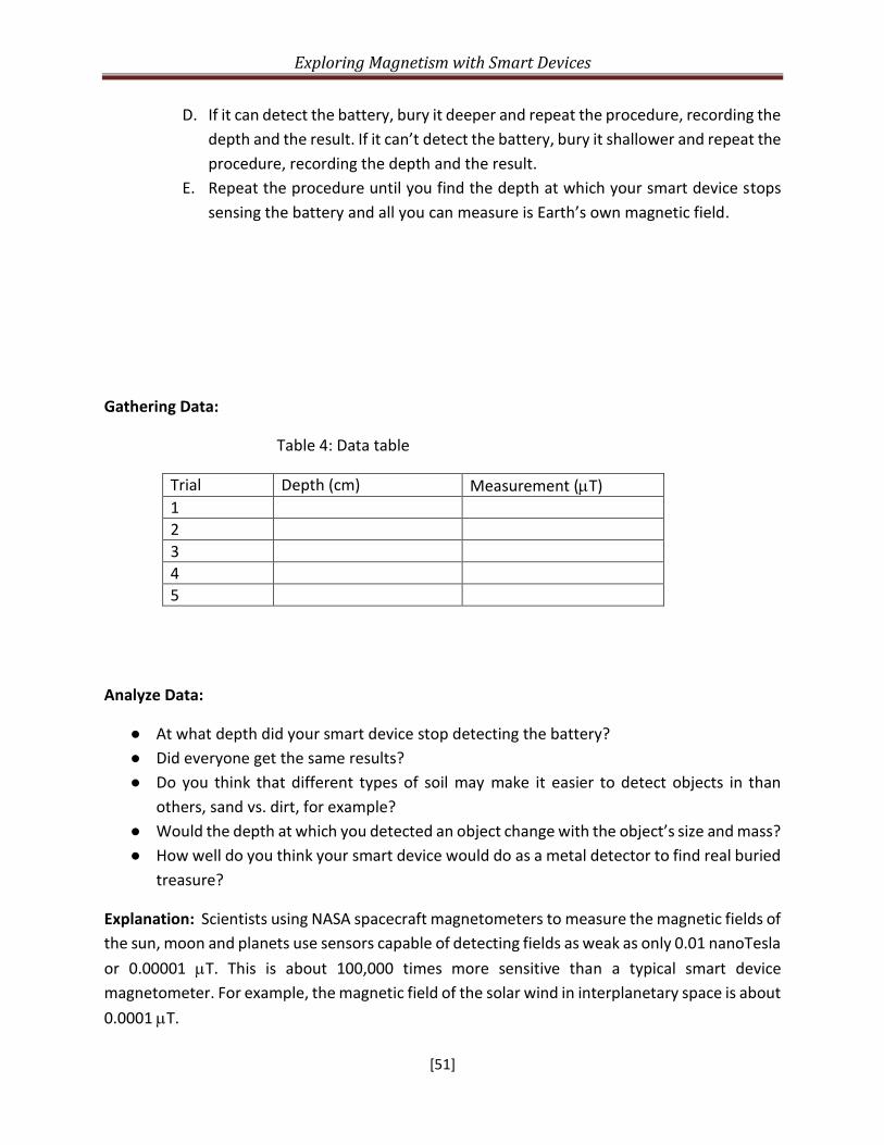
Exploring Magnetism with Smart Devices
[51]
D. If it can detect the battery, bury it deeper and repeat the procedure, recording the
depth and the result. If it can’t detect the battery, bury it shallower and repeat the
procedure, recording the depth and the result.
E. Repeat the procedure until you find the depth at which your smart device stops
sensing the battery and all you can measure is Earth’s own magnetic field.
Gathering Data:
Table 4: Data table
Trial Depth (cm) Measurement (T)
1
2
3
4
5
Analyze Data:
● At what depth did your smart device stop detecting the battery?
● Did everyone get the same results?
● Do you think that different types of soil may make it easier to detect objects in than
others, sand vs. dirt, for example?
● Would the depth at which you detected an object change with the object’s size and mass?
● How well do you think your smart device would do as a metal detector to find real buried
treasure?
Explanation: Scientists using NASA spacecraft magnetometers to measure the magnetic fields of
the sun, moon and planets use sensors capable of detecting fields as weak as only 0.01 nanoTesla
or 0.00001 T. This is about 100,000 times more sensitive than a typical smart device
magnetometer. For example, the magnetic field of the solar wind in interplanetary space is about
0.0001 T.

Exploring Magnetism with Smart Devices
[52]
Assessment: To assess students' understanding of how to use a smart device magnetometer,
look at the data students have gathered to determine if it is accurate. Look at student answers
to the questions in the analysis to assess how students are thinking about the strength and size
of magnetic fields. Try Math Problem 7.
Heliophysics Connection: The Sun and stars are too far away to go digging for treasure, but
astronomers have invented instruments that can allow us to study the magnetic fields of the Sun,
as well as other stars in the universe. Astronomers have been studying the Sun for a long time
and noticed that every 11 years the Sun has more spots on its surface at times, and less spots on
its surface at times. Scientists call these spots ‘sunspots.’ sunspots are spots on the Sun’s surface
that are cooler than the other parts, which can make some wonky things happen with the
magnetic field of the Sun, including the switch of the Northern and Southern Poles of the Sun’s
magnetic field.
Figure 26- Eleven years in the life of the Sun, spanning most of solar cycle 23, as it progressed from solar minimum
(upper left) to maximum conditions and back to minimum (upper right) again, seen as a collage of ten full-disk images
of the lower corona. (Image Credit: NASA)
Exploring Magnetism with Smart Devices
[53]
Middle School Experiments (Grades 6-8) Students at this level most likely have already experienced ‘playing’ with magnets and
have observed how like poles (North to North) repel and opposite poles (North to South) attract.
These experiments are designed to build on those qualitative observations by introducing
students to the basic features of magnetic fields using a smart device magnetometer. Using smart
device tools gives students the opportunity to start to observe magnetic properties quantitively.
At this level, the experiments are designed to guide students through measuring different
components of a magnetic field. Magnetic fields are measured by their amounts along each of
the three directions to space: X, Y and Z, which are defined by the smart device coordinate
system. These values: Bx, By and Bz are reported simultaneously, and are displayed on real-time
graphs. The middle school experiments in this guide require a smart device magnetometer app
that shows the three components of the magnetic field (x, y, z) and provide real-time graphs of
the data. They typically have displays like the ones shown in figure 27.
In addition to a smart device, the experiments at this level require students to explore
magnetism using simple bar magnets, described as ‘toy magnets’ because they are not used in
industrial settings. Strong industrial magnets, cow-magnets for example, can cause injury and
may even cause damage to electronic devices. Additional materials needed for these
experiments include simple compasses, iron nails, batteries, wires, a sample of lodestone
(magnetite) and various other household items to test for magnetic fields. The experiments don’t
have to be done in order, but they are designed to scaffold knowledge and build on skills as the
experiments progress.
As described in Chapter VI there are many of these apps to choose from on both the iOS and
Android platforms. Prior to beginning any experiments, make sure to instruct your students on
which app they should install and guide them through the installation.

Exploring Magnetism with Smart Devices
[54]
Figure 27- Apps with graphical displays from left to right: Physics Toolbox, Sensor Kinetics, Teslameter-11th.
Overview of Middle School Experiments:
M1: Comparing Smart Device Orientation to Compass Bearings: Students at this level are
familiar with a basic compass. In this experiment students will compare the smart device
magnetometer measurements to how a compass works. This is a good opportunity to guide
students through the installation and setup of the magnetometer app.
M2: Measuring the Magnetic Polarity of a Bar Magnet: Students at this level are familiar with
the polarity of a magnet. In this experiment students will use their smart device magnetometers
to identify the north and south poles of an unmarked magnet.
M3: Calculating the Total Magnetic Field: In this experiment students will learn more about how
magnetometers work by using the three dimensions of a magnetic field (X, Y, Z), explored in
Experiment M1, to calculate the total magnetic field of where they are located. The strength of
the total magnetic field varies on Earth depending on location.
M4: Comparing Earth’s Magnetic Field: In Experiment M3 students learned how to calculate the
total magnetic field, B, from the 3 measurements taken by the magnetometer (Bx, By, Bz). In this
experiment students will observe how the magnetic field changes as they adjust the location and
orientation of the smart device.
M5: Comparing Magnetic Compass Apps: This experiment requires an additional smart device
application that uses the magnetometer to display geomagnetic coordinates, also known as a
compass app such as Compass X or GPSCompassBasic. Students will be outside to make
measurements, away from interfering magnetic sources like power lines and motors (air

Exploring Magnetism with Smart Devices
[55]
conditioning systems). Students will use their smart device magnetometer to determine the
accuracy of a compass app for detecting True Magnetic North.
M6: Measuring Your Magnetic Environment: In Experiment M4 students discovered that the
magnetic field doesn’t change significantly in a single location. In this experiment students will
take measurements in a larger area and make a ‘magnetic anomaly map’ of their school
environment, showing how the varying magnetic field of the Earth can be observed in a larger
area. Considering safety factors for your students, determine what area you want your students
to map. This area could be just the school yard or a larger area.
M7: Examining the Magnetic Properties of Lodestone: In Experiment M6 students created a
magnetic anomaly map and learned that deposits of iron and other metals in rocks can cause the
readings to change or cause an anomaly in the Earth’s magnetic field. In this experiment students
will measure the magnetic properties of a sample of lodestone (magnetite), which is found in
many rocks around the world. Large deposits of this mineral can cause noticeable anomalies in
the Earth’s magnetic field.
M8: Measuring the Strength of an Electromagnet: In this experiment students will use their
smart device magnetometer to measure the magnetic field of a simple electromagnet and
observe how the strength of the field changes with distance. At this level students have probably
done experiments with electromagnets before and are familiar with the concept that an electric
current can produce a magnetic field. That is why in some of the previous experiments, students
went outside, away from electrical appliances, to take measurements.
M9: Number of Loops of Wire in an Electromagnet: This experiment is an extension of the
Experiment M8. Instead of measuring how distance affects the strength of the magnetic field,
students measure how the number of coils of wire in the electromagnet affect the strength of
the magnetic field.
M10: Diagraming Electromagnetic Fields with a Smart Device: In the previous experiments,
students measured the strength of an electromagnet and analyzed how distance and number of
loops in the wire affected the strength of the magnetic field. In this experiment students will use
a set of four mini-compasses and a smart device magnetometer to map the direction of the
magnetic field in a wire carrying an electric current. Students will examine the shape of the field
compared to the magnetic field of a simple bar magnet.

Exploring Magnetism with Smart Devices
[56]
❑ Experiment M1- Comparing Smart Device Orientation to Compass
Bearings
Overview: Students at this level are familiar with a basic compass. In this experiment students
will compare the smart device magnetometer measurements to how a compass works. This is a
good opportunity to guide students through the installation and setup of the magnetometer app.
Objectives: Students will be able to apply magnetic field measurements on the smart device
magnetometer (XY coordinates) to the geographic coordinate system (latitude, longitude) used
on maps and with GPS directions (North, South, East, West).
Materials:
● Smart device with a magnetometer app installed
● Compass with a needle
Background: The compass needle aligns with Magnetic North-South and the directions
perpendicular to the needle are Magnetic East-West. A compass needle located in the Northern
Hemisphere of Earth always points to the Magnetic North Pole; in the Southern Hemisphere it
points to the Magnetic South Pole. However, the Magnetic Poles are not exactly in the same
location as the Geographic Poles drawn on maps or globes. This is because Geographic Poles are
fixed locations on the Earth (00 latitude) and the magnetic field of the Earth is constantly
changing. One day the magnetic field of the Earth will flip completely, and the North and South
Poles will reverse their polarity.
Professional magnetometers are lined up so that they measure the magnetic coordinates in the
geophysical coordinate system (X, Y, Z), or latitude X, longitude Y, and elevation Z. Smart devices
also measure coordinates in 3 dimensions but in terms of their Body Frame, shown in figure 29.
When the phone is placed flat on a table top, X is along the short axis of the phone; Y is along the
long axis of the phone; and Z is pointing downward. This is important for navigating with the
smart device so it can locate your position on Earth as you move your device. The relationship
between the X and Y coordinates is used by a compass to get your magnetic bearing.
Geomagnetic X: represents the magnetic field strength in the direction of the north
magnetic pole. For your smart device, this direction will be the phone’s long-axis (By) with
positive values increasing to the north and negative values directed south.
Geomagnetic X = smart device By

Exploring Magnetism with Smart Devices
[57]
Geomagnetic Y: represents the magnetic field strength 90 degrees from the x-direction
in the “magnetic east” direction. For your smart device, this direction is along the short
axis (Bx) with positive values directed eastwards and negative values westwards.
Geomagnetic Y = smart device Bx
Geomagnetic Z: represents the magnetic field strength in the local nadir direction
(vertically down) with positive values towards nadir and negative values towards zenith
(vertically up). For your smart device, the z-axis values (Bz) are reversed and positive
towards zenith and negative towards nadir.
Geomagnetic Z = - smart device Bz
Figure 29- Body Frame coordinates for smart devices showing the axis labels and the direction of positive change. The origin of the coordinate system is at the middle of the phone casing.
Question: How does a smart device magnetometer compare to a compass?
Procedure:
Part A: Orienting your smart device
Step 1) First, place your smart device on a leveled table top. That ensures that your smart device’s
Z axis is parallel to the geophysical Z axis, and that your smart device’s X and Y axis are in the
same horizontal plane as the geophysical X and Y axis.
Step 2) Orient your phone to magnetic north. To do this, rotate your smart device on the table-
top until the Bx value reaches a minimum, which should be near zero. Your smart device is now
aligned with the geomagnetic coordinate system with its y axis pointed to Magnetic North.

Exploring Magnetism with Smart Devices
[58]
Gathering Data:
Step 3) Sketch your classroom and note the location of your desk. Label magnetic north on your
drawing. What direction is your desk facing?
Analyzing Data: Compare the accuracy of your smart device magnetometer to a simple compass.
Place the compass on the table next to your smart device. Does the compass show the same
magnetic north as the smart device magnetometer? Draw and label the compass on your
drawing.
Explanation: Smart devices have their own coordinate systems that change as you move the
smart device around. If you place the smart device on a table, you can rotate the device until its
coordinate system matches the Magnetic coordinate system that is registered by the device’s
magnetic sensors. App designers use this principle to allow their navigation displays to work
properly.
Assessment: Look at students' drawings to determine if they are accurately reading their smart
device magnetometer. The compass will also help students confirm that they are making an
accurate measurement. Try Math Problem 11
Heliophysics Connection: Every scientific instrument provides its own frame of reference called
a coordinate system, which can be defined in many ways. Most often it is defined by features of
the instrument itself shown in figure 30, such as its length (long axis), width (short axis) and height
(vertical axis)- as in the case of the smart device Body Axis. A spacecraft instrument has similar
features. Just like our smart device magnetometers coordinate with Earth’s geomagnetic
coordinate systems to help us navigate with using the Global Positioning System (GPS), for
example, spacecraft magnetometers can coordinate with the geomagnetic coordinate system of
the planet they are orbiting, including the Sun. Studying magnetic fields can help us learn a lot
about different objects in the universe.

Exploring Magnetism with Smart Devices
[59]
Figure 30- The NASA /JPL Far Ultraviolet Spectroscopic Explorer (FUSE) has its own coordinate system defined by
features of the spacecraft body. This coordinate system is used by individual instruments to define their
observations. (Credit: NASA/JPL/FUSE)

Exploring Magnetism with Smart Devices
[60]
❑ Experiment M2- Measuring Magnetic Polarity with your Smart Device
Overview: Students at this level are familiar with the polarity of a magnet. In this experiment
students will use their smart device magnetometers to identify the north and south poles of an
unmarked magnet.
Objectives: Students will be able to use their smart device magnetometer to measure magnetic
polarity.
Materials:
● smart device with a magnetometer app installed
● A toy bar magnet with its poles labeled
● An unmarked magnet (take a marked magnet and tape over the markings)
Background: Magnets and magnetic fields are defined by their intensity in different points in
space, as well as their polarity, commonly referred to as ‘north’ and ‘south.’ Magnets have two
poles, but unless they are marked in some way you cannot tell which end is north and which end
is south. Smart devices can be used to measure magnetic polarity.
Students learned in Experiment E1 that the rectangular case of a smart device will have
its long dimension along the Y-axis and its short dimension along its X-axis (see figures 21 and
30). Hold your smart device in its normal operating position. This will define your device’s
coordinate system so that the Y-axis is pointed towards and away from you, and the X-axis points
from side-to-side.
When you measure a magnetic field, you will usually point your device so that the Y-axis
is towards the object. In this experiment, it will be pointed towards the magnet. The
magnetometer app will be running and making measurements of the magnetic field along the X
and Y axis of your device, which the app display will note as Bx and By. Because you will have the
magnet along the Y-axis, you will look at the ‘By’ measurement displayed by the app.
Question: How can you tell which end of a magnet is north and which one is south, if it isn’t
labeled?
Procedure:
Step 1) Place the marked bar magnet at the edge of a table top.

Exploring Magnetism with Smart Devices
[61]
Gathering Data:
Step 2) With your magnetometer app running, point the top of your smart device at the end of
the marked magnet with the smart device held as close to the plane of the table top as possible.
Note whether the sign of the Y component By is positive or negative.
Step 3) Reverse the marked magnet so that the opposite pole is at the edge of the table. Repeat
Step 2. Note that the South Pole pointed at the smart device along the Y axis shows a positive
value, while the North Pole shows a negative value as shown in figure 31.
Step 4) Replace the marked magnet with the unmarked magnet and repeat the measurement in
Step 2.
Figure 31- A magnetometer app that includes a direction arrow. Most other apps just show the values for Bx, By and Bz. The location of the Hall sensor is shown by the yellow rectangle. For a North-type polarity, the arrow points downwards (negative values of Y and By). The convention is that magnetic field lines have arrows drawn on them that point in the direction of the South polarity.

Exploring Magnetism with Smart Devices
[62]
Analyzing Data:
Step 5) Have someone randomly place the unmarked magnet on the table without you seeing.
Based on your experience with the Y axis (By) reading of the marked magnet, what would you
assign as the polarity of the unmarked magnet?
Explanation: The magnetic field of a toy magnet has a polarity, which means that the magnetic
lines of force have a specific direction in space. At the north pole of a magnet the lines are
directed outwards away from the magnet. When a smart device is placed pointing towards this
pole along the smart device Y-axis, the magnetic line of force will be pointed towards negative
values along the devices Y-axis. At the south pole, the magnetic lines of force are directed
towards the magnet and along the positive direction of the devices Y-axis. This fact allows a smart
device to be used to determine the polarity of a magnet that the device is pointed towards.
Assessment: Have students draw a diagram showing the magnetic polarity of each magnet and
the orientation of the smart device. Have students record the measurements from the
magnetometer and how the values determine the polarity of the magnets. Encourage students
to draw in the magnetic field lines of the magnets. Try Math Problem 13.
Heliophysics Connection: Astronomers have been studying the Sun for a long time and since the
1800’s they have noticed that every 11 years the Sun has more spots on its surface at some times,
and less spots on its surface at other times. Scientists call these ‘sunspots.’ Sunspots are locations
on the Sun’s surface that are cooler than the other parts, which can make some interesting things
happen with the magnetic field of the Sun. These sunspots resemble bar magnets and display
north and south- type polarities caused by the directions of the currents from which they are
created. Astronomers can map out the polarity of sunspots to trace out how spots are connected
to each other.
Figure 32- NASA/SDO HMI imagery showing complex sunspot region AR2673 in visible lights (left) and magnetogram (right). Blue indicates a north-type polarity and red indicates a south-type polarity. (Credit: NASA/SDO)

Exploring Magnetism with Smart Devices
[63]
❑ Experiment M3 – Calculating the Total Magnetic Field
Overview: In this experiment students will learn more about how magnetometers work by using
the three dimensions of a magnetic field (X, Y, Z), explored in Experiment M1, to calculate the
total magnetic field of where they are located. The strength of the total magnetic field varies on
Earth depending on location.
Objective: Students will be able to use the three components of a magnetic field to calculate
the total magnetic field using the Pythagorean Theorem.
Materials:
• Smart device with a magnetometer app installed
• Graph paper marked with centimeter intervals
• Metric ruler marked in millimeters
• Calculator
Background: The smart device display provides a real-time trace of the strength of each of the
three magnetic components (Bx, By, Bz). Sometimes the displays seem to change the same way
but at other times the three values change differently. This is like the shadow of a meter stick on
the floor changing its length as you tilt and rotate the meter stick on one of its ends. Using the
measurements of the three components, you can calculate the total magnetic field B, measured
in microTeslas (T).
Gathering Data:
Step 1) Turn on the smart device and place it flat on a table.
Step 2) Write down the three values for the magnetic field, Bx, By and Bz, from the graph
display or from the digital display on the magnetometer.
Analyzing Data:
Step 3) On your graph paper, draw a standard coordinate grid (x-axis and y-axis).
Step 4) Using a scale of 10 T = 1 centimeter, draw a line AB along the x-axis with B located at
the origin; the length of line AB should match the value of the Bx-value in step 2. Label the x-
axis Bx. See figure 33.
Step 5) Using a scale of 10 T = 1 centimeter, draw a line BC along the y-axis with B located at
the origin; the length of line BC should match the value of By-value in step 2. Label the y-axis
By. See figure 33.

Exploring Magnetism with Smart Devices
[64]
Step 6) Connect Points A and C to form a right triangle. Label the line AC (the hypothenuse of
the triangle) Bh. See figure 33.
Step 7) Use the Pythagorean Theorem to calculate the Bh value.
Figure 33- The geometry of the X-Y plane and direction of Bh (arrow).
Step 8) Draw a second identical coordinate grid with B at the origin and line AB along the x-axis
and line BC along the y-axis.
Step 9) Using the same scale, 10 T = centimeter, draw line AB (x-axis) using the Bh-value in the
right triangle from step 10. Label the x-axis Bh.
Step 10) Using the same scale, 10 T = centimeter, draw line BC (y-axis) using the Bz-value in
step 2. Label the y-axis Bz.
Step 11) Connect points A and C to form a right triangle. Label the line AC (the hypothenuse) B.
Step 12) Use the Pythagorean Theorem to calculate the B value in the second triangle (the total
magnetic field).
Confirm your calculations using a second method:
Step 13) For each component of the magnetic field measured in Step 2 (Bx, By, Bz), calculate
the square of each value to two decimal places.
Step 14) Calculate the sum of the squares of the three components calculated in Step 13.
Step 15) Take the square-root of the sum calculated in Step 14. This is the total strength of the
magnetic field B (units =T). Total Strength of the Magnetic Field: B = ((Bx)2 + (By)2 + (Bz)2)
Explanation: The two methods should give the same value for the total magnetic field (B) because
they both use the values of Bx, By and Bz to form a 3-dimensional triangle in space. This is

Exploring Magnetism with Smart Devices
[65]
equivalent to determining the length of a tilted meter stick by measuring the length of its shadow
along the vertical and horizontal directions.
Assessment: Students should be able to extract magnetic measurements from the graph display
on the magnetometer app and then use two different methods to calculate the total magnetic
strength, B, from the three component values. Try Math Problems 8, 9, 10.
Heliophysics Connection: When spacecraft pass-by or orbit a planet, their magnetometers detect
the three components of the local magnetic field at each point in space. Scientists can convert
these measurements into various maps of the planet’s magnetic field including its shape in space
and its intensity. This provides valuable information into the condition of the planets core. A very
weak field means that the core is likely solid and non-metallic while a strong field usually means
that the core is molten, rich in iron and rapidly spinning.
Figure 34- Mercury has a weak magnetic field that can be detected by the NASA MESSENGER spacecraft. This plot
shows the total intensity, B, of the magnetic field in the vicinity of the planet and reveals the important
components of the planet’s magnetic field. (Credit: NASA/MESSENGER)

Exploring Magnetism with Smart Devices
[66]
❑ Experiment M4- Comparing Earth’s Magnetic Field
Overview: In Experiment M3, students learned how to calculate the total magnetic field (B) from
the three measurements taken by the magnetometer (Bx, By, Bz). In this experiment students
will observe how the magnetic field changes as they adjust the location and orientation of the
smart device.
Objectives: Students will be able to compare the total strength of Earth’s magnetic field as they
adjust the location and orientation of the smart device.
Materials:
● Smart device with a magnetometer app installed
Background: Magnetic field measurements are not like measuring temperature with a
thermometer or mass with a bathroom scale. Magnetism is measured at every point in space by
three quantities called components. Physicists and mathematicians call magnetism a ‘vector’
because it has both magnitude and a direction in space. Because space is 3-dimensional, we need
three numbers that measure how long the vector is along each direction. This is like measuring
the shadow on the ground of a tilted meter stick. The relationship between the length of the
vector, B, called its magnitude, and the component measurements Bx, By and Bz is given by using
the Pythagorean Theorem. In figure 35 the intensity of the magnetic field, H, is computed from
the two components X and Y. For example, if your magnetometer measures X = 3.0 T and Y =
4.0 T, then H = 5 T.
Figure 35- The use of the Pythagorean theorem applied to magnetic field components X, Y and their combined
magnitude H.

Exploring Magnetism with Smart Devices
[67]
Question: How does the total strength of Earth’s magnetic field change as you move the smart
device?
Procedure:
Step 1) Place your smart device on a table top and start the magnetometer app. Make sure it is
as far away from nails in the table, metal fasteners or other environmental sources of metal
within a meter of the smart device. These can throw off the readings because they are
ferromagnetic.
Gathering Data:
Step 2) Note the X, Y and Z values that show up on the plot or in the digital display; for example:
X=20.5 μT, Y=-3.0 μT and Z=-41.3 μT.
Step 3) Use the Pythagorean Theorem H2 = X2 + Y2, shown in figure 35 to find the strength of
Earth’s magnetic field, H, in the plane of the table top. For example, if X=20.5 T and Y=-3.0 T
and Z= -41.3 T then H= +20.7 T and Z=-41.3 T.
Step 4) Use the Pythagorean Theorem again B2= H2+Z2, to measure the total magnetic field
strength. For example, with H=20.7 T and Z=-41.3 T, B = 46.2 T.
Step 5) Rotate the smart device 45 degrees from its previous position and repeat the calculations
outlined in step 3. Calculate H, Z and B.
Analyzing Data: Compare the measurements taken in Step 1 and Step 5. Which magnetic field
values (X, Y, Z, H, B) change and which values remain about the same?
Explanation: You should notice that the B, H and Z values do not change. This is because the
value for B and Z from Earth’s magnetic field do not change very much at a given location,
however the X and Y values will change as you rotate the smart device in the horizontal plane
because it is now acting like a compass to detect Magnetic North. The magnitude of H in the
horizontal plane will not change as you rotate the smart device because this part of earth’s
magnetic field is also constant for a particular location in the field. Although the magnitude of H
does not change, its direction in the X and Y coordinates will change. This is the basis for magnetic
compass apps and how they measure your magnetic bearings on the surface of Earth.
Assessment: Check students’ calculations and data analysis to determine if they used the
magnetometer with accuracy and precision and did the calculations correctly by applying the
Pythagorean Theorem. Try Math Problems 8, 9, 10, 12.

Exploring Magnetism with Smart Devices
[68]
Heliophysics Connection: Earth’s magnetic field has been intensively studied from the ground
for over 400 years but only in the last 60 years have spacecraft been able to measure and explore
its magnetic field in space. The first mission to make this measurement was Explorer 3, which
confirmed the theory that radiation belts trapped by Earth's magnetic field exist around the
planet. Later, NASA's Pioneer 5 launched in March 1960, provided the first map of the
interplanetary magnetic field between Earth and Venus. A schematic drawing and artist
rendering of this field is shown in figure 36. Earth’s magnetic field has a comet-like shape with a
tail that points directly away from the sun. This ‘geomagnetic tail’ is the source of the charged
parti les that flow into Earth’s polar regions and create the Aurora Borealis (North) and Aurora
Australis (South).
Figure 36- Earth’s magnetic field changes from minute to minute as powerful winds of plasma from our sun pass-by,
but its general shape looks like a bar magnet close to Earth’s surface, but with a long tail f magnetism that extends
beyond the orbit of the moon. Millions of measurements by spacecraft have been used by scientists to model the
shape of this field even though it encompasses trillions of cubic kilometers of space. This figure is one rendering of
the field. The yellow dot in the upper right is our Moon. (Credit: NASA/JPL/E. Masongsong).

Exploring Magnetism with Smart Devices
[69]
❑ Experiment M5- Comparing Magnetic Compass Apps
Overview: This experiment requires an additional smart device application that uses the
magnetometer to display geomagnetic coordinates, also known as a compass app. Take students
outside to make measurements, away from interfering magnetic sources like power lines and
motors (air conditioning systems). Students will use their smart device magnetometer to
determine the accuracy of a compass app for detecting True Magnetic North.
Objective: Students will be able to compare the accuracy of a compass app using their smart
device magnetometer.
Materials:
● Smart device with a magnetometer app and a magnetic compass app installed. Examples
can be found by searching the app store for ‘compass’ and include such possibilities as
Compass-X and GPSCompassBasic. The compass app should be switchable between ‘true
bearing’ and ‘magnetic bearing’.
● A standard protractor
● Graph paper
Background: Our Earth has a North Pole and a South Pole, which form an axis about which the
planet rotates once each day. Navigation maps are oriented with these poles to form the latitude
and longitude system for locating cities and other geographic features. Because Earth’s core is
generating a magnetic field, Earth also has a North and South Magnetic Poles, but these are not
lined up exactly with the geographic poles. Navigators have used magnetic compasses to identify
the direction to the North Magnetic Pole called a Magnetic Bearing angle, and then correct this
angle to find the direction to the geographic North Pole called the True Bearing.
Most compass apps use the smart device magnetometer to determine the
direction to Magnetic North, then use the smart device orientation information to determine in
which direction you are pointing so that the Magnetic Bearing can be calculated. By
supplementing this with GPS information, the correction to get the True Bearing can be deduced.
Similar calculations apply in the Southern Hemisphere.
A magnetic compass works by sensing the Bx and By components of Earth’s
magnetic field. The needle points in the direction of H in figure 37, which is always in the direction
of Earth’s magnetic North Pole. If you want to find the Magnetic Bearing that corresponds to
how your street is oriented, you point the magnetic compass so that its X axis is lined up with the
street. The magnetic compass needle will point along the H direction, and the angle between X
and H is the Magnetic Bearing angle.

Exploring Magnetism with Smart Devices
[70]
Figure 37- The geometry of the H magnetic component in the horizontal plane.
Question: How does a compass app calculate the magnetic bearing?
Procedure:
Prepare Materials:
Step 1) Draw a graph with 4 quadrants. Label all 4 axes with 5 μT intervals. The vertical axis is
the value of the By measurement and the horizontal axis is the corresponding Bx measurement.
See figure 38 for an example.
Figure 38- Example of the scaled graph.
Step 2) Download the appropriate compass app and select the ‘magnetic bearing’ feature.

Exploring Magnetism with Smart Devices
[71]
Step 3) Smart devices have to be calibrated periodically so that their magnetometers and
compass apps read correctly. Do this by holding the device and waving it through a Figure-8 path
for a few seconds. This path is shown in figure 17. The apps will use the magnetic measurements
to identify the strength of Earth’s fixed magnetic field strength and use this to calibrate its
magnetism scales.
Step 4) At an outside location far from interfering electrical equipment, place your smart device
on a horizontal surface. This ensures that the device X and Y coordinates are in the horizontal
plane of the Earth at your location. Using the compass app, rotate the smart device until the
compass bearing shows due North (0o or 360o).
Step 5) Select the ‘true bearing’ function and record the value in table 7 column 2. This is the
bearing with respect to Geographic North Pole that is used in a map.
Step 6) Calculate the difference between the true and magnetic bearing and record the value in
the data in table 7 column 3. For example, the magnetic bearing might say 0o while the true
bearing might say 349o for a difference of (0-349 = -11o). This difference is what navigators call
the Declination.
Step 6) Return to the app’s ‘magnetic bearing’ function and confirm that the compass is still
pointed to 0o Magnetic North.
Step 7) Without moving the smart device, carefully close the compass app and open the
magnetometer app. Mark the point on your graph to the corresponding average Bx and By values
measured by the magnetometer app.
Step 8) Draw a vertical line from the point to the horizontal axis. Draw a line from the origin to
the point. You should have drawn a right triangle like the one in figure 37.
Step 9) With a protractor, measure the angle from the X-axis to the hypotenuse, H, of the
triangle. Record this angle in Column 4 of table 7.
Step 10) Have students test another compass app and compare the accuracy of the two.
Gathering Data:
Table 7: Data table
Magnetic Bearing True Bearing Calculated Difference Angle of X-axis
0o or 360o - North
90o or East
180o or South
270o or West
Analyzing Data: Compare the calculated difference between magnetic bearing and the true
bearing with the angle in Column 3, and the angle in Column 4 from your graph. Are they close
in value? Which app that you tested is more accurate?

Exploring Magnetism with Smart Devices
[72]
Explanation: As shown in table 8, most compass apps can determine the direction to Magnetic
North to within about 2o. This is good enough for crude measurements in navigation over short
distances, but for a journey of more than 1 kilometer your 2o direction error will get you more
than 35 meters off course. The compass apps all use the same sensor as the magnetometer.
Table 8: Example of measurements for detecting Magnetic North
App Name Cost Magnetic Bearing to
North (360o)
Difference between Magnetic Bearing and
True Bearing
Compass Free 358o NNW 2o
Compass X Free 352o NNW 8o
GPSCompassBasic $0.99 351o NNW 9o
Average 354 NNW 6o
The accuracy of determining your Magnetic Bearing is limited by the accuracy of the smart device
3-axis magnetometer within the horizontal XY plane. This can vary for smart devices of different
models (iPads, Chromebook, iPhone, Galaxy, etc.). For serious orienteering, it is recommended
that you use high-end compass technology rather than smart devices, because dedicated
magnetic compasses have better magnetic sensitivity.
Assessment: Students can demonstrate knowledge and skills via their data collection, angle
measurements, and data analysis. Have students use ‘claim, evidence, reasoning’ thinking to
communicate their findings. For example, “this compass app is more accurate. The evidence for
this is… which supports my claim because...”. Try Math Problem 8, 9.
Heliophysics Connection: Magnetometers used on spacecraft such as the one shown in figure 39
are highly sensitive instruments that are designed to be compact, light-weight, and consume very
little electrical power. They are designed to precisely measure the intensity, components and
direction of magnetic fields from Earth, the Sun and planets among other magnetic objects. By
measuring very accurately the magnetic fields they encounter, spacecraft can use this
information to orient themselves in space.

Exploring Magnetism with Smart Devices
[73]
Figure 39- The magnetometer used on the Pioneer 10 spacecraft that was used to measure the magnetic field of
Jupiter. Located on the end of a 7-meter boom, the sensor on the right was capable of measuring magnetic fields
as weak as 0.01 nanoTesla or 7 million times weaker than Earth’s own magnetic field. (Credit: NASA/Pioneer).

Exploring Magnetism with Smart Devices
[74]
❑ Experiment M6- Measuring your Magnetic Environment
Overview: In Experiment M4 students discovered that the total magnetic field, B, doesn’t change
significantly in a single location. In this experiment students will take measurements in a larger
area and make a ‘magnetic anomaly map’ of their school environment, showing how the varying
magnetic field of the Earth can be observed in a larger area. Considering safety factors for your
students, determine what area you want your students to map. This area could be just the school
yard or a larger area.
Objective: Students will be able to identify the geophysical components of a magnetic field and
create a magnetic anomaly map of their area.
Materials:
● Smart device with a magnetometer app installed
● Printer and access to the internet to print local maps
Background: Earth’s magnetic field is present everywhere, but in some places, it is stronger than
in others because of sub-surface deposits of iron and other ferromagnetic ores. Some places even
have lodestone deposits. These places are called magnetic anomalies. The way that these are
detected is by passing the magnetometer across the ground and measuring the vertical
component (Z-direction) of the magnetic field at each spot. A large concentration of iron will
cause this ‘Bz’ component to become more positive. A large void, cave or sub-surface liquid
deposit will cause the Bz component to be weaker.
The average value of Bz at any location is the sum of the measurements divided by the
number of measurements. But no measurement is perfect because there can be many sources
of measurement error and interference (electronic noise in the instrument) that cause repeated
measurements to differ. You can measure this variation by computing the standard deviation
which is usually expressed as plus-or-minus (±) some number. For example, if you measure the
average of Bz to be 45.6 T, the uncertainty for a smart device could be ± 0.2 T so that its actual
value could be between 45.4 T and 45.8 T. In order to really trust that a measurement is
significant and not the result of a random error, typically you only trust measurements that are
3-times the measurement error, which for this example is 0.6 T. So, if you see what you think
might be an anomaly, it has to be stronger that 45.6 + 0.6 = 46.2 T or weaker than 45.6 - 0.6 =
45.0 T to be trusted.
Question: What magnetic anomalies exist in my geographic area?

Exploring Magnetism with Smart Devices
[75]
Procedure:
Step 1) Use Google Earth or some other street map display to select an area around your school
that you are able to map. For example, here is a one-square-mile area around the town of
Poolesville, Maryland. Your area may be a little smaller, depending on where your school is
located and how far you can go on school grounds.
Step 2) Print the map. Lay out a regular grid of 9, 16 or 25 points on the street map. For example,
figure 40 shows a 3x3 grid for a portion of the town of Poolesville, Maryland.
Figure 40- A regular grid of measurement locations spaced about 300 feet apart in the town of Poolesville, Maryland.
(Credit Google Earth)

Exploring Magnetism with Smart Devices
[76]
Gathering Data:
Step 3) Visit each of the locations on the map grid. Use your magnetometer to make a
measurement of the Z component (Bz) of the local magnetic field. Make sure the phone is flat on
a level ground so that the X and Y smart device axis are parallel to the ground in the local
horizontal plane. Bring your map grid, a notebook and something to write with to record values
while in the field. Record the Bz values at each location.
Step 4) After returning to your classroom, plot these measurements on each of the corresponding
points on the map. Here is an example of what such a plot might look like in Figure 41 for a simple
3x3 grid.
Figure 41- An example of a grid of Bz measurements
Analyzing Data:
Step 5) Find the average value of all of the measurements. This value represents the average
value of Earth’s magnetic field over this region. In this example, the average of the nine
measured values in figure 37 is <Bz> = (47.3 + 46.4 +47.2 + 47.5 + 48.5 + 47.2 + 47.1 + 46.9 +
47.3)/9 = 47.267 T but because we only have three significant figures, we round this calculated
number to 47.3 T.
Step 6) Subtract the average value from all of the grid measurements. The result is a measure of
how the local field fluctuates from the geomagnetic field, or magnetic anomalies. This could be
due to underground deposits of minerals, large metal pipes, and other objects.

Exploring Magnetism with Smart Devices
[77]
Top Row: 0.0 -0.9 -0.1 Middle Row: +0.2 +1.2 -0.1 Bottom Row: -0.2 -0.4 0.0
Step 7) Find all locations where this difference is greater than the statistical uncertainty in the
measurement, which is about 0.15 μT. Locations that have deviations of 0.5 μT or larger have
significant subsurface interference. From the example in Step 6, there are two points that meet
this requirement: Top Row center value of -0.9 T and Middle Row center value of +1.2 T.
Figure 42- Magnetic anomaly map for Illinois, Indiana and Ohio. Note that the anomalies can be both positive
(purple) and negative (blue). (Credit: USGS/https://pubs.usgs.gov/ds/321/ilinoh.htm)
Explanation: Figure 42 is a map of Illinois, Indiana and Ohio showing magnetic variations. Called
a magnetic anomaly map, the largest deviations (purple) are about +0.35 μT. Earth’s magnetic
field has an average value at the surface that can be mathematically modeled very accurately.
When this model is subtracted from the data, regions where the magnetic field is slightly stronger
or weaker can be mapped. These irregularities often follow deposits of iron (high values) or places
that have lots of non-magnetic materials below the surface such as caves, sinkholes or sandstone
(low values). Geologists also use anomaly maps to identify places with subsurface oil or gas
deposits.

Exploring Magnetism with Smart Devices
[78]
Assessment: Have students create a magnetic anomaly map from their data using color like the
example map above. Ask students to make a hypothesis about what could cause these magnetic
anomalies in their area based on the geographic features near the anomalies they found. Use
student maps to assess the accuracy with which students measured the magnetic field using their
smart devices and check calculations for accuracy. Try Math Problem 1.
Heliophysics Connection: Earth’s magnetic field can be disturbed by magnetic activity on the
Sun. High magnetic activity on the Sun causes storms in space that can affect the magnetic field
of the Earth and can interfere with technology and communication. We call this space weather.
Space weather and solar storms are monitored by NASA scientists and they can detect these
storms by comparing Earth’s magnetic field on the ground during times when no storm is
occurring with times when significant changes are occurring. These storms can be most
commonly viewed on Earth at the poles via the aurora. The Aurora Borealis shown in figure 43
from the International Space Station occurs when the magnetic field is highly disturbed in the
comet-like tail behind Earth. This causes charged particles to flow into the polar regions where
these particles collide with atoms of oxygen and nitrogen to create beautiful displays in the sky.
Figure 43- Aurora seen from the International Space Station. (Credit: NASA/ISS)
Join the CrowdMag citizen scientist community project to help scientists make a detailed map
of Earth’s magnetic field. Citizen scientists are volunteers with an interest in contributing to
actual scientific research projects. For many projects, scientists are in need of data from a variety
of locations around the world and are unable to do the traveling themselves. CrowdMag is a

Exploring Magnetism with Smart Devices
[79]
project by scientists at the National Oceanic and Atmospheric Administration (NOAA) to map
Earth’s magnetic field at ground level at resolutions of 10 km or less. Millions of data
measurements have been made using a free NOAA app called CrowdMag.
Figure 44- An example of measurements made by thousands of amateur scientists across the continental United
States. (Credit: NOAA/CrowdMag).
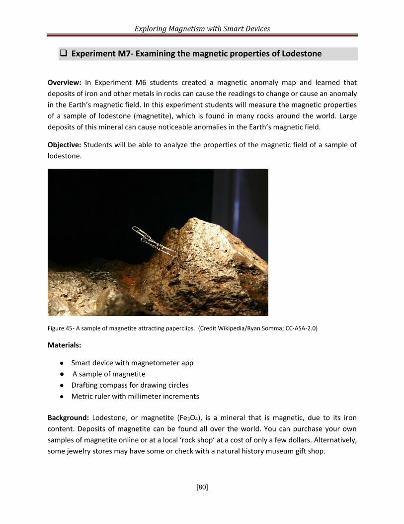
Exploring Magnetism with Smart Devices
[80]
❑ Experiment M7- Examining the magnetic properties of Lodestone
Overview: In Experiment M6 students created a magnetic anomaly map and learned that
deposits of iron and other metals in rocks can cause the readings to change or cause an anomaly
in the Earth’s magnetic field. In this experiment students will measure the magnetic properties
of a sample of lodestone (magnetite), which is found in many rocks around the world. Large
deposits of this mineral can cause noticeable anomalies in the Earth’s magnetic field.
Objective: Students will be able to analyze the properties of the magnetic field of a sample of
lodestone.
Figure 45- A sample of magnetite attracting paperclips. (Credit Wikipedia/Ryan Somma; CC-ASA-2.0)
Materials:
● Smart device with magnetometer app
● A sample of magnetite
● Drafting compass for drawing circles
● Metric ruler with millimeter increments
Background: Lodestone, or magnetite (Fe3O4), is a mineral that is magnetic, due to its iron
content. Deposits of magnetite can be found all over the world. You can purchase your own
samples of magnetite online or at a local ‘rock shop’ at a cost of only a few dollars. Alternatively,
some jewelry stores may have some or check with a natural history museum gift shop.

Exploring Magnetism with Smart Devices
[81]
In this experiment, you will be measuring the magnetic field of a sample of lodestone, but
this sample will be inside the stronger magnetic field of Earth, which is everywhere. Where ever
the lodestone sample is, its magnetic field will be added to Earth’s magnetic field at that location.
To figure out what the lodestone’s magnetic field looks like, when we take each measurement,
we have to subtract the ‘ambient’ magnetic field of Earth’s to get the strength of the lodestone
field at that point.
Question: Does a piece of loadstone have a magnetic field like a typical bar magnet?
Procedure:
Step 1) Start up your smart device magnetometer app and scan it near the sample of lodestone
to see if it registers a magnetic field.
Step 2) Place the lodestone sample on a piece of paper and trace your sample as shown in Figure
44.
Step 3) Use the drafting compass and the ruler to measure and draw a circle on a piece of paper
around your sample- about 20mm greater than the maximum radius of the sample.
Example: A sample has its longest dimension of 48 mm so its maximum radius when centered on
the circle will be (48/2=) 24 mm and the radius of the circle will be (24+20=) 47 mm. The added
distance allows for the difference between the smart device case and the location of the sensor.
Figure 46- An example of the measurement set up. The circle should be big enough that the Hall Effect censor will lay on top of the circumference at each measurement location. Make sure the Y axis of the smart device is pointed towards the center of the circle.

Exploring Magnetism with Smart Devices
[82]
Step 4) Along the circumference of the circle, select at least four equidistant locations and label
them alphabetically (A, B, C, D).
Step 5) Place your magnetometer flat on the table with its front edge touching the circle at point
A, with its Y-axis pointed at the center of the sample circle. Record the measured X, Y, Z values
in the data table columns 1,2 and 3 below.
Step 6) Without moving the smart device, remove the lodestone and make a measurement of
Earth’s ambient magnetic field and enter these numbers in the columns4, 5 and 6 for ‘Ambient
Measurement’. Record the measured X, Y, Z values in the data table below.
Step 7) Carefully replace the lodestone in the exact orientation it was in at the start and repeat
steps 5 - 6 until you have completed all 4 measurements from the points you marked on the circle
around the lodestone (A, B, C, D).
Gathering Data:
Table 5: Data table
Point (1) (2) (3) (4) (5) (6) (7) (8) (9)
X Y Z X Y Z X Y Z
A
B
C
D
Analyzing Data:
● Calculate the magnetic field at each point. To get this value subtract the Ambient (A)
measurements in columns 4, 5 and 6 from the Sample (S) measurements in columns 1,2
and 3 to get the Magnetic Field Values and enter your answer in columns 7, 8 and 9. The
corrected value is the magnetic field of the sample.
● Highlight all the values in your table that have an absolute value greater than |0.5| μT.
That means the value is greater in absolute value than -0.5 or +0.5 (see example below).
If any measurement is stronger than |0.5| μT the magnetite field has been detected.
● How many North and South poles does your sample have? Remember from the last
experiment that a negative y-value indicates the field strength of a north pole and a
positive y-value indicates the field strength of a south polarity. Label these poles on your
drawing. You may only detect one magnetic pole, or several poles of the same polarity if
the opposite pole is not in the plane of the table.

Exploring Magnetism with Smart Devices
[83]
Table 6: An example of the data analysis for two positions 180o apart:
Point (1) (2) (3) (4) (5) (6) (7) (8) (9)
X Y Z X Y Z X Y Z
A 3.5 -15.7 -70.2 4.0 -15.0 -70.5 -0.5 -0.7 0.3
B -14.5 25.7 43.2 -14.0 25.5 -43.5 -0.5 0.2 0.3
Point A shows a magnetic field in the Y direction, as indicated by an absolute value greater than
0.5 μT.
Explanation: Students discover that naturally-occurring magnetic fields can be very complicated
and may not have the paired North-South polarity of a simple bar magnet. In the example above,
we only detect one pole of the sample with a value of -0.7 T because the other pole/poles are
weaker that our 0.5 T limit for detection. If we were to tilt the sample within the circle so that
another plane of the sample is being mapped, we might find a different collection of poles.
Assessment: Examine student drawings, data tables, and calculations to determine if they are
able to correctly analyze the properties of a magnetic field of a sample. Try Math Problem 14.
Heliophysics Connection: The image in figure 47 shows an image of the Sun taken with
instruments on the Solar Dynamics Observatory (SDO). NASA uses data from the SDO mission to
create a map of the Sun’s magnetic field, as seen by the white lines added to the image. These
maps define where intense plasma currents are occurring and from these magnetic fields can be
mathematically calculated.

Exploring Magnetism with Smart Devices
[84]
Figure 47- Mathematical models of the sun’s magnetic field can be created from maps of the x-ray emission from its
surface regions. These maps define where intense plasma currents are occurring and from these magnetic fields can
be mathematically calculated. (Credit: NASA/SDO)

Exploring Magnetism with Smart Devices
[85]
❑ Experiment M8- Measuring the Strength of an Electromagnet
Overview: In this experiment students will use their smart device magnetometer to measure the
magnetic field of a simple electromagnet and observe how the strength of the field changes with
distance. At this level students have probably done experiments with electromagnets and are
familiar with the concept that an electrical current can produce a magnetic field. That is why in
some of the previous experiments, students went outside, away from electrical appliances, to
take measurements.
Objective: Students will be able to analyze data about the strength of a magnetic field collected
using their smart device magnetometer.
Materials:
● A smart device with a magnetometer app
● A common nail
● About one foot (30 cm) of 24-gauge wire
● A D-cell battery
● Tape
● Ruler (cm intervals)
● A paperclip
Background: A simple electromagnet can be created by wrapping wire around a nail and
attaching the ends of the wire to a battery. In 1820, Danish scientist Hans Christian Ørsted
discovered by accident that an electric current flowing through a wire would cause the needle of
a compass to move. Ørsted correctly theorized that electricity created a magnetic field, an
observation that was built upon by other scientists who endeavored to use electricity to create
magnets.
Question: How does the strength of the magnetic field change with distance?
Procedure:
Step 1) Make a simple electromagnet by wrapping a length of wire around a nail and attaching it
to a small battery. Test to see if it is working by trying to pick up a paperclip with the nail. See
figure 49.
Step 2) Place your electromagnet on top of a piece of paper on a flat tabletop. Tape the paper to
the table so that it does not move.

Exploring Magnetism with Smart Devices
[86]
Step 3) On the piece of paper, use a ruler to measure 1 cm increments out from the nail. Mark
them on the paper.
Step 4) With the magnetometer app running, place your smart device at the 1 cm mark, with the
long axis (Y) of the phone pointed at the center of the coil of wire, as shown in figure 48. In figure
49, the current is flowing counterclockwise downwards, from the positive terminal of the battery
to the negative terminal of the battery. Label the direction of the current on the piece of paper.
Figure 48- How to measure the magnetic field of a simple electromagnet. The base of the arrow is where the magnetometer sensor is located on the smart device. The arrow shows the distance to the midpoint of the coil of wire.
Figure 49- An example of a simple electromagnet holding up a paper clip. The positive end of the battery is at the top so the current is flowing down the wire counter-clockwise to the negative battery terminal on the flat end of battery case.

Exploring Magnetism with Smart Devices
[87]
Step 5) Record the values for X, Y and Z in the data table below under X(on), Y(on) and Z(on).
Step 6) Repeat Step 5 but this time turn off the electromagnet so only Earth’s magnetic field is
present. Record the values for X, Y and Z in the data table below under X(off), Y(off), Z(off).
Step 7) Subtract the ‘off’ values from the ‘on’ values at each distance to determine the strength
of the magnetic field around the electromagnet. Record this calculation in the data table below.
Step 8) Repeat steps 5-7 at 2 cm, 3 cm, etc. Complete the data table below.
Gathering Data:
Table 9 Data table with all measurement units in T.
L(cm) X(on) Y(on) Z(on) X(off) Y(off) Z(off) X Y Z
1 cm
2 cm
3 cm
4cm
5 cm
6 cm
Analyzing Data:
● Calculate the magnetic field properties at each distance by subtracting the (off) values
from the (on) values and entering these differences in columns 8, 9 and 10 of Table 9.
● How does the strength of the magnetic field change with distance?
Explanation: It decreases in intensity very rapidly and can’t be easily measured beyond a few
hundred centimeters. Like the gravitational field of Earth, magnetic fields diminish in strength
very rapidly as you get farther away from them. One big difference, however, is that gravity
follows what is called the inverse-square law; as you double the distance, D, the intensity
decreases by a factor of D2. Magnetic fields are more complex but their intensity decreases even
faster and follow an inverse-cube law proportional to 1/D3.
Assessment: Look at student calculations in the data table and their analysis of the data. Have
students use ‘claim, evidence, reasoning’ thinking to communicate their findings. For example,
“the intensity of the field decreases as you increase the distance between the magnetometer and
the electromagnet. The evidence for this is… which supports my claim because...” Try Math
Problem 15.

Exploring Magnetism with Smart Devices
[88]
Heliophysics Connection: Launched in 2018, NASA’s mission Parker Solar Probe is the closest
human-made spacecraft to graze the surface of the Sun, making its closest approach in 2025.
Because we can’t go too close to the Sun to collect data, astronomers learn most of what they
know about the Sun, as well as other far away objects in the universe, from gathering light. Atoms
emit light at specific wavelengths on the electromagnetic spectrum, which serve as fingerprints
for astronomers to examine when they are looking at the composition of faraway objects. When
a strong magnetic field is present, atoms emit their fingerprint lines at pairs of wavelengths,
which make the lines split in two. With sensitive telescopes, scientists can use this atomic light
to map the magnetic intensity in sunspots and other solar features.
Figure 50- The light emitted by atoms in a magnetic field is split into pairs, which can be used to measure the strength of the magnetic field; a process called the Zeeman effect. (Credit: George Hale, The Astrophysical Journal, 1919)

Exploring Magnetism with Smart Devices
[89]
❑ Experiment M9- Number of loops of wire versus magnetic strength
Overview: This experiment is an extension of Experiment M9. Instead of measuring how distance
affects the strength of the magnetic field, students measure how the number of coils of wire in
the electromagnet affect the strength of the magnetic field. Use the same setup as in Experiment
M8.
Objective: Students will be able to analyze data about the strength of a magnetic field collected
using their smart device magnetometer.
Materials:
● A smart device with a magnetometer app
● A common nail
● About 10-feet of 24-gauge wire
● A D-cell battery
● A paperclip
● 2-inch packing tape
Background: A simple electromagnet can be created by wrapping wire around a nail and
attaching the ends of the wire to a battery. The strength of the electromagnet depends on the
intensity of the current supplied by the battery and the number of loops of wire around the nail.
Question: How do the number of loops of wire in an electromagnet affect the strength of the
electromagnet's magnetic field?
Procedure:
Step 1) Place the smart device at one of the distances, L, from Experiment M8.
Step 2) With the same nail, wrap N loops of wire in one tight row across the nail like the example
in figure 51. There will be excess wire but do not cut this wire. It will be used to add more rows
of loops. Leave space on the nail to add additional loops.
Step 3) Cover the row of loops with a piece of tape to keep the rows of loops together. Count the
number of loops and record them in the data table below.

Exploring Magnetism with Smart Devices
[90]
Figure 51- The number of loops of wire determine the strength of an electromagnet. The direction of current flow (positive to negative) also determines the polarity. (Credit Wikipedia)
Step 4) Turn on the electromagnet and measure the On and Off field values, as you did in
Experiment M8.
Step 5) Add a second row of tight loops on top of the other coils and repeat Steps 2, 3 and 4.
Step 6) Repeat Step 5 for several more rows of loops.
Gathering Data:
Table 10: Data table for measurements with all values in T units.
(N) X(on) Y(on) Z(on) X(off) Y(off) Z(off) X Y Z
Analyzing Data:
● Calculate the magnetic field properties at each distance by subtracting the (off) values
from the (on) values and entering the differences in table 10 columns 8, 9 and 10.
● Calculate the total magnetic field strength B using the Pythagorean Theorem in the
equation below. For example, if you measure Bx = 3.0T, By=5.0 T and Bz=4.0 T then B
= 7.1 T. Enter the value in column 11.
𝐵 = √𝐵𝑥2 + 𝐵𝑦2 + 𝐵𝑧2

Exploring Magnetism with Smart Devices
[91]
● From the data in columns 1 and 10, create a graph with the horizontal axis indicating the
number of loops and the vertical axis the value for B. Plot the strength B versus the
number of loops N on a graph. For example, if 2 rows of 10 loops (N=20 loops) produces
B = 2.5 T and 4 rose of 10 loops (N=40) loops produces 5.5 T, plot the points (20, 2.5
T) and (40, 5.5 T).
Explanation: Each loop forms a complete circle of wire that has a surface area, and through this
surface area the current will produce a fixed amount of magnetic ‘flux’. By adding more circles
(more loops of wire around the nail) you increase the magnetic flux through the iron in the nail
and so amplify the magnetization of the nail.
Assessment: Look at student calculations in the data table and their analysis of the data,
including the graph. Have students use ‘claim, evidence, reasoning’ thinking to communicate
their findings. For example, “the intensity of the field increases as you increase the number of
loops of wire on the electromagnet. The evidence for this is… which supports my claim because...”
Try Math Problem 16.
Heliophysics Connection: In this experiment students discovered that the more loops of wire you
add to the electromagnet, the more intense the magnetic field becomes. We have already
discussed that the magnetism we see on the surface of the Sun is produced by plasma, a
superheated state of matter. We also know that there are areas on the surface of the Sun that
are cooler than other places, known as sunspots. sunspots are up to 2,000oC cooler than the rest
of the solar surface (5,500oC). The difference in plasma flow in sunspots, compared to other areas
of the solar surface can increase the strength of the magnetic field they produce until it is strong
enough to pop through the sun’s surface, emerging as two regions of opposite magnetic polarity.
In figure 52, you can observe an actual loop of magnetic lines connecting sunspots, imaged by
the NASA TRACE mission.

Exploring Magnetism with Smart Devices
[92]
Figure 52- This beautiful loop of magnetic lines of force was imaged by the NASA TRACE spacecraft. The field of
view is about 30 times the diameter of Earth across. The origin of the loop is in two sunspots at the base of each
loop. (Credit: NASA/TRACE/M. Aschwanden).

Exploring Magnetism with Smart Devices
[93]
❑ Experiment M10- Diagraming Electromagnetic Fields with a Smart Device
Overview: In the previous experiments, students measured the strength of an electromagnet
and analyzed how distance and number of loops in the wire affected the strength of the magnetic
field. In this experiment students will use a set of four mini-compasses and a smart device
magnetometer to map the direction of the magnetic field in a wire carrying an electric current.
Students will examine the shape of the field compared to the magnetic field of a simple bar
magnet.
Objectives: Students will be able to compare the shape of the magnetic field of a simple bar
magnet and the shape of a magnetic field surrounding a wire carrying an electrical current, using
a smart device magnetometer.
Materials
➢ Smart device with a magnetometer app installed that shows the X, Y and Z components
such as Physics Toolbox.
➢ Mini-compasses (set of 4 for each setup)
➢ A 6x12 piece of white foam board
➢ A screwdriver
➢ 5-feet of 24-gauge insulated wire
➢ A D-cell battery
➢ 2 or three heavy books
Background: When students examine the shape of a magnetic field surrounding a simple toy
magnet, using iron filings for example, they observe that the magnetic field lines form a circular-
type ring flowing from the north and south poles of the magnet. But a straight wire with an
electrical current flowing through it produces a ring-shaped magnetic field around the wire with
no obvious north and south polarity. However, if you bent the straight wire around into a circle,
the resulting magnetic field will have a definite polarity depending on whether the current is
flowing clockwise or counter-clockwise.
Procedure: Note: Teachers will need to prep the materials prior to doing the experiment with
students: Steps 1-6, see figure 53.
Teacher Prep:
Step 1) Use the screwdriver to punch a hole in the foam board about 6-inches from the short
edge of the foam board rectangle
Step 2) Remove insulation from about 1-cm of each end of the wire

Exploring Magnetism with Smart Devices
[94]
Step 3) Thread the wire through the hole 3 or 4 times making a det of 3 or 4 loops of wire. Bend
the wire so that it leaves the hole perpendicular. Secure the wire ring at the edge of the foam
board with a piece of tape so that it remains perpendicular as the wires leave the exit hole.
Step 4) Place the foam board on a table top so that the coil hangs freely as shown schematically
in figure 53. Place the books on the other end so that the foam board is secure.
Figure 53 – A sketch of the coil of wire perpendicular to the surface of the foam board.
Step 5) Before connecting the wire to the battery, place a circle of four compasses around the
wire aligned so that the North markings are all parallel and pointed in the same direction, as
shown in the left image of figure 54. Make sure that the compasses are more than 2-cm from
each other, to prevent the compasses from being attracted to one another. Check this by making
sure all of the needles (the red end in figure 54) are pointed in the same direction (magnetic
north) when no current is flowing in the wire.
Step 6) Check for quality control on the compasses by eliminating those that are not pointing
towards magnetic north. Replace the defective ones with new ones as needed.
Gathering Data Using Mini-Compasses:
Step 7) Have students draw a diagram of the experiment setup on a piece of paper or in their
science journal. Make sure that students label each part of the setup.
Step 8) Attach one end of the wire to the positive terminal of the battery (the end with the
dimple) and the other end of the wire to the negative terminal of the battery (the flat end). Have
students add the battery to their diagram of the experiment, labeling which wire is attached to
the positive terminal and which wire is attached to the negative terminal.

Exploring Magnetism with Smart Devices
[95]
Step 9) Arrange the battery connections so that the current is flowing clockwise away from the
foam board at the exit hole. Current will be flowing from the positive terminal to the negative
terminal. Have students show the flow of current on their diagram using arrows.
Step 10) Once the battery is connected students will observe that the compass needles begin to
move. Once the compass needles stop moving, have students draw the direction of the North
markings (red end in figure 54) of each needle on their diagram, using a different color to show
the new position of the compass needles.
Step 11) Have students draw a circle connecting all the needles and use arrows to indicate which
direction the current is flowing, see the right image of figure 54. Ask students if the current is
flowing clockwise or counter clockwise.
Make a prediction: Ask students what would happen if they switched the wires on the terminal
battery. Would the current flow in the same direction?
*Note: According to the Right-Hand Rule, if your thumb is pointing in the direction of the current,
your fingers will be pointing in the direction of the north magnetic field. You should observe that
if the current is flowing clockwise around the loop of wire, the compass needles will point counter
clockwise.
Caution: Do not leave the wires connected to the battery for a prolonged period of time. The battery will warm up and discharge. Measurements should only take a few seconds so no appreciable heating should occur.
Figure 54- The set up with mini-compasses and arrows showing the direction of the current upwards from the surface. Left) No current flowing so the compasses point towards Magnetic North (Arrow). Right) Current is flowing out (upwards) the foam board (black arrow) and the compasses point in a counter-clockwise direction (red circle)
Gathering Data Using a Smart Device:

Exploring Magnetism with Smart Devices
[96]
Step 1) We will use the Physics Toolbox app for this experiment. Make sure this app is
downloaded and ready to go prior to the experiment.
Step 2) Remove the compasses from the foam board.
Step 3) Place your smart device magnetometer so that the long axis of the smart device points
perpendicular to the foamboard’s longest side. Place the smart device about 8-cm to the left of
the exit hole of the loops of wire.
Step 4) With the current not flowing (battery disconnected), note the direction of Magnetic
North. Take a measurement of the X, Y and Z magnetic components. Have students record these
measurements on a piece of paper or in their science journals.
Step 5) Turn on the current (connect the battery) and note the change in the X, Y and Z
magnetometer values. Have students record these measurements on a piece of paper or in their
science journals.
Analyzing Data:
Step 6) Use the Pythagorean Theorem to calculate the magnitude of the XY field with the current
off and with the current on. Example, OFF) Bx= 30 T By=15 T. ON) Bx=24 T, By = 12 T. so
OFF) |Bxy| = (Bx2+By2)1/2 = 33.5 T. ON) |Bxy| = 26.8 T.
*Note: With the smart device on the foam board, you are measuring the magnetic field of the
wire within the XY plane of the tabletop so these magnetometer values will change the most.
Step 7) Take the difference between the ON and OFF values. Example: 26.8 – 33.5 = -6.7 T. This
is how much the wire’s magnetic field has reduced Earth’s magnetic field in the XY-plane.
Step 8) Take the difference between the ON and OFF values for the Bx and By components.
Example, Bx = 24 – 30 = -6 T and By = 12 – 15 = -3 T. This says that the wire’s magnetic field in
the XY-plane is mostly pointed downwards, which is in the counter-clockwise sense when the
smart device is placed to the left of the wire. The magnitude of the wire’s field at the smart device
is about |Bxy| = 6.7 T.
Make a prediction: Ask students what would happen if they placed the smart device to the right
of the wire. What direction would the magnetic field point?
Explanation: The smart device magnetometer is located in the upper left corner of the case so
this is the location where the magnetic fields are being measured not at the center of the phone.

Exploring Magnetism with Smart Devices
[97]
Also, because the wire’s field is so weak, many smart device magnetic compass apps will not be
able to register the difference between the ON and OFF states.
Assessment: Use student diagrams and predictions to assess their understanding of how the
electric current is affecting the magnetic field of the wire. Check calculations to assess math
skills.
Heliophysics Connection: The sun is a dense ball of plasma heated to 15 milliono C in its interior
and over 5,000oC at its surface. Plasmas are electrically charged and are affected by magnetic
fields. The plasma at the sun’s surface acts like iron filings around a toy magnet or like the
compass needles around the wire. Figure 55 shows how the Sun’s plasma traces out the magnetic
fields above the sun’s surface.
Figure 55- This image taken by the NASA Solar Dynamics Observatory (SDO) on July 12, 2012 shows the x-ray light
produced by plasma at a temperature of over 100,000oF. The plasma traces out the magnetic lines of force that
thread the solar surface revealing many complex shapes. (Credit: NASA/SDO).

Exploring Magnetism with Smart Devices
[98]
High School Experiments (Grades 9-12)
Students at this level are most likely in a higher-level physics course and have taken other
high level science classes. Students should have a solid background in using technology,
specifically spreadsheet software, like Microsoft Excel. MS Excel is a good choice because it is
compatible with most of the magnetometer apps and easily allows students to export data.
These experiments are designed to build on the skills students learned in the experiments
in the Middle School section of the guide in the previous pages. Grade 9 students may benefit
from doing some of the middle school experiments in the previous pages before exploring the
more advanced experiments in this section.
At this level, the experiments are designed to guide students through measuring different
components of a magnetic field. Magnetic fields are measured by their amounts along each of
the three directions to space: X, Y and Z, which are defined by the smart device coordinate
system. These values: Bx, By and Bz are reported simultaneously, and are displayed on real-time
graphs.
High school experiments require a magnetometer app that shows the three components
of the magnetic field (x, y, z) and records and saves the data into a .csv file. Students need an
email address and a laptop with MS Excel installed to analyze data. Other apps may be required
for some experiments. If this is the first time that students are using a smart device to take
measurements using a magnetometer app, consider starting out with Experiment M1. This
experiment will help students become familiar with how the smart device magnetometer relates
to the Cartesian coordinate system used on maps and with GPS directions (North, South, East,
West).
In addition to a smart device, the experiments at this level require students to explore
magnetism using simple bar magnets, described as ‘toy magnets’ because they are not used in
industrial settings. Strong industrial magnets, cow-magnets for example, can cause injury and
may even cause damage to electronic devices. Additional materials needed for these
experiments include simple compasses, batteries, wires, volt meters, resistors, and various
common household items, including some basic tools like a drill. The experiments don’t have to
be done in order, but they are designed to scaffold knowledge and build on skills as the
experiments progress.
As described in Chapter VI there are many of these apps to choose from on both the iOS
and Android platforms. Prior to beginning any experiments, make sure to instruct your students
on which app they should install and guide them through the installation.

Exploring Magnetism with Smart Devices
[99]
Smart Device Recommended App Settings:
● Toolbox - Teslameter 11th (Android; iOS) – Open the Toolbox app. Select the Teslameter
function and press ‘OK’. Tap the parallel line icon on the lower right to start recording
data on the screen. Tap the right arrow to stop recording on the screen Tap the triangle
icon on the top menu bar to open the mail pop-up. Select ‘Mail’. Enter your email address
on the ‘To’ line to send an image of the screen. To send a ‘csv’ file, you need the ‘Pro’
version.
● Tesla Recorder (Android; iOS) – Open the app and tap the first upper-left icon to start the
scan. Tap the second icon to open the recording time menu. Select ‘1 hour’ and tap
‘Done’. Tap ‘Start’ to start recording for up to one hour. Tap the first icon to stop the
recording. On the lower menu bar. Tap the last icon on the right which is the ‘save’ icon.
A menu should open up that shows all the files you have saved. The top file marked with
the date and time is the most recent. Tap the ‘mail’ icon under this file. A pop-up menu
appears and tap the ‘Mail’ icon. Enter your email address in the ‘To’ field and tap the ‘up’
arrow to send it.
● Sensor Kinetics (Android; iOS) – Open the app and select the ‘Magnetometer Sensor’ to
display the graphs. Tap ‘Start’ to begin taking data. Tap ‘Stop’ to stop taking data. Tap the
down arrow on the upper right to open a pop-up menu. Select ‘Files & Sharing’ to open
the list of saved data files. The most recent one is at the top. Tap the file name to open a
pop-up menu. Select ‘Share via E-mail’. Select the ‘CSV Format’ format on the next pop-
up menu. Enter your email address in the ‘To’ line and tap the ‘up’ arrow to send the fila.
● Physics Toolbox (Android, iOS) – Open the app and select ‘Magnetometer’ from the
menu. Tap the + sign to start recording data. Tap the ‘square’ to stop recording. Make
sure in the settings that the graph is turned on under ‘data display’. Fill-in the ‘To’ with
your email address, and ‘Subject’ fields. Tap the up arrow at the top right to send the mail.
From the pop-up menu, tap the ‘mail’ icon.

Exploring Magnetism with Smart Devices
[100]
Overview of High School Experiments:
H1: Using Your Smart Device to Measure Magnetism: This experiment is designed to orient
students to the settings and features of the magnetometer app. Students will practice taking
measurements, exporting the data to a spreadsheet, and analyzing the data by making a graph
using the spreadsheet software.
H2: The Magnetic Field Around a Wire Carrying a Current: In this experiment students create a
typical electromagnet with a nail, wire, and battery and use their smart device magnetometer
app to measure the strength and polarity of the electromagnet field. Students will use the Right-
Hand Rule to check the accuracy of the magnetometer.
H3: A Home-made Electric Generator: In this experiment students will build a simple electric
generator by using a drill to rotate a magnet rapidly. Students will measure the current and
power produced by the generator using a Volt-Ampere meter and a smart device magnetometer.
H4: Energy Conversions with an Electric Motor: In Experiment H3 students measured the
magnetic field of an electric generator, which uses kinetic (mechanical) energy to make
electricity. In this experiment students will explore the magnetic field of a simple electric motor,
which uses electricity to make kinetic (mechanical) energy.
H5: Exploring the Magnetic Force Law: This experiment explores the force law for magnetism.
Using a smart device magnetometer, students will measure the strength of the magnetic field of
two different sized bar magnets at various distances from the sensor location. Students will
compare their data to a mathematical model, defined by the Magnetic Force Law equation, by
creating a line plot using MS Excel.
H6: Exploring Alternating Currents in Your Home: This experiment investigates the detection of
the magnetic fields in alternating currents (AC) in wires. Students will observe how an AC affects
a magnetic field by analyzing the wave of the changing magnetic field. This application of a smart
device magnetometer can help people locate hidden wires in walls.
H7: Exploring High Voltage Power Lines: This experiment is an extension of Experiment H5. Just
like common household items have an AC current running through their electric cords, high-
voltage power lines also carry alternating current. The magnetic fields of these wires can be
detected from the ground at a distance of tens of meters. This experiment requires students to
go outside of the classroom/home. Your schoolyard or home may not be conveniently located

Exploring Magnetism with Smart Devices
[101]
near these types of wires, so consider the logistics of having students take measurements before
conducting the experiment.
H8: Detecting Geomagnetic Storms with a Smart Device: In this experiment, students will use
their smart device magnetometers to measure the Earth’s changing magnetic field during
geomagnetic storms caused by increased solar activity. The Sun goes through an 11-year cycle,
with periods of increased sunspots that affect the Earth’s magnetic field. Scientists refer to the
effects of these solar storms as ‘space weather.’ At ground level, space weather can easily be
detected by professional-grade magnetometers, but smart device magnetometers will only be
able to detect the strongest storms, during a period in the Sun’s cycle called Solar Max. Make
sure to check where the Sun is in its cycle before attempting this experiment with students. Use
a service such as the one provided by SpaceWeatherLive (https://tinyurl.com/ya2vj3l2) to see if
a storm is occurring, or when the next one might arrive.
H9: Constructing a Helmholtz Coil: In Experiment H2 students built and analyzed the magnetic
field of an electromagnet using their smart device magnetometer. In this experiment students
will build a Helmholtz Coil, which consists of two electromagnets on the same axis to create a
static magnetic field. Using their smart device magnetometers, students will explore how the
Helmholtz Coil can be used to measure the Earth’s magnetic field.
H10: Measuring an Unknown Field with a Helmholtz Coil: This experiment is an extension of
Experiment H9. Students will use the Helmholtz coil to measure an unknown magnetic field, using
a smart device magnetometer.

Exploring Magnetism with Smart Devices
[102]
❑ Experiment H1- Using Your Smart Device to Measure Magnetism
Overview: This experiment is designed to orient students to the settings and features of the
magnetometer app. Students will practice taking measurements, exporting the data to a
spreadsheet, and analyzing the data by making a graph using the spreadsheet software.
Objective: Students will be able to gather and analyze data using a smart device
magnetometer.
Materials:
• Smart device with one of the recording apps such as Physics Toolbox loaded
• Laptop with MS Excel (students need an email account)
Background: The smart device app reads and displays magnetometer data for each of the three
components (X, Y, Z). The data is saved, exported and analyzed using standard Excel techniques
and functions as an introduction to gathering and analyzing data.
Question: How do we use a magnetometer app to measure magnetic fields?
Gathering Data:
Step 1) Use one of the apps to take a few minutes of data and become familiar with how the
app works. For example, open the Physics Toolbox app and select ‘Magnetometer’
Step 2) Tap the cog wheel icon (settings) on the upper right. Turn on the sliders for ‘Graph’ and
‘Clock Time’. This will create a real-time graph display of Bx, By, Bz marked with the current
clock time.
Step 3) Return to the Physics Toolbox Magnetometer display.
Step 4) Tap the + button on the lower right to start recording. If you return to the Main Menu
and select Magnetometer, the data on the screen will clear and start displaying from the
current time in elapsed seconds.
Step 5) Record 60 seconds of data and tap the square on the lower left corner to stop
recording.
Step 6) Select the Mail option and fill-in your email address. Tap the up arrow to send the email
with the ‘sensor.csv’ attachment.

Exploring Magnetism with Smart Devices
[103]
Analyzing Data:
Step 7) On your laptop, open your mail server and download the sensor.csv file to your
desktop.
Step 8) Open this file in MS Excel.
Step 9) In Excel, save this file as an Excel Workbook or .xls format. This will allow you to save
any embedded plots that you generate.
Step 10) The columns should be from A to E: Time, Bx, By, Bz, B total. Highlight all of the values
in the ‘B total’ column. Select on the top menu bar ‘Insert’ to open the graphing options. In the
‘Charts’ area, select the ‘Line or Area’ chart and in the drop-down menu select ‘2-D Line’. This
displays the data values according to row number.
Step 11) Use the graphing features to add axis labels, a title for the plot, and to adjust the scale
on the X and Y axis to improve the display clarity as needed as shown in Figure 56
Figure 56- An example of data recorded and analyzed using the Physics Toolbox app and Excel.
Step 12) At the bottom of Column E for B total, select the next blank cell on Column E and click
on the ‘Auto Sum; icon in the upper right menu bar. This sums all the values in Column E. Click
the ‘check’ to enter this sum in the cell. Count the number of rows of data that make up this sum.
Divide the Sum by the cell count to get the average value for B-total from your measurement.
Example from above data; 701 samples, Sum = 45947.11, average = Sum/701 = 65.55 T. We
have to control for significant figures. The data is only plotted to one decimal point accuracy so
the average has to be rounded to 65.6 T.

Exploring Magnetism with Smart Devices
[104]
Explanation: Exporting the data to Excel can be analyzed in more detail than what is provided
by the fast-moving display on the app.
Assessment: Look at the graphs the students have created using Excel. Students should be able
to complete the entire sequence of steps and produce a line plot and a measure of the average
magnetic intensity. Try Math Problems 1, 6, 8, 9, 10, 17, 18, 19.
Heliophysics Connection – On Dec. 22, 2016 scientists received preliminary data from the
outboard magnetometer (MAG) instrument aboard NOAA's GOES-16 satellite! GOES-16 was
formerly known as GOES-R. MAG observations of Earth's geomagnetic field strength are an
important part of NOAA’s space weather mission, with the data used in space weather
forecasting, model validation and for developing new space weather models. The GOES-16 MAG
samples five times faster than previous GOES magnetometers, which increases the range of space
weather phenomena that can be measured.
Figure 57- An example of magnetometer data from the GOES-16 spacecraft showing the changes in all three X, Y,
and Z intensities as the spacecraft travels through Earth’s magnetic field in space. (Credit: NASA/NOAA/GOES).

Exploring Magnetism with Smart Devices
[105]
❑ Experiment H2- The Magnetic Field Around a Wire Carrying Current
Overview: In this experiment students create a typical electromagnet with a nail, wire, and
battery and use their smart device magnetometer app to measure the strength and polarity of
the electromagnet field. Students will use the Right-Hand Rule to check the accuracy of the
magnetometer.
Objective: Students will be able to build a simple electromagnet and determine how the direction
of the magnetic field is oriented in relation to the flow of a current flowing through a wire by
taking measurements with their smart device magnetometers.
Background: Andre Ampere discovered that when two parallel wires carried electrical currents
flowing in the same direction the wires moved away from each other. This is because each wire
creates its own magnetic field from the current flowing in it. If the magnetic fields of the two
wires are the same polarity, it causes repulsion. Conversely if the current in the two wires are
flowing in the opposite direction, the wires are attracted and move toward each other. In this
experiment students will use the smart device magnetometer to measure the strength and
direction of the magnetic field by examine the Z component of the field (up or down).
Without a magnetometer, a simple way to determine how the magnetic field is oriented in a wire
with a current is to take your right hand and wrap it around the wire pointing your thumb in the
direction of the current flow (the positive terminal to the negative terminal of the battery). Now
look at your fingers: they will tell you if the direction of the magnetic field is going clockwise or
counterclockwise. This is called the Right-Hand Rule. This simple method can be used to make
sure your smart device is making accurate measurements.
Question: How can we determine the direction of a magnetic field in a wire carrying a current?
Materials:
➢ Smart device with magnetometer app installed that displays the Bz component (digital
display preferred)
➢ One foot (30 cm) length of wire
➢ 2, D-cell batteries
Procedure:
Step 1) Remove 1-inch of insulation from each end of wire

Exploring Magnetism with Smart Devices
[106]
Step 2) Tape the wire to a piece of cardboard or paper so that at least 8-inches of straight wire is
available.
Step 3) Start your smart device and its magnetometer app and place it to one side of the wire
parallel with the Y axis.
Gathering Data:
Step 4) Before attaching the battery, use the magnetometer to take a measurement of the Z
component, which is the magnetic field component perpendicular to the paper and wire. Without
a current flowing through the wire, students are measuring just the magnetic field of the Earth.
In figure 58, the far-left image shows no current with an example of a value of Z=-61 T. Record
your measurements.
Step 5) Attach the battery with its positive (+) pole at the top. Take a measurement of the Z
component of the field. In figure 58, the middle image shows the positive terminal at the top
with an example of a value of Z=-34 T. Record your measurements.
Step 6) Using the Right-Hand Rule, wrap your fingers around the wire with your thumb pointed
in the direction of the current flow (positive to negative). Your thumb should be pointed upwards
from the paper. This is the positive-Z direction in the smart device coordinate system. The
example in figure 58 shows a difference between the On and Off state as (-34 – (-61)) = +27 T.
The smart device correctly shows that the magnetic field is pointed upwards through the paper.
Draw a diagram and label the current flow and the direction of the magnetic field.
Step 6) Switch the battery so its positive (+) pole is at the bottom. Take a measurement of the Z
component of the field. In figure 58, the far-right image shows the positive terminal at the
bottom with an example of a value of Z=-79 T. Record your measurements.
Step 7) Using the Right-Hand Rule, wrap your fingers around the wire with your thumb pointed
in the direction of the current flow (positive to negative). Your thumb should be pointed
downwards from the paper. This is the negative-Z direction in the smart device coordinate
system. The example in figure 58 shows a difference between the On and Off state as (-79 –(-
61)) = -18 T. The smart device correctly shows that the magnetic field is pointed downwards
through the paper. Draw a diagram and label the current flow and the direction of the magnetic
field.

Exploring Magnetism with Smart Devices
[107]
Analyzing Data:
➢ How does the polarity and strength of the magnetic field change as you reverse the
battery polarity? Students should discover that the polarity reverses from N-S to S-N but
the intensity remains the same at the same location from the wire.
➢ How does the strength change if you keep the voltage the same but double the current
(connect the two batteries in parallel). Students should discover that the strength should
also double.
➢ How does it change if you keep the current the same but double the voltage (connect the
two batteries in series). Students should discover that there should be little or no change.
Figure 58- An example of a smart device app with a convenient digital display. Left) No current in the wire. Only the ambient earth magnetic field registers. Middle) Current flows from the top to the bottom. Right) Current flows from the bottom to the top.
Explanation: In the set up shown in figure 58, the current in the wire will create a magnetic field
that is either flowing into the face of the smart phone if the current is flowing from bottom to
top, or out of the face of the smartphone if the current if flowing from top to bottom in the
adjacent wire. This means that in the former case the sign of the Z component of the field
measured by the smartphone will be negative, and in the later case it will be positive. The
ambient field with no current is -61 T (Left panel). With the current flowing from top to bottom
(middle panel) the field in the Z direction will be less negative (-34 T). For the current flowing
from bottom to top (right panel) the field will be more negative (-79 T).
Assessment: Look at student diagrams as they gather data and look at student answers to the
questions in the data analysis to determine mastery. Students should demonstrate an
understanding of how the direction of the magnetic field is oriented in relation to the flow of a
current flowing through a wire. Try Math Problem 16.

Exploring Magnetism with Smart Devices
[108]
Heliophysics Connection: Astronomers use the Zeeman Effect to map out the intensity and
direction of magnetic fields on the sun by using a telescope on Earth to gather light from specific
atoms on the sun. Discovered in 1896 by Pieter Zeeman, when electrons orbit atomic nuclei,
there energies are affected by any external magnetic field. This is seen as the splitting of certain
‘fingerprint’ atomic lines into multiple, closely-spaced pairs. The amount of splitting in their
wavelengths is directly related to the strength of the applied magnetic field. This means that
astronomers can calculate the strength of the magnetic field on the surface of the Sun by just
measuring how far apart these split lines are.
Figure 59- An example of a very complex sunspot group with a Beta-Gamma-Delta magnetic classification as seen
by NASA SDO's HMI instrument. The magnetogram shows the magnetic layout of a sunspot region. The red color
indicates sunspots or areas with a negative polarity and the blue color indicates areas with positive polarity
sunspots. (Credit: NASA/ SDO).

Exploring Magnetism with Smart Devices
[109]
❑ Experiment H3- A Home-made Electric Generator
Overview: In this experiment students will build a simple electric generator by using a drill to
rotate a magnet rapidly. Students will measure the current and power produced by the generator
using a Volt-Ampere meter and a smart device magnetometer.
Objective: Students will be able to gather and analyze data to quantify how the output current
changes when increasing the number of wire coil windings and the strength of the rotating
magnet.
Materials:
➢ Smart device with magnetometer app installed
➢ An electric drill
➢ A long wooden pencil at least 6-inches in length.
➢ Two small toy bar magnets
➢ 22 feet of 24- gauge insulated wire
➢ A piece of cardboard 6-inches by 16-inches.
➢ Scotch tape
➢ Digital or analog Volt-Ampere meter
Background: The idea by Michael Faraday in 1831 and Joseph Henry in 1832, that a moving
magnet creates a current in a wire was quicky turned into a very practical device called the
electric dynamo. By 1844 dynamos were being used for industrial electroplating. There are two
kinds of dynamos. The first type uses a moving permanent magnet that spins inside a coil of wire.
The second kind replaces the permanent magnet with an electromagnet on a rotating axis called
a stator. Although permanent magnets can only be created with a fixed strength, electromagnets
can be created with any strength needed just by increasing the number of windings and current
in them.
Question: How does increasing the coils of wire in an electromagnet affect the magnetic field
strength?
Procedure:
Step 1) Roll the cardboard into a cylinder with a diameter of 6-inches.
Step 2) Strip off about 1-cm of insulation from the wire at the ends
Step 3) Make ten loops of wire tightly packed on the cardboard cylinder and tape the wire
securely so that it does not unwind. Use packing tape to tape the first layer in one continuous

Exploring Magnetism with Smart Devices
[110]
band to make a ‘floor’ for wrapping the second ten loops of wire on top of the first loops of wire
to form a total of 20 loops in two rows of 10 each.
Figure 61- Example of pencil and magnet shaft inside the wire-wound form. Notice that the magnets will spin perpendicular to the row of windings.
Step 4) Open up a gap in the coils of wire half way from the coil edges in the middle of the coils
and punch two diametrically-opposite holes big enough to pass the pencil through. Pass the
pencil through the two holes, and tape the magnet midway on the pencil shaft making sure the
N-S axis of the magnet points perpendicular to the pencil as shown in Figure 61.
Gathering Data:
Step 5) Clamp the pencil into the drill chuck. While holding the cardboard cylinder securely, start
the drill. Use the ammeter to measure the current being produced in the wire coil. For example,
a drill turning at its maximum 450 rpm produces 15.7 millivolts and 2.54 milliamps. Take
precautions to avoid having the wires to the electromagnet wrap themselves around the axel as
the axel rotates
Step 6) Use your smart device magnetometer to measure the magnetic field before and after you
start the drill.
Step 7) Create a data table and record your measurements, noting the number of loops in the
wire (20 loops).
Exploring Magnetism with Smart Devices
[111]
Step 8) Stop the drill and disconnect the meter from the long end of the coil.
Step 8) Place a layer of tape over the first row of loops and using the long end of the wire, form
a new row of loops on top of the first row and secure the free end to make a total of 20 loops.
Step 9) Repeat steps 5 through 9, increasing the number of loops of wire in the coil until you use
up all of the free wire. Record your measurements in the data table.
Step 10) Add a second magnet adjacent to the first on the opposite side of the pencil so that its
polarity is parallel to the first magnet. Repeat steps 1-9 and record your data.
Analyzing Data:
➢ How does the current change as you increase the coils of wire around the cardboard
cylinder?
➢ How does the current change after you add an additional magnet?
➢ The permanent magnet spinning inside a coil of wire will produce a current flowing in
the wire that is proportional to the number of loops that the magnetic field intersects.
Have students use their data to show that the current will be proportional to the
number of loops, N, and to the strength of the magnetic field (number of magnets being
spun).
Explanation: A dynamo with permanent magnets only requires a mechanical means to rotate the
stator without requiring any extra energy to run a rotating electromagnet.

Exploring Magnetism with Smart Devices
[112]
Figure 62- Generator Unit 16 at Pointe du Bois station, Manitoba Hydro. This is the oldest generating station still in service with Manitoba Hydro. Until 2001 the plant was operated by Winnipeg Hydro. These units are double horizontal Francis turbines. Generators are made by ABB and bear the pre-WWII ASEA logo. (Credit: Wikipedia/Wtshymanski)
In this experiment we used an electric drill to turn the stator. This required electrical
power to run the drill motor. Also using an electromagnet instead of a permanent magnet, this
also required electrical power to run the current. If we dispense with both of these, we can use
a permanent magnet and find some other means of turning the stator rapidly. Some examples of
things that can be used to mechanically turn as a shaft include water wheels and windmills.
The important feature, however, is that we have to turn the shaft as quickly as possible.
This usually involves a gear train like the gears on a bicycle. The basic principle is that if two gears
mesh, the ratio of the number of teeth they each have will determine how quickly their shafts
will rotate. For example, if gear A has 500 teeth and Gear B has 100 teeth, if you turn the shaft
of Gear A once, the shaft on Gear B will turn A/B = 500/100 = 5 times. Using this principle, you
can create a gear train that will turn the stator on a dynamo very fast even though the water or
movement may be very slow. Even a slow-moving river can be used to generate very fast spins
and electrical power. This is called a water turbine.

Exploring Magnetism with Smart Devices
[113]
Figure 63- A typical hydroelectric dam directs water through a penstock into a water turbine whose blades work like
a side-ways watermill to turn a shaft that runs an electric generator (Credit: Wikipedia/TVA; Licensed GFDL and CC-
BY-2.5).
Assessment: Use student data tables and data analysis to assess student’s understanding of how
a generator works. Students should understand how changing the number of loops of wire
changes the induced current and voltage in the output of the generator. Try Math Problem 20.
Heliophysics Connection: In our experiments, we have seen two kinds of magnetic fields. A
straight wire carrying a current produces a circular magnetic field that wraps around the wire
while a coil of wire, called a solenoid, produces a straight magnetic field in its interior surrounded
by the current-carrying wires. The sun produces both kinds of magnetic field. The most important
of these is the solenoidal field also called a flux rope. When these flux ropes become buoyant
and pop through the surface of the sun, sunspots are formed and the flux rope magnetic field
fans out in space above the sunspot to create the typical ‘bipolar’ magnetic field we see in many
astronomical images.

Exploring Magnetism with Smart Devices
[114]
Figure 64- Mathematical model of four flux ropes emerging from the solar surface to create a sunspot pair. (Credit:
V. Archontis, University of St. Andrews).

Exploring Magnetism with Smart Devices
[115]
❑ Experiment H4- Energy Conversions with a Simple Electric Motor
Overview: In Experiment H3 students measured the magnetic field of an electric generator,
which uses kinetic (mechanical) energy to make electricity. In this experiment students will build
a simple electric motor, which uses electricity to make kinetic (mechanical) energy. This
experiment explores how electrical currents can cause movement and generate kinetic energy
by way of magnetic fields.
Objective: Students will be able to gather and analyze data to quantify how the magnetic field
causes movement to generate kinetic energy in an electric motor. Students will be able to
calculate how much electrical energy was converted into mechanical energy to turn the motor.
Materials
➢ 20 AWG copper wire
➢ A small piece of foamboard for the base
➢ 9V battery
➢ Scotch tape
➢ 9V battery clip
➢ Toy bar magnet
➢ Volt meter
➢ Laptop with video software (example: Power Director)
➢ Smart device video capture app.
Background: Under most conditions, magnetic fields cannot perform work, but magnetic fields
can rearrange their shapes and this releases some of the stored energy in the magnetic field itself.
This process is called magnetic reconnection. When electricity is flowing in the wire loop it
produces magnetic field. Because like poles (N-N, S-S) of a pair of magnets repel each other the
coil will start to spin. After the coil turns 180-degrees, the opposite poles come in front of each
other, and they attract. But half the insulation of one of the wires is not scrapped so the
electromagnet loop turns of for an instant. During this time, the momentum of the turning loop
carries the loop around so that again the electrical contact with the uninsulated part of the wire
starts the magnet again. Now the polarity is opposite, and the magnetic fields repel causing the
coil to keep turning. The energy calculation shows that only a small amount of the available
electrical energy is converted into kinetic energy. The rest is dissipated as heat through friction
or stored in the magnetic field of the current-carrying wire.
The challenge is that, because of the interference by the magnet, we cannot use a magnetometer
to directly measure the very weak field of the rotating loop. Additionally, the wire loop is spinning

Exploring Magnetism with Smart Devices
[116]
too fast to count the rpm, but we can take a short video of the spinning loop and use video
software to see each individual frame as the motor spins, as shown in figure 66.
Question: Can a magnetic field generate kinetic energy?
Procedure:
Step 1) Use figure 65 to guide you in the construction of the electric motor. Form a coil of wire
with about 1 or 2 windings. Make sure it is as round as possible. You can use a form like a D-cell
battery (4-cm diameter).
Step 2) Wrap each end of the wire around opposite sides of the coil to finish the coil and keep it
from unraveling. Make sure at least 2-cm of wire are available on each side as shown in figure
65.
Figure 65 – A simple electric motor

Exploring Magnetism with Smart Devices
[117]
Step 3) Scrape off about 1-cm of insulation from the lower-half of each of the ends. When you
look down the length of the wire, its lower half should be bare and its upper half should still be
insulated as shown in the inset in figure 65. You can use a razor blade (safety razor) or a box knife
with a sharp blade to do this. Practice on a piece of scrap wire to get the hang of how to do this
accurately and safely.
Step 4) Bend the two paperclips to make the supports on either side of the coil. You can also use
two pieces of 18-gauge wire with the ends scraped free of insulation as shown in figure 65.
Step 5) Attach the ends of each support to then two battery clip wires. Tape each support to the
foamboard about 7-cm apart. The loop of wire from Step 1 should fit between these supports
with the half-bare end wires touching the bare copper of the supports. It is important that the
bare wire parts both be facing in the same direction on either side of the loop.
Step 6) Place the magnet between the two posts so that it is centered, and with the loop in place,
make sure the magnet is within 1-cm of the magnet. You might have to place something under
the magnet to insure a close spacing, or shorten the supports.
Step 7) Attach the battery clip to the battery.
Step 8) Now place the coil across the two supports and give it a slight push to start the motion.
Pushing in one direction will not allow the coil to keep turning, but pushed in the opposite
direction it should spin at about 5 rpm.
Gather Data:
Step 9) The wire loop is spinning too fast to count the rpm but we can take a short smart device
video of the spinning loop and import the video segment to a laptop program such as Power
Director, which lets you step through each individual frame, as shown in figure 66.
To do this in the Power Director software, calculate how many frames N, produce a
complete rotation. Right click on the video file and select ‘Properties’ and ‘Details’ to look up the
frames per second (fps) for the video. From the video set up in frames-per-second (fps), calculate
the rpm. Period (seconds) = (1/fps)x N, then rpm = 60 /Period. Example, if it takes 5 frames or 4
time steps for one cycle at 30 fps then Period = (4)/30 = 0.13 seconds per cycle and rpm = (60
seconds/1 minute) x (1 rotation/0.13 seconds) = 461 rpm.

Exploring Magnetism with Smart Devices
[118]
Figure 66- Sequence of smart device images at 30 frames per second video. One cycle is 5 frames or 4 time steps.
Each frame is 1/30 = 0.033 seconds so the period is 4x0.033 = 0.133 seconds.
Analyzing Data:
Step 10) Determine the mass in grams of the wire loop. Convert this to kilograms. Example: 3
grams = 0.003 kg.
Step 11) Determine the speed of rotation of the wire loop. Convert this into meters/sec.
Example, if the radius of the loop is 2 cm and it spins at 461 rpm then one cycle = 0.13 seconds.
The circumference of the loop is 2 x (3.14) x 2 cm = 13 cm or 0.13 meters, and so the speed is
0.13meters/0.13 seconds = 1 meter/sec.
Step 12) Use the volt meter to measure the current flow in the circuit in amperes. Example:
0.05 Amperes.
Step 13) Calculate the kinetic energy of the rotating loop in joules. Example K.E = ½ (0.003
kg)(1m/s)2 = 0.0015 Joules.
Step 14) Use the electrical power formula P = E x I with E=9 volts and I the measured current in
Step 12. The answer will be in watts. Example: P = 9.0 x 0.05 amps = 0.45 watts. Calculate the
period of rotation of the loop in seconds (example 0.13 seconds). Multiply the value calculated
for P by the rotation time in seconds to get the electrical energy available in one second.
Example: E= 0.45 watts x 0.13 seconds = 0.058 Joules.
➢ What percentage of the available electrical energy is converted into kinetic energy in
the motor? Example: E = 0.058 Joules; K.E = 0.0015 Joules, so the percentage = 100% x
(0.0015/0.058) = 2.6%. Note: In all calculated answers, use the rules for significant
figures to state the final answer.
➢ What would happen if you increased the number of turns of wire in the loop? How does
this change the conversion of electrical to mechanical energy?

Exploring Magnetism with Smart Devices
[119]
Explanation: The energy calculation shows that only a small amount of the available electrical
energy is converted into kinetic energy. The rest is dissipated as heat through friction or stored
in the magnetic field of the current-carrying wire.
Assessment: Use students’ analysis of the data to assess if students can accurately calculate the
energy conversion. Try Math Problem 27, 28.
Heliophysics Connection: Magnetic reconnection frequently occurs on the surface of the Sun
causing space weather, discussed in Experiment H7. Unlike a simple electric motor, the magnetic
fields of the plasma on the Sun can produce kinetic energy, for example solar flares and Coronal
Mass Ejections (CME). The Magnetospheric Multiscale Mission (MMS), investigates how the Sun's
and Earth's magnetic fields connect and disconnect, explosively transferring energy from one to
the other. This process occurs throughout the universe and is known as magnetic reconnection.
During its tenure in space, MMS has uncovered details about how magnetic reconnection works
on small scales and discovered magnetic reconnection in previously unexpected places.
Figure 67 A diagram showing the geometry of magnetic reconnection.
Although magnetic reconnection cannot be observed under ordinary laboratory conditions, the
principle is simple and it applies to any environment where high temperature plasmas are found
in the presence of magnetic fields.

Exploring Magnetism with Smart Devices
[120]
Figure 68- The geometry of magnetic reconnection.
First, you need to bring two magnetic field systems together in space in which the magnetic field
lines are polarized in opposite directions in a small volume of space laced with a plasma. This
happens when two different sunspot groups are pushed together due to movement of the solar
surface convection. Figure 68 shows these field line systems pushed together along the horizontal
axis from the left and right.
Second – The energy stored in the magnetic field is transferred into kinetic energy in the plasma
causing currents of charged particles to flow into this region. For sunspots, this kinetic energy is
enormous and causes the local plasma to heat to millions of degrees releasing a burst of x-rays
and gamma-rays.
Third – These current flows produce their own magnetic fields, which cause the opposed
magnetic field lines to cross and reconnect as shown in the middle panel. All physical systems
strive to reach their lowest energy level and for magnetic fields, the opposed fields in the middle
panel of figure 68 have a much higher energy than the reconnected fields in the far-right panel.
The difference in energy stored in the magnetic field is available to heat up the local plasma
(thermal energy) and cause it to move (kinetic energy) and to emit electromagnetic energy
(Alfven waves and radio waves).
Fourth – After the reconnection event, you now have two new field line systems that loop in and
out of the reconnection region. Additional released magnetic energy is transferred into the flow
of particles out of this region. For large magnetic field systems on the sun, this stage can cause
the release of billions of tons of plasma into space called coronal mass ejections. One of the most
dramatic results of magnetic reconnection on the sun is the creation of a solar flare. Within a
small volume of space, the magnetic field changes its shape and releases some of the previously

Exploring Magnetism with Smart Devices
[121]
stored up magnetic energy. This energy not only heats the trapped plasma to high temperatures
but increases the kinetic energy of the plasma causing the ejection of matter. The heated plasma
also cools by emitting x-ray light. In this way, magnetic energy is transferred into kinetic energy,
thermal energy and electromagnetic energy. Try Math Problem 28.
Figure 69 - Solar flares – such as this one captured by NASA's SDO on July 12, 2012, are initiated by a
phenomenon called magnetic reconnection. (Credits: NASA/SDO)
Exploring Magnetism with Smart Devices
[122]
❑ Experiment H5- Exploring the Magnetic Force Law.
Overview: This experiment explores the force law for magnetism. Using a smart device
magnetometer, students will measure the strength of the magnetic field of two different sized
bar magnets at various distances from the sensor location. Students will compare their data to
a mathematical model, defined by the Magnetic Force Law equation, by creating a line plot using
MS Excel.
Objective: Students will be able to compare a laboratory model to a mathematical model and
analyze the relationship between the force of a magnetic field and the distance between the
magnet and the sensor.
Materials:
➢ A smart device with a magnetometer app installed
➢ Two toy bar magnets of different sizes
➢ A ruler marked in metric units
➢ Graph paper
Background:
Gravity and the electrostatic force observe an inverse-square law with distance. Magnetism
follows a more complex law closer to inverse-cube. The formula for the magnetic field of a dipole
along the axis of the magnet is theoretically given by the formula
𝐵 =𝜇0 𝑚𝑋
2𝜋 (𝑋2 − (𝑑2)
2
)
2
where d is the length of the bar magnet, m is the value of the dipole moment, and 0 is the
magnetic permittivity of free space. This equation shows that the magnetic intensity B decreases
about as the inverse-cube of the distance between the magnetic pole and the sensor for d being
small compared to the distances X. We can verify (or alternatively discover) this behavior using a
small magnet and a smart device.

Exploring Magnetism with Smart Devices
[123]
Figure 70- The geometry of a magnetic dipole showing the variables in the equation. The variable ‘d’ is the length of
the magnet (the separation between the N and S poles). The red square is the location of the Hall Effect sensor and
its absolute distance from the center of the magnet is the variable ‘x’.
Question: How can we create a model to demonstrate the Magnetic Force Law?
Procedure:
Step 1) Start by using a smart device magnetometer to measure the Earth’s magnetic field.
Record this number which you will need for gathering data.
Step 2) Set up the first magnet, the ruler, and the smart device as shown in figure 70. The
magnetometer sensor (Hall Effect Sensor) is located at the top left corner of the smart device;
make sure the sensor is along the axis of the bar magnet and centered on this axis and make sure
that the North pole is pointed towards the smart device. Start with a small distance between the
magnet and the smart device.
Step 3) Trace an outline of the magnet so that you know how to reposition the magnet. Also mark
the location of the Hall Effect Sensor and the note the distance on the ruler between the end of
the Hall Effect sensor and the magnet.

Exploring Magnetism with Smart Devices
[124]
Gathering Data:
Step 4) Add the distance from the Hall Effect Sensor to the magnet (the distance on the ruler) to
half the length of the bar magnet (d/2) to get the distance (X) from the center of the magnet to
the Hall Effect Sensor. See figure 70. Record this distance in the data table, see table 11 below.
Step 5) Use the smart device magnetometer to record the Y value for the field of the bar magnet.
Step 6) Subtract the Y value of Earth’s magnetic field measured in Step 1 from the Y value
measured in Step 5. Record this corrected Y value in a data table under ‘Magnet 1’, see Table 11
below.
Step 7) Move the smart device farther away from the magnet. Repeat Steps 4, 5, and 6 several
times to gather data on the magnetic field strength at different distances along the X axis. Record
the distance (X) the Y value in a data table under Magnet 1, see table 11 below.
Step 8) Input the data into MS Excel and create a graph with the X distance on the horizontal axis
and the Y magnetic value on the vertical axis.
Step 9) Repeat Steps 1 to 8 for a different sized magnet (Magnet 2). Make sure that the North
pole is pointed towards the smart device.
Table 11 shows measurements for two magnets. Magnet 1 is a large alnico magnet D= 3cm in
length. Magnet 2 is a large bar magnet that is D=15 cm in length.
Table 11: Example of measurements
Distance (cm)
Magnet 1
(T)
Magnet 2
(T)
23 -7.8 -24.7
21 -8.5 -28.3
19 -9.8 -33.7
17 -11.4 -41.2
15 -14.1 -51.6
13 -18.3 -67.5
11 -26.1 -93.3
9 -41.3 -138.9
7 -74.7 -223.8
6 -302.3
5 -172.3 -420.0
4 -303.0 -629.0
3 -570.7
Background -5.0 -9.5

Exploring Magnetism with Smart Devices
[125]
Figure 71- Magnetic attenuation law for the large Magnet 2(left) and the small Magnet 1 (right)
Analyzing Data:
➢ What does the curve of the graph tell you about the relationship between the distance of
the magnet and the smart device sensor (X) and the strength of the magnetic force (Y)?
➢ Does your model match the predictions made by the Magnetic Force Law equation
above?
➢ How would you adjust the distance between the magnet and the sensor for the bigger
magnet to more accurately show the inverse cube-law illustrated in the Magnetic Force
Law equation?
Explanation:
Table 11 shows magnetic measurements for two types of common bar magnets (Magnet
1 and Magnet 2). The graphs in figure 71 show a power-law trend line. In both cases the points
fall along smooth power-laws but with exponents of -2.6 for the small magnet and -2.1 for the
large magnet.
Students should observe that this is not the usual ‘inverse-cube’ law that is predicted from
the equation because the magnets are large compared to the small distances defined by X. The
larger of the two bar magnets (Magnet 2: left-hand curve in figure 71) is d=15cm long and the
smaller magnet (Magnet 1: right-hand curve in figure 71) is only d=3 cm long, so the smaller
magnet should follow a law that is closer to inverse-cube, which it does.

Exploring Magnetism with Smart Devices
[126]
Assessment: Examine student data, graphs, and data analysis for assessing students’
understanding of the Magnetic Force Law. Try Math Problem 21.
Heliophysics Connection: Aspects of the magnetic force law for dipoles can be found in many
different systems on the sun and in space. The most dramatic are in the properties of individual
sunspots which resemble simple ‘bar magnets’ floating on the surface of the sun. Sunspots have
very strong magnetic fields in excess of 2,000 Gauss (0.2 Tesla).
Figure 72- White lines show the calculated magnetic field emanating from the sun’s surface containing many sunspot pairs. (Credit: NASA)

Exploring Magnetism with Smart Devices
[127]
❑ Experiment H6- Exploring Alternating Current in Your Home
Overview: This experiment investigates the detection of the magnetic fields in alternating
currents (AC) in wires. Students will observe how an AC affects a magnetic field by analyzing the
wave of the changing magnetic field. This application of a smart device magnetometer can help
people locate hidden wires in walls.
Objective: Students will be able to use their smart device magnetometer to measure and analyze
the magnetic field of an alternating current in electric wires around their home or classroom.
Background: Magnetometers can be used as ‘stud finders’ to detect the nails hidden in our walls.
They can also be used to detect the location of hidden wires via the alternating currents that flow
in them. Magnetic fields are also created from variable currents of electricity such as the
alternating current in the common domestic electrical cables that connect our homes to the local
power grid. A smart device can detect these magnetic fields when in close proximity to the wires
in our walls. Although with a battery the current always flows through the wires of an
electromagnet in the same direction, for alternating current, the current changes direction 60
times every second. This causes the polarity to switch from North-South to South-North 60 times
a second and the magnetic field to vary in strength from +max to -max with the same period. We
can use this fact to detect the AC currents flowing in electrical power lines using our smart device
magnetometer.
Figure 73- Example of alternating current ‘AC’ electricity. Each cycle takes 1/60 of a second (16.6 milliseconds), and
the voltage changes from + 120 volts to – 120 volts in a common 60-cycle household circuit. This curve was sampled
100 times every cycle to get a smooth curve.

Exploring Magnetism with Smart Devices
[128]
Question: How does a magnetic field behave in a wire with an alternating current (AC)?
Materials:
➢ A smart device with a magnetometer app installed
➢ Laptop with MS Excel (students need an email account)
➢ Electric table lamp with accessible cord (a typical lamp will have about 120 V of
electricity flowing through the electrical cord)
Procedure:
Step 1) Turn on your smart device and power-up the magnetometer app. In the app settings,
increase the time resolution of the display so that the display spans about 4 seconds.
Step 2) Turn on a table lamp.
Step 3) Place the smart device flat on the floor or a tabletop with the sensor chip directly on top
of the electrical cord. You should see a sinusoidal change in the Z component because the
magnetic field is circular around the wire following the Right-Hand Rule with your thumb parallel
to the cord. This alternating current causes a magnetic field that also alternates at 60 cycles per
second. The current flows left-to-right during the first half of the 60-cycle circuit and then right-
to-left during the second half.

Exploring Magnetism with Smart Devices
[129]
Figure 74- Spreadsheet plot with By (top) and Bz (bottom) showing sinusoidal shapes with amplitudes of about +/-1
T. Also shown is the display with the chord under the location of the magnetometer in the iPhone S6.
Gathering Data:
Step 4) Measure the amplitude of the magnetic signal by determining the maximum and
minimum magnetic values and dividing this value by 2.0.
Analyzing Data:
Step 5) Refer to Experiment H1 on how to export the data into MS Excel. See figure 74 for an
example of a graph generated in MS Excel.
Step 6) Write a trigonometric equation that models the sinewave you are observing in the
magnetism data of the form B(t) = Asin(ct) where c is related to the frequency of the sine wave
and A is the amplitude of the wave. For example, if the magnet intensity changes from +5 to -5
T, the amplitude is A = 5 T. The intensity has a period of 1/60 seconds during which time it
changed through a full 360 degrees (i.e 2) so c = 2/60 and t is measured in seconds of time. In
this case the formula becomes B(t) = 5.0 sin (2 t/60).
➢ How did the magnetic field change as the current flows through the cord?
➢ Did the magnetometer show the predicted 60 Hz oscillation?
➢ Why do the measurements vary from the prediction?
Step 7) Use your app to search around your house for other devices that are emitting this 60-
Hertz signal. What types of devices emit this signal?
Explanation: The current in your cords and appliances and the magnetic fields they produce
should oscillate at 60 Hertz, but your app display may show a different frequency. If your app
were set to sample at a rate of 120 samples per second, a 60 Hertz sine wave would be sampled
exactly twice per cycle. To actually show a smooth sine wave you need to sample it at least 10
times per cycle, which is a sampling rate of 600 samples-per-second. Smart device apps typically
sample much slower than this optimum rate. The result is that over the course of 60 cycles every
second, your magnetometer app may be making only 10 measurements every second (one
measurement every 6 cycles). Because of unavoidable timing delays, these ten samples measure
many different points along the magnetic field cycle and so the display shows a rather smooth
sine wave with a period of one second. Smart device Hall Effect sensors and their electronics
cannot be sampled faster than about 150 to 200 samples-per-second.

Exploring Magnetism with Smart Devices
[130]
Assessment: Use the questions in the data analyzation to determine if students are able to
detect the changing magnetic field of the currents flowing in the AC chord and explain why the
shape of the magnetic intensity change is a sine wave in terms of the periodic cycling of the
currents forward and backward in the wire. Students may also be able to explain why the period
of the change is not 1/60th of a second but a much longer cadence caused by the slow sampling
of the smart device sensor. Try Math Problem 22.
Heliophysics Connection: Plasma can produce currents that give rise to magnetic fields, which is
one of the main reasons why our sun has a magnetic field. These plasma flows follow the
convective motions of the solar surface, which can be detected in features called solar granules
that behave very much like water in a boiling pot of water on the stove.
Figure 75- A close up of a sunspot showing granular convection cells, each one is about 2,000 km across (the black
line is 2,500 km). This granulation pattern changes from minute to minute. (Credit: Swedish Vacuum Telescope/ La
Palma)

Exploring Magnetism with Smart Devices
[131]
❑ Experiment H7- Exploring High-Voltage Power Lines
Overview: This experiment is an extension of Experiment H5. Just like common household items
have an AC current running through their electric cords, high-voltage power lines also carry
alternating current. The magnetic fields of these wires can be detected from the ground at a
distance of tens of meters. This experiment requires students to go outside of the
classroom/home. Your schoolyard or home may not be conveniently located near these types of
wires, so consider the logistics of having students take measurements before conducting the
experiment.
Objective: Students will be able to use their smart device magnetometer to measure and analyze
the magnetic field of an alternating current in high-voltage electric wires.
Materials:
➢ Smart device with magnetometer app installed that has the capability to graph data and
measure elevation angles (clinometer)
➢ Laptop with MS Excel (students need an email account)
Background: Although residential power lines outside your home carry insufficient currents to
be detectable at ground level, high voltage power lines do. These types of lines can be recognized
by the three-phase lines. The lines are separated by enough distance so that, in most cases, you
can stand under one of them and detect the magnetic field with a smart device magnetometer.
These lines carry hundreds of kilovolts and hundreds of amperes of electricity and can cause
interference on electrical devices.
High-voltage transmission lines are located on tall towers and have various configurations
depending on their voltage and the number of circuits they carry. Figure 76 shows a set of high-
voltage power transmission lines. The wires in this image are powered by a 853-megawatt coal-
fired generating plant. Notice how the three-phase lines are physically separated so that you can
be close to one of these lines and far from the others so that only the current in the closest line
is dominant.
Question: Can we measure the magnetic field of the alternating current (AC) in high- voltage
wires?

Exploring Magnetism with Smart Devices
[132]
Figure 76- Transmission towers on River Road in Poolesville, Maryland.
Procedure:
Step 1) Find a safe location where transmission lines pass over a roadway, a park or some other
accessible location. You need to be able to stand directly under the lines to make the
measurements.
Gathering Data:
Step 2) Start up the magnetometer app and check that you see at least one of the magnetic
components exhibiting a rapid sinusoidal change. Point the smart device (Y-axis) perpendicular
to the direction of the powerline. The X axis of the smart device should be parallel to the
powerline. Start the data recording. See table 12 for the relevant features of sample
measurements.
The magnetic field values were determined by placing the long axis of the smart device
(Y) along the center of the roadway, which is perpendicular to the line. The smart device X axis is
perpendicular to the roadway in the horizontal plane, while the Z axis is along the local zenith-
nadir axis. Because the magnetic fields change with the oscillating current, the amplitude, B, of

Exploring Magnetism with Smart Devices
[133]
the magnetic field in each direction is varies according to B(t)=B sin(2t) where =1/60 where
‘60’ is the frequency in Hertz.
Table 12: Sample measurements
Data 1 Data 2 Data 3
Bx (along powerline) 0.3 0 0
By (perpend to powerline) 4.6 0 0
Bz (local zenith-nadir) 2.1 0.15 0
|B|= 5.1 0.2 0
Roadway Distance 0 m 50 m 65 m
Distance to wire 7 m 50.5 m 65.4 m
Analyzing Data:
Step 3) Export the data you collected to MS Excel. Refer to Experiment H1 on how to export the
data into MS Excel. See Figure 77 for an example of a graph generated in MS Excel. Figure 78
shows an example of a measurement taken at 65 meters, which is too far of a distance to detect
the magnetic field.
➢ Did the magnetometer show the predicted 60 Hz oscillation discussed in Experiment H5?
➢ How do the magnetic field measurements of the high-voltage wires compare to the
magnetic field of the alternating currents you measured in the wires of typical household
items, measured in Experiment H5?

Exploring Magnetism with Smart Devices
[134]
Figure 77 -. Plots of periodic changes in magnetic field under a high-voltage transmission line. Author’s example:
The app Physics Toolbox was used to record the magnetic field of this cable from directly underneath as shown in
figure 76. The sample interval was 0.1 seconds (10 Hz).
Figure 78- At 65 meters there is no trace of the changing magnetic field.
Explanation: The current flowing in a high-voltage power line is much stronger than those flowing
in the wires of your house, so the magnetic field they produce is strong enough to be detected
at much greater distances; up to 50 meters in some instances.
The magnetic field of a wire carrying a current is circular so that standing directly below
the wire crossing the road, the principal field axis should be purely in the horizontal (By - Bz)
plane with no variation perpendicular to the roadway along the wire’s axis (Bx). Because the
current in the wire oscillates at about 60 Hz, the field strength along the roadway (By) and along
the vertical axis (Bz) should oscillate as the current flow oscillates from +Imax to -Imax, which is
what the figure shows. For comparison, a record of the local geomagnetic field shown in figure
78 was made at a distance of 65 meters, which has the components Bx=-17.4 Tesla, By=-17.2
Tesla and Bz=-47.5 Tesla for a value |B|=53.4 Tesla. The traces are flat showing no
measurable influence of any local time-varying magnetic systems.
Assessment: Use the questions in the data analyzation to determine if students are able to detect
and analyze the magnetic field of high-voltage wires. Try Math Problem 23 and 24, which use a
simple formula to derive the current flowing in the power line using the measured magnetic field.
Heliophysics Connection: The Sun’s magnetic field is thousands of times stronger than our
Earth’s surface field and should not be detectable from distances of millions of kilometers.
However, the plasma leaving the surface of the sun, called the solar wind, drags some of the sun’s
-60
-50
-40
-30
-20
-10
0
1 11 21 31 41 51 61 71 81 91
mic
ro-T
esla
s
Samples (0.1-sec)
Bx By Bz

Exploring Magnetism with Smart Devices
[135]
magnetic field with it and this solar wind magnetic field can be detected across most of the solar
system.
Figure 79- Diagram of solar wind (grey lines) carrying the sun’s magnetic field (red and green lines) into
interplanetary space beyond the orbit of Pluto. (Credit: National Academy of Science,
https://www.nap.edu/read/11135/chapter/4)

Exploring Magnetism with Smart Devices
[136]
❑ Experiment H8- Detecting Geomagnetic Storms with a Smart Device
Overview: In this experiment, students will use their smart device magnetometers to measure
the Earth’s changing magnetic field during geomagnetic storms caused by increased solar activity.
The Sun goes through an 11-year cycle, with periods of increased sunspots that affect the Earth’s
magnetic field. Scientists refer to the effects of these solar storms as ‘space weather.’ At ground
level, space weather can easily be detected by professional-grade magnetometers, but smart
device magnetometers will only be able to detect the strongest storms, during a period in the
Sun’s cycle called Solar Max. Make sure to check where the Sun is in its cycle before attempting
this experiment with students. Use a service such as the one provided by SpaceWeatherLive
(https://tinyurl.com/ya2vj3l2) to see if a storm is occurring, or when the next one might arrive.
Objective: Students will be able to observe factors that causes variation in the Earth’s magnetic
field.
Materials:
➢ Smart device with a magnetometer app
➢ Laptop with MS Excel (students need an email account)
Background: A geomagnetic storm is caused by a cloud of plasma ejected by the Sun called a
coronal mass ejection or CME. If they are directed towards Earth in its orbit, they can arrive within
2 to 3 days and compress Earth’s magnetic field. This causes disturbances in the geomagnetic
field that can be detected at ground-level by sensitive magnetometers. Although Earth’s ground-
level field has a strength of about 50-60 T, geomagnetic ‘storms’ caused by CMEs can cause
changes up to 2.0 T, especially at northern and southern latitudes near the Arctic and Antarctic
Circles.
The typical magnetic signature during a geomagnetic storm will be a change by about 1
T over the course of 3-6 hours. This measurement can be challenging to make, but is a valuable
exercise to help students learn about local sources of magnetic noise and the sensitivity of smart
device systems. In previous experiments students have explored environmental variables that
can affect the magnetic field measurements, including common household electric devices,
magnetite/lodestone deposits, and high-voltage powerlines.
Scientists track the severity of a geomagnetic storm by using the global, planetary K index
called the Kp index. This index is created by measuring the changes in Earth’s magnetic field at
dozens of magnetic observatories around the world. These changes are indicated on a 9-point
scale from 0 to 9 and averaged ateach observatory every three hours. When the individual
observatory data is combined and averaged from around the world, the result is the Kp index.

Exploring Magnetism with Smart Devices
[137]
Figure 80 shows the changes in the Kp index during a severe geomagnetic storm on October 30,
2003. Figure 81 shows the actual magnetic observatory data for this storm recorded at the Sitka
Magnetic Observatory.
Figure 80 Kp index of 2003 storm. Values near 1-2 are for quiet conditions but values above 7 indicate
severe geomagnetic storm conditions. The data is averaged in 3-hour intervals.
Figure 81 magnetic trace of 2003 storm. The H and Z components correspond to the components discussed in this Guide. The ‘D’ value gives the magnetic compass deviation caused by the storm which ca be as large as 1.5 degrees of error in the bearing. (Credit: INTERMAGNET).

Exploring Magnetism with Smart Devices
[138]
For more details on detecting magnetic storms with smart devices, see the paper by Odenwald,
S.F., 2018, “The Feasibility of Detecting Magnetic Storms with Smart device Technology"
(10.1109/ACCESS.2018.2863949)
Question: What types of things cause the Earth’s magnetic field to vary?
Procedure:
Gathering Data:
Step 1) Place the smart device on a tabletop or other surface that has been leveled.
Step 2) Start the app and allow it to record data for 3-4 hours. Make sure the smart device is
fully-charged.
Analyzing Data:
Step 3) Export the data to MS Excel (see Experiment H1 for how to do this). Use the ‘text to
columns’ function to expand the date with one value per column.
Step 4) Combine the X and Y values into a horizontal field value, H = (X2+Y2)1/2
Step 5) Plot the H and Z magnetic values on the same plot by highlighting the two columns and
using the standard Excel plotting function. An example of the result should look like the graph in
Figure 82, which is displaying data collected during calm, and storm conditions.
Figure 82- Example of a smart device magnetometer plot.
The graph in Figure 82 displays H as the lower blue line and |Z| as the top red line. The
vertical axis is the magnetic values in units of T and the horizontal axis is the sample number,
with one sample made every second. The total duration was 316 seconds, or about 5 minutes.

Exploring Magnetism with Smart Devices
[139]
For longer measurements of several hours you will notice many different kinds of artifacts. You
are looking for smooth changes in the baseline values that appear and dissappear over the course
of several hours and have a maximum change of about 1 T. Figure 83 shows what a severe
geomagnetic storm such as the one in 2003 would look like with a smartphone magnetometer.
Figure 83. Bottom trace is the normal magnetometer measurement noise in a smartphone. The middle trace is the actual data from the Fort Churchill magnetic observatory for the October 30, 2003 storm (see figures 80 and 81). The top trace is the predicted changes that would be measured by a smartphone magnetometer. The most severe
(Kp=9) phase of the storm occurred between 6:00 and 8:00 UT with a change of -3.0 T from the normal quiet state.
Figure 84- Example of a magnetic storm (dots near UT=432h) detected on September 17, 2017 from Kensington,
Maryland. The grey bars show the Kp index.
3
4
5
6
7
8
9
10
0 1 2 3 4 5 6 7 8 9 10 11 12 13 14 15 16 17 18 19 20 21 22 23 24
BH
(
T)
Time (Hrs)
Bh - Fort Churchill (FCC)

Exploring Magnetism with Smart Devices
[140]
➢ Part A) In figure 84, if the quiet Bz value is about -45.0 T, about what change in the
values for the Bz component of Earth’s magnetic field correspond to a storm with a
Kp=4? Answer: From the event near 432 UT hours, its peak value is about -42.7 so the
change is +2.3 T relative to the quiet conditions.
➢ Part B) What is the average spread of the data points around their mean values in figure
84? Answer: Pick a section of the data such as the one between 336 and 384 UT. The
average of the points is about -44.0 T. The range (max to min) is from -44.5 to -43.5 T,
or about (-43.5 – (-44.5)) = 1.0 T. Compared to the average value of -44.0 T we then
have a spread of about +/- 0.5 T.
➢ Part C) Assume that the spread of the data is a good approximation to the standard
deviation of the data caused by measurement error. A change in the data that is three
times the standard deviation is usually considered to be statistically significant. How
significant is the deviation between quiet and storm conditions calculated in Part A?
Answer: We estimated the standard deviation in Part B as 0.5 T. The change seen in
Part A is about 2.3 T, so 2.3 T / 0.5 T = 5, and so the result is at a significance of
about 5 standard deviations and can probably be trusted as a real detection.
Explanation: Compared to professional magnetometers used at magnetic observatories, smart
devices are not the ideal instruments to use to detect geomagnetic storms but they can be used
to detect some of the stronger storms at modest statistical confidence. The process requires
careful analysis of the data recorded by smart devices. Generally, for severe storms with Kp>7,
these events should be detectable in most locations across North America. These storm events,
however, are very rare and occur about once every month during times when the Sun is active
(called sunspot maximum). They are unpredictable, so you need to carefully monitor such space
weather websites such as SpaceWeather.com to see if a storm is likely in the next 24-48 hours.
Assessment: Use the answers to the questions in the data analysis to determine if students are
able to accurately collect and analyze data during a geomagnetic storm. Try Math Problem 25,
26.
Heliophysics Connection: Geomagnetic storms are an important consequence of space weather
and solar activity. They begin with the expulsion of a cloud of plasma from the sun called a coronal
mass ejection. This magnetized cloud travels across the solar system. If Earth is in the way, the
cloud compresses and distorts Earth’s magnetic field causing the tail region to become unstable.
Currents of energetic particles form in this region and travel along the lines of magnetic force to
the polar regions of Earth. There they cause the aurora borealis as the energetic particles
bombard atoms of oxygen and nitrogen in the upper atmosphere. The disturbances in Earth’s
magnetic field can be detected at ground level and appear as sudden changes in the surface field,

Exploring Magnetism with Smart Devices
[141]
which can be detected by compasses and smart devices when the ‘geomagnetic storms’ are
strong enough.
Figure 85- An aurora is a dramatic sign that Earth’s magnetic field is disturbed. This image taken from the International Space Station shows common red, green and purple aurora viewed from space over Canada. (Credit: NASA/ISS)

Exploring Magnetism with Smart Devices
[142]
Figure 86- A coronal mass ejection on November 4, 2003 taken by the LASCO instrument on NASA’s Solar and
Heliospheric Observatory (SOHO). Under some conditions, a large volume of magnetic field undergoes reconnection
and releases enough energy to launch a billion-ton cloud of plasma into space. Called a coronal mass ejection (CME),
these events can cause major disturbances in the magnetic fields of nearby planets resulting in the colorful aurora.
(Credit: NASA/SOHO)

Exploring Magnetism with Smart Devices
[143]
❑ Experiment H9- Constructing a Helmholtz Coil
Overview: In Experiment H2 students built and analyzed the magnetic field of an electromagnet
using their smart device magnetometer. In this experiment students will build a Helmholtz Coil,
which consists of two electromagnets on the same axis to create a static magnetic field. Using
their smart device magnetometers, students will explore how the Helmholtz Coil can be used to
measure the Earth’s magnetic field.
Objective: Students will be able to create a simple Helmholtz coil and use the smart device
magnetometer to measure the properties of its magnetic field.
Materials:
• A smart device with a magnetometer app installed
➢ Laptop with MS Excel (students need an email account)
• A 6x13-inch piece of flexible cardboard (or an 18 oz cylindrical Quaker Oats container,
which works well)
• 54 feet (18-meters) of 22-gauge insulated wire.
• Transparent tape (2-inch packing tape is best)
• A 1.5 Volt D-cell battery
• A 20 Ohm resistor.
• A Volt-Ampere meter (digital or analog).
Background: The loops of wire surrounding a nail in an electromagnet produce a uniform
magnetic field inside the nail that are oriented along the axis of the nail. This feature of
‘solenoidal magnetic fields’ can be used to create a device known as a Helmholtz coil. A Helmholtz
coil is a magnetic device that creates a uniform magnetic field within its interior volume. This field
can be controlled by adjusting the current flowing through the wire coils so that a variety of
uniform magnetic field strengths can be created. This feature can be used in a variety of
experiments to calibrate magnets and to determine the magnetic components of an external
magnetic field.
Question: What are the properties of a magnetic field generated by a Helmholtz coil?
Procedure:
Without a Cylindrical Quaker Oats Container:
Step 1) Create a cylindrical tube with a square cross-section 4-inches wide by salvaging a
cardboard box and extracting a rectangle 6-inches wide by 16-inches long.

Exploring Magnetism with Smart Devices
[144]
Step 2) Mark the 16-inch length every 4-inches and carefully score (do not puncture the
cardboard) and fold along these scored lines to make a square tube 4-inches wide.
Step 3) Tape the seam securely. This 4x6-inch tube will be wide enough to insert a smartphone.
Adapt the design for larger devices. For example, an 8-inch-wide Chromebook requires a 32-inch
length scored every 8-inches, and a 12-inch width. This tube will be 8-inches wide and 12-inches
long.
Step 4) On one of the clean sides of the tube and centered at the middle of the tube, draw two
lines separated by 4-inches for the smartphone or 8-inches for the Chromebook-sized tube.
Continue these lines around the circumference of the tube.
Step 5) Draw a second set of lines ½-inch inside and ½-inch outside of each line to form two
rings 1-inch wide and separated by 3-inches (inside measure) from each other as shown in figure
87. These two pairs of lines will define the width of the wire coils to be wrapped around the tube.
Figure 87- Typical Helmholtz coil geometry. The magnetic field is aligned with the X-axis and is uniform
between the two coils that are separated by a distance equal to the radius of each loop, R. (Credit Wikipedia).

Exploring Magnetism with Smart Devices
[145]
Step 6) Calculate the length of wire needed to form 2 coils of 20 wraps each on the tube form.
Example: For a 4-inch square form, one wrap = 16-inches; 40 wraps = 640-inches and with 12-
inch excess on each end the total length is 664-inches or 55 feet.
Step 7) Wrap the wire counterclockwise around the tube to make a row of 20 loops in the first
coil. Continuing in the same counterclockwise motion, wrap 20 loops to form the second coil. If
you wrap the coils opposite to each other (clockwise and counterclockwise), the magnetic field
will cancel to near-zero inside the Helmholtz cavity. See figure 88 for an example of a finished
tube and coil windings.
Step 8) Tape the coils securely so that the wire does not unravel.
Step 9) Remove 1-inch of insulation from each end of the remaining wire.
Figure 88- An example of a completed Helmholtz coil (Left) wound on a 4-inch square form (Right) wound on
a Quaker Oats box or similar non-conducting form. The separation between the loops of wire should be equal
to the radius of the form.
With a Cylindrical Quaker Oats Container, repeat steps 4-9
Step 10) Attach one end of the resistor to one of the coil wires. Attach the other end of the
resistor to one pole of the D-cell battery and then connect the other coil wire to the end of the
battery to complete the circuit. Current flows from the flat end of the battery (negative) to the

Exploring Magnetism with Smart Devices
[146]
end with the button (positive). Use the Right-Hand Rule (see Experiment E2) to predict the
polarity of your coil’s magnetic field.
Step 11) Disconnect one end of the battery and place one probe of the Ammeter on the battery
terminal and the other probe on the bare wire. Measure the current in Amperes flowing in the
Helmholtz coils. It should be about 50 milliamps (0.050 Amps).
Gathering Data:
Step 12) With the battery disconnected, turn on your smart device and open your graphing
magnetometer app and start its data recording function. Insert your smart device into the center
of the cavity and after a few minutes connect the battery. Leave the smart device operating for
a few minutes, then turn off the battery for a few minutes.
Step 13) Extract the smart device and stop the data recording. Email the .csv file and download
it so that it can be opened in Excel.
Analyzing Data:
Step 14) Open the file in Excel and save it as an Excel Worksheet so that your graphs and analysis
will be saved.
Step 15) Select each of the magnetic components one at a time and graph the entire column of
data samples. See figure 89 for the By component.
Figure 89- A plot of the By component of the Helmholtz coil field with the square cross-section during an Off-
On-Off cycle. The On field has a value of about 12.3 T when the coils draw 50 milliamps of current at 1.5 Volts
DC through 20 loops on a 4-inch form.

Exploring Magnetism with Smart Devices
[147]
For measurements on the square form, you should notice that when you turned on the
Helmholtz coil for a few minutes, the values for By changed suddenly to a new value. This is the
component along the axis of the Helmholtz coil measured along the Y axis of the smart device.
The difference between this new value (figure 89 shows an ON value of about 12.3 T) and the
OFF value (3.7 T) is the strength of the Helmholtz Coil (12.3-3.7 = 8.6 T). Generally, Helmholtz
coils are constructed on a cylindrical form (oat meal container) because this produces a stronger
and more uniform magnetic field inside the volume. Figure 90 shows the magnetic changes for
the oat meal box.
Figure 90- Plot of magnetometer data from the oat meal box with the coils on (-4.0 T) and coils off (+12.7 T).
The OFF field is +12.7 and the ON field is -4.0 so the difference is -16.7 T. The predicted
value for I = 50 mA and N=20 and R = 5 cm (Math Problem 29) is -18.6 T. So, the measured value
differs from the predicted value by about 10%. This difference could be due to the smart device
magnetic sensor not being exactly along the central axis of the device. Note that the
measurement from the square form is only 8.6 T which is half the strength of the round cross-
section.
➢ Part A) Calculate the magnetic constant for this device by dividing the magnetic field
strength (e.g. 18.6 T) by the current (e.g., 50 mA) to get the constant M = 18.6/50 = 0.37
T/mA.
➢ Part B) How would you adjust the design of the Helmholtz coil to increase the magnetic
field by a factor of ten? Answer: You can increase the number of turns of wire by 10 times

Exploring Magnetism with Smart Devices
[148]
or increase the battery current by 10 times (combine 10 batteries in parallel with positive
to positive and negative to negative).
➢ Part C) For an experiment you are conducting, you have a battery supply that produces 1
ampere of current and you require a field strength of 10,000 T. How many loops of wire
would you need in this device? Answer: From Part A, the current design produced M =
0.37 T/mA with a coil of wire consisting of 20 wraps of wire. Because the field scales
linearly with the current and number of loops in the coil, we have B = 0.37 T x 1000 mA
= 370 T. To get to 10,000 T we need to increase the number of loops of wire by a factor
of 10,000/370 = 27 times so we need 27 x 20 = 540 loops of wire. This can be obtained
with 27 layers of 20 wraps each on each of the two Helmholtz coils.
➢ Part D) For your new device in Part C, the cylindrical form has a radius of R=5 cm. How
many meters of wire will you need to create the two coils? Answer: Each wrap is 2R in
circumference so you need 540 x 2 (0.05 m) = 170 meters. But there are two coils to
wind so you need a total of 340 meters of wire.
➢ Part E) If the 6-volt lantern battery has a capacity of 26 AmpereHours, how long can the
Helmholtz field be maintained before the battery is exhausted? Answer: The time will be
26 AH/1 = 26 hours. Also note from Ohms Law, the electrical power in the circuit is P = E
x I so P = 6volts x 1amps = 6 watts, which will be dissipated as heat and make the battery
warm to the touch.
Explanation: The basis for the Helmholtz Cool is that the circular windings of the wire create a
magnetic field that is at every point the same distance from the axis of the ideal cylindrical
volume. This gives the maximum field strength as predicted by the formula. If a square cross-
section is used, many of the points along the wrapped wire will be at larger distances that the
equivalent circular radius and so these distant points around the circumference will contribute
less magnetic field to the central axis of the volume. This is why the square-form measured value
is in the above example only 8.6 T while the circular-form is 18.6 T.
Assessment: Use student data analysis and graphs to determine if students can accurately predict
the strength of the properties of the magnetic field generated by the Helmholtz Coil, which
should be close to the value measured by the smart device. Try Math Problem 29.
Safety Note: Do not leave the wire connected to the battery for longer than 90 hours.
This causes a short across the battery that will cause the battery to gradually heat up
and discharge.
Heliophysics Connection: Helmholtz coils are used in many experimental situations, especially to
calibrate sensitive magnetometers used on spacecraft. They are operated in magnetically-
shielded rooms and can produce precisely calibrated amounts of magnetic field along specific
directions to test instruments. In some applications, Helmholtz coils have been used to directly

Exploring Magnetism with Smart Devices
[149]
measure an unknown magnetic field by placing an instrument inside the coil and increasing the
Helmholtz field until a ‘null’ reading is achieved. The unknown field strength can then be
determined from the calibrated Helmholtz field applied to null or cancel the external field.
Figure 91- Helmholtz coils like this are used to manipulate magnetic fields. Two buildings at Ames Research
Center helped test how Earth’s magnetic pull would interact with components of early spaceflight vehicles.
(Credit: NASA/Ames)

Exploring Magnetism with Smart Devices
[150]
❑ Experiment H10- Measuring an Unknown Field with a Helmholtz
Coil
Overview: This experiment is an extension of Experiment H9. Students will use the Helmholtz
coil to measure an unknown magnetic field, using a smart device magnetometer.
Objective: Students will be able to use a Helmholtz Coil and a smart device magnetometer to
measure Earth’s magnetic field.
Materials:
• A smart device with a magnetometer app installed
• Helmholtz Coil from Experiment H9
• A 1000-ohm variable resistor (potentiometer)
• A magnetic compass (needle-type)
• Magnetic constant for Helmholtz coil, see Experiment H9, Step 16
Background: The Helmholtz coil creates a calibrated magnetic field that can be used to measure
the strength of Earth’s magnetic field along the axis of the coil. A magnetic compass indicates the
direction of Earth’s magnetic field in the horizontal plane. When the compass is placed inside a
switched-off Helmholtz coil it will point in the direction of Magnetic North. When the coil is
powered, the potentiometer can be varied to increase or decrease the Helmholtz field until the
compass needle just starts to point in the direction of the coil’s axis. The strength of the
Helmholtz field is equal to the strength of Earth’s field along the direction of the coil’s axis.
Question: How can we use a Helmholtz coil to calculate the magnetic field of the Earth?
Procedure:
Step 1) Replace the resistor in the constructed Helmholtz coil with the 1,000-ohm variable
resistor. This has three prongs for electrical attachments. Connect one wire from the coil to one
of the outside prongs, and the second wire from the coil to the center prong. The 1,000-ohm
variable resistor with a 1.5V battery provides a range of currents from 115 mA to 0 mA. This
covers magnetic field strengths from +7 T (0.0) to -32 T (115 mA).
Step 2) With the Helmholtz coil off, place the compass on the table and align the coil axis with
the axis of the compass needle. Place the smartphone inside the Helmholtz coil with the
magnetometer app running. Make sure that the smartphone’s magnetic sensor is located
between the two coils (See Experiment E2). Measure the Bx, By and Bz components. Example
Bx=0.0 T, By=+2.5 T, Bz = -40.5 T. In this orientation, the X axis of the smartphone is parallel

Exploring Magnetism with Smart Devices
[151]
to the magnetic East-West axis and should show zero, while the Y axis is aligned with the
Magnetic North-South axis and should show a positive value.
Step 3) Turn on the Helmholtz coil by connecting the battery.
Gathering Data:
Step 4) Adjust the potentiometer until the value for By reaches zero and measure the amperage.
Example, this took 4.9 mA.
Figure 92 – The Helmholtz Coil test set up showing the Helmholtz coil wound on a Quaker Oats box. Clockwise:
Ampere Meter connected in series with the coil and the battery, followed by the potentiometer connected to the
other end of the coil to complete the series circuit. A smartphone is inserted into the coil so that the smartphone
sensor is in-between the two coils. The compass points in the direction of local Magnetic North. The axis of the
Helmholtz coil is the direction of the magnetic component being measured.
Analyzing Data:
Step 5) Use the Helmholtz constant to convert the mA into T. Example: I = 4.9 mA so B = 0.37
T/mA x 4.9 mA = 1.8 T. This is the magnitude of the North-South component of Earth’s

Exploring Magnetism with Smart Devices
[152]
magnetic field at your location. With a 3-axis Helmholtz Coil you could also simultaneously
measure the magnitude of the East-West and Vertical-Z components to get the full magnetic
vector B = (Bx, By, Bz).
Question: If you placed the Helmholtz coil perpendicular to the direction indicated by the
compass needle, which magnetic field component would you be measuring? Answer: The East-
West component.
Question: What would you have to do to measure the ‘Up-Down’ or vertical ‘Bz’ component?
Answer: You would have to tilt the coil so that the quaker oats box is standing on its end.
Explanation:
Professional Helmholtz coils are designed with three orthogonal axes so that the magnetic field
can be measured along each spatial axis simultaneously. This allows the vector magnetic field
(Bx, By, Bz) to be measured at each point inside the volume. By using the nulling method
demonstrated in Step 5, you can determine the strength and orientation of an unknown external
magnetic field by simply using the Magnetic Constants for each coil system and the current
required to null (cancel) the external field along each axis.
Assessment: Look at students’ data analysis to assess students understanding of how a Helmholtz
Coil can be used to measure the strength of an unknown magnetic field along the axis of the coil.
Try Math Problem 30.
Heliophysics Connection: Helmholtz coils are commonly used to test the sensitivity of a satellite’s
attitude control system or its magnetic sensors rather than to measure external magnetic fields.
Yor smart device magnetic sensors are examples of the devices that Helmholtz coils are used to
calibrate. Sensors such as the ones in your smart device can be placed inside a Helmholtz system
of 3-D coils to calibrate how well the sensor responds to an applied magnetic field of a known
strength and geometry before the sensor is used to measure unknown magnetic fields. For
calibrating spacecraft magnetic sensors, an example is shown in figure 93 for this kind of test.

Exploring Magnetism with Smart Devices
[153]
Figure 93 – An example of a 3-axis Helmholtz coil used to test the magnetometers on the Mariner 4 (C-2) spacecraft
ca May 1964. The pairs of circular bands each represent the coils along a single axis of the Helmholtz coil mounted
on a hollow wood frame. The Mariner spacecraft is located at the mid-point of the sphere. (Credit NASA/JPL-
Caltech).

Exploring Magnetism with Smart Devices
[154]
IX: Coordinated math problems These supplementary math problems developed by SpaceMath@NASA
(http://spacemath.gsfc.nasa.gov) provide additional student interactions with the quantitative
aspects of magnetism and span a wide range of grade levels and skills. Table 13 indicates the
specific math topic involved and the nature of the science content being explored.
Table 13 - Mapping of problems into math and science topics.
Problem Math Topic Science Topic
1 Unit conversions: Gauss to Tesla and working with milli and micro
Working with magnetic intensity units
2 Binary math; Base-2; working with 5 and 15-bit data.
Digital data storage
3 Range; median and average Measurement
4 Area of rectangle; unit conversion; percentage Sensor vs device areas
5 Venn Diagramming Magnetic materials
6 Areas; computing cost from area using dollars per square feet.
Magnetic shielding
7 Geometric progression; squares and square-root
Detecting gold under ground
8 Pythagorean Theorem; trigonometry with cosines or using a protractor on a scaled drawing.
Magnetic fields in space.
9 Vectors; Trigonometry Magnetic field intensity
10 Vectors in 3-d space; Pythagorean Theorem to calculate magnitude.
Magnetic fields
11 Vectors; working with components in 3-d space.
Working with magnetism as a vector force
12 Accuracy and precision. Averaging and range Basic measurement
13 Simple geometric drawings Magnetic lines of force
14 Averaging positive and negative numbers Magnetic poles
15 Simple proportions; solve for X in the equation a = 1/X3
The magnetic force law
16 Scaling; proportions; algebra; evaluating functions of more than one variable
Magnetic field strength
17 Algebra; Scientific notation; evaluating functions with more than one variable and with exponents.
Comparing the forces of gravity and electromagnetism
18 Calculating volumes of cubical objects; Magnetism
19 Trigonometry; XY-coordinates Magnetic forces and matter
20 Trigonometry Magnetic fields and currents
21 Evaluating complex equations Dipole magnetic fields
22 Finding the least common multiple Sampling data

Exploring Magnetism with Smart Devices
[155]
23 Trigonometry or scaled drawings Height of a cable above ground
24 Evaluate B is B=X/Y given X and Y Magnetic fields and currents
25 Statistical analysis Magnetic fields
26 Cyclical numbers and averages Time between events
27 Evaluate E=B2V for cylindrical volume Magnetic energy in an MRI machine
28 Evaluate equations Energy of a solar flare
29 Evaluate simple 3-variable equation Calculate magnetic intensity
30 Vector dot product and projection Magnetic component along a vector
Problem 1 – Working with magnetic units
What is the magnitude of the field in Gauss units (using the appropriate prefixes) for Earth’s
magnetic field? For a refrigerator magnet? For the solar wind?
Earth: 0.000058 Teslas x 1 Gauss/0.0001 Teslas = 0.58 Gauss or 580 milliGauss
Kitchen Magnet: 0.005 Teslas x 1 Gauss/0.0001 Teslas = 50 Gauss
Solar Wind: 0.0000000015 Teslas x 1 Gauss/0.0001 Teslas = 0.000015 Gauss.
Or 0.015 milliGauss or 15 microGauss
Problem 2 – A bit of computer digital math
Question. A 16-bit data word uses 1 bit for the sign of the number and 15-bits to store the
magnitude of the number. If a 2-bit word could represent a number 22 = 4, and a 5-bit word could
represent a number as large as 25 = 32, what is the largest number (base-10) you could write with
a 15-bit binary word? 215 = 32768
Question: At a resolution of 0.15 T/bit, what is the largest magnetic field strength a 15-bit data
word could represent? 32768 x 0.15 T = 4915 T.
Question: What is the range of the 16-bit data word used to store the magnetic field values?
+32768 to -32768 data word range becomes in physical units the range +4915 T to +4915 T.

Exploring Magnetism with Smart Devices
[156]
Problem 3 - Determining the range and average value of measurements
While reading your smart device, you record the following series of magnetic measurements all
in units of micro-Tesla (T): 49.7, 50.2, 51.6, 48.8, 50.1, 49.0, 50.8. Re-order these numbers
from smallest to largest. What is the range of these numbers? What is the number in the
middle of this range? What is the average value? Answer: Reordered: 48.8, 49.0, 49.7, 50.1,
50.2, 50.8, 51.6. Range: 48.8 to 51.6 T. The middle (fourth) number is 50.1 T. The
average is 350.2/7 = 50.0 T. The ‘middle number’ is called the Median because half the
numbers are larger than this and half are smaller. The Median is usually close to the average
value.
Problem 4 - Comparing sensor and smart device areas
If the magnetic sensor chip has dimensions 1.5 mm x 2.0mm and a Chromebook has dimensions
of 29cm x 20cm, what percentage of the area of the Chromebook is covered by the magnetic
sensor? Answer: Area of sensor is 1.5x2.0 = 3.0 millimeters2. Area of Chromebook is 290mm
x 200mm = 58,000 millimeters2. Percentage = 100% x (3.0/58000) = 0.005%. This can also be
stated as 1/19333 of the full area. Students can round this to 1/19000 or one-nineteen
thousandth.
Problem 5 - How common are magnetic materials?
From a classroom experiment, students classify objects on the basis of whether the smart
device magnetometer detects them or not. From the combined list of objects, create a Venn
Diagram that organizes them into two groups: Group A are objects that are definitely magnetic
(e.g. iron nails); Group B are objects that are definitely non-magnetic (e.g. copper pennies).

Exploring Magnetism with Smart Devices
[157]
What percentage of all the metallic objects were magnetic? Answer: From the Venn diagram
example, the total number of objects is 10 and 3 are magnetic so 3/10 or 33% of the sampled
objects were magnetic.
Problem 6 – The cost of magnetic shielding for a container
A physicist wants to create a box where the outside magnetism is reduced by one million times. She decides to use a metal with a permeability of 500,000 made from 80% nickel and 5% molybdenum that costs $45.00 for a sheet with dimensions of 8x12 inches. If the box measures 3 feet on a side, how much will the shielding for the walls cost?
Answer – The surface area of the walls, ceiling and floor is 6 x (3x3) = 54 square feet. The area of the mu metal sheet is 0.66 x 1 = 0.67 square feet, so she needs 54/0.67 = 80.6 of these sheets for a cost of 80.6 x $45.00 = $3,627.00
What is the relationship between the items you found in the table in Experiment 4 and the materials that provide good magnetic shielding? Materials that are magnetic are also good shields.
Does magnetic shielding have anything to do with weather a material is a good conductor of electricity? No. Aluminum is a good conductor but is non-magnetic and a poor shield material.
Problem 7 – How deep and how much?
Suppose your metal detector can detect four grams of gold at a depth of 2 cm, 9 grams of gold
at a depth of 3 cm, or 16 grams at a depth of 4 cm. At what depth would it just be able to detect
a pirate’s chest containing 2 kilograms of gold?
Answer: Write the two number series in parallel:
Grams: 4gm, 9gm, 16gm,.... d2 gm
Depth: 2cm, 3cm, 4cm, .... d cm
The sequence follows a geometric progression where the amount of gold detected is the
square of the depth in cm. So, to get to 2000 grams, the depth would be the square-root of
2000cm or about 45 cm. That’s a pretty good detector for finding pirate’s gold!

Exploring Magnetism with Smart Devices
[158]
Problem 8 - Working with H, Y and X and the Pythagorean Theorem
A smart device makes a measurement and finds that H=53 T and Y=40 T. What is the value for
X? Draw a scaled diagram showing X, Y and H. Using a protractor or trigonometry, what is the
angle between H and X to the nearest degree?
From the Pythagorean Theorem, H2 = X2 + Y2 we have X2 = H2-Y2. X2 = 532 -402 so X2= 1209 and
X= 34.8 T. From trigonometry, the angle is given by Cos = (34.8/53) = 0.6566 so = 25o
Problem 9 – Working with magnetic fields using trigonometry
Calculate the magnitude of the local magnetic field using a smart device.
Answer: For the example in Step 6, B2 = X2+Y2+Z2 so B2 = 2509.2 and B = 50.1 T.
Plot of the X and Y measurements and the angle, . Tic marks at intervals of 2 T. The angle measures 81 degrees.
Using basic trigonometry, from the figure what is the angle ? Answer: Tan = Y/X so Tan =
6.52 and so =81o

Exploring Magnetism with Smart Devices
[159]
Problem 10 – Comparing magnetic fields with the Pythagorean Theorem
Does the strength of the magnet depend on the thickness of the nail for the same number of windings? Yes.
If instead of a nail you used a non-magnetic object such as a pencil or a crayon, how would the magnetic field change in strength? It would be weaker than with a magnetic material like a nail.
Use the Pythagorean Theorem in 3-dimensions to calculate the total strength of Earth’s magnetic field and the magnetic field of your electromagnet. How much stronger is the electromagnet than Earth?
Answer: If you measured Earth’s components to be X= 8.6 T, Y=12 T and Z = 40 T, and
your corrected magnet components to be X=55 T, Y=120 T and Z=350 T, Earth’s field
strength is Be = (8.62 + 122 + 402)1/2 = 43 T and the magnet is Bm = (552 + 1202 + 3502)1/2 =
374 T and so the magnet is about 9 times stronger.
Problem 11 – Smart device magnetic coordinates
Suppose the smart device is positioned so that the Y axis points to Magnetic North on a level
table top. The smart device measures the magnetic components (0.5 T, -10.5 T, -65 T).
What are the geomagnetic components of this magnetic field?
Answer: From the coordinate conversion rule, we swap the X and Y components and change
the sign of the Z component so (-10.5 T, 0.5 T, 65 T)
Problem 12 - Accuracy and Precision: What’s the difference?

Exploring Magnetism with Smart Devices
[160]
Figure - Examples demonstrating accuracy and precision.
Accuracy refers to how close measurements are to the "true" value, while precision refers to how
close measurements are to each other. Example, I know that a room is exactly 5.0 meters wide.
Repeated measurements with my laser measure give a range of readings from 4.9 to 5.1 with an
average of 5.0 meters but my tape measure gives readings from 5.1 to 5.3 meters with an average
of 5.2 meters.
Both are precise because their readings differ from their averages by no more than 0.1 meters,
but the laser is more accurate because its average is the true value while the tape measure’s
average is 5.2 meters. Smartphone apps can be tested for their precision and accuracy.
(https://wp.stolaf.edu/it/gis-precision-accuracy/)
Suppose we have a magnetic field whose intensity in the Y direction is known to be 145 T. App
1 gives the five measurements 151, 139, 141, 148 and 146 while App 2 gives 143, 139, 141,
141 and 139. Which app is the most accurate? Which App is the most precise?
Answer App 1 has an average value of 145 T with a range of ±4 T. App 2 has an average of
141 T with a range of ±2 T. App1 is the most accurate because its average is closest to the
known value of 145 T. App 2 is the most precise because its range is ±2 T compared to App
1 with ±4 T.

Exploring Magnetism with Smart Devices
[161]
Problem 13 – Working with polarity
While exploring the polarity of a large bar magnet with a smart device, a student notices that
there are many points where the field is exactly parallel to the bar magnet. Draw a diagram to
show where these points would be located and indicate how the magnetic field lines are
directed. Answer: the points are along a line perpendicular to the magnet axis and bisecting
the magnet as indicated by the red line in the figure.
Problem 14 – Working with multi-pole magnetism
A student measures a rock that contains magnetite and performs a complete set of
measurements in 3-dimensions to detect all of its poles. He finds 8 distinct regions with magnetic
Y values of -35 T, +10 T, +19 T, -10 T, -24 T, +30 T, -28 T, +20 T. Because magnets have
exactly two poles, how would you analyze this data to determine the strength of the North-type
and South-type poles of this sample? Answer. Average all the + poles together to get (
10+19+30+20)/4 = +20 T and the -poles to get -(35+10+24+28)/4 = -24 T. So, this sample acts
like an ordinary magnet with a strength of about B = (20+24)/2 = 22 T.
Problem 15 - Working with the magnetic inverse-cube law
The electrical systems in a spacecraft produce a 512 nanoTesla magnetic field at a distance of 1
meter.
If magnetic field strength decreases with the cube of distance so that B =X-3, how many meters
from the spacecraft does the magnetometer have to be so that the spacecraft field is below 1
nanoTesla?

Exploring Magnetism with Smart Devices
[162]
1𝑛𝑇
512𝑛𝑇= (
1𝑚𝑒𝑡𝑒𝑟
𝑋)
3
so X3 = 512 and so X = 8 meters
Problem 16 – Scaling and proportionality in magnetic fields
The magnetic field strength is proportional to the product of the number of turns of wire times the current, and inversely proportional to the radius of the coil. Write this equation symbolically.
𝑩 = 𝑪 𝑵 𝑰
𝑹
where N is the number of turns, I is the current, R is the radius and C is the constant of proportionality.
If you decrease the radius by a factor of 4, increase the current by 10 times and decrease the number of turns by 2 times, by what factor will the magnetic field strength change?
R becomes 1/4R, I becomes 10I and N becomes 1/2N so B becomes (1/2)(10)/(1/4) = 20 and so the magnetic field increases by a factor of 20 times.
Problem 17 – Comparing the strength of gravity with electromagnetic forces
An electron has a mass of m = 9.1x10⁻³¹ kg and a charge of q=-1.6x10⁻¹⁹ Coulombs. A proton has
a mass of M=1.7x10⁻²⁷ kg and a charge of Q=+1.6x10⁻¹⁹ Coulombs. In a hydrogen atom, the
distance between them is about d=5.3x10⁻¹¹ meters.
If the gravitational force is described by the formula: 𝐹𝑔 = − 𝐺𝑀𝑚
𝑑2
and the electrostatic force is described by the formula: 𝐹𝑞 =𝑘𝑄𝑞
𝑑2
use G=6.67x10⁻¹¹ Newtons meter-2Kg-2, and
k = 9.0x10⁹ Newtons meter-2 Coulomb-2 to answer these questions:

Exploring Magnetism with Smart Devices
[163]
A) What is ratio of the electrostatic force to the gravitational force given by Fq/Fg?
Fq = (9.0x10⁹)(+1.6x10⁻¹⁹)(-1.6x10⁻¹⁹)/(5.3x10-11)2 = -8.2x10⁻⁸ Newtons (attractive)
Fg = -(6.67x10⁻¹¹)(1.7x10⁻²⁷)(9.1x10⁻³¹)/(5.3x10-11)2 = -3.7x10-47 Newtons (attractive)
So Fq/Fg = 2.2x1039
B) Which of the two forces, gravity or electromagnetism, is the stronger of the two and by
what factor? The electrostatic force by a factor of 1039 times.
C) Why is gravity considered the ‘strongest force’ in the universe? Because large collections
of matter such as planets and stars do not have a net electric charge so Q=q=0.
D) Does the distance between the electron and proton make any difference in the ratio
Fq/Fg? No because with a little algebra, the factors of d2 cancel in the ratio of the two
forces.
Problem 18 - Working with magnetic domains
A mineral sample has been milled so that it is a perfect cube whose sides are 10mm in length. If
a magnetic domain in this sample has a cubic shape with side lengths of 0.02mm, A) how many
domains are there in this sample? B) If 1% of them are lined up to make this a ferromagnetic
material, how many of the domains are lined up in this sample?
A) The volume of the sample is 10x10x10 =1000 cubic millimeters. If one domain is 0.02
millimeters on a side its volume is 0.02x0.02x0.02 = 0.000008 cubic millimeters. There are
1000/0.000008 = 125 million domains in this sample
B) If 1% are lined up to make the sample magnetic, 1% = 0.01 and so there are 0.01x125
million = 1.25 million of these magnetic domains lined up.
Note: If this sample is made from pure iron, each iron atom is about 3.0 x10⁻⁷ mm across.
Assuming it is a cube, that means its volume is about 3.0x10⁻²⁰ cubic millimeters, and one of our
magnetic domains contains about 8x10⁻⁶/3x10-20 or about 3x10¹⁴ (e.g. 300 trillion) iron atoms!
Problem 19 – Smartphone magnetic sensor alignment
In the smartphone coordinates (x, y), the edges of the case are at (-38, +80), (+38, +80), (+38, -
80) and (-38, -80). The center of the Hall Effect sensor in millimeter units is at (-28, +73). When
manufactured, the chip was placed on the smartphone circuit board so that its Y axis was oriented
along the line (-27, +114) and (-29, +31). Using Figure 52 as a guide, A) On a piece of graph paper
draw the rectangle for the smartphone case and place a dot where the center of the Hall Effect

Exploring Magnetism with Smart Devices
[164]
sensor is located. B) Draw the line through the sensor that shows how its Y-axis is oriented. C)
Using a protractor or trigonometry, by how many degrees is the sensor Y axis not pointing in the
same direction as the smartphone Y axis? Answer: The angle using trigonometry is tan() = ((28-
27)/42mm) = so =0.68 degrees.
Figure - Diagram showing the misalignment of the Hall Effector sensor. Not to scale.
Problem 20 – Voltage, current and power from a twirling wire in Earth’s
magnetic field.
You have a 100-foot (30-meter) wire anchored at one end that is spinning at N revolutions per
minute. How much current will you draw in Earth’s magnetic field?
A moving magnet passed across a stationary loop of wire will produce an electric current. But all
that is important for generating current is how rapidly the magnetic field is changing in the wire.
That means that if, instead, we held the magnet stationary and moved the magnet in a circle
around the wire we would get the same amount of current. The details for how this works can
be found, for example, at https://tinyurl.com/y7uec8a7 and results in the equation E = VBLsin(q)
where E is the electro-motive force, V is the speed of the conductor, B is the strength of the
magnetic field, L is the length of the wire, and q is the angle between the magnetic field and the
direction of motion. Example: A wire is 2 meters long and moves at 15 m/s in a direction

Exploring Magnetism with Smart Devices
[165]
perpendicular to a magnetic field so that = 90o. The strength of the field is 1000 Gauss or 0.1
Teslas, so E = (15)(0.1)(2) = 3 volts.
Our jump-rope electrical cord is a bit more complicated because the speed of different segments
of the cord depends on the radius of the circle it forms about the axis of twirling. Most of the
voltage will be generated by the central 5-meter portion, which has the largest radius and speed
so we will use this to estimate the peak voltage, otherwise this becomes a problem in calculus.
Our cable is 20-meters long, and we are spinning it at 3 rotations per second over a radius of 2
meters. The speed of the cable is just v=3 x 2 R/T = 3 rotations (6.242) (2 meters)/1 sec = 37.5
m/s. Earth’s magnetic field has a strength of about 50 mTeslas so we get E = 37.5 x 5x10-5 x 5 =
0.009 volts.
We can get a better approximation by including the 1-m segments to either side of this main
segment, which have an average radius of about 1-meter and a speed of ½(37.5 m/s) = 18 m/s.
Each of them contributes E = 18x5x10-5 x 1 =0.0009 volts for a total cord voltage of V = 0.009 +
2(0.0009) = 0.011 volts. So this 20-meter spinning cord should generate about 10 milliVolts of
electric potential.
Suppose the cable has a resistance of 10 ohms. From Ohms Law current = voltage/resistance
or I = V/R so for this cable I = 0.011 volts/10 ohms = 0.0011 amperes.
Also, electrical power is the product of current time voltage so P = (0.0011 amps) x (0.011 volts)
= 12 microWatts.
Problem 21 – Working with the dipole equation
A toy bar magnet is placed on a table top and the Hall Effect sensor of a smart device is placed
along the long axis of the magnet as in Figure 96 so that the smart device Y axis is parallel to the
bar magnet.
Without the bar magnet present, the smart device in this orientation measures Earth’s magnetic
field to have a strength of 15 T.
You want to predict how far from the magnet you have to place the smart device so that the
magnet’s field is 1/10th as strong as Earth’s magnetic field.
From the formula for the dipole, where m=2.5x10⁻⁴ TeslaMeters and d = 10 cm, how far from the
edge of the bar magnet does the smart device have to be if 0 = 1.0?

Exploring Magnetism with Smart Devices
[166]
𝐵 =𝜇0 𝑚𝑋
2𝜋 (𝑋2 − (𝑑2)
2
)
2
Answer: B = 0.0000015 Teslas; d = 0.1 meters; m = 2.5x10⁻⁴ TeslaMeters then
𝟎. 𝟎𝟎𝟎𝟎𝟎𝟏𝟓 =𝟎. 𝟎𝟎𝟎𝟐𝟓𝑿
𝟔. 𝟐𝟒𝟐(𝑿𝟐 − (𝟎. 𝟎𝟓)𝟐)𝟐
𝟎. 𝟎𝟑𝟕 =𝑿
(𝑿𝟐 − 𝟎. 𝟎𝟎𝟐𝟓)𝟐
This can be solved approximately by trial and error. Create a table like the one below. The
answer is about 3 meters.
Data table
X meters guess Value (right side)
0.5 8.1
1.0 1.005
2.0 0.125
3.0 0.037
4.0 0.0156
Problem 22 – The strobe effect and sampling frequency
When making a measurement of a signal that changes periodically in time, it is vital to know what
the frequency is so that you can properly sample the shape of its changing intensity. You have
probably noticed it in ads for cars where the hubcaps seem to show that the wheels are turning
in the opposite direction of travel, or may hardly be turning at all. This is an example of the
Stroboscopic Effect, and this occurs when sampling data as well. Imagine a movie filmed at a rate
of 60 frames per second. Each frame takes 1/60 sec to show up. If you only look at the movie
once every 1/30th of a second, you will be seeing every other frame of the movie. Now imagine
you were measuring a rapidly-changing current or voltage that has a frequency of 60 Hertz. The
period of the current is 1/60th of a second. If you made the measurement at exactly the same
frequency of 60 samples per second, your measurement would be of exactly the same part of
the ‘sine wave’ each time shown in Figure A. Each measurement is made exactly 1/60 of a second
later but by this time the sine wave has returned to the same level as the series of read points
shows. Your measurements would not even detect the oscillating nature of the motion which,
like the wheels on a car would look stationary.
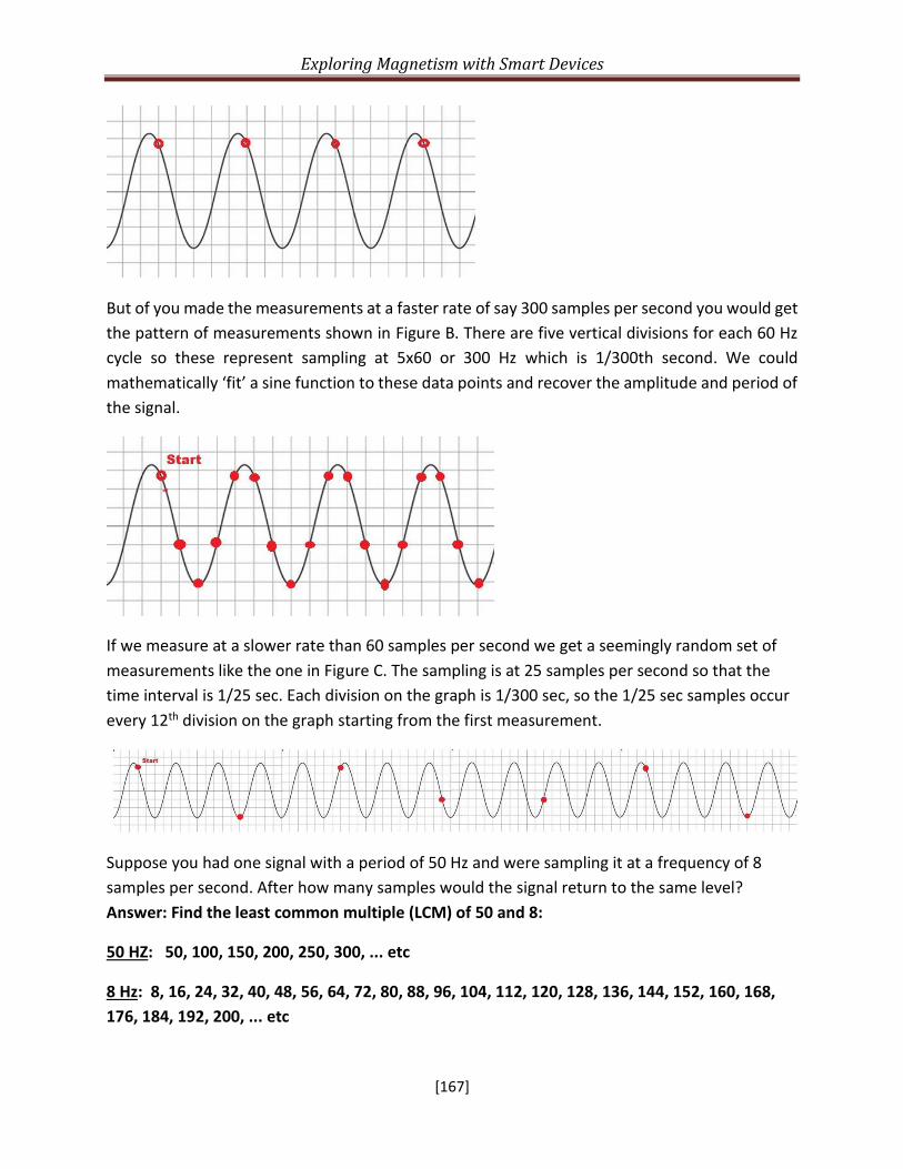
Exploring Magnetism with Smart Devices
[167]
But of you made the measurements at a faster rate of say 300 samples per second you would get
the pattern of measurements shown in Figure B. There are five vertical divisions for each 60 Hz
cycle so these represent sampling at 5x60 or 300 Hz which is 1/300th second. We could
mathematically ‘fit’ a sine function to these data points and recover the amplitude and period of
the signal.
If we measure at a slower rate than 60 samples per second we get a seemingly random set of
measurements like the one in Figure C. The sampling is at 25 samples per second so that the
time interval is 1/25 sec. Each division on the graph is 1/300 sec, so the 1/25 sec samples occur
every 12th division on the graph starting from the first measurement.
Suppose you had one signal with a period of 50 Hz and were sampling it at a frequency of 8
samples per second. After how many samples would the signal return to the same level?
Answer: Find the least common multiple (LCM) of 50 and 8:
50 HZ: 50, 100, 150, 200, 250, 300, ... etc
8 Hz: 8, 16, 24, 32, 40, 48, 56, 64, 72, 80, 88, 96, 104, 112, 120, 128, 136, 144, 152, 160, 168,
176, 184, 192, 200, ... etc
Exploring Magnetism with Smart Devices
[168]
Or by prime factoring: 50 = 2 x 52 and 8 = 23 so LCM = 52 x 23 = 200.
This means that every 200 samples the signal should return to the same measurement as the
first measurement.
Problem 23 – Calculating the height of a cable above the ground
At a distance of 30 meters along the roadway, the cable’s elevation angle is 16o. What is the
height of the cable above the roadway? Answer: Using Trig: Its height above the center of the
roadway is H=30tan(16o) = 7 meters. By construction: Draw a scaled right-triangle with a base
segment AB = 3cm long and the hypothenuse drawn from the vertex at B at an angle of 16o
with a protractor. Draw a perpendicular line at A that intersects the hypothenuse at point C.
Use your ruler to measure the length of segment H= AC and from the scale you used, (1 cm =
10 meters) calculate its length, which is the height of the cable.
Problem 24 – Estimating the current flowing in a distribution line
The equation for the magnetic field of a wire carrying a current, I, is given by:
𝐵 =2𝑥10−7𝐼
𝑅
where I is the current in amperes, R is the distance to the transmission line wire in meters and B
is the resulting magnetic intensity measured by the smart device in Teslas. If |B| =5.1x10⁻⁶
Teslas and R = 7 meters, what is the instantaneous current I? Answer: 180 amperes.
Note: The answer to Problem 37 seems improbably small for a transmission line, however the
strategy for transmitting power long distances while minimizing heat losses from the resistance
of the wire is to use the highest voltage and the lowest current so that P=VxI. Currents in the
range from 200 to 1000 amperes are not unusual.
Problem 25 – Detecting a geomagnetic storm
You made five measurements of a non-storm condition from your phone lying flat on a table
and undisturbed. The values for X, Y and Z are shown in table 13 in columns 1, 2 and 3. During
what was predicted to be the peak of the storm you made five storm-time measurements
shown in table 13 in columns 4, 5 and 6. After the storm had passed you made a final set of five
measurements shown in the table 13 in columns 7, 8 and 9. If your Hall Effect sensor had a
precision of ±0.2 T, how sure are you that you detected the storm event?

Exploring Magnetism with Smart Devices
[169]
The before and after measurements when there was no storm should be averaged together
to get a ‘baseline’ measurement of the quiet field values: X= (24.9+25.1)/2 = 25.0 T; Y=
(1.8+1.6)/2 = 1.7 T; Z= (-46.4 -46.2)/2 = -46.3 T. Now subtract these baseline values from
the storm time values to get X= (26.5-25.0) = +1.5 T; Y= (3.2-1.7) = +1.5 T; Z= (-42.8 + 46.3)
=+3.5 T. The problem stated that the precision of these measurements was ±0.2 T (what
statistically we would call the standard deviation), so for the storm-time measurements, they
are between 7 and 18 times the measurement error. Note: at 3-times the chances are 1 in 750
that the result is due to random error so we can say that the storm event was definitely
detected.
Data Table
1 2 3 4 5 6 7 8 9
Sample X Y Z X Y Z X Y Z
1 24.3 1.7 -46.5 26.4 2.9 -42.8 24.5 1.4 -46.1
2 25.1 1.9 -46.5 26.3 3.2 -43.1 25.1 1.6 -46.3
3 25.3 2.0 -46.2 26.2 3.4 -42.7 25.2 1.5 -46.5
4 25.3 1.8 -46.4 26.7 3.1 -43.3 24.9 1.7 -46.1
5 24.7 1.6 -46.2 26.9 3.2 -42.3 25.8 1.8 -46.2
Average 24.9 1.8 -46.4 26.5 3.2 -42.8 25.1 1.6 -46.2
Problem 26 – How long will I wait for a major geomagnetic storm?
Geomagnetic storms follow the 11-year sunspot cycle. The figure below shows the sunspot
cycles from May 1932 to May 2004 (black line) and the number of days each year when a
severe geomagnetic storm occurred (Kp>= 8).

Exploring Magnetism with Smart Devices
[170]
For the sunspot cycle between May 1986 and May 1997, A) About how many days were there
major geomagnetic storms during sunspot minimum? B) About how long would you have to wait
between these storms? C) During sunspot maximum ca May 1990, about how long would you
have to wait for a severe geomagnetic storm? Answer: A) Sunspot minimum occurred near May
1986 when the red spot indicates there were about 15 days of severe storms. B) You would
have had to wait about 365/15 = 24 days or three weeks. C) The graph shows about 150 days
of severe storms so 365/150 = 3 days. This particular sunspot cycle was one of the most active.
Recent cycles are about 1/3 as active so the estimates times in A, B, C are three times longer
on average.
Problem 27 - Stored energy in an MRI magnet
The MRI magnets for medical imaging have a strength of about 1.5 Teslas. The cylindrical
chamber has dimensions of about 2m long by 1m in diameter. What is the maximum amount of
energy that could be stored in the MRI field if it were uniform throughout the volume?
Answer: Volume = (0.5)2x 2 = 1.6 m3. E = 1.52/(8x10-7) = 0.6 megaJoules or about a
half-stick of dynamite

Exploring Magnetism with Smart Devices
[171]
Problem 28 - Modeling a solar flare event using energy conservation
Below are a set of equations that give the energy in joules of each of these forms.
Magnetic Energy = 107 B2 V /8 where B is in Teslas, V is in m3
Thermal Energy = 3/2 N k T V where N is the gas density in particles/m3, V is the volume in
m3, T is in kelvins and k is Boltzmann constant = 1.38x10⁻²³
Kinetic Energy = ½ m v2 where m is the total mass of the gas cloud in kg, and v is the cloud
speed in m/s.
Gravitational Potential Energy = GMm/r where M is the mass of the sun in kg, m is the mass of
the gas cloud in kg, r is the distance to the cloud from the center of the sun in meters, Newtons
constant of gravity G = 6.67x10⁻¹¹.
A) Suppose a solar flare is produced by the reconnection of a tangled magnetic field at the
surface of the sun and within a volume with an area of 1,000km x 1,000 km and a
thickness of 100 km. Simplify all of the energy equations by evaluating the given
constants, area and volume. The mass and radius of the sun are 2.0x1030kg and 7.0x10⁸
m respectively.
Magnetic Energy = 107 B2 V /8 so Em = 4.0x10²² B2 joules
Thermal Energy = 3/2 N k T V so ET = 2.0x10⁻⁶ NT joules
Gravitational potential energy = GMm/r so Eg= 1.9x10¹¹ m joules.
B) If the magnetic field in the reconnection region has a strength of 0.5 Teslas, what is the
total available magnetic energy available in this volume of space? Answer: Em =
4.0x10²² (0.5)2 = 1.0x10²² joules.
C) The plasma in this volume of space consists of hydrogen (m=1.6x10⁻²⁷ kg) at a density of
2x10⁻⁷ kg/m3, is heated to a temperature of 1,000,000 K. What is the total thermal
energy of the gas? Answer: The gas density N = 2x10⁻⁷/1.6x10-27 = 1.3x10²⁰/m3 then ET
= 2x10⁻⁶)(1.3x10²⁰)(1,000,000) = 2.6x10²⁰ joules.
D) What is the available kinetic energy of the plasma found by subtracting the thermal
energy from the magnetic energy. Answer: E = Em – ET = 2.6x10²⁰ – 1.3x10¹⁹ so the
available energy is E= 2.5x10²⁰ joules.
E) What is the gravitational potential energy of this volume of gas? Answer: mass = 2x10⁻⁷
kg/m3 x (106m x 106m x 105m) = 2x10¹⁰ kg so Eg = 1.9x10¹¹ (2x10¹⁰) = 3.8x10²¹ joules.
F) Does the plasma produced by the reconnection event have enough energy to escape
the solar surface? Answer: No because Eg > E. The plasma only has
100%x(2.5x10²⁰/3.8x1021) = 6.6% of the required escape energy from the solar surface.

Exploring Magnetism with Smart Devices
[172]
Problem 29 - Calculating the magnetic field in a Helmholtz coil.
The strength of the axial magnetic field inside a Helmholtz coil is given by the standards
formula
𝐵 = (4
5)
1.5 𝜇𝑁𝐼
𝑅
where B is the field strength in Tesla, N is the number of loops of wire in each of the coils, I is
the current flowing through the wire in Amperes, and R is the radius in meters of the Helmholtz
coil. The constant has a value of 4x10⁻⁷ so that all units are in the MKS system. For example,
a coil with 20 windings and a radius of 5 cm and I = 0.050 Amperes produces a field
𝐵 = (4
5)
1.5 (1.3𝑥10−6)(20)(0.05)
(0.05)
B = 19.0 T.
A student wants to design a system to cancel part of Earth’s magnetic field, which along
one axis has a value of 25 T. If the coil has a radius of 5 cm, and each coil consists of 20 turns
of wire, what is the minimum current needed to cancel Earth’s field inside the Helmholtz coil?
Answer: R = 0.05 meters; B = 0.000025 Tesla; N = 20 so
𝑰 = (𝟓
𝟒)
𝟏.𝟓 𝑹𝑩
𝝁𝑵
𝑰 = (𝟓
𝟒)
𝟏.𝟓 (𝟎. 𝟎𝟓)(𝟎. 𝟎𝟎𝟎𝟎𝟐𝟓)
(𝟏. 𝟑𝒙𝟏𝟎−𝟔)𝟐𝟎
So I = 0.067 Amperes or 67 milliamps.
A standard D-cell battery can supply 6.5 Amperes for 1 hour. How long can the student keep
this Helmholtz coil operating before the battery dies? Answer: From a simple proportion
(0.067/6.5) = (1 hr/X) so X = (6.5/0.067) = 97 hours.

Exploring Magnetism with Smart Devices
[173]
Problem 30 – Vector dot products and magnetic components
The horizontal component of a magnetic field, vector H, is directed at an angle of 30 degrees to
the axis of a Helmholtz Coil defined by vector C. If |H| = 50 T,
A) Use a geometric construction to calculate the projection of H along the coil’s axis.
B) Use the vector dot product H . C = |H||C| sin where C is the unit vector along the
coil’s axis. Answer: |H| = 50 and |C| = 1.0 because it’s a unit vector, so the dot
product has a magnitude of |HC| = 50sin(30) = 25 T. The projection of H along the
direction of C defines the magnetic component P with |P| = 25 T.

Exploring Magnetism with Smart Devices
[174]
X. Additional NASA resources related to magnetism
Magnetic Math Educator Guide - This collection of mathematics-related problems pertaining to
magnetism is the next logical step beyond what students explore in their middle school Earth science
textbooks. The lab exercises prepare students to work the mathematics problems with a better
understanding of magnetism. The variety of problems includes analyzing graphs, scientific notation,
geometry and trigonometry. The problems call for students to apply mathematics and science concepts
to understand magnetic fields and magnetism. Each one-page assignment includes background
information. One-page answer keys accompany the assignments.
URL: https://www.nasa.gov/stem-ed-resources/magnetic-math.html
Solar System Magnetism - The big idea of this demonstration is that the Sun and Earth have different
magnetic properties. Sunspots are related to magnetism on the Sun. Earth has a strong simple magnetic
field with two poles. The educator builds the magnetic fields using polystyrene spheres, strong magnets
and staples. Then the participants make "field detectors" from simple objects to predict the locations of
the fields.
URL: https://www.nasa.gov/stem-ed-resources/solar-system-magnetism.html
Modeling Earth’s Magnetism - Surrounding Earth is a giant magnetic field called the magnetosphere. Its
shape is defined not only by the planet's north and south magnetic poles, but also by a steady stream of
particles coming in from the sun called the solar wind. The magnetosphere is buffeted by this wind and
can change shape dramatically when the sun lets loose an immense cloud of gas known as a coronal mass
ejection. Credit: NASA's Scientific Visualization Studio
URL: https://solarsystem.nasa.gov/resources/2286/modeling-earths-magnetism/
IMAGE Explores Earth’s Magnetic Field - Welcome to the IMAGE satellite tutorial on Earth's magnetic
field. This page contains a brief introduction to magnetism, and Earth's field. It also provides links to
additional IMAGE reading materials, and a collection of classroom activities that help students
understand Earth's magnetic field and its changes through time and space.
URL: https://image.gsfc.nasa.gov/poetry/magnetism/magnetism.html
Exploring Magnetism: A THEMIS Teachers Guide – This is a guide to magnetism developed for the NASA
THEMIS program through the cooperation of high school teachers participating in the GEONS project. It
covers basic magnetism, Earth’s dynamic magnetic field, and the operating principles of professional-
grade magnetometers for studying geomagnetic storms.
URL: http://cse.ssl.berkeley.edu/SEGwayed/lessons/exploring_magnetism/background/

Exploring Magnetism with Smart Devices
[175]
Jupiter’s Magnetic Field Visualization - A simplified model of Jupiter's massive magnetic field, known as
a magnetosphere. Jupiter's magnetosphere is the largest object in the solar system. If it glowed in
wavelengths visible to the eye, it would appear two to three times the size of the Sun or Moon to viewers
on Earth. In this visualization, the magnetic field structure is represented by gold/copper lines. The semi-
transparent grey mesh in the distance represents the boundary of the magnetosphere. Major satellites of
the planetary system are also included.
URL: https://solarsystem.nasa.gov/resources/1054/jupiters-magnetic-field-visualization/
NASA: Understanding the Magnetic Sun – A visualization of the magnetic field of the sun and its
turbulent nature. The surface of the sun writhes and dances. Far from the still, whitish-yellow disk it
appears to be from the ground, the sun sports twisting, towering loops and swirling cyclones that reach
into the solar upper atmosphere, the million-degree corona – but these cannot be seen in visible light.
Then, in the 1950s, we got our first glimpse of this balletic solar material, which emits light only in
wavelengths invisible to our eyes. Once this dynamic system was spotted, the next step was to understand
what caused it. For this, scientists have turned to a combination of real time observations and computer
simulations to best analyze how material courses through the corona.
URL: https://svs.gsfc.nasa.gov/4623
Sun Magnetic Field Flip Live Shots and Media Resources - On Dec. 6, 2013, NASA scientists Alex Young
and Holly Gilbert discussed how the sun's magnetic field is in the process of flipping. This visualization
shows the position of the sun's magnetic fields from January 1997 to December 2013. The field lines
swarm with activity: The magenta lines show where the sun's overall field is negative and the green lines
show where it is positive. Additional gray lines represent areas of local magnetic variation. The entire sun's
magnetic polarity, flips approximately every 11 years – though sometimes it takes quite a bit longer – and
defines what's known as the solar cycle.
URL: https://svs.gsfc.nasa.gov/11429
CME Week: The Difference Between Flares and CMEs - There are many kinds of eruptions on the sun.
Solar flares and coronal mass ejections both involve gigantic explosions of energy, but are otherwise quite
different. The two phenomena do sometimes occur at the same time – indeed the strongest flares are
almost always correlated with coronal mass ejections – but they emit different things, they look and travel
differently, and they have different effects near planets.
URL: https://www.nasa.gov/content/goddard/the-difference-between-flares-and-cme

Exploring Magnetism with Smart Devices
[176]

NP-2021-10-697-GSFC
National Aeronautics and Space Administration NASA Heliophysics Education Activation Team
Goddard Space Flight Center Greenbelt, MD 20771 https://go.nasa.gov/2IXhsFq