exploring portfolio scheduling for long-term execution of scientific

Exploring Portfolio Scheduling for Long-term Execution ofScientific Workloads in IaaS Clouds

Kefeng Deng, Junqiang Song, Kaijun RenSchool of Computer

National University of Defense TechnologyChangsha, China

{dengkefeng,junqiang,renkaijun}@nudt.edu.cn

Alexandru IosupParallel and Distributed Systems Group

Delft University of TechnologyDelft, The [email protected]

ABSTRACTLong-term execution of scientific applications often leads todynamic workloads and varying application requirements.When the execution uses resources provisioned from IaaSclouds, and thus consumption-related payment, efficientand online scheduling algorithms must be found. Portfolioscheduling, which selects dynamically a suitable policy froma broad portfolio, may provide a solution to this problem.However, selecting online the right policy from possiblytens of alternatives remains challenging. In this work,we introduce an abstract model to explore this selectionproblem. Based on the model, we present a comprehensiveportfolio scheduler that includes tens of provisioning andallocation policies. We propose an algorithm that canenlarge the chance of selecting the best policy in limitedtime, possibly online. Through trace-based simulation, weevaluate various aspects of our portfolio scheduler, and findperformance improvements from 7% to 100% in comparisonwith the best constituent policies and high improvement forbursty workloads.

Categories and Subject DescriptorsC.2.4 [Distributed Systems]: Distributed Applications

General TermsAlgorithms, Economics, Management, Performance

KeywordsPortfolio Scheduling, Resource Provisioning, IaaS Cloud,Scientific Workloads

1. INTRODUCTIONThe past few years have seen a growing number of

scientific computing communities evaluating IaaS clouds forrunning scientific workloads. For example, several usershave tried virtual clusters built with resources leased from

Permission to make digital or hard copies of all or part of this work forpersonal or classroom use is granted without fee provided that copies are notmade or distributed for profit or commercial advantage and that copies bearthis notice and the full citation on the first page. Copyrights for componentsof this work owned by others than ACM must be honored. Abstracting withcredit is permitted. To copy otherwise, or republish, to post on servers or toredistribute to lists, requires prior specific permission and/or a fee. Requestpermissions from [email protected] November 17-21 2013, Denver, CO, USAhttp://dx.doi.org/10.1145/2503210.2503244.

commercial clouds such as Amazon EC2 [11, 17]. Othercommunities have converted their local clusters into publicor private clouds [16, 42]. Taking advantages of IaaS cloudresources could hold great promise for scientific computing,especially for highly variable workloads and for parallel jobswhich otherwise would have to wait in production queues forlong periods of time. To achieve this promise, both scientistsand cloud operators still need efficient scheduling algorithmsfor resource provisioning and job allocation. Although manyscheduling algorithms already exist and many have beenadapted for IaaS clouds, several studies have shown thatnone of these algorithms is able to perform well across a widevariety of scientific workload characteristics. To alleviate theproblem of selecting a scheduling algorithm, in this workwe explore the concept of portfolio scheduling, that is, ofselecting a suitable policy from a portfolio, with time limitsfor the selection process.

Scheduling demanding scientific workloads in the cloud isnontrivial. Genaud et al. [10, 27] study bin-packing strate-gies for scheduling independent, sequential grid workloads inIaaS clouds. Marshall et al. [25] and Wang et al. [43] presentresource provisioning policies for parallel jobs in order to bal-ance monetary cost and job wait time. Other efforts focusedon cost-efficient execution of applications such as Bags-of-Tasks (BoTs) [2,28] and scientific workflows [21,22]. To gaindeep insight into the performance of scheduling policies, ourprevious work [41] studies the interplay between provisioningand allocation policies through real experiments. Matchingprevious studies [13, 14, 35], the results show that no onepolicy performs the best in all possible situations.

Instead of striving to find better individual schedulingpolicies, our previous research [8] adapted portfolio schedul-ing [12] to scientific workloads running in IaaS clouds. Thebasic idea of portfolio scheduling is to construct a portfolioof scheduling policies, and to select from it the most suitablepolicy for the current workload and system conditions.The portfolio scheduler evaluates the relative performanceof constituent policies though an online, discrete-eventsimulator. Our previous results have shown that portfolioscheduling can be a viable solution for various workloadpatterns that include small parallel jobs.

Significantly extending our previous work, in this articlewe explore a variety of methods not only to reduce theoverhead of portfolio scheduling but also to improve thequality of portfolio selection. In comparison with ourprevious work on portfolio scheduling, we adapt it here fora more demanding and general application model, that is,the long-term execution of small- and medium-scale parallel

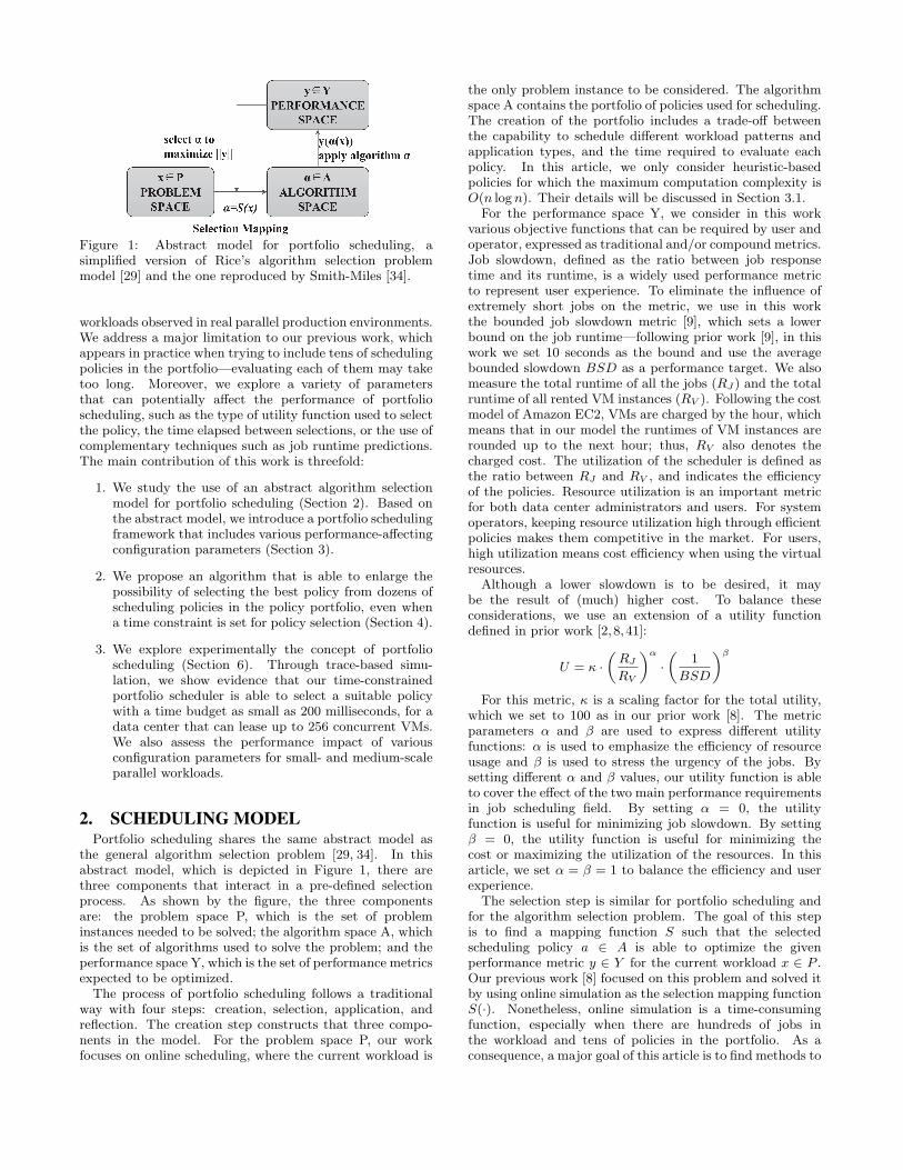
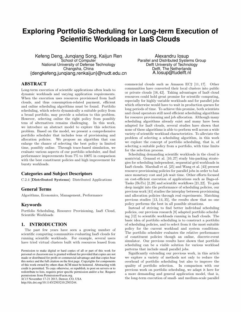
Figure 1: Abstract model for portfolio scheduling, asimplified version of Rice’s algorithm selection problemmodel [29] and the one reproduced by Smith-Miles [34].

workloads observed in real parallel production environments.We address a major limitation to our previous work, whichappears in practice when trying to include tens of schedulingpolicies in the portfolio—evaluating each of them may taketoo long. Moreover, we explore a variety of parametersthat can potentially affect the performance of portfolioscheduling, such as the type of utility function used to selectthe policy, the time elapsed between selections, or the use ofcomplementary techniques such as job runtime predictions.The main contribution of this work is threefold:

1. We study the use of an abstract algorithm selectionmodel for portfolio scheduling (Section 2). Based onthe abstract model, we introduce a portfolio schedulingframework that includes various performance-affectingconfiguration parameters (Section 3).

2. We propose an algorithm that is able to enlarge thepossibility of selecting the best policy from dozens ofscheduling policies in the policy portfolio, even whena time constraint is set for policy selection (Section 4).

3. We explore experimentally the concept of portfolioscheduling (Section 6). Through trace-based simu-lation, we show evidence that our time-constrainedportfolio scheduler is able to select a suitable policywith a time budget as small as 200 milliseconds, for adata center that can lease up to 256 concurrent VMs.We also assess the performance impact of variousconfiguration parameters for small- and medium-scaleparallel workloads.

2. SCHEDULING MODELPortfolio scheduling shares the same abstract model as

the general algorithm selection problem [29, 34]. In thisabstract model, which is depicted in Figure 1, there arethree components that interact in a pre-defined selectionprocess. As shown by the figure, the three componentsare: the problem space P, which is the set of probleminstances needed to be solved; the algorithm space A, whichis the set of algorithms used to solve the problem; and theperformance space Y, which is the set of performance metricsexpected to be optimized.The process of portfolio scheduling follows a traditional

way with four steps: creation, selection, application, andreflection. The creation step constructs that three compo-nents in the model. For the problem space P, our workfocuses on online scheduling, where the current workload is

the only problem instance to be considered. The algorithmspace A contains the portfolio of policies used for scheduling.The creation of the portfolio includes a trade-off betweenthe capability to schedule different workload patterns andapplication types, and the time required to evaluate eachpolicy. In this article, we only consider heuristic-basedpolicies for which the maximum computation complexity isO(n logn). Their details will be discussed in Section 3.1.

For the performance space Y, we consider in this workvarious objective functions that can be required by user andoperator, expressed as traditional and/or compound metrics.Job slowdown, defined as the ratio between job responsetime and its runtime, is a widely used performance metricto represent user experience. To eliminate the influence ofextremely short jobs on the metric, we use in this workthe bounded job slowdown metric [9], which sets a lowerbound on the job runtime—following prior work [9], in thiswork we set 10 seconds as the bound and use the averagebounded slowdown BSD as a performance target. We alsomeasure the total runtime of all the jobs (RJ) and the totalruntime of all rented VM instances (RV ). Following the costmodel of Amazon EC2, VMs are charged by the hour, whichmeans that in our model the runtimes of VM instances arerounded up to the next hour; thus, RV also denotes thecharged cost. The utilization of the scheduler is defined asthe ratio between RJ and RV , and indicates the efficiencyof the policies. Resource utilization is an important metricfor both data center administrators and users. For systemoperators, keeping resource utilization high through efficientpolicies makes them competitive in the market. For users,high utilization means cost efficiency when using the virtualresources.

Although a lower slowdown is to be desired, it maybe the result of (much) higher cost. To balance theseconsiderations, we use an extension of a utility functiondefined in prior work [2,8, 41]:

U = κ ·(RJ

RV

)α

·(

1

BSD

)β

For this metric, κ is a scaling factor for the total utility,which we set to 100 as in our prior work [8]. The metricparameters α and β are used to express different utilityfunctions: α is used to emphasize the efficiency of resourceusage and β is used to stress the urgency of the jobs. Bysetting different α and β values, our utility function is ableto cover the effect of the two main performance requirementsin job scheduling field. By setting α = 0, the utilityfunction is useful for minimizing job slowdown. By settingβ = 0, the utility function is useful for minimizing thecost or maximizing the utilization of the resources. In thisarticle, we set α = β = 1 to balance the efficiency and userexperience.

The selection step is similar for portfolio scheduling andfor the algorithm selection problem. The goal of this stepis to find a mapping function S such that the selectedscheduling policy a ∈ A is able to optimize the givenperformance metric y ∈ Y for the current workload x ∈ P .Our previous work [8] focused on this problem and solved itby using online simulation as the selection mapping functionS(·). Nonetheless, online simulation is a time-consumingfunction, especially when there are hundreds of jobs inthe workload and tens of policies in the portfolio. As aconsequence, a major goal of this article is to find methods to

Figure 2: The framework of our portfolio scheduler, aconcrete realization of the abstract scheduling model.

reduce the overhead of portfolio simulation while preservingthe quality of the selection.In the application step, the policy that can maximize the

utility function in the performance space Y is selected andapplied to make real scheduling decisions. The performanceof the scheduling policy is collected and stored in thedatabase for reflection. By analyzing the performance ofthe past selected policies, the reflection step could be usefulfor improving the quality of selection for future workloads.We further parameterize the model introduced in this

section with an interval between selection decisions and witha time constraint for selecting policies.

3. PORTFOLIO SCHEDULEROur portfolio scheduler is a concrete realization of the

abstract scheduling model discussed in previous section.We design a framework for portfolio scheduling, depictedin Figure 2. The component “Policy Portfolio” implementsthe algorithm space A, which provides dozens of alternativepolicies for the online simulator. The“online simulator”usesthe provided scheduling policy to run in simulation the jobscurrently in the “Job Queue”, based on the resource profileof current system; the result of the simulation is a utilityscore for each evaluated policy. Possibly aided by historicalperformance data, the “policy selector” chooses the mostsuitable policy according to the selected reflection criterion.In the remainder of this section, we present the components“Policy Portfolio”, the “Runtime Predictor”, and the “OnlineSimulator”, in turn.

3.1 The Policy PortfolioSimilarly to our previous work [8, 41], we break the

scheduling policies into three parts: the provisioning poli-cies, the job selecting policies and the VM selecting policies.To run the queued jobs, the scheduling policy first provisionsa suitable number of VMs from the cloud through theresource provisioning policy, then uses the job selectingpolicy to order the queued jobs; for each selected job, itselects the required number of appropriate VMs from thecloud according to the VM selecting policy. We populate theportfolio with policies chosen from research work on resourceprovisioning and scheduling of parallel jobs.Five provisioning policies are used in our portfolio sched-

uler. They consider the job wait time (qi for job i), thejob runtime (ti for job i), and the job parallelism (ni, thenumber of processors requested by job i):

1. (The baseline policy) On-Demand All (ODA): Thisis a simple, commonly used policy [8, 10, 25, 27, 41]. Itleases the required number of VMs for all the queuedjobs whenever there are available VMs. This policyis naive: although it may lead to low job slowdown, italso incurs unnecessarily high cost as resources chargedfor an entire hour may be released after just a fewminutes of use.

2. On-Demand Balance (ODB): Because scientific work-loads may include many short jobs that finish beforethe hourly charging of resources, it is not necessary torent new instances for every job. Therefore, the ODBpolicy tries to keep equal (balanced) the total numberof required processors and the number of processorsthat have already rented. This policy is very similarto the resource management policy presented by theDawningCloud [43].

3. On-Demand ExecTime (ODE): The ODE policy is anextension for parallel jobs of the ODE policy we haveused in our previous work [8, 41]. It calculates thenumber of required VMs by rounding the total runtimeof all the queued jobs into hours:

∑ni · ti/3600. The

intuition is to pack the jobs as tightly as possible inorder to minimize the cost.

4. On-Demand Maximum (ODM): This policy leases themaximum number of VMs requested by jobs currentlyin the queue: max (n1, n2, . . .). ODM ensures thatat least one queued job can be started. The policyis helpful when most of the queued jobs are short,because they can run on already rented VMs insteadof leasing new VMs (the ODA policy).

5. On-Demand XFactor (ODX): The ODX policy isdirectly taken from our previous work [8, 41]. It rentsthe required number of VMs for every job once its

bounded slowdown qi+max(ri,10)max(ri,10)

exceeds a threshold

of 2. This policy can lead to a good trade-off betweenuser experience and resource utilization.

The job selection first orders the job queue based onpriority functions, then chooses the first job of the queuefor scheduling until insufficient resources remain available.Many job selection policies have been proposed in theliterature for various types of jobs. Tan et al. [39] proposeseveral policies that compute job priority (pi) based on threefactors: job wait time, job run time, and job parallelism.Since their proposed policies cover a wide range of policiesused in the literature and can avoid job starvation, they arechosen as the candidate job selection policies in our policyportfolio:

1. (The baseline policy) First-Come-First-Serve (FCF-S): FCFS uses the priority : pi = qi, to order thewaiting jobs. This policy is the most commonly usedpolicy for parallel job scheduling and is taken as thebaseline policy for job selection.

2. Largest-Slowdown-First (LXF): LXF orders the jobqueue by the slowdown of the jobs: pi = (qi+ti)/ti. Incomparison with FCFS, this policy also considers jobrun time. The intuition is that short jobs suffer morefrom long wait time than long jobs.

3. WFP3: Unlike LXF, which may delay large-scale jobsfor a long time, WFP3 takes job parallelism intoconsideration and prioritizes the job queue by function:pi = (qi/ti)

3 · ni. In addition to preferring large jobs,WFP3 puts more weight on job slowdown since thefirst factor is cubed.

4. UNICEF: In comparison with WFP3, UNICEF goes tothe other extreme, by preferring small-scale jobs withshort run time. This policy sorts the job queue basedon the priority: pi = qi/ (log2(ni) · ti). It tries to offerquick response time for small jobs.

Although we lease one type of VMs for all the jobs, thereis still a need to choose a proper set of VMs for eachselected job. The reason is that idle VMs may have differentremaining time until they get charged for the next hour.Based on different consideration of the remaining time, weuse for VM selection three policies that are originally usedto solve the online bin-packing problem [6,10]:

1. (The baseline policy) First Fit (FF): FF is thesimplest VM selection policy in our study. FF choosesidle VMs without distinction. The advantage of thispolicy is speed, especially in comparison to policiesthat sort the VMs.

2. Best Fit (BF): For each selected job, BF chooses theVMs such that the remaining time of the selectedVMs after running the job is minimal across availableVMs. This policy aims at reducing the charged costby improving the utilization of the VMs.

3. Worst Fit (WF): Conversely, WF selects the VMs thatwill have the maximum remaining time after runningthe job. The goal of this policy is to balance the usageof each VM. By leaving as much idle time as possible,a large job arriving in the future may be more easilyallocated to existing VMs.

Overall, we get a total of 60 scheduling policies in ourpolicy portfolio. Given m jobs and n VMs, the maximumcomputation complexity of VM provisioning is O(m) andthe maximum computation complexity for job allocation isO(m logm) · O(n logn). Thus, the maximum computationcomplexity of the scheduling policies is O(mn logmn).

3.2 The Runtime PredictorJob runtime is an indispensable information in our port-

folio scheduler, not only because it is used in some ofthe resource provisioning and job selection policies, butalso for the simulation of policies by the online simulator(see Section 3.3). Though users are required to provideestimated runtime for their jobs in many computer systems,their estimates are known to be highly inaccurate [40,44]. Therefore, Tsafrir et al. [40] suggest replacing userestimates with system-generated predictions for parallel jobscheduling. In particular, they use the average runtime ofthe two most recently submitted and completed jobs fromthe same user as the predicted runtime for the new job.In our portfolio scheduler, we use the algorithm suggested

by Tsafrir et al. [40] to adjust user estimates. The algorithmis an instance of the widely used k-nearest neighbor (k-nn)algorithm [33]. Experimental results have shown k=2 is theoptimal operation window for the evaluated workloads with

an accuracy around 50% [36, 40]. A thorough study of jobruntime prediction is beyond the scope of this work; werefer to [26] for more sophisticated algorithms. Nevertheless,the experimental results in Section 6.3 show that even forsuch an inaccurate predictor, our portfolio scheduler can stillperform well.

3.3 The Online SimulatorThe online simulator represents the selection mapping

between the scheduling policy and the performance targetin the abstract scheduling model introduced in Section 2.We implement the simulator as a function of the queuedworkload (the queued jobs), the cloud profile (the informa-tion of running and idle VMs in the current system), andthe scheduling policy. The simulator uses the schedulingpolicy for resource provisioning and allocation until all thejobs in the workload are finished. After that, it outputs theutility score of the scheduling policy and the simulation cost.This process continues until all the scheduling policies areevaluated or a time condition interrupts the process.

As mentioned previously, online simulation is an expensivemapping function. For tens of scheduling policies in asingle portfolio, the time taken to evaluate all of them couldbe prohibitive—when the number of queued jobs and ofcandidate VMs is in the order of hundreds to thousands,the portfolio scheduler cannot take sub-second decisions.To solve this problem, we introduce a time constraint andpresent a time-constrained portfolio simulation algorithm tolimit the execution of the online simulator in the followingsection.

4. TIME-CONSTRAINED SIMULATIONTo make sure the scheduling decisions are made in time,

we set a constraint ∆ to limit the time spent for any singlesimulation of the entire portfolio. To maximize the chanceof selecting the best policy for the current workload, wecategorize the scheduling policies into three sets: Smart,Stale and Poor. The policies in the Smart set haveobtained top utility-function scores in the previous portfoliosimulation. The policies in the Pool set have performedthe worst in the former simulation. The Stale set containspolicies from the Smart set and the Poor set that have notbeen simulated in the previous simulation.

We design an algorithm for portfolio scheduling with timeconstraints that uses the three sets of policies Smart, Stale,and Poor. Algorithm 1 summarizes the pseudo-code of thealgorithm, which includes three phases. The first phaseallocates time quotas for the three sets. As shown byAlgorithm 1 line 1-2, ∆ is first partitioned proportionallyto the number of policies in Smart, Stale and Poor. Whenthe algorithm is first invoked, all the policies are put intoSmart set. Hence, both Stale and Poor are empty, andSmart gets the entire ∆ time for simulation.

The second phase simulates the sets of policies under thelimitation of their time quotas (Algorithm 1 line 3-19). Thepolicies in Smart, Stale, and Poor are simulated, in thisorder. The procedure simulate receives as input the queueof batch jobs (Queue), the resource state of current cloud(Profile), and the scheduling policy (Pi); simulate returnsthe utility score of the scheduling policy (si) along with thesimulation time (ci). For Smart and Stale, the policies aresimulated sequentially until their quotas run out. For Poor,the algorithm randomly selects a policy, each time. All the

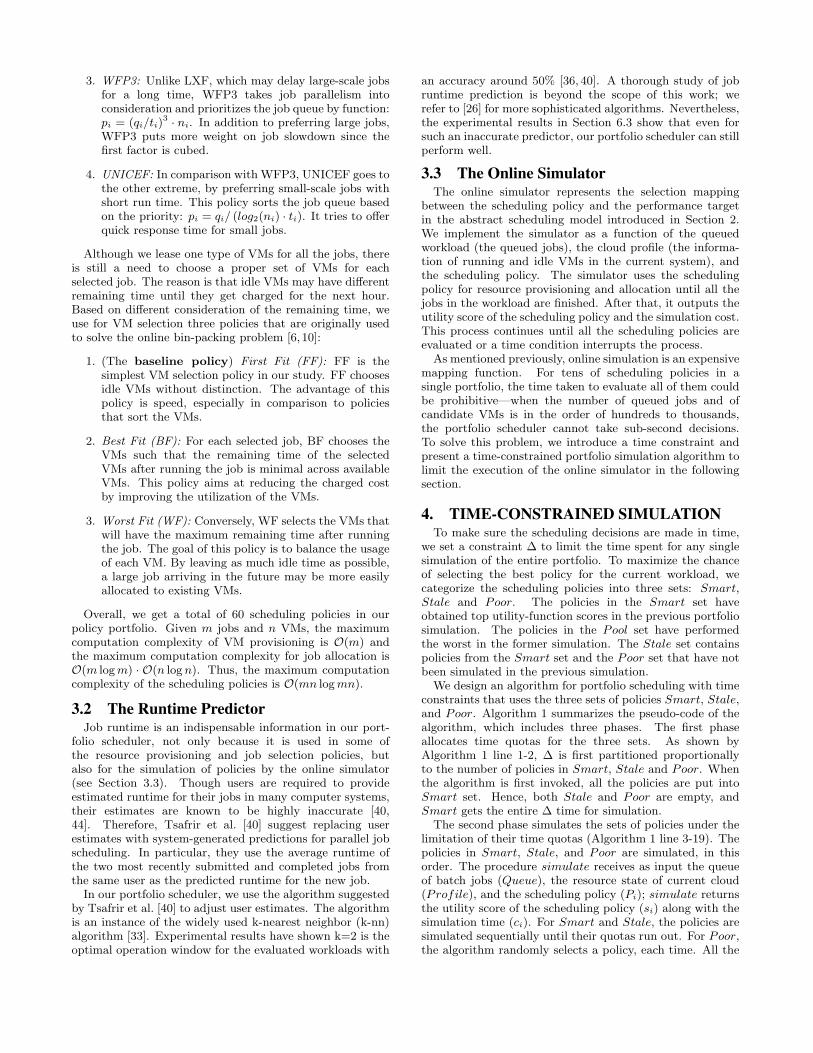
Algorithm 1 Time-Constrained Portfolio Simulation

Input: Queue, the set of batch jobs; Profile, the state ofcurrent system; Smart, the set of smart policies; Stale,the set of stale policies; Poor, the set of poor policies;λ, the selection ratio

Output: The best policy for current workload

1: Q← ∅, N = ∥Smart∥+ ∥Stale∥+ ∥Poor∥;2: δ1 = ∥Smart∥

N·∆, δ2 = ∥Stale∥

N·∆, δ3 = ∆− (δ1 + δ2);

3: for Pi ∈ Smart, i = 1, 2, · · · , ∥Smart∥ && δ1 > 0 do4: si, ci = simulate(Queue, Profile, Pi);5: Smart← Smart− {Pi}, Q← Q ∪ {Pi};6: δ1 = δ1 − ci;7: end for8: for Pi ∈ Stale, i = 1, 2, · · · , ∥Stale∥ && δ2 > 0 do9: si, ci = simulate(Queue, Profile, Pi);10: Stale← Stale− {Pi}, Q← Q ∪ {Pi};11: δ2 = δ2 − ci;12: end for13: δ3 = δ3 + δ2 + δ1;14: while δ3 > 0 do15: i = Random.nextInt(∥Poor∥);16: si, ci = simulate(Queue, Profile, Pi);17: Poor ← Poor − {Pi}, Q← Q ∪ {Pi};18: δ3 = δ3 − ci;19: end while20: Stale← Stale ∪ Smart, Smart← ∅;21: Selector.sort(Q);22: Smart← {Pi ∈ Q|i = 1, 2, · · · , λ∥Q∥};23: Poor ← Poor ∪ {Q− Smart};24: return Smart.first();

simulated policies are moved out from their original sets andput into a temporary set Q.The final phase is to rearrange the policies and return the

best policy for scheduling the current workload (Algorithm 1line 20-24). Firstly, the remaining policies in Smart areput into the end of Stale such that the policies in Staleare simulated in accordance to their staleness. After that,the algorithm calls Selector procedure, which sorts thesimulated policies based on their utility score and puts thetop λ∥Q∥ policies into Smart. The remaining (1 − λ)∥Q∥policies, which had exhibited lower performance in the onlinesimulator, are added into the Poor set. The score of thesimulated policies is also stored in the database for reflection,which we will explore in the future work. Since the firstpolicy in Smart has the highest performance, it is selectedas the best policy and returned to portfolio scheduler forreal scheduling.Our algorithm has an stabilization property: the num-

ber of policies in each set will approximately stabilize at∥Smart∥ = λK, ∥Stale∥ = λ(N − K), and ∥Poor∥ =(1 − λ)N . We now provide an informal proof. Assumethat an average of K policies can be simulated in thegiven time constraint ∆. Thus, for a single policy, it takesµ = ∆

Ktime to be simulated. After the first invocation of

Algorithm 1, there will be λK, (1−λ)K and (N−K) policiesin Smart, Poor and Stale respectively. In the secondinvocation, Quota = λK

N∆ time is allocated to Smart, and

Quotaµ

policies will be simulated. This means λK(1 − KN)

policies will be removed from Smart and put into Stale.Suppose at a particular time, Stale contains x policies.

Sep 1996 Mar 1997 Aug 19970

20

40

60

80

100

# of Submitted Jobs

(a) KTH-SP2

Apr 1998 Apr 1999 Apr 20000

20

40

60

80

100

# of Submitted Jobs

(b) SDSC-SP2

Jan 2003 Jul 2003 Jan 20040

20

40

60

80

100

# of Submitted Jobs

(c) DAS2-fs0

Aug 2004 Dec 2004 May 20050

20

40

60

80

100

# of Submitted Jobs

(d) LPC-EGEE

Figure 3: The number of submitted jobs during ten-minuteintervals in four small-to-medium parallel computer systems.All traces show distinct workload patterns. The vertical axisis limited to 100 for better visibility.

Table 1: The characteristics of the workload traces,including the total number of jobs, the number of jobs thatrequire no more than 64 processors (count and percentage).

Trace#. NameTime[mo.]

JobsCPUs

Load[%]− ≤ 64 %

T1. KTH SP2 11 28,480 28,158 98.9 100 70.4T2. SDSC SP2 24 53,911 53,548 99.3 128 83.5T3. DAS2 fs0 12 215,638 206,925 96.0 144 14.9T4. LPC-EGEE 9 214,322 214,322 100 140 20.8

Then, Quota = ∆Nx time is allocated to Stale by which

KNx policies will be simulated and removed. Among the

simulated policies, the well-performing policies will be putinto Smart and the poorly performing policies will be placedinto Poor. This process will continue until K

Nx is equivalent

to λK(1− KN), or x = λ(N −K).

As a consequence of the stabilization property, for sub-sequent invocations the effect of Algorithm 1 is to verifythe goodness of the previously well-performed policies inSmart, then simulate the oldest policies in Stale, andthen attempt to possibly select a good policy in Poor, bychance. Importantly yet counter-intuitively, a policy in Poorcan still deliver excellent performance in the future—it issufficient that the workload changes in a way that plays tothe strengths of this policy. In the scheduler, we set λ = 0.6,which means the top 60% of the simulated policies will beput into Smart and the other 40% will be put into Poor.The setting is kept constant throughout the experiments andwe will explore its impact in our future work.

5. EXPERIMENTAL SETUPIn this study, we use trace-based simulation to assess

our portfolio scheduler and the proposed algorithm fortime-constrained portfolio scheduling. We now present thesimulator and the workload traces used for our experiments.

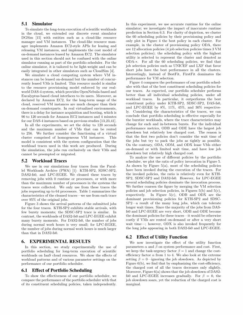
5.1 SimulatorTo simulate the long-term execution of scientific workloads

in the cloud, we extended our discrete event simulatorDGSim [15] with entities such as a cloud-like resourcemanager and VM instances. The cloud-like resource man-ager implements Amazon EC2-style APIs for leasing andreleasing VM instances, and implements the cost model ofon-demand instances leased by Amazon EC2. The simulatorused in this section should not be confused with the onlinesimulator running as part of the portfolio scheduler. For theonline simulator, it is tailored to be light-weight and can beeasily integrated in other simulators such as CloudSim [4].We simulate a cloud computing system where VM in-

stances can be leased on-demand but the number of concur-rently leased VMs is limited. This resource model is similarto the resource provisioning model enforced by our real-world DAS-4 system, which provides OpenNebula-based andEucalyptus-based cloud interfaces to its users. Moreover, asdeclared by Amazon EC2, for the long-term usage of thecloud, reserved VM instances are much cheaper than theiron-demand counterparts. In real virtualized environments,there is a delay for instance acquisition and booting, which is90 to 120 seconds for Amazon EC2 instances and 4 minutesfor our DAS-4 instances based on previous studies [13,23,41].In all the experiments, we set the delay to 120 seconds

and the maximum number of VMs that can be rentedto 256. We further consider the functioning of a virtualcluster comprised of homogeneous VM instances. Thismodel is consistent with the system configuration that theworkload traces used in this work are produced. Duringthe simulation, the jobs run exclusively on their VMs andcannot be preempted or migrated.

5.2 Workload TracesWe use in our simulations four traces from the Paral-

lel Workloads Archive (PWA) [1]: KTH-SP2, SDSC-SP2,DAS2-fs0, and LPC-EGEE. We cleaned these traces byremoving jobs with 0 runtime or processors, or with morethan the maximum number of processors in the systems thetraces were collected. We only use from these traces thejobs requesting up to 64 processors. Table 1 summarizes thecharacteristics of the cleaned traces—we use from each traceover 95% of the original jobs.Figure 3 shows the arrival patterns of the submitted jobs

for the four traces. KTH-SP2 exhibits stable arrivals, withfew bursty moments; the SDSC-SP2 trace is similar. Incontrast, the workloads of DAS2-fs0 and LPC-EGEE exhibitmany bursty moments. For DAS2-fs0, the number of jobsduring normal work hours is very small; for LPC-EGEE,the number of jobs during normal work hours is much largerthan that in DAS2-fs0.

6. EXPERIMENTAL RESULTSIn this section, we study experimentally the use of

portfolio scheduling for long-term execution of scientificworkloads on IaaS cloud resources. We show the effects ofworkload patterns and of various parameter settings on theperformance of our portfolio scheduler.

6.1 Effect of Portfolio SchedulingTo show the effectiveness of our portfolio scheduler, we

compare the performance of the portfolio scheduler with thatof its constituent scheduling policies, taken independently.

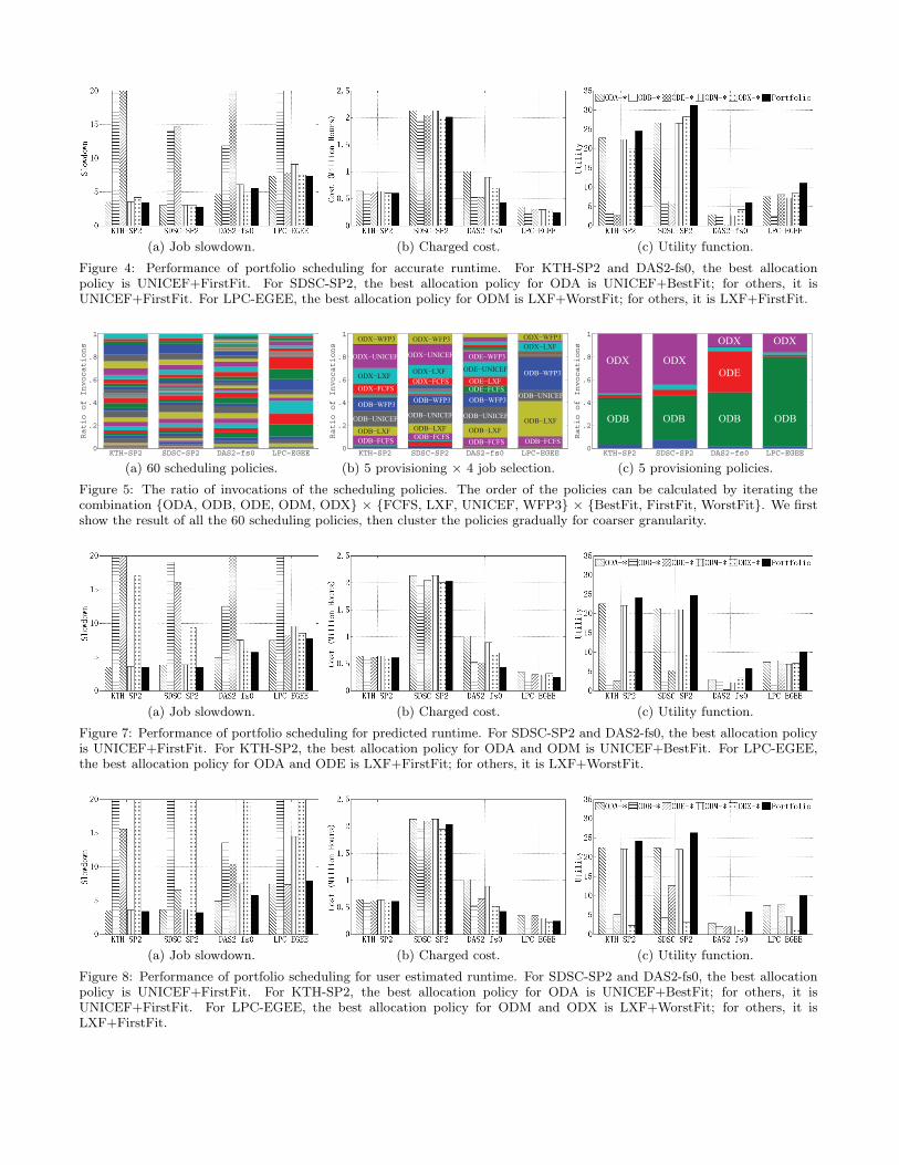
In this experiment, we use accurate runtime for the onlinesimulator; we investigate the impact of inaccurate runtimeprediction in Section 6.3. For clarity of depiction, we clusterthe 60 scheduling policies by their provisioning policy andonly plot in Figure 4 the best policy in each cluster. Forexample, in the cluster of provisioning policy ODA, thereare 12 allocation policies (4 job selection policies times 3 VMselection policies); the scheduling policy with the highestutility is selected to represent the cluster and denoted asODA-∗. For all the 60 scheduling policies, we find thatjob selection policies such as UNICEF and LXF that favorshort jobs have the best performance in all the clusters.Interestingly, instead of BestFit, FirstFit dominates theperformance for VM selection.

Figure 4 compares the performance of our portfolio sched-uler with that of the best constituent scheduling policies forour traces. As expected, our portfolio scheduler performsbetter than all individual scheduling policies, under allworkload traces. In particular, it outperforms the bestconstituent policy under KTH-SP2, SDSC-SP2, DAS-fs0,and LPC-EGEE by 8%, 11%, 45%, and 30% respective-ly. Considering the characteristics of the traces, we canconclude that portfolio scheduling is effective especially forthe burstier workloads, where the trace characteristics maychange for each and in-between bursts. For the individualperformance metrics, ODB and ODE have the largest jobslowdown but relatively low charged cost. The reason isthat the first two policies don’t consider the wait time ofthe jobs but try to pack the jobs as tightly as possible.On the contrary, ODA, ODM, and ODX lease VMs eitheron-demand or with limited wait time, and have low jobslowdown but relatively high charged cost.

To analyze the use of different policies by the portfolioscheduler, we plot the ratio of policy invocation in Figure 5.As shown by Figure 5(a), most of the scheduling policieshave been invoked during the execution of the traces. Forthe invoked policies, the ratio is relatively even for KTH-SP2, SDSC-SP2 and DAS2-fs0. However, for LPC-EGEEseveral scheduling policies dominate the invocation process.We further coarsen the figure by merging the VM selectionpolicies and job selection policies, in Figures 5(b) and 5(c),respectively. In Figure 5(c), ODB and ODX are thedominant provisioning policies for KTH-SP2 and SDSC-SP2—a result of the many long jobs, which can toleratelonger wait times. Since the majority of the jobs from DAS-fs0 and LPC-EGEE are very short, ODB and ODE becomethe dominant policies for these traces—it would be otherwisecostly if VMs are rented on-demand or after a very shortwait time—; however, ODX is also invoked frequently forthe long jobs appearing in both DAS2-fs0 and LPC-EGEE.

6.2 Effect of Utility FunctionWe now investigate the effect of the utility function

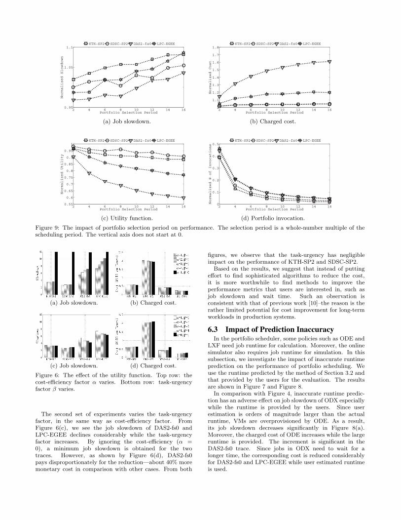
parameters α and β on system performance and cost. First,we keep the task-urgency factor β = 1 and change the cost-efficiency factor α from 1 to 4. We also look at the extremesetting β = 0—ignoring the job slowdown. As depicted byFigure 6(b), we find that by emphasizing the cost-efficiency,the charged cost of all the traces decreases only slightly.Moreover, Figure 6(a) shows that the job slowdown of DAS2-fs0 and LPC-EGEE increases gradually. For β = 0, thejob slowdown soars, yet the reduction of the charged cost ismarginal.

(a) Job slowdown. (b) Charged cost. (c) Utility function.

Figure 4: Performance of portfolio scheduling for accurate runtime. For KTH-SP2 and DAS2-fs0, the best allocationpolicy is UNICEF+FirstFit. For SDSC-SP2, the best allocation policy for ODA is UNICEF+BestFit; for others, it isUNICEF+FirstFit. For LPC-EGEE, the best allocation policy for ODM is LXF+WorstFit; for others, it is LXF+FirstFit.

KTH−SP2 SDSC−SP2 DAS2−fs0 LPC−EGEE0

.2

.4

.6

.8

1

Ratio of Invocations

(a) 60 scheduling policies.


.2

.4

.6

.8

1Ratio of Invocations

ODB−FCFS

ODB−LXF

ODB−UNICEF

ODB−WFP3

ODX−WFP3

ODX−UNICEF

ODX−LXF

ODX−FCFS

ODB−FCFS

ODB−LXF

ODB−UNICEF

ODB−WFP3

ODX−WFP3

ODX−UNICEF

ODX−LXF

ODX−FCFS

ODB−FCFS

ODB−LXF

ODB−UNICEF

ODB−WFP3

ODE−WFP3

ODE−UNICEF

ODE−LXF

ODE−FCFS

ODB−FCFS

ODB−LXF

ODB−UNICEF

ODB−WFP3

ODX−WFP3

ODX−LXF

(b) 5 provisioning × 4 job selection.


.2

.4

.6

.8

1

Ratio of Invocations

ODB

ODX

ODB

ODX

ODB

ODE

ODX

ODB

ODX

(c) 5 provisioning policies.

Figure 5: The ratio of invocations of the scheduling policies. The order of the policies can be calculated by iterating thecombination {ODA, ODB, ODE, ODM, ODX} × {FCFS, LXF, UNICEF, WFP3} × {BestFit, FirstFit, WorstFit}. We firstshow the result of all the 60 scheduling policies, then cluster the policies gradually for coarser granularity.


Figure 7: Performance of portfolio scheduling for predicted runtime. For SDSC-SP2 and DAS2-fs0, the best allocation policyis UNICEF+FirstFit. For KTH-SP2, the best allocation policy for ODA and ODM is UNICEF+BestFit. For LPC-EGEE,the best allocation policy for ODA and ODE is LXF+FirstFit; for others, it is LXF+WorstFit.


Figure 8: Performance of portfolio scheduling for user estimated runtime. For SDSC-SP2 and DAS2-fs0, the best allocationpolicy is UNICEF+FirstFit. For KTH-SP2, the best allocation policy for ODA is UNICEF+BestFit; for others, it isUNICEF+FirstFit. For LPC-EGEE, the best allocation policy for ODM and ODX is LXF+WorstFit; for others, it isLXF+FirstFit.

2 4 6 8 10 12 14 160.95

1

1.05

1.1

Portfolio Selection Period

Normalized Slowdown

KTH−SP2 SDSC−SP2 DAS2−fs0 LPC−EGEE

(a) Job slowdown.

2 4 6 8 10 12 14 161

1.1

1.2

1.3

1.4

1.5

1.6

1.7

1.8


Normalized Cost


(b) Charged cost.

2 4 6 8 10 12 14 160.55

0.6

0.65

0.7

0.75

0.8

0.85

0.9

0.95

1


Normalized Utility


(c) Utility function.

2 4 6 8 10 12 14 160

0.1

0.2

0.3

0.4

0.5

Portfolio Selection PeriodNormalized # of Invocations


(d) Portfolio invocation.

Figure 9: The impact of portfolio selection period on performance. The selection period is a whole-number multiple of thescheduling period. The vertical axis does not start at 0.

(a) Job slowdown. (b) Charged cost.

(c) Job slowdown. (d) Charged cost.

Figure 6: The effect of the utility function. Top row: thecost-efficiency factor α varies. Bottom row: task-urgencyfactor β varies.

The second set of experiments varies the task-urgencyfactor, in the same way as cost-efficiency factor. FromFigure 6(c), we see the job slowdown of DAS2-fs0 andLPC-EGEE declines considerably while the task-urgencyfactor increases. By ignoring the cost-efficiency (α =0), a minimum job slowdown is obtained for the twotraces. However, as shown by Figure 6(d), DAS2-fs0pays disproportionately for the reduction—about 40% moremonetary cost in comparison with other cases. From both

figures, we observe that the task-urgency has negligibleimpact on the performance of KTH-SP2 and SDSC-SP2.

Based on the results, we suggest that instead of puttingeffort to find sophisticated algorithms to reduce the cost,it is more worthwhile to find methods to improve theperformance metrics that users are interested in, such asjob slowdown and wait time. Such an observation isconsistent with that of previous work [10]–the reason is therather limited potential for cost improvement for long-termworkloads in production systems.

6.3 Impact of Prediction InaccuracyIn the portfolio scheduler, some policies such as ODE and

LXF need job runtime for calculation. Moreover, the onlinesimulator also requires job runtime for simulation. In thissubsection, we investigate the impact of inaccurate runtimeprediction on the performance of portfolio scheduling. Weuse the runtime predicted by the method of Section 3.2 andthat provided by the users for the evaluation. The resultsare shown in Figure 7 and Figure 8.

In comparison with Figure 4, inaccurate runtime predic-tion has an adverse effect on job slowdown of ODX especiallywhile the runtime is provided by the users. Since userestimation is orders of magnitude larger than the actualruntime, VMs are overprovisioned by ODE. As a result,its job slowdown decreases significantly in Figure 8(a).Moreover, the charged cost of ODE increases while the largeruntime is provided. The increment is significant in theDAS2-fs0 trace. Since jobs in ODX need to wait for alonger time, the corresponding cost is reduced considerablyfor DAS2-fs0 and LPC-EGEE while user estimated runtimeis used.

20 40 60 80 100 200 300 400 500 6000.8

0.85

0.9

0.95

1

1.05

1.1

1.15

1.2

1.25

Time Constraint (millisecond)

Normalized Slowdown


(a) Job slowdown.

20 40 60 80 100 200 300 400 500 6000.55

0.6

0.65

0.7

0.75

0.8

0.85

0.9

0.95

1


Normalized Cost


(b) Charged cost.

20 40 60 80 100 200 300 400 500 6001

1.1

1.2

1.3

1.4

1.5

1.6

1.7


Normalized Utility


(c) Utility function.

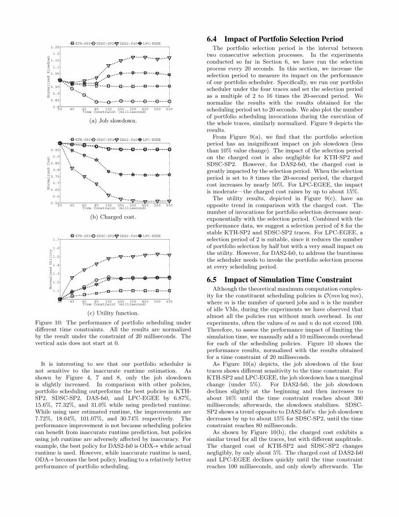
Figure 10: The performance of portfolio scheduling underdifferent time constraints. All the results are normalizedby the result under the constraint of 20 milliseconds. Thevertical axis does not start at 0.

It is interesting to see that our portfolio scheduler isnot sensitive to the inaccurate runtime estimation. Asshown by Figure 4, 7 and 8, only the job slowdownis slightly increased. In comparison with other policies,portfolio scheduling outperforms the best policies in KTH-SP2, SDSC-SP2, DAS-fs0, and LPC-EGEE by 6.87%,15.6%, 77.32%, and 31.0% while using predicted runtime.While using user estimated runtime, the improvements are7.72%, 18.04%, 101.07%, and 30.74% respectively. Theperformance improvement is not because scheduling policiescan benefit from inaccurate runtime prediction, but policiesusing job runtime are adversely affected by inaccuracy. Forexample, the best policy for DAS2-fs0 is ODX-∗ while actualruntime is used. However, while inaccurate runtime is used,ODA-∗ becomes the best policy, leading to a relatively betterperformance of portfolio scheduling.

6.4 Impact of Portfolio Selection PeriodThe portfolio selection period is the interval between

two consecutive selection processes. In the experimentsconducted so far in Section 6, we have run the selectionprocess every 20 seconds. In this section, we increase theselection period to measure its impact on the performanceof our portfolio scheduler. Specifically, we run our portfolioscheduler under the four traces and set the selection periodas a multiple of 2 to 16 times the 20-second period. Wenormalize the results with the results obtained for thescheduling period set to 20 seconds. We also plot the numberof portfolio scheduling invocations during the execution ofthe whole traces, similarly normalized. Figure 9 depicts theresults.

From Figure 9(a), we find that the portfolio selectionperiod has an insignificant impact on job slowdown (lessthan 10% value change). The impact of the selection periodon the charged cost is also negligible for KTH-SP2 andSDSC-SP2. However, for DAS2-fs0, the charged cost isgreatly impacted by the selection period. When the selectionperiod is set to 8 times the 20-second period, the chargedcost increases by nearly 50%. For LPC-EGEE, the impactis moderate—the charged cost raises by up to about 15%.

The utility results, depicted in Figure 9(c), have anopposite trend in comparison with the charged cost. Thenumber of invocations for portfolio selection decreases near-exponentially with the selection period. Combined with theperformance data, we suggest a selection period of 8 for thestable KTH-SP2 and SDSC-SP2 traces. For LPC-EGEE, aselection period of 2 is suitable, since it reduces the numberof portfolio selection by half but with a very small impact onthe utility. However, for DAS2-fs0, to address the burstinessthe scheduler needs to invoke the portfolio selection processat every scheduling period.

6.5 Impact of Simulation Time ConstraintAlthough the theoretical maximum computation complex-

ity for the constituent scheduling policies is O(mn logmn),where m is the number of queued jobs and n is the numberof idle VMs, during the experiments we have observed thatalmost all the policies run without much overhead. In ourexperiments, often the values of m and n do not exceed 100.Therefore, to assess the performance impact of limiting thesimulation time, we manually add a 10 milliseconds overheadfor each of the scheduling policies. Figure 10 shows theperformance results, normalized with the results obtainedfor a time constraint of 20 milliseconds.

As Figure 10(a) depicts, the job slowdown of the fourtraces shows different sensitivity to the time constraint. ForKTH-SP2 and LPC-EGEE, the job slowdown has a marginalchange (under 5%). For DAS2-fs0, the job slowdowndeclines slightly at the beginning and then increases toabout 16% until the time constraint reaches about 300milliseconds; afterwards, the slowdown stabilizes. SDSC-SP2 shows a trend opposite to DAS2-fs0’s: the job slowdowndecreases by up to about 15% for SDSC-SP2, until the timeconstraint reaches 80 milliseconds.

As shown by Figure 10(b), the charged cost exhibits asimilar trend for all the traces, but with different amplitude.The charged cost of KTH-SP2 and SDSC-SP2 changesnegligibly, by only about 5%. The charged cost of DAS2-fs0and LPC-EGEE declines quickly until the time constraintreaches 100 milliseconds, and only slowly afterwards. The

charged cost is reduced by 20% and 40%, respectively.The utility obtained for each trace exhibits similar trends

when the simulation time constraint increases. The utility ofall the traces increases until the time constraint reaches 200milliseconds, then changes only slightly afterwards. Becausea policy requires 10 milliseconds for simulation, the totalnumber of simulated policies is 20. Therefore, for ourportfolio scheduler, simulating a third of the total amount ofpolicies (60) is sufficient. The reason can be found if we lookback at Figure 5(b). As we pick 60% of the simulated policiesas Smart policies, the number of policies in the Smart setwould be 12. This covers almost all the dominant policiesin Figure 5(b), which indicates the effectiveness of our time-constrained simulation algorithm.

7. RELATED WORKIn this section, we provide a review on research work

related to three areas: computational portfolio design andportfolio-based algorithm selection, parallel job scheduling,and scientific workload scheduling in the cloud.In 1976, Rice introduced the algorithm selection problem:

with so many available algorithms, which one should beselected to solve the specific problem instance in orderto optimize some performance objective [29]. Meanwhile,Rice presented an abstract model that can be used toexplore the problem [29, 34]. However, the most widely-adopted solution to the problem follows a ”winner-take-all” approach which selects the algorithm that has the bestaverage performance for all performance instances [45]. In1997, Huberman [12] introduced an economics approachbased on portfolio theory [24] to the problem and proposeda general procedure for computational portfolio design. Theidea is that by combining many algorithms into portfolios,a whole range of problem instances can be addressed. Ourprevious work [8] adapted the seminar idea and proposeda portfolio scheduler for scheduling scientific workloadsin the data center; in parallel with our work but for adifferent setting, Shai et al. have looked at a type ofportfolio scheduling without auto-tuning [30]. The focusof previous work is to answer the question how to useportfolio scheduling and if it works. In this article, we applyRice’s abstract model to portfolio scheduling and present ascheduler framework based the model for a more general anddemanding application model. We explore the functionalityof our scheduler and focus on the question: given dozens ofpolicies, how to reduce the overhead of portfolio scheduling.A large body of research work has been done on job

scheduling in parallel computer systems. First-Come-First-Serve (FCFS) [18] is the earliest and simplest schedulingpolicy widely used in production batch systems. To reducethe fragmentation caused by head-of-line blocking in FCFSscheduling [3], EASY-Backfilling was introduced [20]. Afterthat, many variants were designed to improve EASY-Backfilling [5, 19, 32, 37, 38, 44]. Among them, the adaptivescheduling policies are most relevant to our work [5, 19, 38]:they use different policies in different periods of time forscheduling; they also use online simulation to select the bestpolicy for the next scheduling period. However, they arefundamentally different from our work. Firstly, they choosethe policy that performs best for the previous workload,while our work chooses the best policy based on currentworkload. Secondly, instead of presenting a specificalscheduler, we proposed an abstract model and a framework

for portfolio scheduling, which can be easily adapted to otherscheduling areas. Last but not least, the major focus ofour work is to explore portfolio scheduling itself and to findmethods to reduce the overhead of scheduling in case thenumber of constituent policies are enormous.

The construction of our policy portfolio relies on previousstudies related to utility-based job scheduling and scientificworkload scheduling in the cloud. Similarly to our previouswork [41], we divide the scheduling policy into three parts:resource provisioning, job selection, and VM selection.For the first part, we surveyed recent study on resourceprovisioning and allocation in the cloud, and selected thepolicies that both perform well and are suitable for paralleljob scheduling for the construction of policy portfolio [8,10, 25, 27, 41, 43]. The selected policies are also limited toidentical type of on-demand VMs, and we refer to our priorwork [31] for policies using multiple instance types. Forjob selection policies, we selected four utility functions fromTang’s work [39] which covers most of the priority functionsused in the literature. We don’t consider backfilling inour current scheduling policies. We leave it for the futurework and refer to [7] for its preliminary result on schedulingparallel jobs in the cloud. For VM selection policies, weselected three heuristics for the problem of bin packing [6].We have briefly described the policies in Section 3.1 andmore details can be found in the original work.

8. CONCLUSION AND FUTURE WORKThe elasticity of cloud computing and data center com-

puting has shown great potential for scientific computing.In this article, we investigated the long-term execution ofparallel scientific workloads on IaaS cloud resources. Insteadof finding more sophisticated scheduling algorithms, we haveproposed the use of portfolio scheduling, which combinesmany existing policies into a portfolio and selects online anappropriate policy to match specific workload and systemconditions. We have first introduced an abstract modelfor the exploration of portfolio scheduling. Based on thismodel, we have designed a portfolio scheduling frameworkthat includes several performance-affecting configurationparameters. Our framework combines over 60 policies—resource provisioning, job allocation, and VM allocation—into a single comprehensive portfolio. We have designeda versatile utility function and implemented an onlinesimulator to select the right policy for the given workload.To address the critical issue of selecting an appropriatepolicy in time, we have proposed an algorithm for time-constrained policy selection, which aims at increasing thechance of selecting the best policy even under time limitsthat prevent the exhaustive evaluation of policies.

We have evaluated the performance of our portfolioscheduler through simulations, using four long-term real-world traces collected from parallel production environ-ments. We have explored the impact on performanceof different portfolio configurations, of inaccurate runtimeprediction, and of different time constraints on policyselection. We found that (1) by exploiting the collectivestrengths of the constituent policies, our portfolio scheduleroutperforms its best constituent policy; (2) although thecharged cost for the traces used in our experiment is hardlyreduced, as the system utilization is relatively high, it isstill worthwhile to improve user-impacting performance suchas the job slowdown; (3) while policies using job runtime

are badly affected by inaccurate information, our portfolioscheduler is much less sensitive; (4) for bursty workloads, theportfolio scheduler must make frequent decisions to achievegood performance; for stable workloads, long intervalsbetween decisions suffice; (5) by clustering the policies intodifferent categories, our simulation algorithm can reach goodperformance despite simulating only a few of the policies.For the future, we want to find out whether and to what

extend the reflection can help improve the quality of theselected policies. Secondly, we plan to develop an algorithmthat can dynamically trigger the portfolio simulation processonly when the workload pattern changes, thus reducing thenumber of invocations while preserving the performance.Thirdly, we intend to implement a real-world prototype ofthe scheduler and conduct realistic experiments to studyperformance of portfolio scheduling in practice. Finally,we are adapting portfolio scheduling for the execution ofscientific workflows and expect that more application typescan benefit from this new scheduling solution.

AcknowledgmentThe authors would like to thank all the reviewers fortheir comments and positive feedbacks on our paper. Thiswork is partially funded by the Dutch national researchprogram COMMIT; and supported by the STW/NWO Venigrant 11881, the National Natural Science Foundation ofChina (Grant No. 60903042 and 61272483), and the R&DSpecial Fund for Public Welfare Industry (Meteorology)GYHY201306003.

9. REFERENCES[1] Parallel workloads archive.

http://www.cs.huji.ac.il/labs/parallel/workload/.2013-02-17.

[2] O. Agmon Ben-Yehuda, A. Schuster, A. Sharov,M. Silberstein, and A. Iosup. Expert: Pareto-efficienttask replication on grids and a cloud. In IPDPS, pages167–178, 2012.

[3] A. AuYoung, A. Vahdat, and A. C. Snoeren.Evaluating the impact of inaccurate information inutility-based scheduling. In SC, 2009.

[4] R. N. Calheiros, R. Ranjan, A. Beloglazov, C. A.F. D. Rose, and R. Buyya. Cloudsim: a toolkit formodeling and simulation of cloud computingenvironments and evaluation of resource provisioningalgorithms. Softw., Pract. Exper., 41(1):23–50, 2011.

[5] S.-H. Chiang and S. Vasupongayya. Design andpotential performance of goal-oriented job schedulingpolicies for parallel computer workloads. IEEE Trans.Parallel Distrib. Syst., 19(12):1642–1656, 2008.

[6] E. G. Coffman, Jr., M. R. Garey, and D. S. Johnson.Approximation algorithms for bin packing: a survey.In Approximation algorithms for NP-hard problems,pages 46–93. PWS Publishing Co., Boston, MA, USA,1997.

[7] M. D. de Assuncao, A. di Costanzo, and R. Buyya.Evaluating the cost-benefit of using cloud computingto extend the capacity of clusters. In HPDC, pages141–150, 2009.

[8] K. Deng, R. Verboon, K. Ren, and A. Iosup. Aperiodic portfolio scheduler for scientific computing inthe data center. In JSSPP, 2013, To Appear.

[9] D. G. Feitelson, L. Rudolph, and U. Schwiegelshohn.Parallel job scheduling - a status report. In JSSPP,pages 1–16, 2004.

[10] S. Genaud and J. Gossa. Cost-wait trade-offs inclient-side resource provisioning with elastic clouds. InIEEE CLOUD, pages 1–8, 2011.

[11] T. J. Hacker and K. Mahadik. Flexible resourceallocation for reliable virtual cluster computingsystems. In SC, page 48, 2011.

[12] B. A. Huberman, R. M. Lukose, and T. Hogg. Aneconomics approach to hard computational problems.Science, 275(5296):51–54, 1997.

[13] A. Iosup, S. Ostermann, N. Yigitbasi, R. Prodan,T. Fahringer, and D. H. J. Epema. Performanceanalysis of cloud computing services for many-tasksscientific computing. IEEE Trans. Parallel Distrib.Syst., 22(6):931–945, 2011.

[14] A. Iosup, O. O. Sonmez, S. Anoep, and D. H. J.Epema. The performance of bags-of-tasks inlarge-scale distributed systems. In HPDC, pages97–108, 2008.

[15] A. Iosup, O. O. Sonmez, and D. H. J. Epema. Dgsim:Comparing grid resource management architecturesthrough trace-based simulation. In Euro-Par, pages13–25, 2008.

[16] K. Keahey, R. Figueiredo, J. Fortes, T. Freeman, andM. Tsugawa. Science clouds: Early experiences incloud computing for scientific applications. Cloudcomputing and applications, 2008:16, 2008.

[17] K. Keahey and T. Freeman. Contextualization:Providing one-click virtual clusters. In eScience, pages301–308, 2008.

[18] P. Krueger, T.-H. Lai, and V. A. Dixit-Radiya. Jobscheduling is more important than processorallocation for hypercube computers. IEEE Trans.Parallel Distrib. Syst., 5(5):488–497, 1994.

[19] B. Lawson and E. Smirni. Self-adaptive schedulerparameterization via online simulation. In IPDPS,2005.

[20] D. A. Lifka. The anl/ibm sp scheduling system. InJSSPP, pages 295–303, 1995.

[21] M. Malawski, G. Juve, E. Deelman, and J. Nabrzyski.Cost- and deadline-constrained provisioning forscientific workflow ensembles in iaas clouds. In SC,page 22, 2012.

[22] M. Mao and M. Humphrey. Auto-scaling to minimizecost and meet application deadlines in cloudworkflows. In SC, page 49, 2011.

[23] M. Mao and M. Humphrey. A performance study onthe vm startup time in the cloud. In IEEE CLOUD,pages 423–430, 2012.

[24] H. Markowitz. Portfolio selection*. The journal offinance, 7(1):77–91, 1952.

[25] P. Marshall, H. M. Tufo, and K. Keahey. Provisioningpolicies for elastic computing environments. In IPDPSWorkshops, pages 1085–1094, 2012.

[26] A. M. Matsunaga and J. A. B. Fortes. On the use ofmachine learning to predict the time and resourcesconsumed by applications. In CCGRID, pages495–504, 2010.

[27] E. Michon, J. Gossa, and S. Genaud. Free elasticity

and free cpu power for scientific workloads on iaasclouds. In ICPADS, pages 85–92, 2012.

[28] A.-M. Oprescu, T. Kielmann, and H. Leahu.Stochastic tail-phase optimization for bag-of-tasksexecution in clouds. In UCC, pages 204–208, 2012.

[29] J. R. Rice. The algorithm selection problem. Advancesin Computers, 15:65–118, 1976.

[30] O. Shai, E. Shmueli, and D. G. Feitelson. Heuristicsfor resource matching in intel’s compute farm. InJSSPP, 2013, To Appear.

[31] S. Shen, K. Deng, A. Iosup, and D. H. J. Epema.Scheduling jobs in the cloud using on-demand andreserved instances. In Euro-Par, pages 242–254, 2013.

[32] E. Shmueli and D. G. Feitelson. Backfilling withlookahead to optimize the packing of parallel jobs. J.Parallel Distrib. Comput., 65(9):1090–1107, 2005.

[33] W. Smith. Prediction services for distributedcomputing. In IPDPS, pages 1–10, 2007.

[34] K. Smith-Miles. Cross-disciplinary perspectives onmeta-learning for algorithm selection. ACM Comput.Surv., 41(1), 2008.

[35] O. O. Sonmez, N. Yigitbasi, S. Abrishami, A. Iosup,and D. H. J. Epema. Performance analysis of dynamicworkflow scheduling in multicluster grids. In HPDC,pages 49–60, 2010.

[36] O. O. Sonmez, N. Yigitbasi, A. Iosup, and D. H. J.Epema. Trace-based evaluation of job runtime andqueue wait time predictions in grids. In HPDC, pages111–120, 2009.

[37] S. Srinivasan, R. Kettimuthu, V. Subramani, andP. Sadayappan. Selective reservation strategies forbackfill job scheduling. In JSSPP, pages 55–71, 2002.

[38] D. Talby and D. G. Feitelson. Improving andstabilizing parallel computer performance usingadaptive backfilling. In IPDPS, 2005.

[39] W. Tang, Z. Lan, N. Desai, and D. Buettner.Fault-aware, utility-based job scheduling on blue,gene/p systems. In CLUSTER, pages 1–10, 2009.

[40] D. Tsafrir, Y. Etsion, and D. G. Feitelson. Backfillingusing system-generated predictions rather than userruntime estimates. IEEE Trans. Parallel Distrib.Syst., 18(6):789–803, 2007.

[41] D. Villegas, A. Antoniou, S. M. Sadjadi, and A. Iosup.An analysis of provisioning and allocation policies forinfrastructure-as-a-service clouds. In CCGRID, pages612–619, 2012.

[42] G. von Laszewski, J. Diaz, F. Wang, and G. Fox.Comparison of multiple cloud frameworks. In IEEECLOUD, pages 734–741, 2012.

[43] L. Wang, J. Zhan, W. Shi, and Y. Liang. In cloud, canscientific communities benefit from the economies ofscale? IEEE Trans. Parallel Distrib. Syst.,23(2):296–303, 2012.

[44] A. M. Weil and D. G. Feitelson. Utilization,predictability, workloads, and user runtime estimatesin scheduling the ibm sp2 with backfilling. IEEETrans. Parallel Distrib. Syst., 12(6):529–543, 2001.

[45] L. Xu, F. Hutter, H. H. Hoos, and K. Leyton-Brown.Satzilla: Portfolio-based algorithm selection for sat. J.Artif. Intell. Res. (JAIR), 32:565–606, 2008.

exploring portfolio scheduling for long-term execution of scientific

Documents