exploring the effects of yard management and neighborhood
TRANSCRIPT
Exploring the Effects of
Yard Management and Neighborhood Influence
on Carbon Storage in Residential Subdivisions
An Agent-Based Modeling Approach
Meghan D. Hutchins
A thesis submitted in partial fulfillment of the requirements
for the degree ofMaster of Science
(Natural Resources and the Environment)University of Michigan
2010
Thesis Committee:
Associate Professor William S. Currie, Chair Professor Joan Iverson NassauerAssociate Professor Rick L. Riolo

AbstractThe dramatic land-use shift from forest and agricultural to exurban residential land uses creates an
excellent opportunity for ecosystem restoration and carbon sequestration through yard design and
management. Yard management in a residential subdivision is rarely an autonomous endeavor. Cultural
and local norms play an important role in how residents design and maintain their yards. Studies show
that residents are influenced by the behavior of their neighbors. Yet, social influence has rarely been
incorporated into carbon sequestration studies in residential landscapes. Agent-based modeling offers
an ideal framework for exploring how social complexities among humans could affect their
environment.
An agent-based model called ELMST (Exploratory Land Management and Carbon Storage), was
developed to explore how management of individual yards and neighborhood influence could affect
carbon storage at the scale of a residential subdivision. The model was run under four scenarios: (tier-0)
no management, (tier-1) individual management without influence (tier-2) individual management with
opportunity to adapt based on neighbor behaviors, and (tier-3) adaptive management, as in tier-2, but
several residents were given an incentive to innovate their yard to a native prairie design upon model
start-up. The model was parameterized with interview and fieldwork data from exurban homes
Southeast Michigan. Total carbon within the subdivision was compared among scenarios for year 30.
Tier-1 showed a significantly higher quantity of carbon than all others, including tier-0 (no
management). Results from tier-2 and tier-3 showed a greater variability of carbon storage at the
subdivision level, suggesting that a wide range of outcomes can emerge as a result of neighborhood
influence and divergent local norms. Considering model sensitivity of individual management
behaviors, the model showed that turfgrass fertilization and mowing the lawn while allowing grass
clippings to decompose on-site dramatically increased carbon stored at the parcel level, when compared
with the no management scenario. Comparatively, removing grass clippings dramatically decreased
carbon stored at the parcel level, when compared with the no management scenario. The native prairie
innovation was able to propagate through the subdivision in tier-3 in the ELMST model. Prairie-based
parcels were shown to store less carbon overall than the conventional lawn-based parcels that were
fertilized or mown while allowing grass clippings to remain on-site, but stored more carbon than if
grass clippings were removed all together. Model results imply that trade-off between carbon storage
ii

and other ecosystem services may need to be considered when developing policies for
environmentally-friendly residential landscapes.
The ELMST model was developed to be expanded and re-used for a variety of locales, cultures and
climates. Results from this study may be used to formulate better research questions and hypothesis,
inform data collection, expand intuition of policy makers, and advance the development of agent-based
models with regards to coupled human and natural systems.
iii

Acknowledgements
I would like to thank my committee members, Bill Currie, Joan Nassauer and Rick Riolo for all their
time, patience and guidance. Thank you to Derek Robinson for being a superb mentor and Dan Brown
for being an excellent motivator. Many thanks to the entire Project Sluce2 team. Without their
comprehensive knowledge and support, this thesis would not be possible; to Brendan Carson and
Lauren Lesch, for making the 2009 Summer fieldwork and interviews both fun and memorable. Thank
you to Joyce Lee and Jack Iwashyna who sparked my interest in social influence, network modeling
and who gave me a jump start on developing agent-based models with Repast Simphony. A special
thanks to Chad Hanson and Evan Fletcher for their kind help with words and scripts respectively, and
to Peter Gamberg for his encouragement and providing weekly “sanity” trips to Frank's Diner. Lastly,
thank you to my friends and family for all their support and enthusiasm.
iv
ContentsAbstract.....................................................................................................................................................iiAcknowledgements.................................................................................................................................ivIntroduction..............................................................................................................................................1
Background...........................................................................................................................................2Carbon Storage.................................................................................................................................3Default Management........................................................................................................................4Neighborhood Influence...................................................................................................................5Agent-Based Models........................................................................................................................8
Summary...............................................................................................................................................9Research Questions and Hypothesis.....................................................................................................10Methods ..................................................................................................................................................12
Model Description...............................................................................................................................13Overview.........................................................................................................................................13Design Concepts.............................................................................................................................18Details.............................................................................................................................................21
Statistical Analysis..............................................................................................................................29Results.....................................................................................................................................................29
Model Verification and Validation.......................................................................................................29Effect of Individual Management Behaviors......................................................................................32Model Application ..............................................................................................................................32
Tier-0 – No Management ...............................................................................................................32Tier-1 – Intrinsic Management ......................................................................................................33Tier-2 – Adaptive Management .....................................................................................................33Tier-3 – Adaptive Management with Incentive to Innovate...........................................................33Hypothesis Results: Comparison Among Tiers..............................................................................34
Discussion................................................................................................................................................34Effect of Individual Management Behaviors......................................................................................34Research Question 1: Intrinsic Management and Carbon Storage......................................................34Research Question 2: Adaptive Management and Carbon Storage.....................................................36Research Question 3: Adaptive Management with Incentive to Innovate..........................................37Further Research..................................................................................................................................38
Conclusion...............................................................................................................................................39Figures.....................................................................................................................................................40Tables.......................................................................................................................................................49References...............................................................................................................................................58Appendix I: Visualizations of Select ELMST Model Runs................................................................63
v
FiguresFigure 1: Tier-Based Research Schematic...............................................................................................40Figure 2: Conceptual Model Overview....................................................................................................41Figure 3: Subdivision Environment and Social Network Structure.........................................................41Figure 4: Ecosystem Components............................................................................................................42Figure 5: Unmanaged Carbon-Cycle.......................................................................................................42Figure 6: Managed Carbon-Cycle............................................................................................................43Figure 7: Seasonal Processes and Agent Activities..................................................................................44Figure 8: ELMST Class Diagram............................................................................................................45Figure 9: Effect of Individual Management Behaviors on Total Subdivision Carbon.............................46Figure 10: Model Results: Histograms of Total Average Subdivision Carbon by Tier............................47Figure 11: Model Results: Box Plot of Total Average Subdivision Carbon by Tier................................48Figure 12: Validation: Unmanaged Turf Grass Carbon Pools – 200 Years..............................................63Figure 13: Validation: Unmanaged Turf Grass Carbon Pools – 20 Years................................................63Figure 14: Validation: Unmanaged Tree Cover Carbon Pools – 100 Years.............................................64Figure 15: Validation: Unmanaged Tree Cover Litter Pools – 100 Years................................................64Figure 16: Validation: Unmanaged Prairie Carbon Pools – 1000 Years..................................................65Figure 17: Validation: Unmanaged Prairie Carbon Pools – 20 Years......................................................65Figure 18: Tier-0 Sample Run: Turfgrass Carbon Pools – 50 Years........................................................66Figure 19: Tier-0 Sample Run: Tree Cover Carbon Pools – 50 Years.....................................................66Figure 20: Tier-0 Sample Run: Prairie Carbon Pools – 50 Years.............................................................67Figure 21: Tier-0 Sample Run: Total Subdivision By Carbon Pool – 50 Years.......................................68Figure 22: Tier-0 Sample Run: Total Subdivision Carbon By Land-Cover Type – 50 Years..................68Figure 23: Tier-0 Sample Run: Total Subdivision Carbon – 50 Years.....................................................69Figure 24: Tier-1 Sample Run: Proportion of Resident Behaviors – 30 Years........................................70Figure 25: Tier-1 Sample Run: Proportion of Lawn Mowing Schedules – 30 Years...............................70Figure 26: Tier-1 Sample Run: Turfgrass Carbon Pools – 50 Years........................................................71Figure 27: Tier-1 Sample Run: Tree Cover Carbon Pools – 50 Years.....................................................71Figure 28: Tier-1 Sample Run: Prairie Carbon Pools – 50 Years.............................................................72Figure 29: Tier-1 Sample Run: Total Subdivision By Carbon Pool – 50 Years.......................................73Figure 30: Tier-1 Sample Run: Total Subdivision Carbon by Land-Cover Type – 50 Years...................73Figure 31: Tier-1 Sample Run: Total Subdivision Carbon – 50 Years.....................................................74Figure 32: Tier-2 Sample Run: Proportion of Resident Behaviors – 30 Years........................................75Figure 33: Tier-2 Sample Run: Proportion of Lawn Mowing Schedules – 30 Years...............................75Figure 34: Tier-2 Sample Run: Turfgrass Carbon Pools – 50 Years........................................................76Figure 35: Tier-2 Sample Run: Tree Cover Carbon Pools – 50 Years.....................................................76Figure 36: Tier-1 Sample Run: Prairie Carbon Pools – 50 Years.............................................................77Figure 37: Tier-2 Sample Run: Total Subdivision Carbon by Carbon Pool – 50 Years...........................78Figure 38: Tier-2 Sample Run: Total Subdivision Carbon by Land-Cover Type – 50 Years...................78Figure 39: Tier-2 Sample Run: Total Subdivision Carbon – 50 Years.....................................................79Figure 40: Tier-3 Sample Run: Proportion of Resident Behaviors – 30 Years........................................80Figure 41: Tier-3 Sample Run: Proportion of Lawn Mowing Schedules – 30 Years...............................80Figure 42: Tier-3 Sample Run: Turfgrass Carbon Pools – 50 Years........................................................81Figure 43: Tier-3 Sample Run: Tree Cover Carbon Pools – 50 Years.....................................................81Figure 44: Tier-3 Sample Run: Prairie Carbon Pools – 50 Years.............................................................82
vi
Figure 45: Tier-3 Sample Run: Total Subdivision Carbon by Carbon Pool – 50 Years...........................83Figure 46: Tier-3 Sample Run: Total Subdivision Carbon by Land-Cover Type – 50 Years...................83Figure 47: Tier-3 Sample Run: Total Subdivision Carbon – 50 Years.....................................................84
TablesTable 1: Ecosystem Initialization Parameters.........................................................................................49Table 2: Resident Initialization Parameters..............................................................................................50Table 3: Validation of Unmanaged ELMST Carbon Density..................................................................51Table 4: Verification of Resident Behavior Across Research Tiers.........................................................52Table 5: Sensitivity of Management Behaviors on Total Subdivision Carbon........................................53Table 6: Model Component Activation Across Research Tier Scenarios................................................53Table 7: Model Results: Average Parcel Land-Cover Area Across Research Tiers.................................54Table 8: Model Results: Average Carbon Density Across Research Tiers...............................................54Table 9: Model Results: Total Average Subdivision Carbon Across Tiers...............................................55Table 10: Hypothesis Results for Total Subdivision Carbon Over Year 30.............................................56Table 11: Fieldwork: Eco-Zone Categories Translated to ELMST Land-Cover Types...........................57Table 12: Fieldwork: Land-Cover Areas for Parcels of One Acre or Less..............................................57
vii
1
Introduction
Climate change due to carbon dioxide and other greenhouse gas accumulations in the atmosphere is a
global issue. Between 1850 and 1998, approximately 405 Gt of carbon dioxide was emitted into the
atmosphere, increasing the concentration of carbon from 285 ppmv to 366 ppmv (approximately 28
percent) through the burning of fossil fuels, cement production, and land-use/land-cover change (IPCC
2000). While a portion of these anthropogenic emissions are absorbed by oceans and terrestrial
ecosystems, at least 40 percent remain in the atmosphere (IPCC 2000).
Addressing the excess atmospheric carbon is an increasing topic of interest. Terrestrial sequestration
may be included in a suite of possible solutions to remove excess carbon from the atmosphere. Many
programs have been created to explicitly enhance terrestrial carbon sequestration through reforestation
programs and agricultural land management practices (Benson & Surles 2006). Policies may take time
to implement and could incur unexpected costs and limitations. This thesis investigates a relatively
low-cost and convenient means of carbon sequestration through simple yard management practices in
residential subdivisions. In 2000, residential areas accounted for 13.4 percent of the conterminous
United States and were expanding at a rate of 1.60 percent per year – out-pacing the rate of population
growth by roughly 25 percent (Theobald 2005). The distributed land management practices inherent
across residential landscapes may offer an opportunity for climate change mitigation through terrestrial
carbon storage and other ecosystem services.
Cultural and local norms play an important role in how residents design and maintain their yards.
Studies show that residents are influenced by what their neighbors do (Galster 1987; Nassauer, Wang,
& Dayrell 2009; Ioannides 2002). However, a current gap in scientific knowledge relates to how
neighborhood influence could affect adoption of management regimes and yard types at the parcel
level, which are likely to have implications for carbon storage at the subdivision level. An agent-based
model, ELMST (Exploratory Land Management and Carbon Storage) was created to compare four yard
management scenarios in terms of potential carbon storage at the subdivision level. The model offers
an exploration into how social influence among residential neighbors may affect human-ecosystem
interactions within individual parcels. The ELMST model operates at the parcel-level, however,
measurements are addressed at the subdivision level to show how individual behaviors scale-up to
create landscape-level phenomena.
2
The overarching research question is "how could resident management and neighborhood influence
affect carbon storage in the vegetation and soils of a residential subdivision?" The scenarios presented
in this study are tier-based: (tier-0) no management, (tier-1) individual management without influence
(tier-2) individual management with opportunity to adapt based on neighbor behaviors, and (tier-3)
adaptive management, as in tier-2, but several residents were given an incentive to innovate their yard
to a native prairie design upon model start-up. Empirical data from homeowner interviews and
fieldwork in exurban residential areas of Southeast Michigan were used to parameterize the model
whenever possible, otherwise reasonable values from literature were used. As a result, this study is
particular to the vegetation, climate and culture of Southeast Michigan exurban residential areas.
This thesis offers a unique contribution to the studies of climate change science, land-use/land-cover
change (LUCC), and coupled human and natural systems (CHANS) in that it addresses the social
aspects of land management and resulting effects on carbon storage and sequestration. A contribution to
the area of complex systems and agent-based modeling is also provided through the development of
ELMST, a novel agent-based model created to be re-used for a variety of locales, cultures and climates.
Background
More than three-quarters of the Earth’s ice-free land has been altered by humans (Ellis & Ramankutty
2008). Human activities alter the natural carbon stocks and fluxes in terrestrial carbon pools through
land-use change, land-cover change and land management. Land-use and land-cover change (LUCC)
account for more than 30% of the carbon efflux into the atmosphere – a rate exceeded only by the
burning of fossil fuels (Dixon et al. 1994; IPCC 2000). Land-use alterations are largely due to
conversion from forests and prairies to farm fields and other agricultural lands (Houghton, Hackler, &
Lawrence 1999). Alterations have serious implications on plant and animal communities, soil
composition, water quality, and many other ecosystem services (Wu 2002).
The United States has seen dramatic LUCC shifts since 1950 – the most dramatic being the expansion
of exurban areas just beyond the urban-rural fringe1. A study conducted by Brown et al. (2005) found
that between 1950 and 2000, the area of urban land-use increased by one percent while cropland
1 An on-line animation of eastern U.S. patterns of urban, suburban, exurban and rural development from 1980 to 2020: http://www.ecologyandsociety.org/include/getdoc.php?articleid=1390&type=figure11 (Theobald 2005)
3
decreased by 11 percent. The decrease in agricultural land was primarily due to the development of
exurban land uses, which increased sevenfold to tenfold during this same time period (Brown et al.
2005).
Carbon Storage
Agricultural fields are commonly stripped of vegetation, soil organic carbon and other nutrients as a
result of intensive row-crop agriculture (Meyer, Baer, & Whiles 2008; Pouyat, Yesilonis, &
Golubiewski 2008). The dramatic land-use shift from agricultural to exurban residential land creates an
excellent opportunity for ecosystem restoration and carbon sequestration (Brown et al. 2005; Lesch
2010). Developers will typically purchase an agricultural field from a farmer for residential subdivision
development. The soil will be graded, homes will be built, and turfgrass will be established. In some
cases, small trees may also be planted (Westbrook 2010). When a resident moves into their new home,
decisions will be made regarding how to best manage the vegetation in the yard. Management activities
include tasks such as mowing the lawn, removing fallen leaves, and yard re-design. Because
neighborhood yards are relatively discrete and thought to be managed autonomously by their owners,
the carbon dynamics in one parcel may be significantly different from the carbon dynamics in another
parcel. The mosaic of individual yard designs and management regimes at the parcel-level are likely to
have macro-level impacts at the subdivision level (Kaye et al. 2006). Through distributed land
management, residential subdivisions have the potential to be a cost-effective venue for carbon
sequestration – especially given the large and expanding areas of exurban development (Brown et al.
2005; Theobald 2005; Bowman & Thompson 2009).
In terrestrial ecosystems, atmospheric carbon is sequestered through the process of photosynthetic
growth and stored as biomass in living vegetation, such as grasses and trees. Vegetation will naturally
senesce to produce litter which will decompose over time. Decomposition allows a portion of litter
carbon (about 20 percent) to be transfered to the soil; the remainder is respired back to the atmosphere
in the form of carbon dioxide (Currie & Aber 1997). Carbon stored in soil may respire back to the
atmosphere, however soil respiration occurs at a considerably lower rate when compared with litter
decomposition (Kucharik et al. 2001). The amount of time carbon spends in each pool (living biomass,
litter and soil) is defined as the mean residence time. Mean residence time (MRT) plays a crucial role in
the carbon cycle. Grasses, leaves and litter have an MRT of months to years, while woody biomass and
4
soils have an MRT of years, decades or even centuries, making these pools relatively persistent stocks
of carbon (IPCC 2000).
Humans participate in the carbon cycle through LUCC and management activities. Neighborhood
residents manage the vegetation in their yards, thereby changing the MRT within a given carbon pool.
For example, if a resident decides to remove fallen leaves from her yard, carbon is not only removed
from the litter pool, but is also denied transfer to the soil pool. When a resident mows her lawn and
allows grass clippings to remain on the turfgrass, additional carbon is transferred to the litter pool, and
eventually to the soil pool through decomposition. The processes of photosynthetic growth,
decomposition and respiration play important roles in net flux of carbon between vegetation, litter, soil
and atmosphere. Human-induced management activities may affect the natural carbon flux, thereby
changing the way a landscape stores and sequesters carbon (IPCC 2000).
Default Management
Developers play an important role in pioneer resident management practices and local norms. For
example, developers understand the importance of turfgrass areas for active families (Westbrook 2010),
implying that active families purchase yards with large areas of turfgrass and will manage the turfgrass
accordingly. Similarly, developers who create innovative subdivisions with open spaces and
conservation features will market these neighborhoods to a particular audience in order to receive the
best price (Bowman & Thompson 2009). Initial landscapes not only attract a particular audience, they
also suggest aesthetic cues to care (Nassauer 1993), which may have profound effects on future local
norms in the subdivision.
Developers invest significant time and resources when developing a new subdivision, and these
investments come without a guaranteed payoff (Bowman & Thompson 2009). Risks associated with
subdivision design, planning and engineering lead developers to create conventional subdivisions that
have historically been known to meet revenue goals (Westbrook 2010; Bowman & Thompson 2009).
According to research conducted by Westbrook (2010), developers acknowledge a value in ecological
design alternatives, such as low-impact development or conservation design (Bowman & Thompson
2009). However, these techniques require changes to standard planning and engineering, and have not

5
been consumer tested in specific areas. Changes to standard development and uncertain marketability
increase the risk of innovative, ecological designs even further. Home-buyers are also at financial risk
when purchasing innovative property, anticipating uncertainty of re-sale and estimated property value.
Thaler and Sunstein describe the concept of "choice architects" in their 2009 book, Nudge. Choice
architects organize the context of human decision-making and behavior by creating a "default" designs.
The book argues that behavior is predictably altered by default circumstances, and that there is "no
such thing as a 'neutral' design" (Thaler & Sunstein 2009, p. 3). Developers may unknowingly be
choice architects whose development strategies are likely to effect how future residents will manage
their yards. Initial yard design may have a significant impact on local subdivision norms and ultimately
carbon storage patterns over time.
The potential to leverage ecologically friendly outcomes through default yard designs is not often
practiced – the perceived financial risk may be too great and consumers may be reluctant to buy in.
While this paper acknowledges the importance of developers as choice architects with respect to initial
yard design and ecosystem services, the depth of this topic is beyond the scope of this thesis. The focus
of this paper is placed on conventional subdivisions; subdivisions that developers create with the
perceived confidence of meeting revenue goals.
Neighborhood Influence
In 1997, a National Housing Survey conducted by Fannie Mae found that 71 percent of Americans
preferred a "single-family detached house with a yard on all sides" (Burchell et al. 2005). Today, more
than 55 million single-family homes in the United States occupy the density gradient from urban to
exurban to rural (U.S. Census Bureau 2000). While single-family homes provide lodging and security,
they also furnish an implicit community structure. Americans spend a great deal of time in residential
subdivisions, taking care of their yards and interacting directly or indirectly with their neighbors
(Bishop 2008; Ioannides 2002). Perceptions, interactions, and management behaviors among residents
provide both the social fabric and ecosystem functionality within a residential subdivision (Cook et al.
2004)
When Americans search for a new home, a number of factors are typically considered: market price,

6
distance to urban centers, distance to good schools and work locations, and recreational opportunities
(Brown & Robinson 2006). Qualities associated with particular local norms are also considered,
including neighborhood aesthetics and social dynamics (Bishop 2008; Brown & Robinson 2006).
People will generally seek out a community where "the cultural ideals fit their values – where they
don't have to live with neighbors or community groups that might force them to compromise their
principles or their tastes" (Smith, Clurman, & Wood 2005, p. 83). Over the past 30 years, the United
States has been sorting itself into homogeneous neighborhoods of similar values and ideals (Bishop
2008). Homophily seems to be a strong driver of resident location (Bishop 2008; Brown & Robinson
2006; Christakis & Fowler 2007), and neighborhood aesthetics are likely to be a reflection of
neighborhood norms. Neighborhood norms may bolster individual identity, which may be expressed in
the form of individual yard aesthetics, thereby creating an implicit norm in which yard design and
management play a fundamental role. Newcomers to a particular subdivision may evaluate the yard
types in an effort to understand the neighborhood culture and determine whether or not the perceived
culture compliments their concept of who they are, or who they would like to be (Akerlof & Kranton
2010).
Individual yards in residential subdivisions are inherently public spaces. Front yards in-particular,
provide an accessible visual area, conceivably placing pressure on an individual to "fit in" with
neighborhood expectations and aesthetic norms (Nassauer, Wang, & Dayrell 2009). Not only do yard
aesthetics reflect on the identity of an individual resident, but they also reinforce (or challenge) the
local norm (Centola, Willer, & Macy 2005; Akerlof & Kranton 2010). This thesis will define a norm as
a shared expectation about what is appropriate. The term "neighborhood influence" will be used to
describe the conscious or unconscious imitation of neighboring residents' management behaviors or
yard designs (Christakis & Fowler 2009).
Residents pay close attention to their neighbors' yards, often resulting in a neighborhood influence
effect (Nassauer, Wang, & Dayrell 2009). Neighborhood influence is shown to be a significant factor in
resident behavior (Ioannides 2002) where each resident serves as both a source and target of influence
(Mason, Conrey, & Smith 2007). Individual residents appear to make autonomous decisions regarding
the design and maintenance of their own parcels. However when living within close proximity of their
neighbors, it may be difficult to avoid bias toward yard design and management decisions (Christakis
7
& Fowler 2009; Thaler & Sunstein 2009).
Galster (1987) asserted that the degree to which a resident feels cohesion with his neighbors provides a
great deal of explanatory power with regards to upkeep and management of his dwelling. However,
most of his neighbors must also feel this same level of cohesion and solidarity in order for management
influence to cascade through the subdivision. The tendency to identify closely with neighbors offers
greater potential for a more robust local norm. Galster also found that the level of social interaction
among neighbors appeared to have little impact on management; positing that identification with
neighborhood norms and neighborhood influence may be independent of personal social interaction
among residents. However, if social connections are present, then personal social interactions do
become an important factor for the diffusion of management behavior (Barabasi 2003; Galster 1987;
Christakis & Fowler 2009).
In addition to neighborhood cohesion, Galster encouraged public policy officials to consider
neighborhood influence when providing incentives for yard innovation. Residents who do not directly
receive incentives but live near those who do, may alter their behavior because of local pressures to
conform or boosted optimism for the particular innovation (Galster 1987). An example, relating to the
present study, may be if a few residents receive an incentive to replace 25 percent of their turfgrass
with native prairie, then the choice of these few residents may be sufficient to spread the native prairie
yard style throughout the subdivision, thereby creating a new local norm. However, these types of
scenarios are difficult to predict and depend on many known and unknown factors including
socioeconomic characteristics of the residents, overall neighborhood cohesion, education for
sustainable landscapes, optimism for the new yard design and perceived effect on property value
(Galster 1987).
Studies show that neighborhood influence has a substantial effect on the behaviors and preferences of
individuals who live in a residential subdivision (Galster 1987; Nassauer, Wang, & Dayrell 2009;
Ioannides 2002). True management preferences of individual residents may never be understood, or
may be non-existent, given the seemingly pervasive impact of local norms, cultural norms and
neighborhood influence. While beyond the scope of this thesis, the emerging science of choice raises
similar questions about the rationality of judgment and decision-making (Thaler & Sunstein, 2009).

8
Agent-Based Models
A pressing challenge in ecological research is to understand the complex feedbacks between human and
environmental systems (Cook et al. 2004). Experiments regarding ecological outcomes of socially
influenced landscapes are difficult to carry out. For example, Cook et al. (2004) described an adaptive
experimental design using in situ human subjects living in a residential subdivision in the Central
Arizona - Phoenix Long Term Ecological Research program (CAP LTER). Each section of the
neighborhood was fitted with a different landscape design treatment. Residents were permitted to
manage and alter the design of their own yards as they pleased, while ecological and social data were
collected for many years. Although experimental designs involving actual human subjects could offer
"realistic" empirical data, these types of experiments are often not feasible, involving such challenges
as ethical limitations, participant bias, long time-frames and budget constraints (Cook et al. 2004).
Models may offer a practical surrogate for in situ human experiments in a variety of different
landscapes. Equation-based models have traditionally been used by scientists to gain a better
understanding of a particular system and to make predictions about future states of that system (Grimm
& Railsback 2005). While equation-based approaches are useful for many natural systems, they are
generally unable to account for the stochastic elements inherent in human systems, such as individual
identity, decision-making, group dynamics, and social interactions (Cioffi-Revilla 2010). Individual
human states and processes are of central importance when studying human-natural systems – small
changes in individual behavior may result in unexpected environmental outcomes.
Agent-based models offer a compromise between deterministic, equation-based models and in situ
human experimentation by providing a virtual laboratory in which heterogeneous agents interact with
one another, and with a changing environment (Cioffi-Revilla 2010). Interactions among agents and
environment could lead to large-scale outcomes and/or exhibit emergent properties that cannot be
deduced by the simple aggregation of individual agent behaviors (Axelrod & Tesfatsion 2010).
Agent-based models (ABMs) are a computer programs that incorporate assumptions and logic derived
from the real world into code. The computer code is then iterated through according to rules embedded
in the program (Page 2005). Agent-based models are often run numerous times to generate a
9
distribution of output patterns that may result from stochastic elements built into the model. Datasets
may then be analyzed using traditional statistical methods.
Theories of social influence have notably been explored through the use of agent-based models
(Xianyu 2010; Cioffi-Revilla 2010; Centola, Willer, & Macy 2005; Epstein 2008; Axelrod 1997;
Axelrod & Tesfatsion 2010; Page 2005; Dixon, David S., Reynolds; Mason, Conrey, & Smith 2007).
Researchers have also begun to use agent-based models to study the effects of urban sprawl and
deforestation on ecosystem services and climate change (Brown & Robinson 2006; Brown et al. 2008;
Robinson 2009; Liu et al. 2007; An et al. 2005; Zellner et al. 2009). However, social influence has
rarely been incorporated into to LUCC at high resolutions, and particularly in residential landscapes.
Thus, in the present study, an agent-based model was developed to explore how individual management
and neighborhood influence could affect carbon storage within a residential subdivision.
Summary
Disciplines such as epidemiology, public health, economics, politics, and marketing have used social
influence to understand the dissemination of disease, obesity, wealth, voter turn-out, and the latest
trends in fashion (Mossel & Roch 2007; Christakis & Fowler 2009; Christakis & Fowler 2007; Thaler
& Sunstein 2009). Yet only a handful of studies have examined the effect that neighborhood influence
has on resident management behaviors (Galster 1987; Nassauer, Wang, & Dayrell 2009; Ioannides
2002), and none of these studies attempt to model the effect of management decisions on carbon
storage and other ecosystem services. An agent-based model offers an ideal framework for exploring
the complexities between humans and the environment. Here lies an opportunity to build on the
CHANS knowledge-base (Liu et al. 2007), promote the use of agent-based models for exploratory
policy analysis (Bankes 1993), and contribute to the study of LUCC and climate change science (IPCC
2000).
The overarching research question addressed in this thesis is "how could resident management and
neighborhood influence affect carbon storage in the vegetation and soils of a residential subdivision?"
An agent-based model, Exploratory Land Management and Carbon Storage (ELMST), was developed
to assist in the exploration of carbon storage in a residential subdivision under four scenarios: (tier-0)
no management, (tier-1) individual management without influence, i.e. intrinsic management, (tier-2)
10
individual management with opportunity to adapt based on neighbor behaviors, and (tier-3) adaptive
management, as in tier-2, but several residents were given an incentive to innovate their yard to a native
prairie design upon model start-up. The model was parameterized with interview and fieldwork data
from exurban residential landscapes in Southeast Michigan wherever possible, otherwise values from
literature were used. Total subdivision carbon was compared among scenarios.
Research Questions and HypothesisTo address the overarching research question, three specific questions were formulated that lend
themselves directly to each model scenario. Each specific question is associated with one or more
hypotheses to help structure testable model scenarios and research experiments.
Q1 How could intrinsic management affect carbon storage in a residential subdivision after 30
years?
H1.1: The total carbon2 in an managed subdivision without neighborhood influence will be less than
the total carbon in an unmanaged subdivision after 30 years.
When residents manage their yards according to their own internal preferences (i.e. without
being influenced by their neighbors or adopting new management strategies), some
management behaviors encourage carbon storage, while others remove carbon entirely from
the subdivision.
Fertilizer may be applied to the lawn, increasing the rate of turfgrass growth and aboveground
carbon. Allowing grass clippings and/or fallen leaves to remain on the parcel is expected to
keep carbon in the subdivision, transferring a portion to the soil pool through decomposition.
Some residents may choose to have yard waste (i.e., grass clippings and/or fallen leaves)
picked up by the municipality, thereby completely removing a portion of carbon from the
subdivision. Using the distribution of management behaviors derived from interview data in
Southeast Michigan (Table 2), total carbon in an intrinsically managed subdivision is expected
to be less than the total carbon in an unmanaged subdivision.
2 Here and elsewhere in this analysis, 'total carbon' refers to summed carbon pools in soil and vegetation in residential yards at any point in time. Carbon in residential structures is not considered, nor is carbon from energy use included in the analysis. Carbon that is exported from residential yards, i.e. yard waste, is considered a loss of carbon from the yards.

11
Q2 How could neighborhood influence affect carbon storage in a residential subdivision after
30 years?
H2.1: The total carbon in a managed subdivision having neighborhood influence will be less than
the total carbon in an unmanaged subdivision.
H2.2: There will be no significant difference in total carbon between a managed subdivision having
neighborhood influence and a managed subdivision absent of neighborhood influence.
When neighborhood influence is applied to a subdivision, it may be reasonable for the
distribution of intrinsic management behaviors to evolve into a more homogeneous
management culture over time. The majority of management behaviors after 30 years may
represent an averaging of management regimes inherent among residents when the
subdivision was first developed. Therefore, the total average carbon in a managed subdivision
having neighborhood influence is expected to be statistically similar to the total subdivision
carbon resulting from intrinsic management behaviors.
Q3 How could an incentive to innovate to a native prairie yard design3 in a managed
subdivision with neighborhood influence affect carbon storage in a residential subdivision
after 30 years?
H3.1: The total carbon in a subdivision having incentive to innovate to a native prairie yard will be
less than the total carbon in an unmanaged subdivision.
H3.2: The total carbon in a subdivision having incentive to innovate to a native prairie yard will be
greater than the total carbon in a managed subdivision absent of neighborhood influence.
H3.3: The total carbon in a subdivision having incentive to innovate to a native prairie yard will be
greater than the total carbon in a managed subdivision having neighborhood influence.
Similar to the hypothesis in Q2, when neighborhood influence is applied to a subdivision, it
may be reasonable for the distribution of intrinsic management behaviors to evolve into a
more homogeneous management culture after 30 years' time. With an incentive to innovate to
3 A native prairie yard design is assumed have 25 percent of a one-acre parcel planted with native prairie grasses, such as Little Bluestem (Schizachyrium scoparium) and Indian Grass (Soghastrum nutans).

12
a native prairie yard design provided to just a few residents, the innovative design is expected
to propagate through the neighborhood. Native prairie is also expected to store more carbon
over time than turfgrass because of its relatively high above- and below-ground biomass and
its comparably low soil respiration rate (Meyer, Baer, & Whiles 2008). The majority of
management behaviors after 30 years may represent an averaging of intrinsic management
strategies among residents, this time with the inclusion of native prairie yards. The total
carbon in an incentive-based subdivision is, therefore, expected to be greater than those
subdivisions without an incentive to innovate (i.e. a subdivision having intrinsic management
and a subdivision having neighborhood influence). However, the incentive-based subdivision
still considers the same distribution of management behaviors (Table 2), with the additional
management option of removing prairie thatch, which may aid in decreasing the overall
carbon in the subdivision. Therefore, the total carbon in an incentive-based subdivision is
expected to be less than the total carbon in an unmanaged subdivision.
Methods
The Exploratory Land Management and Carbon Storage (ELMST) agent-based model was developed
to assist in the exploration of how management behaviors and neighborhood influence could affect
carbon storage in a residential subdivision. A four-tier experimental design was developed to assist in
hypothesis testing: (tier-0) no management, (tier-1) intrinsic management, (tier-2) adaptive
management, and (tier-3) adaptive management with incentive to innovate (Figure 1).
Tier-0 (No Management): The subdivision is developed. Residents do not participate in yard
management, allowing vegetation to grow, senesce and decay naturally.
Tier-1 (Intrinsic Management): The subdivision is developed. Each resident manages his yard
according to an intrinsic management behaviors derived from Southeast Michigan interview data
(Table 2), e.g. fertilizing, mowing the lawn, removing grass clippings, removing fallen leaves.
Residents are not influenced by neighboring behaviors, keeping the same management routine
throughout the model run.

13
Tier-2 (Adaptive Management): The subdivision is developed. Each resident begins an intrinsic yard
management routine, however a resident is now able to adapt her individual management behaviors
based on those of her neighbors.
Tier-3 (Adaptive Management with Incentive to Innovate): The subdivision is developed as usual.
However, three residents are randomly selected to receive an incentive to innovate their yards with a
native prairie design. Residents are able to adapt their management behaviors based on the behaviors of
their neighbors. Residents may also choose to adopt the new prairie design through the process of
neighborhood influence.
Model Description
A salient concern with agent-based models is the ability to communicate the complexity inherent in the
model effectively. Specifically, how system-level properties emerge from the adaptive behavior of
heterogeneous agents (Grimm et al. 2006). The following description of the ELMST model uses the
ODD protocol developed by Grimm et al. (2006). This protocol uses three standard blocks (Overview,
Design Concepts and Details) to quickly supply information about the focus, resolution and complexity
of the model in a format that may be consistent with other ABM descriptions (Grimm & Railsback
2005; Grimm et al. 2006).
Overview
The ELMST (Exploratory Land Management and Carbon Storage) model was developed in the Eclipse
Integrated Development Environment (version 3.5), written the Java 1.6 programming language and
uses the Recursive Porous Agent Simulation Toolkit (i.e., Repast Simphony) framework and libraries
(Eclipse 2000; Java 2002; Repast 2007).
Purpose
The purpose of the ELMST model is to explore the potential effect of yard management and
neighborhood influence on carbon storage in a residential subdivision. ELMST implements a simple
residential subdivision having a set number of distinct parcels. Individual residents use basic
management strategies to alter the vegetation and litter produced by natural ecosystem processes within
a parcel. Carbon trajectories at various spatial scales may be observed over time (biomass pool, land-
14
cover type, parcel, and subdivision). The ability to turn on and off model components allows the user to
incrementally explore how management behaviors and agent interactions could affect carbon storage at
various spatial and temporal scales.
ELMST was designed for re-use and extendability. Virtually any climate, land-cover type and culture
may be modeled using different initial parameterizations. The functionality of the model may be
programmatically extended to create alternative land-cover types, agent behaviors, social network
strategies and influence mechanisms.
The following sections provide a description of the ELMST model used for this study. Whenever
possible interview and field data from exurban residential areas of Southeast Michigan were used for
initial model parameterization (Project SLUCE2 2009), otherwise values from literature pertaining to a
similar biome as Southeast Michigan were used (Table 1, Table 2). Calibrated model parameters
include the percentage of living biomass that naturally senesces to produce litter and soil respiration.
The ELMST implementation used for this study is specific to conventional exurban subdivisions in
Southeast Michigan.
Structure
The subdivision environment houses two distinct modules: the ecosystem module and the resident
system module. The ecosystem module provides components and processes related to the annual
functionality of distinct biomass pools and land-cover types. The resident system module includes a
collection of agents within a lattice-based social network. Agents may interact directly with the
ecosystem module and neighboring agents through yard management behaviors and neighborhood
influence respectively (Figure 2).
Ecosystem Module Structure
Subdivision parcels are heterogeneous, each containing land-cover areas of varying types and sizes
(measured in m2). Land-covers are represented as a-spatial entities within a parcel and include: (1)
impervious surface, e.g., house, driveway, sidewalks, (2) turfgrass, (3) tree cover, and (4) native prairie
(Figure 4). Impervious surfaces, turfgrass and tree cover are common to Southeast Michigan residential
subdivisions. Native prairie is relatively less common, but offers much in the way of ecosystem

15
services and carbon storage (Meyer, Baer, & Whiles 2008; Nassauer et al. 1997). The model uses native
prairie to explore possible outcomes of carbon storage if a few agents are provided with an incentive to
install this feature in their own yards. Native prairie is used in the model to demonstrate how
neighborhood influence could play a role in the diffusion of uncommon yard designs across a
subdivision, creating a new local norm and potentially altering the neighborhood carbon storage over
time.
With the exception of impervious surfaces, each land-cover type is composed of four biomass pools:
(1) aboveground vegetation, (2) below-ground vegetation, i.e., roots, (3) litter, and (4) soil organic
matter (Figure 4). Biomass pools are fundamental model structures, providing temporary containers for
carbon as it moves through the ecosystem. Each biomass pool within each land-cover type is uniquely
parameterized (Table 1) and validated (Table 3) using data from fieldwork and literature.
Resident Module Structure
One agent (i.e. resident) is assigned to each parcel in the subdivision. Agents are heterogeneous,
maintaining their yard according to their own intrinsic management routine (Table 2). Each
management routine consists of seven management decisions: (1) when to mow the lawn, (2) blade
hight of lawnmower, (3) whether or not to fertilize the lawn, (4) whether or not to leave grass clippings
on the lawn, (5) whether or not to remove fallen leaves, (6) whether or not to install native prairie, and
if a native prairie has been installed, (7) whether or not to remove thatch from the prairie. Each
management decision requires a yes/no value, with the exception of lawn mowing schedule and blade
height. Options for lawn mowing include: every week, every other week, once per month and never.
Blade height was automatically set to result in a turfgrass biomass density of 40 g/m2 after a lawn is
mowed – a value approximated using a typical three-inch blade height, as determined by interview data
(Project SLUCE2 2009). Approximate after-mow biomass was back-calculated using the maximum
turfgrass biomass density used in the ELMST model (330.00 g/m2) and maximum height of Kentucky
bluegrass (a two foot estimate) (USDA).
Each agent keeps a list of its immediate von Neuman neighbors for the duration of the model run,
creating a static, lattice-based social network (Figure 3). The social network is used to determine which
neighbors could influence a particular agent.

16
The Prairie Incentive Program
In some cases, the model may use a prairie incentive program to encourage installment of native prairie
throughout the subdivision. The seasonally wet conditions associated with these land-cover types tend
to have a lower respiration rate than turfgrass or tree cover soils, and are likely to store comparatively
more carbon over the long-term (Meyer, Baer, & Whiles 2008). Depending upon spatial configuration
within the yard, native prairie may also be considered a beautiful focal point of the yard, while
promoting a variety of ecosystem services, such as storm water infiltration, biodiversity, and native
ecosystem restoration (Nassauer 1993; Nassauer et al. 1997).
Model Component Activation
Several model components may be activated to validate the model and/or compare the effect of a given
component on carbon dynamics and outcomes. Components that have the option to be activated (or
deactivated) are: the ecosystem module, resident management, resident influence, and the incentive
program. Activation of certain components allows the user to incrementally compare model outcomes
under different scenarios. This thesis uses the model component activation feature to systematically test
hypothesis using a tier-based research approach (Figure 1).
Processes
The model runs on a weekly time-step where one year is equal to fifty-two weeks. Weeks are numbered
zero to fifty-one and reset every first week in January. Four seasonal effects typical to Southeast
Michigan are represented in the model: (1) start of growing, (2) growing season, (3) end of growing
season and (4) dormant season. The growing season is assumed start on week 17 (approximately the
first week in May). Ecological processes of photosynthetic growth, litter decomposition and soil
respiration begin on week 17 and continue through week 38. On week 39 (approximately the first week
in October), foliage and grasses senesce to produce litter. All ecological activity ceases on week 40 and
and remains inactive into the following calendar year. Week 17 signals the start of the next growing
season, when growth, decomposition and respiration resume (Figure 7).
Agent management routines and neighborhood influence also follow seasonal triggers. Turfgrass
fertilization and prairie installation may only occur at the onset of the growing season (week 17).
17
During the growing season, turfgrass lawns are mowed according to individual mow schedules and
grass clippings may (or may not) be removed. Neighborhood influence also occurs over the coarse of
the growing season, when residents are more likely to be working in their yards and mingling with
neighbors. At the end of the growing season (week 39), after the leaves fall and grasses senesce, agents
are triggered to remove leaf and prairie litter, if they so choose. The dormant season prompts inactivity
for both yard management and neighborhood influence (Figure 7).
Ecosystem Module Processes
The fundamental ecological mechanisms in the model are the addition, transfer and loss of carbon
among the four biomass pools. For example, during the growing season, tree cover produces foliage
through the process of photosynthetic growth. At the end of the growing season, leaves senesce,
producing leaf litter. As litter decomposes, a proportion (20 percent) of the carbon is transferred to the
soil pool while the remainder is respired back to the atmosphere (Aber, Melillo, & McClaugherty 1990;
Currie & Aber 1997). Assuming soil respiration to be relatively low, the majority of carbon remains in
the soil pool for long periods of time (Kucharik et al. 2001). With the exception of impervious surfaces,
each land-cover instance maintains its own carbon-cycle process, allowing for variation of carbon
inputs and outputs among biomass pools within each land-cover type (Figure 4, Figure 5).
Resident Module Processes
The ELMST model has an option to activate resident management activity, allowing for alterations of
land-cover vegetation and litter pools within each parcel. Agents may choose to take part in or abstain
from certain management activities throughout the year. Fertilization results in a higher turfgrass
growth rate, resulting in a greater accumulation of above- and below-ground biomass. Lawn mowing
removes biomass from aboveground vegetation; the choice to remove grass clippings determines if the
discarded biomass is transferred to the turfgrass litter pool, or removed from the system entirely.
Similarly, the choice to remove of fallen leaves and/or prairie thatch also eliminates carbon from the
system. The choice to install a native prairie at the start of the growing season is an exceptional task in
that it replaces a portion of the turfgrass land-cover type with the prairie land-cover type. Aboveground,
below-ground and litter biomass belonging to the replaced turfgrass portion are completely removed
from the system, leaving the previous soil organic matter (SOM) in place. Initial above- and below-
ground prairie vegetation is then installed. If thatch is not removed, the prairie litter pool will
18
accumulate biomass starting from zero (Figure 6).
If neighborhood influence is activated, agents will evaluate the maintenance routines of their immediate
von Neuman neighbors every week during the growing season. After evaluation, an agent may decide
to adopt a new management behavior based on the management behavior of its neighbors. The more
neighbors deciding to practice a particular a behavior, the more likely an agent is to adopt this same
decision. Because certain management tasks occur at designated times during the year (e.g. fertilization
only occurs only at the start of the growing season), an agent may decide to participate in a behavior
before they are actually able to perform the task. For example, an agent may be decide to remove fallen
leaves on their property on week 20, however this behavior will not be carried out until week 39.
Moreover, an agent could be indecisive about a particular management decision, causing an agent to
"change its mind" several times over the coarse of the growing season. The standing decision on the
week that the task is scheduled to be performed determines what the agent ultimately does.
Design Concepts
Design concepts, as described in this thesis, illustrate the general approach of complex adaptive
systems, including emergence, adaptation, sensing, stochasticity, interaction, collectives and
observation (Grimm et al. 2006). Describing the ELMST model in terms of these design concepts
explicitly links the general concepts of the model with various properties of complex adaptive systems.
Emergence. – Emergence distinguishes which system-level phenomena emerge from individual model
attributes. In tier-0 and tier-1, the resulting total carbon trajectory is deterministic, based on initial
model conditions, and emerging from the interaction of ecosystem processes (tier-0) and consistent
management behaviors (tier-1). Tiers -2 and -3 include neighborhood influence – individual agents
may adapt their behaviors based on the behaviors of their neighbors. Total carbon stored at the
subdivision level now becomes an emergent property of adaptive agent management and ecosystem
processes. A local norm may emerge as a result of neighborhood influence, creating solidarity among
agent management behaviors, and potentially resulting in the lock-in of a particular carbon trajectory.
Adaptation. – Adaptation describes which agent behaviors are modified as a response to the behaviors
of neighboring agents. Specific to tiers -2 and -3, agents may adapt their maintenance routine to better

19
"fit in" with their immediate neighbors. Each maintenance routine may be broken down into a set of
individual behavioral decisions. Each decision may altered based on the collective decisions exhibited
by immediate neighbors; the more neighbors exhibiting a particular maintenance decision, the more
likely this same decision will be adopted by an agent. Exactly one behavioral decision may be adopted
by an agent at each time-step during the growing season. The likelihood of adopting a particular
behavior is a linear function of the number of neighbors exhibiting the behavior. However, fertilization
and prairie installation are less likely than all other behaviors because of the additional costs associated
with adoption. This concept is discussed more in the sub-models section on neighborhood influence.
Sensing. – Sensing describes how agents and/or the environment are able to identify and respond to
certain model attributes. Both ecosystem and agents are able to sense the weekly time-step of the model
and the current the season (i.e. onset of the growing season, growing season, end of the growing
season, and dormant season). The environment uses seasonal information to trigger photosynthetic
growth, litter decay, soil respiration and senescence, while agents in tiers -1, -2, and -3 use seasonal
information to manage their yards accordingly (Figure 7). In tiers -2 and -3, agents are also able to
sense the management decisions of their immediate, von Neuman neighbors. Neighborhood influence
and adaptation are driven by the collective neighbor management decisions perceived by individual
agents.
Stochasticity. – Stochasticity characterizes which elements of the model contain stochastic processes.
The model offers four stochastic processes: (1) initialization of land-cover areas within a parcel for all
tiers, (2) initialization of agent management behavior in tiers -1, -2 and -3, (3) neighborhood influence
in tiers -2 and -3, and (4) initialization of agent incentives in tier-3 only. Areas of land-cover types
within each parcel are randomly selected from a normal distribution provided by fieldwork data (Table
1). Agent management behavior probabilities were derived from interview data and assigned using a
roulette wheel algorithm (Sabar et al.). Neighborhood influence also uses a roulette wheel algorithm to
determine which behavior an agent will adopt. If the model offers a native prairie incentive program
(i.e. tier-3), all agents are placed in a random lottery, each having an equal chance of being selected to
receive the incentive.
Interaction. – Interactions identify the assumed correspondences among individuals. In tiers -1, -2 and
20
-3, agents interact with the landscape through management of aboveground vegetation and litter.
Specific landscape interaction will depend on the type of management behavior performed (Table 2). In
tiers -2 and -3, agents also interact indirectly with their immediate neighbors by observing the
management decisions of each neighbor, creating a "mental tally" of how many neighbors have decided
to participate in a particular management behavior, and randomly choosing one of these behaviors to
imitate. Agent-to-environment and agent-to-neighbor interactions occur every week during the growing
season.
Collectives. – Collectives denote aggregations in the model that allow for the scaling-up or lock-in of
system-level phenomena. Environmental collectives are represented explicitly in the ELMST model
through component aggregation. The subdivision is composed of many parcels; a parcel is composed of
many land-cover types (i.e. impervious, turfgrass, tree cover and prairie); each land-cover type contains
four biomass pools (i.e. aboveground, below-ground, litter and soil); and each biomass pool has a
particular biomass density, measured in g/m2 (Figure 4). Biomass density may be easily converted
carbon density (Nowak 1994; Currie 2003). Total carbon within a subdivision is therefore dependent on
the many individual biomass pools that comprise the lowest level of collectives in the ELMST model.
Collectives are also found within, and among agents. Each agent contains a management routine which
is composed of many separate management decisions. Management decisions include: lawn
fertilization, mow schedule, whether or not to remove grass clippings, fallen leaves or prairie thatch,
and whether or not to install a native prairie landscape. Concrete behaviors associated with these
decisions create an individual management routine for each agent. Individual management routines are
likely to alter above-ground and/or litter carbon pools. Alterations to total carbon in aboveground and
litter pools due to management behaviors will affect the carbon contained at the biomass pool, land-
cover, parcel and subdivision scales (Figure 6).
Individual agents are part of larger agent collectives. Each agent holds an internal list of their
immediate von Neuman neighbors. The neighbor list is used to determine the probability of agent
adaptation in tiers -2 and -3 through the process of neighborhood influence. Neighborhood influence
creates an opportunity for an agent to adopt a new management behavior based on the behaviors of its
neighbors. A greater cohesion of management routines may result, wherein agents become more similar

21
to their neighbors over time. The dissemination of management behaviors may create a type of
management-based culture (Axelrod 1997). The emergence of a management culture may result in the
lock-in of a particular carbon trajectory at the subdivision-level. The stochasticity inherent in
neighborhood influence is likely to yield many different solutions for total carbon stored at the
subdivision-level for tiers -2 and -3.
Observation. – Observation describes which data are to be collected for analysis, validation and
hypothesis testing. The main objective of this study is to compare total subdivision carbon under
various management scenarios. Observation of total subdivision carbon is accomplished by summing
the total carbon contained in each environmental collective. Each biomass pool maintains a density
(measured in g/m2), which is converted to carbon (g C/m2) by multiplying the biomass density by 50
percent (Eq. 1a) (Nowak 1994; Currie 2003). Total carbon contained in a single biomass pool within a
particular land-cover type may then be calculated by multiplying the carbon density of a biomass pool
by the area of the land-cover within a parcel (Eq. 1b). The sum of the total carbon in each biomass pool
yields the total carbon within a particular land-cover type (Eq. 1c). Summing the carbon in each land-
cover type provides the total parcel carbon (Eq. 1d). Finally, the total carbon in the subdivision is
simply by the sum of the total carbon contained in each parcel (Eq. 1e).
C=0.5b (1a)
poolT=C land area (1b)
land T= poolTaboveground
poolTbelow− ground
pool Tlitter
pool Tsoil (1c)
parcelT=∑ landT (1d)
subdivisionT=∑ parcelT (1e)
A set of aggregations where b is biomass in g/m2, C is carbon density in g C/m2, poolT is total
carbon within a biomass pool, landT is total carbon within a land-cover type, parcelT is total
carbon within a parcel and subdivisionT is total carbon within a subdivision.
Details
Initialization
The model was initialized with a single subdivision represented as a two-dimensional, 9x9 grid, with

22
each grid-cell representing a one acre (4,046.86 m2) parcel (Figure 3) such that the entire subdivision
comprised a virtual area of approximately 32.78 hectares (327,795.66 m2). One agent (i.e. resident) was
assigned to each parcel and initialized with an intrinsic yard management routine (Table 2). Agents
were incorporated into a lattice-based social network, having explicit connections to immediate, von
Neuman neighbors (Figure 3). While agents represent nodes of the network; connections between
agents create bidirectional edges over which neighborhood influence may travel (Figure 3).
Activation order determines the order of individual model processes within a single time-step. The
ELMST model maintains a similar activation order throughout an entire model run. The ecosystem
module is processed first, allowing for the natural photosynthetic growth, litter decay, soil respiration
and senescence to occur during the appropriate seasonal times (Figure 7). The order to which individual
biomass pools are processed is inconsequential since each pool acts independently from all others.
The resident module is processed only after the ecosystem module processes are complete. The resident
module processes agent management behaviors before neighborhood influence occurs with respect to
the appropriate season (Figure 7). The agents themselves are processed in a random order during each
time-step.
The model was run 100 times under each research tier (Figure 1). Each run under a tier was
parameterized identically (Table 1, Table 2), with the exception of the random seed, which was
systematically incremented for each run. Four component activation parameters may be turned on or
off to distinguish under which tier the model should be run (Table 6).
Input
Model input parameters were derived from fieldwork and interview data collected from twenty-six
exurban residential homes in Southeast Michigan as part of a larger project, Spatial Land Use Change
and Ecological Effects at the Rural-Urban Interface (Project SLUCE2 2009). Where fieldwork or
interview data were unavailable, values from literature pertaining to a similar biome as Southeast
Michigan were used (Table 1, Table 2).
In a few cases, model parameters needed to be calibrated as a consequence of of model assumptions
23
and lack of definitive data. Calibrated parameters for each land-cover type include percentage of living
biomass that naturally senesces to produce litter and soil respiration. Natural litter production was
calibrated to (1) permit stable regrowth during the following growing season for turfgrass and prairie
based on literature values of maximum biomass (Table 3) and (2) to provide a reasonable amount of
soil carbon accumulation given the annual litter decay rate of 0.25 (Currie et al. 2009) also based on
literature values (Table 3). ELMST implementation used for this study is specific to conventional
exurban subdivisions in Southeast Michigan.
Ecosystem Module Input
Land-Cover Type Distribution. – Categories for the ELMST land-cover types (i.e. impervious,
turfgrass, tree cover and prairie) are generalizations derived from fieldwork eco-zone data (Table 11).
Land-cover proportion distributions for parcels in the subdivision were created using the mean and
standard deviation obtained from spacial fieldwork data associated with parcels having an area equal-to
or less-than one acre (4,046.86 m2, n=16) (Table 12). For each parcel in the model, a random
proportion was drawn from an assumed normal distribution for each land-cover type (Table 1). Once
proportions had been drawn for each land-cover type for an individual parcel, a normalization
algorithm was applied such that the proportions among land-cover types within a parcel summed to
one. The actual square-meter area for each land-cover type was calculated from the resulting product of
the land-cover proportion and 4,046.86 m2 (one acre).
Vegetation Biomass Distribution. – Above-ground biomass was initialized to the same value for each
type of land-cover in the model (Table 1). Not only does this make for a parsimonious assumption, but
the development of a conventional subdivision lends itself to a similar paradigm – developers lay
established turfgrass sod and may install a few young trees of roughly the same age (Westbrook 2010;
Bowman & Thompson 2009). Below-ground biomass was initialized based upon a root-to-shoot ratio
for aboveground biomass within each land-cover type (Smith, Shugart, & Woodward 1997).
Initial Litter Biomass and Soil Organic Matter. – For this study, a conventional subdivision was
assumed be built on land previously used for agriculture. Exhausted agricultural fields tend have
depleted litter biomass and surface soil organic matter (Pouyat, Yesilonis, & Golubiewski 2008). As a
result, each of these pools was simply initialized with a zero biomass (Table 1). Over time, the model
24
accumulated both litter and soil organic matter through ecosystem processes of growth, senescence and
decay (Figure 5, Figure 6).
Resident Module Input
Management Routine. – Individual management behaviors assigned to each agent upon model start-up
were determined from interview data (Project SLUCE2 2009). Residents from 16 exurban households
in Southeast Michigan having a parcel area of one acre or less were asked about their fertilization
practices, lawn mowing schedule, if they remove grass clippings and if they remove fallen leaves.
Probabilities for each management behavior were derived from an approximate proportion of the
number of residents who indicated they participated in a given behavior (Table 2). Respondents were
not asked about the removal of prairie thatch; this initialization was assumed to be the same as the
probability of applying fertilizer. A roulette wheel algorithm (Sabar et al.) was then used to determine
agent initializations for each management decision using the probabilities described in Table 2. Initial
probability of prairie installation was set to zero for all modeling tiers. However, tier-3 (adaptive
management with an incentive to innovate), used a random lottery process to determine which three
agents would receive the incentive to install native prairie yard design. Agents were assumed to always
accept the offered incentive.
Sub-Models
This section provides an overview of the design and implementation for each of the primary controlling
process in the ELMST model.
Ecosystem Module Sub-Models
Land-cover type proportion normalization algorithm. – Each parcel may contain four land-cover types:
impervious surface, turfgrass, tree cover and prairie. Individual land-cover proportions within an each
parcel were randomly selected based on an assumed normal distribution provided by SLUCE2
fieldwork (Table 1). A random "raw" parcel proportion value is drawn from a normal distribution for
each type of land-cover (Figure 1), and stored in a list. Each item in the list is then divided by the sum
of list values. The resulting fraction is the actual proportion of the parcel the land-cover type will be
assigned. Actual area is then derived by multiplying the land-cover proportion by 4046.86 m2 and
stored in an instance of the land-cover object (Figure 8).
25
Carbon Content. – The amount carbon of stored per unit of biomass was determined by multiplying the
biomass quantity by a factor of 0.5 (Nowak 1994; Currie 2003). This same factor is applied to all
biomass pools (i.e. above-ground, below-ground, litter and soil).
c= 0 .5b (2)
where c is carbon density b is biomass density.
Photosynthetic Growth. – Richards Growth Model was used to increase the biomass of the
aboveground and below-ground vegetation. This model uses a relative growth rate (RGR) which
assumes that new growth is proportional to a plant's current biomass (Blackman 1919). Richards
Growth Model also assumes a bounded growth, such that the biomass follows sigmoid curve.
Parameters for Richards Growth Model include (1) a relative growth rate (RGR), (2) maximum
biomass or carrying capacity, and (3) a delta value that determines the shape of the curve (Richards
1959).
v' t = k1−δ
V t v t w
δ−1
−1 δ≠1 (3)
where v'(t) is equal to the new growth at time t, v(t) is the biomass at time t, k is the relative growth rate
(RGR), w is the maximum biomass capacity and δ is a number or fraction indicating the shape of the
growth curve (Damgaard 2004; Damgaard; Richards 1959). Individual growth rates, maximum
capacities, and delta values were used do parameterize each vegetative land-cover – turfgrass, tree
cover and native prairie (Table 1).
Litter Production. – Litter from above- and below-ground biomass pools were combined into the same
litter pool at the end of the growing season (Smith, Shugart, & Woodward 1997). While tree cover
senesces a small proportion biomass, turfgrass and prairie land-cover types will senesce most of their
biomass at the end of the growing season. However, enough above- and below-ground biomass must be
left in place for photosynthetic growth to function normally at the onset of the next growing season.
26
Therefore, the proportion of litter produced by above- and below- ground biomass pools was calibrated
to permit stable regrowth during the following growing season for each individual vegetative land-
cover type (Table 1).
For turfgrass and prairie, a percentage of the maximum capacity biomass was used, producing a
constant biomass starting point for the following year's growth for all grasses. For tree cover, only the
foliage on trees will senesce at the end of the growing season. Since tree biomass does not "start over"
like grasses, a percentage of the individual tree cover biomass will be converted to litter, allowing the
resulting biomass to be variable over time, such that tree cover can continue to grow where it left off
during the year prior (Table 1).
Litter Decay. – Litter accumulated at the end of the growing season begins decompositions at the start
of the following growing season. A standard exponential decay function is used to model litter decay
(Aber, Melillo, & McClaugherty 1990).
N t =N0 e−k (4)
where N(t) is the resulting litter at time t, N0 is the quantity at time t-1 and k is the decay rate per year.
The decay rate was determined to be 0.25 per year (Currie et al. 2009). The difference between N0 and
N(t) yields the amount of decayed matter produced by the litter pool within a single time-step. Only 20
percent of the carbon in the decayed matter is transferred to the soil, while the remainder is respired
back to the atmosphere (Aber, Melillo, & McClaugherty 1990; Currie & Aber 1997).
Soil Respiration. – The proportion decayed matter that is transferred to the soil pool undergoes a
second phase of decomposition, resulting in the respiration of carbon from the soil. Soil respiration
uses the same standard exponential decay function as litter decomposition (Eq. 4), but with a different
decay rate (k). The decay rate for soil organic matter (SOM) was calibrated for each vegetative land-
cover type so that the soil organic carbon (SOC) approaches a representative equilibrium within a
reasonable time-frame (Simmons et al. 2008; Pouyat, Yesilonis, & Golubiewski 2008) (Table 1).
Resident Module Sub-Models
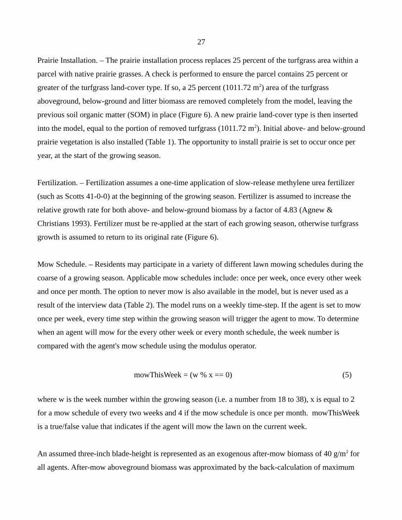
27
Prairie Installation. – The prairie installation process replaces 25 percent of the turfgrass area within a
parcel with native prairie grasses. A check is performed to ensure the parcel contains 25 percent or
greater of the turfgrass land-cover type. If so, a 25 percent (1011.72 m2) area of the turfgrass
aboveground, below-ground and litter biomass are removed completely from the model, leaving the
previous soil organic matter (SOM) in place (Figure 6). A new prairie land-cover type is then inserted
into the model, equal to the portion of removed turfgrass (1011.72 m2). Initial above- and below-ground
prairie vegetation is also installed (Table 1). The opportunity to install prairie is set to occur once per
year, at the start of the growing season.
Fertilization. – Fertilization assumes a one-time application of slow-release methylene urea fertilizer
(such as Scotts 41-0-0) at the beginning of the growing season. Fertilizer is assumed to increase the
relative growth rate for both above- and below-ground biomass by a factor of 4.83 (Agnew &
Christians 1993). Fertilizer must be re-applied at the start of each growing season, otherwise turfgrass
growth is assumed to return to its original rate (Figure 6).
Mow Schedule. – Residents may participate in a variety of different lawn mowing schedules during the
coarse of a growing season. Applicable mow schedules include: once per week, once every other week
and once per month. The option to never mow is also available in the model, but is never used as a
result of the interview data (Table 2). The model runs on a weekly time-step. If the agent is set to mow
once per week, every time step within the growing season will trigger the agent to mow. To determine
when an agent will mow for the every other week or every month schedule, the week number is
compared with the agent's mow schedule using the modulus operator.
mowThisWeek = (w % x == 0) (5)
where w is the week number within the growing season (i.e. a number from 18 to 38), x is equal to 2
for a mow schedule of every two weeks and 4 if the mow schedule is once per month. mowThisWeek
is a true/false value that indicates if the agent will mow the lawn on the current week.
An assumed three-inch blade-height is represented as an exogenous after-mow biomass of 40 g/m2 for
all agents. After-mow aboveground biomass was approximated by the back-calculation of maximum
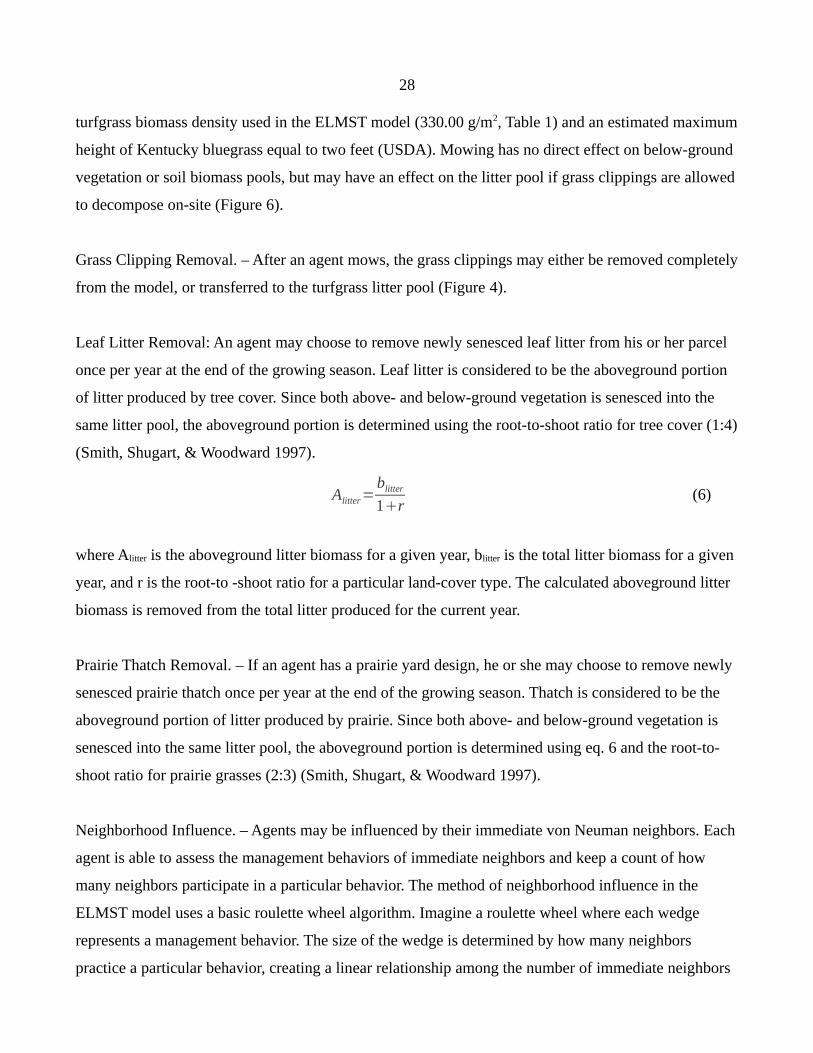
28
turfgrass biomass density used in the ELMST model (330.00 g/m2, Table 1) and an estimated maximum
height of Kentucky bluegrass equal to two feet (USDA). Mowing has no direct effect on below-ground
vegetation or soil biomass pools, but may have an effect on the litter pool if grass clippings are allowed
to decompose on-site (Figure 6).
Grass Clipping Removal. – After an agent mows, the grass clippings may either be removed completely
from the model, or transferred to the turfgrass litter pool (Figure 4).
Leaf Litter Removal: An agent may choose to remove newly senesced leaf litter from his or her parcel
once per year at the end of the growing season. Leaf litter is considered to be the aboveground portion
of litter produced by tree cover. Since both above- and below-ground vegetation is senesced into the
same litter pool, the aboveground portion is determined using the root-to-shoot ratio for tree cover (1:4)
(Smith, Shugart, & Woodward 1997).
Alitter=blitter
1r (6)
where Alitter is the aboveground litter biomass for a given year, blitter is the total litter biomass for a given
year, and r is the root-to -shoot ratio for a particular land-cover type. The calculated aboveground litter
biomass is removed from the total litter produced for the current year.
Prairie Thatch Removal. – If an agent has a prairie yard design, he or she may choose to remove newly
senesced prairie thatch once per year at the end of the growing season. Thatch is considered to be the
aboveground portion of litter produced by prairie. Since both above- and below-ground vegetation is
senesced into the same litter pool, the aboveground portion is determined using eq. 6 and the root-to-
shoot ratio for prairie grasses (2:3) (Smith, Shugart, & Woodward 1997).
Neighborhood Influence. – Agents may be influenced by their immediate von Neuman neighbors. Each
agent is able to assess the management behaviors of immediate neighbors and keep a count of how
many neighbors participate in a particular behavior. The method of neighborhood influence in the
ELMST model uses a basic roulette wheel algorithm. Imagine a roulette wheel where each wedge
represents a management behavior. The size of the wedge is determined by how many neighbors
practice a particular behavior, creating a linear relationship among the number of immediate neighbors

29
practicing a behavior and the likelihood of behavior adoption. During each time-step in the growing
season, an agent may assess the behaviors of her neighbors, construct a “mental roulette wheel” and
randomly select a behavior to adopt from the roulette wheel.
There are two caveats regarding the likelihood of adopting fertilization and prairie installation
behaviors as a result of neighborhood influence. While all other options (i.e. mow schedule, remove
grass clippings, remove fallen leaves and remove prairie thatch) are relatively simple behaviors in
practice, fertilization and prairie installation have additional associated costs. Fertilization requires the
resident to purchase fertilizer, apply it at the start of the growing season and the increased growth rate
of fertilized turfgrass remains for the duration of the growing season. Additional fertilization costs were
estimated do decrease the likelihood of fertilization adoption as a result of neighbor behaviors by a
“willingness to fertilize” factor of 0.50 (Table 2).
A similar situation occurs for the decision to install prairie. If a resident decides to install prairie, a
portion of turfgrass is removed and replaced with 1011.72 m2 of native prairie grasses (25 percent of the
parcel). The cost and planning necessary to install prairie is assumed to be higher than that of fertilizer
application. Moreover, once a prairie landscape is installed, it is considered permanent, and cannot be
reverted back to turfgrass, which bolsters the increased cost of prairie installation. As a result, a
“willingness to install prairie” factor is applied to prairie installation, decreasing the likelihood of
prairie adoption by a factor of 0.25 as a result of neighborhood influence (Table 2).
Statistical Analysis
The model was run 100 times under each research tier (Figure 1). Each run under a tier was
parameterized identically (Table 1, Table 2), with the exception of the random seed, which was
systematically incremented for each run. Management and neighborhood influence effects were
monitored across tiers. Total subdivision carbon was averaged over year 30 for each of the 100 in-tier
runs. Quantitative comparisons of total carbon storage at the subdivision level were made between each
tier using descriptive statistics and two-tailed Student's t-tests.
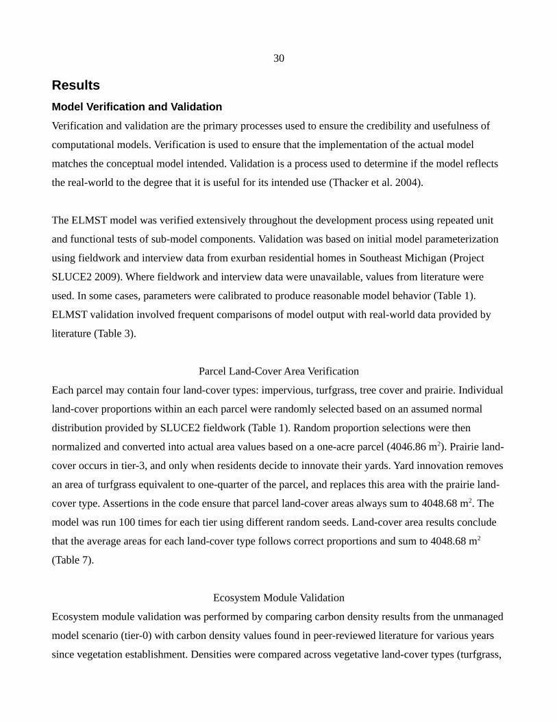
30
Results
Model Verification and Validation
Verification and validation are the primary processes used to ensure the credibility and usefulness of
computational models. Verification is used to ensure that the implementation of the actual model
matches the conceptual model intended. Validation is a process used to determine if the model reflects
the real-world to the degree that it is useful for its intended use (Thacker et al. 2004).
The ELMST model was verified extensively throughout the development process using repeated unit
and functional tests of sub-model components. Validation was based on initial model parameterization
using fieldwork and interview data from exurban residential homes in Southeast Michigan (Project
SLUCE2 2009). Where fieldwork and interview data were unavailable, values from literature were
used. In some cases, parameters were calibrated to produce reasonable model behavior (Table 1).
ELMST validation involved frequent comparisons of model output with real-world data provided by
literature (Table 3).
Parcel Land-Cover Area Verification
Each parcel may contain four land-cover types: impervious, turfgrass, tree cover and prairie. Individual
land-cover proportions within an each parcel were randomly selected based on an assumed normal
distribution provided by SLUCE2 fieldwork (Table 1). Random proportion selections were then
normalized and converted into actual area values based on a one-acre parcel (4046.86 m2). Prairie land-
cover occurs in tier-3, and only when residents decide to innovate their yards. Yard innovation removes
an area of turfgrass equivalent to one-quarter of the parcel, and replaces this area with the prairie land-
cover type. Assertions in the code ensure that parcel land-cover areas always sum to 4048.68 m2. The
model was run 100 times for each tier using different random seeds. Land-cover area results conclude
that the average areas for each land-cover type follows correct proportions and sum to 4048.68 m2
(Table 7).
Ecosystem Module Validation
Ecosystem module validation was performed by comparing carbon density results from the unmanaged
model scenario (tier-0) with carbon density values found in peer-reviewed literature for various years
since vegetation establishment. Densities were compared across vegetative land-cover types (turfgrass,
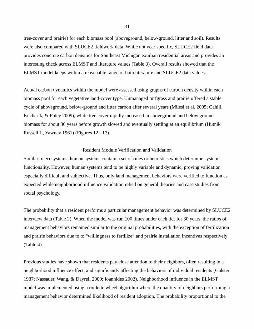
31
tree-cover and prairie) for each biomass pool (aboveground, below-ground, litter and soil). Results
were also compared with SLUCE2 fieldwork data. While not year specific, SLUCE2 field data
provides concrete carbon densities for Southeast Michigan exurban residential areas and provides an
interesting check across ELMST and literature values (Table 3). Overall results showed that the
ELMST model keeps within a reasonable range of both literature and SLUCE2 data values.
Actual carbon dynamics within the model were assessed using graphs of carbon density within each
biomass pool for each vegetative land-cover type. Unmanaged turfgrass and prairie offered a stable
cycle of aboveground, below-ground and litter carbon after several years (Milesi et al. 2005; Cahill,
Kucharik, & Foley 2009), while tree cover rapidly increased in aboveground and below ground
biomass for about 30 years before growth slowed and eventually settling at an equilibrium (Hutnik
Russell J., Yawney 1961) (Figures 12 - 17).
Resident Module Verification and Validation
Similar to ecosystems, human systems contain a set of rules or heuristics which determine system
functionality. However, human systems tend to be highly variable and dynamic, proving validation
especially difficult and subjective. Thus, only land management behaviors were verified to function as
expected while neighborhood influence validation relied on general theories and case studies from
social psychology.
The probability that a resident performs a particular management behavior was determined by SLUCE2
interview data (Table 2). When the model was run 100 times under each tier for 30 years, the ratios of
management behaviors remained similar to the original probabilities, with the exception of fertilization
and prairie behaviors due to to “willingness to fertilize” and prairie installation incentives respectively
(Table 4).
Previous studies have shown that residents pay close attention to their neighbors, often resulting in a
neighborhood influence effect, and significantly affecting the behaviors of individual residents (Galster
1987; Nassauer, Wang, & Dayrell 2009; Ioannides 2002). Neighborhood influence in the ELMST
model was implemented using a roulette wheel algorithm where the quantity of neighbors performing a
management behavior determined likelihood of resident adoption. The probability proportional to the

32
number of neighbors performing a behavior provided a reasonable guess as to the details of the
neighborhood influence mechanism. Thus, the roulette wheel algorithm can be used in a computational
experiment that reveals how the total subdivision carbon would behave if proportional selection was a
correct assumption (Bankes 1993).
Effect of Individual Management Behaviors
The differential effect of each individual management behavior on the outcome of total carbon at the
subdivision level was evaluated. Testing the effect of individual behaviors assumed the standard 9x9
subdivision used in this study. All agents were set to perform a single management task consistently for
the duration of the model run. Total carbon in the subdivision (measured in Mg C) was recorded for the
ten years between year 25 and 35 of the model (Figure 9; Table 5). The effect of individual
management behaviors provided insight into outcomes with heterogeneous agents, parcels and
neighborhood influence effects.
Model results show that fertilization has the greatest positive effect, increasing the total carbon in an
unmanaged subdivision by approximately 40 percent on average, relative to unmanaged parcels.
Mowing the lawn and leaving the grass clippings to decompose on-site and may also increase the total
carbon in the model by about 17 to 20 percent, relative to the unmanaged scenario, as does having one-
quarter of every parcel in native prairie and allowing the thatch to decompose on-site. Removing grass
clippings after mowing significantly decreases the amount of carbon in a subdivision by roughly 40 to
44 percent when compared with no management. Removing fallen leaves and prairie thatch has less of
an effect, decreasing the modeled carbon storage by approximately 4 to 7 percent relative to the
unmanaged scenario.
Model Application
The model was applied using the four tier-based research scenarios as illustrated in Figure 1. In this
section, results for each tier are described, followed by a comparison among tiers used to test research
hypothesis.
Tier-0 – No Management
When a conventional subdivision is developed and no management takes place over a span of 30 years,

33
the total carbon in the subdivision is deterministic because the rules that determine growth, senescence,
litter decay and respiration remain constant. Year 30 model results yield a carbon store range from 234
to 272 Mg C with an average of 255 (± 8.13) Mg C. The low variability in this case is due to annual
seasonal shifts in growth, senescence, litter decay and respiration.
Tier-1 – Intrinsic Management
The tier-1 model scenario involves a developed conventional subdivision where residents manage
vegetation and litter according to their intrinsic preferences, without adaptation and without
neighborhood influence. In this scenario, the total carbon in the subdivision is also deterministic
because the rules that determine growth, senescence, litter decay and respiration remain constant as do
management behaviors. Year 30 model results yield a carbon store range from 399 to 568 Mg C with an
average of 487 (± 31) Mg C. The variability in this scenario is due to the interaction of annual seasonal
shifts in natural processes (growth, senescence, litter decay and respiration) and intrinsic land
management behaviors of fertilization, lawn mowing, and grass clipping or leaf removal. Prairie is not
assumed to be present in this scenario.
Tier-2 – Adaptive Management
In the tier-2 ELMST scenario, a conventional subdivision is developed and residents manage
vegetation and litter according to their intrinsic preferences, but also have the ability to influence one
another. With the ability to adopt new management behaviors over a 30 year span, the total carbon in
the subdivision depended on emergent local norms resulting from neighborhood influence. Year 30
model results yield a carbon store range from 182 to 586 Mg C with an average of 387 (± 75) Mg C.
The variability in this case was due to the interaction of annual seasonal shifts in natural processes
(growth, senescence, litter decay and respiration), land management behaviors (fertilization, lawn
mowing, and grass clipping or leaf removal) and management adaptation based on the behaviors of a
resident's immediate von Neuman neighbors. Prairie is not assumed to be present in the tier-2 scenario.
Tier-3 – Adaptive Management with Incentive to Innovate
In tier-3, approximately four percent (three out of eighty-one) residents in a conventional subdivision
accept an incentive to innovate their yards from a conventional turfgrass design to a 25 percent native
prairie design (Table 7); residents manage their yards and are responsive to the management behaviors
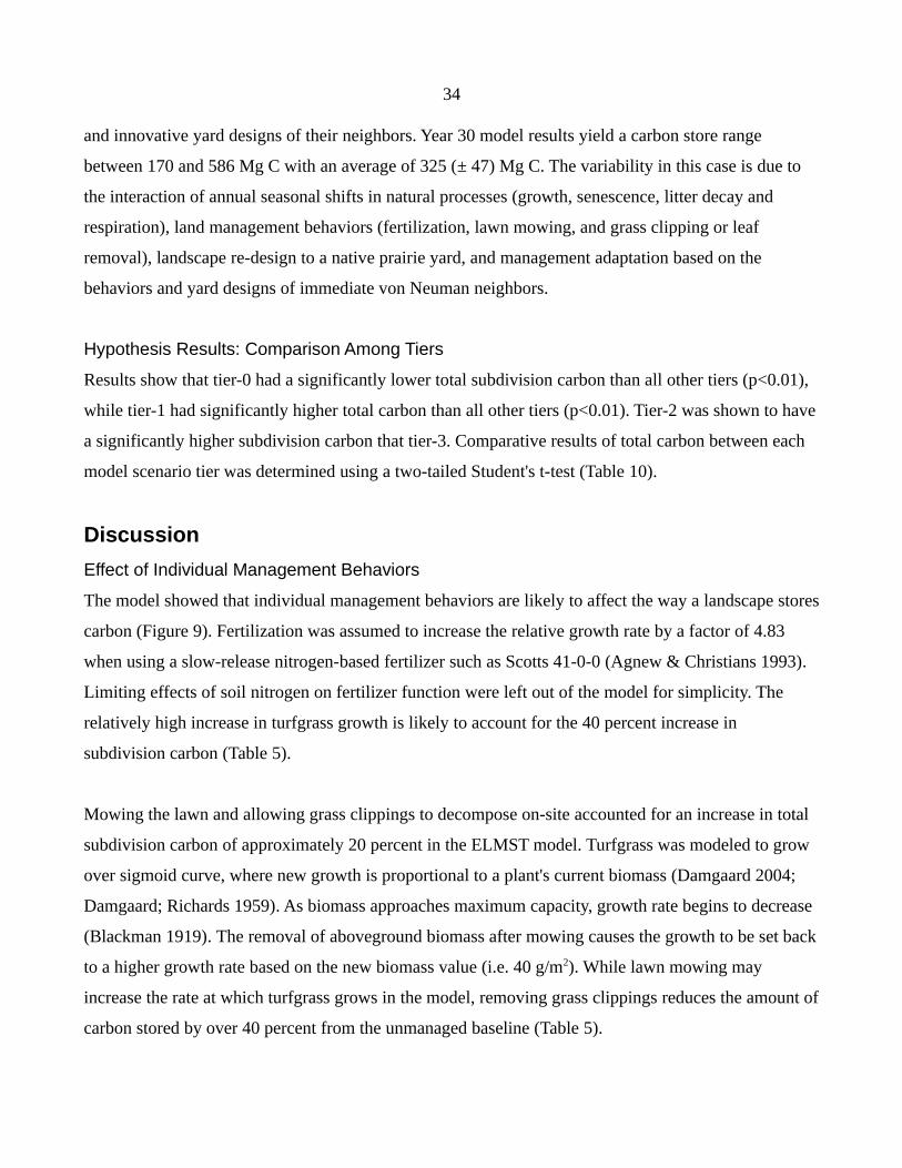
34
and innovative yard designs of their neighbors. Year 30 model results yield a carbon store range
between 170 and 586 Mg C with an average of 325 (± 47) Mg C. The variability in this case is due to
the interaction of annual seasonal shifts in natural processes (growth, senescence, litter decay and
respiration), land management behaviors (fertilization, lawn mowing, and grass clipping or leaf
removal), landscape re-design to a native prairie yard, and management adaptation based on the
behaviors and yard designs of immediate von Neuman neighbors.
Hypothesis Results: Comparison Among Tiers
Results show that tier-0 had a significantly lower total subdivision carbon than all other tiers (p<0.01),
while tier-1 had significantly higher total carbon than all other tiers (p<0.01). Tier-2 was shown to have
a significantly higher subdivision carbon that tier-3. Comparative results of total carbon between each
model scenario tier was determined using a two-tailed Student's t-test (Table 10).
Discussion
Effect of Individual Management Behaviors
The model showed that individual management behaviors are likely to affect the way a landscape stores
carbon (Figure 9). Fertilization was assumed to increase the relative growth rate by a factor of 4.83
when using a slow-release nitrogen-based fertilizer such as Scotts 41-0-0 (Agnew & Christians 1993).
Limiting effects of soil nitrogen on fertilizer function were left out of the model for simplicity. The
relatively high increase in turfgrass growth is likely to account for the 40 percent increase in
subdivision carbon (Table 5).
Mowing the lawn and allowing grass clippings to decompose on-site accounted for an increase in total
subdivision carbon of approximately 20 percent in the ELMST model. Turfgrass was modeled to grow
over sigmoid curve, where new growth is proportional to a plant's current biomass (Damgaard 2004;
Damgaard; Richards 1959). As biomass approaches maximum capacity, growth rate begins to decrease
(Blackman 1919). The removal of aboveground biomass after mowing causes the growth to be set back
to a higher growth rate based on the new biomass value (i.e. 40 g/m2). While lawn mowing may
increase the rate at which turfgrass grows in the model, removing grass clippings reduces the amount of
carbon stored by over 40 percent from the unmanaged baseline (Table 5).
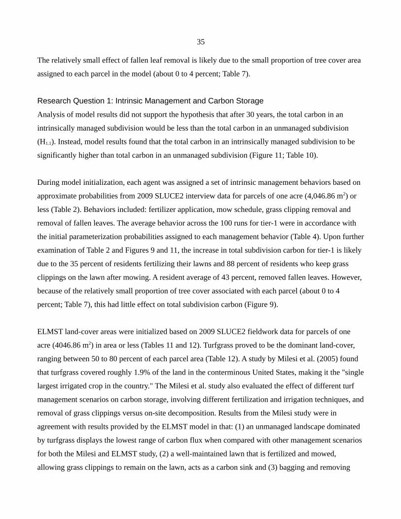
35
The relatively small effect of fallen leaf removal is likely due to the small proportion of tree cover area
assigned to each parcel in the model (about 0 to 4 percent; Table 7).
Research Question 1: Intrinsic Management and Carbon Storage
Analysis of model results did not support the hypothesis that after 30 years, the total carbon in an
intrinsically managed subdivision would be less than the total carbon in an unmanaged subdivision
(H1.1). Instead, model results found that the total carbon in an intrinsically managed subdivision to be
significantly higher than total carbon in an unmanaged subdivision (Figure 11; Table 10).
During model initialization, each agent was assigned a set of intrinsic management behaviors based on
approximate probabilities from 2009 SLUCE2 interview data for parcels of one acre (4,046.86 m2) or
less (Table 2). Behaviors included: fertilizer application, mow schedule, grass clipping removal and
removal of fallen leaves. The average behavior across the 100 runs for tier-1 were in accordance with
the initial parameterization probabilities assigned to each management behavior (Table 4). Upon further
examination of Table 2 and Figures 9 and 11, the increase in total subdivision carbon for tier-1 is likely
due to the 35 percent of residents fertilizing their lawns and 88 percent of residents who keep grass
clippings on the lawn after mowing. A resident average of 43 percent, removed fallen leaves. However,
because of the relatively small proportion of tree cover associated with each parcel (about 0 to 4
percent; Table 7), this had little effect on total subdivision carbon (Figure 9).
ELMST land-cover areas were initialized based on 2009 SLUCE2 fieldwork data for parcels of one
acre (4046.86 m2) in area or less (Tables 11 and 12). Turfgrass proved to be the dominant land-cover,
ranging between 50 to 80 percent of each parcel area (Table 12). A study by Milesi et al. (2005) found
that turfgrass covered roughly 1.9% of the land in the conterminous United States, making it the "single
largest irrigated crop in the country." The Milesi et al. study also evaluated the effect of different turf
management scenarios on carbon storage, involving different fertilization and irrigation techniques, and
removal of grass clippings versus on-site decomposition. Results from the Milesi study were in
agreement with results provided by the ELMST model in that: (1) an unmanaged landscape dominated
by turfgrass displays the lowest range of carbon flux when compared with other management scenarios
for both the Milesi and ELMST study, (2) a well-maintained lawn that is fertilized and mowed,
allowing grass clippings to remain on the lawn, acts as a carbon sink and (3) bagging and removing

36
grass clippings reduces overall carbon storage (Milesi et al. 2005)(Figure 9, Figure 11).
Result from the model showed that intrinsic management of residential parcels in conventional exurban
subdivisions in Southeast Michigan may store nearly twice the carbon than unmanaged subdivision
after 30 years (Table 10). The intrinsic management scenario (tier-1) relies on initial allocation of
management behaviors, which do not change over time. The outcome of tier-1 is therefore,
deterministic given the initial agent behaviors and ecosystem variables. Model results found that the
variability of carbon storage from an intrinsically managed subdivision over year 30 is also greater than
that of an unmanaged subdivision. Greater variability is most likely be due to the manual alteration of
carbon mean resident time (MRT) within each biomass pool through the various intrinsic management
behaviors. Moreover, the greater total carbon in a managed subdivision (tier-1) may be due to the
majority of agents mowing their lawns and leaving the grass clippings to decompose on-site. In
addition, 35 percent of residents fertilize their lawn, which dramatically increases the affect on total
subdivision carbon (Figure 9, Table 5).
Research Question 2: Adaptive Management and Carbon Storage
Model results did not support either hypothesis for a subdivision having neighborhood influence (H2.1
and H2.2). Results showed that the total carbon in a subdivision having neighborhood influence (tier-2)
to be significantly higher than an unmanaged subdivision (tier-0), and significantly lower than a
managed subdivision without neighborhood influence (tier-1), however tier-2 had the largest variability
of total subdivision carbon over the 100 model runs (Figure 11; Table 10).
Total subdivision carbon among individual model runs varied greatly. This variance is likely due to the
assortment of “management cultures” that emerged through the process of neighborhood influence. For
example, in one model run, removing leaf litter may have been adopted as a subdivision norm, while
another model run may have demonstrated a subdivision where most residents allow leaf litter to
remain on their individual parcels. When behaviors were averaged among the model runs over 30
years, results showed overall behaviors to remain relatively stable, with the exception of fertilizer
application, which dropped from 35 percent of the residents to zero residents after 30 years.
The zero percent fertilization result in tiers-2 and -3 is due to the willingness to fertilize parameter
(Table 2). Willingness to fertilize was set to a best-guess assumption of 0.50 and applied during the

37
neighborhood influence process to reflect a higher cost of adopting the fertilization behavior. For
example, switching lawn mowing schedules, or deciding to remove fallen leaves at the end of the
growing season are associated with the relatively low costs for adopting the new behavior. Adopting a
fertilization regimen, however, accrues the cost of buying fertilizer, applying the fertilizer, and the
commitment of always having a fertilized lawn for the remainder of the growing season. External
social stigmas regarding the environmental effects of fertilizer application may also play into a
resident's willingness to fertilize. The willingness to fertilize parameter was set such that the likelihood
of a resident to adopt the fertilization behavior to be half that of other management behavior adoption
probabilities in tier-2 and tier-3. Willingness to fertilize was the same for all residents, and remained
constant throughout each model run. Sensitivity analysis showed agent adoption of fertilization
behavior to be highly sensitive to the willingness to fertilize parameter implementation. Results showed
that if willingness to fertilize is less-than one, the number of residents who fertilized their lawn will
decrease over time; the lower the willingness to fertilize, the faster the decrease in the number of
residents who fertilize. After 30 years, the model showed the number of residents who fertilized their
lawns to be zero for all 100 runs at the set willingness to fertilize value of 0.5 (Table 4).
The present model implementation found that when neighborhood influence is applied to a
conventional residential exurban subdivision initialized with interview and field data from Southeast
Michigan, the subdivision may store either more or less carbon than an unmanaged subdivision after 30
years (Figure 11), depending on the local norms which emerged from neighborhood influence of
management behaviors. In most cases, the model found that the subdivision will store more carbon than
an unmanaged subdivision, even with infrequent lawn fertilization.
As with tier-1, tier-2 relies on the initial distribution of management behaviors as a starting point for
subdivision evolution. Through the process of neighborhood influence, emergent local norms relating
to yard management behaviors are likely to cause a carbon trajectory lock-in at the levels of the
biomass pools, land-covers and subdivision. Whereas the carbon-trajectory for tiers -0 and -1 were
locked-in from the start, the trajectory for tier-2 was erratic for the first few years, before finally
stabilizing as resident management converged into a local norm (Figure 32 - 39). The ELMST model
showed that neighborhood influence allows for a wide range of carbon trajectory lock-ins as illustrated
by Figure 11.
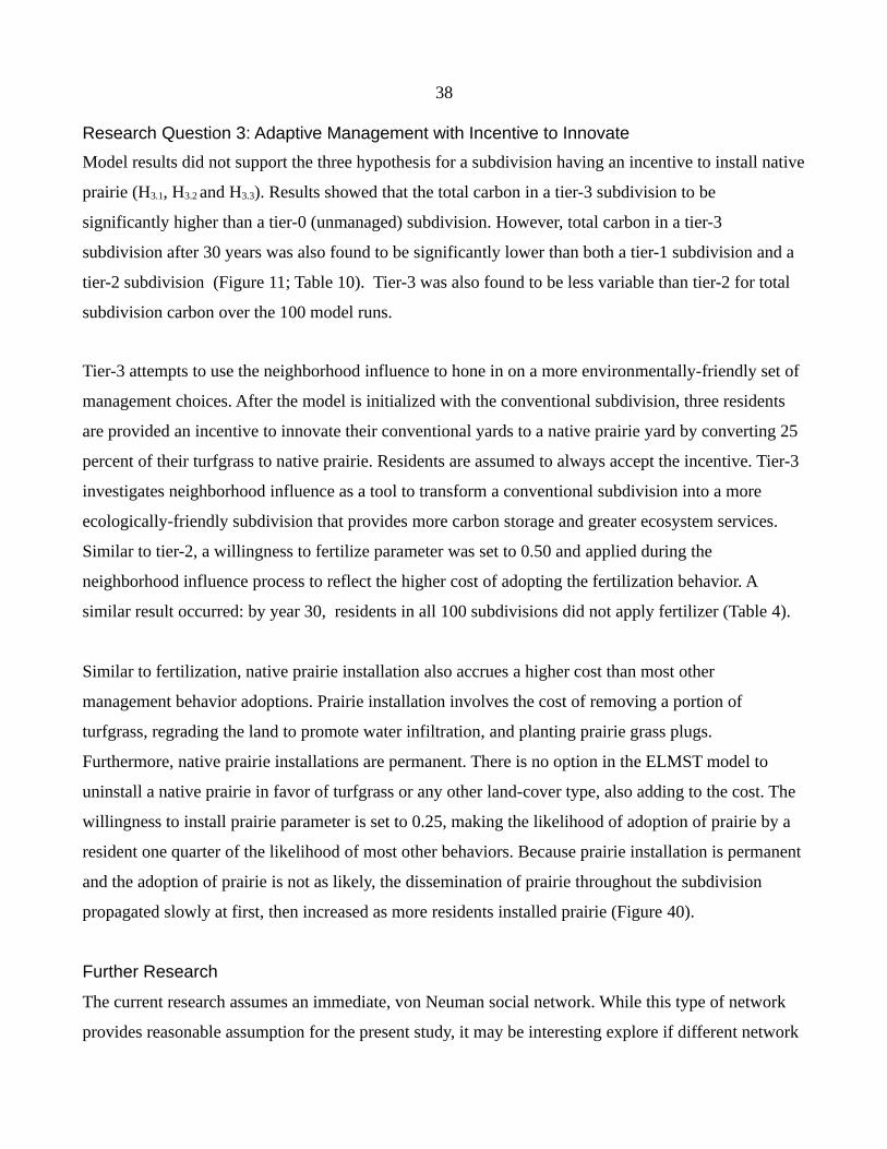
38
Research Question 3: Adaptive Management with Incentive to Innovate
Model results did not support the three hypothesis for a subdivision having an incentive to install native
prairie (H3.1, H3.2 and H3.3). Results showed that the total carbon in a tier-3 subdivision to be
significantly higher than a tier-0 (unmanaged) subdivision. However, total carbon in a tier-3
subdivision after 30 years was also found to be significantly lower than both a tier-1 subdivision and a
tier-2 subdivision (Figure 11; Table 10). Tier-3 was also found to be less variable than tier-2 for total
subdivision carbon over the 100 model runs.
Tier-3 attempts to use the neighborhood influence to hone in on a more environmentally-friendly set of
management choices. After the model is initialized with the conventional subdivision, three residents
are provided an incentive to innovate their conventional yards to a native prairie yard by converting 25
percent of their turfgrass to native prairie. Residents are assumed to always accept the incentive. Tier-3
investigates neighborhood influence as a tool to transform a conventional subdivision into a more
ecologically-friendly subdivision that provides more carbon storage and greater ecosystem services.
Similar to tier-2, a willingness to fertilize parameter was set to 0.50 and applied during the
neighborhood influence process to reflect the higher cost of adopting the fertilization behavior. A
similar result occurred: by year 30, residents in all 100 subdivisions did not apply fertilizer (Table 4).
Similar to fertilization, native prairie installation also accrues a higher cost than most other
management behavior adoptions. Prairie installation involves the cost of removing a portion of
turfgrass, regrading the land to promote water infiltration, and planting prairie grass plugs.
Furthermore, native prairie installations are permanent. There is no option in the ELMST model to
uninstall a native prairie in favor of turfgrass or any other land-cover type, also adding to the cost. The
willingness to install prairie parameter is set to 0.25, making the likelihood of adoption of prairie by a
resident one quarter of the likelihood of most other behaviors. Because prairie installation is permanent
and the adoption of prairie is not as likely, the dissemination of prairie throughout the subdivision
propagated slowly at first, then increased as more residents installed prairie (Figure 40).
Further Research
The current research assumes an immediate, von Neuman social network. While this type of network
provides reasonable assumption for the present study, it may be interesting explore if different network
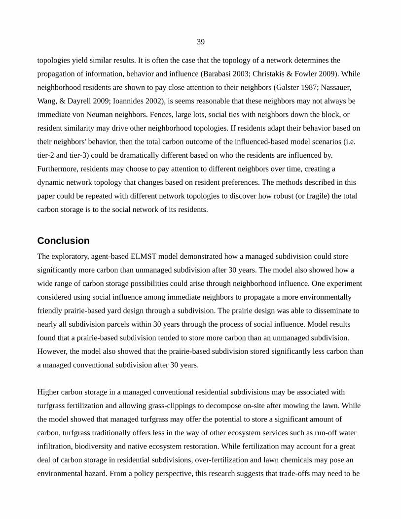
39
topologies yield similar results. It is often the case that the topology of a network determines the
propagation of information, behavior and influence (Barabasi 2003; Christakis & Fowler 2009). While
neighborhood residents are shown to pay close attention to their neighbors (Galster 1987; Nassauer,
Wang, & Dayrell 2009; Ioannides 2002), is seems reasonable that these neighbors may not always be
immediate von Neuman neighbors. Fences, large lots, social ties with neighbors down the block, or
resident similarity may drive other neighborhood topologies. If residents adapt their behavior based on
their neighbors' behavior, then the total carbon outcome of the influenced-based model scenarios (i.e.
tier-2 and tier-3) could be dramatically different based on who the residents are influenced by.
Furthermore, residents may choose to pay attention to different neighbors over time, creating a
dynamic network topology that changes based on resident preferences. The methods described in this
paper could be repeated with different network topologies to discover how robust (or fragile) the total
carbon storage is to the social network of its residents.
Conclusion
The exploratory, agent-based ELMST model demonstrated how a managed subdivision could store
significantly more carbon than unmanaged subdivision after 30 years. The model also showed how a
wide range of carbon storage possibilities could arise through neighborhood influence. One experiment
considered using social influence among immediate neighbors to propagate a more environmentally
friendly prairie-based yard design through a subdivision. The prairie design was able to disseminate to
nearly all subdivision parcels within 30 years through the process of social influence. Model results
found that a prairie-based subdivision tended to store more carbon than an unmanaged subdivision.
However, the model also showed that the prairie-based subdivision stored significantly less carbon than
a managed conventional subdivision after 30 years.
Higher carbon storage in a managed conventional residential subdivisions may be associated with
turfgrass fertilization and allowing grass-clippings to decompose on-site after mowing the lawn. While
the model showed that managed turfgrass may offer the potential to store a significant amount of
carbon, turfgrass traditionally offers less in the way of other ecosystem services such as run-off water
infiltration, biodiversity and native ecosystem restoration. While fertilization may account for a great
deal of carbon storage in residential subdivisions, over-fertilization and lawn chemicals may pose an
environmental hazard. From a policy perspective, this research suggests that trade-offs may need to be

40
considered when determining between carbon storage and other ecosystem services in residential
landscapes.
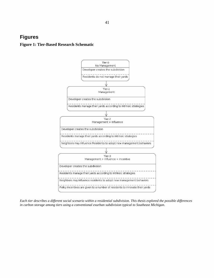
41
FiguresFigure 1: Tier-Based Research Schematic
Each tier describes a different social scenario within a residential subdivision. This thesis explored the possible differences in carbon storage among tiers using a conventional exurban subdivision typical to Southeast Michigan.
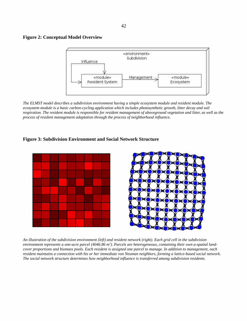
42
Figure 2: Conceptual Model Overview
The ELMST model describes a subdivision environment having a simple ecosystem module and resident module. The ecosystem module is a basic carbon-cycling application which includes photosynthetic growth, litter decay and soil respiration. The resident module is responsible for resident management of aboveground vegetation and litter, as well as the process of resident management adaptation through the process of neighborhood influence.
Figure 3: Subdivision Environment and Social Network Structure
An illustration of the subdivision environment (left) and resident network (right). Each grid cell in the subdivision environment represents a one-acre parcel (4046.86 m2). Parcels are heterogeneous, containing their own a-spatial land-cover proportions and biomass pools. Each resident is assigned one parcel to manage. In addition to management, each resident maintains a connection with his or her immediate von Neuman neighbors, forming a lattice-based social network. The social network structure determines how neighborhood influence is transferred among subdivision residents.
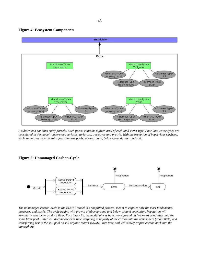
43
Figure 4: Ecosystem Components
A subdivision contains many parcels. Each parcel contains a given area of each land-cover type. Four land-cover types are considered in the model: impervious surfaces, turfgrass, tree cover and prairie. With the exception of impervious surfaces, each land-cover type contains four biomass pools: aboveground, below-ground, litter and soil.
Figure 5: Unmanaged Carbon-Cycle
The unmanaged carbon-cycle in the ELMST model is a simplified process, meant to capture only the most fundamental processes and stocks. The cycle begins with growth of aboveground and below-ground vegetation. Vegetation will eventually senesce to produce litter. For simplicity, the model places both aboveground and below-ground litter into the same litter pool. Litter will decompose over time, respiring a majority of the carbon into the atmosphere (about 80%) and transferring rest to the soil pool as soil organic matter (SOM). Over time, soil will slowly respire carbon back into the atmosphere.
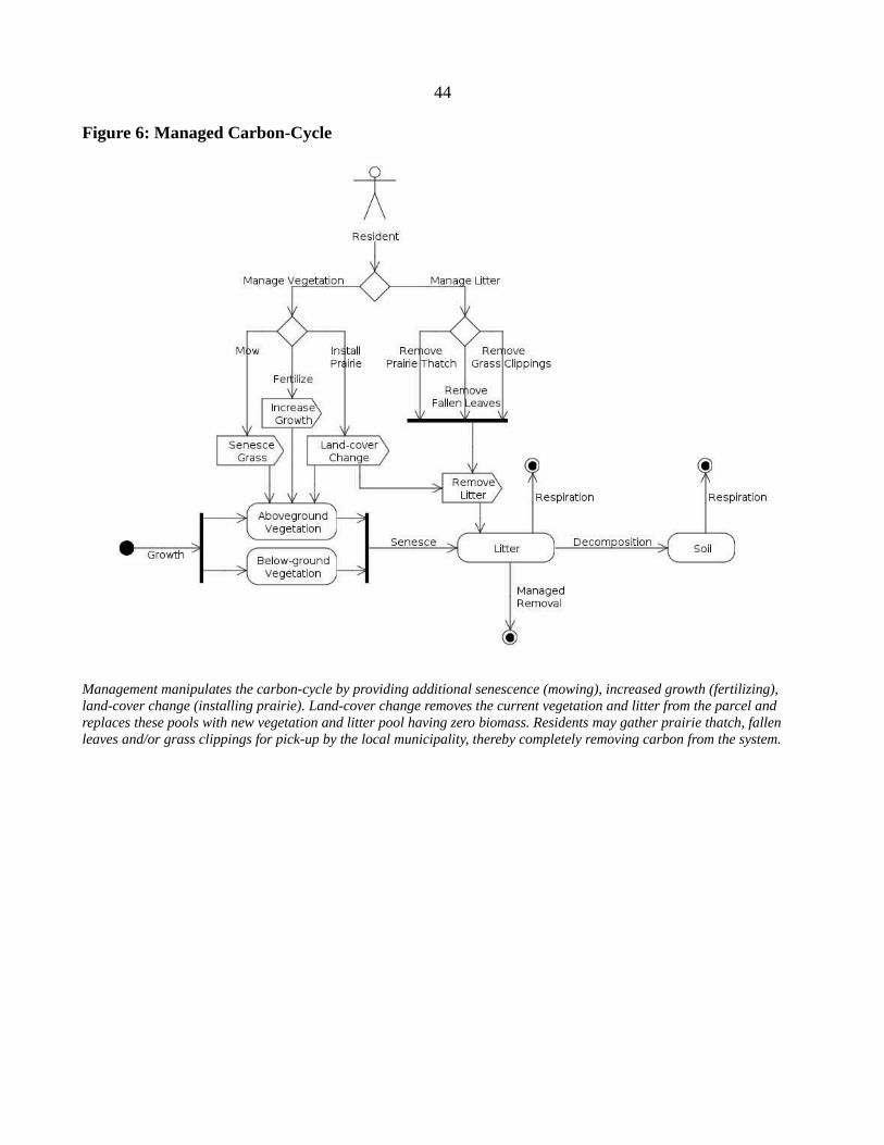
44
Figure 6: Managed Carbon-Cycle
Management manipulates the carbon-cycle by providing additional senescence (mowing), increased growth (fertilizing), land-cover change (installing prairie). Land-cover change removes the current vegetation and litter from the parcel and replaces these pools with new vegetation and litter pool having zero biomass. Residents may gather prairie thatch, fallen leaves and/or grass clippings for pick-up by the local municipality, thereby completely removing carbon from the system.
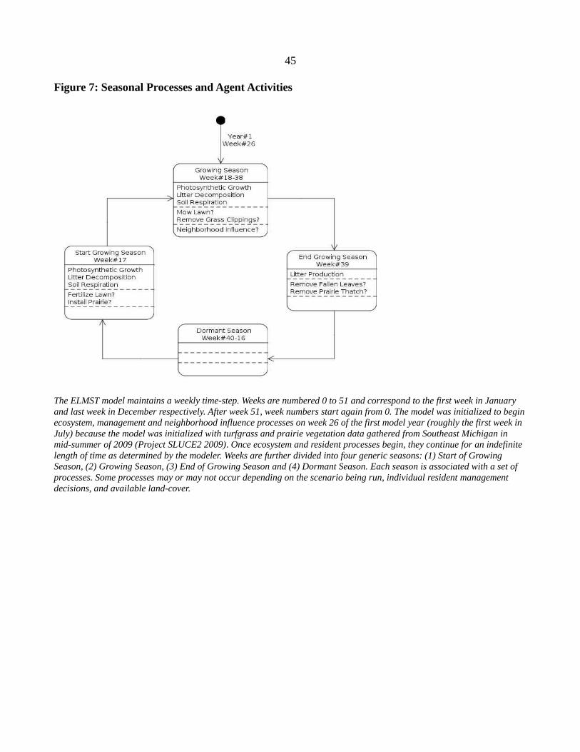
45
Figure 7: Seasonal Processes and Agent Activities
The ELMST model maintains a weekly time-step. Weeks are numbered 0 to 51 and correspond to the first week in January and last week in December respectively. After week 51, week numbers start again from 0. The model was initialized to begin ecosystem, management and neighborhood influence processes on week 26 of the first model year (roughly the first week in July) because the model was initialized with turfgrass and prairie vegetation data gathered from Southeast Michigan in mid-summer of 2009 (Project SLUCE2 2009). Once ecosystem and resident processes begin, they continue for an indefinite length of time as determined by the modeler. Weeks are further divided into four generic seasons: (1) Start of Growing Season, (2) Growing Season, (3) End of Growing Season and (4) Dormant Season. Each season is associated with a set of processes. Some processes may or may not occur depending on the scenario being run, individual resident management decisions, and available land-cover.
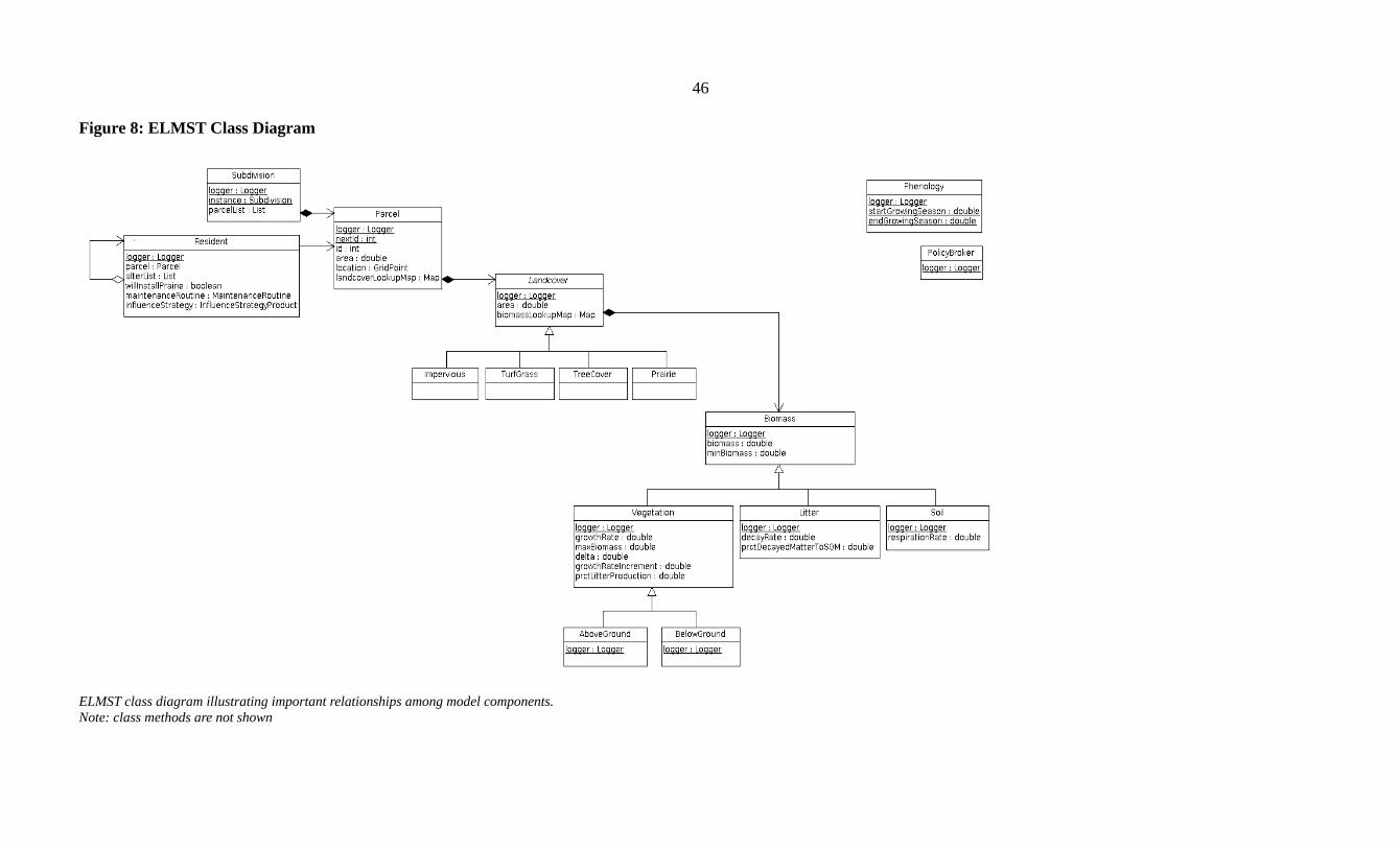
46
Figure 8: ELMST Class Diagram
ELMST class diagram illustrating important relationships among model components.Note: class methods are not shown
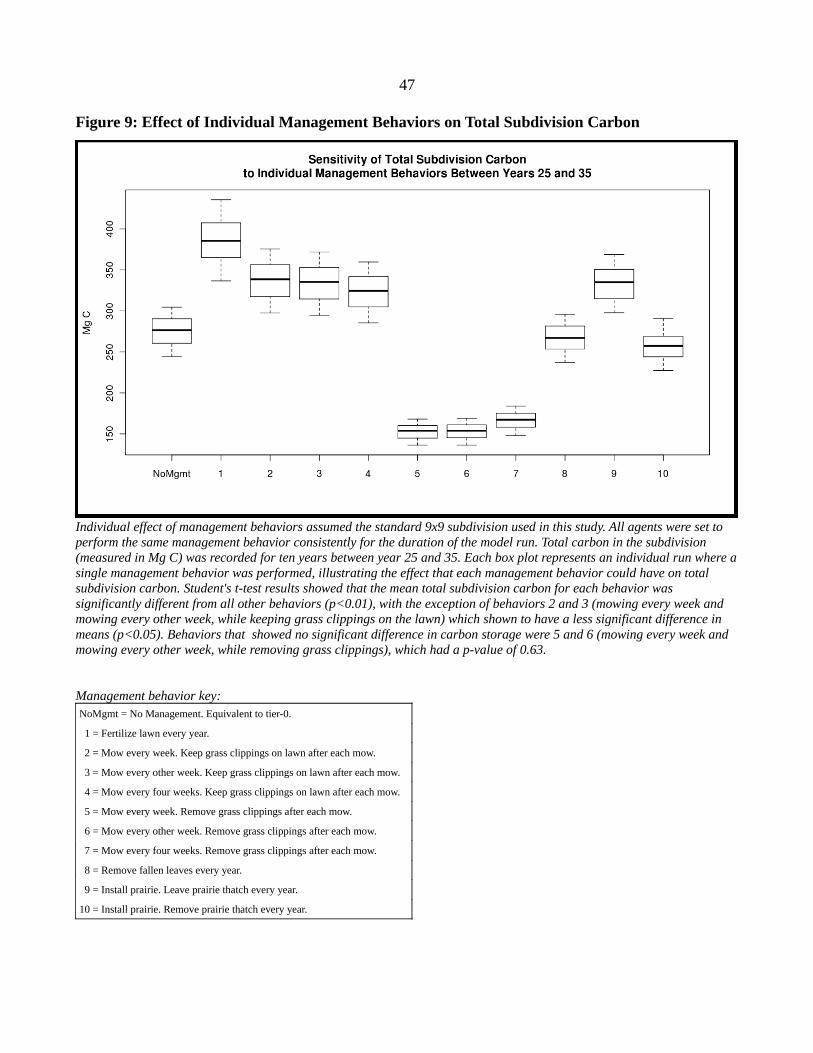
47
Figure 9: Effect of Individual Management Behaviors on Total Subdivision Carbon
Individual effect of management behaviors assumed the standard 9x9 subdivision used in this study. All agents were set to perform the same management behavior consistently for the duration of the model run. Total carbon in the subdivision (measured in Mg C) was recorded for ten years between year 25 and 35. Each box plot represents an individual run where a single management behavior was performed, illustrating the effect that each management behavior could have on total subdivision carbon. Student's t-test results showed that the mean total subdivision carbon for each behavior was significantly different from all other behaviors (p<0.01), with the exception of behaviors 2 and 3 (mowing every week and mowing every other week, while keeping grass clippings on the lawn) which shown to have a less significant difference in means (p<0.05). Behaviors that showed no significant difference in carbon storage were 5 and 6 (mowing every week and mowing every other week, while removing grass clippings), which had a p-value of 0.63.
Management behavior key:NoMgmt = No Management. Equivalent to tier-0.
1 = Fertilize lawn every year.
2 = Mow every week. Keep grass clippings on lawn after each mow.
3 = Mow every other week. Keep grass clippings on lawn after each mow.
4 = Mow every four weeks. Keep grass clippings on lawn after each mow.
5 = Mow every week. Remove grass clippings after each mow.
6 = Mow every other week. Remove grass clippings after each mow.
7 = Mow every four weeks. Remove grass clippings after each mow.
8 = Remove fallen leaves every year.
9 = Install prairie. Leave prairie thatch every year.
10 = Install prairie. Remove prairie thatch every year.
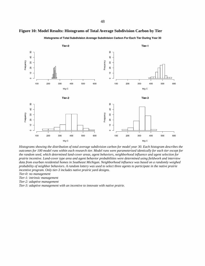
48
Figure 10: Model Results: Histograms of Total Average Subdivision Carbon by Tier
Histograms showing the distribution of total average subdivision carbon for model year 30. Each histogram describes the outcomes for 100 model runs within each research tier. Model runs were parameterized identically for each tier except for the random seed, which determined land-cover areas, agent behaviors, neighborhood influence and agent selection for prairie incentive. Land-cover type area and agent behavior probabilities were determined using fieldwork and interview data from exurban residential homes in Southeast Michigan. Neighborhood influence was based on a randomly weighed probability of neighbor behaviors. A random lottery was used to select three agents to participate in the native prairie incentive program. Only tier-3 includes native prairie yard designs. Tier-0: no managementTier-1: intrinsic managementTier-2: adaptive managementTier-3: adaptive management with an incentive to innovate with native prairie.

49
Figure 11: Model Results: Box Plot of Total Average Subdivision Carbon by Tier
Box plot showing the distribution of total average subdivision carbon for model year 30. Each distribution shows the range of outcomes for 100 model runs within each research tier. Model runs were parameterized identically for each tier except for the random seed, which determined land-cover areas, agent behaviors, neighborhood influence and agent selection for prairie incentive. Land-cover type area and agent behavior probabilities were determined using fieldwork and interview data from exurban residential homes in Southeast Michigan. Neighborhood influence was based on a randomly weighed probability of neighbor behaviors. A random lottery was used to select three agents to participate in the native prairie incentive program. Only tier-3 includes native prairie yard designs. Tier-0: no managementTier-1: intrinsic managementTier-2: adaptive managementTier-3: adaptive management with an incentive to innovate with native prairie.
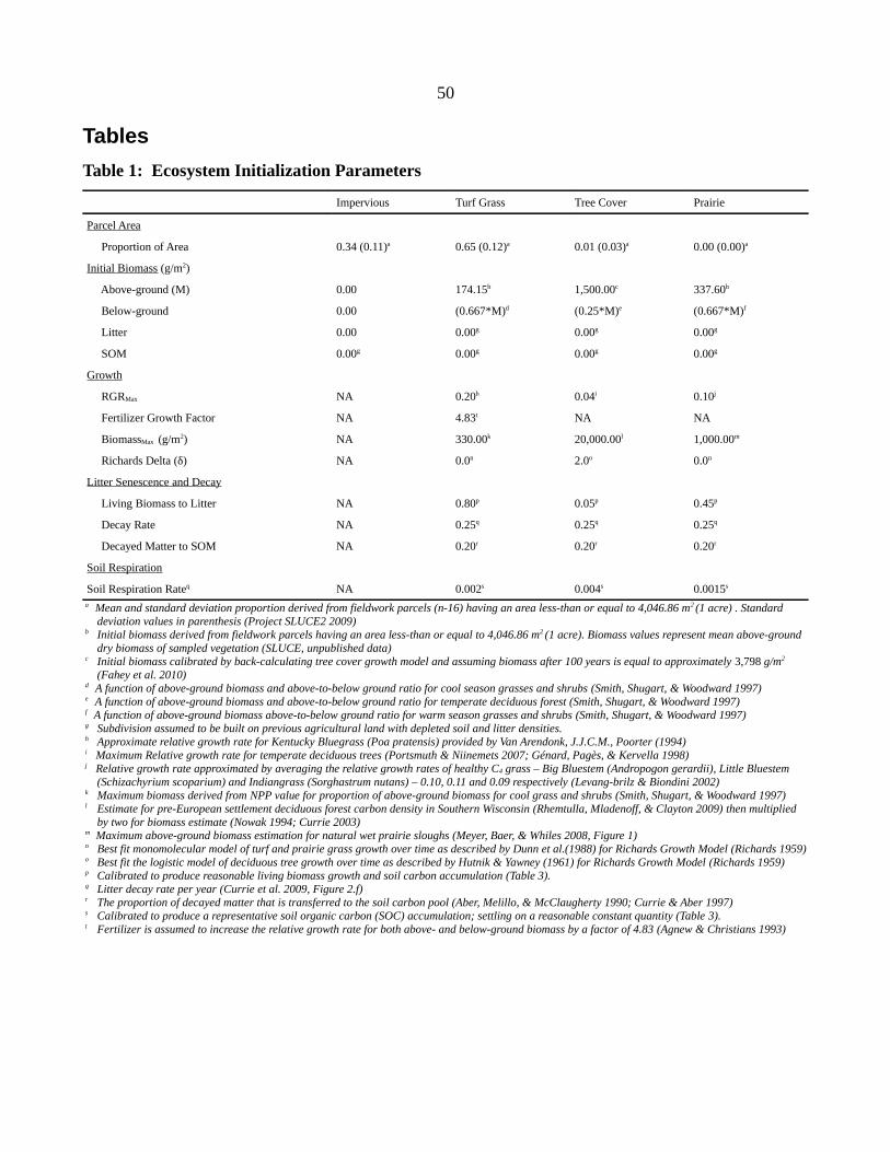
50
Tables
Table 1: Ecosystem Initialization Parameters
Impervious Turf Grass Tree Cover Prairie
Parcel Area
Proportion of Area 0.34 (0.11)a 0.65 (0.12)a 0.01 (0.03)a 0.00 (0.00)a
Initial Biomass (g/m2)
Above-ground (M) 0.00 174.15b 1,500.00c 337.60b
Below-ground 0.00 (0.667*M)d (0.25*M)e (0.667*M)f
Litter 0.00 0.00g 0.00g 0.00g
SOM 0.00g 0.00g 0.00g 0.00g
Growth
RGRMax NA 0.20h 0.04i 0.10j
Fertilizer Growth Factor NA 4.83t NA NA
BiomassMax (g/m2) NA 330.00k 20,000.00l 1,000.00m
Richards Delta (δ) NA 0.0n 2.0o 0.0n
Litter Senescence and Decay
Living Biomass to Litter NA 0.80p 0.05p 0.45p
Decay Rate NA 0.25q 0.25q 0.25q
Decayed Matter to SOM NA 0.20r 0.20r 0.20r
Soil Respiration
Soil Respiration Rateq NA 0.002s 0.004s 0.0015s
a Mean and standard deviation proportion derived from fieldwork parcels (n-16) having an area less-than or equal to 4,046.86 m2 (1 acre) . Standard deviation values in parenthesis (Project SLUCE2 2009)
b Initial biomass derived from fieldwork parcels having an area less-than or equal to 4,046.86 m2 (1 acre). Biomass values represent mean above-ground dry biomass of sampled vegetation (SLUCE, unpublished data)
c Initial biomass calibrated by back-calculating tree cover growth model and assuming biomass after 100 years is equal to approximately 3,798 g/m2
(Fahey et al. 2010)d A function of above-ground biomass and above-to-below ground ratio for cool season grasses and shrubs (Smith, Shugart, & Woodward 1997)e A function of above-ground biomass and above-to-below ground ratio for temperate deciduous forest (Smith, Shugart, & Woodward 1997)f A function of above-ground biomass above-to-below ground ratio for warm season grasses and shrubs (Smith, Shugart, & Woodward 1997)g Subdivision assumed to be built on previous agricultural land with depleted soil and litter densities. h Approximate relative growth rate for Kentucky Bluegrass (Poa pratensis) provided by Van Arendonk, J.J.C.M., Poorter (1994)i Maximum Relative growth rate for temperate deciduous trees (Portsmuth & Niinemets 2007; Génard, Pagès, & Kervella 1998)j Relative growth rate approximated by averaging the relative growth rates of healthy C4 grass – Big Bluestem (Andropogon gerardii), Little Bluestem
(Schizachyrium scoparium) and Indiangrass (Sorghastrum nutans) – 0.10, 0.11 and 0.09 respectively (Levang-brilz & Biondini 2002)k Maximum biomass derived from NPP value for proportion of above-ground biomass for cool grass and shrubs (Smith, Shugart, & Woodward 1997)l Estimate for pre-European settlement deciduous forest carbon density in Southern Wisconsin (Rhemtulla, Mladenoff, & Clayton 2009) then multiplied
by two for biomass estimate (Nowak 1994; Currie 2003)m Maximum above-ground biomass estimation for natural wet prairie sloughs (Meyer, Baer, & Whiles 2008, Figure 1)n Best fit monomolecular model of turf and prairie grass growth over time as described by Dunn et al.(1988) for Richards Growth Model (Richards 1959)o Best fit the logistic model of deciduous tree growth over time as described by Hutnik & Yawney (1961) for Richards Growth Model (Richards 1959)p Calibrated to produce reasonable living biomass growth and soil carbon accumulation (Table 3). q Litter decay rate per year (Currie et al. 2009, Figure 2.f)r The proportion of decayed matter that is transferred to the soil carbon pool (Aber, Melillo, & McClaugherty 1990; Currie & Aber 1997)s Calibrated to produce a representative soil organic carbon (SOC) accumulation; settling on a reasonable constant quantity (Table 3). t Fertilizer is assumed to increase the relative growth rate for both above- and below-ground biomass by a factor of 4.83 (Agnew & Christians 1993)
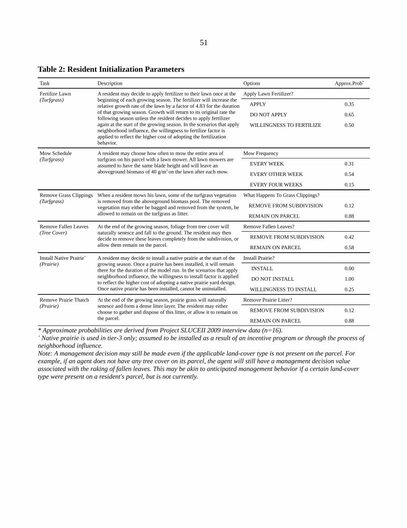
51
Table 2: Resident Initialization Parameters
Task Description Options Approx.Prob*
Fertilize Lawn(Turfgrass)
A resident may decide to apply fertilizer to their lawn once at the beginning of each growing season. The fertilizer will increase the relative growth rate of the lawn by a factor of 4.83 for the duration of that growing season. Growth will return to its original rate the following season unless the resident decides to apply fertilizer again at the start of the growing season. In the scenarios that apply neighborhood influence, the willingness to fertilize factor is applied to reflect the higher cost of adopting the fertilization behavior.
Apply Lawn Fertilizer?
APPLY 0.35
DO NOT APPLY 0.65
WILLINGNESS TO FERTILIZE 0.50
Mow Schedule(Turfgrass)
A resident may choose how often to mow the entire area of turfgrass on his parcel with a lawn mower. All lawn mowers are assumed to have the same blade height and will leave an aboveground biomass of 40 g/m2 on the lawn after each mow.
Mow Frequency
EVERY WEEK 0.31
EVERY OTHER WEEK 0.54
EVERY FOUR WEEKS 0.15
Remove Grass Clippings(Turfgrass)
When a resident mows his lawn, some of the turfgrass vegetation is removed from the aboveground biomass pool. The removed vegetation may either be bagged and removed from the system, be allowed to remain on the turfgrass as litter.
What Happens To Grass Clippings?
REMOVE FROM SUBDIVISION 0.12
REMAIN ON PARCEL 0.88
Remove Fallen Leaves(Tree Cover)
At the end of the growing season, foliage from tree cover will naturally senesce and fall to the ground. The resident may then decide to remove these leaves completely from the subdivision, or allow them remain on the parcel.
Remove Fallen Leaves?
REMOVE FROM SUBDIVISION 0.42
REMAIN ON PARCEL 0.58
Install Native Prairie+
(Prairie)A resident may decide to install a native prairie at the start of the growing season. Once a prairie has been installed, it will remain there for the duration of the model run. In the scenarios that apply neighborhood influence, the willingness to install factor is applied to reflect the higher cost of adopting a native prairie yard design. Once native prairie has been installed, cannot be uninstalled.
Install Prairie?
INSTALL 0.00
DO NOT INSTALL 1.00
WILLINGNESS TO INSTALL 0.25
Remove Prairie Thatch(Prairie)
At the end of the growing season, prairie grass will naturally senesce and form a dense litter layer. The resident may either choose to gather and dispose of this litter, or allow it to remain on the parcel.
Remove Prairie Litter?
REMOVE FROM SUBDIVISION 0.12
REMAIN ON PARCEL 0.88
* Approximate probabilities are derived from Project SLUCEII 2009 interview data (n=16).+ Native prairie is used in tier-3 only; assumed to be installed as a result of an incentive program or through the process of neighborhood influence. Note: A management decision may still be made even if the applicable land-cover type is not present on the parcel. For example, if an agent does not have any tree cover on its parcel, the agent will still have a management decision value associated with the raking of fallen leaves. This may be akin to anticipated management behavior if a certain land-cover type were present on a resident's parcel, but is not currently.
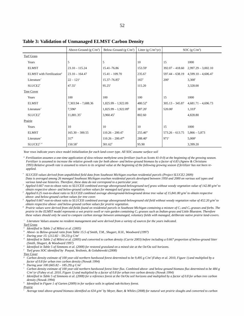
52
Table 3: Validation of Unmanaged ELMST Carbon Density
Above-Ground (g C/m2) Below-Ground (g C/m2) Litter (g C/m2/yr) SOC (g C/m2)
Turf Grass
Years 5 5 10 15 1000
ELMST 23.10 – 115.24 15.41–76.86 153.59c 392.07 – 418.60 2,997.29 – 3,002.10
ELMST with Fertilizationα 23.10 – 164.47 15.41 – 109.70 235.67 597.44 – 638.19 4,599.10 – 4,606.47
Literature+ 22 – 121a 15.37–76.85b 165d 200e 3,300f
SLUCE2* 47.551 95.251 115.20 3,328.00
Tree Cover
Years 100 100 100 15 1000
ELMST 7,303.94 – 7,688.36 1,825.99 – 1,922.09 480.52h 305.13 – 345.87 4,681.71 – 4,696.73
Literature+ 7,596g 1,825.99 – 1,922.09b 387.20i 520.00j 1,333k
SLUCE2* 11,881.352 3,960.452 802.60 4,828.80
Prairie
Years 10 10 10 15 1000
ELMST 165.30 – 300.55 110.26 – 200.47 255.46m 573.26 – 613.75 5,866 – 5,873
Literature+ 317l 110.26 – 200.47b 288.40n 971o 5,000p
SLUCE2*, 4 150.583 301.623 95.90 3,399.20
Year rows indicate years since model initialization for each land-cover type. All SOC assume surface soil
α Fertilization assumes a one-time application of slow-release methylene urea fertilizer (such as Scotts 41-0-0) at the beginning of the growing season. Fertilizer is assumed to increase the relative growth rate for both above- and below-ground biomass by a factor of 4.83 (Agnew & Christians 1993) Relative growth rate is assumed to return to its original value at the beginning of the following growing season if fertilizer has not been re-applied.
* SLUCEII values derived from unpublished field data from Southeast Michigan exurban residential parcels (Project SLUCE2 2009)Data is averaged among 26 managed Southeast Michigan exurban residential parcels developed between 1950 and 2000 on various soil types and various land-use histories. Therefore, these data do not correspond to a particular year.
1 Applied 0.667 root-to-shoot ratio to SLUCEII combined average aboveground-belowground turf grass without woody vegetation value of 142.80 g/m2 to obtain respective above- and below-ground carbon values for managed turf grass vegetation.
2 Applied 0.25 root-to-shoot ratio to SLUCEII combined average aboveground-belowground dense tree value of 15,841.80 g/m2 to obtain respective above- and below-ground carbon values for tree cover.
3 Applied 0.667 root-to-shoot ratio to SLUCEII combined average aboveground-belowground old field without woody vegetation value of 452.20 g/m2 to obtain respective above- and below-ground carbon values for prairie vegetation.
4 Prairie values were derived from old fields found on residential parcels in Southeast Michigan containing a mixture of C3 and C4 grasses and forbs. The prairie in the ELMST model represents a wet prairie swell or rain garden containing C4 grasses such as Indian-grass and Little Bluestem. Therefore these values should only be used to compare carbon storage between unmanaged, voluntary fields with managed, deliberate native prairie land-covers.
+ Literature Values assume no resident management and were derived from a variety of sources for the years indicated.Turf Grass a Identified in Table 2 of Milesi et al. (2005)b Above- to Below-ground ratio from Table 15.5 of Smith, T.M., Shugart, H.H., Woodward (1997)c During year 15: (212.82 – 59.23) g C/m2
d Identified in Table 2 of Milesi et al. (2005) and converted to carbon density (Currie 2003) before including a 0.667 proportion of below-ground litter (Smith, Shugart, & Woodward 1997)
e Identified in Table 5 of Simmons et al. (2008) for restored grassland on a mined site at the Oe/Oa soil horizons.f Turf grass SOC identified by Pouyat, Yesilonis, & Golubiewski (2008)Tree Coverg Carbon density estimate of 100 year-old northern hardwood forest determined to be 9,495 g C/m2 (Fahey et al. 2010, Figure 1) and multiplied by a
factor of 0.8 for urban tree carbon density (Nowak 1994)h During year 100 (665.82 – 185.29) g C/m2
i Carbon density estimate of 100 year-old northern hardwood forest litter flux. Combined above- and below-ground biomass flux determined to be 484 g C/m2/yr (Fahey et al. 2010, Figure 1) and multiplied by a factor of 0.8 for urban tree carbon density (Nowak 1994)
j Identified in Table 5 of Simmons et al. (2008) for a reference forest at the Oe/Oa soil horizons and multiplied by a factor of 0.8 for urban tree carbon density (Nowak 1994)
k Identified in Figure 1 of Garten (2009) in for surface soils in upland oak-hickory forest.Prairiel Average total above-ground biomass identified as 634 g/m2 by Meyer, Baer, & Whiles (2008) for natural wet prairie sloughs and converted to carbon
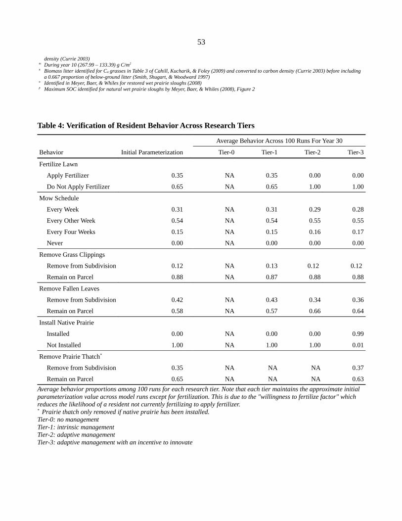
53
density (Currie 2003)m During year 10 (267.99 – 133.39) g C/m2
n Biomass litter identified for C4 grasses in Table 3 of Cahill, Kucharik, & Foley (2009) and converted to carbon density (Currie 2003) before including a 0.667 proportion of below-ground litter (Smith, Shugart, & Woodward 1997)
o Identified in Meyer, Baer, & Whiles for restored wet prairie sloughs (2008) p Maximum SOC identified for natural wet prairie sloughs by Meyer, Baer, & Whiles (2008), Figure 2
Table 4: Verification of Resident Behavior Across Research Tiers
Average Behavior Across 100 Runs For Year 30
Behavior Initial Parameterization Tier-0 Tier-1 Tier-2 Tier-3
Fertilize Lawn
Apply Fertilizer 0.35 NA 0.35 0.00 0.00
Do Not Apply Fertilizer 0.65 NA 0.65 1.00 1.00
Mow Schedule
Every Week 0.31 NA 0.31 0.29 0.28
Every Other Week 0.54 NA 0.54 0.55 0.55
Every Four Weeks 0.15 NA 0.15 0.16 0.17
Never 0.00 NA 0.00 0.00 0.00
Remove Grass Clippings
Remove from Subdivision 0.12 NA 0.13 0.12 0.12
Remain on Parcel 0.88 NA 0.87 0.88 0.88
Remove Fallen Leaves
Remove from Subdivision 0.42 NA 0.43 0.34 0.36
Remain on Parcel 0.58 NA 0.57 0.66 0.64
Install Native Prairie
Installed 0.00 NA 0.00 0.00 0.99
Not Installed 1.00 NA 1.00 1.00 0.01
Remove Prairie Thatch*
Remove from Subdivision 0.35 NA NA NA 0.37
Remain on Parcel 0.65 NA NA NA 0.63
Average behavior proportions among 100 runs for each research tier. Note that each tier maintains the approximate initial parameterization value across model runs except for fertilization. This is due to the "willingness to fertilize factor" which reduces the likelihood of a resident not currently fertilizing to apply fertilizer. * Prairie thatch only removed if native prairie has been installed.Tier-0: no managementTier-1: intrinsic managementTier-2: adaptive managementTier-3: adaptive management with an incentive to innovate
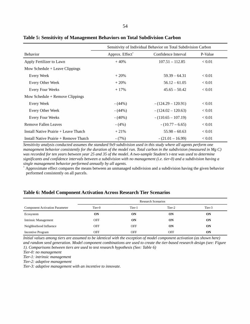
54
Table 5: Sensitivity of Management Behaviors on Total Subdivision Carbon
Sensitivity of Individual Behavior on Total Subdivision Carbon
Behavior Approx. Effect* Confidence Interval P-Value
Apply Fertilizer to Lawn + 40% 107.51 – 112.85 < 0.01
Mow Schedule + Leave Clippings
Every Week + 20% 59.39 – 64.31 < 0.01
Every Other Week + 20% 56.12 – 61.05 < 0.01
Every Four Weeks + 17% 45.65 – 50.42 < 0.01
Mow Schedule + Remove Clippings
Every Week - (44%) - (124.29 – 120.91) < 0.01
Every Other Week - (44%) - (124.02 – 120.63) < 0.01
Every Four Weeks - (40%) - (110.65 – 107.19) < 0.01
Remove Fallen Leaves - (4%) - (10.77 – 6.65) < 0.01
Install Native Prairie + Leave Thatch + 21% 55.98 – 60.63 < 0.01
Install Native Prairie + Remove Thatch - (7%) - (21.01 – 16.99) < 0.01
Sensitivity analysis conducted assumes the standard 9x9 subdivision used in this study where all agents perform one management behavior consistently for the duration of the model run. Total carbon in the subdivision (measured in Mg C) was recorded for ten years between year 25 and 35 of the model. A two-sample Student's t-test was used to determine significants and confidence intervals between a subdivision with no management (i.e. tier-0) and a subdivision having a single management behavior performed annually by all agents.* Approximate effect compares the means between an unmanaged subdivision and a subdivision having the given behavior
performed consistently on all parcels.
Table 6: Model Component Activation Across Research Tier Scenarios
Research Scenarios
Component Activation Parameter Tier-0 Tier-1 Tier-2 Tier-3
Ecosystem ON ON ON ON
Intrinsic Management OFF ON ON ON
Neighborhood Influence OFF OFF ON ON
Incentive Program OFF OFF OFF ON
Initial values among tiers are assumed to be identical with the exception of model component activation (as shown here) and random seed generation. Model component combinations are used to create the tier-based research design (see: Figure 1). Comparisons between tiers are used to test research hypothesis (See: Table 6) Tier-0: no managementTier-1: intrinsic managementTier-2: adaptive managementTier-3: adaptive management with an incentive to innovate.
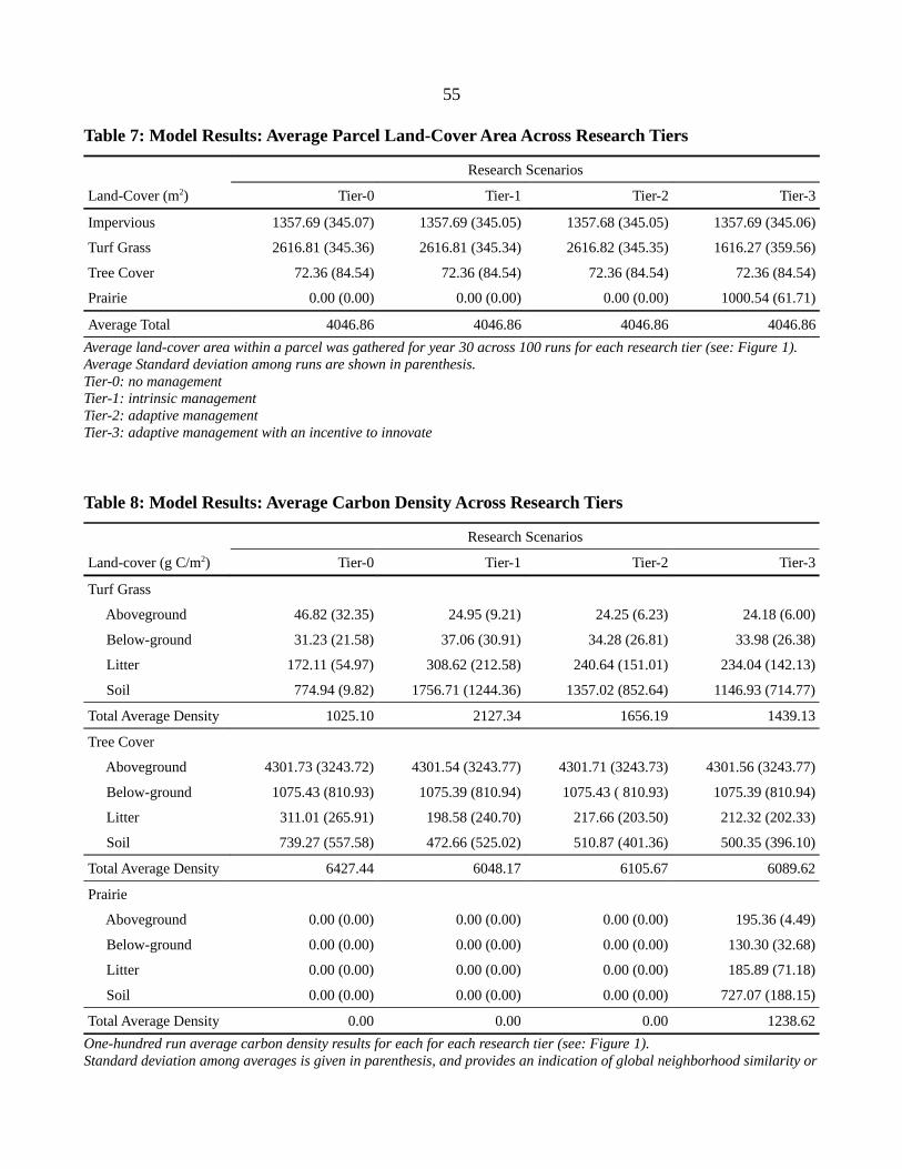
55
Table 7: Model Results: Average Parcel Land-Cover Area Across Research Tiers
Research Scenarios
Land-Cover (m2) Tier-0 Tier-1 Tier-2 Tier-3
Impervious 1357.69 (345.07) 1357.69 (345.05) 1357.68 (345.05) 1357.69 (345.06)
Turf Grass 2616.81 (345.36) 2616.81 (345.34) 2616.82 (345.35) 1616.27 (359.56)
Tree Cover 72.36 (84.54) 72.36 (84.54) 72.36 (84.54) 72.36 (84.54)
Prairie 0.00 (0.00) 0.00 (0.00) 0.00 (0.00) 1000.54 (61.71)
Average Total 4046.86 4046.86 4046.86 4046.86
Average land-cover area within a parcel was gathered for year 30 across 100 runs for each research tier (see: Figure 1). Average Standard deviation among runs are shown in parenthesis.Tier-0: no managementTier-1: intrinsic managementTier-2: adaptive managementTier-3: adaptive management with an incentive to innovate
Table 8: Model Results: Average Carbon Density Across Research Tiers
Research Scenarios
Land-cover (g C/m2) Tier-0 Tier-1 Tier-2 Tier-3
Turf Grass
Aboveground 46.82 (32.35) 24.95 (9.21) 24.25 (6.23) 24.18 (6.00)
Below-ground 31.23 (21.58) 37.06 (30.91) 34.28 (26.81) 33.98 (26.38)
Litter 172.11 (54.97) 308.62 (212.58) 240.64 (151.01) 234.04 (142.13)
Soil 774.94 (9.82) 1756.71 (1244.36) 1357.02 (852.64) 1146.93 (714.77)
Total Average Density 1025.10 2127.34 1656.19 1439.13
Tree Cover
Aboveground 4301.73 (3243.72) 4301.54 (3243.77) 4301.71 (3243.73) 4301.56 (3243.77)
Below-ground 1075.43 (810.93) 1075.39 (810.94) 1075.43 ( 810.93) 1075.39 (810.94)
Litter 311.01 (265.91) 198.58 (240.70) 217.66 (203.50) 212.32 (202.33)
Soil 739.27 (557.58) 472.66 (525.02) 510.87 (401.36) 500.35 (396.10)
Total Average Density 6427.44 6048.17 6105.67 6089.62
Prairie
Aboveground 0.00 (0.00) 0.00 (0.00) 0.00 (0.00) 195.36 (4.49)
Below-ground 0.00 (0.00) 0.00 (0.00) 0.00 (0.00) 130.30 (32.68)
Litter 0.00 (0.00) 0.00 (0.00) 0.00 (0.00) 185.89 (71.18)
Soil 0.00 (0.00) 0.00 (0.00) 0.00 (0.00) 727.07 (188.15)
Total Average Density 0.00 0.00 0.00 1238.62
One-hundred run average carbon density results for each for each research tier (see: Figure 1).Standard deviation among averages is given in parenthesis, and provides an indication of global neighborhood similarity or

56
cohesion.
Table 9: Model Results: Total Average Subdivision Carbon Across Tiers
Research Scenarios
Land-cover (Mg C) Tier-0 Tier-1 Tier-2 Tier-3
Turf Grass
Parcel Average 2.68 5.57 4.33 2.33
Subdivision Average 217.28 450.91 351.05 188.41
Tree Cover
Parcel Average 0.47 0.44 0.44 0.44
Subdivision Average 38.07 35.45 35.79 35.69
Prairie
Parcel Average 0.00 0.00 0.00 1.24
Subdivision Average 0.00 0.00 0.00 100.38
SUBDIVISION TOTAL AVERAGE 254.95 486.36 386.84 324.48
One-hundred run average total carbon results for each for each research tier (see: Figure 1).Parcel averages in Mg C were calculated by multiplying average land-cover area (Table 7) by average total carbon density (Table 8).Subdivision averages were calculated by multiplying the parcel average by the total number of parcels (i.e. 81).Subdivision total average is the sum of subdivision averages for each land-cover type.Tier-0: no managementTier-1: intrinsic managementTier-2: adaptive managementTier-3: adaptive management with an incentive to innovate
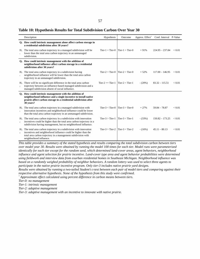
57
Table 10: Hypothesis Results for Total Subdivision Carbon Over Year 30
Description Hypothesis Outcome Approx. Effect* Conf. Interval P-Value
Q1 How could intrinsic management alone affect carbon storage in a residential subdivision after 30 years?
H1.
1
The total area carbon trajectory in a managed subdivision will be lower than the total area carbon trajectory in an unmanaged subdivision.
Tier-1 < Tier-0 Tier-1 > Tier-0 + 91% 224.95 – 237.84 < 0.01
Q2 How could intrinsic management with the addition of neighborhood influence affect carbon storage in a residential subdivision after 30 years?
H2.
1
The total area carbon trajectory in a subdivision having neighborhood influence will be lower than the total area carbon trajectory in an unmanaged subdivision.
Tier-2 < Tier-0 Tier-2 > Tier-0 + 52% 117.00 – 146.95 < 0.01
H2.
2
There will be no significant difference in the total area carbon trajectory between an influence-based managed subdivision and a managed subdivision absent of social influence.
Tier-2 == Tier-1 Tier-2 < Tier-1 - (20%) 83.32 – 115.51 < 0.01
Q3 How could intrinsic management with the addition of neighborhood influence and a single incentive to install native prairie affect carbon storage in a residential subdivision after 30 years?
H3.
1
The total area carbon trajectory in a managed subdivision with innovation incentives and neighborhood influence could be lower than the total area carbon trajectory in an unmanaged subdivision.
Tier-3 < Tier-0 Tier-3 > Tier-0 + 27% 59.84 – 78.87 < 0.01
H3.
2
The total area carbon trajectory in a subdivision with innovation incentives could be higher than the total area carbon trajectory in a subdivision having management, but no neighborhood influence.
Tier-3 > Tier-1 Tier-3 < Tier-1 - (33%) 150.82 – 173.25 < 0.01
H3.
3
The total area carbon trajectory in a subdivision with innovation incentives and neighborhood influence could be higher than the total area carbon trajectory in a management subdivision with neighborhood influence.
Tier-3 > Tier-2 Tier-3 < Tier-2 - (16%) 45.11 – 80.13 < 0.01
This table provides a summary of the stated hypothesis and results comparing the total subdivision carbon between tiers over model year 30. Results were obtained by running the model 100 times for each tier. Model runs were parameterized identically for each tier except for the random seed, which determined land-cover areas, agent behaviors, neighborhood influence and agent selection for prairie incentive. Land-cover type area and agent behavior probabilities were determined using fieldwork and interview data from exurban residential homes in Southeast Michigan. Neighborhood influence was based on a randomly weighed probability of neighbor behaviors. A random lottery was used to select three agents to participate in the native prairie incentive program. Only tier-3 includes native prairie yard designs. Results were obtained by running a two-tailed Student's t-test between each pair of model tiers and comparing against their respective alternative hypothesis. None of the hypothesis from this study were confirmed. * Approximate effect calculated using percent difference in carbon means between tiers.Tier-0: no managementTier-1: intrinsic managementTier-2: adaptive managementTier-3: adaptive management with an incentive to innovate with native prairie.

58
Table 11: Fieldwork: Eco-Zone Categories Translated to ELMST Land-Cover TypesEco-Zone Description Code Frequency Notes ELMST Land-Cover
Home/Building HO 26 Home or other buildings such as sheds and barns. Impervious
Pavement RP 26 Paved areas such as driveways, walkways and pools. Impervious
Shrubs with mulch and herbs CMSH 25 Gardens which are often times found around the periphery of a house and classified as impervious in areal photographs.
Impervious
Turf grass without woody vegetation CTG 25 Includes a mixture of C3 grasses and forbs. Turf Grass
Turf grass with sparse woody vegetation
CTGW 24 Includes a mixture of C3 grasses, forbs with a scattering of individual trees or shrubs.
Turf Grass
Vegetable garden CVG 8 Small, infrequent areas often times found within a CTG eco-zone and classified as turf grass on areal photographs.
Turf Grass
Water WA 4 Small pond on property. Turf Grass
Deciduous shrub CDS 1 Dense woody shrubs Tree Cover
Deciduous Tree CDT 5 Dense woody trees Tree Cover
Deciduous shrub and tree CDST 3 Dense woody shrubs and trees Tree Cover
Old field COF 4 Includes a mixture of C4 grasses, C3 grasses ans forbs. Prairie
Old Field with woody vegetation CFW 2 Includes a mixture of C4 grasses, C3 grasses, forbs and small clumps of deciduous shrubs or trees.
Prairie
Mapping of eco-zone categories from fieldwork data to ELMST land-cover types. Source: (Project SLUCE2 2009)
Table 12: Fieldwork: Land-Cover Areas for Parcels of One Acre or Less
Parcel ID Total Area (m 2 ) Proportion of Parcel Area
Impervious Turf Grass Tree Cover Prairie Total Impervious Turf Grass Tree Cover Prairie Total
R04 577.35 2642.28 0.00 0.00 3219.63 0.18 0.82 0.00 0.00 1.00
R06 423.71 1800.50 0.00 25.40 2249.61 0.19 0.80 0.00 0.01 1.00
R09 787.54 1246.88 0.00 0.00 2034.43 0.39 0.61 0.00 0.00 1.00
R10 838.17 2658.42 0.00 0.00 3496.59 0.24 0.76 0.00 0.00 1.00
R11 356.90 535.57 0.00 0.00 892.47 0.40 0.60 0.00 0.00 1.00
R12 732.45 1226.50 0.00 0.00 1958.95 0.37 0.63 0.00 0.00 1.00
R13 567.16 1050.17 0.00 0.00 1617.33 0.35 0.65 0.00 0.00 1.00
R15 836.57 1045.18 0.00 0.00 1881.75 0.44 0.56 0.00 0.00 1.00
R16 434.90 464.37 118.35 0.00 1017.62 0.43 0.46 0.12 0.00 1.00
R17 586.07 2203.64 0.00 0.00 2789.71 0.21 0.79 0.00 0.00 1.00
R18 341.77 1155.36 0.00 0.00 1497.13 0.23 0.77 0.00 0.00 1.00
R19 532.94 921.11 0.00 0.00 1454.05 0.37 0.63 0.00 0.00 1.00
R20 537.21 581.30 0.00 0.00 1118.51 0.48 0.52 0.00 0.00 1.00
R21 871.91 1410.21 0.00 0.00 2282.12 0.38 0.62 0.00 0.00 1.00
R22 505.45 431.48 0.00 31.30 968.24 0.52 0.45 0.00 0.03 1.00
R24 400.97 1396.03 0.00 0.00 1797.01 0.22 0.78 0.00 0.00 1.00
Mean 583.19 1298.06 7.40 3.54 1892.20 0.34 0.65 0.01 0.00 1.00
StdDev 178.46 711.29 29.59 9.74 778.70 0.11 0.12 0.03 0.00 0.00
Bold values used for initial model parameterization. Source: (Project SLUCE2 2009)
59
References
Aber, J.D., Melillo, J.M. & McClaugherty, C.A. (1990) Predicting long-term patterns of mass loss, nitrogen dynamics, and soil organic matter formation from initial fine litter chemistry in temperate forest ecosystems. Canadian Journal of Botany, 68, 2201-2208.
Agnew, M. & Christians, N. (1993) Influence of Fertilizer Source And Core Cultivation On The Growth of Kentucky Bluegrass. International Turfgrass Society Research Journal, 7, 458-463.
Akerlof, G.A. & Kranton, R.E. (2010) Identity economics: how our identities shape our work, wages, and well-being. Princeton University Press, Princeton, NJ.
An, L., Linderman, M., Qi, J., Shortridge, A. & Liu, J. (2005) Exploring Complexity in a Human-Environment System: An Agent-Based Spatial Model for Multidisciplinary and Multiscale Integration. Annals of the Association of American Geographers, 95, 54-79.
Axelrod, R. & Tesfatsion, L. (2010) On-Line Guide for Newcomers to Agent-Based Modeling in the Social Sciences. http://www2.econ.iastate.edu/tesfatsi/abmread.htm
Axelrod, R. (1997) The Dissemination of Culture: A Model with Local Convergence and Global Polarization. Journal of Conflict Resolution, 41, 203-226.
Bankes, S. (1993) Exploratory Modeling For Policy Analysis. Operations Research, 41, 435-449.
Barabasi, A. (2003) Linked: How Everything is Connected to Everything Else and What it Means. Plume, New York, New York, USA.
Benson, B.S. & Surles, T. (2006) Carbon Dioxide Capture and Storage : An Overview With Emphasis on Capture and Storage in Deep Geological Formations. Proceedings of the IEEE.
Bishop, B. (2008) The Big Sort. Houghton Mifflin Harcourt, New York.
Blackman, V. (1919) The Compound Interest Law and Plant Growth. Annuals of Botany, 33.
Bowman, T. & Thompson, J. (2009) Barriers to implementation of low-impact and conservation subdivision design: Developer perceptions and resident demand. Landscape and Urban Planning, 92, 96-105.
Brown, D.G. & Robinson, D.T. (2006) Effects of Heterogeneity in Residential Preferences on an Agent-Based Model of Urban Sprawl. Ecology And Society, 11.
Brown, D.G., Johnson, K.M., Loveland, T.R. & Theobald, D.M. (2005) Rural Land-Use Trends in the Conterminous United States, 1950–2000. Ecological Applications, 15, 1851-1863.
Brown, D.G., Robinson, D.T., An, L., Nassauer, J.I., Zellner, M., Rand, W., Riolo, R., Page, S.E., Low, B. & Wang, Z. (2008) Exurbia from the bottom-up: Confronting empirical challenges to characterizing a complex system. Geoforum, 39, 805-818.
Burchell, R.W., Downs, A., McCann, B. & Mukherji, S. (2005) Sprawl Costs: Economic Impacts of

60
Unchecked Development. Island Press, Washington, DC.
Cahill, K.N., Kucharik, C.J. & Foley, J.A. (2009) Prairie restoration and carbon sequestration: difficulties quantifying C sources and sinks using a biometric approach. Ecological Applications, 19, 2185-201.
Centola, D., Willer, R. & Macy, M. (2005) The Emperor’s Dilemma: A Computational Model of Self‐Enforcing Norms. American Journal of Sociology, 110, 1009-1040.
Christakis, N.A. & Fowler, J.H. (2009) Connected: The Surprising Power of Our Social Networks and How They Shape Our Lives. Little, Brown and Company, New York, New York, USA.
Christakis, N.a. & Fowler, J.H. (2007) The spread of obesity in a large social network over 32 years. The New England Journal of Medicine, 357, 370-9.
Cioffi-Revilla, C. (2010) A Methodology for Complex Social Simulations. Journal of Artificial Societies and Social Simulation, 13.
Cook, W.M., Casagrande, D.G., Hope, D., Groffman, P.M., L, S. & Collins, S.L. (2004) Learning to Roll with the Punches: Adaptive Experimentation in Human-Dominated Systems. Frontiers in Ecology and the Environment, 2, 467-474.
Currie, W.S. & Aber, J.D. (1997) Modeling Leaching As a Decomposition Process in Humid Montane Forests. Ecology, 78, 1844-1860.
Currie, W.S., Harmon, M.E., Burke, I.C., Hart, S.C., Parton, W.J. & Silver, W. (2009) Cross-biome transplants of plant litter show decomposition models extend to a broader climatic range but lose predictability at the decadal time scale. Global Change Biology, 16, 1744-1761.
Currie, W.S. (2003) Relationships between carbon turnover and bioavailable energy fluxes in two temperate forest soils. Global Change Biology, 9, 919-929.
Damgaard, C. (2004) Modelling individual plant growth at a variable mean density or at a specific spatial setting. Comptes Rendus Biologies, 327, 255-260.
Damgaard, C. Richards growth model. Ecology, 1-3.
Dixon, David S., Reynolds, W.N. On Quantitative Models for Qualitative Data: Case Studies in Agent-Based Socio-polictical Modeling. Acta Sociologica.
Dixon, R.K., Solomon, A.M., Brown, S., Houghton, R.A., Trexier, M.C. & Wisniewski, J. (1994) Carbon pools and flux of global forest ecosystems. Science, 263, 185-90.
Eclipse. (2000) Eclipse Integrated Development Environment, v.3.5. Eclipse Foundation.
Ellis, E.C. & Ramankutty, N. (2008) Putting people in the map: anthropogenic biomes of the world. Frontiers in Ecology and the Environment, 6, 439-447.
Epstein, J.M. (2008) Why Model? Journal of Artificial Societies and Social Simulation, 11, 12.

61
Fahey, T.J., Woodbury, P.B., Battles, J.J., Goodale, C.L., Hamburg, S., Ollinger, S. & Woodall, C.W. (2010) Forest carbon storage: ecology, management, and policy. Frontiers in Ecology and the Environment, 8, 245-252.
Galster, G.C. (1987) Homeowners and Neighborhood Reinvestment. Duke University Press, Durham, NC.
Grimm, V. & Railsback, S.F. (2005) Individual-based Modeling and Ecology. Princeton University Press, Princeton, NJ.
Grimm, V., Berger, U., Bastiansen, F., Eliassen, S., Ginot, V., Giske, J., Goss-Custard, J., Grand, T., Heinz, S.K. & Huse, G. (2006) A standard protocol for describing individual-based and agent-based models. Ecological Modelling, 198, 115-126.
Génard, M., Pagès, L. & Kervella, J. (1998) A carbon balance model of peach tree growth and development for studying the pruning response. Tree physiology, 18, 351-362.
Houghton, R., Hackler, J. & Lawrence, K. (1999) The U.S. Carbon budget: contributions from land-Use change. Science, 285, 574-8.
Hutnik Russell J., Yawney, H.W. (1961) Silvical Characteristics of Red Maple. Upper Darby, PA.
IPCC. (2000) Land Use, Land-Use Change and Forestry.Watson, Robert T., Noble, Ian R., Bolin Bert, Ravindranath, N. H., Verardo, David J., Dokken, D.J., Cambridge University Press, UK.
Ioannides, Y.M. (2002) Residential neighborhood effects. Regional Science and Urban Economics, 32, 145-165.
Java. (2002) Java 2 Platform, Enterprise Edition SDK. Oracle.
Kaye, J.P., Groffman, P.M., Grimm, N.B., Baker, L.A. & Pouyat, R.V. (2006) A distinct urban biogeochemistry? Trends in Ecology & Evolution, 21, 192-9.
Kucharik, C.J., Brye, K.R., Norman, J.M., Foley, J.A., Gower, S.T. & Bundy, L.G. (2001) Measurements and Modeling of Carbon and Nitrogen Cycling in Agroecosystems of Southern Wisconsin : Potential for SOC Sequestration during the Next 50 Years. Ecosystems, 4, 237-258.
Lesch, L. (2010) Strategies for Enhancing Carbon Sequestration and Co-Benevits in Human Dominated Landscapes. MS Thesis. School of Natural Resources and Environment. University of Michigan. Ann Arbor, MI. USA.
Levang-brilz, N. & Biondini, M.E. (2002) Growth rate , root development and nutrient uptake of 55 plant species from the Great Plains Grasslands , USA. Plant Ecology, 165, 117-144.
Liu, J., Dietz, T., Carpenter, S.R., Folke, C., Alberti, M., Redman, C.L., Schneider, S.H., Ostrom, E., Pell, A.N., Lubchenco, J., Taylor, W.W., Ouyang, Z., Deadman, P., Kratz, T. & Provencher, W. (2007) Coupled human and natural systems. Ambio, 36, 639-49.
Mason, W.a., Conrey, F.R. & Smith, E.R. (2007) Situating social influence processes: dynamic,
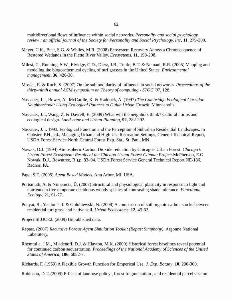
62
multidirectional flows of influence within social networks. Personality and social psychology review : an official journal of the Society for Personality and Social Psychology, Inc, 11, 279-300.
Meyer, C.K., Baer, S.G. & Whiles, M.R. (2008) Ecosystem Recovery Across a Chronosequence of Restored Wetlands in the Platte River Valley. Ecosystems, 11, 193-208.
Milesi, C., Running, S.W., Elvidge, C.D., Dietz, J.B., Tuttle, B.T. & Nemani, R.R. (2005) Mapping and modeling the biogeochemical cycling of turf grasses in the United States. Environmental management, 36, 426-38.
Mossel, E. & Roch, S. (2007) On the submodularity of influence in social networks. Proceedings of the thirty-ninth annual ACM symposium on Theory of computing - STOC '07, 128.
Nassauer, J.I., Bower, A., McCardle, K. & Kaddock, A. (1997) The Cambridge Ecological Corridor Neighborhood: Using Ecological Patterns to Guide Urban Growth. Minneapolis.
Nassauer, J.I., Wang, Z. & Dayrell, E. (2009) What will the neighbors think? Cultural norms and ecological design. Landscape and Urban Planning, 92, 282-292.
Nassauer, J. I. 1993. Ecological Function and the Perception of Suburban Residential Landscapes. In Gobster, P.H., ed., Managing Urban and High Use Recreation Settings, General Technical Report, USDA Forest Service North Central Forest Exp. Sta., St. Paul, MN.
Nowak, D.J. (1994) Atmospheric Carbon Dioxide reduction by Chicago's Urban Forest. Chicago’s Urban Forest Ecosystem: Results of the Chicago Urban Forest Climate Project.McPherson, E.G., Nowak, D.J., Rowntree, R.),p. 83–94. USDA Forest Service General Technical Report NE-186, Radnor, PA.
Page, S.E. (2005) Agent Based Models. Ann Arbor, MI. USA.
Portsmuth, A. & Niinemets, Ü. (2007) Structural and physiological plasticity in response to light and nutrients in five temperate deciduous woody species of contrasting shade tolerance. Functional Ecology, 21, 61-77.
Pouyat, R., Yesilonis, I. & Golubiewski, N. (2008) A comparison of soil organic carbon stocks between residential turf grass and native soil. Urban Ecosystems, 12, 45-62.
Project SLUCE2. (2009) Unpublished data.
Repast. (2007) Recursive Porous Agent Simulation Toolkit (Repast Simphony). Argonne National Laboratory.
Rhemtulla, J.M., Mladenoff, D.J. & Clayton, M.K. (2009) Historical forest baselines reveal potential for continued carbon sequestration. Proceedings of the National Academy of Sciences of the United States of America, 106, 6082-7.
Richards, F. (1959) A Flexible Growth Function for Emperical Use. J. Exp. Botany, 10, 290-300.
Robinson, D.T. (2009) Effects of land-use policy , forest fragmentation , and residential parcel size on
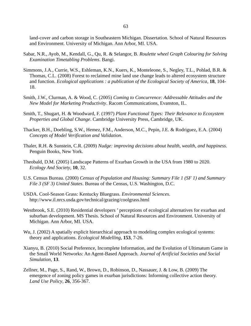
63
land-cover and carbon storage in Southeastern Michigan. Dissertation. School of Natural Resources and Environment. University of Michigan. Ann Arbor, MI. USA.
Sabar, N.R., Ayob, M., Kendall, G., Qu, R. & Selangor, B. Roulette wheel Graph Colouring for Solving Examination Timetabling Problems. Bangi.
Simmons, J.A., Currie, W.S., Eshleman, K.N., Kuers, K., Monteleone, S., Negley, T.L., Pohlad, B.R. & Thomas, C.L. (2008) Forest to reclaimed mine land use change leads to altered ecosystem structure and function. Ecological applications : a publication of the Ecological Society of America, 18, 104-18.
Smith, J.W., Clurman, A. & Wood, C. (2005) Coming to Concurrence: Addressable Attitudes and the New Model for Marketing Productivity. Racom Communications, Evanston, IL.
Smith, T., Shugart, H. & Woodward, F. (1997) Plant Functional Types: Their Relevance to Ecosystem Properties and Global Change. Cambridge University Press, Cambridge, UK.
Thacker, B.H., Doebling, S.W., Hemez, F.M., Anderson, M.C., Pepin, J.E. & Rodriguez, E.A. (2004) Concepts of Model Verification and Validation.
Thaler, R.H. & Sunstein, C.R. (2009) Nudge: improving decisions about health, wealth, and happiness. Penguin Books, New York.
Theobald, D.M. (2005) Landscape Patterns of Exurban Growth in the USA from 1980 to 2020. Ecology And Society, 10, 32.
U.S. Census Bureau. (2000) Census of Population and Housing: Summary File 1 (SF 1) and Summary File 3 (SF 3) United States. Bureau of the Census, U.S. Washington, D.C.
USDA. Cool-Season Grass: Kentucky Bluegrass. Environmental Sciences. http://www.il.nrcs.usda.gov/technical/grazing/coolgrass.html
Westbrook, S.E. (2010) Residential developers ’ perceptions of ecological alternatives for exurban and suburban development. MS Thesis. School of Natural Resources and Environment. University of Michigan. Ann Arbor, MI. USA.
Wu, J. (2002) A spatially explicit hierarchical approach to modeling complex ecological systems: theory and applications. Ecological Modelling, 153, 7-26.
Xianyu, B. (2010) Social Preference, Incomplete Information, and the Evolution of Ultimatum Game in the Small World Networks: An Agent-Based Approach. Journal of Artificial Societies and Social Simulation, 13.
Zellner, M., Page, S., Rand, W., Brown, D., Robinson, D., Nassauer, J. & Low, B. (2009) The emergence of zoning policy games in exurban jurisdictions: Informing collective action theory. Land Use Policy, 26, 356-367.
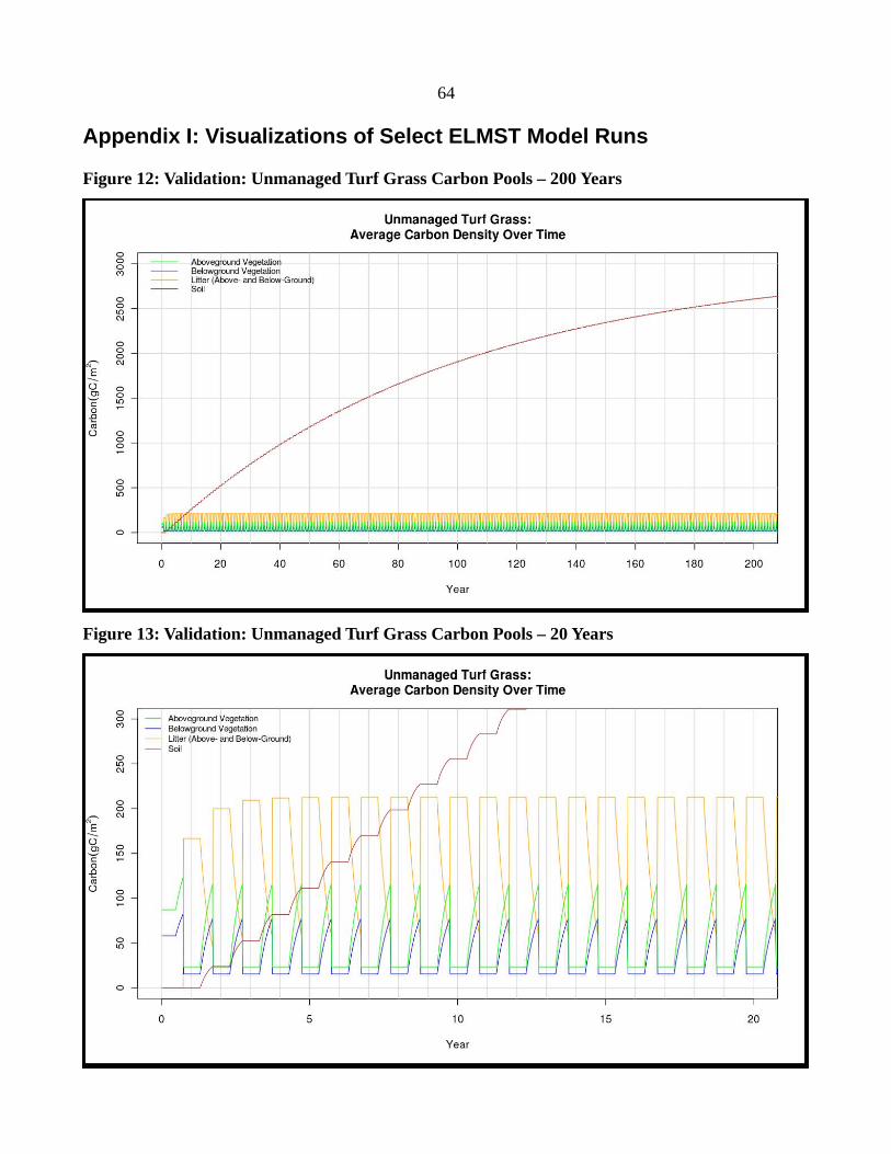
64
Appendix I: Visualizations of Select ELMST Model Runs
Figure 12: Validation: Unmanaged Turf Grass Carbon Pools – 200 Years
Figure 13: Validation: Unmanaged Turf Grass Carbon Pools – 20 Years
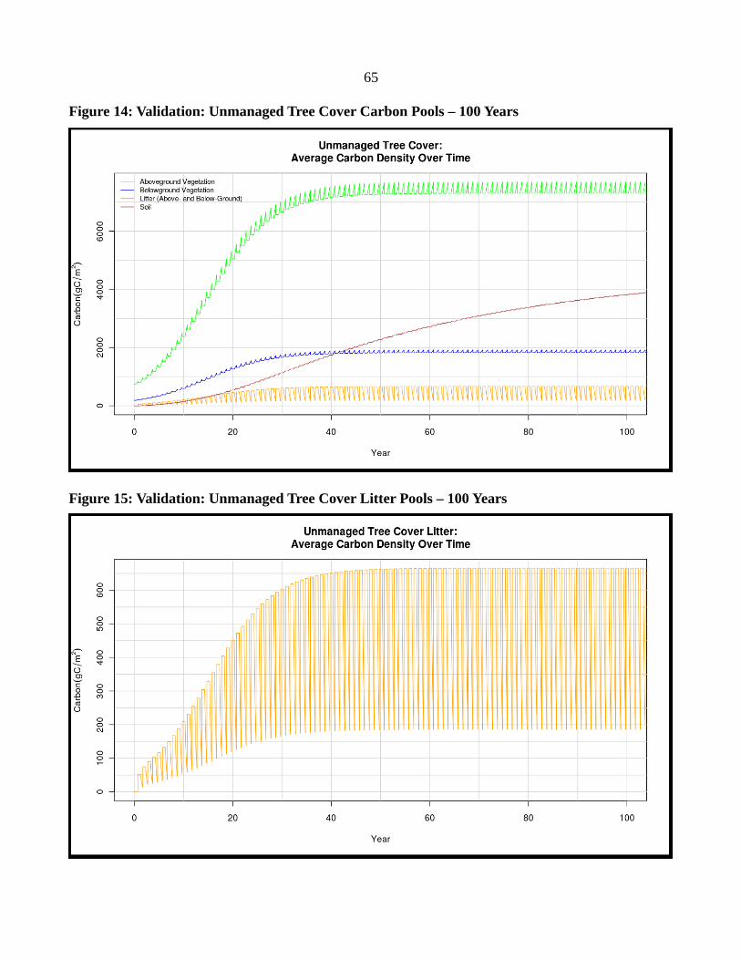
65
Figure 14: Validation: Unmanaged Tree Cover Carbon Pools – 100 Years
Figure 15: Validation: Unmanaged Tree Cover Litter Pools – 100 Years
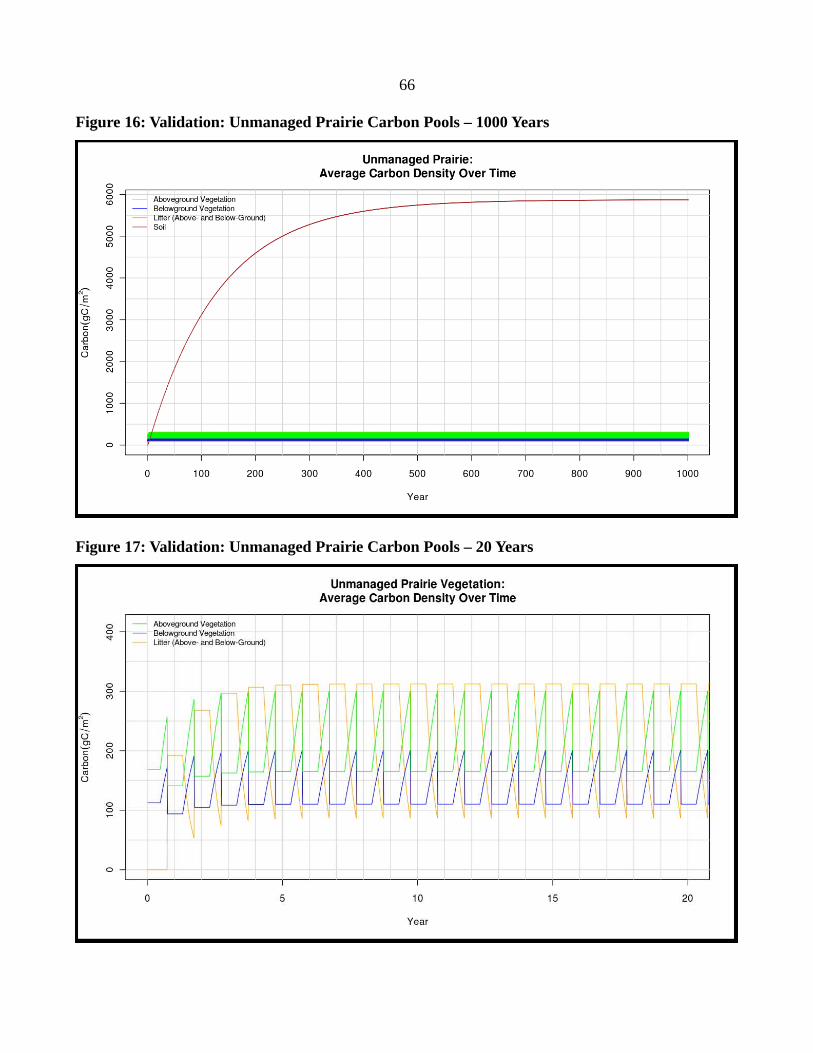
66
Figure 16: Validation: Unmanaged Prairie Carbon Pools – 1000 Years
Figure 17: Validation: Unmanaged Prairie Carbon Pools – 20 Years
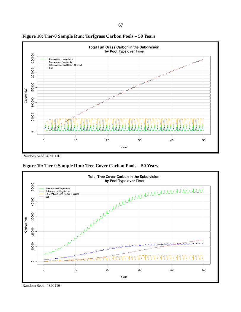
67
Figure 18: Tier-0 Sample Run: Turfgrass Carbon Pools – 50 Years
Random Seed: 4390116
Figure 19: Tier-0 Sample Run: Tree Cover Carbon Pools – 50 Years
Random Seed: 4390116
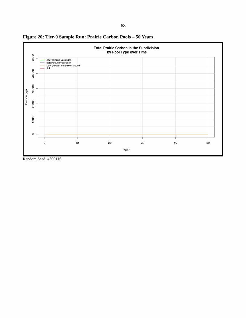
68
Figure 20: Tier-0 Sample Run: Prairie Carbon Pools – 50 Years
Random Seed: 4390116
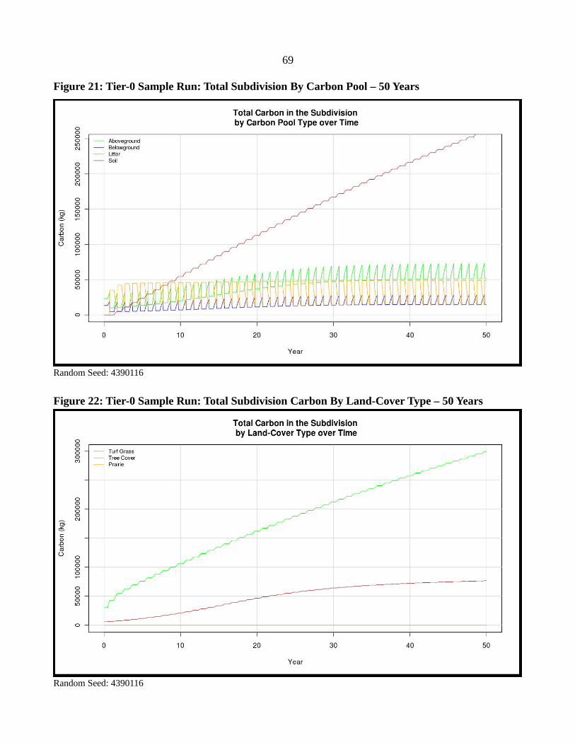
69
Figure 21: Tier-0 Sample Run: Total Subdivision By Carbon Pool – 50 Years
Random Seed: 4390116
Figure 22: Tier-0 Sample Run: Total Subdivision Carbon By Land-Cover Type – 50 Years
Random Seed: 4390116
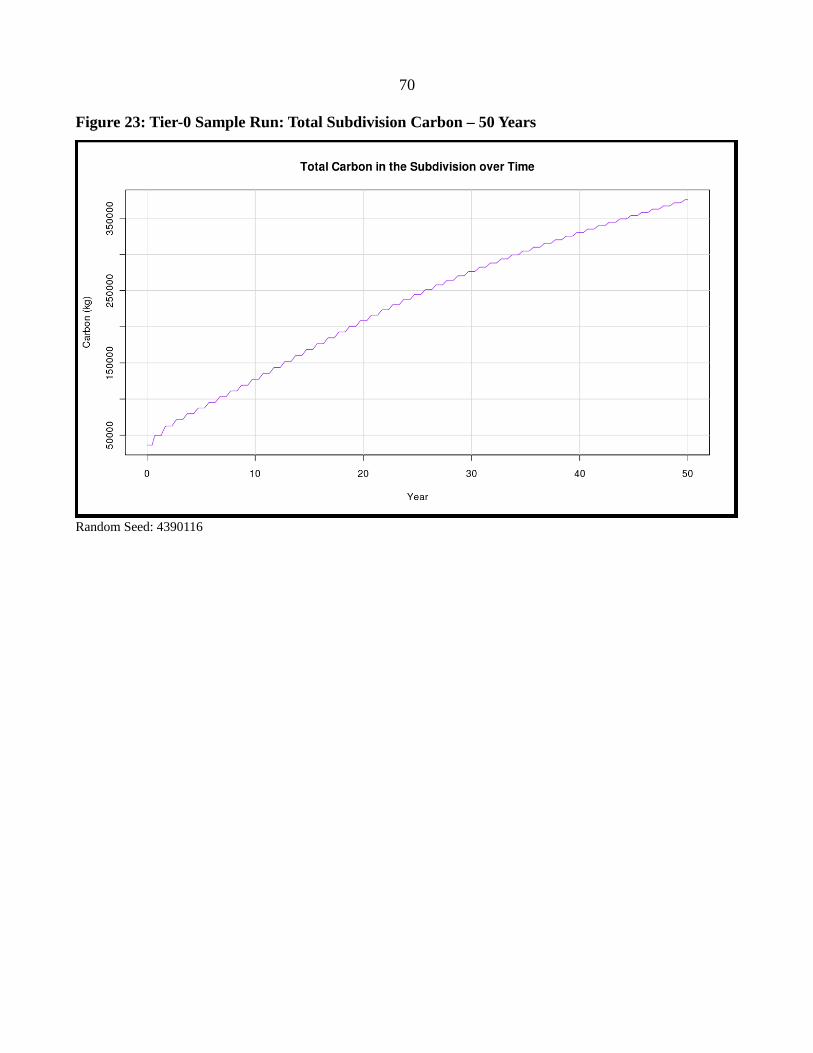
70
Figure 23: Tier-0 Sample Run: Total Subdivision Carbon – 50 Years
Random Seed: 4390116

71
Figure 24: Tier-1 Sample Run: Proportion of Resident Behaviors – 30 Years
Random Seed: 4390116
Figure 25: Tier-1 Sample Run: Proportion of Lawn Mowing Schedules – 30 Years
Random Seed: 4390116
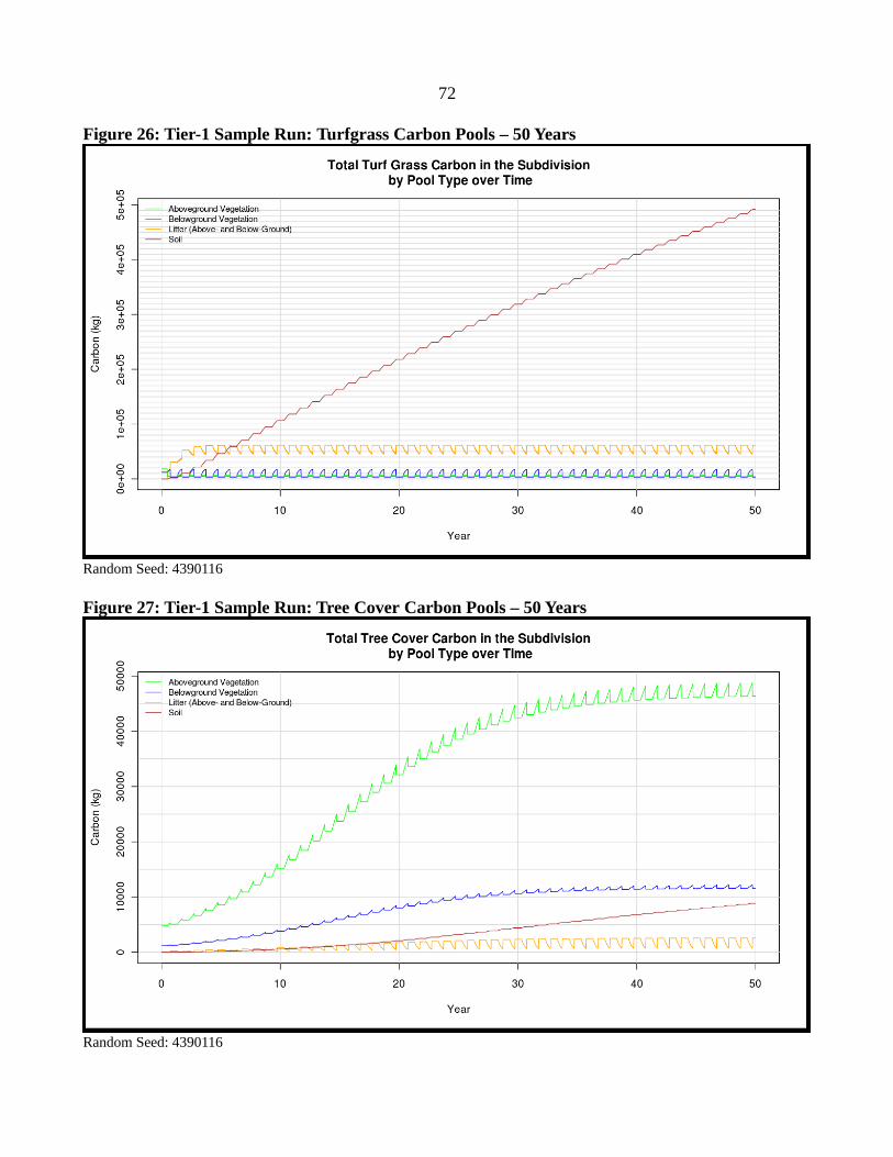
72
Figure 26: Tier-1 Sample Run: Turfgrass Carbon Pools – 50 Years
Random Seed: 4390116
Figure 27: Tier-1 Sample Run: Tree Cover Carbon Pools – 50 Years
Random Seed: 4390116
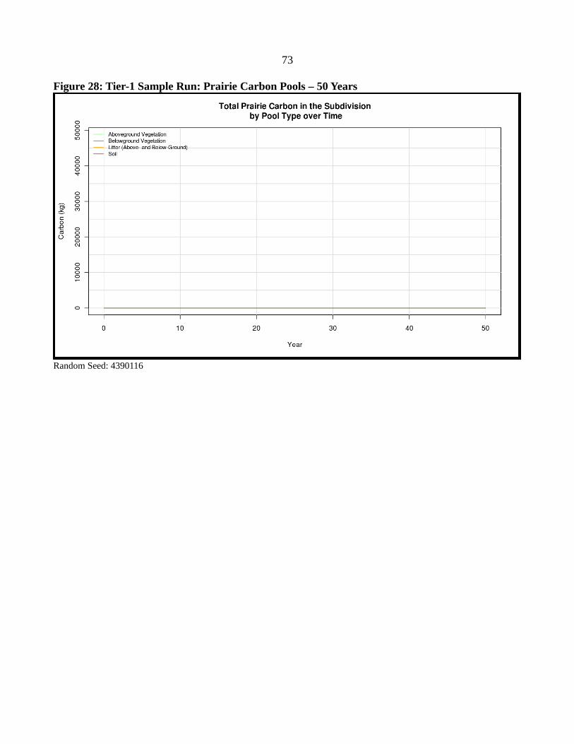
73
Figure 28: Tier-1 Sample Run: Prairie Carbon Pools – 50 Years
Random Seed: 4390116
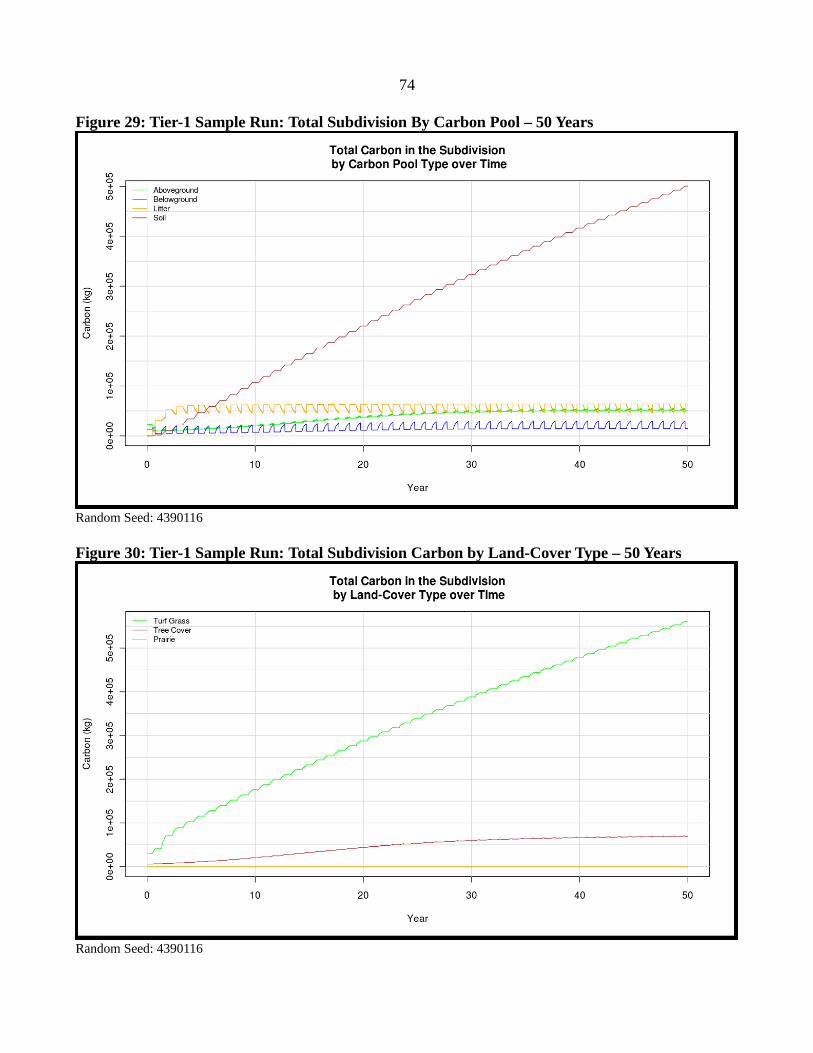
74
Figure 29: Tier-1 Sample Run: Total Subdivision By Carbon Pool – 50 Years
Random Seed: 4390116
Figure 30: Tier-1 Sample Run: Total Subdivision Carbon by Land-Cover Type – 50 Years
Random Seed: 4390116
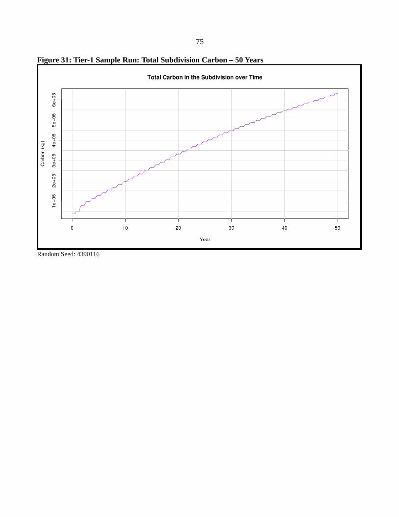
75
Figure 31: Tier-1 Sample Run: Total Subdivision Carbon – 50 Years
Random Seed: 4390116

76
Figure 32: Tier-2 Sample Run: Proportion of Resident Behaviors – 30 Years
Random Seed: 4390116
Figure 33: Tier-2 Sample Run: Proportion of Lawn Mowing Schedules – 30 Years
Random Seed: 4390116

77
Figure 34: Tier-2 Sample Run: Turfgrass Carbon Pools – 50 Years
Random Seed: 4390116
Figure 35: Tier-2 Sample Run: Tree Cover Carbon Pools – 50 Years
Random Seed: 4390116

78
Figure 36: Tier-1 Sample Run: Prairie Carbon Pools – 50 Years
Random Seed: 4390116

79
Figure 37: Tier-2 Sample Run: Total Subdivision Carbon by Carbon Pool – 50 Years
Random Seed: 4390116
Figure 38: Tier-2 Sample Run: Total Subdivision Carbon by Land-Cover Type – 50 Years
Random Seed: 4390116
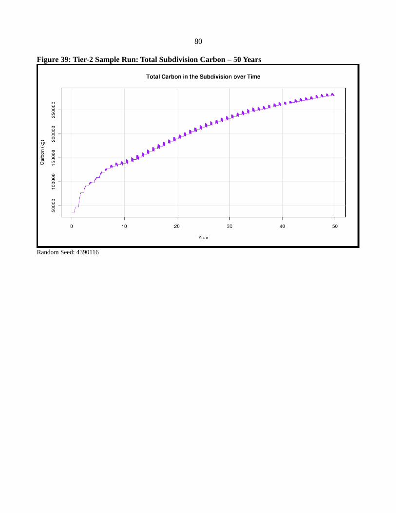
80
Figure 39: Tier-2 Sample Run: Total Subdivision Carbon – 50 Years
Random Seed: 4390116
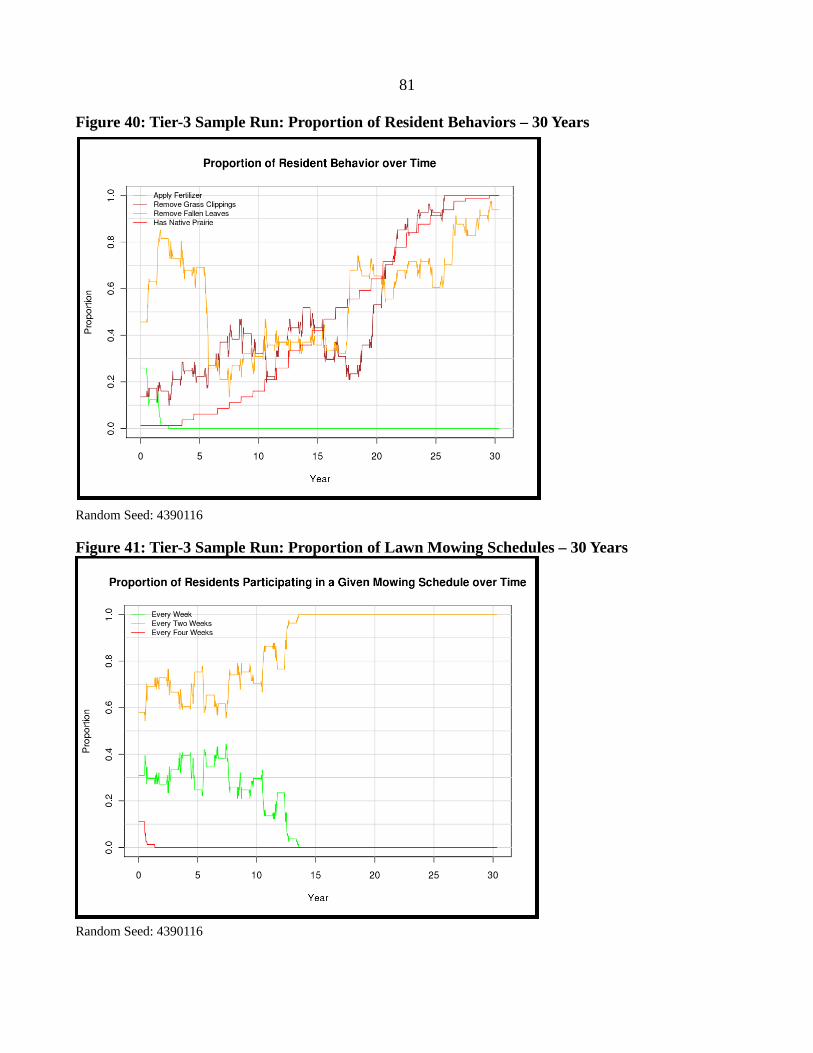
81
Figure 40: Tier-3 Sample Run: Proportion of Resident Behaviors – 30 Years
Random Seed: 4390116
Figure 41: Tier-3 Sample Run: Proportion of Lawn Mowing Schedules – 30 Years
Random Seed: 4390116
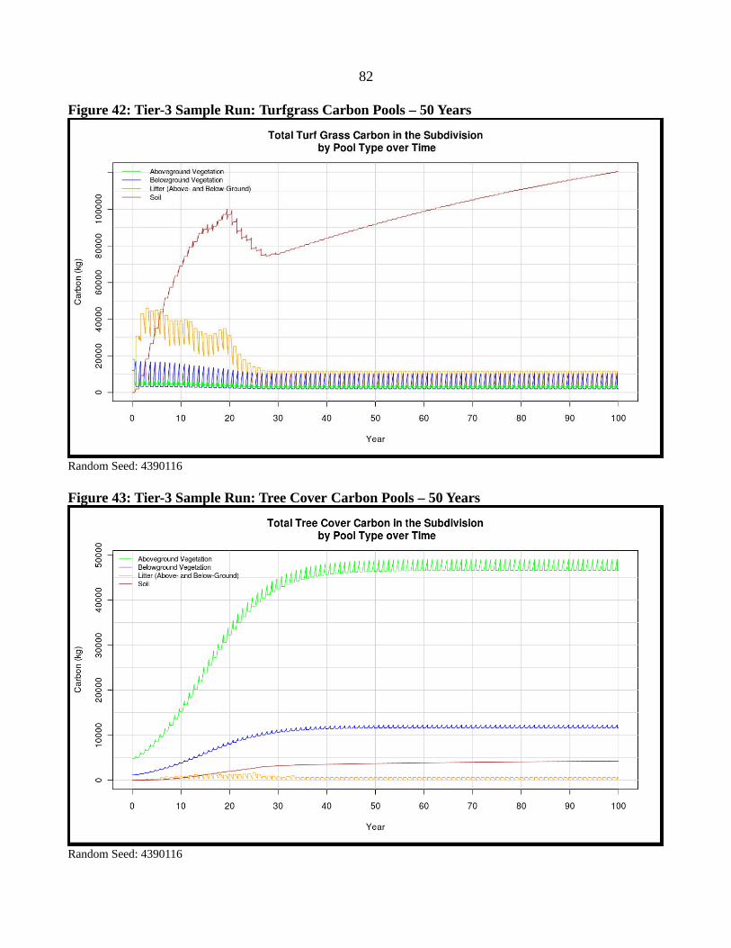
82
Figure 42: Tier-3 Sample Run: Turfgrass Carbon Pools – 50 Years
Random Seed: 4390116
Figure 43: Tier-3 Sample Run: Tree Cover Carbon Pools – 50 Years
Random Seed: 4390116
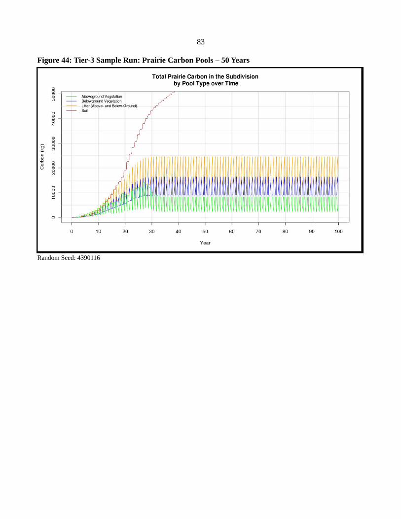
83
Figure 44: Tier-3 Sample Run: Prairie Carbon Pools – 50 Years
Random Seed: 4390116
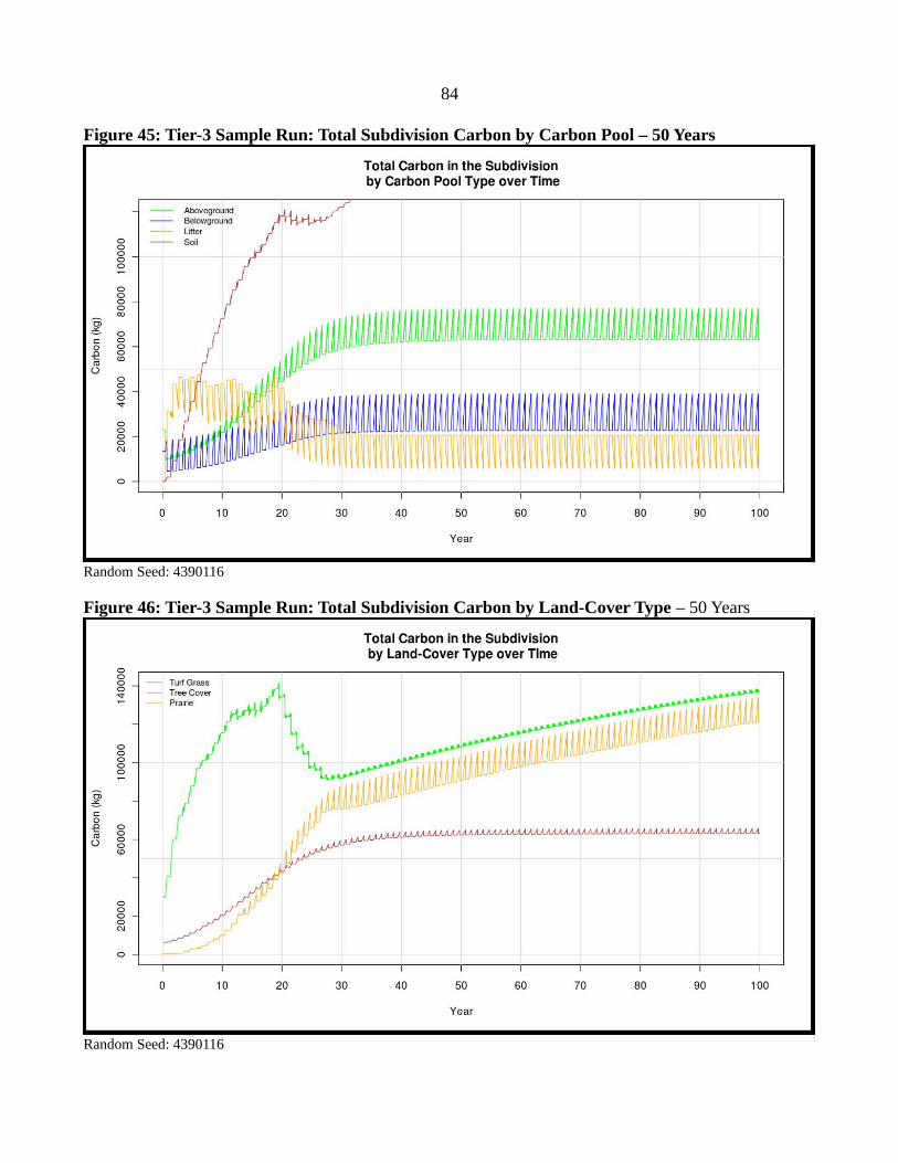
84
Figure 45: Tier-3 Sample Run: Total Subdivision Carbon by Carbon Pool – 50 Years
Random Seed: 4390116
Figure 46: Tier-3 Sample Run: Total Subdivision Carbon by Land-Cover Type – 50 Years
Random Seed: 4390116

85
Figure 47: Tier-3 Sample Run: Total Subdivision Carbon – 50 Years
Random Seed: 4390116