exploring the relationship between socio-economic ... · exploring the relationship between...

Exploring the relationship between socio-economic inequality, political instability and economic growthWhy do we know so little?

Gunhild Gram Giskemo

WP 2012: 2

Chr. Michelsen Institute (CMI) is an independent, non-profit research institution and a major international centre in policy-oriented and applied development research. Focus is on development and human rights issues and on international conditions that affect such issues. The geographical focus is Sub-Saharan Africa, Southern and Central Asia, the Middle East and Latin America.

CMI combines applied and theoretical research. CMI research intends to assist policy formulation, improve the basis for decision-making and promote public debate on international development issues.

Exploring the relationship between socio-economic inequality, political instability

and economic growth

Why do we know so little?

Gunhild Gram Giskemo

WP 2012: 2

CMI WORKING PAPER EXPLORING THE RELATIONSHIP BETWEEN SOCIO-ECONOMIC INEQUALITY, POLITICAL INSTABILITY AND ECONOMIC GROWTH

WP 2012:2

3

Contents Abstract ........................................................................................................................................................... 4

1. Introduction ............................................................................................................................................ 5

1.1 The effect of inequality on political instability ...................................................................................... 5 1.2 The effect of political instability on economic growth .......................................................................... 7

2. Methodology and measurement ............................................................................................................. 8

2.1 Measuring socio-economic inequality ................................................................................................. 10 2.2 Measuring political instability .............................................................................................................. 11 2.3 Measuring economic development ..................................................................................................... 11 2.4 The control variables ........................................................................................................................... 12

3. Results .................................................................................................................................................. 14

3.1 EQUATION 1: Political instability as the dependent variable .............................................................. 15 3.2 EQUATION 2: Economic development as the dependent variable ...................................................... 17

4. Discussion ............................................................................................................................................. 19

4.1 The robustness of the different measures .......................................................................................... 19 4.2 Differences between the recursive and the S.E. models ..................................................................... 21 4.3 Possible critiques of the methods used in the analysis ....................................................................... 22

5. Conclusive remarks ............................................................................................................................... 23

Bibliography ................................................................................................................................................... 24

APPENDIX A: Detailed variable description .................................................................................................... 28

APPENDIX B: Descriptive statistics ................................................................................................................. 31


WP 2012:2

4

Abstract The hypothesis that socio-economic inequality has a detrimental effect on economic growth by breeding political instability has been subject to empirical investigation for decades. However, the numerous studies in the field have yielded highly different conclusions, and still no agreement has been reached as to what the relationship between these variables really looks like. This study investigates why empirical studies have given such diverging results. By using several different measures both of socio-economic inequality, political instability and economic development it examines whether differences in methods and measurement can explain the variation in previous findings. It is revealed that the effect of socio-economic inequality upon political instability is dependent on which measures are used, and that the effect of instability upon economic development varies between different analytical models. The study thus shows that conclusions about the relationship between these phenomena are not robust to alternative measurement. A possible explanation of why previous empirical studies have reported such diverging findings is therefore that socio-economic inequality and political instability have been measured in different ways, or that different analytical models have been used.1

1 The paper is based upon the author’s master thesis on the subject (Giskemo 2008: https://bora.uib.no/handle/1956/5381). Details on the theoretical basis, methodology, measurement and analytical results can be found here.

https://bora.uib.no/handle/1956/5381�


WP 2012:2

5

1. Introduction Does socio-economic inequality reduce the rate of economic development? Despite the long-lasting academic interest in the subject (Galor and Zeira 1993), still no agreement has been reached as to whether the effect of inequality upon economic growth really is negative, and the divergence in both theoretical expectations and empirical findings has spurred a continued interest in the subject (MacCulloch 2005). Contrary to the conventional wisdom that socio-economic inequality is good for growth,2

1.1 The effect of inequality on political instability

the majority of the studies pertaining to the so-called “new growth wave” of the 1990s claim to show that the relationship is actually negative (e.g. Benabou 1996; Tanninen 1999; and Clarke 1995). However, such reduced form analyses are not very enlightening when it comes to explaining the specific determinants through which inequality affects growth (Bandyopadhyay and Basu 2005). Several studies thus explore various paths of causation between these two phenomena (Castello and Domenech 2002). One of these paths is the hypothesis that socio-economic inequality reduces economic growth by breeding political instability. This alleged causal pattern has been subject to academic focus and empirical investigations since the times of the Ancient Greeks (Lichbach (1989). What theoretical expectations lie behind the hypothesis?

A remarkably diverse literature, ancient and modern, ideological and theoretical, has coalesced on the assertion that political violence is a function of economic inequality (Sigelman and Simpson 1977).3 A highly unequal, polarised distribution of resources is thought to produce relative deprivation and in that way being an important source of discontent (Gurr (1970).4

A large group of impoverished citizens, facing a small and very rich group of well-off individuals is likely to become dissatisfied with the existing socio-economic status quo and demand radical changes, so that mass violence and illegal seizure of power are more likely than, when income distribution is more equitable.

In that way, a high degree of inequality creates incentives to engage in violent protests, coups or other politically destabilising activities (Festinger 1954; Muller 1985; Lichbach 1989; Schock 1996). Alesina and Perotti (1996: 1214) describe this causal relationship in their seminal work “Income distribution, political instability and investment”:

When comparing different paths of causation, Perotti (1996a) found that the mechanism linking inequality to growth that received the strongest result from empirical investigation was that of political instability. Indeed, many empirical studies support this expectation, e.g. Russett 1964, Sigelman and Simpson 1977, Muller 1985, Alesina and Perotti 1996, Temple 1998 and Maccullock 2005.5

2 This assumption has been made based on the expectation that a concentration of assets will enable large-scale investments necessary for economic development (e.g. Forbes 2000).

However, this finding has been challenged by several studies, e.g. Mitchell 1968, Weede 1981, Muller and

3 Indeed, income distribution was a subject of central importance to the classical economists. Aristotle (cited in Linehan 1980) identified inequality as the “universal and chief cause” of instability. He asserted that “where the middle class is large, there are least likely to be factions and dissension”. 4 Relative deprivation can be defined as a perceived discrepancy between a person’s value expectations and his or her value capabilities (Gurr 1970). Value expectations are the goods and conditions of life to which people believe they are rightfully entitled, and value capabilities are the goods and conditions they think they are capable of attaining or maintaining, given the social means available to them. 5 Others are Kling 1956, Feierabend and Feierabend 1966, Nagel 1974, Muller and Seligson 1987, Midlarsky 1988, Moaddel 1994, Perotti 1996a, Schock 1996, Dutt and Mitra 2008, and Roe and Siegel 2010.


WP 2012:2

6

Weede 1990, and Collier and Hoeffler 2004,6

What is striking about the abovementioned studies, are the differences in the measurement of the key variables, socioeconomic inequality and political instability. The following table illustrates this by showing how these variables have med measured:

who find that socio-economic inequality does not affect the level of political instability, or that the relationship is negative. Macculloch (2005) thus concludes that two decades of empirical research and over 3 dozen studies on the relation between inequality and conflict has produced a diverse and contradictory array of findings, and thus that the impact of inequality on conflict is still being debated.

Table 1: Measure differences across studies on the effect of inequality on instability

Study Inequality measure Instability variable

Russett 1964 Gini index and relative shares in land holdings

Instability of personnel, internal group violence, internal war, stability of democracy

Mitchell 1968 Owner-operated land as a percent of all land, and the coefficient of variation of the distribution of land-holdings by size

Degree of government control

Sigelman and Simpson 1977

The Gini index (Paukert 1973) Hibb's measure of political instability

Weede 1981 Top 20 % income share (Paukert 1973, Ahluwalia 1974)

Amed attacks and deaths from political violence

Muller 1985 Income share of upper quintile Deaths from domestic political violence (Jodice and Taylor 1983)

Muller and Weede 1990

Average life expectancy Political violence death rate

Alesina and Perotti 1996

Share of the middle class (Jain 1975) Index comprising assassinations; deaths; coups d'etat or coup attempts; and authoritarian regime

Temple 1998 Income share of the middle class (Deininger and Squire 1996)

Assassinations; Perotti's sociopolitical instability index (1996)

Collier and Hoeffler 2004

Gini coefficient on income inequality and land inequality (Deininger and Squire 1996)

Civil war

Maccullock 2005 The Gini index (Deininger and Squire 1996); and the 90/10 ratio (Luxembourg Income Study)

Preference for revolt (survey results)

6 Others are Runciman 1966, Russo 1972, Hibbs 1973, Parvin 1973, Hardy (1979), Muller and Jukam 1983, Fearon and Laitin 2003, Nel 2003, and Blanco 2010.


WP 2012:2

7

To some extent, this variation is due to the fact that new datasets have been used as data availability and quality has improved over the last decades, but even during the last few years we see that different studies have used different measures and data sources of the key variables.

1.2 The effect of political instability on economic growth

Political instability is thought to affect economic growth negatively for at least two reasons: First, it disrupts market activities and labour relations, which has a direct adverse effect on productivity (Perotti 1996a; Landa and Kapstein 2001; Fosu 1992). Secondly, political instability reduces growth because it affects investment negatively. This path of causation has been emphasised by several scholars.7 Collective violence, attempted or successful revolutions and coups indicate a propensity to abandon the rule of law and therefore, in principle, a threat to established property rights (Alesina and Perotti 1996). In addition, the probability of the government being overthrown is higher when social unrest is widespread. This makes the course of future economic policy and the protection of property rights more uncertain, something that constitutes a disincentive to invest. As stated by Kuznets (1966: 451), “[…] clearly some minimum of political stability is necessary if members of the economic society are to plan ahead and be assured of a relatively stable relation between their contribution to economic activity and their rewards”. An almost infinite array of studies has confirmed this expectation empirically,8

7 E.g. North 1981, Venieris and Gupta 1986, Barro 1991, Fosu 1992, Tornell and Velasco 1992, Alesina and Perotti 1994, Alesina et al. 1996, Alesina and Perotti 1996, Barro 1996, Landes 1998, Svensson 1998, Feng 2001, Fielding 2004, MacCulloch 2005, and Gwartney et al. 2006.

and unlike the studies of the effect of socio-economic inequality on political instability, not many studies find that instability has a positive or no effect upon growth.

8 E.g. Venieris and Gupta 1986, Levine and Renelt 1992, Gupta 1990, Barro 1991, Easterly and Rebelo 1993, Brada et al. 2006, and Campos et al. 2008.


WP 2012:2

8

2. Methodology and measurement To investigate whether the diverging results across former studies are due to different measurement, in principle one would have to reproduce all these studies and test whether substituting one of the variables alters the result. This task would be immense, if possible at all. Thus, this study uses various different measures of socio-economic inequality, political instability and economic growth from an updated and high quality dataset to test whether the analytical results are robust to different measurement. If so, this constitutes a possible explanation of why previous studies have concluded so differently.

A two-equational system is applied to analyse this hypothesis that socio-economic inequality reduces economic growth by breeding political instability: in the first equation political instability is the dependent variable, in the second, economic growth is the dependent variable. Tables 2 and 3 below sum up the variables included in the two equations and their expected effects:9

Table 2: Variables and expected effects – EQUATION 1*

Concept Variable names Expected effect

Socio-economic inequality (various) GINI; GINIIN; GINIINC; GINICON; GINISM; MIDCLASS;MIDIN; MIDINC; MIDCON; MIDSM

+

Lag (1 year) of political instability (various) CINDEXL; ASSASSL; DEMSL; RIOTSL; GWARL; REVL; STRIKESL

+

Growth rate of GDP per capita (1 year lag) GROWTHL/ INVESTCL -/+

Level of gross domestic product per capita GDP** -

Urban population URBPOP +

Population density POPDEN** +

Regime REGIME +/-

Semi-repressiveness SEMI +

* Dependent variable: POLITICAL INSTABILITY. Independent variables: inequality; instability lagged; growth of GDP/ change rate of investment (lagged); GDP per capita; urban population; population density; regime type; (semi-repressiveness of the regime)

** Natural logarithm

9 See appendix A for variable details.


WP 2012:2

9

Table 3: Variables and expected effects – EQUATION 2*

Concept Variable names Expected effect

Political instability (various) CINDEX; ASSASS; DEMS; RIOTS; GWAR; REV; STRIKES

-

Level of gross domestic product per capita GDP** -/+

Level of investment INVEST +

Government consumption GOVCON -

Trade openness OPEN +

Population growth POPG -

* Dependent variable: GROWTH/ INVESTC. Independent variables: Instability; instability lagged; GDP per capita; level of investment; government consumption; trade openness; population growth

** Natural logarithm

The sample subjected to analysis constitutes of 188 countries from 1950 to 2004. As the coverage on the different variables varies in terms of which countries and years are included, this results in an unbalanced panel. Applying the standard OLS technique is inappropriate unless the influence of unobserved variables is uncorrelated with the included explanatory variables (Kennedy 2003). With a panel design there is a way of improving estimation that allows for different intercepts, which is to apply OLS to either the Fixed Effects Model (FEM) or the Random Effects Model (REM) (Petersen, in Hardy and Bryman 2004; Kennedy 2003). Here, the Fixed Effects Model is applied.

White’s heteroskedasticity corrected covariance matrix is included in the final models to correct for heteroskedastically distributed error terms (Midtbø 2000; Skog 2004). The error terms in the analysis turned out to be relatively normally distributed. To counteract the problem of autocorrelation, the lagged dependent variable will be included at the right hand side when the estimated autocorrelation is above .30. Except in a few cases, the amount of auto-correlation present in the models was too low to represent a problem. Further, the Phillips-Pearon unit root test is applied in the analysis to examine whether non-stationarity is present, which leads to spurious results. The linearity assumption is tested by producing scatterplots of the bivariate relationships between each of the dependent variables and the independent variable in the two models, in addition to the whole models, where the standardised predicted values entered as the independent variable and the standardised residuals as the dependent variable. It was not possible to distinguish any obvious curvilinear pattern in these scatterplots.

An additional challenge to this analysis is that causality in the relationship between political instability and growth can run in both directions (Abadie and Gardeazabal 2003; Alesina and Perotti 1994). The dependent variable in the second equation, economic growth, is at the same time theoretically assumed to be an explanatory variable in the first equation (Abadie and Gardeazabal 2003; Barro 1991; Acemoglu and Robinson 2000; Gurr 1970; Hibbs 1973; Schock 1996; Olson 1963). However, including growth in the first equation as an explanatory variable creates a problem of endogeneity, which violates the regression assumption that there is no correlation between the explanatory variables and the error term (Gujarati 2003; Kennedy 2003). To deal with this, one can apply a simultaneous equations model, where instrumental variables are used to create predicted values which replace the


WP 2012:2

10

right-hand side endogenous variables in the equations.10

2.1 Measuring socio-economic inequality

To investigate whether simultaneity is present in the different models I introduce a simultaneity test. When the test does not report simultaneity, a recursive model is employed.

Inequality has been measured differently across time, space, and scientific branches, but also within each branch (Lichbach 1989). Here, the so-called Gini coefficient is used,11

WIID2b contains 4982 Gini observations. However, the data in WIID2b vary on several different aspects: a) what segments of the populations are covered; b) what the unit of analysis is; c) what weights are employed when the income sharing unit is an aggregate (family or household); d) what income definition has been used and e) what source the data are collected from. The WIID2b dataset contains not only different kinds of inequality data from a whole array of different sources, the data also overlaps in many instances. For example, a country can have several Gini observations in one single year. Of the complete WIID2b dataset of 4982 Gini observations, only 1560 remain when counting only single observations. In an effort to maximise the number of observations on the Gini variable, 1560 Gini observations are included. The dataset was reduced to including only single observations by ranking the different observations on three aspects of variation: 1) definition of income; 2) unit of analysis and different weighing systems applied to them; and 3) the different data sources. Most importantly, disposable income is the preferred income definition,

which is the most common measure of socio-economic inequality (Nel 2003: 612). The data source used in this study is the 2007 version of the World Income Inequality Database (WIID2b), compiled by the World Institute for Development Economics Research at the United Nations University (UNU-WIDER). The dataset is unique, not only because of its large expansion, but also in its detailed information on each data point and the high number of observations.

12

To test the robustness of the findings, another common measure of income inequality is included, namely the income share of the middle class, more specifically the share of the third and fourth quintiles of the population. Data is collected from the same dataset. This variable contains 928 observations after all duplicates have been removed using the same procedure as when constructing the Gini variable. The 1560 and 928 observations that are included in GINI and MIDCLASS vary on several of the dimensions in the WIID2b dataset. To make sure that the inclusion of observations that are measured differently does not affect the results in the analyses in any significant way, four alternative versions of GINI and MIDCLASS are constructed. These consist of a smaller data sample that is more uniform with regard to what kind of data is included.

and person-weighted household data are preferred as units of analysis. These choices are in line with the recommendations of the Canberra Group on Household Income Statistics (The Canberra Group 2001).

13

10 When applying a simultaneous equations model, the particular equation must be identified. An equation is identified when “the numerical estimates of the parameters of a structural equation can be obtained from the estimated reduced form coefficients” (Gujarati 2003: 739). To achieve this, the so-called order and rank conditions must be fulfilled - which they are in this analysis.

In total, 10 different measures of socio-economic inequality are included in the study.

11 The Gini coefficient is an expression of how the total income of a society is distributed among its members, and varies between 0 and 1. 12 In an effort to reduce the bias that arises due to the fact that substantial parts of the economy in many less developed countries does not primarily consist of incomes, inequality is measured on the basis of consumption in these countries when such data are available. 13 These are named GINIIIN, GINIINC, GINICON and GINISM; MIDIN, MIDINC, MIDCON and MIDSM.


WP 2012:2

11

The dataset reveals that in some cases, measuring inequality as GINI gives a different image of the distributional situation in the country than if inequality is measured as the income share of the third and fourth quintiles of the population (MIDCLASS). For example, Hungary’s score on the GINI variable in 1993 was 22.6, (the Gini variable varies between 0 and 1, the score 0 representing a completely equal distribution). The same year the income share of the third and fourth quintiles was 40.7, which almost exactly corresponds to an equal income distribution. Further, the versions where only consumption data are used, GINICON and MIDCON, in many cases report a lower degree of inequality than when the distribution of economic assets is measured in terms of income. For example, Bolivia’s score on GINI in 1999 was 60.2, while the score on GINICON was 44.7, and in 1994 Ecuador’s score on MIDCLASS was 25,5 while the score using consumption data was 33,1. In addition, as many of the alternative versions of GINI and MIDCLASS consist of purer and in some cases quite small samples of the “mother” variables, one cannot rule out the possibility that the different constellations of country-years affect the analytical results. The effects of the different measures will be discussed when analysing the results.

2.2 Measuring political instability

Empirical studies display a wide range of different operationalisations of political instability. Here, political instability is defined as collective unrest that arises from civil society and that has political objects as its targets, and data are gathered from The Cross-National Time Series Archives dataset (Banks and collaborators). Of the various measures of instability offered in Banks’ dataset, the following measures are used in this study: assassinations, general strikes, guerrilla warfare, riots, revolutions and anti-governmental demonstrations. In addition a conflict index, CINDEX, consisting of the sum of the above-mentioned instability measures is constructed.14 Thus there are a total of 7 different measures of political instability that enters into the analysis.15 The effects of instability are expected to be immediate – incidents of collective unrest and violence disrupt investment decisions and consumption patterns as they take place. Emphasising these theoretical considerations, instability is not lagged in the growth equation.16

As with the inequality variables, the country-years that are included in the dataset score quite differently on political instability depending on which measure is used. For example, in Bangladesh in 1988 there were no attempted or actual political assassinations, no incidents of guerrilla warfare, no riots and no revolutions, but there were 3 general strikes and 6 anti-government demonstrations. This illustrates that depending on which measure one uses, the units of analysis score very differently. The effect of the different measures will be discussed when analysing the results.

2.3 Measuring economic development

The variable measuring economic growth consists of data gathered from Penn World Table (PWT). PWT’s growth variable is the yearly percentage change in real gross domestic product (GDP) per capita, measured in constant prices. As described previously, the mechanism through which political

14 The Cronbach’s Alpha coefficient of the variable combination appeared to be .58, and thus relatively close to, but not above, the level which is generally seen as necessary in this regard (.70) (Ringdal 2001). 15 All the variables are measured in absolute numbers and are not adjusted for population size. This is based on the position held by Alesina and Perotti, who argue that assassinations and events that similarly rare are “just as disruptive of the social and political climate in a small country as of a large country” (Alesina and Perotti 1996: 1208). This description is regarded as apt for all the variables used here. 16 To make sure that this is the right choice, the lagged effects of instability were explored. It appeared that even though the 1-year lagged effect is occasionally significant in the growth equation, it is the immediate effect of instability that is most important. This effect is not affected by the introduction of the lagged variable.


WP 2012:2

12

instability is thought to lower growth is by affecting the investment decision. In economies that rely on exports of primary products the growth rate may sometimes be largely driven by increased international prices and consequently it will not reflect the actual economic development of these countries. Therefore, as a supplement to GROWTH, the hypothesis is tested with an alternative measure of economic development, the yearly change in percent of the investment share of GDP per capita, INVESTC.

2.4 The control variables

In equation 1, where political instability is the dependent variable, the following control variables are included: GDP per capita (natural logarithm),17 the rate of economic growth,18 a regime type dummy,19 urban population and population density,20 and the lagged instability variables (one year).21 In equation 2 the following control variables are included: GDP per capita (natural logarithm),22 investment,23 trade openness,24 government consumption,25 and population growth.26

17 It is commonly assumed that level of economic development affects political stability positively, and a variable measuring this is often included in equations explaining political instability of various kinds (Hardy 1979; Huntington 1968; Muller 1985; Muller and Seligson 1987; Nagel 1974; Parvin 1973; Sigelman and Simpson 1977; Weede 1981; Zimmermann 1983).

18 In the recursive models a lagged version (1 year) of GROWTH is included. This is done to be sure that the estimations are not biased due to simultaneity that the test for simultaneity has not been able to capture, and because there are theoretical reasons to lag this variable. However, to make sure that this is the right choice, the non-lagged effects of growth were explored. It appeared that it is the lagged version that is most significant in the recursive instability model: the non-lagged effect of GROWTH/ INVESTC is actually never significant at the 5 per cent level. 19 It is assumed that political violence is most likely to occur in societies that do not provide non-violent patterns to value-satisfying action, that is, an open, democratic contest over political priorities and resource distribution (Feierabend and Feierabend 1966: 251). The opposite effect of regime is also expected, primarily stemming from the hypothesis that in authoritarian regimes, repressiveness will prevent people from engaging in political violence (e.g. Moaddel 1994). In line with Moaddel’s study I have operationalised regime as a dummy variable where the value of 1 is assigned to authoritarian countries. 20 Many political scientists, such as Huntington (1968) and Hibbs (1973), argue that more urbanised societies should be more politically unstable because political participation and social unrest are more likely to be higher in cities (Alesina and Perotti 1996: 1214). It also seems reasonable to suggest that when people are crammed more densely together, they become more aware of their situation relative to that of others. POPDEN is entered into the analysis as its natural logarithm, and URBPOP is simply the percentage of urban population of the total population. 21 This is simply because previous instability is thought to affect the present instability positively (Gurr 1970). In addition, in many of the models autocorrelation was above 0.3 when this lag was not included. The lagged instability variables are specified as the original variable name plus L, e.g. CINDEXL. 22 It is common practice to control for the initial level of GDP when studying the determinants of growth (Barro 1997; Easterly 2002; Knack and Keefer 1997; Krieckhaus 2004). According to neo-classical growth theory, diminishing returns to capital makes poorer countries grow at faster rates than rich countries, leading to convergence between rich and poor countries in the long run (Mankiw 1995; Solow 1956). The convergence hypothesis has been disproved by several studies (Benhabib and Rustichini 1996), (Keefer and Knack 1997). The expected direction of the effect of this variable thus remains open. 23 Neo-classical growth theory states that a higher savings rate (i.e. investment rate) is an important determinant of growth, and further, numerous works have identified investment as a major vehicle for accelerated growth (Barro 1996: 9; Benhabib and Rustichini 1996: 125; Feng 2001: 288). Investment is here measured as the investment share of GDP in constant prices. 24 Trade openness is thought to affect growth positively (Barro 2000; Easterly 2002; Sachs and Warner 1997). Here, it is measured as total trade as a percentage of GDP.


WP 2012:2

13

25 Government consumption is assumed to have a negative effect on growth (Alesina et al. 2002; Barro 2000; Sylwester 2000). Government consumption is measured as the government’s share of GDP. 26 Many contributors to the growth literature point to the negative correlation that is often shown to exist between population growth and economic growth (Barro 1996; Krieckhaus 2004; Perotti 1996a). Fertility theory states that as family size increases, parents diminish their average investment in human and physical capital per child (Becker et al. 1990). The effect of POPG is expected to be negative, and is operationalised as the annual percentage growth of total population.


WP 2012:2

14

3. Results Combining all the different measures of socio-economic inequality, political instability and economic development in separate constellations yields 140 model versions: 70 models where the rate of economic development is measured as growth (10 inequality measures multiplied by 7 instability measures), and equally 70 where it is measured as the yearly rate of change in the investment level.27 Model A below illustrates what one of the models looks like, and examines the relationship between GINI, CINDEX and GROWTH:28

Tables 4-5: Model A: GINI; CINDEX; GROWTH

29

Dependent variable: CINDEX

Variable b SE t-stat P Mean of X Adjusted R² Est. AC

CINDEXL 0,47 0,10 4,85 0,00 2,80

GROWTHL 0,06 0,03 1,79 0,07 2,23

POPDEN -0,41 1,50 -0,28 0,78 7,27

GDP -1,94 0,78 -2,48 0,01 8,83

REGIME 0,89 0,53 1,68 0,09 0,28

URBPOP 0,08 0,05 1,59 0,11 59,43

GINI -0,01 0,02 -0,20 0,85 38,79

0,41 -0,00

b: regression coefficient (unstandardised); SE: Standard error; P: level of significance; AC: autocorrelation

Number of units: 1233

27 Tests for simultaneity have been conducted for all of the different models, and in those cases when simultaneity was present a simultaneous equations model was used, and when it was not, a recursive model was applied. The simultaneity test reported simultaneity in 25 of the GROWTH models; the remaining 45 were therefore made recursive. Of the INVESTC models, simultaneity was present in 14 of the models; the remaining 56 were run recursively. 28 See appendix B for descriptive statistics. 29 The simultaneity test produced an insignificant residual for this model, so the analysis was run recursively.


WP 2012:2

15

Dependent variable: GROWTH

Variable b SE t-stat P Mean of X Adjusted R² Est. AC

CINDEX -0,10 0,02 -4,23 0,00 1,67

GDP 1,31 0,56 2,32 0,02 8,30

INVEST 0,16 0,03 4,71 0,00 14,73

GOVCON -0,14 0,03 -4,39 0,00 22,40

OPEN -0,01 0,01 -0,97 0,33 72,11

POPG 0,19 0,37 0,52 0,60 1,93

0,06 0,11

b: regression coefficient (unstandardised); SE: Standard error; P: level of significance; AC: autocorrelation

Number of units: 5830

Equation 1 shows that the effect of GINI is not statistically significant, and in equation 2 the variable measuring political instability, CINDEX, is negative and highly significant.30

3.1 EQUATION 1: Political instability as the dependent variable

According to Model A, then, inequality does not have an effect upon the level of political instability, but the latter has a statistically significant negative effect upon the rate of economic development. Are these results robust to alternative ways of measuring the variables? Let us take a look at the general patterns across all the models.

Table 6 shows that the vast majority of inequality variables have a statistically insignificant effect in the instability models: Of a total of 140 entries, 127 are insignificant, 10 are significant with the expected sign (of these, 5 are significant only at the 10 percent level), and 3 are significant with the unexpected sign (of these, 2 are significant only at the 10 percent level).

The high number of insignificant results indicates that socio-economic does not have an effect upon political instability. However, it also shows that the result of the analysis is highly dependent on which measures are used. This will elaborated on below.

The effects of the control variables in equation 1 are summed up in Table 7:

30 Due to the fact that inequality does not enter into equation 2, the sample size is much larger, namely, 5830 observations.


WP 2012:2

16

Table 6: General effects of the inequality variables in the instability equation

Variable Total number

Insignificant effect

Significant positive effect

Significant negative effect

Expected Sign

GINI 14 14 0 0 +

GINIINC 14 14 0 0 +

GINIIN 14 12 2* 0 +

GINICON 14 14 0 0 +

GINISM 14 14 0 0 +

MIDCLASS 14 12 0 2* -

MIDINC 14 10 2* 2 -

MIDIN 14 12 0 2 -

MIDCON 14 11 1 2 (1*) -

MIDSM 14 14 0 0 -

* Significant only at the 10 percent level

Table 7: General effects of the control variables in the instability equation





Expected Sign

Instability lagged 140 22 118 (14*) 0 +

GDP 140 83 2 55 (13*) -

GROWTH/ INVESTC

140 125 7 (4*) 8 (4*) -/+

REGIME 140 87 34 (11*) 10 (4*) +/-

URBPOP 140 111 29 (15*) 0 +

POPDEN 140 125 15 (9*) 2* +


The effects of the control variables also vary across the models. The lagged instability variables are significant and in line with the theoretical expectation in 84.3 percent of the models. GDP has a less clear effect upon the level of political instability: in 59.3 percent of the models this variable was insignificant. In those cases where GDP was significant, it had a negative sign in 55 out of 57 models, which is in accordance with the expectations. As for the GROWTH/ INVESTC variables (lagged in the recursive models), these were insignificant in 89.3 percent of the models. The regime variable was


WP 2012:2

17

insignificant in 62 percent of the models.31 URBPOP was insignificant in 79.3 percent of the models, which implies that the amount of urban population does not affect the country’s level of political instability. As for POPDEN, this variable is insignificant in 89.3 percent of the models, indicating that in general the density of the population does not affect the level of political instability in a country.32

3.2 EQUATION 2: Economic development as the dependent variable

Table 8 below lists the effects and levels of significance of the different instability variables that enter into the growth equation. We can see that almost all of the variables are insignificant in about half of models. In those cases where the instability variables were significant, they were almost exclusively negative. Thus, in about half of the models instability had a statistically significant negative effect upon the rate of economic development. In other words, unlike the general patterns of the first equation models, the variation in this case does not seem to depend so much on which variable is used to measure political instability, but rather, as we will see, on the models of analysis.

Table 8: General effects of the instability variables in the growth equation





Expected Sign

ASSASS 6 3 0 3 (1*) -

CINDEX 9 5 0 4 -

DEMS 3 1 0 2 -

GWAR 7 5 1 1 -

REVS 5 3 0 2 (1*) -

RIOTS 18 15 0 3 -

STRIKES 5 3 0 2 (1*) -


Table 9 sums up the general pattern of effects of the control variables in equation 2.

31 Since in 34 of the 44 cases where REGIME is significant it has a positive sign, more support is given to the view that manifestations of political instability are most likely to occur in authoritarian regimes, where peaceful channels of political participation are not available. 32 As with the amount of urban population, when POPDEN was significant it was mostly positive (in 15 out of 17 cases), again in line with the theoretical expectation.


WP 2012:2

18

Table 9: General effects of the control variables in the growth equation





Expected Sign

GDP 53 19 8 26 -/+

INVEST 53 8 45 0 +

GOVCON 53 44 0 9 (2*) -

OPEN 53 26 27 (1*) 0 +

POPG 53 44 8 (4*) 1 -

As we can see from table 9, the effects of the control variables vary across the models. The effect of GDP upon growth is negative and significant in 26 of the 53 models. INVEST is significant and in line with the theoretical expectation in 45 of the 53 models. The contention that the level of government consumption is negative for growth is not supported in this analysis: in 44 out of 53 models GOVCON was insignificant. OPEN is positive in all models and statistically significant in 27 out of 53 models. Population growth is generally unimportant as an explanatory variable of economic growth, as POPG is insignificant in 83 percent of the models.


WP 2012:2

19

4. Discussion

4.1 The robustness of the different measures

As we have seen, the general patterns across the models have revealed that the analytical results depend on the way the key variables have been measured, but that this seems to be the case more in the first equation than in the second equation. This will now be scrutinized further.

4.1.1 EQUATION 1: Political instability as the dependent variable

In 127 of the 140 models the inequality variables did not have a significant effect upon political instability. This means that, employing the dataset used in this analysis, the chances are great that one will not find support for the hypothesis that socio-economic inequality produces political instability. However, some specific variable combinations produce quite different results.

As we can see from table 10 below, the inequality variables are significant at either the 5 or 10 percent level and have the unexpected sign in three of the models. These are too few cases to depict any pattern, but we see that two measures appear more than once: REVS and MIDINC. This implies that if one chooses these specific measures to test the hypothesis that socio-economic inequality increases the level of political instability, one will find that the opposite is in fact the case, namely that inequality decreases political instability levels.

Table 10: Regressions with significant inequality variables with the unexpected sign*

Economic development measure

Instability variable

Inequality variable

Model** t-stat Expected sign

P

GROWTH REVS MIDINC R 1,74 - 0,08

INVESTC GWAR MIDCON R 1,96 - 0,05

INVESTC REVS MIDINC R 1,67 - 0,10

* Dependent variable: POLITICAL INSTABILITY

** R = recursive model; S = simultaneous equations model

Table 11 shows that in ten of the models the variables are significant and have the expected sign. Of these models, the inequality variable is significant at the 5 per cent level in five cases and at the 10 percent level in another 5 cases. It appears that in most of these models inequality is measured as a version of the middle class variable, and political instability is measure as either CINDEX, ASSASS or RIOTS. This means that if one measures inequality as the income share of the middle class relative to the income of the total population (more specifically, as MIDCLASS, MIDINC, MIDIN or MIDCON, and instability as either the number of riots or assassinations during a year, one will receive support for the hypothesis that socio-economic inequality produces political instability.


WP 2012:2

20

Table11 Regressions with significant inequality variables with the expected sign*

Economic development measure

Instability variable

Inequality variable

Model** t-stat Expected sign

P

GROWTH CINDEX GINIIN R 1,68 + 0,09

ASSASS MIDCLASS R -1,76 - 0,08

ASSASS MIDIN S -2,15 - 0,03

RIOTS MIDINC S -2,17 - 0,03

RIOTS MIDCON S -1,68 - 0,09

INVESTC CINDEX GINIIN R 1,71 + 0,09

ASSASS MIDCLASS R -1,76 - 0,08

ASSASS MIDIN R -2,11 - 0,03

RIOTS MIDINC S -2,21 - 0,03

RIOTS MIDCON R -2,36 - 0,02

* Dependent variable: POLITICAL INSTABILITY

** R = recursive model; S = simultaneous equations model

In summary, the analysis reveals that the relationship between inequality and political instability is not robust to different measurement. Depending on which measure of inequality and instability is used in the analysis, one can find that socio-economic inequality increases the level of political instability, that it reduces the effect of political instability, or that it does not affect this level at all. As demonstrated earlier when describing the variables measuring socio-economic inequality and instability, the same country-years sometimes score differently across the various measures. This obviously explains some of the discrepancies in the findings, but not all. All the variables behave differently in different variable constellations and produce incoherent results. It is difficult to find any theoretical or logical explanation for why certain variable combinations produce certain results.

4.1.2 EQUATION 2: Economic development as the dependent variable

The effect of political instability upon economic development appeared to be generally independent of how political instability and the rate of economic development were measured. One can thus say that the analytical results of the effect of political instability on economic development are robust to different ways of measuring the two variables.33

33 In the simultaneous equations models, the effect of instability upon growth did not appear to depend on how inequality was measured.

This is not in accordance with Jong-A-Pin’s finding that the various dimensions of political instability have different effects on economic growth (Jong-A-Pin 2006). However, the effect of instability is not the same across all models. This will now be discussed and a possible explanation presented.


WP 2012:2

21

4.2 Differences between the recursive and the S.E. models

To what extent do the analytical results depend on whether a recursive model has been used or whether the analysis has been run using a simultaneous equations model? In equation 1, there is no systematic difference in the behaviour of the various inequality variables depending on what model has been used. In equation 2, on the other hand, it appears that there are systematic and sometimes large differences in some of the variable effects across the model types. As we can see from Table 12, the instability variables have a significant effect upon the rate of economic development in almost all of the recursive models: only in 2 out of 14 models was the variable measuring political instability insignificant, and its effect was always negative. For the simultaneous equations models, on the other hand, as much as in 33 of the 39 models was political instability insignificant, and in one case it was actually significantly positive.34

Table 12: The effect of instability – differences between the model types

This implies that methodological variation, in this case the use of a recursive or a simultaneous equations model, affects the result of the analysis.

Variable Model Total number




Expected Sign

N % N % N %

Instability (various)

Recursive 14 2 14,3 % 0 0 % 12 (2*) 85,7 % -

PRED (various)

Simultaneous equations

39 33 84,6 % 1 2,6 % 5 (1*) 12,8 % -

The common denominator seems to be the differences in the sample sizes. The recursive models in the second equation do not include the inequality variables, but merely the explanatory variables of economic development, and the sample size in these models is therefore much larger than in the simultaneous equations models, where all of the right hand side variables, including the inequality variables, have been used to produce the predicted values. This can explain why the adjusted R² is so dramatically different in the recursive GROWTH models than in the S.E. models, and it can also account for the different effect of the instability variables on the rate of economic development.35

An alternative explanation for the differences between the recursive and S.E. models, and one that might account for the fact that the effects of some of the control variables in equation 1 are different in the recursive models than in the simultaneous equations models, despite that there is no difference in sample size across the two kinds of models for equation 1, is the following: One instability variable and one inequality variable appear more often in simultaneous equations models than others: RIOTS in 16 out of 20 models and GINISM in 9 out of 14 models. It might thus be that the effect of RIOTS on economic development is different than the effect of the other instability variables. Alternatively, the samples that are analysed in the presence of GINISM give different results than the samples produced

34 Further, it appears that for equation 2 the adjusted R² is systematically different in the recursive models compared to the S.E. models when GROWTH is the dependent variable. For the models where political instability is the dependent variable (equation 1), the adjusted R² does not vary systematically according to whether a recursive or an S.E. model has been employed. Further, the estimated autocorrelation does not depend on model type in any of the equations. 35 The fact that the adjusted R² was almost always very low for the INVESTC models indicates that the explanatory variables included in this analysis do not account for much of the variation in INVESTC.


WP 2012:2

22

by the other inequality variables, something that also might account for the differences in the explanatory power of the models.

4.3 Possible critiques of the methods used in the analysis

Statistical significance in all the models has been determined using two-tailed tests. One could argue that for some of the variable relationships a one-tailed test could have been used because the expected direction of causality is sufficiently uniform, and in that way achieving more accurate significance estimations. The consequence might thus be that some variables are in fact more significant than what appears from the models. Further, some argue that it is not necessarily appropriate to use panel methods with relatively high frequency data when the mechanisms being studied are quite stable over time and thus long term characteristics (Easterly 2002; Lindert and Williamson 2001). Indeed, it is the case that those that have approached the relationship between inequality and growth using panel data, have come up with different results than most analysts in the field, and have typically found a zero, non-linear, or positive relationship between inequality and growth (Banerjee and Duflo 2003; Barro 2000; Forbes 2000). Others argue that economic inequality changes very slowly over time, while political instability changes erratically. It is therefore argued that it is unlikely to observe a strong and direct relationship between inequality and political instability (Lichbach 1989: 438-439). The use of panel data versus using a cross-section might thus be another source of variation in the empirical findings in the different studies of this relationship. This, however, would only support the finding of this study, namely that methodological differences affect the empirical results obtained when analysing the present hypothesis.


WP 2012:2

23

5. Conclusive remarks Using the largest and recently updated data source on income inequality has not taken us any closer to establishing what the actual relationships between these variables really are. It has contributed in a different regard, however. It has given a possible answer to why previous studies on this alleged causal pattern have concluded so differently. The analysis has demonstrated that using different measures and methods of analysis produces different results. This refutes Castelló and Doménech’s (2002: 198) finding that the effects of economic inequality are largely independent of how it is measured. Until it is discovered why different methods produce different results, we will continue knowing very little about the relationship between socio-economic inequality, political instability and economic growth.


WP 2012:2

24

Bibliography Abadie, A., and J. Gardeazabal. 2003. The economic costs of conflict: A case study of the Basque

Country. American Economic Review 93 (1):113-132.

Acemoglu, D., and J. A. Robinson. 2000. Why did the west extend the franchise? Democracy, inequality, and growth in historical perspective. Quarterly Journal of Economics 115 (4):1167-1199.

Alesina, A., S. Ardagna, R. Perotti, and F. Schiantarelli. 2002. Fiscal policy, profits, and investment. American Economic Review 92 (3):571-589.

Alesina, A., and R. Perotti. 1994. The Political-Economy of Growth - a Critical Survey of the Recent Literature. World Bank Economic Review 8 (3):351-371.

Alesina, A., and R. Perotti. 1996. Income distribution, political instability, and investment. European Economic Review 40 (6):1203-1228.

Alesina, A., S. Özler, N. Roubini, and P. Swagel. 1996. Political Instability and Economic Growth. Journal of Economic Growth 1 (June):189-211.

Bandyopadhyay, D., and P. Basu. 2005. What drives the cross-country growth and inequality correlation? Canadian Journal of Economics-Revue Canadienne D Economique 38 (4):1272-1297.

Banerjee, A. V., and E. Duflo. 2003. Inequality and growth: What can the data say? Journal of Economic Growth 8 (3):267-299.

Barro, R. J. 1991. Economic-Growth in a Cross-Section of Countries. Quarterly Journal of Economics 106 (2):407-443.

Barro, R. J. 1996. Democracy and Growth. Journal of Economic Growth 1:1-27.

Barro, R. J. 2000. Inequality and growth in a panel of countries. Journal of Economic Growth 5 (1):5-32.

Becker, G. S., K. M. Murphy, and R. Tamura. 1990. Human-Capital, Fertility, and Economic-Growth. Journal of Political Economy 98 (5):S12-S37.

Benabou, R. 1996. Inequality and Growth. NBER Macroeconomics Annual 11:11-74.

Benhabib, J., and A. Rustichini. 1996. Social Conflict and Growth. Journal of Economic Growth 1 (1):125-142.

Blanco, Louisa (2010). Income Inequality and Political Instability in Latin America. School of public policy, Pepperdine University

Brada, Josef C., Ali M. Kutan and Taner M. Yigit 2006. The effects of transition and political instability on foreign direct investment inflows. Central Europe and the Balkans. Economics of Transition 14 (4): 649-680.

Campos, Nauro F., Menelaos Karanasos and Bin Tan 2008. DP7004 Two to Tangle: Financial Development, Political Instability and Economic Growth in Argentina (1896-2000). Centre for Economic Policy Research.

Castello, A., and R. Domenech. 2002. Human capital inequality and economic growth: Some new evidence. Economic Journal 112 (478):C187-C200.

Clarke, G. 1995. More Evidence on Income Distribution and Growth. Journal of Development Economics 47:403-427.

Collier, P., and A. Hoeffler. 2004. Greed and grievance in civil war. Oxford Economic Papers-New Series 56 (4):563-595.


WP 2012:2

25

Dutt Pushan and Devashish Mitra 2008. Inequality and the Instability of Polity and Policy. The Economic Journal

Easterly, W., and S. Rebelo. 1993. Fiscal Policy and Growth: An Empirical Investigation. Journal of Monetary Economics 32 (December):417-58.

Easterly, W. 2002. Inequality does cause underdevelopment: New evidence: Center for Global Development, Institute for International Economics.

Fearon, J. D., and D. D. Laitin. 2003. Ethnicity, insurgency, and civil war. American Political Science Review 97 (1):75-90.

Feierabend, I. K., and R. L. Feierabend. 1966. Aggressive Behaviors within Polities, 1948-1962 - Cross-National Study. Journal of Conflict Resolution 10 (3):249-271.

Feng, Y. 2001. Political freedom, political instability, and policy uncertainty: A study of political institutions and private investment in developing countries. International Studies Quarterly 45 (2):271-294.

Festinger, L. Katerina. 1954. A theory of social comparison processes. Human relations 7 (1):17.

Fielding, D. 2004. How does violent conflict affect investment location decisions? Evidence from Israel during the Intifada. Journal of Peace Research 41 (4):465-484.

Forbes, K. J. 2000. A reassessment of the relationship between inequality and growth. American Economic Review 90 (4):869-887.

Fosu, A. K. 1992. Political Instability and Economic-Growth - Evidence from Sub-Saharan Africa. Economic Development and Cultural Change 40 (4):829-841.

Giskemo, G. G. 2008. Exploring the relationship between Socio-economic Inequality, Political Instability and Economic Growth: Why do we know so little? https://bora.uib.no/handle/1956/5381

Galor, O., and J. Zeira. 1993. Income-Distribution and Macroeconomics. Review of Economic Studies 60 (1):35-52.

Gurr, Ted Robert. 1970. Why men rebel. Princeton, N.J.: Princeton University Press.

Gupta, D. K. 1990. The Economics of Political Violence: The Effect of Political Instability on Economic Growth: Greenwood Publishing Group.

Gwartney, J. D., R. G. Holcombe, and R. A. Lawson. 2006. Institutions and the impact of investment on growth. Kyklos 59 (2):255-273.

Gujarati, Damodar N. 2003. Basic econometrics. New York: McGraw-Hill.

Hardy, M. A. 1979. Economic-Growth, Distributional Inequality, and Political-Conflict in Industrial-Societies. Journal of Political & Military Sociology 7 (2):209-227.

Hardy, Melissa A., and Alan Bryman. 2004. Handbook of data analysis. London: Sage Publications.

Hibbs, Douglas A. 1973. Mass political violence: a cross-national causal analysis. New York: Wiley.

Huntington, Samuel P. 1968. Political order in changing societies. New Haven, Conn.: Yale University Press.

Jong-A-Pin, Richard. 2006. On the Measurement of Political Instability and its Impact on Economic Growth.

Keefer, P., and S. Knack. 1997. Why don't poor countries catch up? A cross-national test of an institutional explanation. Economic Inquiry 35 (3):590-602.

Kennedy, Peter. 2003. A guide to econometrics. Oxford: Blackwell.

Kling, M. 1956. Towards a Theory of Power and Political Instability in Latin-America. Western Political Quarterly 9 (1):21-35.

https://bora.uib.no/handle/1956/5381�


WP 2012:2

26

Krieckhaus, J. 2004. The regime debate revisted: A sensitivity analysis of democracy's economic effect. British Journal of Political Science 34:635-655.

Kuznets, Simon. 1966. Modern economic growth: rate, structure, and spread. New Haven: Yale University Press.

Landa, D., and E. B. Kapstein. 2001. Inequality, growth, and democracy. World Politics 53 (2):264-+.

Landes, David S. 1998. The wealth and poverty of nations: why some are so rich and some so poor. New York: W.W. Norton.

Levine, R., and D. Renelt. 1992. A Sensitivity Analysis of Cross-Country Growth Regressions. American Economic Review 82 (4):942-963.

Lichbach, M. I. 1989. An Evaluation of Does Economic-Inequality Breed Political-Conflict Studies. World Politics 41 (4):431-470.

Lindert, P. H., and J. G. Williamson. 2001. Does Globalization make the World More Unequal?: National Bureau of Economic Research Working Paper Series.

Linehan, W. J. 1980. Political Instability and Economic-Inequality - Some Conceptual Clarifications. Journal of Peace Science 4 (2):187-198.

MacCulloch, R. 2005. Income inequality and the taste for revolution. Journal of Law & Economics 48 (1):93-123.

Mankiw, N. G. 1995. The Growth of Nations. Brookings Papers on Economic Activity (1):275-310.

Midlarsky, M. I. 1988. Rulers and the Ruled - Patterned Inequality and the Onset of Mass Political Violence. American Political Science Review 82 (2):491-509.

Midtbø, T. 2000. Et spørsmål om tid: Tidsserieanalyse som et verktøy i samfunnsvitenskapen. Tidsskrift for samfunnsforskning 41 (4):58-84.

Mitchell, E. J. 1968. Inequality and Insurgency - Statistical Study of South-Vietnam. World Politics 20 (3):421-438.

Moaddel, M. 1994. Political-Conflict in the World-Economy - a Cross-National Analysis of Modernization and World-System Theories. American Sociological Review 59 (2):276-303.

Muller, E. N. 1985. Income Inequality, Regime Repressiveness, and Political Violence. American Sociological Review 50 (1):47-61.

Muller, E. N., and T. O. Jukam. 1983. Discontent and Aggressive Political-Participation. British Journal of Political Science 13 (APR):159-179.

Muller, E. N., and M. A. Seligson. 1987. Inequality and Insurgency. American Political Science Review 81 (2):425-451.

Muller, E. N., and E. Weede. 1990. Cross-National Variation in Political Violence - a Rational Action Approach. Journal of Conflict Resolution 34 (4):624-651.

Nagel, J. 1974. Inequality and Discontent - Nonlinear Hypothesis. World Politics 26 (4):453-472.

Nel, P. 2003. Income inequality, economic growth, and political instability in sub-Saharan Africa. Journal of Modern African Studies 41 (4):611-639.

North, Douglass C. 1981. Structure and change in economic history. New York: W. W. Norton.

Olson, M. 1963. Rapid Growth as a Destabilizing Force. Journal of Economic History 23 (4):529-552.

Parvin, M. 1973. Economic Determinants of Political Unrest - Econometric Approach. Journal of Conflict Resolution 17 (2):271-296.

Perotti, R. 1996a. Growth, Income Distribution, and Democracy: What the Data Say. Journal of Economic Growth 1 (June):149-187.


WP 2012:2

27

Ringdal, Kristen. 2001. Enhet og mangfold: samfunnsvitenskapelig forskning og kvantitativ metode. Bergen: Fagbokforl.

Roe, Mark J. and Jordan I. Siegel 2010. Political instability: Effects on financial development, roots in the severity of economic inequality. Harvard Business School

Runciman, W. G. 1966. Relative deprivation and social justice: a study of attitudes to social inequality in twentieth-century England. London: Routledge & Keagan Paul.

Russett, B. M. 1964. Inequality and Instability - the Relation of Land-Tenure to Politics. World Politics 16 (3):442-454.

Sachs, J. D., and A. M. Warner. 1997. Sources of slow growth in African economies. Journal of African Economies 6 (3):335-376.

Schock, K. 1996. A conjunctural model of political conflict - The impact of political opportunities on the relationship between economic inequality and violent political conflict. Journal of Conflict Resolution 40 (1):98-133.

Sigelman, L., and M. Simpson. 1977. Cross-National Test of Linkage between Economic Inequality and Political Violence. Journal of Conflict Resolution 21 (1):105-128.

Skog, Ole-Jørgen. 2004. Å forklare sosiale fenomener: en regresjonsbasert tilnærming. Oslo: Gyldendal akademisk.

Solow, R. M. 1956. A Contribution to the Theory of Economic-Growth. Quarterly Journal of Economics 70 (1):65-94.

Svensson, J. 1998. Investment, property rights and political instability: Theory and evidence. European Economic Review 42 (7):1317-1341.

Sylwester, K. 2000. Income inequality, education expenditures, and growth. Journal of Development Economics 63 (2):379-398.

Tanninen, H. 1999. Income inequality, government expenditures and growth. Applied Economics 31 (9):1109-1117.

Temple, J. 1998. Initial conditions, social capital and growth in Africa. Journal of African Economies 7 (3):309-347.

The Canberra Group. 2001. Expert Group on Household and Income Statistics: Final Report and Recommendations. Ottawa.

Tornell, A., and A. Velasco. 1992. The Tragedy of the Commons and Economic-Growth - Why Does Capital Flow from Poor to Rich Countries. Journal of Political Economy 100 (6):1208-1231.

UNU/WIDER. 2007. World Income Inequality Database: User Guide and Data Sources.

Venieris, Y. P., and D. K. Gupta. 1986. Income-Distribution and Sociopolitical Instability as Determinants of Savings - a Cross-Sectional Model. Journal of Political Economy 94 (4):873-883.

Weede, E. 1981. Income Inequality, Average Income, and Domestic Violence. The Journal of conflict resolution 25 (4):639.

Zimmermann, Ekkart. 1983. Political violence, crises, and revolutions: theories and research. Boston: G. K. Hall.


WP 2012:2

28

APPENDIX A: Detailed variable description Table 13: The variables and their sources

Variable: Description: Source: Coverage:

GINI Gini coefficient (WIDER). The variable includes different income definitions, units of analysis and data sources.

WIID2b (a) 1561 country-years

GINIINC

Equals GINI but excludes gross income; earnings; primary, market and factor income; plus undefined income data, and data on all other units of analysis than household or family that are person-weighted.

Ibid. 917 country-years

GINICON

Equals GINI but excludes all income data that are not consumption or expenditure.


GINIIN Equals GINI but excludes data on all other income definitions than income, disposable income, monetary income and disposable monetary income.


GINISMALL Equals GINIINC but excludes data on all other income definitions than income, disposable income, monetary income and disposable monetary income.


MIDCLASS The income share of the middle class (Third and Fourth quintile) of the total income of the population. The variable includes different income definitions, units of analysis and data sources.


MIDINC Equals MIDCLASS but excludes gross income; earnings; primary, market and factor income; plus undefined income data, and data on all other units of analysis than household or family that are person-weighted.


MIDCON Equals MIDCLASS but excludes all income data that are not consumption or expenditure.


MIDIN

Equals MIDCLASS but excludes data on all other income definitions than income, disposable income, monetary income and disposable monetary income.


MIDSMALL Equals MIDINC but excludes data on all other income definitions than income, disposable income, monetary income and disposable monetary income.


ASSASS (Assassi-nations)

Any politically motivated murder or attempted murder of a high government official or politician.

Banks' Cross-National Time-Series Data Archive*

8255 country-years

STRIKES (General strikes)

Any strike of 1000 or more industrial or service workers that involves more than one employer and that is aimed at national government policies or authority.

Ibid. Ibid.

GWAR (Guerrilla warfare)

Any armed activity, sabotage, or bombings carried on by independent bands of citizens or irregular forces and aimed at the overthrow of the present regime.

Ibid. Ibid.

RIOTS Any violent demonstration or clash of more than 100 citizens involving the use of physical force.

Ibid. Ibid.

REVS (Revolu-tions)

Any illegal or forced change in the top governmental elite, any attempt at such a change, or any successful or unsuccessful armed rebellion whose aim is independence from the central government.

Ibid. Ibid.


WP 2012:2

29

DEMS (Anti-government demonstra-tions)

Any peaceful public gathering of at least 100 people for the primary purpose of displaying or voicing their opposition to government policies or authority, excluding demonstrations of a distinctly anti-foreign nature.

Ibid. Ibid.

CINDEX An unweighed conflict index that equals the sum of ASSASS, STRIKES, GWAR, RIOTS, REVS and DEMS.

Ibid. Ibid.

REGIME Regime classification: 1 = Dictatorship; 0 = Democracy ACLP(b) 8194 country-years

POPG

Annual percentage growth of total population. Global Development Network Growth Database (c)

8899 country-years

URBPOP Urban population as a percentage of total population. Ibid.

8176 country-years

POPDEN

The natural logarithm of population density, calculated from an area in square miles (scaling: 1000) and population. Scaling: 0.1.

Banks' Cross-National Time-Series Data Archive

8403 country-years

GDP The natural logarithm of real gross domestic product per capita (RGDPCH): a chain index obtained by first applying the component growth rates between each pair of consecutive years, t-l and t (t=1951 to 2000), to the current price component shares in year t-1 to obtain the DA growth rate for each year. This DA growth rate for each year t is then applied backwards and forwards from 1996, and summed to the constant price net foreign balance to obtain the Chain GDP series.

Penn World Table Version 6.2 (d)

7334 country-years

GROWTH Growth rate of real GDP per capita in constant prices, Chain series, (RGDPCH). Unit: percent in 2000 constant prices.


INVEST Investment share of real GDP per capita. Unit: percent in 2000 constant prices (RGDPL)** RGDPL is obtained by adding up consumption, investment, government and exports, and subtracting imports in any given year.

INVESTC Annual change in the investment share of real GDP per capita. Constructed on the basis of INVEST

7146 country-years

OPEN Trade openness in constant prices. Unit: percent in 2000 constant prices. Exports plus Imports divided by real GDP: total trade as a percentage of GDP.


GOVCON Government consumption measured as government share of real GDP per capita. Unit: percentage in 2000 constant prices.**


SEMI A dichotomous variable based on the POLITY IV regime classification (values from -10 to 10: the higher the more democratic). Here, the value 1 is given to the cases displaying values between -3 and +3; the value 0 otherwise.

POLITY IV 2004 (e) 7001 country-years

* Political instability variables, Banks' Cross-National Time-Series Data Archive: All the variables are derived from the daily files of The New York Times. The eight variable definitions are adopted from Rudolph J. Rummel, "Dimensions of Conflict Behavior Within and Between Nations", General Systems Yearbook, VIII [19631, 1-50).

** Since 1996 has been taken as the reference year for PWT 6.0, the real shares in constant prices are the same as the current shares in 1996. The components in international dollars are moved to another year by the national accounts growth rate for that component between 1996 and the given year. This includes exports and


WP 2012:2

30

imports. INVEST and GOVCON are obtained by dividing each of them by real GDP per capita plus exports and minus imports in 1996 prices.

a: UNU/WIDER World Income Inequality Database, Version 2.0b: http://www.wider.unu.edu/wiid/wiid.htm

b: Jose Antonio Cheibub and Jennifer Gandhi: "Classifying Political Regimes: An Extension and an Update", Yale University, 2004

c: Global Development Finance & World Development Indicators: New York University Development Research Institute (NYU-DRI): http://www.nyu.edu/fas/institute/dri/global%20development%20network%20growth%20database.htm

d: Alan Heston, Robert Summers and Bettina Aten, Penn World Table Version 6.2, Center for International Comparisons of Production, Income and Prices at the University of Pennsylvania, September 2006: http://pwt.econ.upenn.edu/php_site/pwt62/pwt62_form.php

e: http://www.cidcm.umd.edu/polity/


WP 2012:2

31

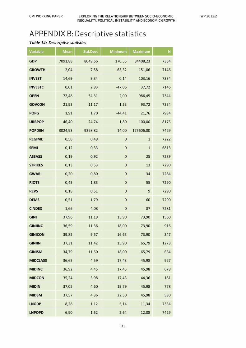
APPENDIX B: Descriptive statistics Table 14: Descriptive statistics

Variable Mean Std.Dev. Minimum Maximum N

GDP 7091,88 8049,66 170,55 84408,23 7334

GROWTH 2,04 7,58 -63,32 151,06 7146

INVEST 14,69 9,34 0,14 103,16 7334

INVESTC 0,01 2,93 -47,06 37,72 7146

OPEN 72,48 54,31 2,00 986,45 7344

GOVCON 21,93 11,17 1,53 93,72 7334

POPG 1,91 1,70 -44,41 21,76 7934

URBPOP 46,40 24,74 1,80 100,00 8175

POPDEN 3024,93 9398,82 14,00 175606,00 7429

REGIME 0,58 0,49 0 1 7222

SEMI 0,12 0,33 0 1 6813

ASSASS 0,19 0,92 0 25 7289

STRIKES 0,13 0,53 0 13 7290

GWAR 0,20 0,80 0 34 7284

RIOTS 0,45 1,83 0 55 7290

REVS 0,18 0,51 0 9 7290

DEMS 0,51 1,79 0 60 7290

CINDEX 1,66 4,08 0 87 7281

GINI 37,96 11,19 15,90 73,90 1560

GINIINC 36,59 11,36 18,00 73,90 916

GINICON 39,85 9,57 16,63 73,90 347

GINIIN 37,31 11,42 15,90 65,79 1273

GINISM 34,79 11,50 18,00 65,79 664

MIDCLASS 36,65 4,59 17,43 45,98 927

MIDINC 36,92 4,45 17,43 45,98 678

MIDCON 35,24 3,98 17,43 44,36 181

MIDIN 37,05 4,60 19,79 45,98 778

MIDSM 37,57 4,36 22,50 45,98 530

LNGDP 8,28 1,12 5,14 11,34 7334

LNPOPD 6,90 1,52 2,64 12,08 7429

CMI WORKING PAPERSThis series can be ordered from:

CMI (Chr. Michelsen Institute)Phone: +47 47 93 80 00 Fax: +47 47 93 80 01E-mail: [email protected]

P.O.Box 6033 Bedriftssenteret,N-5892 Bergen, NorwayVisiting address: Jekteviksbakken 31, Bergen

Web: www.cmi.no

Price: NOK 50Printed version: ISSN 0804-3639Electronic version: ISSN 1890-5048Printed version: ISBN 978-82-8062-428-4Electronic version: ISBN 978-82-8062-429-1

This paper is also available at:www.cmi.no/publications

The hypothesis that socio-economic inequality has a detrimental effect on economic growth by breeding political instability has been subject to empirical investigation for decades. However, the numerous studies in the field have yielded highly different conclusions, and still no agreement has been reached as to what the relationship between these variables really looks like. This study investigates why empirical studies have given such diverging results. By using several different measures both of socio-economic inequality, political instability and economic development it examines whether differences in methods and measurement can explain the variation in previous findings. It is revealed that the effect of socio-economic inequality upon political instability is dependent on which measures are used, and that the effect of instability upon economic development varies between different analytical models. The study thus shows that conclusions about the relationship between these phenomena are not robust to alternative measurement.

exploring the relationship between socio-economic ... · exploring the relationship between...

Documents