Discrete Applied Mathematics ( ) –

Contents lists available at ScienceDirect

Discrete Applied Mathematics

journal homepage: www.elsevier.com/locate/dam

Exploring the role of graph spectra in graph coloringalgorithm performanceKate Smith-Miles ∗, Davaatseren BaatarSchool of Mathematical Sciences, Monash University, Victoria 3800, Australia

a r t i c l e i n f o

Article history:Received 23 November 2012Received in revised form 5 November 2013Accepted 9 November 2013Available online xxxx

Keywords:Graph spectraGraph invariantsGraph coloringBranch and boundDSATURLP-relaxationAlgorithm selection

a b s t r a c t

This paper considers the challenge of recognizing how the properties of a graph determinethe performance of graph coloring algorithms. In particular, we examine how spectralproperties of the graphmake the graph coloring task easy or hard.We address the questionof when an exact algorithm is likely to provide a solution in a reasonable computationtime, when we are better off using a quick heuristic, and how the properties of thegraph influence algorithm performance. A new methodology is introduced to visualizea collection of graphs in an instance space defined by their properties, with an optimalfeature selection approach included to ensure that the instance space preserves thetopology of an algorithm performance metric. In this instance space we can reveal howdifferent algorithms perform across a variety of instance classes with various properties.Wedemonstrate themethodology using a sophisticated branch and bound exact algorithm,and the faster heuristic approaches of integer rounding of a linear programming relaxationof the graph coloring formulation, as well as a greedy degree-saturation heuristic. Ourresults demonstrate that spectral properties of the graph instances can provide usefuldescriptions of when each of these algorithms will provide the best solution for a givencomputational effort.

© 2013 Elsevier B.V. All rights reserved.

1. Introduction

It is a commonly held view that exact algorithms are only likely to solve small instances ofNP-hard optimization problemswithin a reasonable computation time, and that heuristics are necessary for larger instances [68]. Likewise, it is frequentlyassumed that heuristics are unlikely to give exact solutions, but will quickly converge to near-optimal solutions. Both ofthese assumptions should be challenged, since instance size is not the only determinant of whether an exact algorithmwill find an instance easy or hard to solve, nor whether a heuristic will find a near-optimal solution. Much research hasbeen conducted on what makes optimization problems hard [38] and the role of certain properties of the instances thatcontribute to phase transition boundaries [14,23,1,28], whereby an instance becomes harder to solve as a key property ofthe instance is changed, such as edge density in graph coloring [1]. A recent survey has described a comprehensive collectionof features that determine hardness for a wide range of common optimization problems [54], and showed that instancesize is frequently not the only significant feature, with other properties like correlation coefficients playing an importantrole [3,30].

The No-Free-Lunch (NFL) Theorems [64,17] tell us that any general algorithm will find some instance classes difficultcompared to another algorithm that exploits some prior knowledge of the characteristics of an instance class. From this ideahas come an approach known as algorithm portfolios [37,36], whereby training data is used to build a model that predicts

∗ Corresponding author. Tel.: +61 3 99053170; fax: +61 3 99054403.E-mail addresses: kate.smith-miles@monash.edu, kate.smithmiles@gmail.com (K. Smith-Miles).

0166-218X/$ – see front matter© 2013 Elsevier B.V. All rights reserved.http://dx.doi.org/10.1016/j.dam.2013.11.005

2 K. Smith-Miles, D. Baatar / Discrete Applied Mathematics ( ) –

how each of a collection of algorithms is likely to perform for a given instance, based on measurable properties, and themodel is then used on unseen data to predict the best algorithm. This approach has proven to be a powerful one, winningvarious competitions [66,67,43,41], and helps to circumvent the NFL Theorem by ensuring that knowledge of the instanceproperties is considered by a meta-algorithm.

These ideas date back to the 1970s, when the Algorithm Selection Problem (ASP) was first posed by Rice [49], andformulated as the task of learning the relationship between a set of features describing problem classes, and the performanceof algorithms. The approach was then applied to the task of selecting the best solver for partial differential equations andnumerical quadrature [61,32,33,47]. Independently, the same ideas have been applied in the machine learning community,to select the best algorithm for solving classification [10,2] and prediction problems [46,63]—a sub-field known as meta-learning [62] since the approach is to learn about learning algorithm performance. A discussion about how these ideas havebeen applied to a variety of fields of research can be found in Smith-Miles [51].

More recently, we have been applying these ideas to understand how optimization algorithm performance is affectedby instance properties, considering the Travelling Salesman Problem [56], Scheduling [52], timetabling [53], quadraticassignment problems [50], and graph coloring [57]. The latter paper considered two heuristics: a degree saturation graphcoloring heuristic called DSATUR [65] and a tabu search heuristic downloaded from Culberson’s web resources for graphcoloring [18]. The analysis showed that the best algorithm for the five sets of instance classes from Culberson’s instancegenerators [18] could be predicted quite accurately (more than 93% accuracy on out-of-sample testing) using some simpleproperties of graphs. The region in instance space where each algorithm outperforms the other is known as the algorithmfootprint [16], and we have previously provided a methodology for quantifying the area of each algorithm’s footprint as acomparative measure of performance [55].

In this paper, we extend this work to consider how such an approach can be used to determine when an exact algorithmcan be expected to deliver a solution within a reasonable computation time, and when a quick heuristic might be expectedto be more productive. If a heuristic can obtain the same solution as an exact approach in a much quicker time, then theexact algorithm is unnecessary and not worth the wait. We ask the question, under what conditions of a graph instance canwe expect that a sophisticated exact algorithm will be worth the computational effort? Our exact algorithm is a branch-and-bound approach [39] which utilizes the DSATUR heuristic and involves solving the linear programming (LP) relaxation atthe root node. So we can consider that this sophisticated exact algorithm has some exit points where we could terminatewith a heuristic solution. In this paper we also extend the collection of properties of the graph to consider many spectralfeatures, as well as other invariant graph properties that have been proposed recently to enable new conjectures to beformed about graphs [12]. We augment our previous methodology to include, not just machine learning of the relationshipsbetween features and algorithm performance, but a visual exploration of a well-defined instance space. This instance spaceis created by performing optimal feature selection in amanner that projects the instances to a two-dimensional spacewherethe algorithm performance has been topologically preserved. Inspection of the distribution of features across this instancespace permits insights to be formed about how certain features are influencing algorithm performance in a way that ishidden from standard machine learning approaches to predicting the winning algorithm.

In Section 2we briefly describe the task of graph coloring and discuss the branch-and-bound algorithm and heuristics weconsider in this paper. In Section 3 we then present the framework of the Algorithm Selection Problem [49,51] that enablesour graph coloring algorithm investigation to be described, including the instances, features, algorithms, and performancemetrics. Section 4 proposes the methodology for generating a topology preserving instance space via optimal featureselection to enable clear visualization of the algorithm footprints and the impact of the chosen features. Experimental resultsare presented in Section 5 to demonstrate the methodology, and Conclusions and future research directions are discussedin Section 6.

2. Graph coloring algorithms

A graph G = (V , E) comprises a set of vertices V and a set of edges E that connect certain pairs of vertices. The graphcoloring problem (GCP) is to assign colors to the vertices, minimizing the number of colors used, subject to the constraintthat two vertices connected by an edge (called adjacent vertices) do not share the same color. The optimal (minimal) numberof colors needed to solve this NP-complete problem is called the chromatic number of the graph. Graph coloring findsimportant applications in problems such as timetabling, where events to be scheduled are represented as vertices, withedges representing conflicts between events, and the color representing the time period [13,19].

Due to the NP-completeness of this problem, many heuristics have been designed [45,22]. One of the earliest heuristicswas DSATUR [11,65], which was shown to be exact for bipartite graphs. The saturation degree of a vertex is defined to be thenumber of different colors to which it is adjacent. The DSATUR (degree saturation) heuristic is a simple approach to coloringa graph is shown in Algorithm 1.

For non-bipartite graphs though, the performance of DSATUR is not optimal, and many more sophisticated searchstrategies have been employed to provide effective heuristics for general graphs, including tabu search [29], simulatedannealing [34], iterated local search [15], scatter search [26], genetic algorithms [21], and hybrid approaches [20,9]. Just asthe performance of DSATUR depends on the bipartivity of the graph, we should also expect the performance of any methodto depend on various properties of the graph, but the relationship between the properties of the graph and the performance

K. Smith-Miles, D. Baatar / Discrete Applied Mathematics ( ) – 3

Algorithm 1 DSATURStep 1: Arrange the vertices by decreasing order of degrees.Step 2: Color a vertex of maximal degree with color 1.Step 3: Choose an uncolored vertex with a maximal saturation degree, while breaking ties arbitrarily.Step 4: Color the chosen vertex with the least possible (lowest numbered) color.Step 5: If all the vertices are colored, stop. Otherwise, return to Step 3.

of various heuristics is not well understood. Empirical analysis of algorithms is needed [31], particularly to understand thecomplex relationship between graph properties, instance generators, and algorithm performance.

In this paper we reimplement and use the well known exact algorithm for graph coloring problem by Mehrotra andTrick [39]. This is one of the best exact algorithms for the graph coloring problem, formulated using independent sets as

mins∈S

xs

s.t.s:v∈s

xs ≥ 1 ∀v ∈ V (1)

xs ∈ {0, 1} ∀s ∈ S

where S is the set of all maximal independent sets.The constraints (1) ensure that each vertex is covered by at least one independent set. A column generation and a branch

and bound approach (B&B) were used to solve the (0–1) linear programming problem. This approach used Zykov contractionand insertion branching scheme [69,24]. Here we briefly describe the approach and more details can be found in [39].

At each node of the B&B tree the LP-relaxation of the current problem is solved using a column generation approach.New columns with negative reduced costs are generated by solving a maximum weighted independent set problem. Sincethis is itself an NP-hard problem, the new columns are generated using a greedy type of heuristic and an exact enumerativealgorithm is applied only if the heuristic fails to generate a column with negative reduced cost. The exact algorithm forthe maximum weighted independent set problem terminates as soon as a column with negative reduced costs is found.Moreover, the LP-relaxation is solved exactly only at the root node, and for the remaining nodes the column generation isterminated as soon as the objective value falls below the upper bound obtained at the root node. We call this heuristic atthe root node LPround.

At any node, we can use the solution of the LP relaxation to obtain a feasible coloring, providing an upper bound to theGCP by using a simple heuristic to round the non-integer components of the LP solution to the nearest integer solution.

Due to the Zykov branching scheme, at each node we solve a GCP similar to its parent node GCP. In [27], Hansen et al.noted that simple preprocessing at each node of the branch and bound tree can speed up the computation. Thus, at eachnode of the tree, we use preprocessing to remove universal, dominated, and isolated vertices from the current graph toproduce a pre-processed graph G′(V ′, E ′). Moreover, at each node we use the greedy DSATUR algorithm [11], to obtain aninitial upper bound. The lower bound at each node is obtained by calculating the maximum clique size of the graph, usingthe algorithm proposed in [44].

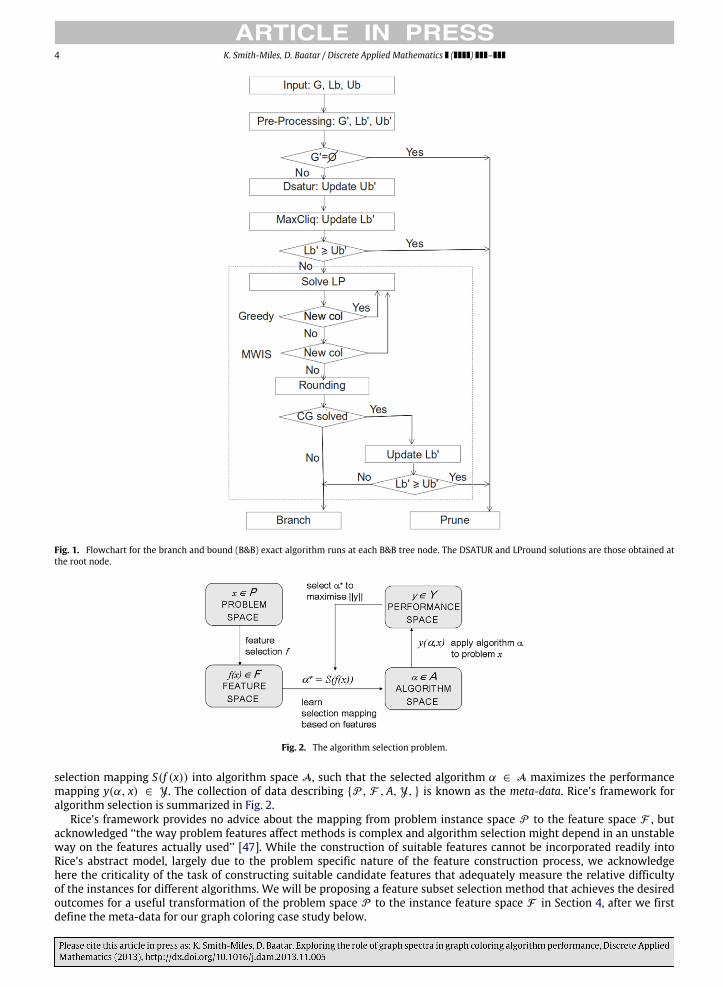
The entire process at each node of the B&B tree is described in Fig. 1, showing that DSATUR and LP-relaxation are used ateachnode to update theupper and lower bounds.We take theDSATURand LPround solutions at the root node as theheuristicsolutions bywhichwe compare the effectiveness of the B&B algorithm. Our implementation produced for this paper obtainsvery similar results to those reported in [39], and the executable code is available upon request. In the following section, wepresent the framework we will use to determine how the properties of the graph instances, including spectral properties,determine the effectiveness of this exact algorithm compared to the simple heuristics DSATUR and LPround. While we areconsidering the GCP with B&B and heuristics for this paper, the methodology is broadly applicable to a wider range ofalgorithms and problem domains.

3. Algorithm selection framework

In 1976, Rice [49] proposed a framework for the Algorithm Selection Problem (ASP), which seeks to predict whichalgorithm from a portfolio is likely to perform best based onmeasurable features of a collection of problem instances. Thereare four essential components of the model:

• the problem space P represents the set of instances of a problem;• the feature spaceF containsmeasurable characteristics of the instances generated by a computational feature extraction

process applied to P ;• the algorithm space A is the set (portfolio) of all algorithms for tackling the problem considered by the study;• the performance space Y represents the mapping of each algorithm to a set of performance metrics.

In addition, we need to find a mechanism for generating the mapping from feature space to algorithm space. The AlgorithmSelection Problem can be formally stated as: for a given problem instance x ∈ P , with feature vector f (x) ∈ F , find the

4 K. Smith-Miles, D. Baatar / Discrete Applied Mathematics ( ) –

Fig. 1. Flowchart for the branch and bound (B&B) exact algorithm runs at each B&B tree node. The DSATUR and LPround solutions are those obtained atthe root node.

Fig. 2. The algorithm selection problem.

selection mapping S(f (x)) into algorithm space A, such that the selected algorithm α ∈ A maximizes the performancemapping y(α, x) ∈ Y. The collection of data describing {P , F , A, Y, } is known as the meta-data. Rice’s framework foralgorithm selection is summarized in Fig. 2.

Rice’s framework provides no advice about the mapping from problem instance space P to the feature space F , butacknowledged ‘‘the way problem features affect methods is complex and algorithm selection might depend in an unstableway on the features actually used’’ [47]. While the construction of suitable features cannot be incorporated readily intoRice’s abstract model, largely due to the problem specific nature of the feature construction process, we acknowledgehere the criticality of the task of constructing suitable candidate features that adequately measure the relative difficultyof the instances for different algorithms. We will be proposing a feature subset selection method that achieves the desiredoutcomes for a useful transformation of the problem space P to the instance feature space F in Section 4, after we firstdefine the meta-data for our graph coloring case study below.

K. Smith-Miles, D. Baatar / Discrete Applied Mathematics ( ) – 5

3.1. Graph coloring problem instances (P )

The problem instances we have used in this research consist of 800 instances comprising:

• 125 benchmark instances widely used by many researchers. 89 of the instances are considered to be hard problems.Benchmark instances consist of different types of graphs such as Leighton, flat, Mycielski, queen, miles, game, register,insertions etc. A full description of the instances can be obtained from http://mat.gsia.cmu.edu/COLOR03/.

• 375 random graph instances, generated using the open source generator Networkx. A random graph G(n, p) chooseseach of the possible edges with probability p. For a given number of vertices n, we generate 5 random graphs for each ofp ∈ {0.1, 0.3, 0.5, 0.7, 0.9}, resulting in 125 instances for each of n ∈ {30, 50, 70}.

• 300 geometric graph instances, generated using Networkx. A geometric graph G(n, r) places n vertices uniformly atrandom in a unit cube, and connects two vertices u and v with an edge if d(u, v) ≤ r , where d is the Euclidean distanceand r is a radius threshold. We generate 25 repetitions of G(n, r) graphs with r ∈ {0.1, 0.4, 0.6, 0.9}, resulting in 100geometric graph instances for each of n ∈ {100, 150, 200}. Further information about the Networkx generators can befound athttp://networkx.lanl.gov/reference/generators.html.

Empirical studies have already shown how the performance of some algorithms depends on the source of the instances.Observations include the fact that DSATUR seems to outperform othermethods such as tabu search and simulated annealingon geometric graphs [34]. This was conjectured to be due to the easiness of coloring graphs with large cliques [6], with thegirth and degree inhibited and weight-biased graphs designed to prove more difficult for DSATUR, as shown in our previouswork [57] which used a different set of Culberson’s instances [18]. Culberson states about his resources for graph coloring,‘‘My intention is to provide several graph generators that will support empirical research into the characteristics of variouscoloring algorithms. Thus, I want generators that will exhibit variations of various characteristics of graphs, such as degree(expectation and variation), hidden colorings, girth, edge distributions etc.’’. Indeed, when the instances are intentionallygenerated to exhibit a diversity of properties, it is relatively straightforward to identify the classes of instances where onealgorithm outperforms others, as we have already demonstrated [57]. In this research, we are using instances that are farless controlled for diversity, and algorithms that are less diverse in their behaviors (given that the B&B algorithm uses theresults of DSATUR and LP-relaxation to construct its solution). Unlike in our previous work, where we have used geneticalgorithms to evolve instances for optimization problems that are intentionally easy or hard [56], we aim here to developa methodology that enables a rich set of instance features to distinguish between algorithm performance using commoninstances.

3.2. Graph properties or features (F )

A recent survey of what makes optimization problem instances difficult [54] shows that there are many features orproperties of a graph that can be calculated in polynomial time, that could be used to shed some light on the relationshipsbetween graph instances and algorithmperformance.Many of these features are based on properties of the adjacencymatrixA and Laplacianmatrix L of the graphG(V , E) defined as follows: Ai,j = 1 if an edge connects vertices i and j, and 0 otherwise;Li,i = degree(Vi), Li,j=i = −1 if an edge connects vertices i and j, and 0 otherwise.

Graph theory researchers have long collected interesting graphs [48] which are used to develop new conjectures, andoften provide counter-examples to existing theorems. Recently, several exciting developments have occurred where graphswith specific properties can be generated from an extendable database—known as House of Graphs [12]. These graphs havebeen used successfully to generate new conjectures by generating linear inequalities that describe the relationships betweenspecific graph properties known as invariants [40]. In this studywe consider many of the invariant graph properties referredto by House of Graphs, as well as some additional spectral features based on the eigenvalues of the adjacency and Laplacianmatrices of the graph. While this is not an exhaustive list of all features relevant to graph coloring difficulty, we believe ourchosen graph properties are comprehensive enough to demonstrate the proposed methodology.

For the graph G = (V , E), we consider the following 21 features:

1. The number of vertices in a graph: n = |V |.2. The number of edges in a graph: |E|.3. The diameter of a graph: the greatest distance between any pair of vertices. To find the diameter we find the shortest

path between each pair of vertices and take the greatest length of these paths.4. The density of a graph: the ratio of the number of edges to the number of possible edges ρ =

2|E|

n(n−1) .5. Average path length: the average number of steps along the shortest paths for all possible pairs of vertices. It is ameasure

of the efficiency of traveling between vertices.6. Mean vertex degree: the number of connections a vertex has to other vertices.7. Standard deviation of vertex degree: the average vertex degree and its standard deviation can give us an idea of how

connected a graph is.8. The clustering coefficient: a measure of degree to which vertices in a graph tend to cluster together. This is a ratio of the

closed triplets to the total number of triplets in a graph. A closed triplet is a triangle, while an open triplet is a trianglewithout one side [58].

6 K. Smith-Miles, D. Baatar / Discrete Applied Mathematics ( ) –

9. Energy: the mean of the absolute values of the eigenvalues of the adjacency matrix [4].10. Standard deviation of the set of eigenvalues of the adjacency matrix:11. Algebraic connectivity: the second smallest eigenvalue of the Laplacian matrix [42]. This reflects how well connected a

graph is. Cheeger’s constant, another important graph property, is bounded by half the algebraic connectivity [8].12. Smallest non-zero eigenvalue of the Laplacian matrix.13. Second smallest non-zero eigenvalue of the Laplacian matrix.14. Largest eigenvalue of the Laplacian matrix.15. Second largest eigenvalue of the Laplacian matrix.16. Smallest eigenvalue of the adjacency matrix.17. Second smallest eigenvalue of the adjacency matrix.18. Largest eigenvalue of the adjacency matrix.19. Second largest eigenvalue of the adjacency matrix.20. Gap between the largest and second largest eigenvalues of the adjacency matrix.21. Gap between the largest and smallest non-zero eigenvalues of the Laplacian matrix.

3.3. Algorithms (A)

As described in Section 2 and Fig. 1, we have implemented the branch and bound exact algorithm of Mehrotra andTrick [39], which also involves calculating heuristic solutions for each instance for the DSATUR heuristic [11] implementedaccording to Algorithm 1, and a simple LPround heuristic based on rounding the LP-relaxation solution. Thus, the set ofalgorithms in the portfolio for this paper is {B&B, DSATUR, LPround}.

3.4. Performance metric (Y)

The performance of an algorithm can be defined in many different ways depending on the goals. We might say thatone algorithm is better than another if it finds the same quality solution in a faster time, or if it obtains a much betterquality solution for the same run-time. How we define ‘‘same quality’’ may involve some tolerance, and we can define thismore specifically if we introduce concepts like ‘‘two algorithms give the same result if their solutions are within ϵ% of eachother’’. Acknowledging the arbitrariness of this decision, and without loss of generality, in this paper wemeasure algorithmperformance using a combined measure of the cpu time and the relative gap (gap in the number of colors found by analgorithm and the best known lower bound), as follows. Let Yi be the measured performance of algorithm i in the portfoliogiven a maximum time limit of 1800 s, which takes β seconds to converge to a solution that has a gap of α% from the bestlower bound obtained from the remaining nodes of the final branch and bound tree. Thenwe define the performancemetricas:

Yi = β + 1800α. (2)

In our research we have restricted the computation time for the algorithm, i.e. the algorithm is aborted when it reachesthe time limit of 1800 s or the best known solution is obtained. Therefore, the above definition of performance can be seenas a lexicographical measure with respect to gap α and computation time β . If the problem is solved exactly (α = 0) withinthe time limit then a shorter computation time β indicates an easier instance, and if the algorithm reaches the time limitthen the relative gap α is used to weight the algorithm performance.

3.5. Experimental meta-data

We are now in a position to fully describe the meta-data for our experimental analysis using the framework proposed inRice [49], and adapted for the study of optimization algorithm performance by Smith-Miles [51].

• The problem spaceP is a set of 800 graph coloring instances, from benchmark instances and random and geometric graphgenerators, with the number of vertices in the range [11, 2419], as described in Section 3.1.

• The algorithm space A comprises one exact algorithm (B&B) and two heuristics: DSATUR and LPround described inSection 2.

• The performance space Y is a lexicographic metric given by Eq. (2) that considers the minimum number of colors foundby an algorithm after a maximum of 1800 s of run-time, expressed as a gap to the best lower bound from the remainingnodes of the final branch and bound tree.

• The feature space F is defined by the 21 invariant graph properties listed in Section 3.2.

The starting point for empirical analysis based on this meta-data is typically to use machine learning methods to learn topredict the performance metric Yi in terms of the features F for each algorithm i. Using linear regression for this approach,we obtain a coefficient of determination R2

= 0.67 for predicting the performance metric given by Eq. (2) for the B&Balgorithm with the 21 features as independent variables. This is not a strong predictive performance. If we consider theperformance metrics for each algorithm to determine the best algorithm (by choosing for each instance the algorithm that

K. Smith-Miles, D. Baatar / Discrete Applied Mathematics ( ) – 7

gives the minimal α, followed by the smallest β to break ties), and then use a standard classification algorithm such as aNaive Bayes classifier to predict which algorithm will be best for a given instance based on the 21 features, we find that theclassification accuracy is only around 60%, again a poor predictive performance. If the predictive performance was higher,we would be satisfied that the features explain algorithm performance, and we could consider rule-based learners to try toextract rules describing how features affect performance, as we have done in our previous work [57]. In this case, however,the standard machine learning approach has not yielded much insight, and we need to develop a new methodology thatenables us to see how graph properties are influencing algorithm performance.

4. Methodology

Our goal is to identify the various types of instances within the high-dimensional feature space and to understand thedependence of algorithm performance on the properties of the instances. In order to visualize the high dimensional featurespace (defined by the set of 21 candidate features discussed in Section 3.2), we need to develop a method to project theinstances into a two-dimensional plane thatmaintains the relationships between the instances in feature space, and enablesus to create a projectionwhere the algorithmperformancemetric is smoothly varying across the plane sowe can easily locatethe easy and hard instances and explore how the features are distributed across the same space.

Reducing the feature set from 21 features to 2 features for ease of visualization can be achieved by either selecting thetwo most significant features, or by creating two new features that combine some of the 21 features in a manner that bestachieves our goal of topology preservation. We adopt the latter approach and propose a methodology that involves optimalfeature subset selection combined with principal component analysis to visualize the instances in a two-dimensional planedefined by two new independent features that are linear combinations of the optimally selected subset of features. Wecan then examine the location of the instance classes, and study how the smoothly varying algorithm performance metriccorrelates with the distribution of the features across the instance space. The footprint of each algorithm can also beidentified in this manner. We now describe details of each step of the methodology.

4.1. Optimal feature subset selection

Successful solution of the ASP depends critically on being able to learn the mapping S between feature space F andperformance space Y. The ASP can be recast as a classification problem, if we are focused on predicting the best algorithm,or as a regression problem if we are more concerned with algorithm ranking. In order to learn the mapping S, we need toensure that the set of feature vectors in the meta-data is indeed discriminatory and can be used to achieve a satisfactoryclassification or prediction, and we focus now on the requirements for selecting the optimal subset of features F ∗

⊆ F .We present this merely to extend the framework of Rice to consider the question of feature selection, using the notationestablished in Section 3, rather than to provide a comprehensive review of feature selection methods which is available inother papers (see [25] for example).

Generally, feature selection is a two-step process: first we need to define how we will measure the goodness of aparticular subset of features, and once this metric is determined, we can utilize an optimization search strategy to find thesubset F ∗ that maximizes the goodness metric. In this paper, we define the goodness of a subset of features based on theextent towhich instanceswith similar performance are close together in the instance space defined by the subset of features.In other words, we require that the choice of features F ∗ enables us to see the algorithm performance change smoothly aswe move across the instance space. However, mathematically it is difficult to present this requirement efficiently. Here weuse the following definition of lack of smoothness of performance for a subset of the features F ∗:

x∈P

|Y(x) − Y(Nx(F∗, k))| (3)

where Nx defines the set of k nearest neighbors of the instance x in the instance space obtained using the subset F ∗, andY(Nx) defines the mean algorithm performance in the neighborhood of x.

If an instance is surrounded by other instances with similar algorithm performances then the mean of the performancesof the neighbors tends to be close to the algorithm performance of the instance, and the smoothness if maximized (Eq. (3)is minimized). Thus, the most effective feature subsets F ∗ will have the smallest metric defined by Eq. (3).

For any fixed number of selected features m, we use a genetic algorithm to find the best subset with m features, usinga fitness function related to minimizing Eq. (3). Among the best subsets obtained for each m = 2, . . . , 21 we select the setwith the smallest sum according to Eq. (3).

Other researchers have used similar intuitive ideas for feature subset selection formachine learning tasks [60,7], but haveutilized information theory metrics, particularly for the discrete classification task of identifying which features enable theclass label define best performing algorithm to be predicted most accurately. Our smoothness metric is well suited to ourtask of examining a continuous assessment of algorithm performance, but the metric could easily be modified without lossof generality of the methodology.

8 K. Smith-Miles, D. Baatar / Discrete Applied Mathematics ( ) –

4.2. Projection of instances

Once we have selected the best m features as the subset F ∗, we can either use machine learning methods to achievealgorithm selection and performance prediction in Rm, which is still difficult to visualize, or we can utilize dimensionreduction techniques to project the instances to R2, ensuring that we are not losing too much information. Here, we useprincipal component analysis (PCA) [35], which essentially rotates the data to a new coordinate system in Rm, with axesdefined by m new features which are linear combinations of the m selected features in F ∗, calculated as the eigenvectorsof them × m covariance matrix; we then project the instances on the two principal eigenvectors corresponding to the twolargest eigenvalues of the covariance matrix. Reducing the description of each instance from a vector in Rm to a vector inR2 has most certainly cost us a loss of information, and we measure the loss in terms of how much of the variance found inthe data cannot be explained by the first two eigenvectors. The first two eigenvalues explain a percentage of the variationin the data given by (λ1+λ2)m

i=1 λi. We will consider that the new two-dimensional instance space is an adequate representation

of the original feature space if most of the variation in the data is explained by these two principal axes.

4.3. Exploring the instance space

The instance space is now populated by a set of 800 graph coloring instances, each defined by a set of 21 features relatedto the graph properties, but projected to a two-dimensional plane after selecting the best subset of features upon which toperform principal component analysis. Instances that are similar in properties, as well as similar in algorithm performance,are located near each other, and we are now in a position to explore the instance space to understand how the location ofdifferent types of instances in this space reveals the relationships between features and algorithm performance. Specifically,we will be gaining such insights by:

1. examining the location of the different types of instances in the instance space;2. examining the distribution of the performancemetric across the instance space, for each algorithm, to understandwhere

the easy and hard instances are located;3. examining the distribution of each feature across the space and looking for visual correlations to algorithm performance;4. identifying the best performing algorithm for regions of the instance space (either through machine learning methods

or visual inspection);5. drawing conclusions aboutwhich features affect algorithmperformance, andwheneach algorithm is expected to perform

best.

In the following section we demonstrate this methodology using the meta-data summarized in Section 3.5.

5. Experimental results

5.1. Parameter settings

From the raw meta-data we first applied a log transform to all features to reign in the effect of outliers in the instancespace, and then normalized all features to [0, 1] using min–max normalization. When running the B&B algorithm, we setthe time limit to be 1800 s in total, but to speed up computation we imposed a time limit of 180 s for the enumerativealgorithm for the maximum clique (MC) sub-problem. However, the algorithm provided exact solutions for all instancesexcept one. In order to generate new columns with negative reduced cost we used a greedy approach with 3 differentstrategies. The exact enumerative algorithm for themaximumweighted independent set (MWIS) problemwas applied onlyif the heuristics failed to produce a new column.We set the time limit to 300 s for theMWIS problem for all nodes except theroot node. As mentioned earlier, the LP-relaxation was solved exactly only at the root node and for the remaining nodes thecolumn generation was terminated early if there was no significant improvement of the objective value in last 50 columngenerations or the time limitwas reached for theMWIS problem. In the latter case,when columngenerationwas terminated,we proceeded to branch the node. This strategy provided the opportunity to explore more nodes, rather than spending toomuch time at any one node, and improved the computation time. At each node we used greedy heuristics to construct aninteger solution from the solution of the LP.

For the feature subset selection, the genetic algorithm was implemented using the MATLAB optimization toolbox. Eachselection of subsets (individuals) was represented using a binary vector to indicate if a candidate feature was a memberof the subset. If the number of distinct possible subsets with m features was greater than 50, then the genetic algorithmwas run with population size 50 for 100 generations. Otherwise, the initial population consisted of all possible distinctindividuals and the best individual was selected based on the smoothness measure, i.e. the initial generation consisted ofall distinct individuals. To define the neighborhood of an instance we used k nearest neighbors with k = 10, with the metricbeing Euclidean distance in the 2-dimensional instance space defined by the two largest principal components. As a fitnessfunctionweminimized the average non-smoothness across the 2-dimensional instance space, i.e. the total non-smoothnessgiven by Eq. (3) divided by the total number of instances. Thus, the feature selection process involved performing PCA foreach individual subset being evaluated by the genetic algorithm, in an iterative process.

K. Smith-Miles, D. Baatar / Discrete Applied Mathematics ( ) – 9

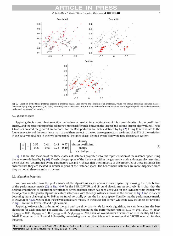
Fig. 3. Location of the three instance classes in instance space. Gray shows the location of all instances, while red shows particular instance classes:benchmark (top left), geometric (top right), random (bottom left). (For interpretation of the references to colour in this figure legend, the reader is referredto the web version of this article.)

5.2. Instance space

Applying the feature subset selection methodology resulted in an optimal set of 4 features: density, cluster coefficient,energy, and the spectral gap of the adjacency matrix (difference between the largest and second largest eigenvalues). These4 features created the greatest smoothness for the B&B performance metric defined by Eq. (2). Using PCA to rotate to thefour eigenvectors of the covariance matrix, and then project to the top two eigenvectors, we found that 91% of the variationin the data was retained in the two-dimensional instance space, defined by the following new coordinate system:

v1v2

=

0.55 0.44 0.42 0.57

−0.23 −0.63 0.72 0.19

densitycluster coefficient

energyspectral gap

. (4)

Fig. 3 shows the location of the three classes of instances projected into this representation of the instance space usingthe new axes defined by Eq. (4). Clearly, the grouping of the instances within the geometric and random graph classes intodense clusters (determined by the parameters n, p and r) shows that the similarity of the properties of these instances hasensured that they are located in similar regions of the instance space. The benchmark instances are more dispersed sincethey do not all share a similar structure.

5.3. Algorithm footprints

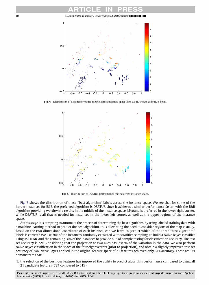
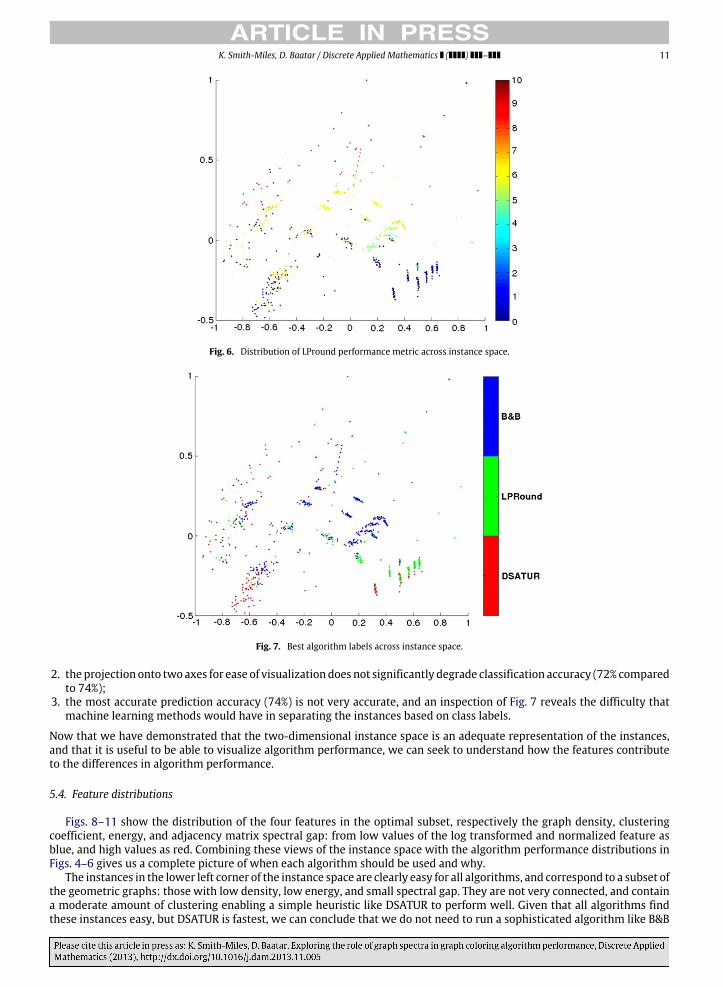
We now consider how the performance of the algorithms varies across instance space, by showing the distributionof the performance metric (2) in Figs. 4–6 for the B&B, DSATUR and LPround algorithms respectively. It is clear that thedesired smoothness of algorithm performance across instance space has been achieved for the B&B algorithm (which wasthe objective of the genetic algorithm feature selection), with the easy instances shown at the bottom of Fig. 4 and instancesbecoming more challenging for B&B as we travel vertically across the instance space. Considering the performance metricof DSATUR in Fig. 5, we see that the easy instances are mostly in the lower left corner, while the easy instances for LProundin Fig. 6 are in the lower left and right corners.

Applying lexicographic ordering of the gap and cpu time pair (α, β) for each algorithm, we can determine the bestalgorithm for each instance. For example, if an instance generated the performance results: αB&B = 0.01, βB&B = 1600,αDSATUR = 0.01, βDSATUR = 100, αLPround = 0.05, βLPround = 200, then we would order first based on α to identify B&B andDSATUR as better than LPround, followed by an ordering based on β which would determine that DSATUR was best for thatinstance.

10 K. Smith-Miles, D. Baatar / Discrete Applied Mathematics ( ) –

Fig. 4. Distribution of B&B performance metric across instance space (low value, shown as blue, is best).

Fig. 5. Distribution of DSATUR performance metric across instance space.

Fig. 7 shows the distribution of these ‘‘best algorithm’’ labels across the instance space. We see that for some of theharder instances for B&B, the preferred algorithm is DSATUR since it achieves a similar performance faster, with the B&Balgorithm providing worthwhile results in the middle of the instance space. LPround is preferred in the lower right corner,while DSATUR is all that is needed for instances in the lower left corner, as well as the upper regions of the instancespace.

At this stage it is tempting to automate the process of determining the best algorithm, by using labeled training data witha machine learning method to predict the best algorithm, thus alleviating the need to consider regions of the map visually.Based on the two-dimensional coordinate of each instance, can we learn to predict which of the three ‘‘best algorithm’’labels is correct? We use 70% of the instances, randomly extracted with stratified sampling, to build a Naive Bayes classifierusing MATLAB, and the remaining 30% of the instances to provide out-of-sample testing for classification accuracy. The testset accuracy is 72%. Considering that the projection to two axes has lost 9% of the variation in the data, we also performNaive Bayes classification in the space of the four eigenvectors (prior to projection), and obtain a slightly improved test setaccuracy of 74%. Naive Bayes applied in the original feature space of 21 features achieved only 61% accuracy. These resultsdemonstrate that:

1. the selection of the best four features has improved the ability to predict algorithm performance compared to using all21 candidate features (72% compared to 61%);

K. Smith-Miles, D. Baatar / Discrete Applied Mathematics ( ) – 11

Fig. 6. Distribution of LPround performance metric across instance space.

Fig. 7. Best algorithm labels across instance space.

2. the projection onto twoaxes for ease of visualizationdoes not significantly degrade classification accuracy (72% comparedto 74%);

3. the most accurate prediction accuracy (74%) is not very accurate, and an inspection of Fig. 7 reveals the difficulty thatmachine learning methods would have in separating the instances based on class labels.

Now that we have demonstrated that the two-dimensional instance space is an adequate representation of the instances,and that it is useful to be able to visualize algorithm performance, we can seek to understand how the features contributeto the differences in algorithm performance.

5.4. Feature distributions

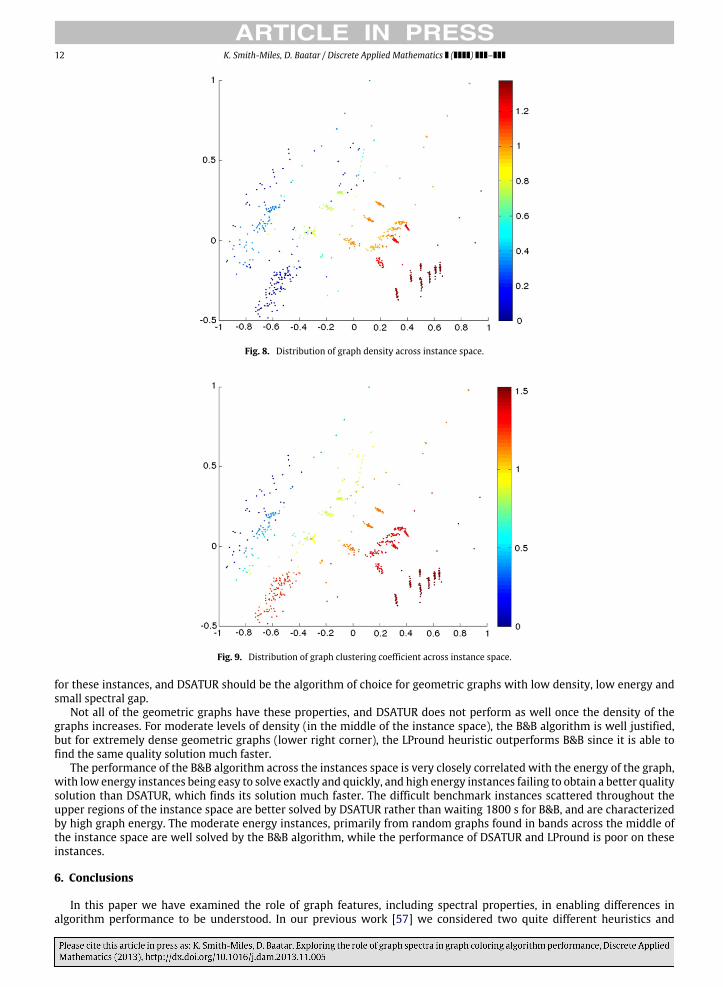
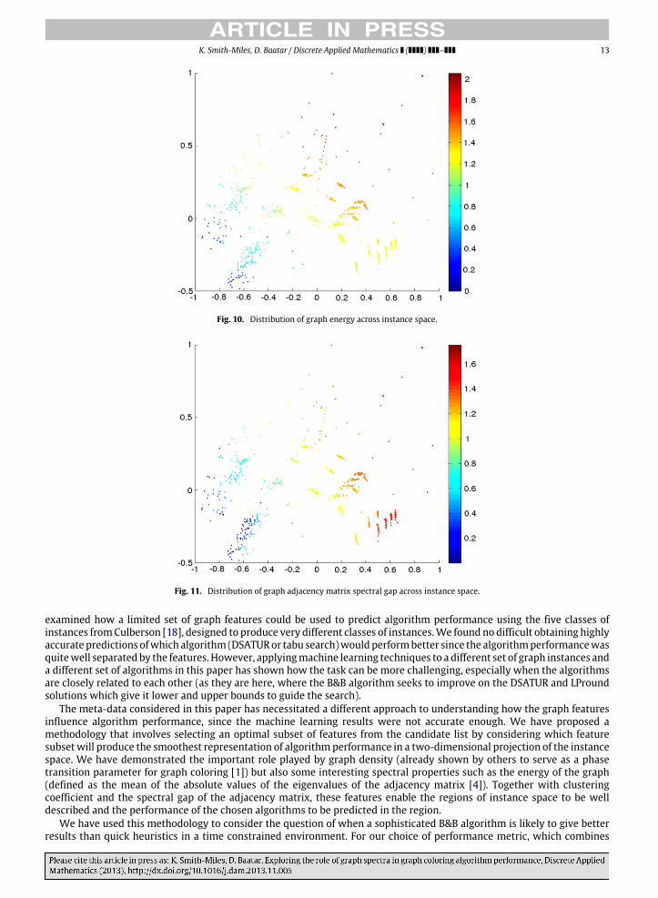
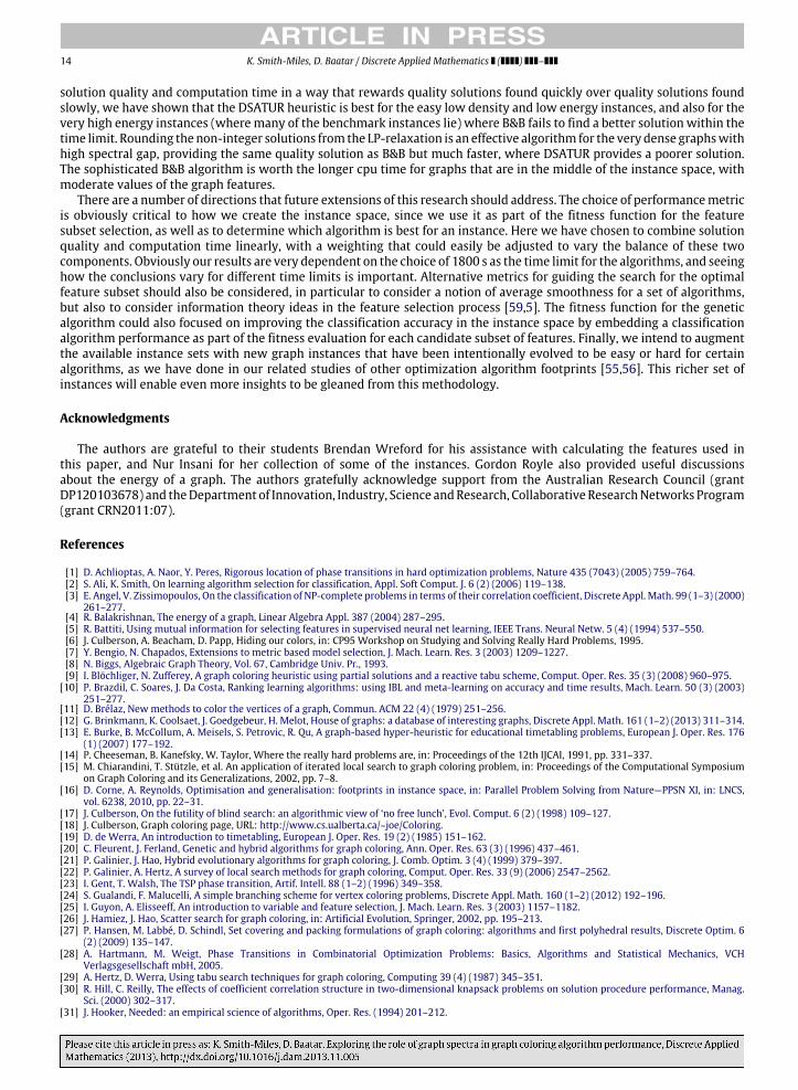
Figs. 8–11 show the distribution of the four features in the optimal subset, respectively the graph density, clusteringcoefficient, energy, and adjacency matrix spectral gap: from low values of the log transformed and normalized feature asblue, and high values as red. Combining these views of the instance space with the algorithm performance distributions inFigs. 4–6 gives us a complete picture of when each algorithm should be used and why.

The instances in the lower left corner of the instance space are clearly easy for all algorithms, and correspond to a subset ofthe geometric graphs: those with low density, low energy, and small spectral gap. They are not very connected, and containa moderate amount of clustering enabling a simple heuristic like DSATUR to perform well. Given that all algorithms findthese instances easy, but DSATUR is fastest, we can conclude that we do not need to run a sophisticated algorithm like B&B

12 K. Smith-Miles, D. Baatar / Discrete Applied Mathematics ( ) –

Fig. 8. Distribution of graph density across instance space.

Fig. 9. Distribution of graph clustering coefficient across instance space.

for these instances, and DSATUR should be the algorithm of choice for geometric graphs with low density, low energy andsmall spectral gap.

Not all of the geometric graphs have these properties, and DSATUR does not perform as well once the density of thegraphs increases. For moderate levels of density (in the middle of the instance space), the B&B algorithm is well justified,but for extremely dense geometric graphs (lower right corner), the LPround heuristic outperforms B&B since it is able tofind the same quality solution much faster.

The performance of the B&B algorithm across the instances space is very closely correlated with the energy of the graph,with low energy instances being easy to solve exactly and quickly, and high energy instances failing to obtain a better qualitysolution than DSATUR, which finds its solution much faster. The difficult benchmark instances scattered throughout theupper regions of the instance space are better solved by DSATUR rather than waiting 1800 s for B&B, and are characterizedby high graph energy. The moderate energy instances, primarily from random graphs found in bands across the middle ofthe instance space are well solved by the B&B algorithm, while the performance of DSATUR and LPround is poor on theseinstances.

6. Conclusions

In this paper we have examined the role of graph features, including spectral properties, in enabling differences inalgorithm performance to be understood. In our previous work [57] we considered two quite different heuristics and

K. Smith-Miles, D. Baatar / Discrete Applied Mathematics ( ) – 13

Fig. 10. Distribution of graph energy across instance space.

Fig. 11. Distribution of graph adjacency matrix spectral gap across instance space.

examined how a limited set of graph features could be used to predict algorithm performance using the five classes ofinstances fromCulberson [18], designed to produce very different classes of instances.We found no difficult obtaining highlyaccurate predictions ofwhich algorithm (DSATURor tabu search)wouldperformbetter since the algorithmperformancewasquitewell separated by the features. However, applyingmachine learning techniques to a different set of graph instances anda different set of algorithms in this paper has shown how the task can be more challenging, especially when the algorithmsare closely related to each other (as they are here, where the B&B algorithm seeks to improve on the DSATUR and LProundsolutions which give it lower and upper bounds to guide the search).

The meta-data considered in this paper has necessitated a different approach to understanding how the graph featuresinfluence algorithm performance, since the machine learning results were not accurate enough. We have proposed amethodology that involves selecting an optimal subset of features from the candidate list by considering which featuresubset will produce the smoothest representation of algorithm performance in a two-dimensional projection of the instancespace. We have demonstrated the important role played by graph density (already shown by others to serve as a phasetransition parameter for graph coloring [1]) but also some interesting spectral properties such as the energy of the graph(defined as the mean of the absolute values of the eigenvalues of the adjacency matrix [4]). Together with clusteringcoefficient and the spectral gap of the adjacency matrix, these features enable the regions of instance space to be welldescribed and the performance of the chosen algorithms to be predicted in the region.

We have used this methodology to consider the question of when a sophisticated B&B algorithm is likely to give betterresults than quick heuristics in a time constrained environment. For our choice of performance metric, which combines

14 K. Smith-Miles, D. Baatar / Discrete Applied Mathematics ( ) –

solution quality and computation time in a way that rewards quality solutions found quickly over quality solutions foundslowly, we have shown that the DSATUR heuristic is best for the easy low density and low energy instances, and also for thevery high energy instances (wheremany of the benchmark instances lie) where B&B fails to find a better solution within thetime limit. Rounding thenon-integer solutions from the LP-relaxation is an effective algorithm for the very dense graphswithhigh spectral gap, providing the same quality solution as B&B but much faster, where DSATUR provides a poorer solution.The sophisticated B&B algorithm is worth the longer cpu time for graphs that are in the middle of the instance space, withmoderate values of the graph features.

There are a number of directions that future extensions of this research should address. The choice of performancemetricis obviously critical to how we create the instance space, since we use it as part of the fitness function for the featuresubset selection, as well as to determine which algorithm is best for an instance. Here we have chosen to combine solutionquality and computation time linearly, with a weighting that could easily be adjusted to vary the balance of these twocomponents. Obviously our results are very dependent on the choice of 1800 s as the time limit for the algorithms, and seeinghow the conclusions vary for different time limits is important. Alternative metrics for guiding the search for the optimalfeature subset should also be considered, in particular to consider a notion of average smoothness for a set of algorithms,but also to consider information theory ideas in the feature selection process [59,5]. The fitness function for the geneticalgorithm could also focused on improving the classification accuracy in the instance space by embedding a classificationalgorithm performance as part of the fitness evaluation for each candidate subset of features. Finally, we intend to augmentthe available instance sets with new graph instances that have been intentionally evolved to be easy or hard for certainalgorithms, as we have done in our related studies of other optimization algorithm footprints [55,56]. This richer set ofinstances will enable even more insights to be gleaned from this methodology.

Acknowledgments

The authors are grateful to their students Brendan Wreford for his assistance with calculating the features used inthis paper, and Nur Insani for her collection of some of the instances. Gordon Royle also provided useful discussionsabout the energy of a graph. The authors gratefully acknowledge support from the Australian Research Council (grantDP120103678) and theDepartment of Innovation, Industry, Science andResearch, Collaborative ResearchNetworks Program(grant CRN2011:07).

References

[1] D. Achlioptas, A. Naor, Y. Peres, Rigorous location of phase transitions in hard optimization problems, Nature 435 (7043) (2005) 759–764.[2] S. Ali, K. Smith, On learning algorithm selection for classification, Appl. Soft Comput. J. 6 (2) (2006) 119–138.[3] E. Angel, V. Zissimopoulos, On the classification of NP-complete problems in terms of their correlation coefficient, Discrete Appl. Math. 99 (1–3) (2000)

261–277.[4] R. Balakrishnan, The energy of a graph, Linear Algebra Appl. 387 (2004) 287–295.[5] R. Battiti, Using mutual information for selecting features in supervised neural net learning, IEEE Trans. Neural Netw. 5 (4) (1994) 537–550.[6] J. Culberson, A. Beacham, D. Papp, Hiding our colors, in: CP95 Workshop on Studying and Solving Really Hard Problems, 1995.[7] Y. Bengio, N. Chapados, Extensions to metric based model selection, J. Mach. Learn. Res. 3 (2003) 1209–1227.[8] N. Biggs, Algebraic Graph Theory, Vol. 67, Cambridge Univ. Pr., 1993.[9] I. Blöchliger, N. Zufferey, A graph coloring heuristic using partial solutions and a reactive tabu scheme, Comput. Oper. Res. 35 (3) (2008) 960–975.

[10] P. Brazdil, C. Soares, J. Da Costa, Ranking learning algorithms: using IBL and meta-learning on accuracy and time results, Mach. Learn. 50 (3) (2003)251–277.

[11] D. Brélaz, New methods to color the vertices of a graph, Commun. ACM 22 (4) (1979) 251–256.[12] G. Brinkmann, K. Coolsaet, J. Goedgebeur, H. Melot, House of graphs: a database of interesting graphs, Discrete Appl. Math. 161 (1–2) (2013) 311–314.[13] E. Burke, B. McCollum, A. Meisels, S. Petrovic, R. Qu, A graph-based hyper-heuristic for educational timetabling problems, European J. Oper. Res. 176

(1) (2007) 177–192.[14] P. Cheeseman, B. Kanefsky, W. Taylor, Where the really hard problems are, in: Proceedings of the 12th IJCAI, 1991, pp. 331–337.[15] M. Chiarandini, T. Stützle, et al. An application of iterated local search to graph coloring problem, in: Proceedings of the Computational Symposium

on Graph Coloring and its Generalizations, 2002, pp. 7–8.[16] D. Corne, A. Reynolds, Optimisation and generalisation: footprints in instance space, in: Parallel Problem Solving from Nature—PPSN XI, in: LNCS,

vol. 6238, 2010, pp. 22–31.[17] J. Culberson, On the futility of blind search: an algorithmic view of ‘no free lunch’, Evol. Comput. 6 (2) (1998) 109–127.[18] J. Culberson, Graph coloring page, URL: http://www.cs.ualberta.ca/~joe/Coloring.[19] D. de Werra, An introduction to timetabling, European J. Oper. Res. 19 (2) (1985) 151–162.[20] C. Fleurent, J. Ferland, Genetic and hybrid algorithms for graph coloring, Ann. Oper. Res. 63 (3) (1996) 437–461.[21] P. Galinier, J. Hao, Hybrid evolutionary algorithms for graph coloring, J. Comb. Optim. 3 (4) (1999) 379–397.[22] P. Galinier, A. Hertz, A survey of local search methods for graph coloring, Comput. Oper. Res. 33 (9) (2006) 2547–2562.[23] I. Gent, T. Walsh, The TSP phase transition, Artif. Intell. 88 (1–2) (1996) 349–358.[24] S. Gualandi, F. Malucelli, A simple branching scheme for vertex coloring problems, Discrete Appl. Math. 160 (1–2) (2012) 192–196.[25] I. Guyon, A. Elisseeff, An introduction to variable and feature selection, J. Mach. Learn. Res. 3 (2003) 1157–1182.[26] J. Hamiez, J. Hao, Scatter search for graph coloring, in: Artificial Evolution, Springer, 2002, pp. 195–213.[27] P. Hansen, M. Labbé, D. Schindl, Set covering and packing formulations of graph coloring: algorithms and first polyhedral results, Discrete Optim. 6

(2) (2009) 135–147.[28] A. Hartmann, M. Weigt, Phase Transitions in Combinatorial Optimization Problems: Basics, Algorithms and Statistical Mechanics, VCH

Verlagsgesellschaft mbH, 2005.[29] A. Hertz, D. Werra, Using tabu search techniques for graph coloring, Computing 39 (4) (1987) 345–351.[30] R. Hill, C. Reilly, The effects of coefficient correlation structure in two-dimensional knapsack problems on solution procedure performance, Manag.

Sci. (2000) 302–317.[31] J. Hooker, Needed: an empirical science of algorithms, Oper. Res. (1994) 201–212.

K. Smith-Miles, D. Baatar / Discrete Applied Mathematics ( ) – 15

[32] E. Houstis, A. Catlin, N. Dhanjani, J. Rice, N. Ramakrishnan, V. Verykios, MyPYTHIA: a recommendation portal for scientific software and services,Concurr. Comput.: Pract. Exp. 14 (13–15) (2002) 1481–1505.

[33] E. Houstis, A. Catlin, J. Rice, V. Verykios, N. Ramakrishnan, C. Houstis, PYTHIA-II: a knowledge/database system for managing performance data andrecommending scientific software, ACM Trans. Math. Softw. (TOMS) 26 (2) (2000) 227–253.

[34] D. Johnson, C. Aragon, L. McGeoch, C. Schevon, Optimization by simulated annealing: an experimental evaluation; part II, graph coloring and numberpartitioning, Oper. Res. (1991) 378–406.

[35] I. Jolliffe, Principal Component Analysis, Springer, 2002.[36] K. Leyton-Brown, E. Nudelman, G. Andrew, J. McFadden, Y. Shoham, A portfolio approach to algorithm selection, in: International Joint Conference on

Artificial Intelligence, vol. 18, 2003, pp. 1542–1543.[37] K. Leyton-Brown, E. Nudelman, Y. Shoham, Learning the empirical hardness of optimization problems: the case of combinatorial auctions, Lecture

Notes in Comput. Sci. 2470 (2002) 556–572.[38] W. Macready, D. Wolpert, What makes an optimization problem hard, Complexity 5 (1996) 40–46.[39] A. Mehrotra, M. Trick, A column generation approach for graph coloring, INFORMS J. Comput. 8 (4) (1996) 344–354.[40] H. Mélot, Facet defining inequalities among graph invariants: the system graphedron, Discrete Appl. Math. 156 (10) (2008) 1875–1891.[41] T. Messelis, P. De Causmaecker, An algorithm selection approach for nurse rostering, in: Proceedings of the 23rd Benelux Conference on Artificial

Intelligence, 2011, pp. 160–166.[42] B. Mohar, The Laplacian spectrum of graphs, Graph Theory Combin. Appl. 2 (1991) 871–898.[43] E. O’Mahony, E. Hebrard, A. Holland, C. Nugent, B. O’Sullivan, Using case-based reasoning in an algorithm portfolio for constraint solving, in: Irish

Conference on Artificial Intelligence and Cognitive Science, 2008.[44] P. Östergård, A fast algorithm for the maximum clique problem, Discrete Appl. Math. 120 (1) (2002) 197–207.[45] P. Pardalos, T. Mavridou, J. Xue, The Graph Coloring Problem: A Bibliographic Survey, Kluwer Academic Publishers, 1998.[46] R. Prudêncio, T. Ludermir, Meta-learning approaches to selecting time series models, Neurocomputing 61 (2004) 121–137.[47] N. Ramakrishnan, J. Rice, E. Houstis, GAUSS: an online algorithm selection system for numerical quadrature, Adv. Eng. Softw. 33 (1) (2002) 27–36.[48] R. Read, R. Wilson, An Atlas of Graphs, Oxford University Press, USA, 1998.[49] J. Rice, The algorithm selection problem, Adv. Comput. 15 (1976) 65–117.[50] K. Smith-Miles, Towards insightful algorithm selection for optimisation using meta-learning concepts, in: IEEE International Joint Conference on

Neural Networks, 2008, pp. 4118–4124.[51] K. Smith-Miles, Cross-disciplinary perspectives on meta-learning for algorithm selection, ACM Comput. Surv. 41 (1) (2008).[52] K. Smith-Miles, R. James, J. Giffin, Y. Tu, A knowledge discovery approach to understanding relationships between scheduling problem structure and

heuristic performance, in: Learning and Intelligent Optimization, 2009, pp. 89–103.[53] K. Smith-Miles, L. Lopes, Generalising algorithm performance in instance space: a timetabling case study, Lecture Notes in Comput. Sci. 6683 (2011)

524–539.[54] K. Smith-Miles, L. Lopes, Measuring instance difficulty for combinatorial optimization problems, Comput. Oper. Res. 39 (5) (2012) 875–889.[55] K. Smith-Miles, T. Tan, Measuring algorithm footprints in instance space, in: IEEE Congress on Evolutionary Computation (CEC), IEEE, 2012, pp. 1–8.[56] K. Smith-Miles, J. van Hemert, Discovering the suitability of optimisation algorithms by learning from evolved instances, Ann. Math. Artif. Intell. 61

(2) (2011) 87–104.[57] K. Smith-Miles, B. Wreford, L. Lopes, N. Insani, Predicting metaheuristic performance on graph coloring problems using data mining, in: E.G. Talbi

(Ed.), Hybrid Metaheuristics, Springer, 2013, pp. 417–432.[58] S. Soffer, A. Vázquez, Network clustering coefficient without degree-correlation biases, Phys. Rev. E 71 (5) (2005) 057101.[59] K. Torkkola, Feature extraction by non parametric mutual information maximization, J. Mach. Learn. Res. 3 (2003) 1415–1438.[60] A. Tsymbal, M. Pechenizkiy, P. Cunningham, Diversity in ensemble feature selection, The University of Dublin: Technical Report TCD-CS-2003-44.[61] V. Verykios, E. Houstis, J. Rice, A knowledge discovery methodology for the performance evaluation of scientific software, Neural Parallel Sci. Comput.

(2002).[62] R. Vilalta, Y. Drissi, A perspective view and survey of meta-learning, Artif. Intell. Rev. 18 (2) (2002) 77–95.[63] X. Wang, K. Smith-Miles, R. Hyndman, Rule induction for forecasting method selection: meta-learning the characteristics of univariate time series,

Neurocomputing 72 (10) (2009) 2581–2594.[64] D.H. Wolpert, W.G. Macready, No free lunch theorems for optimization, IEEE Trans. Evol. Comput. 1 (1) (1997) 67–82.[65] D. Wood, An algorithm for finding a maximum clique in a graph, Oper. Res. Lett. 21 (5) (1997) 211–217.[66] L. Xu, F. Hutter, H. Hoos, K. Leyton-Brown, SATzilla-07: the design and analysis of an algorithm portfolio for SAT, Lecture Notes in Comput. Sci. 4741

(2007) 712.[67] L. Xu, F. Hutter, H. Hoos, K. Leyton-Brown, Satzilla: portfolio-based algorithm selection for sat, J. Artificial Intelligence Res. 32 (1) (2008) 565–606.[68] S. Zanakis, J. Evans, Heuristic ‘optimization’: why, when, and how to use it, Interfaces 11 (5) (1981) 84–91.[69] A. Zykov, On Some Properties of Linear Complexes, Vol. 79, American Mathematical Society, 1952.