Exponential Conditional Volatility Models

Andrew Harvey

August 24, 2010

CWPE 1040

Exponential Conditional Volatility Models

Andrew HarveyFaculty of Economics, Cambridge University

ACH34@ECON.CAM.AC.UK

August 24, 2010

Abstract

The asymptotic distribution of maximum likelihood estimators isderived for a class of exponential generalized autoregressive condi-tional heteroskedasticity (EGARCH) models. The result carries overto models for duration and realised volatility that use an exponen-tial link function. A key feature of the model formulation is that thedynamics are driven by the score.KEYWORDS: Duration models; gamma distribution; general er-

ror distribution; heteroskedasticity; leverage; score; Student�s t.JEL classi�cation; C22, G17

1

1 Introduction

Time series models in which a parameter of a conditional distribution is afunction of past observations are widely used in econometrics. Such modelsare termed �observation driven� as opposed to �parameter driven�. Lead-ing examples of observation driven models are contained within the class ofgeneralized autoregressive conditional heteroskedasticity (GARCH) models,introduced by Bollerslev (1986) and Taylor (1986). These models contrastwith stochastic volatility (SV) models which are parameter driven in thatvolatility is determined by an unobserved stochastic process. Other exam-ples of observation driven models which are directly or indirectly related tovolatility are duration and multiplicative error models (MEMs); see Engleand Russell (1998), Engle (2002) and Engle and Gallo (2006). Like GARCHand SV they are used primarily for �nancial time series, but for intra-dailydata rather than daily or weekly observations.Despite the enormous e¤ort put into developing the theory of GARCH

models, there are still outstanding issues. For example, the parameter restric-tions needed to ensure positive variance are not always easy to determine andthey can be restrictive. Furthermore, there is no general uni�ed theory forasymptotic distributions of maximum likelihood (ML) estimators. To quotea recent review by Zivot (2009, p 124): �Unfortunately, veri�cation of theappropriate regularity conditions has only been done for a limited number ofsimple GARCH models,...�. The class of exponential GARCH, or EGARCH,models proposed by Nelson (1991) takes the logarithm of the conditionalvariance to be a linear function of the absolute values of past observationsand by doing so eliminates the di¢ culties surrounding parameter restrictionssince the variance is automatically constrained to be positive. However, theasymptotic theory remains a problem; see Linton (2008). Apart from somevery special cases studied in Straumann (2005), the asymptotic distributionof the ML estimator1 has not been derived. Furthermore, EGARCH mod-els su¤er from a signi�cant practical drawback in that when the conditionaldistribution is Student�s t (with �nite degrees of freedom) the observationsfrom stationary models have no moments.This paper proposes an approach to the formulation of observation driven

volatility models that solves many of the existing di¢ culties. The �rst ele-

1Some progress has been made with quasi-ML estimation applied to the logarithms ofsquared observations; see Za¤aroni (2010).

2

ment of the approach is that time-varying parameters (TVPs) are driven bythe score. This idea was suggested independently in papers2 by Creal et al(2010) and Harvey and Chakravarty (2009). Creal et al (2010) went on todevelop a whole class of score driven models, while Harvey and Chakravarty(2009) concentrated on EGARCH. However, in neither paper was the as-ymptotic theory addressed. It is argued here that a key condition for thedevelopment of such a theory is that the asymptotic covariance matrix ofthe ML estimators in the corresponding static model should not depend onparameters that subsequently become time-varying. This condition is notsu¢ cient because certain functions of the score and its derivative must alsobe independent of TVPs. For the exponential models studied here, this turnsout to be the case.The exponential conditional volatility models considered here have a num-

ber of attractions, apart from the fact that their asymptotic properties canbe established. In particular, an exponential link function ensures positivescale parameters and enables the conditions for stationarity to be obtainedstraightforwardly. Furthermore, although deriving a formula for an autocor-relation function (ACF) is less straightforward than it is for a GARCHmodel,analytic expressions can be obtained and these expressions are more general.Speci�cally, formulae for the ACF of the (absolute values of ) the observationsraised to any power can be obtained. Finally, not only can expressions formulti-step forecasts of volatility be derived, but their conditional variancescan be also found.The main result on the asymptotic distribution is set out in section 2. It is

shown that the information matrix can be broken down into two parts. One isthe information matrix for the static model, while the other is obtained as theexpectation of the outer product of �rst derivatives of the time-varying pa-rameters with respect to the parameters upon which their dynamics depend.Only the �rst-order dynamic model is considered, but this model correspondsto the GARCH(1,1) speci�cation, which is generally regarded as being ade-quate for most applications. For the exponential conditional volatility classthe outer product matrix depends only on expectations associated with thescore and its �rst derivative in the static model. An analytic expression forthe information matrix for the (�xed) parameters in the model is obtained.This expression is independent of TVPs and hence can be shown to be pos-itive de�nite under clearly de�ned conditions. The asymptotic distribution

2Earlier versions of both papers appeared as discussion papers in 2008.

3

then follows.The conditional distribution of the observations in the Beta-t-EGARCH

model, introduced by Harvey and Chakravarty (2009), is Student�s t with �degrees of freedom. The volatility is driven by the score, rather than absolutevalues, and, because the score has a beta distribution, all moments of theobservations less than � exist when the volatility process is stationary. TheBeta-t-EGARCH model is reviewed in section 3 and the conditions for theasymptotic theory to go through are set out. The complementary Gamma-GED-EGARCH model is also analyzed.Section 4 proposes an exponential link function for the conditional mean

in gamma and Weibull distributions. As well as setting out the conditionsfor the asymptotic theory to be valid, expressions for moments, ACFs andmulti-step forecasts are derived.Leverage is introduced into the models in section 5 and the asymptotic

results of section 2 are extended to deal with the extended dynamics. Section6 reports �tting a Beta-t-EGARCH model to daily stock index returns andcompares the analytic standard errors with numerical standard errors. Theconcluding section suggests directions for future research.

2 General model

Let yt; t = 1; :::; T; be a set of time series observations, each of which is drawnfrom a distribution with probability density function (p.d.f.), p(yt;�), where� is a vector of parameters. When the observations are serially indepen-dent, p(yt;�) satis�es the standard regularity conditions for the maximumlikelihood estimator, e�; to be consistent and asymptotically normal. Theinformation matrix associated with the t� th observation is

It(�) = E

�@ lnLt@�

@ lnLt@�0

�= �E

�@2 lnLt@�@�0

�; t = 1; :::; T;

where lnLt is the log-likelihood of the t � th observation. This informationmatrix is positive de�nite (p.d.), provided the model is identi�able. Thescore vector is @ lnLt=@�:In the class of models to be considered, some or all of the parameters in

� are time-varying, with the dynamics driven by a vector that is equal orproportional to the score. This vector may be the standardized score or a

4

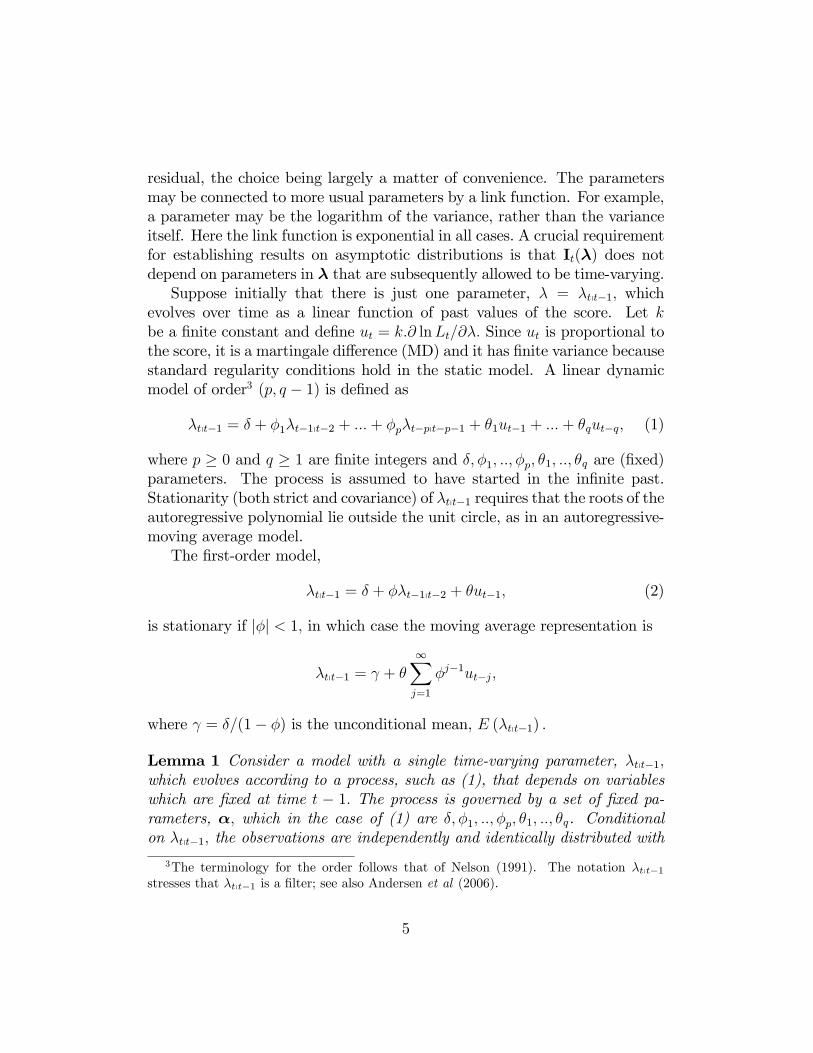
residual, the choice being largely a matter of convenience. The parametersmay be connected to more usual parameters by a link function. For example,a parameter may be the logarithm of the variance, rather than the varianceitself. Here the link function is exponential in all cases. A crucial requirementfor establishing results on asymptotic distributions is that It(�) does notdepend on parameters in � that are subsequently allowed to be time-varying.Suppose initially that there is just one parameter, � = �tpt�1; which

evolves over time as a linear function of past values of the score. Let kbe a �nite constant and de�ne ut = k:@ lnLt=@�: Since ut is proportional tothe score, it is a martingale di¤erence (MD) and it has �nite variance becausestandard regularity conditions hold in the static model. A linear dynamicmodel of order3 (p; q � 1) is de�ned as

�tpt�1 = � + �1�t�1pt�2 + :::+ �p�t�ppt�p�1 + �1ut�1 + :::+ �qut�q; (1)

where p � 0 and q � 1 are �nite integers and �; �1; ::; �p; �1; ::; �q are (�xed)parameters. The process is assumed to have started in the in�nite past.Stationarity (both strict and covariance) of �tpt�1 requires that the roots of theautoregressive polynomial lie outside the unit circle, as in an autoregressive-moving average model.The �rst-order model,

�tpt�1 = � + ��t�1pt�2 + �ut�1; (2)

is stationary if j�j < 1; in which case the moving average representation is

�tpt�1 = + �1Xj=1

�j�1ut�j;

where = �=(1� �) is the unconditional mean, E (�tpt�1) :

Lemma 1 Consider a model with a single time-varying parameter, �tpt�1;which evolves according to a process, such as (1), that depends on variableswhich are �xed at time t � 1: The process is governed by a set of �xed pa-rameters, �; which in the case of (1) are �; �1; ::; �p; �1; ::; �q. Conditionalon �tpt�1; the observations are independently and identically distributed with

3The terminology for the order follows that of Nelson (1991). The notation �tpt�1stresses that �tpt�1 is a �lter; see also Andersen et al (2006).

5

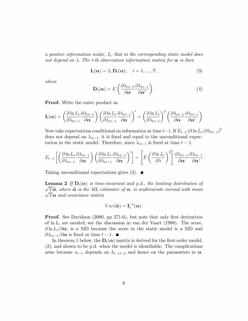
a positive information scalar, It; that in the corresponding static model doesnot depend on �: The t-th observation information matrix for � is then

It(�) = It:Dt(�); t = 1; ::::; T; (3)

where

Dt(�) = E

�@�tpt�1@�

@�tpt�1@�0

�: (4)

Proof. Write the outer product as

It(�) =

�@ lnLt@�tpt�1

@�tpt�1@�

��@ lnLt@�tpt�1

@�tpt�1@�

�0=

�@ lnLt@�tpt�1

�2�@�tpt�1@�

@�tpt�1@�0

�Now take expectations conditional on information at time t�1: IfEt�1 (@ lnLt/@�tpt�1)2does not depend on �tpt�1; it is �xed and equal to the unconditional expec-tation in the static model. Therefore, since �tpt�1 is �xed at time t� 1;

Et�1

��@ lnLt@�tpt�1

@�tpt�1@�

��@ lnLt@�tpt�1

@�tpt�1@�

�0�=

"E

�@ lnLt@�

�2#@�tpt�1@�

@�tpt�1@�0

:

Taking unconditional expectations gives (3).

Lemma 2 If Dt(�) is time-invariant and p.d., the limiting distribution ofpT e�; where e� is the ML estimator of �, is multivariate normal with meanpT� and covariance matrix

V ar(e�) = I�1t (�):Proof. See Davidson (2000, pp 271-6), but note that only �rst derivativesof lnLt are needed; see the discussion in van der Vaart (1998). The score,@ lnLt=@�; is a MD because the score in the static model is a MD and@�tpt�1=@� is �xed at time t� 1:In theorem 1 below, theDt(�) matrix is derived for the �rst-order model,

(2), and shown to be p.d. when the model is identi�able. The complicationsarise because ut�1 depends on �t�1pt�2 and hence on the parameters in �:

6

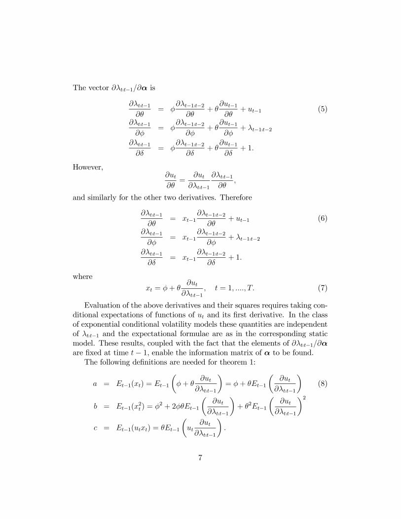
The vector @�tpt�1=@� is

@�tpt�1@�

= �@�t�1pt�2

@�+ �

@ut�1@�

+ ut�1 (5)

@�tpt�1@�

= �@�t�1pt�2@�

+ �@ut�1@�

+ �t�1pt�2

@�tpt�1@�

= �@�t�1pt�2

@�+ �

@ut�1@�

+ 1:

However,@ut@�

=@ut

@�tpt�1

@�tpt�1@�

;

and similarly for the other two derivatives. Therefore

@�tpt�1@�

= xt�1@�t�1pt�2

@�+ ut�1 (6)

@�tpt�1@�

= xt�1@�t�1pt�2@�

+ �t�1pt�2

@�tpt�1@�

= xt�1@�t�1pt�2

@�+ 1:

where

xt = �+ �@ut

@�tpt�1; t = 1; ::::; T: (7)

Evaluation of the above derivatives and their squares requires taking con-ditional expectations of functions of ut and its �rst derivative. In the classof exponential conditional volatility models these quantities are independentof �tpt�1 and the expectational formulae are as in the corresponding staticmodel. These results, coupled with the fact that the elements of @�tpt�1=@�are �xed at time t� 1, enable the information matrix of � to be found.The following de�nitions are needed for theorem 1:

a = Et�1(xt) = Et�1

��+ �

@ut@�tpt�1

�= �+ �Et�1

�@ut

@�tpt�1

�(8)

b = Et�1(x2t ) = �2 + 2��Et�1

�@ut

@�tpt�1

�+ �2Et�1

�@ut

@�tpt�1

�2c = Et�1(utxt) = �Et�1

�ut

@ut@�tpt�1

�:

7

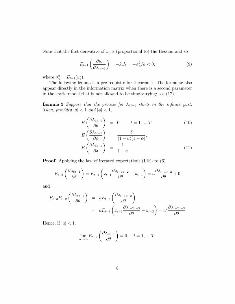
Note that the �rst derivative of ut is (proportional to) the Hessian and so

Et�1

�@ut

@�tpt�1

�= �k:It = ��2u=k < 0; (9)

where �2u = Et�1(u2t ):

The following lemma is a pre-requisite for theorem 1. The formulae alsoappear directly in the information matrix when there is a second parameterin the static model that is not allowed to be time-varying; see (17).

Lemma 3 Suppose that the process for �tpt�1 starts in the in�nite past.Then, provided jaj < 1 and j�j < 1;

E

�@�tpt�1@�

�= 0; t = 1; :::; T; (10)

E

�@�tpt�1@�

�=

�

(1� a)(1� �);

E

�@�tpt�1@�

�=

1

1� a: (11)

Proof. Applying the law of iterated expectations (LIE) to (6)

Et�2

�@�tpt�1@�

�= Et�2

�xt�1

@�t�1pt�2@�

+ ut�1

�= a

@�t�1pt�2@�

+ 0

and

Et�3Et�2

�@�tpt�1@�

�= aEt�3

�@�t�1pt�2

@�

�= aEt�3

�xt�2

@�t�2pt�3@�

+ ut�2

�= a2

@�t�2pt�3@�

Hence, if jaj < 1;

limn!1

Et�n

�@�tpt�1@�

�= 0; t = 1; :::; T:

8

Taking conditional expectations of @�tpt�1=@� at time t� 2 gives

Et�2

�@�tpt�1@�

�= a

@�t�1pt�2@�

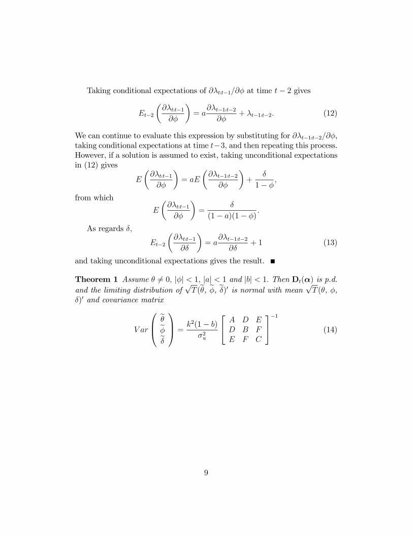
+ �t�1pt�2: (12)

We can continue to evaluate this expression by substituting for @�t�1pt�2=@�,taking conditional expectations at time t�3; and then repeating this process.However, if a solution is assumed to exist, taking unconditional expectationsin (12) gives

E

�@�tpt�1@�

�= aE

�@�t�1pt�2@�

�+

�

1� �;

from which

E

�@�tpt�1@�

�=

�

(1� a)(1� �):

As regards �;

Et�2

�@�tpt�1@�

�= a

@�t�1pt�2@�

+ 1 (13)

and taking unconditional expectations gives the result.

Theorem 1 Assume � 6= 0; j�j < 1; jaj < 1 and jbj < 1: Then Dt(�) is p.d.and the limiting distribution of

pT (e�, e�, e�)0 is normal with mean pT (�, �,

�)0 and covariance matrix

V ar

0B@ e�e�e�1CA =

k2(1� b)

�2u

24 A D ED B FE F C

35�1 (14)

9

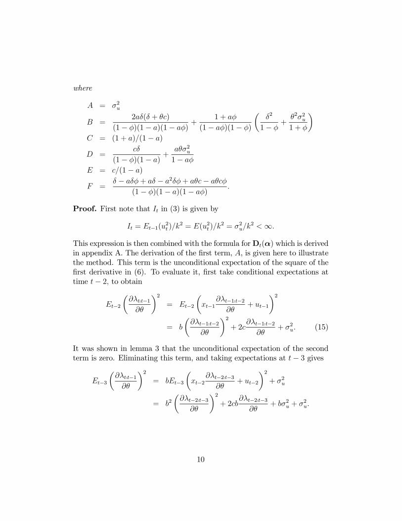
where

A = �2u

B =2a�(� + �c)

(1� �)(1� a)(1� a�)+

1 + a�

(1� a�)(1� �)

��2

1� �+�2�2u1 + �

�C = (1 + a)=(1� a)

D =c�

(1� �)(1� a)+

a��2u1� a�

E = c=(1� a)

F =� � a��+ a� � a2��+ a�c� a�c�

(1� �)(1� a)(1� a�):

Proof. First note that It in (3) is given by

It = Et�1(u2t )=k

2 = E(u2t )=k2 = �2u=k

2 <1:

This expression is then combined with the formula forDt(�) which is derivedin appendix A. The derivation of the �rst term, A, is given here to illustratethe method. This term is the unconditional expectation of the square of the�rst derivative in (6). To evaluate it, �rst take conditional expectations attime t� 2; to obtain

Et�2

�@�tpt�1@�

�2= Et�2

�xt�1

@�t�1pt�2@�

+ ut�1

�2= b

�@�t�1pt�2

@�

�2+ 2c

@�t�1pt�2@�

+ �2u: (15)

It was shown in lemma 3 that the unconditional expectation of the secondterm is zero. Eliminating this term, and taking expectations at t� 3 gives

Et�3

�@�tpt�1@�

�2= bEt�3

�xt�2

@�t�2pt�3@�

+ ut�2

�2+ �2u

= b2�@�t�2pt�3

@�

�2+ 2cb

@�t�2pt�3@�

+ b�2u + �2u:

10

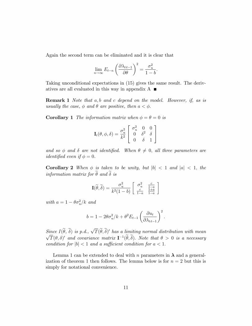
Again the second term can be eliminated and it is clear that

limn!1

Et�n

�@�tpt�1@�

�2=

�2u1� b

:

Taking unconditional expectations in (15) gives the same result. The deriv-atives are all evaluated in this way in appendix A

Remark 1 Note that a; b and c depend on the model. However, if, as isusually the case, � and � are positive, then a < �:

Corollary 1 The information matrix when � = � = 0 is

It(�; �; �) =�2uk2

24 �2u 0 00 �2 �0 � 1

35and so � and � are not identi�ed. When � 6= 0; all three parameters areidenti�ed even if � = 0.

Corollary 2 When � is taken to be unity, but jbj < 1 and jaj < 1; theinformation matrix for e� and e� is

I(e�;e�) = �2uk2(1� b)

��2u

c1�a

c1�a

1+a1�a

�with a = 1� ��2u=k and

b = 1� 2��2u=k + �2Et�1

�@ut

@�tpt�1

�2:

Since I(e�, e�) is p.d., pT (e�;e�)0 has a limiting normal distribution with meanpT (�; �)0 and covariance matrix I�1(e�;e�): Note that � > 0 is a necessary

condition for jbj < 1 and a su¢ cient condition for a < 1:

Lemma 1 can be extended to deal with n parameters in � and a general-ization of theorem 1 then follows. The lemma below is for n = 2 but this issimply for notational convenience.

11

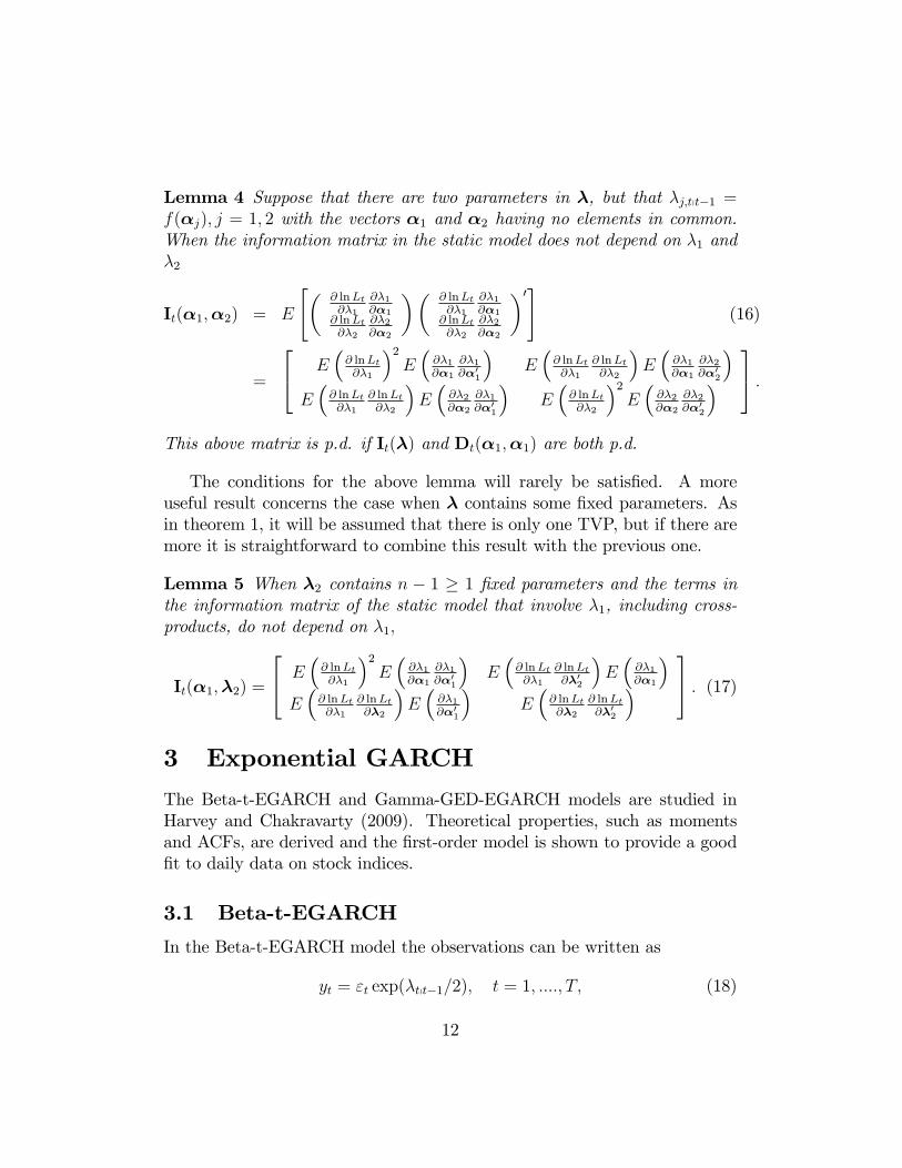
Lemma 4 Suppose that there are two parameters in �, but that �j;tpt�1 =f(�j); j = 1; 2 with the vectors �1 and �2 having no elements in common.When the information matrix in the static model does not depend on �1 and�2

It(�1;�2) = E

"� @ lnLt@�1

@�1@�1

@ lnLt@�2

@�2@�2

�� @ lnLt@�1

@�1@�1

@ lnLt@�2

@�2@�2

�0#(16)

=

24 E�@ lnLt@�1

�2E�@�1@�1

@�1@�01

�E�@ lnLt@�1

@ lnLt@�2

�E�@�1@�1

@�2@�02

�E�@ lnLt@�1

@ lnLt@�2

�E�@�2@�2

@�1@�01

�E�@ lnLt@�2

�2E�@�2@�2

@�2@�02

�35 :

This above matrix is p.d. if It(�) and Dt(�1;�1) are both p.d.

The conditions for the above lemma will rarely be satis�ed. A moreuseful result concerns the case when � contains some �xed parameters. Asin theorem 1, it will be assumed that there is only one TVP, but if there aremore it is straightforward to combine this result with the previous one.

Lemma 5 When �2 contains n � 1 � 1 �xed parameters and the terms inthe information matrix of the static model that involve �1, including cross-products, do not depend on �1;

It(�1;�2) =

24 E�@ lnLt@�1

�2E�@�1@�1

@�1@�01

�E�@ lnLt@�1

@ lnLt@�02

�E�@�1@�1

�E�@ lnLt@�1

@ lnLt@�2

�E�@�1@�01

�E�@ lnLt@�2

@ lnLt@�02

�35 : (17)

3 Exponential GARCH

The Beta-t-EGARCH and Gamma-GED-EGARCH models are studied inHarvey and Chakravarty (2009). Theoretical properties, such as momentsand ACFs, are derived and the �rst-order model is shown to provide a good�t to daily data on stock indices.

3.1 Beta-t-EGARCH

In the Beta-t-EGARCH model the observations can be written as

yt = "t exp(�tpt�1=2); t = 1; ::::; T; (18)

12

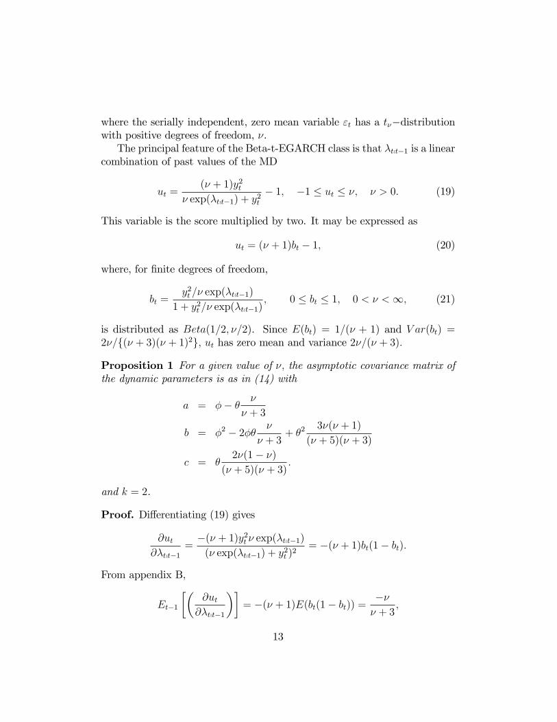
where the serially independent, zero mean variable "t has a t��distributionwith positive degrees of freedom, �.The principal feature of the Beta-t-EGARCH class is that �tpt�1 is a linear

combination of past values of the MD

ut =(� + 1)y2t

� exp(�tpt�1) + y2t� 1; �1 � ut � �; � > 0: (19)

This variable is the score multiplied by two. It may be expressed as

ut = (� + 1)bt � 1; (20)

where, for �nite degrees of freedom,

bt =y2t =� exp(�tpt�1)

1 + y2t =� exp(�tpt�1); 0 � bt � 1; 0 < � <1; (21)

is distributed as Beta(1=2; �=2). Since E(bt) = 1=(� + 1) and V ar(bt) =2�=f(� + 3)(� + 1)2g; ut has zero mean and variance 2�=(� + 3):

Proposition 1 For a given value of �; the asymptotic covariance matrix ofthe dynamic parameters is as in (14) with

a = �� ��

� + 3

b = �2 � 2�� �

� + 3+ �2

3�(� + 1)

(� + 5)(� + 3)

c = �2�(1� �)

(� + 5)(� + 3):

and k = 2.

Proof. Di¤erentiating (19) gives

@ut@�tpt�1

=�(� + 1)y2t � exp(�tpt�1)(� exp(�tpt�1) + y2t )

2= �(� + 1)bt(1� bt):

From appendix B,

Et�1

��@ut

@�tpt�1

��= �(� + 1)E(bt(1� bt)) =

��� + 3

;

13

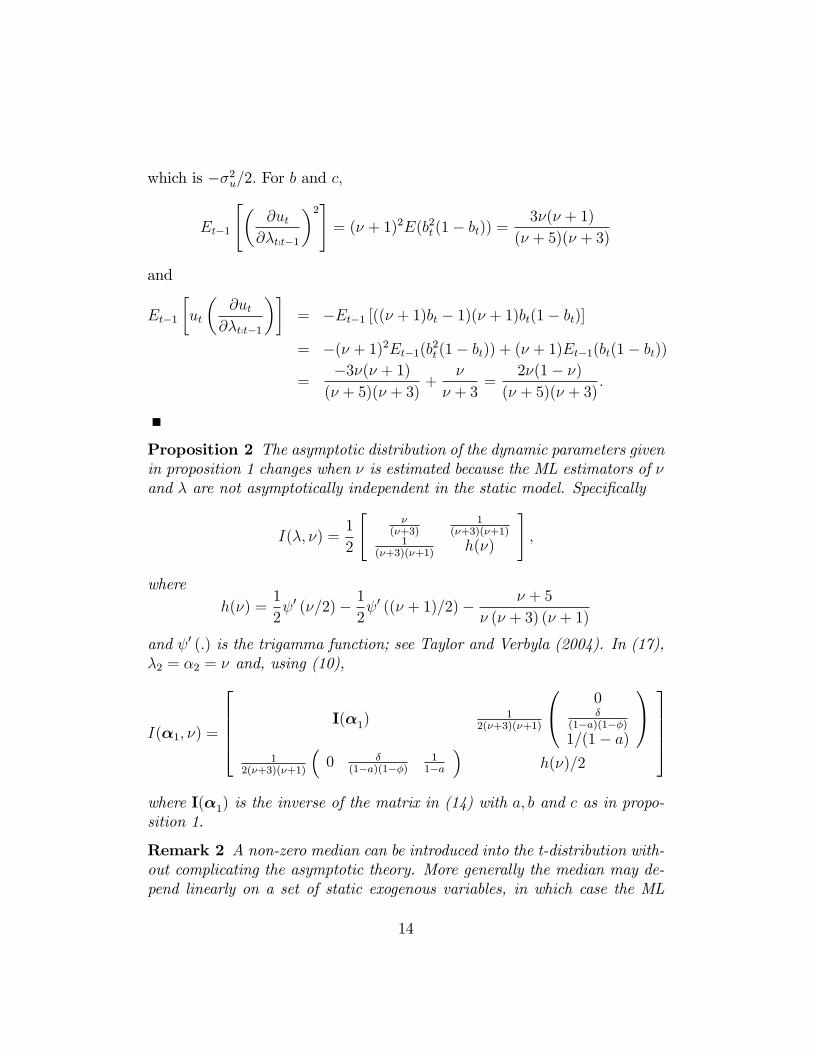
which is ��2u=2: For b and c;

Et�1

"�@ut

@�tpt�1

�2#= (� + 1)2E(b2t (1� bt)) =

3�(� + 1)

(� + 5)(� + 3)

and

Et�1

�ut

�@ut

@�tpt�1

��= �Et�1 [((� + 1)bt � 1)(� + 1)bt(1� bt)]

= �(� + 1)2Et�1(b2t (1� bt)) + (� + 1)Et�1(bt(1� bt))

=�3�(� + 1)(� + 5)(� + 3)

+�

� + 3=

2�(1� �)

(� + 5)(� + 3):

Proposition 2 The asymptotic distribution of the dynamic parameters givenin proposition 1 changes when � is estimated because the ML estimators of �and � are not asymptotically independent in the static model. Speci�cally

I(�; �) =1

2

"�

(�+3)1

(�+3)(�+1)1

(�+3)(�+1)h(�)

#;

whereh(�) =

1

2 0 (�=2)� 1

2 0 ((� + 1)=2)� � + 5

� (� + 3) (� + 1)

and 0 (:) is the trigamma function; see Taylor and Verbyla (2004). In (17),�2 = �2 = � and, using (10),

I(�1; �) =

26664 I(�1)1

2(�+3)(�+1)

0@ 0�

(1�a)(1��)1=(1� a)

1A1

2(�+3)(�+1)

�0 �

(1�a)(1��)11�a

�h(�)=2

37775where I(�1) is the inverse of the matrix in (14) with a; b and c as in propo-sition 1.

Remark 2 A non-zero median can be introduced into the t-distribution with-out complicating the asymptotic theory. More generally the median may de-pend linearly on a set of static exogenous variables, in which case the ML

14

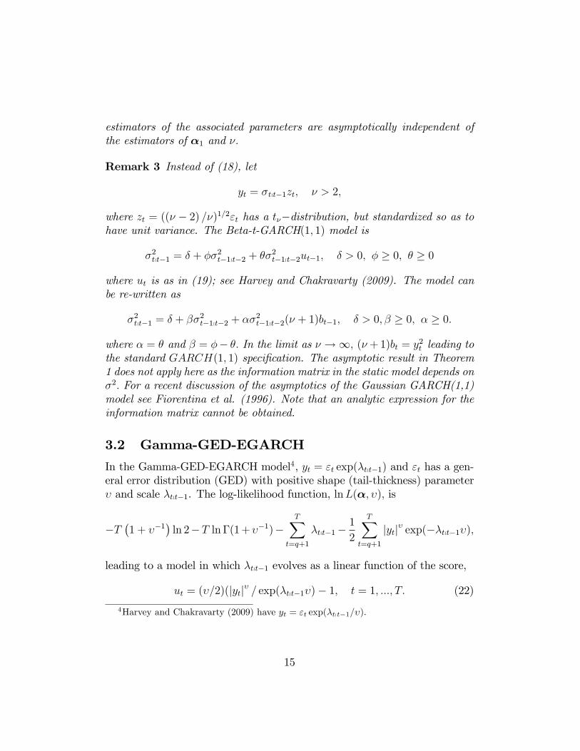
estimators of the associated parameters are asymptotically independent ofthe estimators of �1 and �:

Remark 3 Instead of (18), let

yt = �tpt�1zt; � > 2;

where zt = ((� � 2) =�)1=2"t has a t��distribution, but standardized so as tohave unit variance. The Beta-t-GARCH(1; 1) model is

�2tpt�1 = � + ��2t�1pt�2 + ��2t�1pt�2ut�1; � > 0; � � 0; � � 0

where ut is as in (19); see Harvey and Chakravarty (2009). The model canbe re-written as

�2tpt�1 = � + ��2t�1pt�2 + ��2t�1pt�2(� + 1)bt�1; � > 0; � � 0; � � 0:

where � = � and � = �� �: In the limit as � !1; (� +1)bt = y2t leading tothe standard GARCH(1; 1) speci�cation. The asymptotic result in Theorem1 does not apply here as the information matrix in the static model depends on�2: For a recent discussion of the asymptotics of the Gaussian GARCH(1,1)model see Fiorentina et al. (1996). Note that an analytic expression for theinformation matrix cannot be obtained.

3.2 Gamma-GED-EGARCH

In the Gamma-GED-EGARCH model4, yt = "t exp(�tpt�1) and "t has a gen-eral error distribution (GED) with positive shape (tail-thickness) parameter� and scale �tpt�1. The log-likelihood function, lnL(�; �); is

�T�1 + ��1

�ln 2�T ln �(1+��1)�

TXt=q+1

�tpt�1�1

2

TXt=q+1

jytj� exp(��tpt�1�);

leading to a model in which �tpt�1 evolves as a linear function of the score,

ut = (�=2)(jytj� = exp(�tpt�1�)� 1; t = 1; :::; T: (22)

4Harvey and Chakravarty (2009) have yt = "t exp(�tpt�1=�):

15

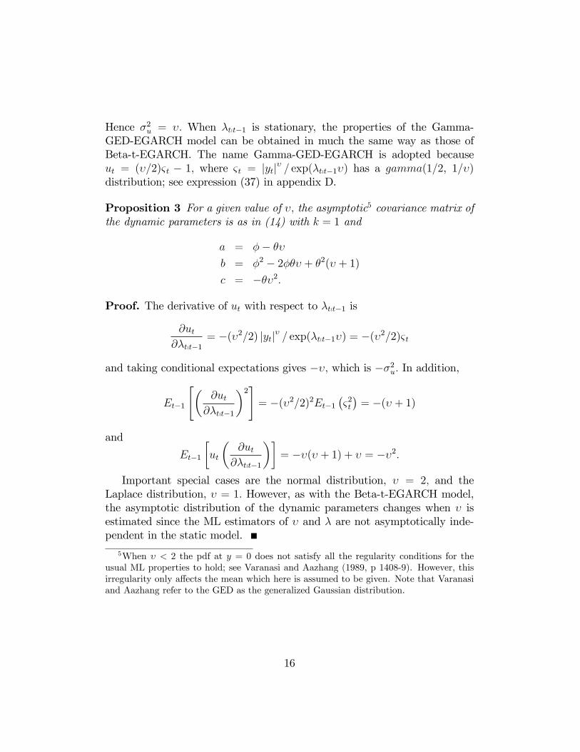
Hence �2u = �: When �tpt�1 is stationary, the properties of the Gamma-GED-EGARCH model can be obtained in much the same way as those ofBeta-t-EGARCH. The name Gamma-GED-EGARCH is adopted becauseut = (�=2)& t � 1; where & t = jytj� = exp(�tpt�1�) has a gamma(1=2, 1=�)distribution; see expression (37) in appendix D.

Proposition 3 For a given value of �; the asymptotic5 covariance matrix ofthe dynamic parameters is as in (14) with k = 1 and

a = �� ��

b = �2 � 2��� + �2(� + 1)

c = ���2:

Proof. The derivative of ut with respect to �tpt�1 is

@ut@�tpt�1

= �(�2=2) jytj� = exp(�tpt�1�) = �(�2=2)& t

and taking conditional expectations gives ��; which is ��2u: In addition,

Et�1

"�@ut

@�tpt�1

�2#= �(�2=2)2Et�1

�&2t�= �(� + 1)

and

Et�1

�ut

�@ut

@�tpt�1

��= ��(� + 1) + � = ��2:

Important special cases are the normal distribution, � = 2; and theLaplace distribution, � = 1: However, as with the Beta-t-EGARCH model,the asymptotic distribution of the dynamic parameters changes when � isestimated since the ML estimators of � and � are not asymptotically inde-pendent in the static model.

5When � < 2 the pdf at y = 0 does not satisfy all the regularity conditions for theusual ML properties to hold; see Varanasi and Aazhang (1989, p 1408-9). However, thisirregularity only a¤ects the mean which here is assumed to be given. Note that Varanasiand Aazhang refer to the GED as the generalized Gaussian distribution.

16

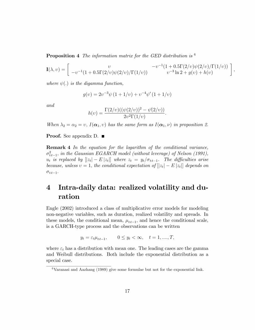
Proposition 4 The information matrix for the GED distribution is 6

I(�; �) =

�� ���1(1 + 0:5�(2=�) (2=�)=�(1=�))

���1(1 + 0:5�(2=�) (2=�)=�(1=�)) ��3 ln 2 + g(�) + h(�)

�;

where (:) is the digamma function,

g(�) = 2��3 (1 + 1=�) + ��4 0 (1 + 1=�)

and

h(�) =�(2=�)(( (2=�))2 � �(2=�))

2�2�(1=�):

When �2 = �2 = �; I(�1; �) has the same form as I(�1; �) in proposition 2.

Proof. See appendix D.

Remark 4 In the equation for the logarithm of the conditional variance,�2tpt�1; in the Gaussian EGARCH model (without leverage) of Nelson (1991),ut is replaced by [jztj � E jztj] where zt = yt=�tpt�1. The di¢ culties arisebecause, unless � = 1; the conditional expectation of [jztj � E jztj] depends on�tpt�1:

4 Intra-daily data: realized volatility and du-ration

Engle (2002) introduced a class of multiplicative error models for modelingnon-negative variables, such as duration, realized volatility and spreads. Inthese models, the conditional mean, �tpt�1; and hence the conditional scale,is a GARCH-type process and the observations can be written

yt = "t�tpt�1; 0 � yt <1; t = 1; ::::; T;

where "t has a distribution with mean one. The leading cases are the gammaand Weibull distributions. Both include the exponential distribution as aspecial case.

6Varanasi and Aazhang (1989) give some formulae but not for the exponential link.

17

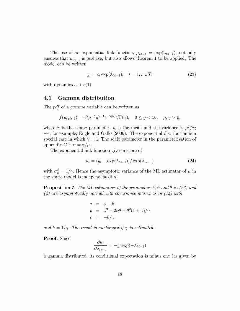
The use of an exponential link function, �tpt�1 = exp(�tpt�1); not onlyensures that �tpt�1 is positive, but also allows theorem 1 to be applied. Themodel can be written

yt = "t exp(�tpt�1); t = 1; ::::; T; (23)

with dynamics as in (1).

4.1 Gamma distribution

The pdf of a gamma variable can be written as

f(y;�; ) = �� y �1e� y=�=�( ); 0 � y <1; �; > 0;

where is the shape parameter, � is the mean and the variance is �2= ;see, for example, Engle and Gallo (2006). The exponential distribution is aspecial case in which = 1: The scale parameter in the parameterization ofappendix C is � = =�:The exponential link function gives a score of

ut = (yt � exp(�tpt�1))= exp(�tpt�1) (24)

with �2u = 1= : Hence the asymptotic variance of the ML estimator of � inthe static model is independent of �:

Proposition 5 The ML estimators of the parameters �; � and � in (23) and(2) are asymptotically normal with covariance matrix as in (14) with

a = �� �

b = �2 � 2�� + �2(1 + )=

c = ��=

and k = 1= : The result is unchanged if is estimated.

Proof. Since@ut

@�tpt�1= �yt exp(��tpt�1)

is gamma distributed, its conditional expectation is minus one (as given by

18

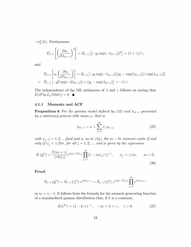
��2u=k). Furthermore

Et�1

"�@ut

@�tpt�1

�2#= Et�1

�(�yt exp(��tpt�1))2

�= (1 + )= ;

and

Et�1

�ut

�@ut

@�tpt�1

��= Et�1 [�yt exp(��tpt�1)((yt � exp(�tpt�1))= exp(�tpt�1))]

= Et�1��y2t exp(�2�tpt�1)) + (yt � exp(�tpt�1)

�= �1= :

The independence of the ML estimators of � and follows on noting thatE(@2 lnLt=@�@ ) = 0:

4.1.1 Moments and ACF

Proposition 6 For the gamma model de�ned by (23) and �tpt�1 generatedby a stationary process with mean !; that is

�tpt�1 = ! +1Xj=1

jut�j; (25)

with j; j = 1; 2; :: �xed and ut as in (24), the m� th moment exists if andonly if j < =2m; for all j = 1; 2; :::; and is given by the expression

E (ymt ) =�(m+ )

m�( )em(!�� j)

1Yj=1

(1�m j= )� ; j < =m; m > 0:

(26)

Proof.

Et�1 (ymt ) = Et�1 ("

mt ) :e

m�tpt�1 = Et�1 ("mt ) :e

m(!�� j)1Yj=1

em j"t�j

as ut = "t�1: It follows from the formula for the moment generating functionof a standardized gamma distribution that, if k is a constant,

E(ek") = (1� k= )� ; �1 < k < ; > 0: (27)

19

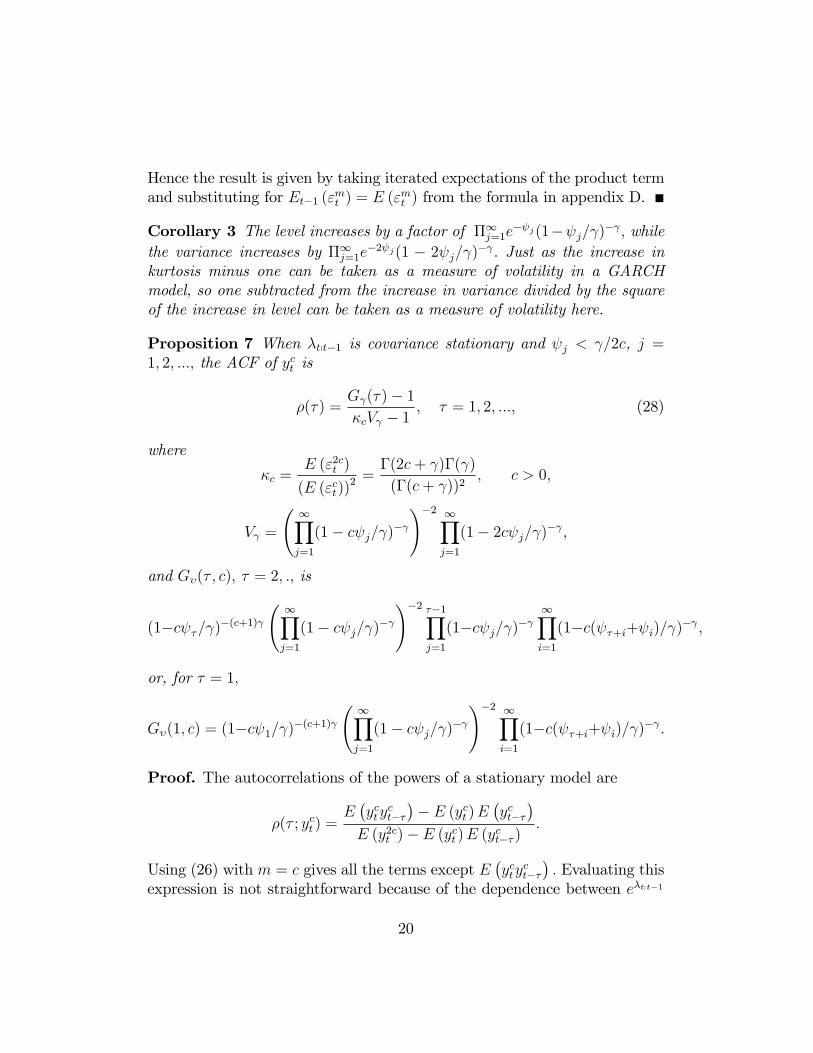
Hence the result is given by taking iterated expectations of the product termand substituting for Et�1 ("mt ) = E ("mt ) from the formula in appendix D.

Corollary 3 The level increases by a factor of �1j=1e� j(1� j= )� ; while

the variance increases by �1j=1e�2 j(1 � 2 j= )� : Just as the increase in

kurtosis minus one can be taken as a measure of volatility in a GARCHmodel, so one subtracted from the increase in variance divided by the squareof the increase in level can be taken as a measure of volatility here.

Proposition 7 When �tpt�1 is covariance stationary and j < =2c, j =1; 2; :::; the ACF of yct is

�(�) =G (�)� 1�cV � 1

; � = 1; 2; :::; (28)

where

�c =E ("2ct )

(E ("ct))2 =

�(2c+ )�( )

(�(c+ ))2; c > 0;

V =

1Yj=1

(1� c j= )�

!�2 1Yj=1

(1� 2c j= )� ;

and G�(� ; c); � = 2; :; is

(1�c �= )�(c+1) 1Yj=1

(1� c j= )�

!�2 ��1Yj=1

(1�c j= )� 1Yi=1

(1�c( �+i+ i)= )� ;

or, for � = 1;

G�(1; c) = (1�c 1= )�(c+1) 1Yj=1

(1� c j= )�

!�2 1Yi=1

(1�c( �+i+ i)= )� :

Proof. The autocorrelations of the powers of a stationary model are

�(� ; yct ) =E�ycty

ct���� E (yct )E

�yct��

�E (y2ct )� E (yct )E (y

ct�� )

:

Using (26) with m = c gives all the terms except E�ycty

ct���: Evaluating this

expression is not straightforward because of the dependence between e�tpt�1

20

and "ct�� : Following the argument in Harvey and Chakravarty (2009) givesthe result.The autocorrelations for ln yt; which corresponds to c = 0, are easily

derived because ln yt = �tpt�1 + ln "t:

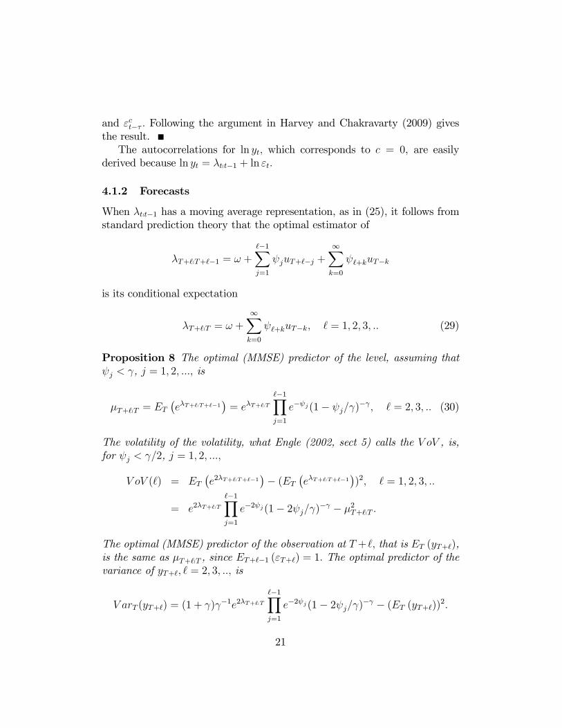
4.1.2 Forecasts

When �tpt�1 has a moving average representation, as in (25), it follows fromstandard prediction theory that the optimal estimator of

�T+`pT+`�1 = ! +`�1Xj=1

juT+`�j +1Xk=0

`+kuT�k

is its conditional expectation

�T+`pT = ! +1Xk=0

`+kuT�k; ` = 1; 2; 3; :: (29)

Proposition 8 The optimal (MMSE) predictor of the level, assuming that j < , j = 1; 2; :::; is

�T+`pT = ET�e�T+`pT+`�1

�= e�T+`pT

`�1Yj=1

e� j(1� j= )� ; ` = 2; 3; :: (30)

The volatility of the volatility, what Engle (2002, sect 5) calls the V oV , is,for j < =2, j = 1; 2; :::;

V oV (`) = ET�e2�T+`pT+`�1

�� (ET

�e�T+`pT+`�1

�)2; ` = 1; 2; 3; ::

= e2�T+`pT`�1Yj=1

e�2 j(1� 2 j= )� � �2T+`pT :

The optimal (MMSE) predictor of the observation at T +`; that is ET (yT+`),is the same as �T+`pT , since ET+`�1 ("T+`) = 1: The optimal predictor of thevariance of yT+`; ` = 2; 3; ::; is

V arT (yT+`) = (1 + ) �1e2�T+`pT

`�1Yj=1

e�2 j(1� 2 j= )� � (ET (yT+`))2:

21

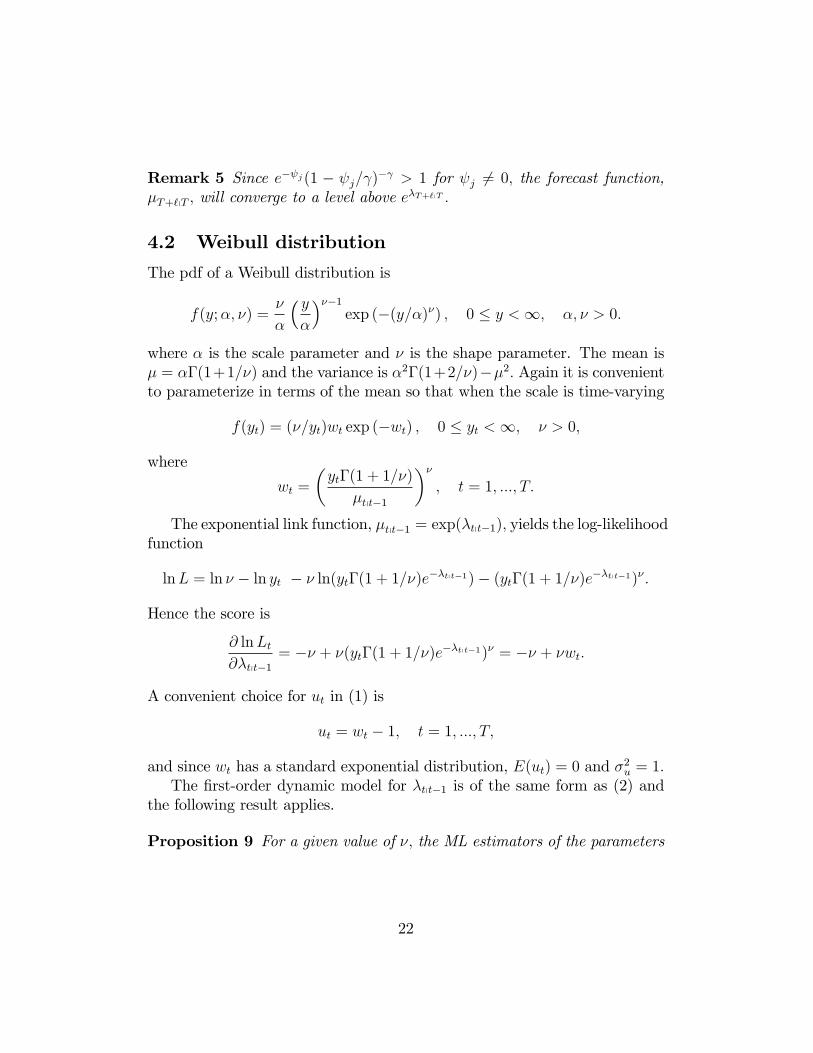
Remark 5 Since e� j(1 � j= )� > 1 for j 6= 0; the forecast function,

�T+`pT ; will converge to a level above e�T+`pT :

4.2 Weibull distribution

The pdf of a Weibull distribution is

f(y;�; �) =�

�

� y�

���1exp (�(y=�)�) ; 0 � y <1; �; � > 0:

where � is the scale parameter and � is the shape parameter. The mean is� = ��(1+1=�) and the variance is �2�(1+2=�)��2: Again it is convenientto parameterize in terms of the mean so that when the scale is time-varying

f(yt) = (�=yt)wt exp (�wt) ; 0 � yt <1; � > 0;

where

wt =

�yt�(1 + 1=�)

�tpt�1

��; t = 1; :::; T:

The exponential link function, �tpt�1 = exp(�tpt�1); yields the log-likelihoodfunction

lnL = ln � � ln yt � � ln(yt�(1 + 1=�)e��tpt�1)� (yt�(1 + 1=�)e��tpt�1)� :

Hence the score is

@ lnLt@�tpt�1

= �� + �(yt�(1 + 1=�)e��tpt�1)� = �� + �wt:

A convenient choice for ut in (1) is

ut = wt � 1; t = 1; :::; T;

and since wt has a standard exponential distribution, E(ut) = 0 and �2u = 1:The �rst-order dynamic model for �tpt�1 is of the same form as (2) and

the following result applies.

Proposition 9 For a given value of �; the ML estimators of the parameters

22

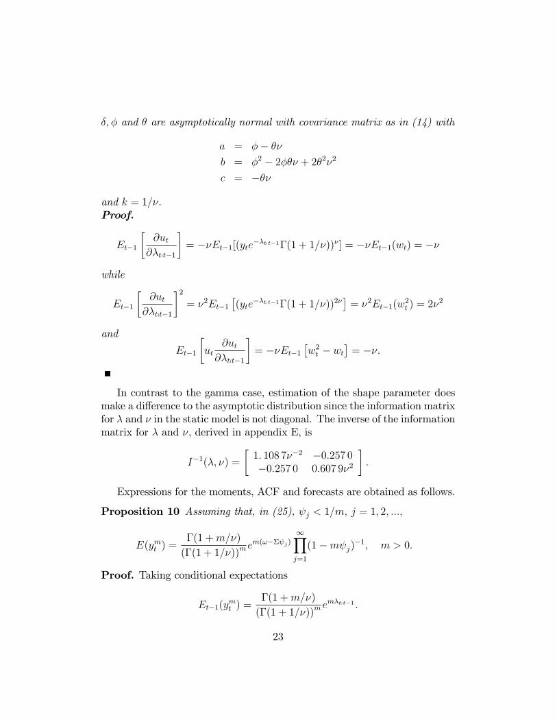
�; � and � are asymptotically normal with covariance matrix as in (14) with

a = �� ��

b = �2 � 2��� + 2�2�2

c = ���

and k = 1=�:Proof.

Et�1

�@ut

@�tpt�1

�= ��Et�1[(yte��tpt�1�(1 + 1=�))� ] = ��Et�1(wt) = ��

while

Et�1

�@ut

@�tpt�1

�2= �2Et�1

�(yte

��tpt�1�(1 + 1=�))2��= �2Et�1(w

2t ) = 2�

2

and

Et�1

�ut

@ut@�tpt�1

�= ��Et�1

�w2t � wt

�= ��:

In contrast to the gamma case, estimation of the shape parameter doesmake a di¤erence to the asymptotic distribution since the information matrixfor � and � in the static model is not diagonal. The inverse of the informationmatrix for � and �, derived in appendix E, is

I�1(�; �) =

�1: 108 7��2 �0:257 0�0:257 0 0:607 9�2

�:

Expressions for the moments, ACF and forecasts are obtained as follows.

Proposition 10 Assuming that, in (25), j < 1=m; j = 1; 2; :::;

E(ymt ) =�(1 +m=�)

(�(1 + 1=�))mem(!�� j)

1Yj=1

(1�m j)�1; m > 0:

Proof. Taking conditional expectations

Et�1(ymt ) =

�(1 +m=�)

(�(1 + 1=�))mem�tpt�1 :

23

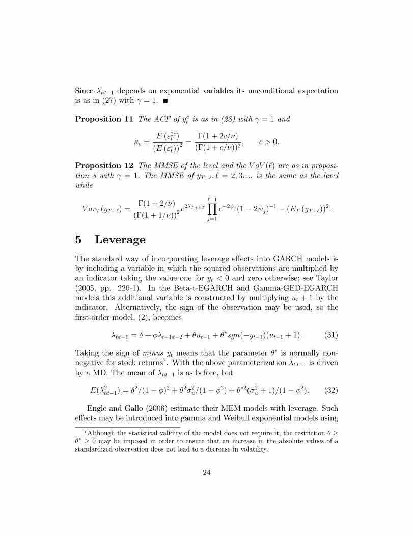
Since �tpt�1 depends on exponential variables its unconditional expectationis as in (27) with = 1:

Proposition 11 The ACF of yct is as in (28) with = 1 and

�c =E ("2ct )

(E ("ct))2 =

�(1 + 2c=�)

(�(1 + c=�))2; c > 0:

Proposition 12 The MMSE of the level and the V oV (`) are as in proposi-tion 8 with = 1: The MMSE of yT+`; ` = 2; 3; ::; is the same as the levelwhile

V arT (yT+`) =�(1 + 2=�)

(�(1 + 1=�))2e2�T+`pT

`�1Yj=1

e�2 j(1� 2 j)�1 � (ET (yT+`))2:

5 Leverage

The standard way of incorporating leverage e¤ects into GARCH models isby including a variable in which the squared observations are multiplied byan indicator taking the value one for yt < 0 and zero otherwise; see Taylor(2005, pp. 220-1). In the Beta-t-EGARCH and Gamma-GED-EGARCHmodels this additional variable is constructed by multiplying ut + 1 by theindicator. Alternatively, the sign of the observation may be used, so the�rst-order model, (2), becomes

�tpt�1 = � + ��t�1pt�2 + �ut�1 + ��sgn(�yt�1)(ut�1 + 1): (31)

Taking the sign of minus yt means that the parameter �� is normally non-

negative for stock returns7. With the above parameterization �tpt�1 is drivenby a MD. The mean of �tpt�1 is as before, but

E(�2tpt�1) = �2=(1� �)2 + �2�2u=(1� �2) + ��2(�2u + 1)=(1� �2): (32)

Engle and Gallo (2006) estimate their MEM models with leverage. Suche¤ects may be introduced into gamma and Weibull exponential models using

7Although the statistical validity of the model does not require it, the restriction � ��� � 0 may be imposed in order to ensure that an increase in the absolute values of astandardized observation does not lead to a decrease in volatility.

24

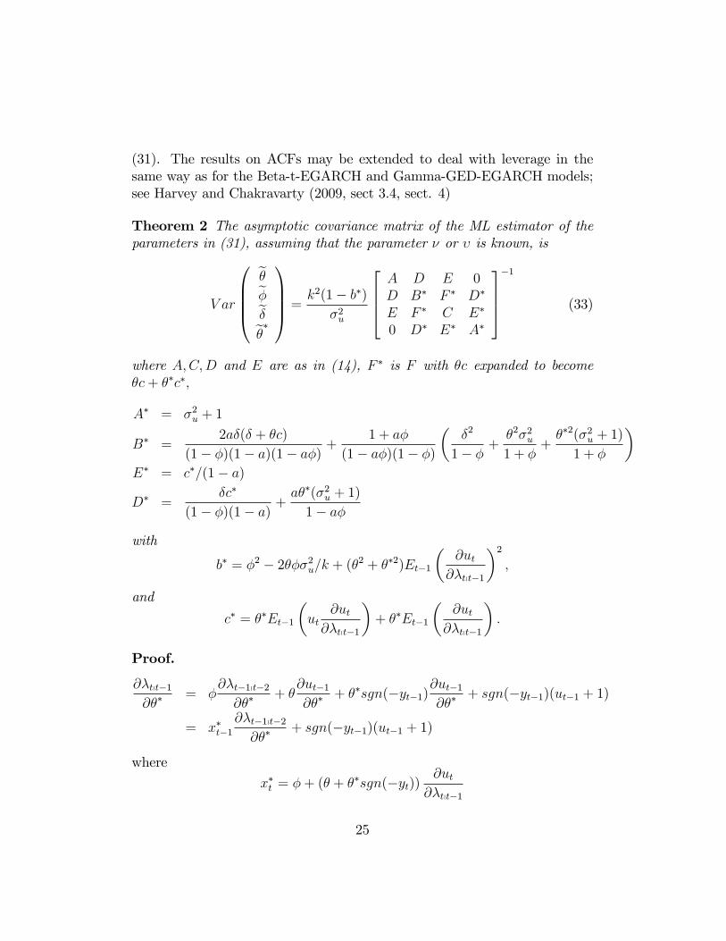
(31). The results on ACFs may be extended to deal with leverage in thesame way as for the Beta-t-EGARCH and Gamma-GED-EGARCH models;see Harvey and Chakravarty (2009, sect 3.4, sect. 4)

Theorem 2 The asymptotic covariance matrix of the ML estimator of theparameters in (31), assuming that the parameter � or � is known, is

V ar

0BBB@e�e�e�e��1CCCA =

k2(1� b�)

�2u

2664A D E 0D B� F � D�

E F � C E�

0 D� E� A�

3775�1

(33)

where A;C;D and E are as in (14), F � is F with �c expanded to become�c+ ��c�;

A� = �2u + 1

B� =2a�(� + �c)

(1� �)(1� a)(1� a�)+

1 + a�

(1� a�)(1� �)

��2

1� �+�2�2u1 + �

+��2(�2u + 1)

1 + �

�E� = c�=(1� a)

D� =�c�

(1� �)(1� a)+a��(�2u + 1)

1� a�

with

b� = �2 � 2���2u=k + (�2 + ��2)Et�1

�@ut

@�tpt�1

�2;

and

c� = ��Et�1

�ut

@ut@�tpt�1

�+ ��Et�1

�@ut

@�tpt�1

�:

Proof.

@�tpt�1@��

= �@�t�1pt�2@��

+ �@ut�1@��

+ ��sgn(�yt�1)@ut�1@��

+ sgn(�yt�1)(ut�1 + 1)

= x�t�1@�t�1pt�2@��

+ sgn(�yt�1)(ut�1 + 1)

where

x�t = �+ (� + ��sgn(�yt))@ut

@�tpt�1

25

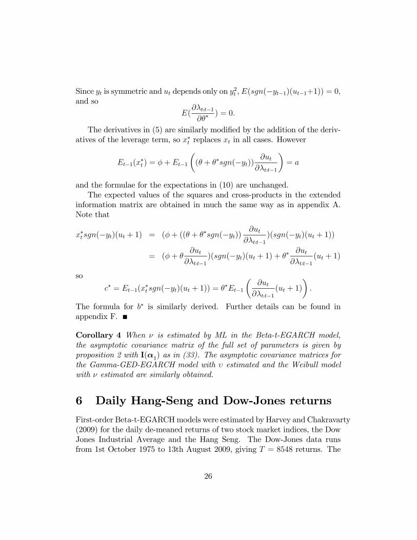
Since yt is symmetric and ut depends only on y2t , E(sgn(�yt�1)(ut�1+1)) = 0;and so

E(@�tpt�1@��

) = 0:

The derivatives in (5) are similarly modi�ed by the addition of the deriv-atives of the leverage term, so x�t replaces xt in all cases. However

Et�1(x�t ) = �+ Et�1

�(� + ��sgn(�yt))

@ut@�tpt�1

�= a

and the formulae for the expectations in (10) are unchanged.The expected values of the squares and cross-products in the extended

information matrix are obtained in much the same way as in appendix A.Note that

x�t sgn(�yt)(ut + 1) = (�+ ((� + ��sgn(�yt))@ut

@�tpt�1)(sgn(�yt)(ut + 1))

= (�+ �@ut

@�tpt�1)(sgn(�yt)(ut + 1) + ��

@ut@�tpt�1

(ut + 1)

so

c� = Et�1(x�t sgn(�yt)(ut + 1)) = ��Et�1

�@ut

@�tpt�1(ut + 1)

�:

The formula for b� is similarly derived. Further details can be found inappendix F.

Corollary 4 When � is estimated by ML in the Beta-t-EGARCH model,the asymptotic covariance matrix of the full set of parameters is given byproposition 2 with I(�1) as in (33). The asymptotic covariance matrices forthe Gamma-GED-EGARCH model with � estimated and the Weibull modelwith � estimated are similarly obtained.

6 Daily Hang-Seng and Dow-Jones returns

First-order Beta-t-EGARCHmodels were estimated by Harvey and Chakravarty(2009) for the daily de-meaned returns of two stock market indices, the DowJones Industrial Average and the Hang Seng. The Dow-Jones data runsfrom 1st October 1975 to 13th August 2009, giving T = 8548 returns. The

26

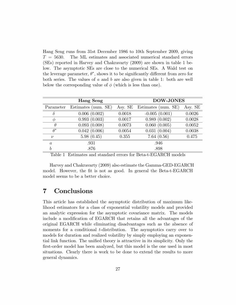
Hang Seng runs from 31st December 1986 to 10th September 2009, givingT = 5630. The ML estimates and associated numerical standard errors(SEs) reported in Harvey and Chakravarty (2009) are shown in table 1 be-low. The asymptotic SEs are close to the numerical SEs. A Wald test onthe leverage parameter, ��; shows it to be signi�cantly di¤erent from zero forboth series. The values of a and b are also given in table 1: both are wellbelow the corresponding value of � (which is less than one).

Hang Seng DOW-JONESParameter Estimates (num. SE) Asy. SE Estimates (num. SE) Asy. SE

� 0.006 (0.002) 0.0018 -0.005 (0.001) 0.0026� 0.993 (0.003) 0.0017 0.989 (0.002) 0.0028� 0.093 (0.008) 0.0073 0.060 (0.005) 0.0052�� 0.042 (0.006) 0.0054 0.031 (0.004) 0.0038� 5.98 (0.45) 0.355 7.64 (0.56) 0.475a .931 .946b .876 .898Table 1 Estimates and standard errors for Beta-t-EGARCH models

Harvey and Chakravarty (2009) also estimate the Gamma-GED-EGARCHmodel. However, the �t is not as good. In general the Beta-t-EGARCHmodel seems to be a better choice.

7 Conclusions

This article has established the asymptotic distribution of maximum like-lihood estimators for a class of exponential volatility models and providedan analytic expression for the asymptotic covariance matrix. The modelsinclude a modi�cation of EGARCH that retains all the advantages of theoriginal EGARCH while eliminating disadvantages such as the absence ofmoments for a conditional t-distribution. The asymptotics carry over tomodels for duration and realized volatility by simply employing an exponen-tial link function. The uni�ed theory is attractive in its simplicity. Only the�rst-order model has been analyzed, but this model is the one used in mostsituations. Clearly there is work to be done to extend the results to moregeneral dynamics.

27

The analysis shows that stationarity of the (�rst-order) dynamic equationis not su¢ cient for the asymptotic theory to be valid. However, it will besu¢ cient in most situations and the other conditions are easily checked. Ifa unit root is imposed on the dynamic equation the asymptotic theory canstill be established.A key feature of the model formulation is that the dynamics are driven

by the score. The associated Lagrange multiplier portmanteau tests for thepresence of volatility similarly depend on residuals derived from the score.The properties of such tests are currently under investigation. The resid-uals derived from the Beta-t-EGARCH model have the advantage of beingmore robust to outliers than tests based on squares, or even absolute values,and this property may well translate into increased power in many practicalsituations.The analytic expression obtained for the information matrix establishes

that it is positive de�nite. This is crucial in demonstrating the validity ofthe asymptotic distribution of the ML estimators. In practice, numericalderivatives may be used for computing ML estimates and at present this isnecessary for higher order models. However, the analytic information ma-trix for the �rst-order model may be of value in enabling ML estimates tobe computed rapidly, by the method of scoring, as well as in providing ac-curate estimates of asymptotic standard errors; see the comments made byFiorentini et al (1996) in the context of GARCH estimation.When observations are from a Gamma�GED-EGARCH model, the stan-

dardized observations, yt exp(��tpt�1); have a gamma(1=2; 1=�) distributionwhen their absolute values are raised to the power �: This link suggests a ra-tionale for using the gamma distribution for certain types of non-negative ob-servations, for example those derived from squares or absolute values. Giventhe attractions of Beta-t-EGARCH and the fact that t2� = F1;� , a model fornon-negative observations in which "t in (23) is distributed as F1;� may beworthy of consideration. In other words if a variable is similar to the squareof an observation from Beta-t-EGARCH, a conditional F1;� is appropriate.More generally "t may be modeled as an F-distribution with (�1; �2) degreesof freedom. The score has a beta distribution8 and theorem 1 still applies.The theory for deriving moments, ACFs and forecasts is similar to that forBeta-t-EGARCH. Although the argument from squaring Beta-t-EGARCH

8For an F (�1; �2) distribution, the score is (�1 + �2)bt=2 � �1=2; where bt has abeta(�1=2; �2=2) distribution.

28

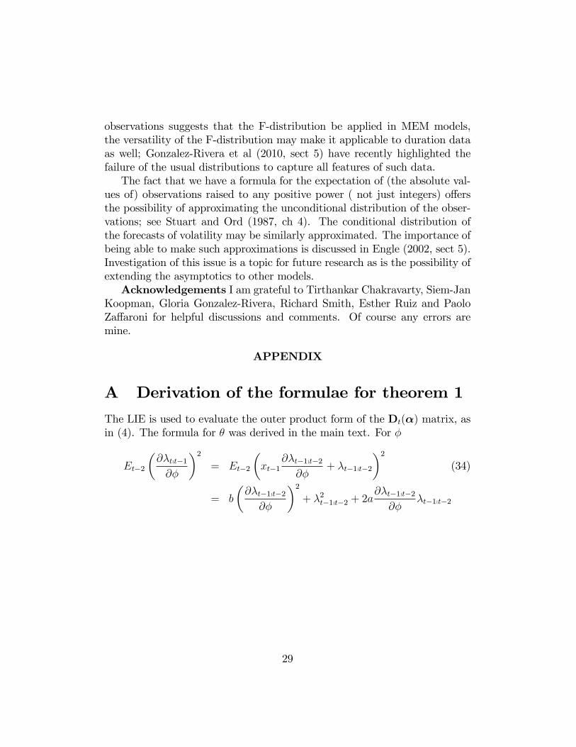
observations suggests that the F-distribution be applied in MEM models,the versatility of the F-distribution may make it applicable to duration dataas well; Gonzalez-Rivera et al (2010, sect 5) have recently highlighted thefailure of the usual distributions to capture all features of such data.The fact that we have a formula for the expectation of (the absolute val-

ues of) observations raised to any positive power ( not just integers) o¤ersthe possibility of approximating the unconditional distribution of the obser-vations; see Stuart and Ord (1987, ch 4). The conditional distribution ofthe forecasts of volatility may be similarly approximated. The importance ofbeing able to make such approximations is discussed in Engle (2002, sect 5).Investigation of this issue is a topic for future research as is the possibility ofextending the asymptotics to other models.Acknowledgements I am grateful to Tirthankar Chakravarty, Siem-Jan

Koopman, Gloria Gonzalez-Rivera, Richard Smith, Esther Ruiz and PaoloZa¤aroni for helpful discussions and comments. Of course any errors aremine.

APPENDIX

A Derivation of the formulae for theorem 1

The LIE is used to evaluate the outer product form of the Dt(�) matrix, asin (4). The formula for � was derived in the main text. For �

Et�2

�@�tpt�1@�

�2= Et�2

�xt�1

@�t�1pt�2@�

+ �t�1pt�2

�2(34)

= b

�@�t�1pt�2@�

�2+ �2t�1pt�2 + 2a

@�t�1pt�2@�

�t�1pt�2

29

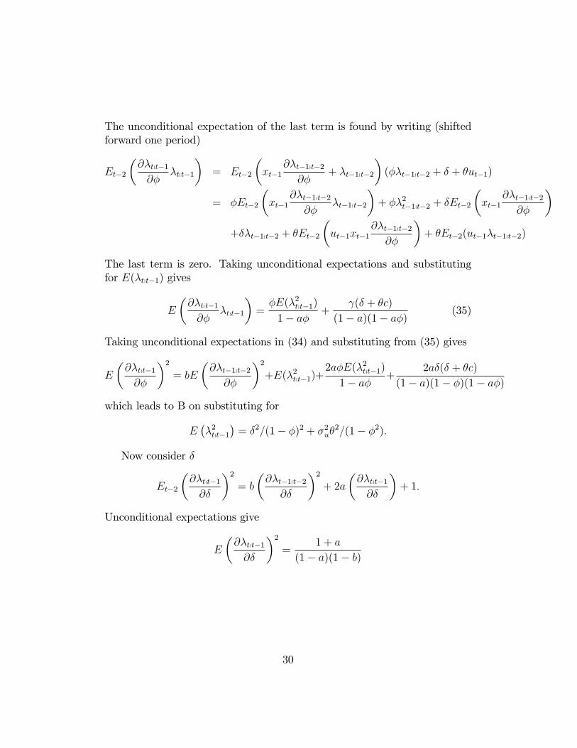
The unconditional expectation of the last term is found by writing (shiftedforward one period)

Et�2

�@�tpt�1@�

�tpt�1

�= Et�2

�xt�1

@�t�1pt�2@�

+ �t�1pt�2

�(��t�1pt�2 + � + �ut�1)

= �Et�2

�xt�1

@�t�1pt�2@�

�t�1pt�2

�+ ��2t�1pt�2 + �Et�2

�xt�1

@�t�1pt�2@�

�+��t�1pt�2 + �Et�2

�ut�1xt�1

@�t�1pt�2@�

�+ �Et�2(ut�1�t�1pt�2)

The last term is zero. Taking unconditional expectations and substitutingfor E(�tpt�1) gives

E

�@�tpt�1@�

�tpt�1

�=�E(�2tpt�1)

1� a�+

(� + �c)

(1� a)(1� a�)(35)

Taking unconditional expectations in (34) and substituting from (35) gives

E

�@�tpt�1@�

�2= bE

�@�t�1pt�2@�

�2+E(�2tpt�1)+

2a�E(�2tpt�1)

1� a�+

2a�(� + �c)

(1� a)(1� �)(1� a�)

which leads to B on substituting for

E��2tpt�1

�= �2=(1� �)2 + �2u�

2=(1� �2):

Now consider �

Et�2

�@�tpt�1@�

�2= b

�@�t�1pt�2

@�

�2+ 2a

�@�tpt�1@�

�+ 1:

Unconditional expectations give

E

�@�tpt�1@�

�2=

1 + a

(1� a)(1� b)

30

As regards the cross-products

Et�2

�@�tpt�1@�

@�tpt�1@�

�= Et�2

��xt�1

@�t�1pt�2@�

+ ut�1

��xt�1

@�t�1pt�2@�

+ �t�1pt�2

��= Et�2

�x2t�1

@�t�1pt�2@�

@�t�1pt�2@�

�+ Et�2

��xt�1ut�1

@�t�1pt�2@�

��+Et�2

��xt�1

@�t�1pt�2@�

�t�1pt�2

��+ Et�2 [�t�1pt�2ut�1]

= b

�@�t�1pt�2

@�

@�t�1pt�2@�

�+ c

@�t�1pt�2@�

+ a

�@�t�1pt�2

@��t�1pt�2

�+ 0

The unconditional expectation of the last (non-zero) term is found by writing(shifted forward one period)

Et�2

�@�tpt�1@�

�tpt�1

�= Et�2

��xt�1

@�t�1pt�2@�

+ ut�1

�(��t�1pt�2 + � + �ut�1)

�= a�E

�@�t�1pt�2

@��t�1pt�2

�+ ��2u

Thus

E

�@�tpt�1@�

�tpt�1

�=

��2u1� a�

leading to D.

Et�2

�@�tpt�1@�

@�tpt�1@�

�= Et�2

��xt�1

@�t�1pt�2@�

+ 1

��xt�1

@�t�1pt�2@�

+ �t�1pt�2

��= b

�@�t�1pt�2

@�

@�t�1pt�2@�

�+ �t�1pt�2 + a

@�t�1pt�2@�

+ a@�t�1pt�2

@��t�1pt�2

For � and �; taking unconditional expectations gives

E

�@�tpt�1@�

@�tpt�1@�

�= bE

�@�t�1pt�2

@�

@�t�1pt�2@�

�+ +

a

1� a+aE

�@�t�1pt�2

@��t�1pt�2

�(36)

31

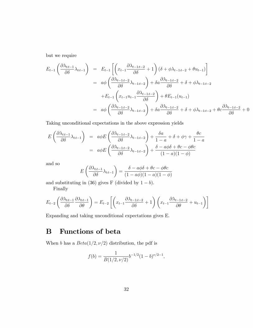
but we require

Et�1

�@�tpt�1@�

�tpt�1

�= Et�1

��xt�1

@�t�1pt�2@�

+ 1

�(� + ��t�1pt�2 + �ut�1)

�= a�

�@�t�1pt�2

@��t�1pt�2

�+ �a

@�t�1pt�2@�

+ � + ��t�1pt�2

+Et�1

�xt�1ut�1

@�t�1pt�2@�

�+ �Et�1(ut�1)

= a�

�@�t�1pt�2

@��t�1pt�2

�+ �a

@�t�1pt�2@�

+ � + ��t�1pt�2 + �c@�t�1pt�2

@�+ 0

Taking unconditional expectations in the above expression yields

E

�@�tpt�1@�

�tpt�1

�= a�E

�@�t�1pt�2

@��t�1pt�2

�+

�a

1� a+ � + � +

�c

1� a

= a�E

�@�t�1pt�2

@��t�1pt�2

�+� � a�� + �c� ��c

(1� a)(1� �)

and so

E

�@�tpt�1@�

�tpt�1

�=

� � a�� + �c� ��c

(1� a�)(1� a)(1� �)

and substituting in (36) gives F (divided by 1� b).Finally

Et�2

�@�tpt�1@�

@�tpt�1@�

�= Et�2

��xt�1

@�t�1pt�2@�

+ 1

��xt�1

@�t�1pt�2@�

+ ut�1

��Expanding and taking unconditional expectations gives E.

B Functions of beta

When b has a Beta(1=2; �=2) distribution, the pdf is

f(b) =1

B(1=2; �=2)b�1=2(1� b)�=2�1;

32

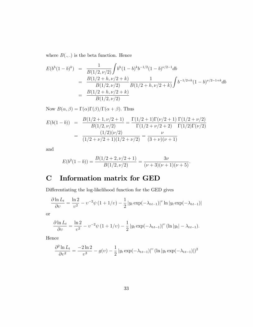
where B(:; :) is the beta function. Hence

E(bh(1� b)k) =1

B(1=2; �=2)

Zbh(1� b)kb�1=2(1� b)�=2�1db

=B(1=2 + h; �=2 + k)

B(1=2; �=2)

1

B(1=2 + h; �=2 + k)

Zb�1=2+h(1� b)�=2�1+kdb

=B(1=2 + h; �=2 + k)

B(1=2; �=2)

Now B(�; �) = �(�)�(�)=�(�+ �): Thus

E(b(1� b)) =B(1=2 + 1; �=2 + 1)

B(1=2; �=2)=�(1=2 + 1)�(�=2 + 1)

�(1=2 + �=2 + 2)

�(1=2 + �=2)

�(1=2)�(�=2)

=(1=2)(�=2)

(1=2 + �=2 + 1)(1=2 + �=2)=

�

(3 + �)(� + 1)

and

E(b2(1� b)) =B(1=2 + 2; �=2 + 1)

B(1=2; �=2)=

3�

(� + 3)(� + 1)(� + 5):

C Information matrix for GED

Di¤erentiating the log-likelihood function for the GED gives

@ lnLt@�

=ln 2

�2� ��2 (1 + 1=�)� 1

2jyt exp(��tpt�1)j� ln jyt exp(��tpt�1)j

or

@ lnLt@�

=ln 2

�2� ��2 (1 + 1=�)� 1

2jyt exp(��tpt�1)j� (ln jytj � �tpt�1):

Hence

@2 lnLt@�2

=�2 ln 2�3

� g(�)� 12jyt exp(��tpt�1)j� (ln jyt exp(��tpt�1)j)2

33

and

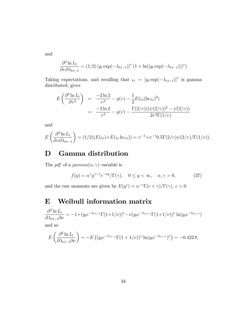
@2 lnLt@�@�tpt�1

= (1=2) jyt exp(��tpt�1)j� (1 + ln(jyt exp(��tpt�1)j)�)

Taking expectations, and recalling that & t = jyt exp(��tpt�1)j� is gammadistributed, gives

E

�@2 lnLt@�2

�=

�2 ln 2�3

� g(�)� 12E(& t(ln & t)

2)

=�2 ln 2�3

� g(�)� �(2=�)(( (2=�))2 � �(2=�))

2�2�(1=�)

and

E

�@2 lnLt@�@�tpt�1

�= (1=2)(E(& t)+E(& t ln & t)) = ��1+��10:5�(2=�) (2=�)=�(1=�)):

D Gamma distribution

The pdf of a gamma(�; ) variable is

f(y) = � y �1e��y=�( ); 0 � y <1; �; > 0; (37)

and the raw moments are given by E(yc) = ��c�(c+ )=�( ); c > 0:

E Weibull information matrix@2 lnLt@�tpt�1@�

= �1+(yte��tpt�1�(1+1=�))���(yte��tpt�1�(1+1=�))� ln(yte��tpt�1)

and so

E

�@2 lnLt@�tpt�1@�

�= �E

�(yte

��tpt�1�(1 + 1=�))� ln(yte��tpt�1)�

�= �0:422 8;

34

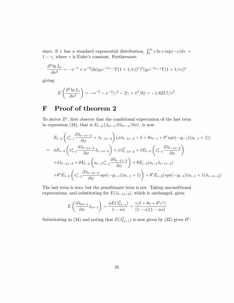
since, if x has a standard exponential distribution,R10x lnx exp(�x)dx =

1� ; where is Euler�s constant. Furthermore

@2 lnLt@�2

= ���2 + ��2(ln(yte��tpt�1�(1 + 1=�))�)2(yte

��tpt�1�(1 + 1=�))�

giving

E

�@2 lnLt@�2

�= ���2 � ��2( 2 � 2 + �2=6) = �1:823 7=�2:

F Proof of theorem 2

To derive B�; �rst observe that the conditional expectation of the last termin expression (34), that is Et�2 (�tpt�1:@�tpt�1=@�) ; is now

Et�2

�x�t�1

@�t�1pt�2@�

+ �t�1pt�2

�(��t�1pt�2 + � + �ut�1 + ��sgn(�yt�1)(ut�1 + 1))

= �Et�2

�x�t�1

@�t�1pt�2@�

�t�1pt�2

�+ ��2t�1pt�2 + �Et�2

�x�t�1

@�t�1pt�2@�

�+��t�1pt�2 + �Et�2

�ut�1x

�t�1

@�t�1pt�2@�

�+ �Et�2(ut�1�t�1pt�2)

+��Et�2

�x�t�1

@�t�1pt�2@�

sgn(�yt�1)(ut�1 + 1)�+ ��Et�2(sgn(�yt�1)(ut�1 + 1)�t�1pt�2)

The last term is zero, but the penultimate term is not. Taking unconditionalexpectations, and substituting for E(�t�1pt�2); which is unchanged, gives

E

�@�tpt�1@�

�tpt�1

�=�E(�2tpt�1)

1� a�+ (� + �c+ ��c�)

(1� a)(1� a�)

Substituting in (34) and noting that E(�2tpt�1) is now given by (32) gives B�:

35

REFERENCES

Andersen, T.G., Bollerslev, T., Christo¤ersen, P.F., and F.X. Diebold (2006).Volatility and correlation forecasting. In: Elliot, G., Granger, C. andA. Timmerman, (Eds.), Handbook of Economic Forecasting, 777-878.Amsterdam: North Holland.

Bollerslev, T. (1986). Generalized autoregressive conditional heteroskedas-ticity. Journal of Econometrics, 31, 307-327.

Creal, D., Koopman, S.J., and A. Lucas (2010). Generalized autoregres-sive score models with applications. Working paper. Earlier versionappeared as: �A general framework for observation driven time-varyingparameter models�, Tinbergen Institute Discussion Paper, TI 2008-108/4, Amsterdam.

Davidson, J. (2000). Econometric Theory. Blackwell: Oxford.

Engle. R.F. (2002). New frontiers for ARCH models. Journal of AppliedEconometrics, 17, 425-46.

Engle, R.F. and J.R. Russell (1998). Autoregressive conditional duration: anew model for irregularly spaced transaction data. Econometrica, 66,1127-1162.

Engle, R.F. and G.M. Gallo (2006). A multiple indicators model for volatil-ity using intra-daily data. Journal of Econometrics, 131, 3-27.

Fiorentini, G., G. Calzolari and I. Panattoni (1996). Analytic derivativesand the computation of GARCH estimates. Journal of Applied Econo-metrics, 11, 399-417.

Gonzalez-Rivera, G., Senyuz, Z. and E. Yoldas (2010). Autocontours: dy-namic speci�cation testing. Journal of Business and Economic Statis-tics, (to appear).

Harvey, A.C. and T. Chakravarty (2009). Beta-t-EGARCH. Working pa-per. Earlier version appeared in 2008 as Cambridge Working paper inEconomics, CWPE 0840.

Linton, O. (2008). ARCH models. In The New Palgrave Dictionary ofEconomics, 2nd Ed.

36

Nelson, D.B. (1990). Stationarity and persistence in the GARCH(1,1)model. Econometric Theory, 6, 318-24.

Nelson, D.B. (1991). Conditional heteroskedasticity in asset returns: a newapproach. Econometrica, 59, 347-370.

Straumann, D. (2005). Estimation in Conditionally Heteroskedastic TimeSeries Models, Lecture Notes in Statistics, 181, Springer, Berlin.

Taylor, J. and A. Verbyla (2004). Joint modelling of location and scaleparameters of the t distribution. Statistical Modelling, 4, 91-112.

Taylor, S. J., (1986). Modelling Financial Time Series. Wiley: Chichester.

Taylor, S. J., (2005). Asset Price Dynamics, Volatility, and Prediction.Princeton University Press: Princeton.

van der Vaart, A.W. (1998). Asymptotic Statistics. Cambridge: CUP.

Varanasi, M.K. and B. Aazhang (1989). Parametric generalized Gaussiandensity estimation. Journal of the Acoustical Society of America, 86,1404-15.

Za¤aroni, P. (2009). Whittle estimation of EGARCH and other exponentialvolatility models. Journal of Econometrics, 151, 190-200.

Zivot, E. (2009). Practical issues in the analysis of univariate GARCHmodels. In Anderson, T.G. et al. Handbook of Financial Time Series,113-155. Berlin: Springer-Verlag.

37