Export Failure and Its Consequences:

Evidence from Colombian Exporters∗

Jesse Mora†

November 26, 2014

Job Market Paper

(Most recent draft HERE )

Abstract

Exporters pay high fixed costs to enter foreign markets, yet the majority will not exportbeyond one year. What happens to these exporters after they fail abroad? For thesefirms, exporting likely resulted in heavy profit losses. Despite this, trade literatureoften views exporting as a harmless exercise based on a simple cost-benefit analysisof foreign profits. This rationale ignores the differential effect export failure may haveon financially-constrained firms. I develop a heterogeneous-firm model with financialconstraints and marketing costs to show how export failure can: 1) make the liquidityconstraint more likely to bind, 2) force financially-constrained firms to limit marketingexpenditure and, hence, decrease domestic sales, and 3) induce some firms to default.Using Colombian firm-level data and three identification techniques (DD, PSM, andIV), I provide empirical support for these propositions. I find evidence that exportfailure has a differential impact on financially-constrained firms. These firms have ahigher probability of going out of business, lower domestic revenue, and lower domesticrevenue growth after exporting; the findings are robust to comparisons with similarsuccessful exporters and even non-exporters.

JEL Classification: F10, F14, F36, G20, G33.Keywords: Export failure, market linkages, financial constraints, heterogeneous firms.

∗I am grateful to Alan Spearot, Nirvikar Singh, Jon Robinson, Jennifer Poole, and Johanna Francis for theirinvaluable guidance and support. I thank Robert Feenstra, Katheryn Russ, Federico Dıez, Costas Arkolakis, TiborBesedes, Peter Morrow, Sven Arndt, JaeBin Ahn, Kenneth Kletzer, Justin Marion, Carlos Dobkin, Grace Gu, GeorgeBulman, Ajay Shenoy, Dario Pozzoli, Manuel Barron, Pia Basurto, Evan Smith and seminar participants at the UCSCMicroeconomics Workshop, UCSC Department Seminar, University of San Francisco, Western Economics AssociationAnnual Conference, and Midwest International Trade Conference for very helpful comments and discussions. Igratefully acknowledge the Department of Economics at University of California, Santa Cruz for financial supportand access to the Colombian customs data.†Correspondence: Department of Economics, University of California, Santa Cruz. Email : jmora4@ucsc.edu

Homepage: jessemora.weebly.com

I Introduction

Exporting allows firms to reach more consumers, potentially earn higher profits, and diversifyagainst risk in the home market. Yet few firms export (Bernard and Jensen, 2004; Brooks, 2006).While several factors affect the costs and benefits of exporting, fixed export costs are particularlyimportant in limiting international trade. These costs are estimated to be around half a millionUS dollars for a single firm in Latin America (Das, Roberts, and Tybout, 2007; Morales, Sheu,and Zahler, 2011), and often exceed export revenue in the first years of exporting.1 In Colombia,for example, foreign revenue in the 1996–2010 period for first-time exporters is about US $200,000on average and US $13,000 for the median firm. Since the majority of firms are unable to exportbeyond one year (Eaton, Eslava, Kugler, and Tybout, 2007), it is likely the exporting resulted inprofit losses for unsuccessful exporters.

What happens to those firms that try to export but fail? The trade literature often viewsexporting as a harmless exercise based on a simple cost-benefit analysis of foreign profits, wherethe most productive firms export and there is no uncertainty in export success. And, from thisperspective, there is no additional cost or benefit to export failure. However, export failure canhave an effect on domestic production: it can be positive if firms learn from exporting, or negativeif export failure has a negative feedback effect. There are economic reasons to believe that for somefirms the negative effect dominates. For example, firms tend to rely more on external financing forexport sales than for domestic sales (Amiti and Weinstein, 2011), so an unsuccessful exporter cannotsimply refocus its resources towards domestic production and ignore foreign losses. Moreover, afirm’s financial constraint might tighten due to the addition of export debt but little or no incomingforeign revenue. The tightened financial constraint may mean fewer financing options for domesticoperations, limiting hiring, marketing, capital investments, and even operating cash flow. Thisdifferential effect on financially-constrained firms means that the negative consequences of exportfailure, not just the probability of export failure, lower expected returns from exporting.

In this paper, I examine the consequences of export failure. I develop a partial-equilibrium modelthat explains how a failed export attempt when accompanied with financial frictions can have anegative feedback on existing domestic operations. The model with heterogeneous firms showsthat there exists a set of exporters for which export failure can have lasting negative consequences,including firm death. In addition, I find empirical support for this model. Using Colombian firm-level data and three identification techniques (difference-in-difference, propensity score matching,and instrumental variable methods), I show that export failure is associated with reduced economicperformance in the domestic market. I find that financially-constrained unsuccessful exporters havea higher probability of default after attempting to export, and those that are able to survive havelower revenue and lower revenue growth. The effect, just as expected from the theoretical model,is robust to comparisons with similar successful exporters and even non-exporters. No paper to myknowledge focuses on failed exporters, provides stylized facts about these firms, nor links export

1Export revenue tends to be small for first time exporters (Rauch and Watson, 2003; Esteve-Perez, Manez-Castillejo, Rochina-Barrachina, and Sanchis-Llopis, 2007).

1

failure with poor domestic market performance. My work fills this gap.

The theoretical model builds the intuition for the empirical analysis. Since I am interestedin the ex post effects of entering a foreign market, I model the firm’s profit-maximization prob-lem after export failure has been determined.2 The model focuses on failed exporters, but alsocompares these firms with successful exporters and non-exporting firms; successful exporters andnon-exporting firms provide counterfactuals for the failed exporters. Exporting has a differentialimpact on domestic operations because of financing needs and the existence of financial frictions.I assume firms borrow twice to pay for upfront costs: the first loan is to pay the export fixed costand the second is to pay for domestic operations (marketing and upfront labor costs). Firms usetheir production-entry expenditure as collateral for the loans; this collateral is an asset necessaryfor production. I follow Manova (2013) in modeling financial frictions and Arkolakis (2010) in mod-eling marketing costs. To these I add an element of uncertainty in export success. Uncertainty isresolved after paying a search fee (the export fixed costs); the search fee gives a firm a chance torandomly match with a foreign distributor. Since a foreign distributor is necessary to sell any quan-tity abroad, export failure results when a firm is unable to find a suitable match. The probabilityof export failure is known and exogenous to the model, therefore similar-productivity firms maydiffer in export success. Furthermore, since export failure results in new debt but no additionalrevenue, it tightens the liquidity constraint and diminishes the maximum amount firms can borrowto pay for domestic operations. In the model, I demonstrate how small and medium-sized firms canbecome financially constrained, decrease domestic sales, or even default because of a failed exportattempt.

In the empirics I test the propositions of the model while also considering alternative explana-tions for the stylized facts. I provide robust evidence that a failed exporting attempt has a negativeimpact on a firm’s domestic market performance. A firm may even pay the ultimate price and goout of business because of its failed export attempt. Specifically, export failure results in lowerdomestic revenue, lower domestic revenue growth, and a higher probability of going out of busi-ness. In the medium run—and in some cases the short run—the association is strong even whencomparing unsuccessful exporters with matched non-exporters and successful exporters.3 Since thedifferences are statistically insignificant in the long run, a firm that manages to keep its doors opencan over come the negative shock. Note, however, that since export failure may lead to firms ex-iting the domestic market, the long-run estimates may suffer from attrition.4 Finally, to addressendogeneity concerns, I follow Hummels, Jørgensen, Munch, and Xiang (2014) and instrument forexport success based on plausibly exogenous market changes at the product level in foreign markets.The instrument contains rich variation across products and destinations, so its impact on a firm

2In the ex-ante export-entry decision, both the cost of export failure the probability of export failure lowerexpected profit from exporting and lead to fewer firms exporting.

3I define the short run as the year firms first export, t = 0; medium run as the following five years, t = 1 to 5;and long run as the remaining “after” periods, t > 5. I explain why I make a distinction between these three periodsin Section IV.

4The levels and Poisson estimates include zero values for firms that exit the domestic market and show thatattrition works against finding any negative long-run effects.

2

varies considerably. Since the instrument is the plausibly exogenous change in the foreign market,firm shocks that affect both the domestic market and the probability of export failure should notinfluence the estimates. The medium-run differences using the IV approach continue to be strongand statistically significant for the three outcome variables.

The work in this paper complements various strands of the literature. It contributes to thefirm heterogeneity literature by providing a better understanding of exporting costs, and thus ofthe firm export-entry decision.5 This paper also contributes to the literature quantifying exportcosts. Das et al. (2007) and Morales et al. (2011) calculate a fixed dollar amount to export fixedcosts, and Smeets, Creusen, Lejour, and Kox (2010) quantify how a home-country’s institutionscan effect export fixed costs. These studies differ from my work in that I focus on the prolongedcosts—measured by the loss of domestic revenue and increased probability of going out of business—associated with export failure. Integrating the costs found in this paper into estimates of fixed costsmay explain why the estimated fixed export costs are so high.

This paper also contributes to the literature on export survival.6 The export survival liter-ature includes studies using bilateral trade-flow data (Nicita, Shirotori, and Klok, 2013; Besedesand Prusa, 2011, 2006a,b) and firm-level data (Stirbat, Record, and Nghardsaysone, 2013; Cadot,Iacovone, Pierola, and Rauch, 2013; Esteve-Perez et al., 2007; Tovar and Martınez, 2011; Albornoz,Calvo Pardo, Corcos, and Ornelas, 2012). The focus of the existing literature is on understandingexport survival, rather than understanding the consequences of export failure. Albornoz et al. (2012)develop a model that explains why firms have low export survival; in their model a firm can onlyinfer its profitability abroad after exporting. In their model, however, there are no consequences toexport failure. Besedes and Prusa (2011) show that differences in export survival at the countrylevel explain differences in long-run export performance. I construct a model and implement anempirical strategy using firm-level data that directly links export failure and firm performance inthe domestic market. Thus, my work identifies a channel through which firm export survival canhave welfare effects at the national level.

More generally, this paper contributes to the literature on financial frictions and internationaltrade. This literature explains how financial frictions affect a firm’s decision to enter a foreignmarket. Manova (2013), Feenstra, Li, and Yu (2013), and Chaney (2013) identify a mechanism bywhich financial frictions can affect trade. Manova (2013) shows how financial frictions can affectboth which firms export and how much they export. Feenstra et al. (2013) find that banks imposemore stringent credit constraints on exporting firms, when compared with non-exporting firms.Antunes, Opromolla, and Russ (2014) examine the riskiness involved in financing exporting firms.They find that exporters, compared with non-exporters, are less likely to go out of business and,conditional on going out of business, more likely to default. The export failure results found in this

5For a sample of the heterogeneous literature see Melitz (2003); Verhoogen (2008); Melitz and Ottaviano (2008);Bernard and Jensen (2004); Bernard, Jensen, Redding, and Schott (2007); Bernard, Redding, and Schott (2011);Helpman, Melitz, and Yeaple (2004).

6A related field is work on firm’s and entrepreneur’s overall success. See Ucbasaran, Shepherd, Lockett, and Lyon(2013) for a summary of the literature.

3

paper may explain another reason exporters are more likely to default.

Finally, this paper adds to the literature on the linkages between the domestic and exportmarkets. Ahn and McQuoid (2013) find that export and domestic revenue are substitutes. Theyfind that capacity-constrained firms lower domestic sales when experiencing a positive export shock.McQuoid and Rubini (2014) differentiate between successful and unsuccessful exporters and findthat “transitory” exporters have a larger drop in sales than “perennial” exporters in the domesticmarket when exporting. They focus on the immediate, short-run opportunity costs of exporting. Iadd to this literature by showing that this linkage does not end when a firm stops exporting; I showthat the effect is prolonged and larger when an unsuccessful exporter is financially constrained. Rhoand Rodrigue (2010) find that exporters have slower domestic revenue growth than non-exportingfirms. They argue that previous models overestimate the sized of fixed export costs. My workdiffers in that I focus on the prolong effects on financially-constrained unsuccessful exporters, whilethey study the linkages for continuous exporters. Lastly, other papers identify trade-offs betweenthe home and foreign market due to a firm’s investment decision (Spearot, 2013), entry and exitdecision (Blum, Claro, and Horstmann, 2013), and pricing decision (Soderbery, 2014).

The rest of the paper is organized as follows. Section II describes the data and provides stylizedfacts about new exporters. Section III introduces a partial-equilibrium model, demonstrating howexport failure can have repercussions in the home market. Section IV implements the identificationstrategy and provides some robustness checks. Section V concludes.

II Stylized Facts for New Exporters and Data Description

In this section, I describe the data, provide summary statistics, and offer empirical motivation formy findings. I use an event study analysis to compare the domestic market performance—beforeand after entering a foreign market—of firms exporting at the same time, but differing in exportsuccess. The analysis identifies stylized facts about the two types of new exporters (successful andunsuccessful) and presents a more complete picture of the association between domestic marketperformance and exporting. See Table 1 for a summary of the stylized facts.

Table 1: Summary of Three Stylized Facts

Fact 1: Unsuccessful exporters are more likely to exit the domestic market after exportingthan their successful counterparts, and financially constrained unsuccessful exportershave the highest exit rates.

Fact 2: Unsuccessful exporters decrease domestic revenue after exporting, and financiallyconstrained unsuccessful exporters decrease revenue the most.

Fact 3: All financially constrained exporters, irrespective of their success abroad, have lowerdomestic revenue growth after exporting.

4

II.1 Data sources and sample

I use Colombian firm level data to analyze the link between export failure and domestic marketperformance. Using Colombian data for this analysis is ideal for several reasons. First, I am ableto merge domestic financial data with trade data. The trade data help determine whether or notfirms are successful at exporting, the products firms export, and the destination of these products.The financial data provide information on domestic revenue, and also on various other financialvariables (eg. assets, liabilities, etc.). While the two data sets have been used before, to myknowledge I am the first to use both together. Second, since firms in developing countries have ahigher probability of export failure than those in developed ones (see Besedes and Prusa 2011), theconsequence associated with such failure may be more acute in developing countries; thus it makessense to use data from a developing country, such as Colombia, in the analysis. Finally, these dataprovide a fairly long panel (16 years) and, for many firms, we can observe firm behavior severalyears before and after first exporting.

I use Colombian customs data as reported by the Colombian National Directorate of Taxes andCustoms (DIAN) to get firm-level exports for the 1994–2011 period. Each transaction includes afirm tax identifier (which is time-invariant), a product code, trading partner, and the free-on-board(FOB) export value in US dollars and Colombian pesos.7 Although the data are at the transactionlevel, I aggregate to the annual level. I do this for two reasons. First, exporting is intrinsicallydiscrete; thus, it makes more sense to aggregate. Aggregating eliminates seasonal fluctuation andaccounts for the fact that some firms import infrequently to take advantage of economies of scaleand to account for delivery lags (Alessandria, Kaboski, and Midrigan, 2010). Second, I aggregatethe trade data to match the level of aggregation for the financial data.

I use Colombian financial data as reported by the Superintendency of Corporations (“Superin-tendencia de Sociedades”) to get balance sheet information for firms producing in the 1995–2011period. These data include only firms that fall under the jurisdiction of the agency, which is partof the Colombian Ministry of Commerce, Industry and Tourism; they are publicly available in the“Sistema de Informacion y Reporte Empresarial” (SIREM) database. The financial data are self-reported and must be provided annually by law. These data do not include the universe of firms anddo not come from a survey, but do include most of the value added in the real economy. Accordingto SIREM, the data account for 95% of the GDP in the real economy and cover on average of 25,000firms per year (see SIREM User Guide). They include firms in the following categories: privatelimited companies, public limited companies, joint ventures, simple limited partnerships, limitedjoint-stock partnerships, foreign companies, and self-employed businesses.8 The financial data in-clude the firm name, sector, tax identifier, year, and various balance sheet information (liabilities,assets, revenue, etc.) in Colombian pesos. There is a possibility that a firm did not report databecause it did not have to (firms that are in the process of shutting down do not have to reporttheir financial information) or because the firm chose to break the law. In either case, if a firm does

7I ignore firms whose tax identifiers do not conform to the standard nine-digit number. The trade data are thesame used in Eaton et al. (2007) and add up to within one percent of UN COMTRADE exports.

8See Table A.1 for a complete list of included and excluded firm types.

5

not report its financial data, I interpret this as representing a bad outcome and simply treat thefirm as exiting the domestic market.

I merge the two data sets using the year and tax identifier and make additional restrictionsto get the data sample used in this paper. I classify firms as unsuccessful exporters based on thetrade data; if a firm is unable to export for more than one year, I consider such a firm as a failedexporter. However, I allow successful exporters to exit and enter the export market. I exclude afirm if it has missing financial data in any period between its first and last year of production; Ido this because there are very few such firms and keeping them would result in missing data forreasons other than the firm exiting the domestic market. I make the additional requirement thatall firms have financial data for at least three consecutive years: two years before exporting and theyear of exporting. Thus, in my sample, at a minimum, all firms have one domestic revenue growthobservation before exporting and one observation after. Finally, since new exporters are the focusof this paper, I exclude continuous exporters and non-exporters for most of the estimates. I definecontinuous exporters as firms that have trade data in 1994, the first year available with trade data,and non-exporters as firms with no export data in the periods analyzed. The 2010 export cohort isexcluded since, for these firms, there is not enough information in the after period to calculate themedium-rum effect for the firm exit variable; keeping this group in the sample does not alter theresults. I end up with 15,381 firm-year observations, 838 successful exporters, and 574 unsuccessfulexporters.9

Variable definitions

There are three main outcome variables: Domestic Revenue, Domestic Revenue Growth, and Exitfrom the domestic market. Since the financial data only include total revenue by firm, I subtracttotal exports from total revenue to calculate domestic revenue.10 Domestic Revenue equals eitherthe level domestic revenue in Colombian Pesos or the natural log of domestic revenue for firm i attime t. Domestic Revenue Growth for firm i at time t equals the difference in log domestic revenuebetween time t and time t − 1. Exits from the domestic market equals one if the firm exits thedomestic market, and zero otherwise. Note that this last variable does not vary by time since firmsin the sample enter and exit only once; so estimates for the probability of exiting from the domesticmarket do not come from panel regressions and do not include firm fixed effects.

The main covariates of interest are the following: successful exporter (Sit), unsuccessful exporter(Uit), and a measurement of financial constraint (NFV ). Uit equals one for new exporters that failto export beyond a 12-month period, and zero otherwise. Thus, a firm that exports in two calendaryears can still be classified as unsuccessful. Sit equals one for all other new exporters, and zerootherwise. Since I am interested in comparing financially constrained firms, I separate financially-and non-financially-constrained firms. A firm is financially vulnerable (NFV = 0) if the ratio of

9I include as many non-exporters as unsuccessful exporters in the Propensity Score Matching estimates.10This might introduce measurement error in the Domestic Revenue variable if firm financial data do not match

the timing of the trade data.

6

cash flow from operations to total assets is less than the median at the time of first exporting(t = 0), and a firm is financially vulnerable (NFV = 1) if the same ratio for a firm is above or equalto the median. This ratio measures how well a company is able to generate cash from its assets.A smaller ratio implies that the firm will have less cash available for future expenditures, and thuswill be more in need of external financing. This measurement is widely use in the literature (Ahnand McQuoid, 2013; Whited and Wu, 2006; Kaplan and Zingales, 1997). As a robustness check, Iuse the median total asset as a measurement for the financial constraint.

II.2 Summary statistics

The trade data show why focusing on unsuccessful exporters is important.11 The importance ofthese firms, however, may be overlooked in the overall sample. For instance, I find that on averageabout nine thousand Colombian firms export in any given year. Of these, 2,458 are continuousexporters, 4,242 are successful exporters, and 1,817 are unsuccessful exporters (see Appendix TableA.2). On average, continuous exporters account for most of the export value (almost three fourthsof all exports), successful exporters account for a bit over one fourth, and unsuccessful exportersaccount for the rest (less than one percent). Yet unsuccessful exporters make up the vast majorityof new exporting firms; on average, unsuccessful exporters account for almost two thirds of newexporters, and successful exporters account for the rest. While unsuccessful exporters tend to exportless than their share of firms, they still represent about a third of the export value coming fromnew exporters.

The financial data put the importance of exporters in context. On average, the financial datacover over fifteen thousand firms per year; 12 percent are continuous exporters, 70 percent arenon-exporters, 12 percent are successful exporters, and 5 percent are unsuccessful exporters. WhileI find that 30 percent of firms export at least once, the number is inflated by the fact that thedata do not come from a random sample, and the firms in the sample tend to be fairly large. Infact, non-exporters on average have total sales equal to about 5 billion Colombian pesos (about US$2.5 million), continuous exporters average about 50 billion, successful exporters average about 27billion, and unsuccessful average about 15 billion. Of this value, continuous exporters receive 23percent from exporting, successful exporters receive 14 percent, and unsuccessful exporters receiveless than 1 percent. These data confirm findings in other papers: few firms export, only the mostproductive firms export, those that do export start small.

11See Eaton et al. (2007) for a through discussion on the export dynamics of Colombian firms. Note, however,that I do not use the same definitions used in that paper, and so the numbers in this paper will not match those ofEaton et al. (2007). For example, I define unsuccessful exporters, what they call “single year” exporters, as firmsthat are unable to export for more than 12 months and they define them as firms that exported in year t but not int− 1 or t+ 1.

7

II.3 Empirical motivation

I find that domestic market performance is correlated with exporting, and the association dependson both the export success and financial vulnerability of a firm; that is, the effect depends on whetheror not the firm was successful at exporting and on whether or not the firm was financially vulnerablewhen it first exported. Looking at three outcome variable (firm exits from domestic production,domestic revenue, and domestic revenue growth), I identify three stylized facts regarding exportfailure and domestic market performance.

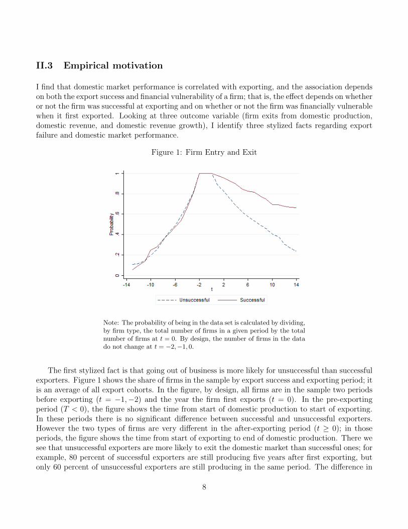
Figure 1: Firm Entry and Exit

Note: The probability of being in the data set is calculated by dividing,by firm type, the total number of firms in a given period by the totalnumber of firms at t = 0. By design, the number of firms in the datado not change at t = −2,−1, 0.

The first stylized fact is that going out of business is more likely for unsuccessful than successfulexporters. Figure 1 shows the share of firms in the sample by export success and exporting period; itis an average of all export cohorts. In the figure, by design, all firms are in the sample two periodsbefore exporting (t = −1,−2) and the year the firm first exports (t = 0). In the pre-exportingperiod (T < 0), the figure shows the time from start of domestic production to start of exporting.In these periods there is no significant difference between successful and unsuccessful exporters.However the two types of firms are very different in the after-exporting period (t ≥ 0); in thoseperiods, the figure shows the time from start of exporting to end of domestic production. There wesee that unsuccessful exporters are more likely to exit the domestic market than successful ones; forexample, 80 percent of successful exporters are still producing five years after first exporting, butonly 60 percent of unsuccessful exporters are still producing in the same period. The difference in

8

Figure 2: Ln(Domestic Revenue): Unsuccessful Exporters(Financially-Constrained Firms)

Note: The estimates control for firm fixed effects and year fixed effects.The omitted group is financially-constrained, unsuccessful exporters attime t = −1.

survival rates is increasing over time. However, this difference disappear in the long run if I comparethe probability of exiting the domestic market conditional on producing at time t (the hazard rate).I get similar results if I separate financially vulnerable firm from the two types of exporters; thedifference is that financially vulnerable firms are more likely to exit the domestic market than theirtheir non-financially vulnerable counterparts.

The second stylized fact is that after export failure domestic revenue decreases for unsuccessfulexporters and the drop is more pronounced for financially vulnerable ones. In event-study Figure2, we can see how such financially vulnerable unsuccessful exporters acted in all periods beforeand after exporting relative to t = −1 (the year before exporting).12 The figure comes from aregression with firm and year fixed effects that includes my whole data sample. In the before-exporting period, domestic revenue grows as firms gets closer to exporting, but the trend changessignificantly afterward. In the before-exporting periods these firms were in an upward trajectory; so,for these firms, exporting was not a last resort effort to stay in business. Domestic revenue decreasesfor these unsuccessful exporter in the after-exporting period and eventually stalls at pre-exportinglevels. The drop is quite significant in the short term; relative to t = −1, domestic revenue decreasesabout 10 percent the year the firm exports (t = 0) and this decreases to about 25 percent the nextfive years. For the median firm in t = −1, whose total revenue is about 4 billion pesos (roughlyUS$ 2 million), this would account for a drop of 400 million pesos the year the firm first exports

12For similar figures using matched data see Figures A.1, A.2, and A.3 in the Appendix.

9

and 1 billion pesos each of the following five years.

Figure 3: Ln(Domestic Revenue): Unsuccessful vs. Successful Exporters(Financially-Constrained Firms)

Note: Regression includes firm fixed effects and year fixed effects.

There may be numerous explanations why financially vulnerable unsuccessful exporters see adrop in domestic revenue after exporting. One possible explanation is that the figure may becapturing firm trends, so a difference-in-difference framework is more appropriate than a pre- andpost-exporting analysis. A difference-in-difference framework may be necessary if, for example,firms tend to export at peak production, and a decrease in domestic revenue after the peak may beexpected. In event study Figure 3 I estimate the difference between financially vulnerable successfulexporters and unsuccessful ones; the figure comes from the same regression as Figure 2. There aretwo benefits to using an event study analysis for this comparison. First, we can see if the “control”group (successful exporters) has a similar trend to the “treatment” group (unsuccessful exporters)in the before-exporting periods. We see in the figure that there are no statistically significantdifferences in the pre-exporting periods; so both financially vulnerable successful and unsuccessfulexporters have similar trends in domestic revenue before exporting. The second benefit of theevent study analysis is that we can see how both firm types react in the domestic market afterexporting relative to t = −1. The differences in these periods are stark. Financially vulnerable,successful exporters are much better off compare to those that are unsuccessful; these differencesare statistically significant. The difference is such that domestic revenue for financially vulnerablesuccessful exporters does not decrease at t = 0 or any other post-exporting periods, relative tot = −1.

To check if firm-specific trends are driving my results, I replicate the figures above using domestic

10

revenue growth as the outcome variable.13 These results identify a third stylized fact: domestic rev-enue decreases after exporting for both financially vulnerable unsuccessful and successful exportersin the short and medium run. In event study Figure 4, we again see how financially vulnerableunsuccessful exporters acted before and after exporting relative to t = −1 (the year before ex-porting).14 While domestic revenue growth picks up before a firm exports, this growth is, for themost part, not statistically different than that of the t = −1 period. In the after-exporting period,however, there is a large and statistically significant drop in the growth rate. Domestic growthdecreases by about 20 percent the year the firm first exports, and while growth improves after that,it is still lower than the t = −1 growth for several years. Growth eventually returns to its trendabout five years after exporting.

Figure 4: ∆Ln(Dom. Revenue) for Unsuccessful Exporters(Financially-Constrained Firms)

Note: Regression includes firm fixed effects and year fixed effects. Theomitted group is constrained, unsuccessful exporters at time t = −1.

I compare the difference in domestic revenue growth between financially vulnerable successfuland unsuccessful exporters to see how their trends differ. While these successful exporters are doingrelatively worse in the before-exporting period, these differences are not statistically significant.When comparing these firms in the after-exporting period, we see a relative increase for successfulexporters, but the difference is again not statistically significant (see event study Figure 5). Partof the reason I may not find a statistically significant difference may be that liquidity constraints

13Since the regression includes firm fixed effects, using this outcome variable removes time-invariant, firm-specificgrowth trends.

14For similar figures using matched data see Figures A.4, A.5, and A.6 in the Appendix.

11

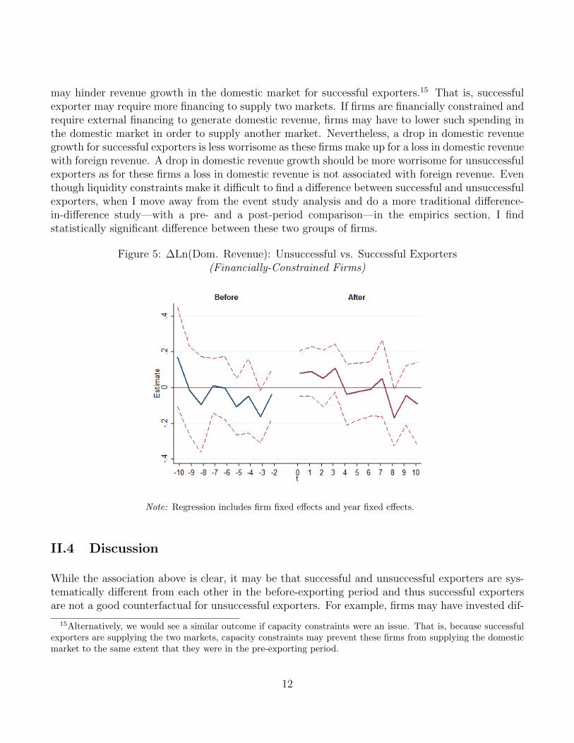
may hinder revenue growth in the domestic market for successful exporters.15 That is, successfulexporter may require more financing to supply two markets. If firms are financially constrained andrequire external financing to generate domestic revenue, firms may have to lower such spending inthe domestic market in order to supply another market. Nevertheless, a drop in domestic revenuegrowth for successful exporters is less worrisome as these firms make up for a loss in domestic revenuewith foreign revenue. A drop in domestic revenue growth should be more worrisome for unsuccessfulexporters as for these firms a loss in domestic revenue is not associated with foreign revenue. Eventhough liquidity constraints make it difficult to find a difference between successful and unsuccessfulexporters, when I move away from the event study analysis and do a more traditional difference-in-difference study—with a pre- and a post-period comparison—in the empirics section, I findstatistically significant difference between these two groups of firms.

Figure 5: ∆Ln(Dom. Revenue): Unsuccessful vs. Successful Exporters(Financially-Constrained Firms)

Note: Regression includes firm fixed effects and year fixed effects.

II.4 Discussion

While the association above is clear, it may be that successful and unsuccessful exporters are sys-tematically different from each other in the before-exporting period and thus successful exportersare not a good counterfactual for unsuccessful exporters. For example, firms may have invested dif-

15Alternatively, we would see a similar outcome if capacity constraints were an issue. That is, because successfulexporters are supplying the two markets, capacity constraints may prevent these firms from supplying the domesticmarket to the same extent that they were in the pre-exporting period.

12

ferently or had different debt levels; observable variables that may be different include short-termdebt, long-term debt, short-term labor expenditure, long-term labor expenditure, short-term invest-ment, long-term investment, inventory, property, intangibles (patents, etc.). As seen in AppendixTable A.3, however, most of the differences are not statistically significant. The only exception islong-term investment, successful exporters have over 70 percent more long-term investment thando unsuccessful ones. This applies to both the whole before-exporting period and also just the yearbefore exporting. Successful exporters may have invested and upgraded to become competitiveabroad. These pre-export, observable differences–even if there are few—make it clear that I mustbe careful when making the comparison between successful and unsuccessful exporters. The com-parison is complicated by the fact that there might be unobserved, time-varying differences betweenthe two groups. It may also be that it takes time to reorient the firm to serve only the domes-tic market; that firms experience different negative, long-lasting productivity shocks that correlatewith exporting; or that the two groups export for different reasons and have different trends in theafter exporting period. In the sections below, I attempt to rule out as many of these alternativeexplanations as possible and establish export failure as at least partially responsible for the negativeperformance seen after export failure.

III A Model with Export Failure, Marketing Costs, and

Financial Frictions

In the previous section, I identified four stylized facts about unsuccessful exporters (see Table 1for a summary). In this section, I develop a simple two-country, Melitz-type model with domesticoutcomes as a function of export success that can replicate the stylized facts. I follow Manova (2013)in structuring financial frictions and Arkolakis (2010) in implementing marketing costs. In themodel, firms fail abroad if they are unable to find a suitable match; thus, similar-productivity firmscan differ in export success. Unlike most firm heterogeneity models, which focus on the firm export-entry decision, I focus on the firm’s decision after export success has been determined. I contrast theex post profit-maximizing decisions between non-exporters, unsuccessful exporters, and successfulexporters. I identify three testable predictions from the model: exporting for unsuccessful exporters,compared to successful exporters and non-exporters, results in a tighten financial constraint, lowerdomestic revenue, and a higher probability of default.

III.1 Consumers

Consumers have constant elasticity of substitution (CES) preferences across varieties in each country(h and f). Utility for consumers is specified according to the following form:

U =

(∫iεΩ

cρi di

) 1ρ

13

Here, Ω is the mass of available goods and ci is the consumption of variety i in each country.16

Goods are substitutes, which implies that 0 < ρ < 1 and that the elasticity of substitution between

two goods is given by σ = 11−ρ > 1. Aggregate prices are given by P =

(∫iεΩp

(1−σ)i di

) 11−σ

and

aggregate consumption/aggregate utility per individual is given by U = C =(∫

iεΩcρi di

) 1ρ . Total

revenue and expenditure per individual is given by P ·C = Y . Individuals maximize utility subjectto a revenue constraint:

∫iεΩpicidi = Y . Optimal consumption in each country, per individual who

buys variety i, is given by ci =p−σiP 1−σY . Finally, total consumption of variety i in each country is

given by qi = Lici = Lip−σiP 1−σY , where Li is the number of individuals in a given country who buy

variety i. Li is endogenously determined by a firm’s marketing expenditure.

III.2 Firms

Setup of the model

Firms enter under uncertainty. Firm pay a fixed entry fee, fe, to enter the home market. This feeis in terms of labor and is a tangible asset that can be used as collateral. After paying fe, the firmthen draws a unit labor requirement coefficient, φi, from a known distribution G(φi). All firms mustalso pay an additional overhead labor cost, fd, in order to produce in the home market (similar toMelitz, 2003); this cost is also in terms of labor and wages are normalized to one. Upon receiving itsproductivity draw, the firm decides whether or not to produce; low productivity firms never remainin the market.

After entry, firms must decide whether or not to enter the export market. If the firm decidesto enter the export market, it must pay an export entry fee, fx, which is in terms of labor. Firmsenter the export market under uncertainty and pay this fee to find if they match with a foreigndistributor/partner; a foreign distributor is necessary to sell any quantity abroad. The probabilitythat a firm is successfully matched with a foreign distributor is γ and the probability that it isunable to find a suitable match abroad is (1 − γ). I assume firms are risk-neutral and that γ isdetermined outside of the model.17 For convenience, I assume that unsuccessful exporters do notget any revenue from exporting; I do this as unsuccessful exporters receive a negligible amount ofrevenue from abroad (see Section II.2). For the conclusions to hold, unsuccessful exporters mustlose profits from exporting; that is, the revenue from exporting does not cover the export entry fee,marketing expenditure, and variable cost spent to supply the foreign market. As mentioned in theintroduction, this is likely to be the case for most new exporters.

Firms borrow twice before profits are realized. The first time is to pay exporting fixed costs, fx.

16Since each firm produces only one product, i indexes for both the product and the firm. For convenience, I leaveout country subscripts where the distinction is clear.

17Studies have found that firms upgrade before exporting, increasing export survival (see Bustos, 2011). Butupgrading tends to takes place on the upper end of the distribution and not by financially-constrained firms.

14

The second is to pay for marketing, F (Li), and overhead labor costs in the domestic market, fd. Asin Manova (2013), I assume that firms cannot use profits from a previous period or other savingsto pay for these costs. I also assume that all firms must borrow the full amount of these costs.18 Ifa firm cannot borrow to pay the marketing expenses and overhead labor costs, it loses its collateraland is unable to produce.19 These firms must replace their collateral if they wish to produce in thefuture.

Marketing costs, F (Li), are endogenous and determine the number of individuals a firm reaches.I assume marketing has increasing marginal costs and that firms only use domestic labor in mar-keting for any market. These costs determine how much a firm needs to borrow for marketing.

After borrowing, firms produce and earn profits. Firms use these profits to pay off their debt.See Table 2 for a summary of the sequence.

Table 2: Summary of Sequence of Events

1. Pay entry fee, fe, get productivity draw, and decide whether or not to stay in thedomestic market.

2. Borrow, if exporting is desirable, to pay the export entry fee, fx; this is a matchingfee that allows firms to match with a foreign partner/distributor.

3. Borrow for marketing costs, F (Li), and overhead labor costs, fd.

4. Profits are realized and debt is paid off.

Firm maximization problem before export success has been determined

After the initial productivity draw, there is still uncertainty in the loan repayment for all firms thatborrow and uncertainty in a firm’s matching success for those firms that decide to export. Theprobability that a firm is successfully matched with a foreign distributor is γ and the probabilityof default is λ. Firms only pay the export entry fee if they are, conditional on surviving abroad,better off. All firms with expected foreign profits greater than or equal to zero enter the exportmarket. If the probability of export survival were certain and if there were no financial frictions, themodel would solve to something similar to that in Melitz (2003). The key difference between thismodel and the existing literature is that firms pay fx to find an export match, and as mentioned

18I do this for convenience; for the conclusions of the model to hold, firms need to pay a percentage of the fixedcosts and upfront marketing costs with outside capital. Thus, the conclusions here are more applicable to firms thatare more dependent on outside capital.

19Risk-neutral creditors lend the export entry fee to some firms that, conditional on the firm discovering that it isan unsuccessful exporter, will be unable to borrow the second installment. Creditors charge higher repayment feeswhen repayment is not certain to ensure they do not lose money.

15

above the match success is uncertain.20 By making the export matching probability exogenous, Iabstract from the export-entry decision and instead focus on the decision after export success hasbeen determined. Since matching success is determined outside of the model, and all firms attemptto enter the export market if expected foreign profits are greater than or equal to zero, similar firmscan enter the export market and differ in export success.21

Firm maximization problem after export success has been determined

After export success is determined, there are three types of firms in the market: non-exporters,unsuccessful exporters, and successful exporters. Non-exporters only supply the home market andborrow to pay for the overhead costs, fd, and marketing expenditure, F (Li). Unsuccessful exportersalso only supply the home market, but have additional debt burden because of the export loan.Successful exporters also pay back the export loan, but, unlike unsuccessful exporters, have revenuefrom two or more markets to pay off this debt.22 In this section, I focus on the unsuccessful exporterdecisions and also provide the solutions for the non-exporter and successful exporter decisions.

For unsuccessful exporter i, the ex post maximization problem is as follows:

Eπ(φi) = maxpi,qi,Li

piqi −

qiφi− λBi − (1− λ)fe

(1)

Subject to

qi = Lip−σiP 1−σY (2)

F (Li) = Lβi (3)

piqi −qiφi≥ Bi (4)

λBi + (1− λ)fe ≥ fx + fd + F (Li) (5)

Equation (1) is the profit function. Equation (2) is the total demand for the variety produce by firmi. With CES utility, this is the demand function for individual varieties (see the consumer decisionproblem for details). Equation (3) is the marketing expenditure for the variety produced by firm i.

20This idea is similar to that of Albornoz et al. (2012), but the focus of the model is on the ex post profitmaximization problem, not the ex ante maximization problem.

21The probability of default, as in Manova (2013), is exogenous to the model. Endogenous default would reinforcethe findings of this model. The reason is that firms with a higher probability of default are either not able to borrowor have higher repayment costs. If costs are higher, then the firms that find that exporting is not viable are likelyto become even more constrained and have a higher probability of becoming insolvent than in the exogenous defaultcase. Thus, borrowing becomes even more difficult.

22Expected profits equal the sum of net revenue from the home and, if relevant, foreign markets minus expectedloan repayment. The expected loan repayment is the loan, Bi, times the probability of paying back the loan, λ, plusthe collateral, fe, times the probability of losing the collateral, 1− λ.

16

F (Li) is the amount of labor required to reach Li consumers, and firms must borrow this amount.I assume β > 1 to allow for increasing marginal costs to reaching consumers.

Equation (4) is the firm’s liquidity constraint. Net revenues, excluding the loan, must be largerthan or equal to the loan repayment, Bi. When repaying the loan, firms can at most offer theirnet revenues to the creditor. This constraint is only binding for low productivity firms. Equation(5) is the risk-neutral, creditors’ constraint. Creditors only fund a firm if net returns from the loanare greater than their outside options; this option is normalized to zero. This constraint ensurescreditors do not lose money and thus are always be willing to lend when expected repayment is non-negative. Assuming perfect competition in the credit markets, this constraint holds with equality.fx is the export entry fee and the size of the exporting loan; notice that the firm pays fx, buthas no new revenue. fd is the overhead labor fixed costs in the home market and the size of thedomestic-production loan. F (Li) is the marketing expenditure and the size of the marketing loan.These last three costs are financed using outside capital; although I assume that firms borrow thewhole amount, the conclusions hold as long as firms have to borrow a share of those costs. Bi is therepayment creditors receive when firms repay all of their debt and fe, the entry fee, is the collateralcreditors receive when firms default on their debt.

In the following analysis, I make two key assumptions:

Assumption 1: maxfe−fdfe

, 1β

< λ

Assumption 2: fx > fd

Assumption (1) ensures that fd > (1−λ)fe and βλ > 1. The expected cost of defaulting, (1−λ)fe,cannot be larger than the expected cost of repaying the overhead costs. Otherwise, the expectedcost of borrowing would be higher than the actual cost. It would also mean borrowing costs wouldbe prohibitively high and few firms, if any, would want or be able to borrow. Assumption (2) impliesthat that the fixed costs are higher in the foreign market than in the domestic market; this ensuresthat only the most productive firms export. The necessity of the two assumptions becomes obviousin the following subsections.

III.3 Credit-constrained firm threshold

Maximization problem for unconstrained firms

For financially unconstrained firms, Equation (4) will not bind and these firms will be able to borrowas much as they desire. Substituting Equations (2), (3), and (5) into the maximization problemgives the problem for unconstrained, unsuccessful exporters:

maxpi,Li

Eπi(φi) = Lip1−σi

P 1−σY −Li

p−σiP 1−σY

φi− fx − fd − Lβi

17

Firms set their price by maximizing profits with respect to pi. The profit-maximizing price is thefollowing:

p∗i =σ

σ − 1

1

φi=

µ

φi(6)

Where µ = σσ−1

is the firm’s constant markup above marginal cost. The number of consumers a firm

reaches, Li, increases net revenue, piqi − qiφi

, but also increases marginal marketing costs, βLβ−1i .

By maximizing profits with respect to Li and substituting in the profit-maximizing price, Equation(6), we get the profit-maximizing marketing expenditure:

L∗i =

(Y

σβ

) 1β−1(

µ

Pφi

) 1−σβ−1

(7)

These firms set the marginal cost of marketing equal to the marginal revenue of marketing. Sinceneither the fixed-exporting costs nor foreign revenues affect this decision, all unconstrained firmsin the domestic market, regardless of their classification (non-exporter, unsuccessful exporter, andsuccessful exporter), choose L∗

i . Firms set different L∗i because of differences in productivity, φi.

Furthermore, L∗i is increasing in productivity,

∂L∗i

φi> 0.

Unconstrained firm threshold

For a financially-constrained firm, Equation (4) binds when setting the price and marketing levelsequal to the profit-maximizing p∗i and L∗

i . Intuitively, all firms need to borrow to pay the sameexport entry fee, fx, and have the same collateral, fe, but less productive firms, firms below φC ,earn lower revenues and thus have lower repayment capabilities. For the firm at the constrained-unconstrained threshold, Equation (4) binds and yet the firm still chooses the loan amount it desires.To find this firm, substitute all of the constraints, the profit-maximizing p∗i and L∗

i , and solve forφi. For unsuccessful exporters, this threshold firm, φfailC , is the following:

φfailC =µ

P

(Y

σβ

) 1(1−σ)

(fx + fd − (1− λ)fe

λβ − 1

) 1−ββ(1−σ)

(8)

Had these firms not paid the export entry fee, they would not have the export loan, and would bein better financial health. To find the unconstrained threshold firm had these firms not exported,we set fx = 0. We get the following threshold firm, φdomC , as the before-exporting period thresholdfor all firms before entering the export market or for all non-exporting firms:

φdomC =µ

P

(Y

σβ

) 1(1−σ)

(fd − (1− λ)fe

λβ − 1

) 1−ββ(1−σ)

(9)

Successful exporters have to pay the fixed export costs, just like the unsuccessful exporters, buthave two revenue sources. While all successful exporters sell abroad, only those with productivity

18

above φC export at p∗i and L∗i . The unconstrained threshold firm depends on the size of the foreign

market, foreign prices, and the other trade costs. If the successful exporter enters a foreign marketsimilar to that of the home market, Yh = Yf = Y , with a price level equal to that of the domestictimes the iceberg trade costs, Pf = Ph · τif , then the threshold firm for successful exporters, φsuccC ,becomes:

φsuccC =µ

P

(y

σβ

) 1(1−σ)

(fx + fd − (1− λ)fe

2(λβ − 1)

) 1−ββ(1−σ)

(10)

For a general case, see Appendix A.1.a.23

Proposition 1: Some successful and unsuccessful exporters become liquidity constrained as a resultof exporting. Controlling for firm productivity, unsuccessful exporters are more likely to becomeliquidity constrained than successful exporters (φsuccC < φfailC ).

Proof: The constrained-unconstrained threshold firm for non-exporters is the before exportingthreshold, irrespective of export success. To prove the first part of the proposition, I compare,individually, successful and unsuccessful exporters with non-exporters. To prove the second part Icompare the threshold firm for successful and unsuccessful exporters. See proof in Appendix A.2.

III.4 Credit-constrained firm marketing decision

For liquidity-constrained firms, firms with productivity below φC , choosing the profit-maximizingpi and Li results in Equation (4) binding. These firms are unable to get their desired financingand reduce their need for financing by lowering the number of consumers they reach. This hap-pens because reaching more consumers, higher Li, requires more financing, ∂F (LI)

∂Li= βLβ−1

i , which

increases the repayment necessary to meet creditors’ demands, ∂Bi∂Li

=βLβ−1

i

λ. These two equations

only equal when creditors are guaranteed repayment (λ = 1). An unconstrained, risk-neutral firmdiscounts the repayment by λ. A financially-constrained firm is unable to do discount because ofthe liquidity constraint and sets Li below that of Equation (7). Since this deviation from optimumLi lowers profits, the firm deviates as little as possible to ensure that the creditors break even. Thesecond-best Li for unsuccessful exporters is determined by setting Equation (4) to equality andsubstituting in Equations (2), (3), (5) and (6):

LiY

σ

(µ

Pφi

)1−σ

− Lβiλ

=fx + fd − (1− λ)fe

λ(11)

23An alternative way of thinking about this is by focusing on foreign profits, inclusive of loan repayment costs.Whether or not the threshold loosens or tightens depends on whether foreign profits, inclusive of loan repayment,are positive. Risk-neutral firms enter the export market as long as foreign profits, excluding the loan markup, arepositive. Thus, it is possible that net foreign profits, inclusive of loan repayment costs, are negative.

19

For the before-exporting decision, set fx = 0. This is also the Li chosen by non-exporters. Thus,non-exporters choose Li based on the following equation:

LiY

σ

(µ

Pφi

)1−σ

− Lβiλ

=fd − (1− λ)fe

λ(12)

For financially-constrained successful exporters, the firm’s choice of Li depends on the foreignmarket and the trade costs. So, a previously financially-constrained firm can become more con-strained, less constrained or, even, unconstrained. It depends on the net revenue from the foreignmarket. If the firm enters a similar size market (Yh = Yf = Y ) with a foreign price level equal tothat of the domestic price times the iceberg trade costs (Pf = Ph · τif ), then the successful exporterchooses the following Li in the domestic market:

LiY

σ

(µ

Pφi

)1−σ

− Lβiλ

=fx + fd − (1− λ)fe

2λ(13)

See Appendix A.1.b for a general case.

In all cases above, Li is increasing in productivity, ∂Liφi

> 0 (see Appendix A.3).

Lower threshold for Li

Li is between the profit-maximizing Li (see Equation 7) and the Li that maximizes the left-handside of Equations (11) to (13). Notice that maximizing the left-hand side of the equations withrespect to Li is just like maximizing expected profits with respect to Li, except that the marketing

costs are divided by λ.Lβiλ

is the repayment for the marketing costs, while Lβi is the marketingexpenditure.24 Since 0 < λ < 1, more weight is given to the marketing costs here than in themaximization problem for financially-unconstrained firms. There is no incentive to lower Li beyondthe value that maximizes the left-hand side of the above equation because beyond that point themarginal repayment cost of marketing, βLβ−1

i is lower than the marginal revenue of marketing,piqi − qi

φi; the firm would be better off increasing Li. The Li maximizing the left-hand side of

equations (11) to (13) is given by the following equations:

LCi = λ1

β−1

(Y

σβ

) 1β−1(

µ

Pφi

) 1−σβ−1

(14)

From Equations (7) and (14), we can see that LCi = λ1

β−1L∗i . Since λ < 1 and β > 1, then λ

1β−1 < 1

and LCi < L∗i . Thus, financially-constrained firms always choose an Li that lies between these two

values.

24Lβi is also the expected repayment for the marketing expenditure.

20

Revenues before and after exporting

Domestic revenue (vi) with profit-maximizing price for all firms is piqi = LiY(

µPφi

)1−σ. Li depends

on a firm’s productivity draw and on whether or not the firm is financially constrained. For un-constrained firms, substitute in the profit-maximizing Li (Equation 7) into the domestic revenueEquation to get the profit-maximizing domestic revenue:

v∗i = Yββ−1

(1

σβ

) 1β−1(

µ

Pφi

)β(1−σ)β−1

(15)

For financially-constrained firms, Li is determined by Equations (11), (12), and (13), depending onwhether the firm is an unsuccessful exporter, a non-exporter, or a successful exporter, respectively.This Li for financially-constrained firms in all cases, as mentioned above, is between the profitmaximizing L∗

i (Equation 7) and LCi (Equation 14). Thus, total domestic revenues is betweenthe total domestic revenues for financially-unconstrained firms (Equation 15) and the lower-bounddomestic revenue for all firms. The lower-bound domestic revenues is given by the following:

vCi = λ1

β−1Yββ−1

(1

σβ

) 1β−1(

µ

Pφi

)β(1−σ)β−1

(16)

Notice that vCi = λ1

β−1vi, so vCi < vi .

Proposition 2: Some financially-constrained firms, regardless of their success abroad, have lowerdomestic revenues as a results of exporting. Controlling for firm productivity, the decrease indomestic revenue is greater for financially-constrained unsuccessful exporters than for successfulones; that is, vdomC > vsuccC , vfailC .

Proof: From the domestic revenue Equation we see that anything that lowers Li also lowersrevenue.25 In Appendix A.4, I show that some liquidity constrained firms, regardless of their successabroad, have lower Li as a results of exporting. After controlling for firm productivity, the decreasein Li is greater for financially-constrained unsuccessful exporters than for financially-constrainedsuccessful ones.

III.5 Firm production threshold

Some potentially profitable firms do not produce at home. Firms with productivity below φ0i do

not produce because, even if they give all profits to the creditor, the creditor still does not break

25The lower bound in Equation (14) does not depend on the classification of the firm (non-exporter, unsuccessfulexporter, or successful exporter). It does, however, depend on the productivity draw. Since the threshold forconstrained firms (Proposition 1) and the threshold for exiting the domestic market (Proposition 3) both increasefor unsuccessful exporters, the Li chosen by the firms on the two thresholds also increases.

21

even. The cutoff is defined by the constrained firm, φ0i , whose Li choice equals LCi . That is, the

firm producing at the lower bound Li. As mentioned above, there is no incentive to set Li belowthis level.

To get the firm producing at the threshold, substitute Equation (14) into Equation (11). Solvingfor φ0 gives us the firm producing at the production threshold for unsuccessful exporters:

φfail0 =µ

P

(Y λ

σ

) 1(1−σ)

(fx + fd − (1− λ)fe

β − 1

) 1−ββ(1−σ)

(17)

The threshold for non-exporters is also the threshold for all firms before they enter the exportmarket. Set fx = 0 to get the non-exporting firm producing at the production threshold:

φdom0 =µ

P

(Y λ

σβ

) 1(1−σ)

(fd − (1− λ)fe

β − 1

) 1−ββ(1−σ)

(18)

Firms know the potential consequences of entering the export market. No firm exports if, conditionalon being a successful exporter, they would be forced to default.

Proposition 3: Some unsuccessful exporters are not able to borrow and stop production becauseof exporting; that is φfail0 > φdom0 . Controlling for the firm, unsuccessful exporters are more likelyto fail in the domestic market than successful exporters; that is φfail0 > φsucc0 .

Proof: See proof in Appendix A.5.

III.6 Discussion

The model shows that there are two types of new exporters: successful and unsuccessful. Under-lying productivity differences result in lower-productivity exporters being financially constrained.Since there is also an idiosyncratic probability of export success, similar firms enter the exportmarket but differ in outcome. In the model exporting has a differential impact on domestic marketperformance depending on whether or not the firm is successful abroad and whether or not the firmis financially constrained. Lower productivity exporters essentially gamble with their domestic saleswhen exporting. Higher productivity exporters, given their distance from their financial constraint,can attempt to enter the foreign markets without substantial negative consequences to export fail-ure. The gamble for all exporters is that with probability (1 − γ) they pay the export fixed costusing profits from the home market, and with probability γ they pay the export fixed cost withprofits from two markets. Furthermore, for lower productivity exporters the gamble results in lowerdomestic market performance. In the model, export failure leads low-productivity, unsuccessfulexporters to 1) become financially constrained, 2) have lower domestic revenue, and 3) exit thedomestic market.26

26Exporting is appealing even to financially-constrained firms because even though some successful exporters losesome of the domestic market, they are still better off overall. Indeed, this is the reason why many firms attempt toexport—paying high export fixed costs—even when the majority are unsuccessful abroad.

22

Figure 6: Unsuccessful exporters: before and after export failure

Figure 6 illustrates the consequences of export failure, in terms of domestic revenue, by firmproductivity.27 The top line, vi, represents the optimal domestic revenue as a function of firmproductivity and the bottom line, vCi , represents the lower bound on domestic revenue as a functionof firm productivity; that is, Equations (15) and (16), respectively.28 The figure shows domesticrevenue (vi) as a function of productivity, the constrained cutoff (φC), and the production cutoff(φ0) for unsuccessful exporters, fail, and non-exporters, dom. For unsuccessful exporters, we canthink of the dom outcomes as the before-exporting productivity and domestic revenue pairs, and thefail outcomes as the after-exporting productivity and domestic revenue pairs. After attemptingto export, unsuccessful exporters with productivity above φfailC are not affected, those betweenφfailC and φfail0 decrease domestic revenue, and those between φdom0 and φfail0 default and exit thedomestic market. In the figure, I divide the firms into four categories: 1) unaffected firms, 2) newlyconstrained firms, 3) more constrained firms, and 4) exiting firms.

IV Empirical Evidence: Export Failure and Its Consequences

The stylized facts identified in Section II show that exporting is associated with poor domesticmarket performance for financially vulnerable unsuccessful exporters and the findings are robust tocomparisons with successful ones. Domestic revenue, domestic revenue growth, and the probabilityof staying in business all decrease after exporting for these unsuccessful exporters. The after-

27A similar graph could be drawn for successful exporters selling to a symmetrical country, but the effect ondomestic revenue would be lower. More importantly, however, the firm would be better off since the firm has revenuefrom two markets.

28It is not firm productivity, φi, exactly, but rather a transformation of firm productivity, φβ(σ−1)β−1

i .

23

exporting outcomes are stark when compared with those of successful exporters. The theoreticalmodel in Section III shows that export failure can result in poor domestic market performance forfinancially-constrained firms. Specifically, export failure causes less productive firms to: 1) becomemore financially constrained, 2) lower domestic revenue, and 3) have an increased probability ofexiting the domestic market. However, the stylized facts and the model are not enough to identifyexport failure as the cause of poor domestic market performance, poor domestic market performanceas the cause of export failure, or a third factor as the cause of both outcomes. In this section, Iderive a baseline empirical equation based on the theoretical model, and also eliminate as manyalternative explanations as possible for the identified association.

IV.1 Baseline empirical specification

While it is clear that unsuccessful exporters do worse after exporting, there may be alternativeexplanations for some of these coincidences. First, the association may be due to some firm char-acteristic: productivity of a firm, production sector, experience with the foreign markets (e.g. animporter), or access to cheaper credit (e.g. a foreign invested enterprise). Such characteristics makefirms more likely to succeed abroad and to also do better in the domestic market. Second, the asso-ciation may be due to the timing in the sample, which includes a boom in the export markets as wellas a deep world recession. Other similar concerns might include price changes, demand changes, oroverall economic environment affecting all Colombian firms in a given year. Third, the associationmay merely be showing that firms export at peak domestic performance. If that is the case, it isonly a coincidence that firms are growing fast before exporting and then growth slows or decreasesafter exporting. Likewise, maybe firms export after receiving a productivity shock. So firms mayseem healthier before exporting because of a positive shock and simply revert to their average afterexporting. This is potentially problematic if successful and unsuccessful exporters have differenttrends or time-varying characteristics. Finally, a firm may also experience a negative productivityshock that coincides with exporting. For example, if the year the firm exports foreign competitorsexperience a positive productivity shock that makes them more competitive in a third country—resulting in export failure for the domestic exporter—and also in the home country—resulting inpoor domestic market performance for all domestic firms.

I take several steps to eliminate the alternative explanations mentioned above. First, all regres-sions include firm fixed effects, and so all coefficients are estimated using only within-firm variation.Firm fixed effects control for any time-invariant firm characteristics, such as productivity, firm sec-tor, foreign invested enterprises, and others. Note that the regressions for domestic revenue growthalso include firm fixed effects, which additionally controls for firm-specific growth trends. The firmfixed effects represent the initial productivity draw from the theoretical model. Second, all regres-sions include calendar year dummies to deal with the economic environment—such as inflation,demand, etc.—affecting all firms in a particular year. Finally, I focus on the difference-in-differenceestimator to control for overall firm trends. This estimator would, for example, help to control forfirms growing faster early in their production life and exporting coinciding with the peak of a firm’s

24

economic performance. Since the propositions that come out of the model assume everything elseis constant, these steps help match the empirical estimates to the model. While these steps are notenough to establish causality, they do eliminate several alternative explanation and provide a betterunderstanding of the association between domestic market performance and exporting. I deal withother alternative explanations (such as time-varying, firm-specific shocks) in subsections below.

To address the concerns mentioned above and to represent the theoretical model, I derive thefollowing baseline empirical equation:

Yit = αi + δt + β1Afterit + β2Afterit · Successfuli + uit (19)

In Equation (19), i indexes for the firm and t for the calendar year. Yit, the outcome variable, is ameasurement of economic performance in the domestic market; these outcome variables come fromthe predictions of the theoretical model. I include the following dependent variables: log(Revenueit),the log of nominal domestic sales in Colombian Pesos by firm i in calendar year t; ∆log(Revenueit),the change in log domestic revenue for firm i between year t and t − 1; and Exiti, equals one ifthe firm exits before 2011, and zero otherwise. αi is the firm fixed effects that control for time-invariant, firm-specific effects. δt are calendar year fixed effects that control for year specific changesthat affect all firms equally. Afterit = 1 for all calendar years after a firm first exports, and zerootherwise. This variable captures common trends between successful and unsuccessful exportersin the ex-post period. Successfuli equals one for firms that export for more than one year, andzero otherwise. This variable captures characteristics specific to successful exports, the primary“control” group. Since the log(Revenueit) and ∆log(Revenueit) estimates rely only on within-firmvariation, the Successfuli dummy is not included in the regression. It is, however, included inthe Exiti regressions; as mentioned earlier, these estimates do not make use of the panel dataand do not have firm fixed effects. Afterit · Successfuli captures the difference between successfuland unsuccessful exporters in the after-exporting periods. Thus, β2 is the difference-in-differenceestimator and the estimate of interest. Lastly, uit is the error run.

The predictions of the theoretic model are most clearly tested using log(Revenueit) as theoutcome variable.29 The model predicts that both successful and unsuccessful exporters that arefinancially constrained decrease domestic sales after exporting, β1 < 0, but the decrease should beless for successful exporters, β2 > 0. Although not shown in the model, in a dynamic setting, theeffects of export failure should decrease with time; for example, over time, firms that manage tostay in business pay off export debt and can borrow at normal levels for domestic expenditures.To capture this, I separate out the long-run term effects. Note that in the empirical results, Icannot distinguish between firms recovering from export failure or the average estimates beingbiased towards zero due to attrition.30 The estimates might be biased downward if firms hurt mostby export failure exit the market, and the estimates are identified only by the surviving firms. I also

29The ∆log(Revenueit) estimates might be more convincing as firm fixed effects in this case also control for firmspecific growth trends.

30I do, however, try alternative methods in an attempt to address these concerns, such as calculating the estimatesfrom a Poisson regression and OLS estimates using level data. With these methods I can include zero revenue forfirms that exit the domestic market.

25

separate the immediate effects of exporting since there might be a trade-off between domestic andexport sales; decreases in domestic revenue the first year of exporting—when all firms export—mightbe fundamentally different than decreases after firms stop exporting. Because of these concerns,I do not estimate Equation (19) in the estimates, but instead split the Afterit dummy into threeperiods:

β1Afterit → β11After(t = 0)it + β12After(t = 1 to 5)it + β13After(rest)it

Here After(t = 0)it equals one the first year firms export, and zero otherwise; I refer to this periodas the short run. After(t = 1 to 5)it equals one for the next five years, and zero otherwise; I referto this period as the medium run. After(rest)it equals one for the remaining periods, and zerootherwise; I refer to this period as the long run. Based on the model, I expect all of these estimatesto be negative. β11 corresponds to the findings in Ahn and McQuoid since both successful andunsuccessful exporters export that year; I refer to this as the short-run effect. However, I am moreinterested in the estimates for β12 and β13, the periods during which unsuccessful exporters onlysupply their domestic market. I refer to the β12 estimate as the medium-run effect of export failureand the β13 estimate as the long-run effect.

For similar reasons as those mentioned above, I also change the interaction term (β2Afterit ·Succi); this term becomes:

β21After(t = 0)it · Succi + β22After(t = 1 to 5)it · Succi + β23After(rest)it · Succi

These measure the short-run, medium-run, and long-run differences-in-difference between successfuland unsuccessful exporters. The empirics focus on these difference-in-difference estimates. Basedon the theoretical model, I expect all of these to be positive. β21 might be positive due to capacityconstraints; as shown in McQuoid and Rubini (2014), continuous exporters experience less of a trade-off between the domestic market and the foreign market than do transitory exporters. However, ifβ22 and β23 are positive, this implies that unsuccessful exporters are worse off in the domestic marketafter exporting when compared with successful exporters. If capacity constraints were playing adominant role, we might expect β22 and β23 to be negative, not positive as in my stylized facts andmodel.

Baseline estimates

To test the predictions of the model, I estimate modified Equation (19) with domestic revenueas the outcome variable. The results are shown in Column (1) of Table 3. I find that exportingfor unsuccessful exporters is associated with a significant drop in domestic revenue; unsuccessfulexporter decrease domestic revenue by 7 percent the first export year (the short run), 32 percentthe following five years (the medium run), and 56 percent for the rest of the periods (the long run).More importantly the difference-in-difference estimator is large and significant; relative to successfulexporters, unsuccessful exporter have domestic revenue that is 17 percent lower in the short run,35 percent in the medium run, and 45 percent in the long run. These estimates, however, do not

26

differentiate between firms that are financially vulnerable and those that are not; as the theoreticalmodel showed the effect of exporting should differ not only between successful and unsuccessfulexporters but also between financially vulnerable ones.

Table 3: Baseline Estimates: All Data

Dependent→ Ln(Dom. Rev.) ∆Ln(Dom. Rev.)

(1) (2) (3) (4)Base Base*NFV Base Base*NFV

Year of exp -0.07** -0.17*** 0.21*** -0.16*** -0.24*** 0.18***(0.03) (0.04) (0.06) (0.03) (0.04) (0.05)

After (t=1 to 5) -0.32*** -0.52*** 0.43*** -0.19*** -0.22*** 0.06(0.05) (0.07) (0.09) (0.03) (0.03) (0.05)

After (rest) -0.56*** -0.72*** 0.38** -0.15*** -0.20*** 0.13**(0.09) (0.11) (0.16) (0.04) (0.05) (0.06)

Successful*(Year of exp) 0.17*** 0.12* 0.08 0.05 0.12** -0.15**(0.04) (0.06) (0.08) (0.03) (0.05) (0.07)

Successful*After(t=1 to 5) 0.35*** 0.39*** -0.12 0.04 0.09** -0.11**(0.06) (0.09) (0.11) (0.03) (0.04) (0.06)

Successful*After(rest) 0.45*** 0.44*** -0.03 -0.05 0.01 -0.13**(0.09) (0.13) (0.19) (0.03) (0.05) (0.07)

Firm and year fixed effects Yes Yes Yes YesNumber of observations 16,161 16,161 15,381 15,381Number of clusters/groups 1,412 1,412 1,412 1,412Adjusted R2 0.252 0.262 0.042 0.043

Note: *** p < 0.01, ** p < 0.05, * p < 0.1; robust standard errors, clustered at the firm level, shown in parenthesis;and Not Financially Constrained(NFV) equals 1 if the firm has a cash flow to total assets ratio greater than .07 (themedian ratio for all firms).

The second specification in Table 3 better matches the theoretical model. In Column (2) Iinteract all of variables in the modified Equation (19) with a variable measuring financial vulnera-bility. As described in Section II.1, not financially vulnerable (NFV ) equals one if the firm is notfinancially vulnerable at the time of exporting, and zero otherwise. These estimates show that theassociation between export failure and poor domestic market performance is stronger for financiallyvulnerable firms; for these firms domestic revenue decreases by 17 percent in the short run, by 52percent in the medium run, and by 72 percent in the long run. Not all financially vulnerable firmsreact in the same way; successful exporters that are financially vulnerable are 12 percent better offthan those that fail in the short run, 39 percent in the medium run, and 44 percent in the long run.Furthermore, the negative association between export failure and domestic market performance ismuch weaker for unsuccessful exporters that are not financially vulnerable.

The triple difference estimator is not significant in this regression. Note, however, that theestimates might suffer from attrition. If I include zero domestic revenue for firms that exit thatdomestic market, the long run differences increase further in the levels regression and Poissonregression and the triple differences are negative and significant in the Poisson regression.31 Since the

31See Table A.5 for these baseline estimates and Table A.6 for estimates excluding the largest firms.

27

triple differences are negative, the differences between the four firm types increases after exporting.32

This is consistent with the model since unsuccessful exporters that are not financially constrainedshould not be negatively affected by the export failure.

As an alternative measurement of domestic market performance I use domestic revenue growthas an outcome variable. The results are shown in Columns (3) and (4) of Table 3. Exporting isassociated with a significant drop in domestic revenue growth for both successful and unsuccessfulexporters; As seen in Column (3) unsuccessful exporters decrease domestic revenue growth by 16percent in the short run, 19 percent in the medium run, and 15 percent in the long run. Thedifferences between successful and unsuccessful exporters, however, are small and not statisticallysignificant. These estimates change when interacting all of variables with a variable measuringfinancial vulnerability in Column (4). There we see that the association between export failureand poor domestic market performance is stronger for financially vulnerable firms; they decreaseby 24 percent in the short run, 22 percent in the medium run, and 20 percent in the long run. Thenegative association between export failure and domestic market performance is much weaker forunsuccessful exporters that are not financially vulnerable. As mentioned earlier, not all financiallyvulnerable firms react the same; successful exporters that are financially vulnerable are 12 percentbetter off in the short run, 9 percent in the medium run, and no statistically significant differences inthe long run. The lack of significance in the long run may be because unsuccessful exporters recoverin the long run or that the estimates are masked over due to capacity constraints of successfulexporters or to attrition in the data; all of these cases work against finding a significant difference.33

The triple difference estimator is large and significant in these estimates.

Another—and perhaps more important—measurement of domestic market performance is theprobability of staying/exiting the domestic market. The results measuring the probability of exitingthe domestic market underscore how the negative effects of exporting might be so large that theycan lead to firms going out of business (see Table 4).34 The regressions control for export valueand various pre-exporting characteristics: firm industry, export cohort, revenue, revenue growth,short- and long-term debt, short- and long-term labor, sort- and long-term investment, inventory,property, and intangibles. In the table, I only show the estimates of interest and the estimatesfor control variables that are statistically significant; for example, higher initial export value andhigher long-term investment decreases the probability of a firm exiting the domestic market, buthigher short- and long-term debt increases the probability of firm exit. The estimates shows thateven after controlling for these firm characteristics, financially vulnerable unsuccessful exportersare 10 percentage points more likely to exit the domestic market than their financially healthycounterparts. Likewise, these financially vulnerable unsuccessful exporters are 32 percent more

32The four firm types are financially-constrained unsuccessful exporter, financially-unconstrained unsuccessful ex-porter, financially-constrained successful exporter, and financially-unconstrained successful exporter.

33This was shown already shown to be true for domestic revenue in Tables A.5 and A.6. For an alternative wayto see how much attrition may be affecting my results, see Lee’s treatment effect bounds (Lee, 2009) in AppendixTable A.7.

34The estimates here are for a linear probability model. However, the estimates are robust to using a logarithmictransformation on the outcome variable.

28

Table 4: Exporting Increases the Probability of Going Out of Business

Dependent= Exit All Survived SR Surv. SR & MR

Successful -0.32*** -0.26*** -0.02(0.03) (0.04) (0.02)

SuccessfulxNFV 0.09** 0.09* -0.03(0.05) (0.05) (0.03)

Not Fin. Vulnerable (NFV) -0.10*** -0.09** 0.02(0.04) (0.04) (0.02)

First Export Valuet=0 -0.00*** -0.00*** -0.00(0.00) (0.00) (0.00)

Avg. Short-Term Debtt<0 0.02** 0.02* 0.01(0.01) (0.01) (0.01)

Avg. Long-Term Debtt<0 0.02** 0.03** 0.01(0.01) (0.01) (0.01)

Avg. Long-Term Investmentt<0 -0.02* -0.02** -0.00(0.02) (0.02) (0.01)

Number of observations 1,240 1,192 1,013Adjusted R2 0.179 0.142 0.070

Note: *** p < 0.01, ** p < 0.05, * p < 0.1. Robust standard errors in parenthesis.The regressions also control for industry, export cohort, short-term labor, long-termlabor, inventory, property, short-term debt, domestic revenue, and intangible.

likely to exit than their successful counterparts. If I restrict the sample to firms that produce in themedium run, the effect remains almost unchanged. However, the effect disappears if I restrict thesample to firms that produce in the long run. This may imply that if the firm survives the shortand medium run, it can recover from any long-run effects.

IV.2 Propensity score matching

I match successful exporters and non-exporters to unsuccessful exporters to eliminate the possibilitythat the baseline estimates are biased because they fail to control for pre-exporting observables orthat successful exporters are fundamentally different and thus not a good control group. In order tomatch unsuccessful exporters with non-exporters and successful exporters, I use nearest neighbor,propensity score matching (PSM). I match non-exporters so that I can get an alternative controlgroup and also to assign non-exporters an “after-exporting” period. I assign this period based onthe match; that is, each non-exporter is assigned a pseudo exporting cohort based on the cohort ofthe unsuccessful exporter to which it was matched. With this match, I can then track non-exportersbefore and after the hypothetical exporting year and compare them with unsuccessful exporters. Ifollow a similar procedure to match successful exporters with unsuccessful ones. The difference isthat, for successful exporters, I do not create an artificial after-exporting period; these firms alreadyhave an exporting cohort. Creating a matched successful exporting group does not fundamentallyalter the results but it does control for pre-exporting observables.

29

Matching is based on a single index that captures all of the observable characteristics of the firmbefore it exported. The variables used to calculate the propensity score are revenue, revenue growth,cash flow/total assets, short- and long-term debt, short- and long-term labor, short- and long-terminvestment, inventory, property, and intangibles (intellectual property, patents, etc). Each of theseis at the firm-year level.35 I match non-exporters and unsuccessful exporters based on the propensityscore and force the match to be within the same start-up year and sector.36 For successful exporters,I match based on observable characteristics, but do not force the match to be within the same start-up year and sector. With the matched sample, the only observable difference is either their decisionto export, in the case of non-exporters, or in their export success, in the case of successful exporters.

Table 5: Matched Estimates: All Data

Dependent → Ln(Dom. Rev.) ∆Ln(Dom. Rev.)

(1) (2) (3) (4)Base Base*NFV Base Base*NFV

Year of Exp. -0.09*** -0.20*** 0.24*** -0.14*** -0.23*** 0.20***(0.03) (0.04) (0.06) (0.03) (0.04) (0.05)

After (t=1 to 5) -0.36*** -0.58*** 0.47*** -0.18*** -0.21*** 0.06(0.05) (0.08) (0.10) (0.03) (0.04) (0.05)

After (t=rest) -0.57*** -0.75*** 0.42** -0.14*** -0.19*** 0.10*(0.10) (0.11) (0.18) (0.04) (0.05) (0.06)

Successful*Year of Exp. 0.23*** -0.00 0.09 -0.00 0.07 -0.05(0.05) (0.07) (0.10) (0.04) (0.07) (0.09)

Successful*After(t=1 to 5) 0.47*** 0.31*** -0.22 0.04 0.12*** -0.11(0.07) (0.11) (0.14) (0.03) (0.05) (0.07)

Successful*After(t=rest) 0.55*** 0.36** -0.29 -0.07* 0.11** -0.19**(0.11) (0.14) (0.24) (0.04) (0.06) (0.08)

Domestic*Year of Exp. 0.02 0.21*** -0.01 0.04 0.09 -0.19**(0.05) (0.07) (0.09) (0.05) (0.06) (0.08)

Domestic*After(t=1 to 5) 0.19*** 0.57*** -0.25* 0.07** 0.10** -0.12*(0.07) (0.11) (0.13) (0.03) (0.05) (0.06)

Domestic*After(t=rest) 0.22* 0.61*** -0.18 0.03 -0.01 -0.13*(0.11) (0.15) (0.22) (0.04) (0.06) (0.07)

Firm and year fixed effects Yes Yes Yes YesNumber of observations 16,830 16,830 15,332 15,332Number of clusters/groups 1,473 1,473 1,473 1,473Adjusted R2 0.252 0.260 0.033 0.034

Note: *** p < 0.01, ** p < 0.05, * p < 0.1; robust standard errors, clustered at the firm level, shown inparenthesis; and Not Financially Constrained(NFV) equals 1 if the firm has a cash flow to total assets ratiogreater than .07 (the median ratio).

35PSM matching is used to reduce the dimensionality problem; matching along different dimensions without PSMwould be extremely difficult. See Rosenbaum and Rubin (1983) for details. The propensity score matching strategy isto construct a counterfactual for unsuccessful exporters using non-exporters and successful exporters. Non-exporters,since they did not invest in exporting, might have invested in other business ventures and thus would be a bettermeasurement of the opportunity costs of exporting.

36The start-up year is based on when the firm first appeared in the SIREM dataset. The start-up sector is at theISIC chapter level. Note that since the ordering of the data might affect a firm’s match, I randomize the data beforematching.

30

Propensity score matching estimates

In the PSM first stage, I estimate the probability of being an unsuccessful exporter, conditional onpre-exporting firm characteristics. To calculate the probability of being an unsuccessful exporter, Iuse the observable variables mentioned above from balance sheet information. To get this propensityscore for each firm, I regress the variables on the probability of being an unsuccessful exporters:P (FAILi = 1). FAILi equals one for unsuccessful exporters, and zero otherwise; it does not varywithin a firm. Based on this propensity score, I perform 1-to-1 matching without replacement andimpose a common support to find the match. This procedure matches firms in terms of observable,pre-exporting differences. Since the before-exporting period length differs greatly by firms, I createan algorithm to match firms using as much of the data as possible. Thus, unsuccessful exporterswith a lot of data in the pre-exporting period were matched with firms having at least as muchdata. For example, an unsuccessful exporter with five years of pre-exporting data was matched witha non-exporting firm with at least 6 years of data. Unsuccessful exporters with only two periods inthe before-exporting period were matched last. The matching method ensures that at a minimum,all matches have data for at least two years before exporting and at least one year after exporting.

Having constructed the “control” groups using PSM, I then repeat the estimation procedurefor the baseline estimates. The only difference is that I have a matched-on-observable samplethat includes non-exporters. Overall, successful exporters and non-exporters are better off thanunsuccessful exporters, with successful exporters faring better (see Table 5).37 In Column (1) we seethe matched estimates with log domestic revenue as the outcome variable; unsuccessful exportersare worse off after exporting, and both successful and non-exporting firms fare better. Once Iseparate the financially vulnerable firms in Column (2), we see that firms financially vulnerablefailed exporters decrease domestic revenue by 20 percent in the short run, 58 percent in the mediumrun, and 75 percent in the long run.38 Unsuccessful exporters that are not financially constrainedalso decrease, but by a lesser amount. Comparing financially constrained firms, non-exporters havedomestic revenue that is 21 percent higher in the short run, 57 percent higher in the mediumrun, and 61 percent higher in the long run. Successful exporters have domestic revenue that is nodifferent in the short run, but 31 percent higher in the medium run and 36 percent higher in thelong run. The triple differences are not statistically significant.

The results hold even when using domestic revenue growth as the outcome variable (see Table 5).While the differences-in-differences, for the most part, are not statistically significant (see Column3), they become significant when separating out the financially vulnerable firms (see Column 4).The short-run difference-in-difference between the two control groups and unsuccessful exportersare positive, but not statically significant; this is consistent with the model as unsuccessful exportershave not yet failed. The medium-run difference-in-difference is about 10 percent for both successfuland non-exporting firms. There are no statistically significant differences in the long run. Similarly

37This ranking is not consistent with the theoretical model because I assume symmetrical countries. The rankingwould be consistent if firms export to countries larger than Colombia; this is likely as the US is one of the primaryexport destinations.

38For the Poisson and levels regression estimates see Table A.8.

31

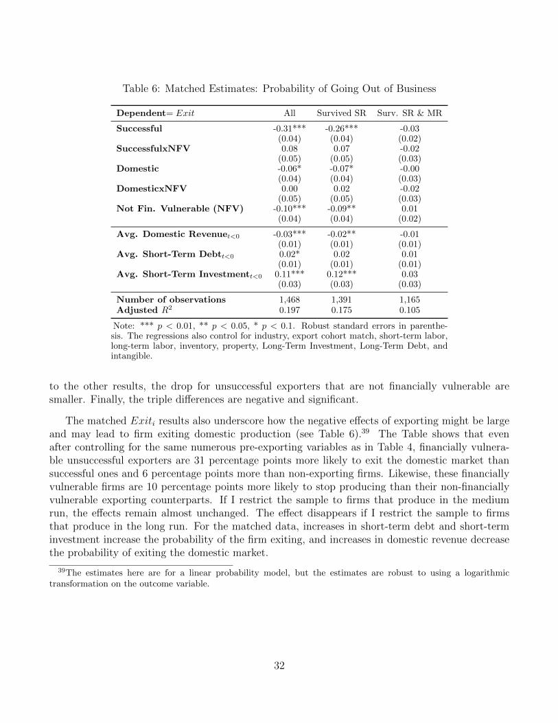
Table 6: Matched Estimates: Probability of Going Out of Business

Dependent= Exit All Survived SR Surv. SR & MR

Successful -0.31*** -0.26*** -0.03(0.04) (0.04) (0.02)

SuccessfulxNFV 0.08 0.07 -0.02(0.05) (0.05) (0.03)

Domestic -0.06* -0.07* -0.00(0.04) (0.04) (0.03)

DomesticxNFV 0.00 0.02 -0.02(0.05) (0.05) (0.03)

Not Fin. Vulnerable (NFV) -0.10*** -0.09** 0.01(0.04) (0.04) (0.02)

Avg. Domestic Revenuet<0 -0.03*** -0.02** -0.01(0.01) (0.01) (0.01)

Avg. Short-Term Debtt<0 0.02* 0.02 0.01(0.01) (0.01) (0.01)

Avg. Short-Term Investmentt<0 0.11*** 0.12*** 0.03(0.03) (0.03) (0.03)

Number of observations 1,468 1,391 1,165Adjusted R2 0.197 0.175 0.105

Note: *** p < 0.01, ** p < 0.05, * p < 0.1. Robust standard errors in parenthe-sis. The regressions also control for industry, export cohort match, short-term labor,long-term labor, inventory, property, Long-Term Investment, Long-Term Debt, andintangible.

to the other results, the drop for unsuccessful exporters that are not financially vulnerable aresmaller. Finally, the triple differences are negative and significant.

The matched Exiti results also underscore how the negative effects of exporting might be largeand may lead to firm exiting domestic production (see Table 6).39 The Table shows that evenafter controlling for the same numerous pre-exporting variables as in Table 4, financially vulnera-ble unsuccessful exporters are 31 percentage points more likely to exit the domestic market thansuccessful ones and 6 percentage points more than non-exporting firms. Likewise, these financiallyvulnerable firms are 10 percentage points more likely to stop producing than their non-financiallyvulnerable exporting counterparts. If I restrict the sample to firms that produce in the mediumrun, the effects remain almost unchanged. The effect disappears if I restrict the sample to firmsthat produce in the long run. For the matched data, increases in short-term debt and short-terminvestment increase the probability of the firm exiting, and increases in domestic revenue decreasethe probability of exiting the domestic market.

39The estimates here are for a linear probability model, but the estimates are robust to using a logarithmictransformation on the outcome variable.

32

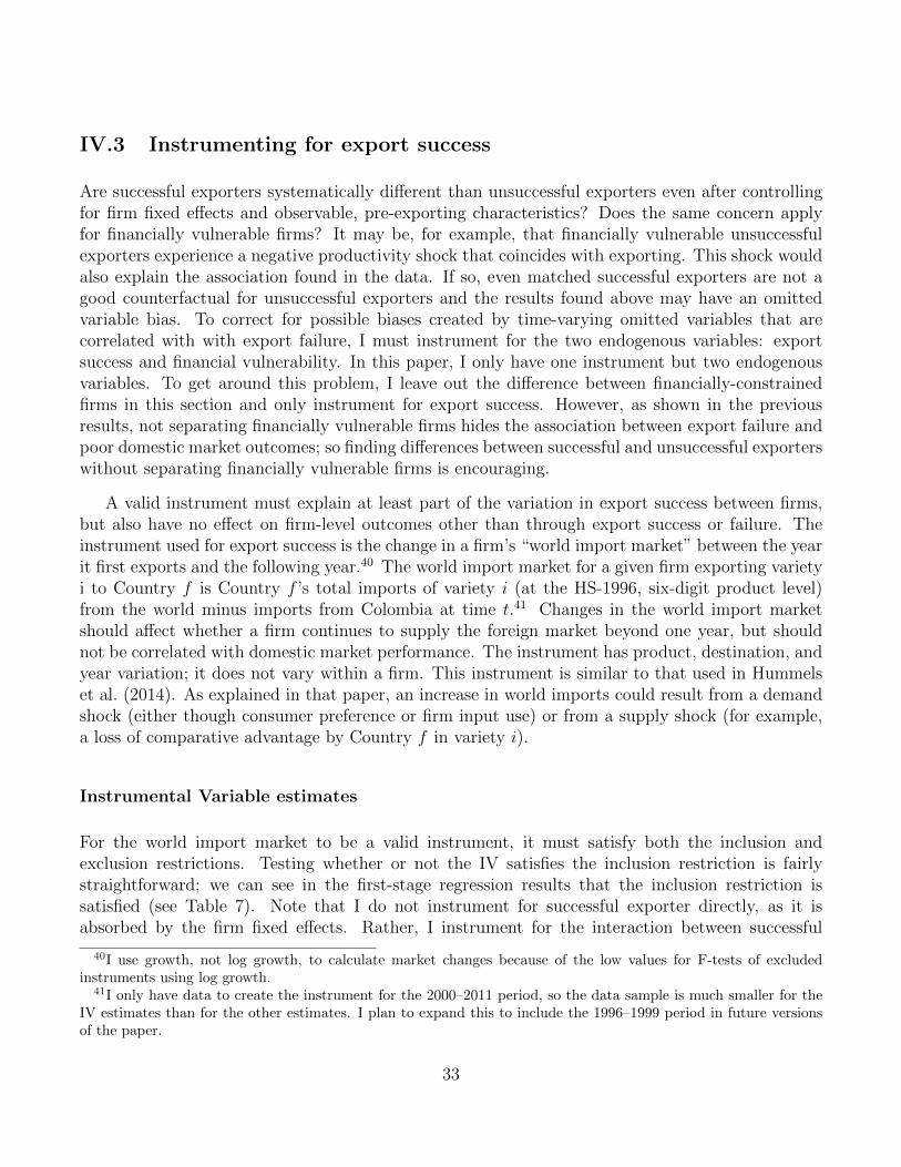
IV.3 Instrumenting for export success

Are successful exporters systematically different than unsuccessful exporters even after controllingfor firm fixed effects and observable, pre-exporting characteristics? Does the same concern applyfor financially vulnerable firms? It may be, for example, that financially vulnerable unsuccessfulexporters experience a negative productivity shock that coincides with exporting. This shock wouldalso explain the association found in the data. If so, even matched successful exporters are not agood counterfactual for unsuccessful exporters and the results found above may have an omittedvariable bias. To correct for possible biases created by time-varying omitted variables that arecorrelated with with export failure, I must instrument for the two endogenous variables: exportsuccess and financial vulnerability. In this paper, I only have one instrument but two endogenousvariables. To get around this problem, I leave out the difference between financially-constrainedfirms in this section and only instrument for export success. However, as shown in the previousresults, not separating financially vulnerable firms hides the association between export failure andpoor domestic market outcomes; so finding differences between successful and unsuccessful exporterswithout separating financially vulnerable firms is encouraging.

A valid instrument must explain at least part of the variation in export success between firms,but also have no effect on firm-level outcomes other than through export success or failure. Theinstrument used for export success is the change in a firm’s “world import market” between the yearit first exports and the following year.40 The world import market for a given firm exporting varietyi to Country f is Country f ’s total imports of variety i (at the HS-1996, six-digit product level)from the world minus imports from Colombia at time t.41 Changes in the world import marketshould affect whether a firm continues to supply the foreign market beyond one year, but shouldnot be correlated with domestic market performance. The instrument has product, destination, andyear variation; it does not vary within a firm. This instrument is similar to that used in Hummelset al. (2014). As explained in that paper, an increase in world imports could result from a demandshock (either though consumer preference or firm input use) or from a supply shock (for example,a loss of comparative advantage by Country f in variety i).

Instrumental Variable estimates

For the world import market to be a valid instrument, it must satisfy both the inclusion andexclusion restrictions. Testing whether or not the IV satisfies the inclusion restriction is fairlystraightforward; we can see in the first-stage regression results that the inclusion restriction issatisfied (see Table 7). Note that I do not instrument for successful exporter directly, as it isabsorbed by the firm fixed effects. Rather, I instrument for the interaction between successful

40I use growth, not log growth, to calculate market changes because of the low values for F-tests of excludedinstruments using log growth.

41I only have data to create the instrument for the 2000–2011 period, so the data sample is much smaller for theIV estimates than for the other estimates. I plan to expand this to include the 1996–1999 period in future versionsof the paper.

33

Table 7: First-Stage Regressions for Market Changes as a Instrument

Dep.→ A(0)*Suc A(1-5)*Suc A(>5)*Suc A(0)*Suc A(1-5)*Suc A(>5)*Suc

A(t = 0) 0.58*** -0.01*** -0.00 0.58*** -0.01*** -0.00*(0.02) (0.00) (0.00) (0.02) (0.00) (0.00)

A(t = 1− 5) 0.01** 0.62*** -0.00 0.01** 0.61*** -0.00(0.00) (0.02) (0.00) (0.00) (0.02) (0.00)

A(rest) 0.01 -0.02 0.76*** 0.00 -0.04** 0.76***(0.00) (0.02) (0.02) (0.01) (0.02) (0.02)

A(t = 0)*IV -0.002*** 0.0002** -0.00002 -0.002*** 0.0002 -0.00002(0.00) (0.00) (0.00) (0.00) (0.00) (0.00)

A(t = 1− 5)*IV 0.0002 -0.00*** -0.00002 0.0001 -0.002*** -0.00003(0.00) (0.00) (0.00) (0.00) (0.00) (0.00)

A(rest)*IV -0.002 -0.01 0.015 -0.002 -0.01 0.02(0.00) (0.01) (0.01) (0.00) (0.01) (0.01)

Observations 10,207 10,207 10,207 9,581 9,581 9,581Adjusted R2 0.542 0.613 0.735 0.542 0.613 0.734

Second-stage ln(Domestic Revenue) Domestic Revenue Growth

Note: *** p < 0.01, ** p < 0.05, * p < 0.1; All regression include firm fixed effects and year fixed effects. Robust standard errors, clusteredat the firm level, in parenthesis. Angrist-Pischke multivariate F test of excluded instruments for Log(dom. Rev.)/ ∆log(dom. Rev.):Successful*(Year of exp) = 48.44/45.27, Successful*After(t=1 to 5) = 12.54/12.04, Successful*After(rest) = 1.1/1.34.

exporter and the three after periods; that is, I instrument for the short-run, medium-run andlong-run difference-in-difference variables. I instrument for these difference-in-difference variablesusing the interactions between the three periods and the instrument for successful exporters; seeWooldridge (2008) for details on the estimation procedure. The first stage regressions have highF-tests and show that export success is indeed correlated with market changes. The Angrist-Pischkemultivariate F-tests for After(t = 0) ∗ Succ., After(t = 1 to 5) ∗ Succ., and After(rest) ∗ Succ.,are about 45, 12, and 1, respectively.42 The first-stage estimates also show that the instrument isoverall significantly correlated with export success and that the correlation decreases both in termsof size and significance for the long-run difference-in-difference estimates.

To satisfy the exclusion restriction, the error term must not be correlated with the changes inforeign markets. It is unlikely that a new exporter can affect market changes in its world importmarket. While the shocks are exogenous to the firm, the exclusion restriction might nonethelessbe violated if there is something about successful exporters that enables them to identify growthopportunities and also enables them to do better in the domestic market. Likewise, there are issueswith the instrument if the world import market is correlated with the domestic market. Since Icontrol for year fixed effect, this is only an issue if the shocks and correlation are industry specific.43

42The F-test differ slightly depending on whether the outcome variables is domestic revenue or domestic revenuegrowth. The reason for this difference is that the number of observations is different depending on the outcomevariable.

43Although not done in this version of the paper, in future versions of this paper, I plan to run separate regressions

34

Table 8: IV Estimates

Dependent→ Ln(Dom. Rev.) ∆Ln(Dom. Rev.)

Year of exp -0.13* -0.31***(0.08) (0.11)

After(t = 1 to 5) -0.66*** -0.60***(0.25) (0.17)

After(rest) 0.23 -0.03(1.88) (0.72)

Successful*Year of exp 0.26* 0.32(0.14) (0.20)

Successful*After(t = 1 to 5) 0.90** 0.74***(0.40) (0.28)

Successful*After(rest) -0.60 -0.16(2.48) (0.96)

Firm and year fixed effects Yes YesNumber of observations 10,207 9,581Number of clusters/groups 904 904

Note: *** p < 0.01, ** p < 0.05, * p < 0.1; All regression include firm fixed effects andyear fixed effects. Robust standard errors, clustered at the firm level, in parenthesis.

For example, a positive shock to industry producers in the rest of the world may make domesticfirms less likely to continue exporting in a foreign country and also to experience a negative shockin the home market. Another problem not addressed by this instrument is that exporting mightbe associated with learning-by-doing; if learning-by-exporting exists—something that is disputed—export success would cause better domestic market performance and focusing on the difference-in-difference estimate to test the effects of export failure is not appropriate.

After instrumenting for successful exporters, as can be see in Table 8, much of the differencebetween successful and unsuccessful exporters in the first year of exporting disappears. This mightbe expected since in that period both types of firms export; the difference should be seen afterexport success is determined, in the medium and long run.44 I find that indeed in the mediumrun, there is a significant difference between successful and unsuccessful exporters. In those years,unsuccessful exporters, relative to successful ones, have much lower domestic revenue and domesticrevenue growth. There are no statistically significant differences in the long run.

Finally, the significance of the results using Exit as a dependent variable also do not change if Iuse an instrumental variable approach. Unsuccessful exporters are more likely to exit the domesticmarket than successful ones, but this difference disappears if the firm manages to survive beyondthe medium run (see Table 9).

within industries to see if my result are sensitive to firm industries.44Alternatively we might expect there to be a difference in the short run; while no firm has “failed” at exporting

in this period, some firms might be in the process of failing.

35

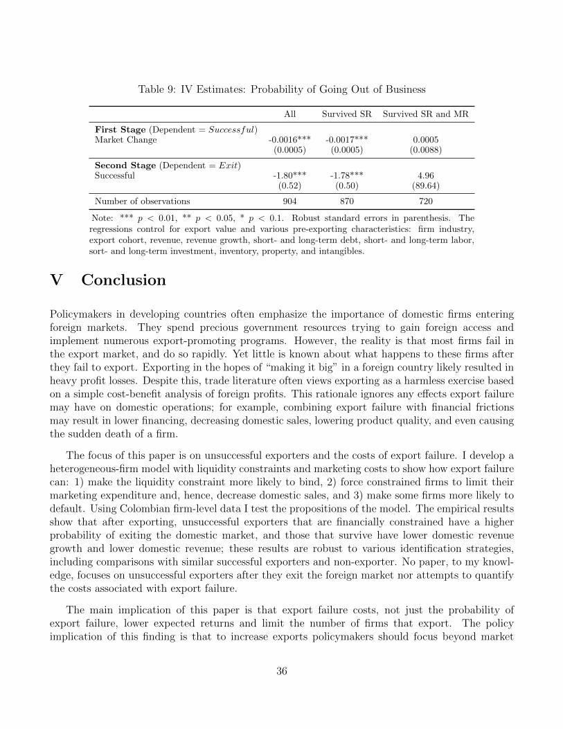
Table 9: IV Estimates: Probability of Going Out of Business

All Survived SR Survived SR and MR

First Stage (Dependent = Successful)Market Change -0.0016*** -0.0017*** 0.0005

(0.0005) (0.0005) (0.0088)

Second Stage (Dependent = Exit)Successful -1.80*** -1.78*** 4.96

(0.52) (0.50) (89.64)

Number of observations 904 870 720

Note: *** p < 0.01, ** p < 0.05, * p < 0.1. Robust standard errors in parenthesis. Theregressions control for export value and various pre-exporting characteristics: firm industry,export cohort, revenue, revenue growth, short- and long-term debt, short- and long-term labor,sort- and long-term investment, inventory, property, and intangibles.

V Conclusion

Policymakers in developing countries often emphasize the importance of domestic firms enteringforeign markets. They spend precious government resources trying to gain foreign access andimplement numerous export-promoting programs. However, the reality is that most firms fail inthe export market, and do so rapidly. Yet little is known about what happens to these firms afterthey fail to export. Exporting in the hopes of “making it big” in a foreign country likely resulted inheavy profit losses. Despite this, trade literature often views exporting as a harmless exercise basedon a simple cost-benefit analysis of foreign profits. This rationale ignores any effects export failuremay have on domestic operations; for example, combining export failure with financial frictionsmay result in lower financing, decreasing domestic sales, lowering product quality, and even causingthe sudden death of a firm.

The focus of this paper is on unsuccessful exporters and the costs of export failure. I develop aheterogeneous-firm model with liquidity constraints and marketing costs to show how export failurecan: 1) make the liquidity constraint more likely to bind, 2) force constrained firms to limit theirmarketing expenditure and, hence, decrease domestic sales, and 3) make some firms more likely todefault. Using Colombian firm-level data I test the propositions of the model. The empirical resultsshow that after exporting, unsuccessful exporters that are financially constrained have a higherprobability of exiting the domestic market, and those that survive have lower domestic revenuegrowth and lower domestic revenue; these results are robust to various identification strategies,including comparisons with similar successful exporters and non-exporter. No paper, to my knowl-edge, focuses on unsuccessful exporters after they exit the foreign market nor attempts to quantifythe costs associated with export failure.

The main implication of this paper is that export failure costs, not just the probability ofexport failure, lower expected returns and limit the number of firms that export. The policyimplication of this finding is that to increase exports policymakers should focus beyond market

36

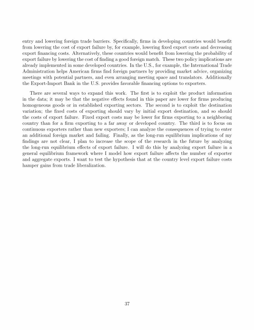
entry and lowering foreign trade barriers. Specifically, firms in developing countries would benefitfrom lowering the cost of export failure by, for example, lowering fixed export costs and decreasingexport financing costs. Alternatively, these countries would benefit from lowering the probability ofexport failure by lowering the cost of finding a good foreign match. These two policy implications arealready implemented in some developed countries. In the U.S., for example, the International TradeAdministration helps American firms find foreign partners by providing market advice, organizingmeetings with potential partners, and even arranging meeting space and translators. Additionallythe Export-Import Bank in the U.S. provides favorable financing options to exporters.

There are several ways to expand this work. The first is to exploit the product informationin the data; it may be that the negative effects found in this paper are lower for firms producinghomogeneous goods or in established exporting sectors. The second is to exploit the destinationvariation; the fixed costs of exporting should vary by initial export destination, and so shouldthe costs of export failure. Fixed export costs may be lower for firms exporting to a neighboringcountry than for a firm exporting to a far away or developed country. The third is to focus oncontinuous exporters rather than new exporters; I can analyze the consequences of trying to enteran additional foreign market and failing. Finally, as the long-run equilibrium implications of myfindings are not clear, I plan to increase the scope of the research in the future by analyzingthe long-run equilibrium effects of export failure. I will do this by analyzing export failure in ageneral equilibrium framework where I model how export failure affects the number of exporterand aggregate exports. I want to test the hypothesis that at the country level export failure costshamper gains from trade liberalization.

37

References

Ahn, JaeBin and Alexander F. McQuoid (2013), “Capacity constrained exporters: Micro evidenceand macro implications.”

Albornoz, Facundo, Hector F. Calvo Pardo, Gregory Corcos, and Emanuel Ornelas (2012), “Se-quential exporting.” Journal of International Economics, 88, 17–31.

Alessandria, George, Joseph P. Kaboski, and Virgiliu Midrigan (2010), “Inventories, lumpy trade,and large devaluations.” The American Economic Review, 100, 2304–2339.

Amiti, Mary and David E. Weinstein (2011), “Exports and financial shocks.” The Quarterly Journalof Economics, 126, 1841–1877.

Antunes, Antonio, Luca Opromolla, and Katheryn Russ (2014), “Dissecting risk: Exit, default, andexport participation.”

Arkolakis, Costas (2010), “Market penetration costs and the new consumers margin in internationaltrade.” Journal of Political Economy, 118, pp. 1151–1199.

Bernard, Andrew B. and J. Bradford Jensen (2004), “Why some firms export.” Review of Economicsand Statistics, 86, 561–569.

Bernard, Andrew B., J. Bradford Jensen, Stephen J. Redding, and Peter K. Schott (2007), “Firmsin international trade.” The Journal of Economic Perspectives, 105–130.

Bernard, Andrew B., Stephen J. Redding, and Peter K. Schott (2011), “Multiproduct firms andtrade liberalization.” The Quarterly Journal of Economics, 126, 1271–1318.

Besedes, Tibor and Thomas J. Prusa (2006a), “Ins, outs, and the duration of trade.” The CanadianJournal of Economics / Revue canadienne d’Economique, 39, pp. 266–295.

Besedes, Tibor and Thomas J. Prusa (2006b), “Product differentiation and duration of US importtrade.” Journal of International Economics, 70, 339–358.

Besedes, Tibor and Thomas J. Prusa (2011), “The role of extensive and intensive margins andexport growth.” Journal of Development Economics, 96, 371–379.

Blum, Bernardo S., Sebastian Claro, and Ignatius J. Horstmann (2013), “Occasional and perennialexporters.” Journal of International Economics, 90, 65–74.

Brooks, Eileen L. (2006), “Why don’t firms export more? product quality and Colombian plants.”Journal of Development Economics, 80, 160–178.

Bustos, Paula (2011), “Trade liberalization, exports, and technology upgrading: Evidence on theimpact of MERCOSUR on Argentinian firms.” The American Economic Review, 101, 304–340.

38

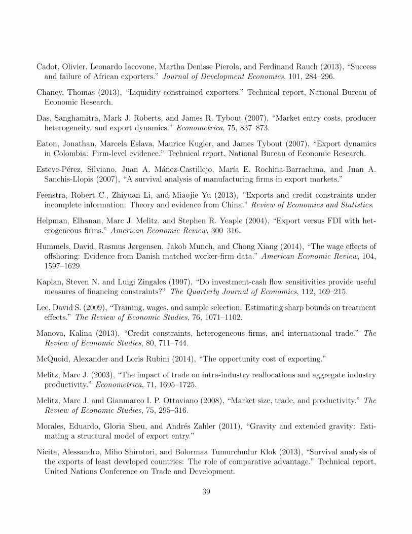
Cadot, Olivier, Leonardo Iacovone, Martha Denisse Pierola, and Ferdinand Rauch (2013), “Successand failure of African exporters.” Journal of Development Economics, 101, 284–296.

Chaney, Thomas (2013), “Liquidity constrained exporters.” Technical report, National Bureau ofEconomic Research.

Das, Sanghamitra, Mark J. Roberts, and James R. Tybout (2007), “Market entry costs, producerheterogeneity, and export dynamics.” Econometrica, 75, 837–873.

Eaton, Jonathan, Marcela Eslava, Maurice Kugler, and James Tybout (2007), “Export dynamicsin Colombia: Firm-level evidence.” Technical report, National Bureau of Economic Research.

Esteve-Perez, Silviano, Juan A. Manez-Castillejo, Marıa E. Rochina-Barrachina, and Juan A.Sanchis-Llopis (2007), “A survival analysis of manufacturing firms in export markets.”

Feenstra, Robert C., Zhiyuan Li, and Miaojie Yu (2013), “Exports and credit constraints underincomplete information: Theory and evidence from China.” Review of Economics and Statistics.

Helpman, Elhanan, Marc J. Melitz, and Stephen R. Yeaple (2004), “Export versus FDI with het-erogeneous firms.” American Economic Review, 300–316.

Hummels, David, Rasmus Jørgensen, Jakob Munch, and Chong Xiang (2014), “The wage effects ofoffshoring: Evidence from Danish matched worker-firm data.” American Economic Review, 104,1597–1629.

Kaplan, Steven N. and Luigi Zingales (1997), “Do investment-cash flow sensitivities provide usefulmeasures of financing constraints?” The Quarterly Journal of Economics, 112, 169–215.

Lee, David S. (2009), “Training, wages, and sample selection: Estimating sharp bounds on treatmenteffects.” The Review of Economic Studies, 76, 1071–1102.

Manova, Kalina (2013), “Credit constraints, heterogeneous firms, and international trade.” TheReview of Economic Studies, 80, 711–744.

McQuoid, Alexander and Loris Rubini (2014), “The opportunity cost of exporting.”

Melitz, Marc J. (2003), “The impact of trade on intra-industry reallocations and aggregate industryproductivity.” Econometrica, 71, 1695–1725.

Melitz, Marc J. and Gianmarco I. P. Ottaviano (2008), “Market size, trade, and productivity.” TheReview of Economic Studies, 75, 295–316.

Morales, Eduardo, Gloria Sheu, and Andres Zahler (2011), “Gravity and extended gravity: Esti-mating a structural model of export entry.”

Nicita, Alessandro, Miho Shirotori, and Bolormaa Tumurchudur Klok (2013), “Survival analysis ofthe exports of least developed countries: The role of comparative advantage.” Technical report,United Nations Conference on Trade and Development.

39

Rauch, James E and Joel Watson (2003), “Starting small in an unfamiliar environment.” Interna-tional Journal of Industrial Organization, 21, 1021–1042.

Rho, Young-Woo and Joel Rodrigue (2010), “The opportunity cost of exporting.”

Rosenbaum, Paul R. and Donald B. Rubin (1983), “The central role of the propensity score inobservational studies for causal effects.” Biometrika, 70, 41–55.

Smeets, Roger, Harold Creusen, Arjan Lejour, and Henk Kox (2010), “Export margins and exportbarriers: Uncovering market entry costs of exporters in the Netherlands.”

Soderbery, Anson (2014), “Market size, structure, and access: Trade with capacity constraints.”European Economic Review.

Spearot, Alan (2013), “Market access, investment, and heterogeneous firms.” International Eco-nomic Review, 54, 601–627.

Stirbat, Liviu, Richard Record, and Konesawang Nghardsaysone (2013), “Determinants of exportsurvival in the Lao PDR.”

Tovar, Jorge Andres and Luis Roberto Martınez (2011), “Diversification, networks and the survivalof exporting firms.”

Ucbasaran, Deniz, Dean A. Shepherd, Andy Lockett, and S. John Lyon (2013), “Life after businessfailure the process and consequences of business failure for entrepreneurs.” Journal of Manage-ment, 39, 163–202.

Verhoogen, Eric A. (2008), “Trade, quality upgrading, and wage inequality in the Mexican manu-facturing sector.” The Quarterly Journal of Economics, 123, 489–530.

Whited, Toni M. and Guojun Wu (2006), “Financial constraints risk.” Review of Financial Studies,19, 531–559.

Wooldridge, Jeffrey M. (2008), “Instrumental variables estimation of the average treatment effectin the correlated random coefficient model.” Advances in Econometrics, 21, 93–116.

40

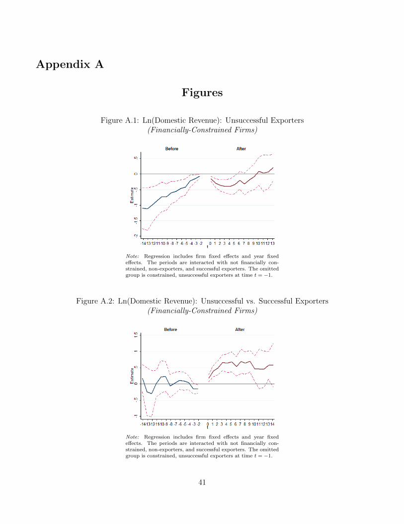
Appendix A

Figures

Figure A.1: Ln(Domestic Revenue): Unsuccessful Exporters(Financially-Constrained Firms)

Note: Regression includes firm fixed effects and year fixedeffects. The periods are interacted with not financially con-strained, non-exporters, and successful exporters. The omittedgroup is constrained, unsuccessful exporters at time t = −1.

Figure A.2: Ln(Domestic Revenue): Unsuccessful vs. Successful Exporters(Financially-Constrained Firms)

Note: Regression includes firm fixed effects and year fixedeffects. The periods are interacted with not financially con-strained, non-exporters, and successful exporters. The omittedgroup is constrained, unsuccessful exporters at time t = −1.

41

Figure A.3: Ln(Domestic Revenue): Unsuccessful Exporters vs. Non-Exporters(Financially-Constrained Firms)

Note: Regression includes firm fixed effects and year fixed effects. The periodsare interacted with not financially constrained, non-exporters, and successful ex-porters. The omitted group is constrained, unsuccessful exporters at time t = −1.

Figure A.4: ∆Ln(Dom. Revenue) for Unsuccessful Exporters(Financially-Constrained Firms)

Note: Regression includes firm fixed effects and year fixed effects. The periodsare interacted with not financially constrained, non-exporters, and successful ex-porters. The omitted group is constrained, unsuccessful exporters at time t = −1.

42

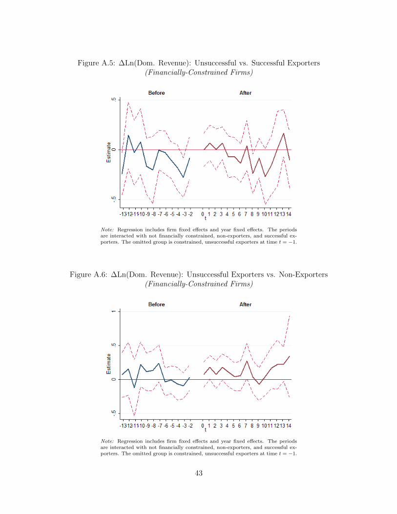
Figure A.5: ∆Ln(Dom. Revenue): Unsuccessful vs. Successful Exporters(Financially-Constrained Firms)

Note: Regression includes firm fixed effects and year fixed effects. The periodsare interacted with not financially constrained, non-exporters, and successful ex-porters. The omitted group is constrained, unsuccessful exporters at time t = −1.

Figure A.6: ∆Ln(Dom. Revenue): Unsuccessful Exporters vs. Non-Exporters(Financially-Constrained Firms)

Note: Regression includes firm fixed effects and year fixed effects. The periodsare interacted with not financially constrained, non-exporters, and successful ex-porters. The omitted group is constrained, unsuccessful exporters at time t = −1.

43

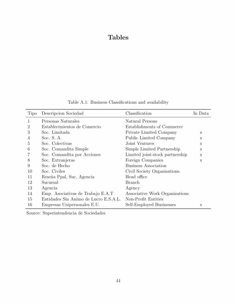
Tables

Table A.1: Business Classifications and availability

Tipo Descripcion Sociedad Classification In Data

1 Personas Naturales Natural Persons2 Establecimientos de Comercio Establishments of Commerce3 Soc. Limitada Private Limited Company x4 Soc. S. A. Public Limited Company x5 Soc. Colectivas Joint Ventures x6 Soc. Comandita Simple Simple Limited Partnership x7 Soc. Comandita por Acciones Limited joint-stock partnership x8 Soc. Extranjeras Foreign Companies x9 Soc. de Hecho Business Association10 Soc. Civiles Civil Society Organisations.11 Resena Ppal, Suc, Agencia Head office12 Sucursal Branch13 Agencia Agency14 Emp. Asociativas de Trabajo E.A.T Associative Work Organizations15 Entidades Sin Animo de Lucro E.S.A.L. Non-Profit Entities16 Empresas Unipersonales E.U. Self-Employed Businesses x

Source: Superintendencia de Sociedades

44

Table A.2: Summary Statistics

Continuous Successful Unsuccessful Non-exporters

Trade dataAvg. Number of Exporters per Year 2,458 4,242 1,817 -Share of Exporters 0.30 0.52 0.22 -Share Export value 0.74 0.27 0.01 -Share of New Exporters - 0.36 0.64 -Share New Export value - 0.68 0.32 -

Financial DataAvg. Number of Firms per Year 1,887 1,964 706 10,803Share of Firms 0.12 0.13 0.05 0.70Revenue (1 billion COL Pesos) 49.3 26.6 14.9 6.0Exports(1 billion COL Pesos) 11.3 3.8 0.1 -Exports/Revenue 0.23 0.14 0.00 -

Note: Calculations based on data from the Colombian National Directorate of Taxes and Customs(DIAN) and Superintendencia de Sociedades.

45

Table A.3: PPML Estimates: Check Balance on Variables

Explanatory Variable = All Periods One PeriodSuccessful Exporter Before Exporting Before Exporting

Short-Term Debt 0.17 0.17(0.39) (0.29)

Long-Term Debt 0.17 -0.35(0.29) (0.23)

Short-Term Labor 0.20 0.02(0.16) (0.14)

Long-Term Labor -0.25 0.11(0.68) (0.41)

Sort-Term Investment 0.13 0.07(0.34) (0.31)

Long-Term Investment 0.77** 0.72**(0.36) (0.33)

Inventory 0.33 0.11(0.23) (0.19)

Property -0.10 -0.27(0.43) (0.35)

Intangibles 0.54 0.10(0.48) (0.46)

Total Observations 6,018 1,239

Note: *** p < 0.01, ** p < 0.05, * p < 0.1; standard errors,clustered at the firm level, shown in parenthesis. Outcome vari-ables are listed on the left, so the table displays the estimateson the ”successful (future) exporter” variable. All regressions areperformed by PPML2 (Poisson pseudo-maximum likelihood).

46

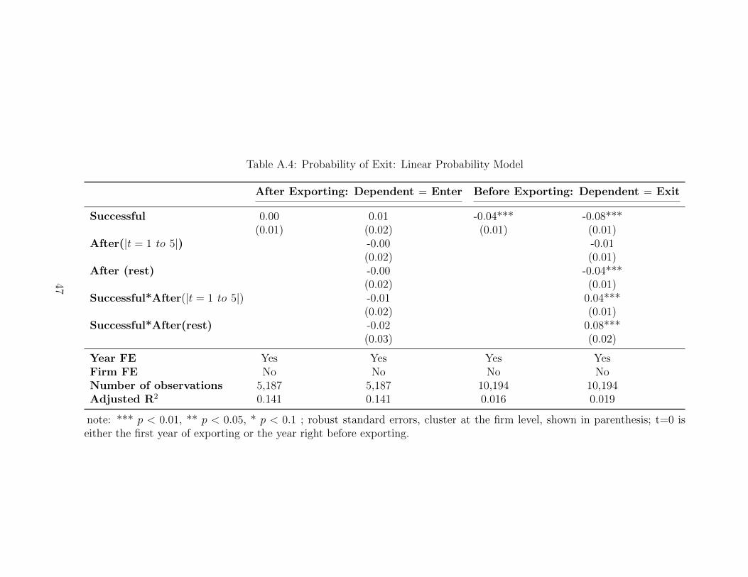
Table A.4: Probability of Exit: Linear Probability Model

After Exporting: Dependent = Enter Before Exporting: Dependent = Exit

Successful 0.00 0.01 -0.04*** -0.08***(0.01) (0.02) (0.01) (0.01)

After(|t = 1 to 5|) -0.00 -0.01(0.02) (0.01)

After (rest) -0.00 -0.04***(0.02) (0.01)

Successful*After(|t = 1 to 5|) -0.01 0.04***(0.02) (0.01)

Successful*After(rest) -0.02 0.08***(0.03) (0.02)

Year FE Yes Yes Yes YesFirm FE No No No NoNumber of observations 5,187 5,187 10,194 10,194Adjusted R2 0.141 0.141 0.016 0.019

note: *** p < 0.01, ** p < 0.05, * p < 0.1 ; robust standard errors, cluster at the firm level, shown in parenthesis; t=0 iseither the first year of exporting or the year right before exporting.

47

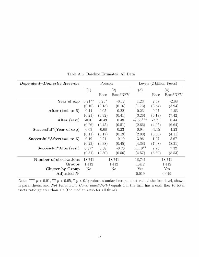
Table A.5: Baseline Estimates: All Data

Dependent=Domestic Revenue Poisson Levels (2 billion Pesos)

(1) (2) (3) (4)Base Base*NFV Base Base*NFV

Year of exp 0.21** 0.25* -0.12 1.23 2.57 -2.88(0.10) (0.15) (0.16) (1.73) (3.54) (3.94)

After (t=1 to 5) 0.14 0.05 0.22 0.23 0.97 -1.63(0.21) (0.32) (0.41) (3.26) (6.18) (7.42)

After (rest) -0.31 -0.49 0.48 -7.66*** -7.71 0.44(0.26) (0.45) (0.51) (2.66) (4.95) (6.64)

Successful*(Year of exp) 0.03 -0.08 0.23 0.94 -1.15 4.23(0.11) (0.17) (0.19) (2.00) (3.80) (4.11)

Successful*After(t=1 to 5) 0.19 0.21 -0.10 3.96 1.07 5.67(0.23) (0.38) (0.45) (4.38) (7.08) (8.31)

Successful*After(rest) 0.57* 0.58 -0.20 11.10** 7.25 7.32(0.31) (0.50) (0.56) (4.57) (6.59) (8.53)

Number of observations 18,741 18,741 18,741 18,741Groups 1,412 1,412 1,412 1,412

Cluster by Group No No Yes YesAdjusted R2 0.019 0.019

Note: *** p < 0.01, ** p < 0.05, * p < 0.1; robust standard errors, clustered at the firm level, shownin parenthesis; and Not Financially Constrained(NFV) equals 1 if the firm has a cash flow to totalassets ratio greater than .07 (the median ratio for all firms).

48

Table A.6: Baseline Estimates: Dropping Firms with Revenues above 1 trillion or More Pesos

Dependent=Domestic Revenue Poisson Levels (2 billion Pesos)

(1) (2) (3) (4)Base Base*NFV Base Base*NFV

Base Base*NFV Base Base*NFVYear of exp 0.07 0.01 0.11 -0.69 -1.28* 1.08

(0.05) (0.07) (0.08) (0.62) (0.66) (0.84)After (t=1 to 5) -0.07 -0.50*** 0.80*** -2.87* -5.51*** 5.53*

(0.19) (0.18) (0.29) (1.62) (1.25) (2.96)After (rest) -0.57*** -1.12*** 1.17*** -9.84*** -12.80*** 6.91***

(0.22) (0.27) (0.33) (1.98) (2.07) (2.54)Successful*(Year of exp) 0.15** 0.15 -0.03 2.56*** 2.36* 0.31

(0.06) (0.10) (0.12) (0.86) (1.24) (1.65)Successful*After(t=1 to 5) 0.36* 0.75*** -0.76** 5.51*** 7.20*** -3.88

(0.20) (0.25) (0.34) (2.06) (2.79) (4.04)Successful*After(rest) 0.78*** 1.23*** -1.02*** 12.16*** 12.97*** -2.74

(0.23) (0.31) (0.38) (2.28) (2.83) (4.50)

Number of observations 18,718 18,718 18,718 18,718Groups 1,410 1,410 1,410 1,410

Cluster by Group No No Yes YesAdjusted R2 0.040 0.042

Note: *** p < 0.01, ** p < 0.05, * p < 0.1; robust standard errors, clustered at the firm level, shown inparenthesis; and Not Financially Constrained(NFV) equals 1 if the firm has a cash flow to total assets ratiogreater than .07 (the median ratio for all firms).

49

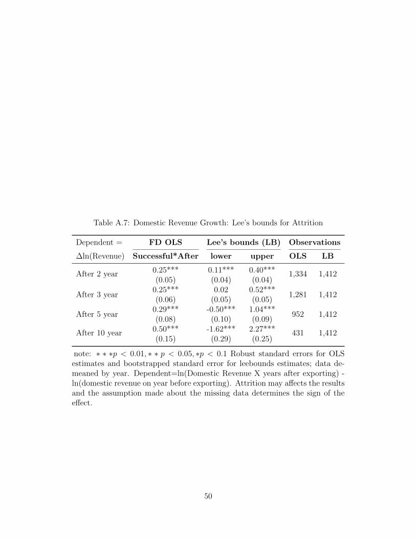
Table A.7: Domestic Revenue Growth: Lee’s bounds for Attrition

Dependent = FD OLS Lee’s bounds (LB) Observations

∆ln(Revenue) Successful*After lower upper OLS LB

After 2 year 0.25*** 0.11*** 0.40*** 1,334 1,412(0.05) (0.04) (0.04)

After 3 year0.25*** 0.02 0.52***

1,281 1,412(0.06) (0.05) (0.05)

After 5 year0.29*** -0.50*** 1.04***

952 1,412(0.08) (0.10) (0.09)

After 10 year 0.50*** -1.62*** 2.27*** 431 1,412(0.15) (0.29) (0.25)

note: ∗ ∗ ∗p < 0.01, ∗ ∗ p < 0.05, ∗p < 0.1 Robust standard errors for OLSestimates and bootstrapped standard error for leebounds estimates; data de-meaned by year. Dependent=ln(Domestic Revenue X years after exporting) -ln(domestic revenue on year before exporting). Attrition may affects the resultsand the assumption made about the missing data determines the sign of theeffect.

50

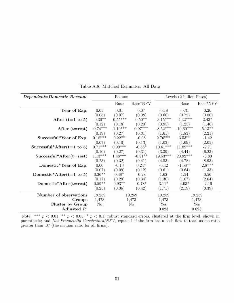
Table A.8: Matched Estimates: All Data

Dependent=Domestic Revenue Poisson Levels (2 billion Pesos)

Base Base*NFV Base Base*NFV

Year of Exp. 0.05 0.01 0.07 -0.18 -0.31 0.20(0.05) (0.07) (0.08) (0.60) (0.72) (0.80)

After (t=1 to 5) -0.30** -0.55*** 0.50** -3.15*** -4.32*** 2.43*(0.12) (0.18) (0.20) (0.95) (1.25) (1.46)

After (t=rest) -0.74*** -1.19*** 0.97*** -8.52*** -10.60*** 5.13**(0.19) (0.27) (0.31) (1.61) (1.83) (2.21)

Successful*Year of Exp. 0.18*** 0.22** -0.08 2.76*** 3.53** -1.42(0.07) (0.10) (0.13) (1.03) (1.69) (2.05)

Successful*After(t=1 to 5) 0.71*** 0.99*** -0.58* 10.61*** 11.89*** -2.71(0.16) (0.27) (0.31) (3.39) (4.44) (6.23)

Successful*After(t=rest) 1.13*** 1.48*** -0.81** 19.53*** 20.92*** -3.83(0.23) (0.32) (0.41) (4.53) (4.78) (8.93)

Domestic*Year of Exp. 0.00 -0.13 0.24* -0.42 -1.58** 2.87**(0.07) (0.09) (0.12) (0.61) (0.64) (1.33)

Domestic*After(t=1 to 5) 0.36** 0.48* -0.28 1.62 1.54 0.56(0.17) (0.29) (0.34) (1.30) (1.67) (2.64)

Domestic*After(t=rest) 0.59** 0.93** -0.78* 3.11* 4.03* -2.16(0.25) (0.36) (0.42) (1.71) (2.19) (3.39)

Number of observations 19,259 19,259 19,259 19,259Groups 1,473 1,473 1,473 1,473

Cluster by Group No No Yes YesAdjusted R2 0.023 0.023

Note: *** p < 0.01, ** p < 0.05, * p < 0.1; robust standard errors, clustered at the firm level, shown inparenthesis; and Not Financially Constrained(NFV) equals 1 if the firm has a cash flow to total assets ratiogreater than .07 (the median ratio for all firms).

51

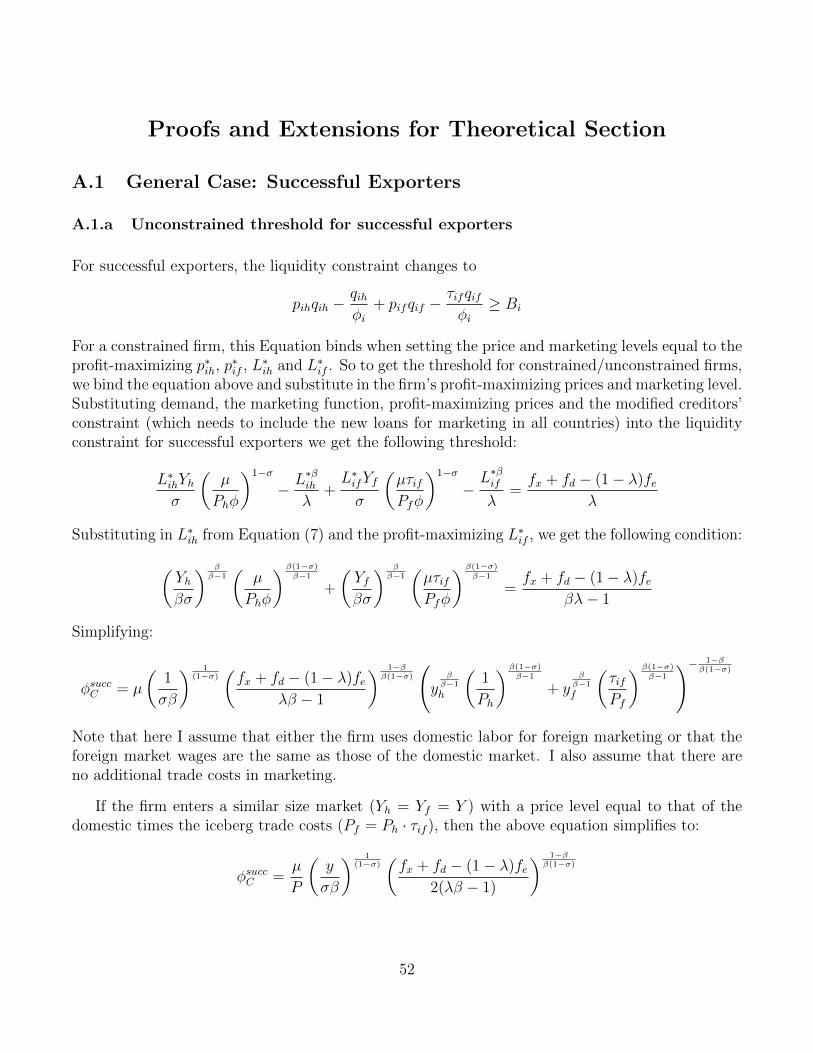
Proofs and Extensions for Theoretical Section

A.1 General Case: Successful Exporters

A.1.a Unconstrained threshold for successful exporters

For successful exporters, the liquidity constraint changes to

pihqih −qihφi

+ pifqif −τifqifφi≥ Bi

For a constrained firm, this Equation binds when setting the price and marketing levels equal to theprofit-maximizing p∗ih, p

∗if , L

∗ih and L∗

if . So to get the threshold for constrained/unconstrained firms,we bind the equation above and substitute in the firm’s profit-maximizing prices and marketing level.Substituting demand, the marketing function, profit-maximizing prices and the modified creditors’constraint (which needs to include the new loans for marketing in all countries) into the liquidityconstraint for successful exporters we get the following threshold:

L∗ihYhσ

(µ

Phφ

)1−σ

− L∗βih

λ+L∗ifYf

σ

(µτifPfφ

)1−σ

−L∗βif

λ=fx + fd − (1− λ)fe

λ

Substituting in L∗ih from Equation (7) and the profit-maximizing L∗

if , we get the following condition:

(Yhβσ

) ββ−1(

µ

Phφ

)β(1−σ)β−1

+

(Yfβσ

) ββ−1(µτifPfφ

)β(1−σ)β−1

=fx + fd − (1− λ)fe

βλ− 1

Simplifying:

φsuccC = µ

(1

σβ

) 1(1−σ)

(fx + fd − (1− λ)fe

λβ − 1

) 1−ββ(1−σ)

(y

ββ−1

h

(1

Ph

)β(1−σ)β−1

+ yββ−1

f

(τifPf

)β(1−σ)β−1

)− 1−ββ(1−σ)

Note that here I assume that either the firm uses domestic labor for foreign marketing or that theforeign market wages are the same as those of the domestic market. I also assume that there areno additional trade costs in marketing.

If the firm enters a similar size market (Yh = Yf = Y ) with a price level equal to that of thedomestic times the iceberg trade costs (Pf = Ph · τif ), then the above equation simplifies to:

φsuccC =µ

P

(y

σβ

) 1(1−σ)

(fx + fd − (1− λ)fe

2(λβ − 1)

) 1−ββ(1−σ)

52

A.1.b Credit-constrained marketing decision for successful exporters

A successful exporter must decide how much to charge for its product and how much to spendon marketing at home and abroad. The prices are not affected by the liquidity constraint, so thefirm always charges the profit maximizing prices in each market. Substituting this price into theexpected profit equation and the modified credit budget constraint into the maximization problem,we get the following:

Max Eπi(pi, Li;φi) =LihYhσ

(µ

Phφ

)1−σ

− Lβih +LifYfσ

(µτifPfφ

)1−σ

− Lβif − fx − fd

Subject to the binding financing constraint:

LihYhσ

(µ

Phφ

)1−σ

− Lβihλ

+LifYfσ

(µτifPfφ

)1−σ

−Lβifλ≥(fx + fd − (1− λ)fe

λ

)Using ε as the multiplier, we get:

∂πi∂ε

:σβLβ−1

ih

Yh

(µ

Phφi

)1−σ =1 + ε

1 + ελ

∂πi∂ε

:σβLβ−1

if

Yf

(µτifPfφi

)1−σ =1 + ε

1 + ελ

∂πi∂ε

:LihYhσ

(µ

Phφ

)1−σ

− Lβihλ

+LifYfσ

(µτifPfφ

)1−σ

−Lβifλ

=fx + fd − (1− λ)fe

λ

This means that Lif =(YfYh

) 1β−1(PhτifPf

) 1−σβ−1

Lih. Substituting Lif out of the financial constraint:

(LihYhσ

(µ

Phφ

)1−σ

− Lβihλ

)(1 +

(YfYh

) ββ−1(PhτifPf

)β(1−σ)β−1

)=fx + fd − (1− λ)fe

λ

Thus, the firm chooses the Lih that solves the following equation:

LihYhσ

(µ

Phφ

)1−σ

− Lβihλ

=

(1 +

(YfYh

) ββ−1(PhτifPf

)β(1−σ)β−1

)−1

fx + fd − (1− λ)feλ

If the firm enters a similar size market (Yh = Yf = Y ) with a price level equal to that of the

53

domestic times the iceberg trade costs (Pf = Ph · τif ), then the above equation simplifies to:

LihYhσ

(µ

Phφ

)1−σ

− Lβihλ

=fx + fd − (1− λ)fe

2λ

A.1.c Firm production threshold for successful exporters

The firm production threshold for successful exporters does not change. All firms want to supplyboth markets and no firm would enter the export market if it knew that, conditional on survivingin the export market, it would have to exit the domestic market.

A.2 Proof of Proposition 1

Proof for the first statement:

We can think of the cutoff for non-exporters as the cutoff before a firm attempts to exports, irre-spective of export success. Thus, to prove the first part of the proposition, I compare, individually,successful and unsuccessful exporters with non-exporters.

To prove that the threshold for unsuccessful exporters is higher after the export attempt (φdomC <φfailC ), Equation (8) must be bigger than Equation (9). This holds as long as fx > 0. Notice alsothat the threshold is higher the higher the fx (∂φC

∂fx> 0). The sign of the derivative is positive

because 1−ββ(1−σ)

> 0, since β > 1 is required for an interior marketing solution and σ > 1 is required

for an interior pricing solution; and, by Assumption 1, we have that fx + fd > (1−λ)fe and λβ > 1.

To prove that the threshold for successful exporters is higher after exporting (φdomC < φsuccC ), weneed Equation (10) to be larger than Equation (9). This holds as long as fd− fx < (1− λ)fe. Thismust hold since (1 − λ)fe > 0 and, by Assumption 2, we have that fx > fd. So some successfulexporters that were not previously constrained might become constrained.

Proof for the second statement:

For the second statement, I compare the thresholds between successful exporters (Equation 10) andunsuccessful exporters (Equation 8). Comparing the two thresholds, we see that φsuccC < φfailC if

1

2(fx + fd − (1− λ)fe) < (fx + fd − (1− λ)fe)

54

This holds because, by Assumption 1, (1 − λ)fe < fx + fd. The difference is decreasing with τif ,holding everything else equal. Thus, the constrained threshold difference between successful andunsuccessful exporters is greatest with smaller iceberg trade costs. The difference between successfuland unsuccessful newly-constrained exporters is that while both are worse off in terms of domesticrevenue, successful exporters are better off overall.

A.3 Proof of that Constrained Li is Increasing in φi

The equations for the constrained Li choice for all firms are identical on the left hand side:LiYσ

(µPφ

)1−σ− Lβi

λ(see Equation 11 for the unsuccessful exporter choice, Equation 12 for the domes-

tic producer choice, and Equation 13 for the successful exporter choice). The right hand side differs,but it does not vary by productivity or marketing choice; changes in productivity only change themarketing choice after export success has been determined. Thus, to prove that the constrained Lichoice is increasing in φi I take the total derivative of each of the equations and set them equal tozero:

dLidφ

=(σ − 1)φσ−2LiY

σ

(µP

)1−σ

βLβ−1i

λ− Y

σ

(µPφ

)1−σ > 0

This is positive since σ − 1 > 0, σ > 1, andβLβ−1

i

λ> Y

σ

(µPφ

)1−σ. Notice that Y

σ

(µPφ

)1−σis the

marginal revenue of marketing andβLβ−1

i

λis the marginal cost of borrowing for marketing costs. All

firms are risk neutral, and all unconstrained firms choose the Li that sets the marginal cost(βLβ−1

i

)equal to the marginal revenue of marketing

(Yσ

(µPφ

)1−σ)

. Marginal cost is below the marginal

cost of borrowing for marketing(βLβ−1

i

λ

). With no financial frictions, λ = 1, the two marginal costs

equal. For unconstrained firms, marginal revenue from marketing is less than the marginal costfrom marketing. Constrained firms would like to do this as well, but doing so makes their liquidityconstraint bind. As they decrease Li, their marginal cost of borrowing for marketing decreases, butit is still above their marginal revenue. Deviating also means lower expected profits, so the firmsdeviate as little as possible. There is no point in lowering Li below LCi , and hence no point inlowering marginal costs below that which equates marginal revenue to marginal cost of borrowingfor marketing. So the last firm to produce is the one that in order to borrow has to set marginalcost of borrowing for marketing equal to marginal revenue of marketing. All firms set marginal cost

of borrowing for marketing greater than or equal to the marginal revenue

(βLβ−1

i

λ≥ Y

σ

(µPφ

)1−σ)

and only unconstrained firms set marginal cost of marketing equal to marginal revenue of marketing(βLβ−1

i = Yσ

(µPφ

)1−σ)

.

55

A.4 Proof of Proposition 2

Proof for the first statement:

We can think of the Li for non-exporters as the Li for successful and unsuccessful exporters beforethey attempted to export. Thus, to prove the first part of the proposition, I compare, individually,successful and unsuccessful exporters with non-exporters.

Since Li is decreasing between the profit-maximizing L∗i and LCi , then ∂LHSi

∂Li< 0 in Equation

(11). Since ∂LHSi∂Li

< 0, to prove that the Li for constrained unsuccessful exporters is lower after

exporting (Ldom > Lfail), I have to show that fd − (1 − λ)fe < fx + fd − (1 − λ)fe. Since 0 < fx,then Ldom > Lfail. Alternatively, we can also note that ∂Li

∂fx< 0. Thus, if ∂RHSi

∂fx> 0 in the same

equation, then ∂Li∂fx

< 0. Taking the derivative of the right hand side with respect to fx, we get∂RHSi∂fx

= 1λ> 0, so ∂Li

∂fx< 0.

Whether or not Li for constrained successful exporters is lower after exporting (Ldom > Lsucc)depends on whether or not the new market loosens or tightens the constrained. If the markets aresimilar, then it is likely that entering the new market tightens the constraint. We can see if the newmarket constrains the successful firm by comparing Equations (12) and (13). For Equation (13), Iassumed the firm enters a similar sized market (Yh = Yf = Y ) with a price level equal to that ofthe domestic times the iceberg trade costs (Pf = Ph · τif ). Then Ldom > Lsucc when

fd − (1− λ)fe <1

2(fx + fd − (1− λ)fe)

That is, when fd − fx < (1− λ)fe. This is likely to be the case, since, by Assumption 2, fd < fx.

Proof for the second statement:

We can prove that the constrained Li is less for unsuccessful than successful exporters (Lfail < Lsucc)from Equation (11) and Equation (13). In those equations we see that successful exporters are betteroff as long as 1

2(fx + fd − (1− λ)fe) < (fx + fd − (1− λ)fe). Which, as we saw in Appendix A.2,

is likely to hold.

A.5 Proof of Proposition 3

Proof for the first statement:

We can think of the production cutoff for non-exporters as the production cutoff for successfuland unsuccessful exporters before the firms attempt to exports. To prove the first statement, I

56

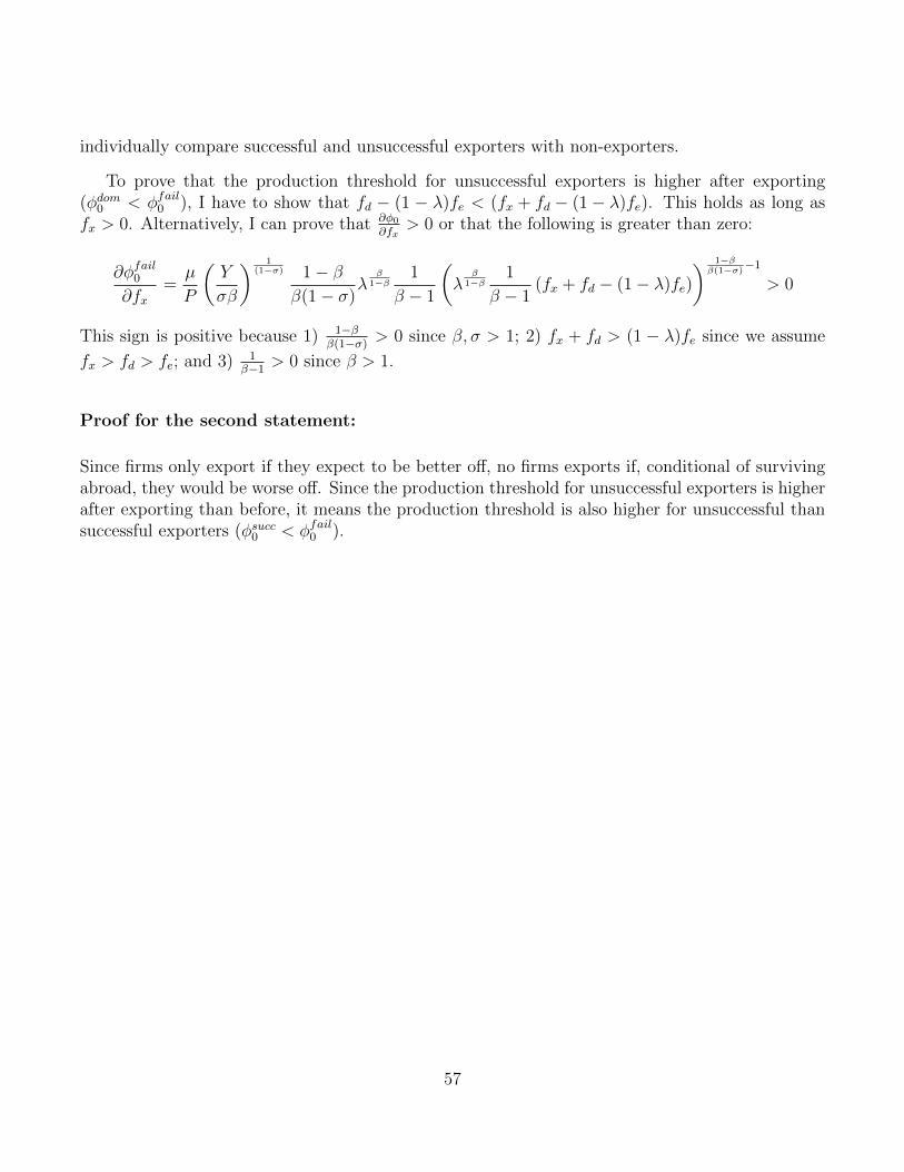
individually compare successful and unsuccessful exporters with non-exporters.

To prove that the production threshold for unsuccessful exporters is higher after exporting(φdom0 < φfail0 ), I have to show that fd − (1 − λ)fe < (fx + fd − (1− λ)fe). This holds as long asfx > 0. Alternatively, I can prove that ∂φ0

∂fx> 0 or that the following is greater than zero:

∂φfail0

∂fx=µ

P

(Y

σβ

) 1(1−σ) 1− β

β(1− σ)λ

β1−β

1

β − 1

(λ

β1−β

1

β − 1(fx + fd − (1− λ)fe)

) 1−ββ(1−σ)−1

> 0

This sign is positive because 1) 1−ββ(1−σ)

> 0 since β, σ > 1; 2) fx + fd > (1 − λ)fe since we assume

fx > fd > fe; and 3) 1β−1

> 0 since β > 1.

Proof for the second statement:

Since firms only export if they expect to be better off, no firms exports if, conditional of survivingabroad, they would be worse off. Since the production threshold for unsuccessful exporters is higherafter exporting than before, it means the production threshold is also higher for unsuccessful thansuccessful exporters (φsucc0 < φfail0 ).

57