1

Exposing Digital Forgeries byDetecting Traces of Re-sampling

Alin C. Popescu and Hany Farid†

Abstract— The unique stature of photographs as a definitiverecording of events is being diminished due, in part, to theease with which digital images can be manipulated and altered.Although good forgeries may leave no visual clues of havingbeen tampered with, they may, nevertheless, alter the underlyingstatistics of an image. For example, we describe how re-sampling(e.g., scaling or rotating) introduces specific statistical correla-tions, and describe how these correlations can be automaticallydetected in any portion of an image. This technique works inthe absence of any digital watermark or signature. We show theefficacy of this approach on uncompressed TIFF images, andJPEG and GIF images with minimal compression. We expectthis technique to be among the first of many tools that will beneeded to expose digital forgeries.

I. INTRODUCTION

With the advent of low-cost and high-resolution digitalcameras, and sophisticated editing software, digital imagescan be easily manipulated and altered. Digital forgeries, oftenleaving no visual clues of having been tampered with, canbe indistinguishable from authentic photographs. As a result,photographs no longer hold the unique stature as a definitiverecording of events. Of particular concern is how the judicialsystem and news media will contend with this issue. Forexample, in March of 2003 the Los Angeles Times published,on its front page, a dramatic photograph of a soldier directingan Iraqi citizen to take cover. The photograph, however, wasa fake - it was digitally created by splicing together twophotographs 1. This and similar incidents naturally lead usto wonder how many of the images that we see every dayhave been digitally doctored.

Digital watermarking has been proposed as a means bywhich an image can be authenticated (see, for example, [1],[2] for general surveys). Within this broad area, several au-thentication schemes have been proposed: embedded signa-tures [3], [4], [5], [6], [7], eraseable fragile watermarks [8],[9], semi-fragile watermarks [10], [11], [12], [13], robusttell-tale watermarks [14], [15], [12], [16], [17], and self-embedding watermarks [18]. All of these approaches work

A. C. Popescu is with the Computer Science Department at DartmouthCollege.

Corresponding author: H. Farid, 6211 Sudikoff Lab, Computer Sci-ence Department, Dartmouth College, Hanover, NH 03755 USA (email:farid@cs.dartmouth.edu; tel/fax: 603.646.2761/603.646.1672). This work wassupported by an Alfred P. Sloan Fellowship, an NSF CAREER Award (IIS-99-83806), an NSF Infrastructure Grant (EIA-98-02068), and under AwardNo. 2000-DT-CX-K001 from the Office for Domestic Preparedness, U.S.Department of Homeland Security (points of view in this document are thoseof the authors and do not necessarily represent the official position of the U.S.Department of Homeland Security).

1The fake was discovered when an editor at The Hartford Courant noticedthat civilians in the background appeared twice in the photo.

by either inserting at the time of recording an imperceptibledigital code (a watermark) into the image, or extracting at thetime of recording a digital code (a signature) from the imageand re-inserting it into the image or image header. With theassumption that digital tampering will alter a watermark (orsignature), an image can be authenticated by verifying that theextracted watermark is the same as that which was inserted.The major drawback of this approach is that a watermark mustbe inserted at precisely the time of recording, which wouldlimit this approach to specially equipped digital cameras. Thismethod also relies on the assumption that the digital watermarkcannot be easily removed and reinserted - it is not yet clearwhether this is a reasonable assumption (e.g., [19]).

In contrast to these approaches, we describe a technique fordetecting traces of digital tampering in the complete absenceof any form of digital watermark or signature. This approachworks on the assumption that although digital forgeries mayleave no visual clues of having been tampered with, they may,nevertheless, alter the underlying statistics of an image. Forexample, consider the creation of a digital forgery that showsa pair of famous movie stars, rumored to have a romanticrelationship, walking hand-in-hand. Such a photograph couldbe created by splicing together individual images of eachmovie star and overlaying the digitally created composite ontoa sunset beach. In order to create a convincing match, it isoften necessary to re-size, rotate, or stretch portions of theimages. This process requires re-sampling the original imageonto a new sampling lattice. Although this re-sampling isoften imperceptible, it introduces specific correlations into theimage, which when detected can be used as evidence of digitaltampering. We describe the form of these correlations, andhow they can be automatically detected in any portion of animage. We show the general effectiveness of this techniqueand analyze its sensitivity and robustness to counter-attacks.

II. RE-SAMPLING

For purposes of exposition we will first describe how andwhere re-sampling introduces correlations in 1-D signals,and how to detect these correlations. The relatively straight-forward generalization to 2-D images is then presented.

A. Re-sampling Signals

Consider a 1-D discretely-sampled signal x[t] with m sam-ples, Fig. 1(a). The number of samples in this signal can beincreased or decreased by a factor p/q to n samples in threesteps [20]:

2

(a)

1 32

(b)

1 128

(c)

1 128

(d)

1 42

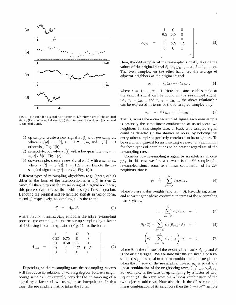
Fig. 1. Re-sampling a signal by a factor of 4/3: shown are (a) the originalsignal; (b) the up-sampled signal; (c) the interpolated signal; and (d) the finalre-sampled signal.

1) up-sample: create a new signal xu[t] with pm samples,where xu[pt] = x[t], t = 1, 2, ...,m, and xu[t] = 0otherwise, Fig. 1(b).

2) interpolate: convolve xu[t] with a low-pass filter: xi[t] =xu[t] ? h[t], Fig. 1(c).

3) down-sample: create a new signal xd[t] with n samples,where xd[t] = xi[qt], t = 1, 2, ..., n. Denote the re-sampled signal as y[t] ≡ xd[t], Fig. 1(d).

Different types of re-sampling algorithms (e.g., linear, cubic)differ in the form of the interpolation filter h[t] in step 2.Since all three steps in the re-sampling of a signal are linear,this process can be described with a single linear equation.Denoting the original and re-sampled signals in vector form,~x and ~y, respectively, re-sampling takes the form:

~y = Ap/q~x, (1)

where the n×m matrix Ap/q embodies the entire re-samplingprocess. For example, the matrix for up-sampling by a factorof 4/3 using linear interpolation (Fig. 1) has the form:

A4/3 =

1 0 0 00.25 0.75 0 00 0.50 0.50 00 0 0.75 0.250 0 0 1

. . .

. (2)

Depending on the re-sampling rate, the re-sampling processwill introduce correlations of varying degrees between neigh-boring samples. For example, consider the up-sampling of asignal by a factor of two using linear interpolation. In thiscase, the re-sampling matrix takes the form:

A2/1 =

1 0 00.5 0.5 00 1 00 0.5 0.50 0 1

. . .

. (3)

Here, the odd samples of the re-sampled signal ~y take on thevalues of the original signal ~x, i.e., y2i−1 = xi, i = 1, . . . , m.The even samples, on the other hand, are the average ofadjacent neighbors of the original signal:

y2i = 0.5xi + 0.5xi+1, (4)

where i = 1, . . . , m − 1. Note that since each sample ofthe original signal can be found in the re-sampled signal,i.e., xi = y2i−1 and xi+1 = y2i+1, the above relationshipcan be expressed in terms of the re-sampled samples only:

y2i = 0.5y2i−1 + 0.5y2i+1. (5)

That is, across the entire re-sampled signal, each even sampleis precisely the same linear combination of its adjacent twoneighbors. In this simple case, at least, a re-sampled signalcould be detected (in the absence of noise) by noticing thatevery other sample is perfectly correlated to its neighbors. Tobe useful in a general forensic setting we need, at a minimum,for these types of correlations to be present regardless of there-sampling rate.

Consider now re-sampling a signal by an arbitrary amountp/q. In this case we first ask, when is the ith sample of are-sampled signal equal to a linear combination of its 2Nneighbors, that is:

yi?=

N∑

k=−N

αkyi+k, (6)

where αk are scalar weights (and α0 = 0). Re-ordering terms,and re-writing the above constraint in terms of the re-samplingmatrix yields:

yi −N∑

k=−N

αkyi+k = 0 (7)

(~ai · ~x) −N∑

k=−N

αk(~ai+k · ~x) = 0 (8)

(

~ai −N∑

k=−N

αk~ai+k

)

· ~x = 0, (9)

where ~ai is the ith row of the re-sampling matrix Ap/q , and ~xis the original signal. We see now that the ith sample of a re-sampled signal is equal to a linear combination of its neighborswhen the ith row of the re-sampling matrix, ~ai, is equal to alinear combination of the neighboring rows,

∑Nk=−N αk~ai+k .

For example, in the case of up-sampling by a factor of two,Equation (3), the even rows are a linear combination of thetwo adjacent odd rows. Note also that if the ith sample is alinear combination of its neighbors then the (i−kp)th sample

3

(k an integer) will be the same combination of its neighbors,that is, the correlations are periodic. It is, of course, possiblefor the constraint of Equation (9) to be satisfied when thedifference on the left-hand side of the equation is orthogonalto the original signal ~x. While this may occur on occasion,these correlations are unlikely to be periodic.

B. Detecting Re-sampling

Given a signal that has been re-sampled by a known amountand interpolation method, it is possible to find a set of periodicsamples that are correlated in the same way to their neighbors.Consider again the re-sampling matrix of Equation (2). Here,based on the periodicity of the re-sampling matrix, we see that,for example, the 3rd , 7th, 11th, etc. samples of the re-sampledsignal will have the same correlations to their neighbors. Thespecific form of the correlations can be determined by findingthe neighborhood size, N , and the set of weights, ~α, thatsatisfy: ~ai =

∑Nk=−N αk~ai+k , Equation (9), where ~ai is the

ith row of the re-sampling matrix and i = 3, 7, 11, etc. If, onthe other-hand, we know the specific form of the correlations,~α, then it is straight-forward to determine which samplessatisfy yi =

∑Nk=−N αkyi+k , Equation (7).

In practice, of course, neither the re-sampling amount northe specific form of the correlations are typically known.In order to determine if a signal has been re-sampled, weemploy the expectation/maximization algorithm (EM) [21] tosimultaneously estimate a set of periodic samples that arecorrelated to their neighbors, and the specific form of thesecorrelations. We begin by assuming that each sample belongsto one of two models. The first model, M1, corresponds tothose samples that are correlated to their neighbors, and thesecond model, M2, corresponds to those samples that arenot (i.e., an outlier model). The EM algorithm is a two-stepiterative algorithm: (1) in the E-step the probability that eachsample belongs to each model is estimated; and (2) in the M-step the specific form of the correlations between samples isestimated. More specifically, in the E-step, the probability ofeach sample yi belonging to model M1 can be obtained usingBayes’ rule:

Pr{yi ∈ M1 | yi} =

Pr{yi | yi ∈ M1}Pr{yi ∈ M1}∑2

k=1 Pr{yi | yi ∈ Mk}Pr{yi ∈ Mk}, (10)

where the priors Pr{yi ∈ M1} and Pr{yi ∈ M2} are assumedto be equal to 1/2. We also assume that

Pr{yi|yi ∈ M1} =

1

σ√

2πexp

−(

yi −∑N

k=−N αkyi+k

)2

2σ2

, (11)

and that Pr{yi|yi ∈ M2} is uniformly distributed over therange of possible values of the signal ~y. The variance, σ, ofthe Gaussian distribution in Equation (11) is estimated in theM-step (see Appendix A). Note that the E-step requires anestimate of ~α, which on the first iteration is chosen randomly.In the M-step, a new estimate of ~α is computed using weighted

least-squares, that is, minimizing the following quadratic errorfunction:

E(~α) =∑

i

w(i)

(

yi −N∑

k=−N

αkyi+k

)2

, (12)

where the weights w(i) ≡ Pr{yi ∈ M1|yi}, Equation (10),and α0 = 0. This error function is minimized by computingthe gradient with respect to ~α, setting the result equal to zero,and solving for ~α, yielding:

~α = (Y T WY )−1Y T W~y, (13)

where the matrix Y is:

Y =

y1 . . . yN yN+2 . . . y2N+1

y2 . . . yN+1 yN+3 . . . y2N+2

......

......

yi . . . yN+i−1 yN+i+1 . . . y2N+i

......

......

, (14)

and W is a diagonal weighting matrix with w(i) along thediagonal. The E-step and the M-step are iteratively executeduntil a stable estimate of ~α is achieved (see Appendix A formore details).

Shown in Fig. 2 are the results of running EM on theoriginal and re-sampled signals of Fig. 1. Shown on the topis the original signal where each sample is annotated with itsprobability of being correlated to its neighbors (the first andlast two samples are not annotated due to border effects - aneighborhood size of five (N = 2) was used in this example).Similarly, shown on the bottom is the re-sampled signal andthe corresponding probabilities. In the later case, the periodicpattern is obvious, where only every 4th sample has probability1, as would be expected from an up-sampling by a factor of4/3, Equation (2). As expected, no periodic pattern is presentin the original signal.

The periodic pattern introduced by re-sampling depends, ofcourse, on the re-sampling rate. It is not possible, however, touniquely determine the specific amount of re-sampling. Thereason is that although periodic patterns may be unique for aset of re-sampling parameters, there are parameters that willproduce similar patterns. For example, re-sampling by a factorof 3/4 and by a factor of 5/4 will produce indistinguishableperiodic patterns. As a result, we can only estimate theamount of re-sampling within this ambiguity. Since we areprimarily concerned with detecting traces of re-sampling, andnot necessarily the amount of re-sampling, this limitation isnot critical.

There is a range of re-sampling rates that will not introduceperiodic correlations. For example, consider down-samplingby a factor of two (for simplicity, consider the case wherethere is no interpolation). The re-sampling matrix, in this case,is given by:

A1/2 =

1 0 0 0 00 0 1 0 00 0 0 0 1

. . .

. (15)

4

1 32

0.6 1.0 0.6

0.1

0.9 0.5 0.8

0.0

0.8

0.4

1.0 1.0

0.0 0.0 0.0

1.0 1.0 0.7 0.7

0.5

1.0

0.0

1.0 1.0

0.1 0.0

0.8 0.7

1 42

1.0

0.0 0.0 0.0

1.0

0.0 0.0 0.0

1.0

0.0 0.0 0.0

1.0

0.0 0.0 0.0

1.0

0.0 0.0 0.0

1.0

0.0 0.0 0.0

1.0

0.0 0.0 0.0

1.0

0.0 0.0 0.0

1.0

0.0 0.0 0.0

1.0

0.0

Fig. 2. A signal with 32 samples (top) and this signal re-sampled by a factor of 4/3 (bottom). Each sample is annotated with its probability of beingcorrelated to its neighbors. Note that for the up-sampled signal these probabilities are periodic, while for the original signal they are not.

Notice that no row can be written as a linear combinationof the neighboring rows - in this case, re-sampling is notdetectable. More generally, the detectability of any re-samplingcan be determined by generating the re-sampling matrix anddeterming whether any rows can be expressed as a linearcombination of their neighboring rows - a simple empiricalalgorithm is described in Section III-A.

C. Re-sampling Images

In the previous sections we showed that for 1-D signalsre-sampling introduces periodic correlations and that thesecorrelations can be detected using the EM algorithm. Theextension to 2-D images is relatively straight-forward. As with1-D signals, the up-sampling or down-sampling of an imageis still linear and involves the same three steps: up-sampling,interpolation, and down-sampling - these steps are simplycarried out on a 2-D lattice. Again, as with 1-D signals, the re-sampling of an image introduces periodic correlations. Thoughwe will only show this for up- and down-sampling, the sameis true for an arbitrary affine transform (and more generallyfor any non-linear geometric transformation).

Consider, for example, the simple case of up-sampling by afactor of two. Shown in Fig. 3 is, from left to right, a portion ofan original 2-D sampling lattice, the same lattice up-sampledby a factor of two, and a subset of the pixels of the re-sampledimage. Assuming linear interpolation, these pixels are givenby:

y2 = 0.5y1 + 0.5y3

y4 = 0.5y1 + 0.5y7

y5 = 0.25y1 + 0.25y3 + 0.25y7 + 0.25y9,

(16)

where y1 = x1, y3 = x2, y7 = x3, y9 = x4. Note that allthe pixels of the re-sampled image in the odd rows and evencolumns (e.g., y2) will all be the same linear combination oftheir two horizontal neighbors. Similarly, the pixels of the re-sampled image in the even rows and odd columns (e.g., y4)will all be the same linear combination of their two verticalneighbors. That is, the correlations are, as with the 1-D signals,periodic. And in the same way that EM was used to uncoverthese periodic correlations with 1-D signals, the same approachcan be used with 2-D images.

x1 x2

x3 x4

x1 0 x2

0 0 0

x3 0 x4

y1 y2 y3

y4 y5

y7 y9

Fig. 3. Shown from left to right are: a portion of the 2D lattice of an image,the same lattice up-sampled by a factor of two, and a portion of the latticeof the re-sampled image.

III. RESULTS

For the results presented here, we built a database of200 grayscale images in TIFF format. These images were512× 512 pixels in size. Each of these images were croppedfrom a smaller set of twenty-five 1200 × 1600 images takenwith a Nikon Coolpix 950 camera (the camera was set tocapture and store in uncompressed TIFF format). Using bi-cubic interpolation these images were up-sampled, down-sampled, rotated, or affine transformed by varying amounts.Although we will present results for grayscale images, thegeneralization to color images is straight-forward - each colorchannel would be independently subjected to the same analysisas that described below.

For the original and re-sampled images, the EM algorithmdescribed in Section II-B was used to estimate probabilitymaps that embody the correlation between each pixel andits neighbors. The EM parameters were fixed throughout atN = 2, σ0 = 0.0075, and Nh = 3 2 (see Appendix A). Shownin Figs. 4-6 are several examples of the periodic patterns thatemerged due to re-sampling. In the top row of each figure are(from left to right) the original image, the estimated probabilitymap and the magnitude of the central portion of the Fouriertransform of this map (for display purposes, each Fourier trans-form was independently auto-scaled to fill the full intensityrange and high-pass filtered to remove the lowest frequencies).Shown below this row is the same image uniformly re-sampledat different rates. For the re-sampled images, note the periodicnature of their probability maps and the localized peaks intheir corresponding Fourier transforms. Shown in Fig. 7 areexamples of the periodic patterns that emerge from fourdifferent affine transforms. Shown in Fig. 8 are the results fromapplying consecutive re-samplings. Specifically, the image in

2The blurring of the residual error with a binomial filter of width Nh isnot critical, but merely accelerates the convergence of EM.

5

p |F(p)|

5%

10%

20%

Fig. 4. Shown in the top row is the original image, and shown below is thesame image up-sampled by varying amounts. Shown in the middle columnare the estimated probability maps (p) that embody the spatial correlationsin the image. The Fourier transform of each map is shown in the right-mostcolumn. Note that only the re-sampled images yield periodic maps.

the top row was first upsampled by 15% and then this up-sampled image was rotated by 5◦. The same operations wereperformed in reverse order on the image in the bottom row.Note that while the images are perceptually indistinguishable,the periodic patterns that emerge are quite distinct, with the lastre-sampling operation dominating the pattern. Note, however,that the corresponding Fourier transforms contain several setsof peaks corresponding to both re-sampling operations. Aswith a single re-sampling, consecutive re-samplings are easilydetected.

Shown in Figs. 9-10 are examples of our detection algorithmapplied to images where only a portion of the image was re-sampled. Regions in each image were subjected to a range ofstretching, rotation, shearing, etc. (these manipulations weredone in Adobe Photoshop using bi-cubic interpolation). Shownin each figure is the original photograph, the forgery, andthe estimated probability map. Note that in each case, there-sampled region is clearly detected - while the periodicpatterns are not particularly visible in the spatial domain atthe reduced scale, the well localized peaks in the Fourierdomain clearly reveal their presence (for display purposes,each Fourier transform was independently auto-scaled to fillthe full intensity range and high-pass filtered to suppress thelowest frequencies). Note also that in Fig. 9 the white sheetof paper on top of the trunk has strong activation in theprobability map - when seen in the Fourier domain, however,it is clear that this region is not periodic, but rather is uniform,and thus not representative of a re-sampled region.

p |F(p)|

2.5%

5%

10%

Fig. 5. Shown in the top row is the original image, and shown below is thesame image down-sampled by varying amounts. Shown in the middle columnare the estimated probability maps (p) that embody the spatial correlationsin the image. The Fourier transform of each map is shown in the right-mostcolumn. Note that only the re-sampled images yield periodic maps.

A. Sensitivity and Robustness

From a digital forensic perspective it is important to quantifythe robustness and sensitivity of our detection algorithm. Tothis end, it is first necessary to devise a quantitative measureof the extent of periodicity found in the estimated probabilitymaps. To do so, we compare the estimated probability mapwith a set of synthetically generated probability maps thatcontain periodic patterns similar to those that emerge fromre-sampled images.

Given a set of re-sampling parameters and interpolationmethod, a synthetic map is generated based on the periodicityof the re-sampling matrix. Note, however, that there are severalpossible periodic patterns that may emerge in a re-sampledimage. For example, in the case of up-sampling by a factor oftwo using linear interpolation, Equation (16), the coefficients~α estimated by the EM algorithm (with a 3×3 neighborhood)are expected to be one of the following:

~α1 =

0 0.5 00 0 00 0.5 0

~α2 =

0 0 00.5 0 0.50 0 0

~α3 =

0.25 0 0.250 0 0

0.25 0 0.25

.

(17)

We have observed that EM will return one of these estimatesonly when the initial value of ~α is close to one of the abovethree values, the neighborhood size is 3, and the initial varianceof the conditional probability (σ in Equation (11)) is relatively

6

p |F(p)|

2o

5o

10o

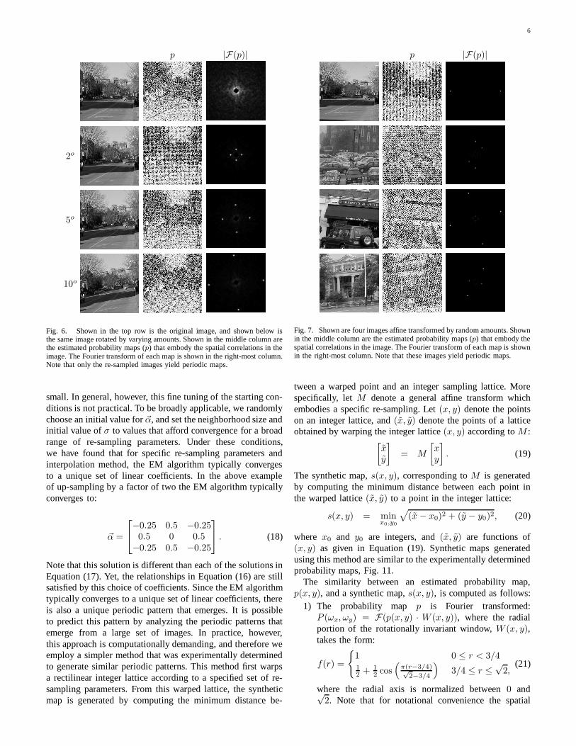
Fig. 6. Shown in the top row is the original image, and shown below isthe same image rotated by varying amounts. Shown in the middle column arethe estimated probability maps (p) that embody the spatial correlations in theimage. The Fourier transform of each map is shown in the right-most column.Note that only the re-sampled images yield periodic maps.

small. In general, however, this fine tuning of the starting con-ditions is not practical. To be broadly applicable, we randomlychoose an initial value for ~α, and set the neighborhood size andinitial value of σ to values that afford convergence for a broadrange of re-sampling parameters. Under these conditions,we have found that for specific re-sampling parameters andinterpolation method, the EM algorithm typically convergesto a unique set of linear coefficients. In the above exampleof up-sampling by a factor of two the EM algorithm typicallyconverges to:

~α =

−0.25 0.5 −0.250.5 0 0.5

−0.25 0.5 −0.25

. (18)

Note that this solution is different than each of the solutions inEquation (17). Yet, the relationships in Equation (16) are stillsatisfied by this choice of coefficients. Since the EM algorithmtypically converges to a unique set of linear coefficients, thereis also a unique periodic pattern that emerges. It is possibleto predict this pattern by analyzing the periodic patterns thatemerge from a large set of images. In practice, however,this approach is computationally demanding, and therefore weemploy a simpler method that was experimentally determinedto generate similar periodic patterns. This method first warpsa rectilinear integer lattice according to a specified set of re-sampling parameters. From this warped lattice, the syntheticmap is generated by computing the minimum distance be-

p |F(p)|

Fig. 7. Shown are four images affine transformed by random amounts. Shownin the middle column are the estimated probability maps (p) that embody thespatial correlations in the image. The Fourier transform of each map is shownin the right-most column. Note that these images yield periodic maps.

tween a warped point and an integer sampling lattice. Morespecifically, let M denote a general affine transform whichembodies a specific re-sampling. Let (x, y) denote the pointson an integer lattice, and (x, y) denote the points of a latticeobtained by warping the integer lattice (x, y) according to M :

[

xy

]

= M

[

xy

]

. (19)

The synthetic map, s(x, y), corresponding to M is generatedby computing the minimum distance between each point inthe warped lattice (x, y) to a point in the integer lattice:

s(x, y) = minx0,y0

√

(x − x0)2 + (y − y0)2, (20)

where x0 and y0 are integers, and (x, y) are functions of(x, y) as given in Equation (19). Synthetic maps generatedusing this method are similar to the experimentally determinedprobability maps, Fig. 11.

The similarity between an estimated probability map,p(x, y), and a synthetic map, s(x, y), is computed as follows:

1) The probability map p is Fourier transformed:P (ωx, ωy) = F(p(x, y) · W (x, y)), where the radialportion of the rotationally invariant window, W (x, y),takes the form:

f(r) =

{

1 0 ≤ r < 3/412 + 1

2 cos(

π(r−3/4)√

2−3/4

)

3/4 ≤ r ≤√

2,(21)

where the radial axis is normalized between 0 and√2. Note that for notational convenience the spatial

7

Fig. 8. Shown are two images that were consecutively re-sampled (top left:upsampled by 15% and then rotated by 5◦; top right : rotated by 5◦ and thenupsampled by 15%). Shown in the second row are the estimated probabilitymaps that embody the spatial correlations in the image. The magnitude ofthe Fourier transform of each map is shown in the bottom column - note themultiple set of peaks that correspond to both the rotation and up-sampling.

arguments on p(·) and P (·) will be dropped.2) The Fourier transformed map P is then high-pass filtered

to remove undesired low frequency noise: PH = P ·H , where the radial portion of the rotationally invarianthighpass filter, H , takes the form:

h(r) =1

2− 1

2cos

(

πr√2

)

, 0 ≤ r ≤√

2. (22)

3) The high-passed spectrum PH is then normalized,gamma corrected in order to enhance frequency peaks,and then rescaled back to its original range:

PG =

(

PH

max(|PH|)

)4

× max(|PH |). (23)

4) The synthetic map s is simply Fourier transformed: S =F(s).

5) The measure of similarity between p and s is then givenby:

M (p, s) =∑

ωx,ωy

|PG(ωx, ωy)| · |S(ωx, ωy)|, (24)

where |·| denotes absolute value (note that this similaritymeasure is phase insensitive).

A set of synthetic probability maps are first generatedfrom a number of different re-sampling parameters. For agiven probability map p, the most similar synthetic map, s? ,is found through a brute-force search over the entire set:s? = arg maxs M (p, s). If the similarity measure, M (p, s?), is

original

forgery

probability map (p)

Fig. 9. Shown are the original image and a forgery. The forgery consistsof splicing in a new license plate number. Shown below is the estimatedprobability map (p) of the forgery, and the magnitude of the Fourier transform(F(p)) of a region in the license plate (left) and on the car trunk (right). Theperiodic pattern (spikes in F(p)) in the license plate suggests that this regionwas re-sampled.

8

original

forgery

probability map (p)

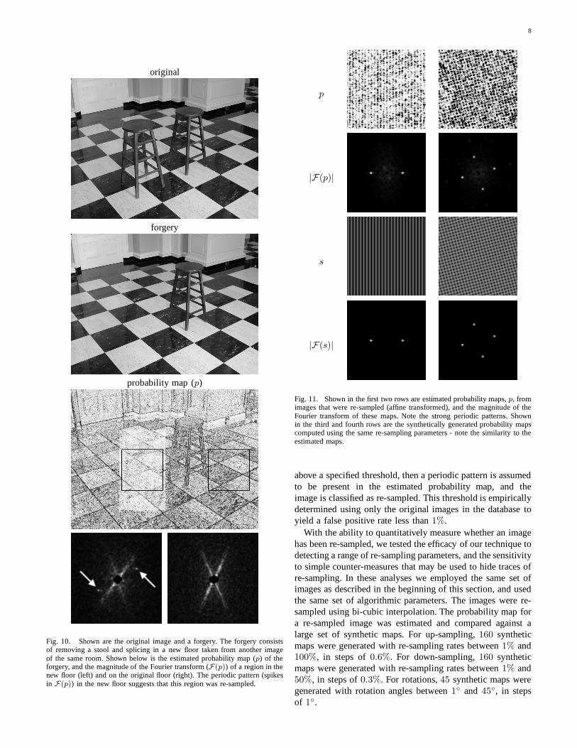
Fig. 10. Shown are the original image and a forgery. The forgery consistsof removing a stool and splicing in a new floor taken from another imageof the same room. Shown below is the estimated probability map (p) of theforgery, and the magnitude of the Fourier transform (F(p)) of a region in thenew floor (left) and on the original floor (right). The periodic pattern (spikesin F(p)) in the new floor suggests that this region was re-sampled.

p

|F(p)|

s

|F(s)|

Fig. 11. Shown in the first two rows are estimated probability maps, p, fromimages that were re-sampled (affine transformed), and the magnitude of theFourier transform of these maps. Note the strong periodic patterns. Shownin the third and fourth rows are the synthetically generated probability mapscomputed using the same re-sampling parameters - note the similarity to theestimated maps.

above a specified threshold, then a periodic pattern is assumedto be present in the estimated probability map, and theimage is classified as re-sampled. This threshold is empiricallydetermined using only the original images in the database toyield a false positive rate less than 1%.

With the ability to quantitatively measure whether an imagehas been re-sampled, we tested the efficacy of our technique todetecting a range of re-sampling parameters, and the sensitivityto simple counter-measures that may be used to hide traces ofre-sampling. In these analyses we employed the same set ofimages as described in the beginning of this section, and usedthe same set of algorithmic parameters. The images were re-sampled using bi-cubic interpolation. The probability map fora re-sampled image was estimated and compared against alarge set of synthetic maps. For up-sampling, 160 syntheticmaps were generated with re-sampling rates between 1% and100%, in steps of 0.6%. For down-sampling, 160 syntheticmaps were generated with re-sampling rates between 1% and50%, in steps of 0.3%. For rotations, 45 synthetic maps weregenerated with rotation angles between 1◦ and 45◦, in stepsof 1◦.

9

1 3 5 10 20 30 40 50 60 70 80 900

50

100

up−sampling (%)

perc

ent c

orre

ct

1 3 5 10 15 20 25 30 35 40 450

50

100

down−sampling (%)

perc

ent c

orre

ct

1 3 5 10 15 20 25 30 35 40 450

50

100

rotation (degrees)

per

cen

t co

rrec

t

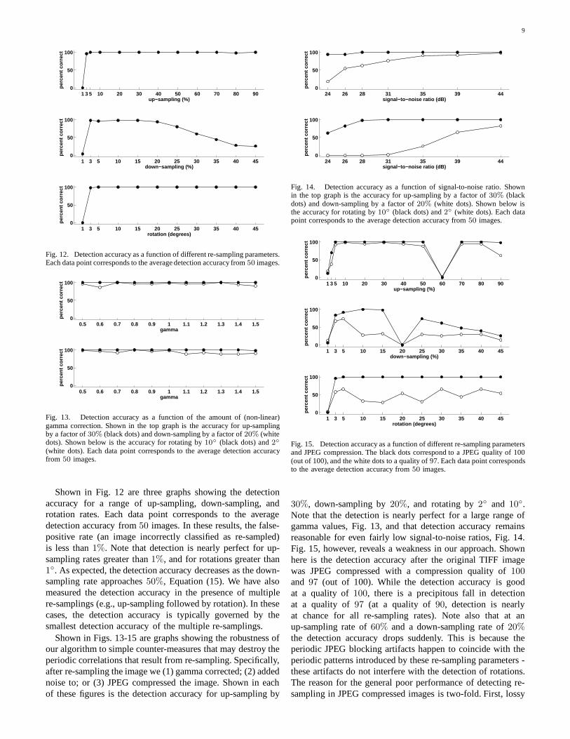
Fig. 12. Detection accuracy as a function of different re-sampling parameters.Each data point corresponds to the average detection accuracy from 50 images.

0.5 0.6 0.7 0.8 0.9 1 1.1 1.2 1.3 1.4 1.50

50

100

gamma

per

cen

t co

rrec

t

0.5 0.6 0.7 0.8 0.9 1 1.1 1.2 1.3 1.4 1.50

50

100

gamma

per

cen

t co

rrec

t

Fig. 13. Detection accuracy as a function of the amount of (non-linear)gamma correction. Shown in the top graph is the accuracy for up-samplingby a factor of 30% (black dots) and down-sampling by a factor of 20% (whitedots). Shown below is the accuracy for rotating by 10◦ (black dots) and 2◦

(white dots). Each data point corresponds to the average detection accuracyfrom 50 images.

Shown in Fig. 12 are three graphs showing the detectionaccuracy for a range of up-sampling, down-sampling, androtation rates. Each data point corresponds to the averagedetection accuracy from 50 images. In these results, the false-positive rate (an image incorrectly classified as re-sampled)is less than 1%. Note that detection is nearly perfect for up-sampling rates greater than 1%, and for rotations greater than1◦. As expected, the detection accuracy decreases as the down-sampling rate approaches 50%, Equation (15). We have alsomeasured the detection accuracy in the presence of multiplere-samplings (e.g., up-sampling followed by rotation). In thesecases, the detection accuracy is typically governed by thesmallest detection accuracy of the multiple re-samplings.

Shown in Figs. 13-15 are graphs showing the robustness ofour algorithm to simple counter-measures that may destroy theperiodic correlations that result from re-sampling. Specifically,after re-sampling the image we (1) gamma corrected; (2) addednoise to; or (3) JPEG compressed the image. Shown in eachof these figures is the detection accuracy for up-sampling by

24 26 28 31 35 39 440

50

100

signal−to−noise ratio (dB)

perc

ent c

orre

ct

24 26 28 31 35 39 440

50

100

signal−to−noise ratio (dB)

perc

ent c

orre

ct

Fig. 14. Detection accuracy as a function of signal-to-noise ratio. Shownin the top graph is the accuracy for up-sampling by a factor of 30% (blackdots) and down-sampling by a factor of 20% (white dots). Shown below isthe accuracy for rotating by 10◦ (black dots) and 2◦ (white dots). Each datapoint corresponds to the average detection accuracy from 50 images.

1 3 5 10 20 30 40 50 60 70 80 900

50

100

up−sampling (%)

perc

ent c

orre

ct

1 3 5 10 15 20 25 30 35 40 450

50

100

down−sampling (%)

perc

ent c

orre

ct

1 3 5 10 15 20 25 30 35 40 450

50

100

rotation (degrees)

per

cen

t co

rrec

t

Fig. 15. Detection accuracy as a function of different re-sampling parametersand JPEG compression. The black dots correspond to a JPEG quality of 100(out of 100), and the white dots to a quality of 97. Each data point correspondsto the average detection accuracy from 50 images.

30%, down-sampling by 20%, and rotating by 2◦ and 10◦.Note that the detection is nearly perfect for a large range ofgamma values, Fig. 13, and that detection accuracy remainsreasonable for even fairly low signal-to-noise ratios, Fig. 14.Fig. 15, however, reveals a weakness in our approach. Shownhere is the detection accuracy after the original TIFF imagewas JPEG compressed with a compression quality of 100and 97 (out of 100). While the detection accuracy is goodat a quality of 100, there is a precipitous fall in detectionat a quality of 97 (at a quality of 90, detection is nearlyat chance for all re-sampling rates). Note also that at anup-sampling rate of 60% and a down-sampling rate of 20%the detection accuracy drops suddenly. This is because theperiodic JPEG blocking artifacts happen to coincide with theperiodic patterns introduced by these re-sampling parameters -these artifacts do not interfere with the detection of rotations.The reason for the general poor performance of detecting re-sampling in JPEG compressed images is two-fold. First, lossy

10

JPEG compression introduces noise into the image (e.g., acompression quality of 90 introduces, on average, 28 db ofnoise), and as can be seen in Fig. 14, this amount of noisesignificantly affects the detection accuracy. Second, the blockartifacts introduced by JPEG introduce very strong periodicpatterns that interfere with and mask the periodic patternsintroduced by re-sampling. In preliminary results, we foundthat under JPEG 2000 compression, detection remains robustdown to 2 bits/pixel, with significant deterioration below 1.5bits/pixel. This improved performance is most likely due to thelack of the blocking artifacts introduced by standard JPEG.

We have also tested our algorithm against GIF formatimages. Specifically, a 24-bit color (RGB) image was sub-jected to a range of re-samplings and then converted to 8-bit indexed color format (GIF). This conversion introducesapproximately 21 db of noise. For rotations greater than 10◦,up-sampling greater than 20%, and down-sampling greaterthan 15%, detection accuracy is, on average, 80%, 60%, and30%, respectively, with a less than 1% false-positive rate.While not as good as the uncompressed TIFF images, thesedetection rates are roughly what would be expected with thelevel of noise introduced by GIF compression, Fig. 14. Andfinally, we have tested our algorithm against RGB imagesreconstructed from a color filter array (CFA) interpolationalgorithm. In this case, the non-linear CFA interpolation doesnot interfere with our ability to detect re-sampling.

In summary, we have shown that for uncompressed TIFFimages, and JPEG and GIF images with minimal compressionwe can detect whether an image region has been re-sampled(scaled, rotated, etc.), as might occur when an image has beentampered with.

IV. DISCUSSION

When creating digital forgeries, it is often necessary toscale, rotate, or distort a portion of an image. This processinvolves re-sampling the original image onto a new lattice.Although this re-sampling process typically leaves behindno perceptual artifacts, it does introduce specific periodiccorrelations between the image pixels. We have shown howand when these patterns are introduced, and described atechnique to automatically find such patterns in any regionof an image. This technique is able to detect a broad range ofre-sampling rates, and is reasonably robust to simple counter-attacks. This technique is not able to uniquely identify thespecific re-sampling amount, as different re-samplings willmanifest themselves with similar periodic patterns. Althoughwe have only described how linear or cubic interpolation canbe detected, there is no inherent reason why more sophisticatednon-linear interpolation techniques (e.g., edge preserving inter-polation) cannot be detected using the same basic frameworkof estimating local spatial correlations.

Our technique works in the complete absence of any digitalwatermark or signature, offering a complementary approachto authenticating digital images. While statistical techniquessuch as that presented here pose many challenges, we believethat their development will be important to contend with thecases when watermarking technologies are not applicable.

The major weakness of our approach is that it is currentlyonly applicable to uncompressed TIFF images, and JPEG andGIF images with minimal compression. We believe, however,that this technique will still prove useful in a number ofdifferent digital forensic settings - for example a court of lawmight insist that digital images be submitted into evidence inan uncompressed high-resolution format.

We are currently exploring several other techniques for de-tecting other forms of digital tampering. We believe that manycomplementary techniques such as that presented here, andthose that we (e.g., [22]) and others develop, will be neededto reliably expose digital forgeries. There is little doubt thateven with the development of a suite of detection techniques,more sophisticated tampering techniques will emerge, whichin turn will lead to the development of more detection tools,and so on, thus making the creation of forgeries increasinglymore difficult.

REFERENCES

[1] S. Katzenbeisser and F. Petitcolas, Information Techniques for Steganog-raphy and Digital Watermarking. Artec House, 2000.

[2] I. Cox, M. Miller, and J. Bloom, Digital Watermarking. MorganKaufmann Publishers, 2002.

[3] G. Friedman, “The trustworthy camera: Restoring credibility to thephotographic image,” IEEE Transactions on Consumer Electronics,vol. 39, no. 4, pp. 905–910, 1993.

[4] M. Schneider and S.-F. Chang, “A robust content-based digital signaturefor image authentication,” in IEEE International Conference on ImageProcessing, vol. 2, 1996, pp. 227–230.

[5] D. Storck, “A new approach to integrity of digital images,” in IFIPConference on Mobile Communication, 1996, pp. 309–316.

[6] B. Macq and J.-J. Quisquater, “Cryptology for digital tv broadcasting,”Proceedings of the IEEE, vol. 83, no. 6, pp. 944–957, 1995.

[7] S. Bhattacharjee and M. Kutter, “Compression-tolerant image authenti-cation,” in IEEE International Conference on Image Processing, vol. 1,1998, pp. 435–439.

[8] C. Honsinger, P.Jones, M.Rabbani, and J. Stoffel, “Lossless recovery ofan original image containing embedded data,” U.S. Patent Application,Docket No. 77102/E-D, 1999.

[9] J. Fridrich, M. Goljan, and M. Du, “Invertible authentication,” in Pro-ceedings of SPIE, Security and Watermarking of Multimedia Contents,2001.

[10] E. Lin, C. Podilchuk, and E. Delp, “Detection of image alterationsusing semi-fragile watermarks,” in Proceedings of SPIE, Security andWatermarking of Multimedia Contents II, vol. 3971, 2000, pp. 52–163.

[11] C. Rey and J.-L. Dugelay, “Blind detection of malicious alterations onstill images using robust watermarks,” in IEE Seminar: Secure Imagesand Image Authentication, 2000, pp. 7/1–7/6.

[12] G.-J. Yu, C.-S. Lu, H.-Y. Liao, and J.-P. Sheu, “Mean quantizationblind watermarking for image authentication,” in IEEE InternationalConference on Image Processing, vol. 3, 2000, pp. 706–709.

[13] C.-Y. Lin and S.-F. Chang, “A robust image authentication algorithmsurviving jpeg lossy compression,” in Proceedings of SPIE, Storage andRetrieval of Image/Video Databases, vol. 3312, 1998, pp. 296–307.

[14] M. Yeung and F. Mintzer, “An invisible watermarking technique forimage verification,” in Proceedings of the International Conference onImage Processing, vol. 1, 1997, pp. 680–683.

[15] D. Kundur and D. Hatzinakos, “Digital watermarking for tell-tale tamperproofing and authentication,” Proceedings of the IEEE, vol. 87, no. 7,pp. 1167–1180, 1999.

[16] M. U. Celik, G. Sharma, E. Saber, and A. M. Tekalp, “Hierarchicalwatermarking for secure image authentication with localization,” IEEETransactions on Image Processing, vol. 11, no. 6, pp. 585–595, 2002.

[17] J. Fridrich, “Security of fragile authentication watermarks with localiza-tion,” in Proceedings of SPIE, Electronic Imaging, vol. 4675, 2002, pp.691–700.

[18] J. Fridrich and M. Goljan, “Images with self-correcting capabilities,” inProceedings of the IEEE International Conference on Image Processing,vol. 3, 1999, pp. 792–796.

11

[19] S. Craver, M. Wu, B. Liu, A. Stubblefield, B. Swartzlander, and D. Wal-lach, “Reading between the lines: Lessons from the SDMI challenge,”in 10th USENIX Security Symposium, Washington DC, 2001.

[20] A. V. Oppenheim and R. W. Schafer, Discrete-Time Signal Processing.Prentice Hall, 1989.

[21] A. Dempster, N. Laird, and D. Rubin, “Maximum lilelihood fromincomplete data via the EM algorithm,” Journal of the Royal StatisticalSociety, vol. 99, no. 1, pp. 1–38, 1977.

[22] H. Farid and S. Lyu, “Higher-order wavelet statistics and their applica-tion to digital forensics,” in IEEE Workshop on Statistical Analysis inComputer Vision, Madison, Wisconsin, 2003.

Appendix A: EM Algorithm

/* Initialize */choose a random ~α0

choose N and σ0

set p0 to the reciprocal of the range of the signal ~yset Y as in Equation (14)set h to be a binomial low-pass filter of size (Nh ×Nh)

n = 0repeat

/* expectation step */for each sample i

R(i) =∣

∣

∣y(i) −∑N

k=−N αn(k)y(i + k)∣

∣

∣/* residual */

endR = R ? h /* spatially average the residual error */for each sample iP (i) = 1

σn

√2π

e−R(i)2/2σ2

n /* conditional probability */

w(i) = P (i)P (i)+p0

/* posterior probability */end

/* maximization step */W = 0for each sample i

W (i, i) = w(i) /* weighting matrix */end

σn+1 =( �

iw(i)R2(i)

�i w(i)

)1/2

/* new variance estimate */

~αn+1 = (Y T WY )−1Y T W~y /* new estimate */n = n + 1

until ( ‖~αn − ~αn−1‖ < ε ) /* stopping condition */

Alin C Popescu received the B.E. degree in Elec-trical Engineering in 1999 from the University Po-litehnica of Bucharest, and the M.S. degree in Com-puter Science in 1999 from Universite de Marne-la-Vallee. He is currently a Ph.D. candidate in Com-puter Science at Dartmouth College.

Hany Farid received the B.S. degree in ComputerScience and Applied Mathematics in 1988 fromthe Unversity of Rochester, and then received thePh.D. degree in 1997 in Computer Science from theUniversity of Pennsylvania. He joined the Dartmouthfaculty in 1999, following a two year post-doctoralposition in Brain and Cognitive Sciences at theMassachusetts Institute of Technology.