extended measurements in pose graph optimization · extended measurements in pose graph...
TRANSCRIPT

Extended Measurementsin Pose Graph Optimization
Master thesis
Irvin Aloise
RoCoCo - Cognitive robot teams laboratory
Department of Computer, Control and Management Engineering Antonio Ruberti
Sapienza University of Rome
Supervisor:
Prof. Dr. Giorgio GrisettiCosupervisor:
Eng. Dominik Schlegel
October 9, 2017


Abstract
The goal of this Master’s Thesis is the design and development of a graph-optimizationsystem tailored for SLAM pipelines. The work focuses on simplicity, accuracy and speed,reaching excellent results in each of the targeted fields.
In particular, this back-end aims attention at 3D pose-graphs and 3D pose-landmarkproblems, producing outcomes comparable to current state-of-the-art systems like g2o
[1].
At its core there is a novel error function for SE(3) objects based on the concept ofmatrices’ chordal distance. This approach reduces the problem’s non-linearity bringingseveral benefits to the computation. The fastness of the system is due to a well-designedimplementation that performs zero memory copy during the iterative part and thatexploits SIMD instructions of modern CPUs and a smart use of the CPU cache.
Finally, the system has been tested on both synthetic and real-world datasets andin both scenarios it succeeded in its purposes, being able to produce results better orcomparable to state-of-the-art systems in only 5 thousands lines of code.
i

Nomenclature
Notation
ARB(α, β, γ) Rotation from frame A to frame B expressed in AAtB(tx, ty, tz) Translation from frame A to frame B expressed in AATB(R, t) Transformation from frame A to B expressed in AAτB(R, t) Transformation from frame A to B expressed in A (vectorized)
btc× Skew-symmetric matrix of a vector t ∈ R3×3
Acronyms and Abbreviations
SLAM Simultaneous localization and mapping
SfM Structure from Motion
BA Bundle Adjustment
SCLAM Simultaneous Calibration Localization and Mapping
MAP Maximum A Posteriori
LS Least Squares
PSD Positive Semi-Definite
PDF Probability Distribution Function
Landmark Salient point in the world (2D or 3D)
Feature Specific structural part of interest in an image (2D)
Tracking Procedure of spatial and temporal re-identification of landmarks
Loop closure Interconnection between landmarks in space
GPS Global Positioning System (generally referring to whole unit)
LiDAR Light Detection and Ranging o Laser Imaging Detection and Ranging
Sonar SOund Navigation And Ranging
FLOP Floating Point OPeration
FLOPS Floating Point Operations Per Second
OpenCV Open source Computer Vision (library), www.opencv.org
Git Git revision control, www.git-scm.com
ii

iii

Contents
Abstract i
Nomenclature ii
1 Introduction 1
2 Related Work 3
2.1 Dense Approaches . . . . . . . . . . . . . . . . . . . . . . . . . . . . . . 4
2.2 Olson’s Gradient Descent . . . . . . . . . . . . . . . . . . . . . . . . . . 5
2.3 Smoothing and Mapping . . . . . . . . . . . . . . . . . . . . . . . . . . . 5
2.4 TORO . . . . . . . . . . . . . . . . . . . . . . . . . . . . . . . . . . . . . 6
2.5 G2O . . . . . . . . . . . . . . . . . . . . . . . . . . . . . . . . . . . . . . 6
2.6 GT-SAM . . . . . . . . . . . . . . . . . . . . . . . . . . . . . . . . . . . 6
2.7 HOG-Man . . . . . . . . . . . . . . . . . . . . . . . . . . . . . . . . . . . 7
2.8 Tectonic-SAM . . . . . . . . . . . . . . . . . . . . . . . . . . . . . . . . . 8
2.9 Condensed Measurements . . . . . . . . . . . . . . . . . . . . . . . . . . 8
3 Basics 9
3.1 Least Square SLAM . . . . . . . . . . . . . . . . . . . . . . . . . . . . . 9
3.1.1 Direct Minimization . . . . . . . . . . . . . . . . . . . . . . . . . 11
3.2 Manifolds . . . . . . . . . . . . . . . . . . . . . . . . . . . . . . . . . . . 14
3.3 Sparse Least Squares . . . . . . . . . . . . . . . . . . . . . . . . . . . . . 17
3.4 Factor Graphs . . . . . . . . . . . . . . . . . . . . . . . . . . . . . . . . . 20
4 Typical Problems 22
4.1 Pose Graphs . . . . . . . . . . . . . . . . . . . . . . . . . . . . . . . . . . 22
4.2 Pose-Landmark Graphs . . . . . . . . . . . . . . . . . . . . . . . . . . . 24
4.3 Pose and Landmark Estimation . . . . . . . . . . . . . . . . . . . . . . . 25
4.3.1 Pose-Pose Constraints . . . . . . . . . . . . . . . . . . . . . . . . 26
4.3.2 Pose-Point Constraints . . . . . . . . . . . . . . . . . . . . . . . . 26
iv

Contents v
4.4 Bundle Adjustment . . . . . . . . . . . . . . . . . . . . . . . . . . . . . . 27
4.5 Simultaneous Calibration Localization and Mapping . . . . . . . . . . . 27
5 Solving Factor Graphs with SE3 Variables 30
5.1 Exploit Sparsity . . . . . . . . . . . . . . . . . . . . . . . . . . . . . . . 30
5.1.1 Storage Methods for Sparse Matrices . . . . . . . . . . . . . . . . 32
5.1.2 Cholesky Decomposition . . . . . . . . . . . . . . . . . . . . . . . 33
5.2 Manifold Representation . . . . . . . . . . . . . . . . . . . . . . . . . . . 34
5.2.1 3D Pose-Graph . . . . . . . . . . . . . . . . . . . . . . . . . . . . 34
5.2.2 3D Pose-Landmark . . . . . . . . . . . . . . . . . . . . . . . . . . 36
5.3 Dealing with SE3 Objects . . . . . . . . . . . . . . . . . . . . . . . . . . 38
5.3.1 Chordal Distance Based Error Function . . . . . . . . . . . . . . 38
5.3.2 Benefits in the Re-linearization . . . . . . . . . . . . . . . . . . . 42
5.4 Convergence Results . . . . . . . . . . . . . . . . . . . . . . . . . . . . . 44
6 Software Implementation of the Optimizer 50
6.1 Graph . . . . . . . . . . . . . . . . . . . . . . . . . . . . . . . . . . . . . 51
6.2 The Optimizer . . . . . . . . . . . . . . . . . . . . . . . . . . . . . . . . 51
6.2.1 Linearization and Hessian Composition . . . . . . . . . . . . . . 52
6.2.2 Sparse Linear Solver . . . . . . . . . . . . . . . . . . . . . . . . . 52
6.2.3 Graph Update . . . . . . . . . . . . . . . . . . . . . . . . . . . . 53
6.3 Bottlenecks . . . . . . . . . . . . . . . . . . . . . . . . . . . . . . . . . . 53
6.3.1 Memory management . . . . . . . . . . . . . . . . . . . . . . . . 53
6.3.2 Hessian blocks computation . . . . . . . . . . . . . . . . . . . . . 54
6.4 Performance Results . . . . . . . . . . . . . . . . . . . . . . . . . . . . . 54
7 Use Cases 58
7.1 ProSLAM . . . . . . . . . . . . . . . . . . . . . . . . . . . . . . . . . . . 58
7.2 ProSLAM stud . . . . . . . . . . . . . . . . . . . . . . . . . . . . . . . . 59
7.3 KITTI Dataset . . . . . . . . . . . . . . . . . . . . . . . . . . . . . . . . 59
8 Conclusions 62
8.1 Applications . . . . . . . . . . . . . . . . . . . . . . . . . . . . . . . . . . 62
8.2 Future Works . . . . . . . . . . . . . . . . . . . . . . . . . . . . . . . . . 63
8.2.1 Expand the Addressed Problems . . . . . . . . . . . . . . . . . . 63

Contents vi
8.2.2 Hierarchical Approach . . . . . . . . . . . . . . . . . . . . . . . . 63
Bibliography 64
List of Figures
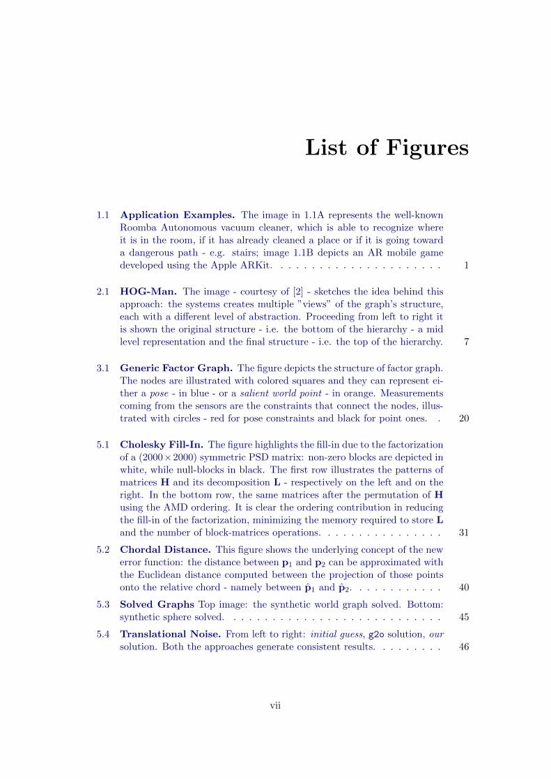
1.1 Application Examples. The image in 1.1A represents the well-knownRoomba Autonomous vacuum cleaner, which is able to recognize whereit is in the room, if it has already cleaned a place or if it is going towarda dangerous path - e.g. stairs; image 1.1B depicts an AR mobile gamedeveloped using the Apple ARKit. . . . . . . . . . . . . . . . . . . . . . 1
2.1 HOG-Man. The image - courtesy of [2] - sketches the idea behind thisapproach: the systems creates multiple ”views” of the graph’s structure,each with a different level of abstraction. Proceeding from left to right itis shown the original structure - i.e. the bottom of the hierarchy - a midlevel representation and the final structure - i.e. the top of the hierarchy. 7
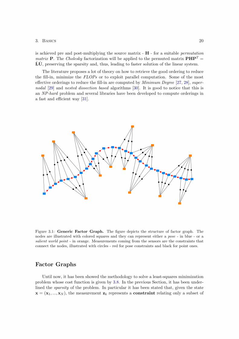
3.1 Generic Factor Graph. The figure depicts the structure of factor graph.The nodes are illustrated with colored squares and they can represent ei-ther a pose - in blue - or a salient world point - in orange. Measurementscoming from the sensors are the constraints that connect the nodes, illus-trated with circles - red for pose constraints and black for point ones. . 20
5.1 Cholesky Fill-In. The figure highlights the fill-in due to the factorizationof a (2000×2000) symmetric PSD matrix: non-zero blocks are depicted inwhite, while null-blocks in black. The first row illustrates the patterns ofmatrices H and its decomposition L - respectively on the left and on theright. In the bottom row, the same matrices after the permutation of Husing the AMD ordering. It is clear the ordering contribution in reducingthe fill-in of the factorization, minimizing the memory required to store Land the number of block-matrices operations. . . . . . . . . . . . . . . . 31
5.2 Chordal Distance. This figure shows the underlying concept of the newerror function: the distance between p1 and p2 can be approximated withthe Euclidean distance computed between the projection of those pointsonto the relative chord - namely between p1 and p2. . . . . . . . . . . . 40
5.3 Solved Graphs Top image: the synthetic world graph solved. Bottom:synthetic sphere solved. . . . . . . . . . . . . . . . . . . . . . . . . . . . 45
5.4 Translational Noise. From left to right: initial guess, g2o solution, oursolution. Both the approaches generate consistent results. . . . . . . . . 46
vii

LIST OF FIGURES viii
5.5 Rotational Noise. Figure (A) from left to right: initial guess, g2o
solution, our solution. Figure (B) shows the chi2 of both approachesat each iteration: it is clear the convergence gap between g2o - in blue- and our approach - in orange. The y axis’ scale is logarithmic. Theiterations performed are 10, therefore, the point x = 1 indicates the chi2
of the initial guess. . . . . . . . . . . . . . . . . . . . . . . . . . . . . . . 46
5.6 Advanced Rotational Noise. Figure (A) from left to right: initialguess, g2o solution, our solution. Figure (B) shows the chi2 of bothapproaches at each iteration. g2o’s trend might indicate that the systemgot stuck in a local minimum. . . . . . . . . . . . . . . . . . . . . . . . . 47
5.7 Sphere 6 DoF Noise. Figure (A) from left to right: initial guess, g2osolution, our solution. Figure (B) shows the chi2 of both approaches ateach iteration. From the plot it is clear that g2o converges to a localminimum distant from the optimum. Here our approach instead is ableto converge to the proper solution in less than 40 iterations. . . . . . . . 48
5.8 Advanced Rotational Noise. Figure (A) from left to right: initialguess, g2o solution, our solution. Figure (B) shows the chi2 of bothapproaches at each iteration. Even if both systems fail in reaching theoptimum, our system is able to generate a fair solution that can be furtherrefined to reach the proper convergence. . . . . . . . . . . . . . . . . . . 48
5.9 Conditioning Methods. The outcomes of the three conditioning meth-ods used to compute the measurements’ information matrix. Given theinitial guess relative to Figure 5.7A, from left to right are illustrated: soft,mid and hard conditioning. . . . . . . . . . . . . . . . . . . . . . . . . . 49
6.1 Pose Graph Optimization Step Time Comparison. Comparisonbetween g2o - in blue - and our system - in orange - of the time requiredto execute an optimization step. Despite the minimalistic implementation,our approach is significantly faster than g2o; the gap increases with thenumber of edges, indicating a slightly better scalability of the proposedsystem with respect to g2o. . . . . . . . . . . . . . . . . . . . . . . . . . 55
6.2 BA Optimization Step Time Comparison. Comparison between g2o
- in blue - and our system - in orange - of the time required to execute anoptimization step. In this case g2o leads always the comparison. . . . . 56
7.1 KIT AnnieWAY acquisition method. The KITTI dataset is acquiredusing an autonomous driving car, equipped with several sensor: a stereo-rig of high resolution cameras, Velodyne 3D laser scanner and a localiza-tion unit based on GPS/GLONASS/IMU. . . . . . . . . . . . . . . . . . 59
LIST OF FIGURES ix
7.2 ProSLAM results. Starting from the top image it is proposed a com-parison between the estimated and the real camera trajectory of sequence00 - respectively in blue and in red. Proceeding from left to right it isproposed the estimation with no map optimization, using g2o and usingour approach as optimizer. In the bottom image it is shown the samecomparison but using sequence 06. . . . . . . . . . . . . . . . . . . . . . 60
7.3 ProSLAM stud results. The top image proposes the estimated andreal camera trajectory of sequence 00 - respectively in blue and in red.Again it is proposed the comparison between open-loop estimation, g2oand our approach. In the bottom image it is shown the same comparisonbut using sequence 06. . . . . . . . . . . . . . . . . . . . . . . . . . . . . 61

List of Tables
6.1 Pose Graph Optimization Total Time Comparison. In this tableare reported the total optimization time required by the two systems tocomplete 10 iterations. The reader might notice that in graphs with moreedges, our approach performs better than g2o. . . . . . . . . . . . . . . 56
6.2 BA Optimization Total Time Comparison. In this table are reportedthe total optimization time required by the two systems to complete 10iterations. The reader might notice an inverted trend with respect to purepose-graph optimization, with our system struggling when the number ofedges increases. . . . . . . . . . . . . . . . . . . . . . . . . . . . . . . . . 57
7.1 ProSLAM Trajectory Error. In this Table are reported the transla-tion and rotation error of the final trajectory on both sequences. Thecontribution of a map optimizer is undeniable, however, the reader mightappreciate the results obtained with our minimalistic approach, which arenot far from the one obtained using the state-of-the-art system g2o. . . 60
7.2 ProSLAM stud Trajectory Error. In this Table are reported thetranslation and rotation error of the final trajectory on both sequences.Even in this case, our approach delivers consistent results. . . . . . . . . 61
x

Chapter 1
Introduction
Mobile robots, in order to accomplish tasks in real world more easily and in anefficient way, need to have a map of the environment and to localize themselves into themap. Furthermore, in some environment it is not possible to rely on external referencesystems - e.g. GPS - and, thus, they can count only on on-board sensors. SimultaneousLocalization and Mapping (SLAM) addresses the problem of learning the map underpose uncertainty.
There are many scenarios in which SLAM is fundamental for the accomplishmentof a task, not only in pure Robotics. SLAM, in fact, is a common problem in differentdomains of application. For example, in Robotics it is fundamental for indoor navigationof mobile robots - e.g. an autonomous vacuum cleaner or a service robot in a museum - orto navigate through extreme environments - e.g. underwater rescues or space exploration.Additionally, new technologies that involve different kind of agents - i.e. not robots - arenow using SLAM. One of the most trending is Augmented Reality (AR). Always morepowerful mobile devices - like smartphones or tablets - are now able to exploit SLAMto deliver stunning virtual experiences. Without any doubts, this technology is going togain always more popularity and to impact on the research in this topic.
(A) (B)
Figure 1.1: Application Examples. The image in 1.1A represents the well-known RoombaAutonomous vacuum cleaner, which is able to recognize where it is in the room, if it has alreadycleaned a place or if it is going toward a dangerous path - e.g. stairs; image 1.1B depicts an ARmobile game developed using the Apple ARKit.
As the reader might notice, SLAM is a popular problem and the research communityis focusing on it since many years. Several solutions have been proposed through theyears and now current state-of-the-art SLAM systems are able to deliver impressiveresults in real-world scenarios. The most used formulation for the SLAM problem is
1

1. Introduction 2
the so-called graph-based SLAM. In this approach, two sub-systems cooperate with eachother to retrieve the best robot trajectory and world configuration given the on-boardsensors’ measurements. Therefore, the full slam system is composed by:
1. Front-end : it exploits sensor data to build an hyper-graph whose nodes are eitherrobot poses or the position of salient points in the world;
2. Back-end : it is in charge of performing non-linear optimization of the graph toretrieve the most likely configuration that suits the measurements.
In this work, we propose a back-end system built from scratch that is able to per-form fast and accurate graph optimization for 3D environments. The work is focused onsimplicity and minimalism also in its implementation, in order to be comprehensible bynon-expert people that want to understand how the system works. Despite its minimal-istic fashion, system’s results are comparable - or even better in some scenarios - to theones of other state-of-the-art systems, thanks to the use of some novel theoretic ideasand to a well-designed implementation. In particular, this work shows the effectivenessof a new error function for SE(3) objects (Section 5.3) and an implementation withzero memory copy during the optimization process (Section 6.3).
The remaining of this document is organized as follows:
• Chapter 2: overview of the problem and of methodologies employed through theyears, with a particular focus on noteworthy systems;
• Chapter 3: problem statement and fundamental theoretic concepts related to thenon-linear optimization problem;
• Chapter 4: sketch of the most common SLAM problem formulations;
• Chapter 5: deeper examination of 3D formulations and further analysis of theproposed approach;
• Chapter 6: details about code design and implementation choices;
• Chapter 7: focus on two full SLAM systems that uses the proposed system ason-line back-end;
• Chapter 8: final considerations and possible future investigations.
Chapter 2
Related Work
Simultaneous Localization and Mapping represents a well known complex mathe-matical problem, based on non-linear optimization. It has been studied by the scientificcommunity since the 80s [3, 4]; during this early stage, its statistical formulation has beeninvestigated, proposing interesting results that will constitute, basically, the baseline forall the future SLAM systems.
After some years, in the 90s, the community came-up with early solutions for theSLAM problem. The first systems able to produce appreciable results in terms of speedand accuracy were based on Extended Kalman Filters (EKF) [5, 6]. EKFs allow to dealwith problem’s non-linearity through effective approximations and to represent multi-variate distributions with a small number of parameters. This success encouraged theresearch community to perform deeper investigations in filtering approaches [7]. Particlefilters started to gain popularity, in particular Rao-Blackwellized Particle Filters [8]: thework of Montemerlo et al. [9] was the first SLAM system able to deal with thousand oflandmarks with a good accuracy.
However, filtering approaches revealed not to be the best answer to the SLAM prob-lem due to the computational complexity of the solution, especially when dimensionsstart to grow. Moreover, system’s accuracy is affected by the problem’s non-linearities,leading to sub-optimal solutions. For these reasons, Maximum A Posteriori (MAP) ap-proaches started to be taken in consideration and the community took a step back to thework of Lu et al. [10]. Filtering-based approaches align local pose frames incrementallyand, thus, different parts of the model are updated independently, generating incon-sistencies in the final model. MAP optimization takes into consideration all the localframes and the relations between them at once, leading to a more consistent model andbetter accuracy. Lu et al. embedded all the pose relations into a network with nodesand edges, allowing efficient optimization. However, when they published their work,the computers’ computational power was not sufficient to deliver good performance and,thus, this solution was put aside.
Nevertheless, this work represents the precursor to one the most intuitive SLAM for-mulation, called graph-based SLAM, that exploits the computing power of recent robotsto deliver impressive performances. In this paradigm, the robot builds an hyper-graphwhose nodes represent either robot poses or salient points in the world - called landmarks- while the hyper-edges encode sensors’ measurements between subsets of nodes.
Graph-based SLAM systems have two main components: front-end and back-end.
3

2. Related Work 4
The former uses data acquired by robot’s sensors to populate the hyper-graph, abstract-ing raw data into a model that is amenable for optimization. The front-end has todetermine the most likely constraint that involves a subset of nodes given an incomingmeasurement, solving the so-called data association problem - short-term and long-term.Short-term data association has to match corresponding features among consecutivesensor measurements - e.g. stating that visual features detected in multiple consecutiveframes represent the same 3D world point. Long-term data association, instead, expressesa more complex problem: it has to associate new measurements to already encounteredworld points, generating the so-called loop-closures - e.g. when a robot passes multipletimes across the same place, it has to recognize that it is re-observing the same pointsin order to generate a map that is consistent with the environment. As for the sensorsused, state-of-the-art systems usually acquire data from cameras (RGB or RDB-D) or3D-LiDARs. The former, in particular, it is gaining much attention from the researchcommunity since they are - generally - cheap and can be mounted basically on everyelectronic device in single or stereo configuration.
This work, however, focuses on system’s back-end, assuming that the given front-endprovides consistent estimates. The back-end takes as input the graph and computes themost-likely map given all the constraints. Systems based on this formulation representthe gold standard for map optimization, thus, in the next sections it is proposed a briefoverview of the most successful implementations.
Dense Approaches
The work of Lu et al. [10] was the first of its kind: map estimation is obtained throughglobal optimization of the error function deriving from constraints between differentposes. They employed a combination of relation-based and location-based representations,where the former were fixed while the latter were treated as free variables. Those pose-relations were used to construct a network whose nodes were robot poses taken fromits trajectory while the constraints between nodes were the pose-relations. Finally, theoptimization problem exploits the network to obtain an objective function that will beminimized: the total energy will decrease as the difference between estimated relativepose that involves two nodes and the measured value tends to zero.
It is good to notice that, in this formulation, the computational power needed for theoptimization grows cubically with the number of variables involved, thus, it is O(N3)where N represents the number of poses. Gutmann and Konolige addressed this problemin their work [11] proposing a method to incrementally build the network and thatdetermines topologically correct relations between poses.
Those approaches opened the path to a series of study in this direction, that will leadto current state-of-the-art optimizers.

2. Related Work 5
Olson’s Gradient Descent
Evident limitations of the previously seen approaches are that their solution highlydepends from the initial estimate of the state. The initial guess is derived from dead-reckoning and, thus, if this is not consistent the system will converge to a local minimum,giving a sub-optimal solution. Olson et al. [12] addressed this issue, proposing a non-linear optimization algorithm that quickly converges to a good approximation of theglobal minimum.
They achieved such results combining two new aspects: the first one is the use of avariant of Stochastic Gradient Descent algorithm, which is robust against local minimaand has a fast convergence rate; the second one is an alternative state-space representationthat has good stability and computational properties. This last feature, in particular,allows to update many poses with a relatively small computational cost in a single iter-ation. Moreover, the memory consumption has been lowered together with the run time- respectively O(N + M) and O(log(N)), where N represents the number of poses andM the number of constraints.
Smoothing and Mapping
Smoothing and Mapping, shortened as SAM, follows the path of global trajectoryoptimization described in the previous Section. Dellaert et al. proposed with square rootSAM (
√SAM) [13] a system able to deal with full SLAM problems: those require the
estimation of the entire set of sensor poses along with the parameters of all the features inthe environment. This problem is also known in Photogrammetry as bundle adjustmentand as structure from motion in Computer Vision.√SAM performs fast optimization exploiting the problem’s intrinsic sparsity. Know-
ing that the measurement Jacobian matrix A is sparse, it is possible to solve the relativelinear system in a faster way through a good variable reordering together with QR orCholesky factorization. For those reasons,
√SAM can optimize larger graph without
losses in terms of performances or accuracy.
Further improvements were introduced with iSAM - incremental SAM - developedby Kaess et al. [14]. The foundations were the same as
√SAM , but in this case
the system operates incrementally, without the need of fully refactoring the whole QR-decomposition, but updating it every time a new measurement is available. With thissolution, it was possible to address real-time problems since the optimization process isfaster than before.
The next iteration of this branch of solutions, is represented by iSAM2 [15]. In thiscase, a new data-structure is proposed, the Bayes tree, to map better the square rootinformation matrix of the problem. Employing Bayes trees, the algorithm is able tofurther improve the performances, exploiting incremental variable re-ordering and fluidrelinearization, eliminating the need for periodic batch steps.

2. Related Work 6
TORO
Grisetti et al. proposed in their work TORO [16] - Tree-based netwORk Optimizer- an extension of Olson’s algorithm to efficiently manage 2D and 3D graph-based opti-mization problems.
This frameworks has several features that allow it to achieve good performances interms of speed and accuracy. The first one is a revisited version of the standard StochasticGradient Descent used to perform the optimization process, together with a techniqueto efficiently distribute the rotational error over a sequence of 3D poses [17]. In fact, dueto the non-commutativity of rotational angles in 3D, major problems may arise whenapplying approaches that are designed for a 2D world. As a result, TORO converges byorders of magnitude faster with respect to previous approaches.
Moreover, it employs a tree parametrization of the nodes [18] that significantly im-proves the performances and allows to deal with arbitrary network topologies. Thisconsented the authors to bound algorithm complexity to the size of the mapped areaand not to the trajectory’s length, yielding accurate maps of the environment in a smallamount of time.
G2O
The work of Kummerle et al. [1] is an open-source C++ frameworks for optimizingnon-linear least squares problems that can be represented as a graph. Its generalitytogether with a cross-platform implementation made g2o one of the most successfulgraph optimization tool, which is employed in many state-of-the-art full SLAM systems.
This work focuses on efficiency, which is achieved at various levels: it exploits graphsparsity and takes advantage of the graph’s special structure to perform fast optimization;it uses advanced methods - Cholesky decomposition through CHOLMOD library - tosolve sparse linear system; finally, it utilizes modern processor’s features to performfast math operation optimizing cache usage - e.g. SIMD instructions. Moreover, thisframeworks offers the possibility to choose between different algorithms - i.e. Gauss-Newton, Levenberg-Marquardt - and linear solvers - direct and iterative.
Our approach still delivers comparable performances with respect to g2o while beinglightweight and more simple to include in a full SLAM pipeline. In fact, g2o is a bigframework, with over 40 thousands lines of code and, thus, its inclusion may add weightto the system.
GT-SAM
GT-SAM is a C++ library developed by Dellaert et al. [19] at the Georgia Instituteof Technology, which provides solution to a wide range of SLAM and Structure From

2. Related Work 7
Motion (SfM) problems, based on factor-graph optimization. It provides both C++ andMATLAB implementations that allow to easily develop and visualize problem solutions.
This work - like it has been previously seen in g2o - also focuses on efficient optimiza-tion and takes advantage of the graph sparsity to deliver fast and accurate performances.However, this framework is even more big and complex - over 300 thousands lines of code- making it very difficult to unravel and understand what is under the hood.
HOG-Man
Grisetti et al. in their work [2] proposed an optimization system designed for accurate,fast and memory efficient on-line operations: HOG-Man - which stands for HierarchicalOptimization on Manifolds.
Figure 2.1: HOG-Man. The image - courtesy of [2] - sketches the idea behind this approach:the systems creates multiple ”views” of the graph’s structure, each with a different level ofabstraction. Proceeding from left to right it is shown the original structure - i.e. the bottom ofthe hierarchy - a mid level representation and the final structure - i.e. the top of the hierarchy.
At its core there is a hierarchical approach to graph optimization: during on-linemapping, it optimizes only the coarse structure of the environment and not the wholemap. The simplified problem that is solved, however, contains all the relevant informationto let the front-end solve properly the data association problem.
It is good to notice, that there are different level of abstractions: the bottom is theoriginal input, while higher levels are always more compact. When the top levels aremodified, only portions of the underlying ones are updated, namely the ones subjectto consistent modifications. This method limits the computational power needed foron-line operations while preserving global consistency, outperforming several previousapproaches.

2. Related Work 8
Tectonic-SAM
Ni et al. propose a way to reduce the computational effort due to the linearizationupdate, based on sub-map partitioning: Tectonic SAM [20] - shortened as T-SAM.
The original problem is addressed through a divide and conquer approach whichproduces local sub-maps. Those smaller maps are individually optimized and then thelocal linearization can be cached and reused when sub-maps are combined into a globalmap, speeding up the linearization process. Sub-maps have a base node that capturetheir global position and the authors showed that, under mild assumptions, this approachleads to the exact solution.
The next iteration - called T-SAM2 [21] - proposes an algorithm that partitions theSLAM factor-graph into a sub-map tree, performing the optimization from leaves to root.In T-SAM, partitioning was done using edge separators; moreover, T-SAM was not ableto maintain hierarchical maps, leading to poor scalability with respect to larger datasets.All those problems were addressed in T-SAM2, where partitioning is done employing thenested dissection algorithm that, together with a novel multi-level approach, provides amore efficient and robust exact solution.
Condensed Measurements
The solution of least-squares problems that can be represented as factor-graph -like in SLAM and SfM - is contingent to both initial estimate and sensor models’ non-linearities. Grisetti et al. proposed a way to enlarge the convergence basin based on thedivide and conquer approach that exploits the factor-graph’s structure [22].
The core of this formulation is to divide the graph into small locally connected sub-graph, each of which represents a sub-problem that can be robustly solved - like it hasbeen suggested in previous systems like HOG-Man [2] and T-SAM [21]. In order toconsistently combine the local sub-graphs, the authors build a simple factor-graph fromthe sub-graphs, constraining the relative positions of the variables in the solution. Forthis reason, the sub-graphs are called condensed measurements. The resulting problemis more convex with respect to the original one and, thus, there are more chances offinding the correct minimum that can be used as initial guess for standard minimizationalgorithms - e.g. Levenberg-Marquardt.
This formulation allows to recover from bad initial estimations, where most of theother approaches fail - both batch and direct ones - but, unfortunately, it does not deliverreal-time performances.

Chapter 3
Basics
The goal of this chapter is to introduce the reader to the mathematical fundamentalsunderlying the system developed. Obviously, it will be a brief overview, therefore, ref-erences to literature are provided if the reader would like to go more in detail with theproposed concepts.
Least Square SLAM
In this section it proposed an insight of least-squares state estimation of non-linearstationary systems [23].
Suppose to have a stationary system W whose state is parametrized by a set of Nnon-observable state variables x = x1, ...,xN. Suppose that it is possible to indirectlyobserve the system state with different generic sensors, those will generate a set of Kmeasurements represented by z = z1, ..., zK, where zk is intended to be the kth
measurement. Since the measurements are affected by noise, those are assumed to berandom variables. Moreover, the state embeds all the knowledge needed to predictthe measurements’ distribution.
Since measurements are affected by noise, it is impossible to compute the state giventhe measurements. What is possible to evaluate, instead, is the states’ distribution knownthe measurements, which can be formalized as following conditional probability :
p (x|z) = p (x1, ...,xN |z1, ..., zK) =
= p (x1:N |z1:K) (3.1)
The probability distribution 3.1 is complex to retrieve in close form, for several rea-sons:
• The mapping between measurements and states can be highly non-linear, producinga multi-modal probability distribution with a complex shape.
• Each measurement zk in general observes only a subset of the state parameters.Moreover, the number of measurements may not be sufficient to fully characterizethe state distribution.
9

3. Basics 10
• Measurements can be wrong - generating outliers - or it is impossible to map anyof the state variable to a specified measurement.
However, what is possible to compute more easily is an estimate of the probability3.1. To do so, we analyze the conditional distribution p (zk|x): this is a predictivedistribution called sensor model or observation model, which formalizes the probabilityof having a certain measurement assuming to know system’s state. Extending this to allthe measurements, you will get the following distribution:
p (z|x) = p (z1:K |x1:N ) (3.2)
As it has been stated before, the state fully describes the measurements, renderingthe single distributions p (zk|x) independent from each other. Exploiting this feature, itis possible to rewrite the 3.2 as follows:
p (z1:K |x1:N ) =K∏k=1
p (zk|x1:N ) (3.3)
The equation 3.3 describes the measurements’ likelihood given the state. Recallingthe Bayes rule [24] and applying it to 3.1 you will obtain the following relation:
p (x1:N |z1:K) =
likelihood
p (z1:K |x1:N )
prior
p (x1:N )
p (z1:K)
normalizer
=
=
∏Kk=1 p (zk|x1:N ) px
pz=
= ηzpx
K∏k=1
p (zk|x1:N )
In this relation, p (x1:N ) represents our prior knowledge about the state distributionand, thus, supposing to know nothing about it, it is represented by a uniform distribu-tion whose value is a constant px. p (z1:K) instead is just a normalizer for the overallprobability function and does not depend from the states, therefore it is assumed to bea constant pz. This leads to the following relation:
p (x1:N |z1:K) ∝K∏k=1
p (zk|x1:N ) (3.4)
Equation 3.4 represents the core of the entire least-square formulation. This will beexploited in the next subsections to approximate the distribution of interest, minimizinga defined cost function.

3. Basics 11
Direct Minimization
Starting from the relation 3.4 it is possible to initialize a minimization problem.Assuming that the measurement are affected by Additive White Gaussian Noise, theobservation model probability p (zk|x1:N ) will be described by a Gaussian distributionN (µ,Ω−1), leading to the equation
p (zk|x1:N ) ∝ exp (−(zk − zk)Ωk(zk − zk)) (3.5)
where zk is the prediction of the measurement given the state, while Ωk = Σ−1k repre-
sents conditional measurement’s information matrix. The predicted measurement zk isa function of the state; in particular it is obtained applying the sensor model hk(·) tothe state, in formulæ:
zk = hk(x) (3.6)
In SLAM - and other similar problems like SfM - the sensor model is a highly non-linearfunction, making the problem more complex and heavy from a computational point ofview. Nevertheless, generally the sensor model is smooth enough to be approximatedwith its first-order Taylor expansion in the neighbor of a linearization point x, leadingto:
hk(x + ∆x) ≈ hk(x) +∂hk(x)
∂x
∣∣∣∣x=x
∆x = hk(x) + Jk∆x (3.7)
where Jk = ∂hk(x)∂x
∣∣∣∣x=x
is the Jacobian evaluated in x = x.
The next step consists in finding a linearization point x? that maximizes the obser-vation model, leading to the following relations:
x? = argmaxx
p(z|x) =
= argmaxx
K∏k=1
p(zk|x) =
= argmaxx
K∏k=1
exp(−(hk(x)− zk)
TΩk(hk(x)− zk))
=
= argminx
K∑k=1
((hk(x)− zk)
TΩk(hk(x)− zk))
The relation ek(x) = hk(x) − zk represents the error function, and, thus, the optimallinearization point will be given by the minimization of the following cost function:

3. Basics 12
F (x) =K∑k=1
eTk (x)Ωkek(x)
ek(x)
(3.8)
In order to find the optimum linearization point, the system must start from a reasonableinitial guess x - to avoid local minima - and apply an increment ∆x directed toward x?.Applying the perturbation ∆x in the error function and approximating again throughthe first-order Taylor expansion we will obtain
ek(x + ∆x) =(hk(x + ∆x)− zk)
TΩk(hk(x + ∆x)− zk))
=
≈ (Jk∆x + hk(x)− zk)TΩk(Jk∆x + hk(x)− zk) =
= (Jk∆x + ek(x))TΩk(Jk∆x + ek(x)) (3.9)
Further expanding the quantities in the equation 3.9, it is possible to obtain the followingrelation:
ek(x + ∆x) ≈ ∆xTHk
JTk ΩkJk ∆x + 2
bk
JTk Ωkek(x) ∆x +
ck
eTk (x)Ωkek(x) =
= ∆xTHk∆x + 2 bk∆x + ck (3.10)
Extending the perturbation to the total cost function expressed in equation 3.8 andplugging what stated in 3.10 we will obtain:
F (x + ∆x) ≈K∑k=1
[∆xTHk∆x + 2 bk∆x + ck
]=
= ∆xT
[K∑k=1
Hk
]H
∆x + 2
[K∑k=1
bk
]b
∆x +K∑k=1
ck
c
=
= ∆xTH∆x + 2 b∆x + c (3.11)
It is good to notice that equation 3.11 represents a quadratic form in ∆x. Thus,finding the minimum of this formula will give us the optimal perturbation ∆x such that
x? = x + ∆x
In order to find the minimum of equation 3.11 we derive it in ∆x, we equal the derivativeto zero and finally we solve the resulting equation for ∆x; in formulæ:

3. Basics 13
∂(∆xTH∆x + 2 b∆x + c
)∂∆x
= 2 H∆x + 2 b = 0 (3.12)
Therefore, in order to find the solution of equation 3.12 and finally get to the optimalperturbation, we must solve the following linear system:
H ∆x? = −b (3.13)
Algorithm 1 Standard Gauss-Newton minimization algorithm
Require: Initial guess x; a set of measurements C = 〈zk,Ωk〉Ensure: Optimal solution x?
1: Fnew ← F . compute the current error
2: while F − Fnew > ε do3: F ← Fnew4: b← 05: H← 0
6: for all k ∈ 1, ...,K do7: zk ← hk(x) . compute prediction8: ek ← zk − zk . compute error
9: Jk ← ∂hk(x)∂x
∣∣∣∣x=x
. compute Jacobian
10: Hk ← JTk ΩkJk . contribution of zk in H11: bk ← JTk Ωkek . contribution of zk in b12: H += Hk . Accumulate contributions in H13: b += bk . Accumulate contributions in b14: end for
15: ∆x← solve(H∆x = −b) . Solve linear system16: x += ∆x . Apply increment17: Fnew ← F (x) . Update the error18: end while
19: return x
It is good to notice that, if the sensor model hk(·) is a linear function of the state, itis possible to find the minimum in just one iteration. However, since it is almost neverthe case in our cases of study, a solution must be found iteratively, until convergenceis reached. To do so, it is possible to use the Gauss-Newton algorithm - describedin Algorithm 1. However, Gauss-Newton is not guaranteed to converge in general. Theconvergence is subject to several factors, like the smoothness of the error function used orthe initial guess - i.e. if it is close to potential singularity or far from the optimal solution.Levenberg-Marquardt iterative algorithm is variation of Gauss-Newton that enforces theconvergence - shown in detail in Algorithm 2. It solves a damped version of the linearsystem 3.13, described by the following formula:

3. Basics 14
(H + λI) ∆x = −b (3.14)
where λ is a scalar damping factor. The algorithm does not diverge, but it may convergeto a local minimum and, thus, retrieving a sub-optimal solution.
It is good to notice that the system developed in this work uses the Gauss-Newtonalgorithm, since the error function has been properly manipulated to be more linear withrespect to other approaches. Obviously, more details can be found in the next Chapters.
Manifolds
In the previous Section it has been shown how to compute the optimal solution tothe problem through Least-Squares estimation. However, two strong assumptions havebeen made:
1. The measurement function is smooth enough to be approximated by its first-orderTaylor expansion without loss of generality
2. The state space spans over an Euclidean domain, and, thus x ∈ Rn
While the first hypothesis is true in general, the second one is almost never verified inSLAM problems. For example, if the state of the system is the robot 3D-pose, it involvesto deal Euler angles or rotations in general; therefore the state belongs to SE(3) - namelythe Special Euclidean group of dimension 3. In this topological spaces, operations likesum or the product are not defined as in Rn, thus they are illegal - i.e. summing 2 triadsof Euler angles will lead to an inconsistent result or to singular configurations.
However, in SLAM - as in SfM or BA - the state generally belongs to topologicalspaces that locally resemble the Euclidean space, called manifolds. This means thateach point of an n−dimensional manifold has a neighborhood that is homeomorphic toRn. Examples of manifolds are spheres or toruses, which are locally flat - the reader canthink to the Earth that, for its inhabitants, seems flat.
Stepping back to our problem, it is possible for us to use this property to performLeast-Square estimation also with state spaces that are manifold. Assuming that ourstate belongs to SO(3) - 3D rotations - if we represent it through a rotation matrixR(φ, θ, ψ) it is not possible to simply sum two quantities since it is not enforced thematrix’s orthogonality. A minimal representation, instead, x = (φ, θ, ψ) will lead tosingularities. However, if we are in a neighborhood of the origin, Euler angles are awayfrom singularities. Thus we can define an operator box-plus that locally sums two quan-tities, exploiting manifold’s property. The same must be done for other mathematicaloperators. In the case of rotation, we can define the following operators:
R = R0 u = toMatrix(u) R0 (3.15)
u = R R0 = toEuler(RT0 R) (3.16)

3. Basics 15
Algorithm 2 Standard Levenberg-Marquardt minimization algorithm
Require: Initial guess x; a set of measurements C = 〈zk,Ωk〉Ensure: Optimal solution x?
1: Fnew ← F . compute the current error2: xbackup ← x . backup the solution3: λ← computeInitialLambda(C, x)
4: while F − Fnew > ε ∧ t < tmax do5: F ← Fnew6: b← 07: H← 0
8: for all k ∈ 1, ...,K do9: zk ← hk(x) . compute prediction
10: ek ← zk − zk . compute error
11: Jk ← ∂hk(x)∂x
∣∣∣∣x=x
. compute Jacobian
12: Hk ← JTk ΩkJk . contribution of zk in H13: bk ← JTk Ωkek . contribution of zk in b14: H += Hk . accumulate contributions in H15: b += bk . accumulate contributions in b16: end for17: t← 0 . n. of iterations λ has been adjusted
18: while t < tmax ∧ t > 0 do19: ∆x← solve ((H + λI)∆x = b) . solve damped linear system20: x += ∆x . apply increment21: Fnew ← F (x) . update the error22: if Fnew < F then23: λ← λ/2 . good step, accept the solution24: xbackup ← x25: t← t− 126: else27: λ← λ ∗ 4 . bad step, revert the solution28: x← xbackup29: t← t+ 130: end if31: end while
32: end while
33: return x
The operators and convert a global difference in the manifold into a local pertur-bation and vice versa.
Now we have to feed this new formalizations into the previously seen Least-Squares

3. Basics 16
algorithm. From now on, X indicates the over-parametrized representation of the state,while x the minimal one - i.e. a vector. Recalling the equation 3.7, to linearize theproblem it is necessary to apply a perturbation ∆x to the current estimate of the stateX. However, to do so, it must be employed the new operator sum. Moreover, X can betreated as a constant since is the current estimate of the system; still, it is possible tospan the state space by varying ∆x (minimal representation). Therefore, the first orderTaylor expansion of hk(X ∆x) is computed with respect to ∆x, in the linearizationpoint ∆x = 0. This leads to the following new formulation:
hk(X ∆x) ≈ hk(X) +∂hk(X ∆x)
∂∆x
∣∣∣∣∆x=0
Jk
∆x = hk(X) + Jk∆x (3.17)
It is good to notice that the formulation 3.17 is topologically similar to the equation 3.7with obvious differences due to the manifold state space.
As a consequence of what we have seen so far, in order to compute the optimal X,the operator must be used to apply the optimal increment, leading to the followingrelation:
X? = X ∆x? (3.18)
Until now, it has been assumed that the measurements lie on Rn. However, in ourcase of study, those may lie on a manifold too. This means that we have to definesome new mathematical operators and minimal/redundant representations also for themeasurements, like it has been done for the states. In particular, we know that thegeneric error function is ek(x) = hk(x) − zk; now it is necessary to introduce the newoperator difference, that leads to the following error formulation:
ek(X) = ek(zk, zk) = hk(X) zk (3.19)
Equation 3.19 computes the error between the predicted measurement and the actualone in the minimal space, centering the computation in zk. In general the error functionwill be smooth and regular even using the operator , since the displacement betweenhk(X) and zk is generally small.
Applying a small perturbation ∆x to the prediction, it is possible to compute thefirst order Taylor expansion of the error, which gives the following result:
ek(zk + ∆zk, zk) = (zk + ∆zk) zk ≈
≈ zk zk +∂ ((zk + ∆zk) zk)
∂∆zk
∣∣∣∣∆zk=0
Jzk
∆zk (3.20)
3. Basics 17
It is good to notice that the approximation of the error conditional distribution is de-scribed by a Gaussian with mean zkzk and covariance Σek|x = JzkΩ−1
k JTzk . The readermust notice that projecting the measurement onto a minimal space using the operator makes the covariance of the conditional error distribution a function of the state - sinceit depends by zk. Therefore, Σek|x must be computed at every iteration. However, inour work we manged to keep the error function Euclidean, avoiding the computation ofΣek|x even if the measurements lie on SE(3) - e.g. in the case of pose measurements likethe ones generated by the odometry.
In order to simplify the computation Jk it is possible to exploit the chain rule forpartial derivatives, which leads to following relation
∂ ek (x ∆x)
∂∆x=∂ek(x)
∂x
∣∣∣∣x=x
Jk
+∂(x ∆x)
∂∆x
∣∣∣∣∆x=0
M
(3.21)
where Jk is the simple Jacobian computed in the Euclidean case, while M represents thederivate of operator evaluated in x. Given this, the total Jacobian Jk computed on amanifold is described by the relation
Jk = JkM (3.22)
Finally, it is possible to plug all this new elements in the modified version of the Gauss-Newton algorithm - or the Levenberg-Marquardt one - to perform the optimization processproperly with non-euclidean states and measurements, explained in detail in Algorithm3.
Sparse Least Squares
In the previous Sections it has been introduced several powerful tools to estimate aset of hidden variables given a set of measurements that are related to those variables.However, the state vector - especially in SLAM applications - may easily become bigand, thus, it creates a big bottleneck that kills the performances. Still, it is possible toovercome this dimensional problem exploiting the nature of the measurements. In fact,a single measurement zk depends only by a subset xk = xr:s = xr, ...,xs ⊆ x1:N of thewhole state vector and this will lead to special structure of the Hessian matrix H.
Going deeper in this analysis, it is good to notice that each measurement contributesto the Hessian H and the right-hand-side vector b with just one addend - namely Hk
and bk. The structure of those quantities depends by the Jacobian of the error functionand this last one depends only by the state variables involved by the measurement.
Recalling equations 3.7 and 3.22 and on the basis of what just stated, Jacobian’sstructure will be:

3. Basics 18
Algorithm 3 Gauss-Newton minimization algorithm for manifold measurements andstate spaces
Require: Initial guess x; a set of measurements C = 〈zk,Ωk〉Ensure: Optimal solution x?
1: Fnew ← F . compute the current error
2: while F − Fnew > ε do3: F ← Fnew4: b← 05: H← 0
6: for all k ∈ 1, ...,K do7: zk ← hk(x) . compute prediction8: ek ← zk zk . compute error with over-parametrized zk
9: Jk ← ∂ek(hk(X∆x),zk)∂∆xk
∣∣∣∣∆xk=0
. compute Jacobian of the error function
10: Jzk ←∂((zk+∆zk)zk)
∂∆zk
∣∣∣∣∆zk=0
. compute Jacobian of the w.r.t. ∆zk
11: Ωk ←(JzkΩkJ
Tzk
)−1. Remap the information matrix
12: Hk ← JTk ΩkJk . contribution of zk in H13: bk ← JTk Ωkek . contribution of zk in b14: H += Hk . Accumulate contributions in H15: b += bk . Accumulate contributions in b16: end for
17: ∆x← solve(H∆x = −b) . Solve linear system18: x← x ∆x . Apply increment19: Fnew ← F (x) . Update the error20: end while
21: return x
Jk =[0 · · ·0 Jk10 · · ·0 Jkh0 · · ·0 Jkq0 · · ·0
]Nblocks
(3.23)
where each non-zero component Jkh = ∂ek(xk)∂xkh
represents the partial derivative of the
error function deriving from zk, computed with respect to the parameter block xkh ∈ xk.According to equation 3.10, the contribution to H and b will have the following anatomy:

3. Basics 19
Hk =
. . .
JTk1ΩkJk1 · · · JTk1
ΩkJkh · · · JTk1ΩkJkq
......
...JTkhΩkJk1 · · · JTkhΩkJkh · · · JTkhΩkJkq
......
...JTkqΩkJk1 · · · JTkqΩkJkh · · · JTkqΩkJkq
. . .
(3.24)
bk =
...Jk1Ωkek
...JkhΩkek
...JkqΩkek
...
(3.25)
The internal structure of H and b just shown, reveals some important properties ofthose objects:
• b is a dense vector composed by N non-zero blocks.
• The Hessian H is a sparse symmetric matrix.
• Every new measurement q introduces q2 non-zero blocks in the Hessian.
Hessian’s sparsity is fundamental to perform efficient and fast optimization, especiallyto solve the linear system 3.13. The literature proposes many approaches to efficientlysolve sparse linear systems, either with direct [25] or iterative [26] methods. One of themost employed direct method uses the Cholesky factorization of the matrix - namely theLU decomposition. In this case, the Hessian is decomposed into two triangular matricesH = LU, where U = LT and L is a lower-triangular matrix. The solution to the originalsystem is found solving consecutively the following derived systems:
L y = b
U ∆x = y(3.26)
Since L and U are triangular matrices, the solutions of equations 3.26 can be easilycomputed through Forward and Backward Substitution respectively. It is good to noticethat the Cholesky decomposition of a sparse matrix will have a greater number of non-zeroentries than the source, due to the fill-in deriving from the decomposition itself. However,it is possible to reduce the fill-in with several techniques, like variable reordering. This
3. Basics 20
is achieved pre and post-multiplying the source matrix - H - for a suitable permutationmatrix P. The Cholesky factorization will be applied to the permuted matrix PHPT =LU, preserving the sparsity and, thus, leading to faster solution of the linear system.
The literature proposes a lot of theory on how to retrieve the good ordering to reducethe fill-in, minimize the FLOPs or to exploit parallel computation. Some of the mosteffective orderings to reduce the fill-in are computed by Minimum Degree [27, 28], super-nodal [29] and nested dissection based algorithms [30]. It is good to notice that this isan NP-hard problem and several libraries have been developed to compute orderings ina fast and efficient way [31].
Figure 3.1: Generic Factor Graph. The figure depicts the structure of factor graph. Thenodes are illustrated with colored squares and they can represent either a pose - in blue - or asalient world point - in orange. Measurements coming from the sensors are the constraints thatconnect the nodes, illustrated with circles - red for pose constraints and black for point ones.
Factor Graphs
Until now, it has been showed the methodology to solve a least-squares minimizationproblem whose cost function is given by 3.8. In the previous Section, it has been under-lined the sparsity of the problem. In particular it has been stated that, given the statex = (x1, ...,xN ), the measurement zk represents a constraint relating only a subset of

3. Basics 21
the whole state vector, namely xk =(xk1 , ...,xkq
)⊆ x = (x1, ...,xN ). In this sense, the
error ek(zk, zk) describes how well the parameter blocks in xk satisfy the constraint zkand, in fact, it is 0 when xk perfectly matches the constraint.
A problem that has this formulation, can be easily represented with a directed hyper-graph, where
• Each parameter block xi ∈ xk represents a node i in the hyper-graph
• Each constraint zk represents an hyper-edge that links all the nodes xi ∈ xk.
Obviously, when the hyper-edges have size 2, the hyper-graph becomes an ordinary graph.Figure 3.1 shows the concept underlying this problem formulation.
Graph-based formulations are very common for the SLAM problem, since they helpthe optimization process and, in fact, most of the current state-of-the-art systems arebased on this formulation. In fact, exploiting the topology of the graph it is possible toachieve better performances, both in terms of speed and accuracy of the solution.
Now that the underlying theory has been exploited, it is possible to better explainthe typical formulations of the problem addressed in SLAM. Therefore, the next Chapterwill propose an overview of the most common ones, in particular for 3D environments.

Chapter 4
Typical Problems
In this Chapter the reader will became familiar with typical formulations of SLAMproblems, with a particular focus on 3D environments. Obviously, there are several otherinstances of the problem that will be not shown since they are not strictly related to thiswork.
Pose Graphs
Pose Graphs represents the backbone of SLAM. In this problem, the state vectorx = (x1, ...,xN ) is composed by a 2D or 3D isometry, thus, each node of the graph xibelongs to SE(2) or SE(3) - i.e. the Special Euclidean group of dimension 2 or 3.
The measurements are also 2D or 3D isometries that lie in SE(2) or SE(3). Therefore,an edge zij that connects xi with xj represents the pose of node j expressed in thereference frame of node i - e.g. zij = iTj .
This problem is very common in SLAM: suppose that we want to estimate the besttrajectory of a 2D robot, given only the odometry measurements. The odometry retrievesrobot’s motion from state xi to xj and encodes it into the transformation matrix iTj .Moreover, supposing that the robot is also able to retrieve loop-closures, this would meanthat there is an edge between the nodes i and k. The related transformation is encodedinto the quantity zik = iTk.
Clearly, both states and measurements are non-euclidean. The extended parametriza-tion of those quantities - as it has been stated before - is given by an isometry, while apossible minimal representation can be a 3 vector (tx ty θ)
T . The next step is to definethe operators box-plus and box-minus. Therefore, we introduce the operators t2v and v2tthat allow to map an isometry into a 3 vector and vice versa. Given those operators, wewill have the following relations:
X ∆x = X · v2t(∆x) (4.1)
Xa Xb = t2v(X−1b Xa
)(4.2)
Since the measurement zij expresses pose Xj with respect to the reference system ofXi, the predicted measurement zij can be computed as
22

4. Typical Problems 23
Zij = hij(X) = X−1i Xj (4.3)
Given the relations 4.2 and 4.3, the error is computed as follows:
eij (X) = hij (X) Zij =
= t2v(Z−1ij X−1
i Xj
)(4.4)
Finally, Jacobians must be computed and, to do so, we apply a perturbation to theerror function 4.4, that leads to the following relation:
eij (X ∆x) = t2v(Z−1ij (Xi · v2t(∆xi))
−1 (Xj · v2t(∆xj)))
=
= t2v
Z−1ij v2t(∆xi)
−1 X−1i Xj
Zij
v2t(∆xj)
=
= t2v(Z−1ij v2t(∆xi)
−1 Zij v2t(∆xj))
(4.5)
The remaining part is just the computation of the following partial derivatives:
Ji =∂ t2v
(Z−1ij v2t(∆xi)
−1 Zij v2t(∆xj))
∂∆xi
∣∣∣∣∣∆xi=0,∆xj=0
(4.6)
Jj =∂ t2v
(Z−1ij v2t(∆xi)
−1 Zij v2t(∆xj))
∂∆xj
∣∣∣∣∣∆xi=0,∆xj=0
(4.7)
The final Jacobian will be non-zero only in the blocks relative to variables Xi and Xj ,in formulæ:
J = [0 · · · 0 Ji 0 · · · 0 Jj 0 · · · 0] (4.8)
The reader might notice that the equation 4.5 is highly non-linear - as also theoperators t2v and v2t themselves - and this will lead to a less accurate approximationobtained from the first-order Taylor expansion of the error 4.4 and to the computationof complex derivatives given by 4.6 and 4.7. The situation becomes even worse in a 3Denvironment, which will be better analyzed in the next Chapters.

4. Typical Problems 24
Pose-Landmark Graphs
In this Section we will propose another common formulation of the problem. Land-marks represent the position of salient world points and here are employed to optimizethe trajectory of the robot, assuming that the position of those points is known in theenvironment.
Taking in consideration again the 2D problem for simplicity, the true position of thosepoints in the world will be given by p = (px py)
T . The measurements zk are the positionof those point in the robot reference frame - namely zk = (zx zy)
T . It is good to noticethat while the state still belongs to SE(2), the measurements now are Euclidean. Boththe minimal and extended parametrization of the state can be taken from the previousformulation - so they will be a 3 vector x = (txtyθ) and a 2D isometry X = WTRrespectively. Also the operators and remain unchanged. The 2D isometry Xi iscomposed by a rotational part Rθ and a translational one t, in formulæ:
X =
[Rθ t0 1
]Rθ =
[cos(θ) − sin(θ)sin(θ) cos(θ)
]t =
(txty
)(4.9)
Given those considerations, it is possible to define the new prediction of the measure-ment:
zij = hij(X) = X−1i pj
= RTθ pj −RT
θ t (4.10)
Since the measurements are Euclidean - i.e. they lie in R2 - the error is just thestandard subtraction between prediction and measurement, namely eij(X) = zij − zj .Applying a state perturbation to the error we obtain:
eij(X ∆x) = (Xi v2t(∆xi))−1 pj − zj (4.11)
To facilitate the computation of the derivatives, it is possible to define the box-plus op-erator as the pre-multiplication of v2t(∆x) to the state isometry, namely X ∆x =v2t(∆x) X. Moreover, instead of considering the state as X = WTR - i.e. the transfor-mation from world to robot expressed in the world reference frame - it is more advisableto use its inverse. Therefore, the state now is X = RTW = WT−1
R - i.e. the trans-formation from robot to world expressed in the robot reference frame. Introducing thisnotation together with the new box-plus operator, equations 4.10 and 4.11 become:
zij = hij(X) = Xi pj = Rθpj + t (4.12)
eij(X ∆x) = v2t(∆x) Xi pj
pj
−zj (4.13)

4. Typical Problems 25
The Jacobian is now more straightforward and it is computed as follows:
Ji =∂eij(X ∆x)
∂∆x
∣∣∣∣∣∆x=0
=
=
∂
(px cos(∆θ)− py sin(∆θ) + ∆txpx sin(∆θ) + py cos(∆θ) + ∆ty
)∂∆x
∣∣∣∣∣∆x=0
=
=
[I2×2
−pypx
](4.14)
Now that we defined every aspect of the problem, it is possible to embed everythingin the already seen Least-Squares algorithm to find the optimal state.
Pose and Landmark Estimation
This problem instantiation is more complex with respect what has been proposed inthe previous Sections. In Section 4.1 the constraints were only of type pose - i.e. theylie on SE(n) - while in Section 4.2 they were only of type point - i.e. they lie on Rn.
In this case we want to estimate both the robot trajectory and the world position ofthe landmarks, given constraints of type pose and point. Considering again the 2D casefor simplicity, the state will be:
X =
N poses
XR1 , ...,X
RN |
M landmarks
xLN+1, ...,xLN+M
(4.15)
where XRi = WTR ∈ SE(2) represents the i-th robot pose while xLj = p = (pxpy)
T ∈ R2
represents the world position of the j-th landmark. The set of increments ∆x will havethe structure seen in 4.15, namely:
∆x =
N poses
∆xR1 , ...,∆xRN |M landmarks
∆xLN+1, ...,∆xLN+M
(4.16)
where ∆xRi = (∆txi ∆tyi ∆θi)T and ∆xLj = (∆pxj ∆pyj )
T .
In order to properly apply the increment, it is necessary to define a suitable operatorbox-plus. In this case, for the point increments it is possible to use the Euclidean sum,while for the pose ones we will employ the already seen operator , leading to X∆xR =v2t(∆xR) X.
Clearly, depending on the types of constraint that we linearize, it leads to differentcontribution in the Hessian matrix H, so they will be analyzed separately.

4. Typical Problems 26
Pose-Pose Constraints
Here, for a 2D environment, it is possible to reuse what it has been shown in Section4.1. Therefore, the predicted measurement Zij , the error eij and the perturbed error arecomputed as follows:
Zij = hij(X) = X−1i Xj
eij(X) = t2v(Z−1ij X−1
i Xj
)eij(X ∆xR) = t2v
(Z−1ij v2t(∆xRi )−1 Zij v2t(∆xRj )
)The complete Jacobian will be structured as in equation 4.8 and its components can becomputed employing the chain-rule for partial derivatives.
Pose-Point Constraints
It is possible to refer to what it has been shown in Section 4.2 for this part. Thereader might notice that in this formulation the robot pose is expressed in the worldreference frame - i.e. X = WTR - and, thus, we must stick to this notation also forpose-point constraints. Therefore, supposing that the measurement zij relates the i-thpose with the j-th point - indicated with Xi and xj = pj respectively - the predictedmeasurement zij , the error eij and the perturbed error are computed as follows:
zij = hij(X) = X−1i pj = RT
i pj −RTi ti
eij(X) = zij − zj
eij(Xi ∆xRi ,xj + ∆xLj ) =(v2t(∆xRi )Xi
)−1 (pj + ∆xLj
)− zj
In this formulation the state parameters are Xi and pj , the final Jacobian J will havethe following structure:
J = [0 · · · 0 JR 0 · · · 0 JL 0 · 0]
where
JR =∂[(v2t(∆xi)Xi)
−1 (pj + ∆xj)− zj
]∂∆xRi
∣∣∣∣∣∆xR
i =0,∆xLj =0
(4.17)
JL =∂[(v2t(∆xi)Xi)
−1 (pj + ∆xj)− zj
]∂∆xLj
∣∣∣∣∣∆xR
i =0,∆xLj =0
(4.18)
4. Typical Problems 27
The reader might notice how this formulation leads to more complex derivatives withrespect to the one reported in equation 4.14.
Once that all the needed objects are defined, it is possible to embed them in theiterative algorithm to find the optimal state configuration.
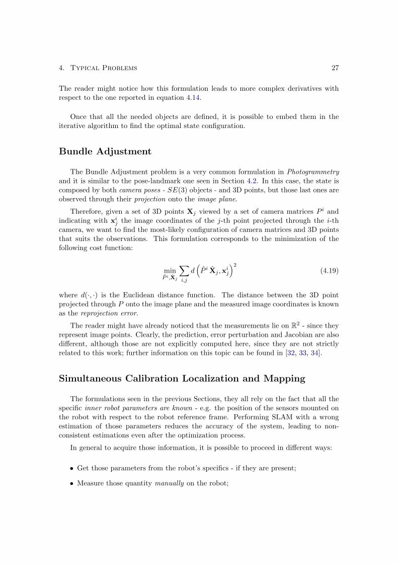
Bundle Adjustment
The Bundle Adjustment problem is a very common formulation in Photogrammetryand it is similar to the pose-landmark one seen in Section 4.2. In this case, the state iscomposed by both camera poses - SE(3) objects - and 3D points, but those last ones areobserved through their projection onto the image plane.
Therefore, given a set of 3D points Xj viewed by a set of camera matrices P i andindicating with xij the image coordinates of the j-th point projected through the i-thcamera, we want to find the most-likely configuration of camera matrices and 3D pointsthat suits the observations. This formulation corresponds to the minimization of thefollowing cost function:
minP i,Xj
∑i,j
d(P i Xj ,x
ij
)2(4.19)
where d(·, ·) is the Euclidean distance function. The distance between the 3D pointprojected through P onto the image plane and the measured image coordinates is knownas the reprojection error.
The reader might have already noticed that the measurements lie on R2 - since theyrepresent image points. Clearly, the prediction, error perturbation and Jacobian are alsodifferent, although those are not explicitly computed here, since they are not strictlyrelated to this work; further information on this topic can be found in [32, 33, 34].
Simultaneous Calibration Localization and Mapping
The formulations seen in the previous Sections, they all rely on the fact that all thespecific inner robot parameters are known - e.g. the position of the sensors mounted onthe robot with respect to the robot reference frame. Performing SLAM with a wrongestimation of those parameters reduces the accuracy of the system, leading to non-consistent estimations even after the optimization process.
In general to acquire those information, it is possible to proceed in different ways:
• Get those parameters from the robot’s specifics - if they are present;
• Measure those quantity manually on the robot;

4. Typical Problems 28
• Perform ad-hoc calibration before employing the robot in a mission.
All those procedures share the same drawbacks: they are not able to estimate non-stationary parameters and, if the robot is subject to hardware changes, the calibrationprocedure must be repeated.
A possible solution to this problem is to embed those parameters in the state and toestimate them together with the robot trajectory and the map. This solution has beenproposed by Kummerle et al. in their work [35] and it leads to several benefit to theoriginal SLAM problem. Therefore, in this Section it is proposed a brief overview of thisapproach.
Given a generic robot in a 2D environment, we have to introduce the following quan-tities:
• l = (lx ly θl) the pose of a generic sensor expressed with respect to the robot refer-ence frame;
• ui and Ωui that represent respectively the motion command and its relative infor-
mation matrix;
• k the parameters of the robot’s forward kinematic.
The forward kinematic function K(u,k) converts the wheels’ velocities deriving fromthe motion commands into the actual robot displacement from node i to i+1. For exam-ple, taking in consideration a differential drive kinematic scheme, the motion commandsmight be u = (vr vl)
T - respectively the left and right wheel velocity. Those lead to thefollowing relation to compute the relative motion obtained during a time step ∆t:
K(u,k) =
(R(∆t ω) 0
0 1
)(−ICC
0
)+
(ICC∆t ω
)(4.20)
where
ICC =
(0
b2rlvl+rrvrrlvl−rrvr
)ω =
rlvl − rrvrb
In this robot configuration rl and rr represent respectively the left and right wheel radii,while b is the distance between the two driving wheels. Those quantities represent theforward kinematic parameters k = (rr rk b)
T that we embed in the estimation process.
Given those objects, the optimization process has to retrieve the optimal configuration[x? l? k?] that minimizes the following negative log-likelihood function F (x, l,k):

4. Typical Problems 29
F (x, l,k) =∑i,j
elij(x)TΩlij elij(x) +
∑i
eui (x)T Ωli eui (x) (4.21)
where elij(x) describes how well the parameter blocks xi, xj and l satisfy the constraintzij , while eui (x) measures the likelihood of the parameter blocks xi, xj and k with respectto the constraint ui. The two error functions elij(x) and eui (x) are described analyticallyby the following relations:
elij(x) = ((xj l) (xi l)) zij
elij(x) = (xi+1 xi) K(ui,k)
where the operators and are the same of the ones described in the previous Sections.It is good to notice that, in order to obtain consistent results, the information matrix Ωu
i
must be projected through the forward kinematic function K(u,k), for example usingthe Unscented Transform [36].
Given the main notions about the most common formulations of the problem, inthe next Chapter it will be analyzed more in detail the solution for 3D factor graphs,explaining also the main contributions brought by this work.

Chapter 5
Solving Factor Graphs with SE3Variables
In this project it has been mainly addressed the optimization of 3D factor graphs.In particular it has been developed from scratch a back-end system to efficiently performpose and pose-landmark graph optimization.
The reader might feel already comfortable with the formulation of those problems,thus, in this Section will be shown more in detail the approaches used in order to achievereal-time performances and how SE(3) constraints have been manipulated in orderto reduce problem’s non-linearity.
Exploit Sparsity
As it as been already mentioned in Chapter 3, standard optimization algorithms likeGauss-Newton or Levenberg-Marquardt reduce the non-linear problem to the solution ofa linear system, namely:
H∆x = −b
Here, ∆x and b are dense vectors, while the Hessian’s approximation H is a sparsematrix. The literature proposes a lot of methods to solve efficiently sparse linear systems.Those can be categorized in two main groups:
1. Iterative methods [26] that compute a solution iteratively.
2. Direct methods [25] that solve the system in just one step.
The former ones like Conjugate Gradient or Generalized Minimal Residual Method -shortened as GMRES - exploit fast matrix-vector product to deliver good performanceseven if the solution is found iteratively. Those often use also preconditioning that consistin the application of a transformation - called the preconditioner - that turns the systeminto a form more suitable for numerical solving methods - e.g. Preconditioned ConjugateGradient (PCG). The latter group, instead, exploits matrix decompositions like Choleskyor the QR-decomposition to efficiently retrieve a solution in one step. Crucial for those
30

5. Solving Factor Graphs with SE3 Variables 31
kind of methods is the fill-in - i.e. the increase of non-zero elements in the decompositionwith respect to the source matrix.
Figure 5.1: Cholesky Fill-In. The figure highlights the fill-in due to the factorization of a(2000×2000) symmetric PSD matrix: non-zero blocks are depicted in white, while null-blocks inblack. The first row illustrates the patterns of matrices H and its decomposition L - respectivelyon the left and on the right. In the bottom row, the same matrices after the permutation ofH using the AMD ordering. It is clear the ordering contribution in reducing the fill-in of thefactorization, minimizing the memory required to store L and the number of block-matricesoperations.
As already mentioned in Section 3.3, variable reordering techniques, that consists inapplying a suitable permutation to the source matrix, are able to reduce dramatically

5. Solving Factor Graphs with SE3 Variables 32
the fill-in, allowing a faster decomposition. Several algorithm are proposed in literatureto compute the proper permutation - e.g. AMD, COLAMD. For the Cholesky LUdecomposition it is also possible to evaluate the pattern of the L matrix before computingthe actual decomposition, through the Symbolic Cholesky Decomposition. The readermight appreciate the variable reordering contribution in Figure 5.1.
In the remaining of the Section, it will be given a more detailed description on howto solve a sparse linear system using the Cholesky decomposition of the matrix H.
Storage Methods for Sparse Matrices
Another core aspect of sparse matrices is that there are several techniques to storethem more efficiently, reducing the amount of memory needed. The most general onesare Compressed Row Storage (CRS) or Compressed Column Storage (CCS), since they donot make any assumption on the structure of the matrix but the do not store unnecessaryelements - i.e. the zeros. Those method store the matrix using only 3 vectors: one vectorfor floating point numbers that represent the non-zero entries and two for the columnand row indexes respectively. As an example, given a matrix A
A =
10 0 0 0 −2 03 9 0 0 0 30 7 8 7 0 03 0 8 7 5 00 8 0 9 9 130 4 0 0 2 −1
in CRS format is represented by the following vectors - using zero-based indexing:
val =[10 −2 3 9 3 7 · · · 2 −1
]col =
[0 4 0 1 5 1 · · · 4 5
]row =
[0 2 5 8 12 16 19
]The vector row contains the indexes of the elements that correspond to the first non-zeroentry of each row in the sparse matrix A.
List of Lists (LIL) represents another effective and easy-to-implement storage method.In this case, each row-vector is represented as a list of pairs that denotes the columnindex and the element’s value.
Recalling equation 3.24, since in this problem it has been considered only binaryconstraints, the linearization of each edge generates 4 block-contributions to the Hessian,namely:

5. Solving Factor Graphs with SE3 Variables 33
Hii = JTi Ωk Ji Hjj = JTj Ωk Jj
Hij = JTi Ωk Jj Hji = JTj Ωk Ji
Therefore, the Hessian can be intended to be a sparse block-matrix where each entryis a matrix itself of a given size. In our work, it has been chosen to employ the LILstorage method with block-entries, in order to speed-up the numerical computations -better explained in the next Chapter.
Cholesky Decomposition
In linear algebra, the Cholesky decomposition (or factorization) is the decompositionof a Hermitian, positive semi-definite (PSD) matrix into the product of a lower triangularmatrix and its conjugate transpose, namely:
A = L L? (5.1)
In this particular problem formulation, the matrices involved are composed by real num-bers, therefore the conjugate transpose of L becomes its transposed LT = U. In thissense, it represents the square-root operator for symmetric PSD matrices.
A more stable variant of the classical Cholesky decomposition is the LDL decompo-sition. In this case, the original matrix is decomposed into the following product:
A = LDL? (5.2)
where L is a lower unit triangular matrix - i.e. all the entries on the main diagonal are1 - and D a diagonal matrix. This variant requires the same space and computationaleffort with respect to the original one but avoids the square-roots extraction. In thisway, even matrices that do not have a Cholesky decomposition can be factorized withthe LDL one. However, in this work, since the matrices take into account are symmetricand PSD by construction, it has been chosen the original Cholesky decomposition.
In general the computational complexity for the factorization of a (n× n) matrix isO(n3), requiring about n3/3 FLOPs. There are several algorithm available to compute thefactorization, however, one of the most common is the Cholesky-Banachiewicz. In thisalgorithm the computation starts from the top-left corner of the matrix L and proceedsthe computation row-by-row as follows:
A = LLT =
L00 0 0L10 L11 0L20 L12 L22
L00 L10 L20
0 L11 L21
0 0 L22
where

5. Solving Factor Graphs with SE3 Variables 34
Ljj =√Ajj −
∑j−1k=1 L
2jk
Lij = 1Ljj
[Aij −
∑j−1k=1 Lik Ljk
]for i > j
(5.3)
The Cholesky-Crout ’s algorithm, instead, is a column-wise version of the previousone. It is good to notice that both algorithms allow to perform the computation alsoin-place. Moreover, both algorithms can be employed in sparse block-matrices, leadingto a block-Cholesky factorization. The blocks are also computed as in Equation 5.3 but,in the block case, the square root operator is applied to the matrix-block and it consistsin the Cholesky decomposition of the block itself.
As it has been already mentioned, the main use of the Cholesky decomposition is inthe solution of linear systems. Given a symmetric PSD real matrix A, the solution ofthe linear system A x = b is computed through the following steps:
1. Cholesky factorization of the source matrix A = LLT
2. Forward substitution to solve the linear system L y = b
3. Backward substitution to solve the linear system LT x = y
Clearly, since in the problem in analysis H and its factorization L are sparse block-matrices, also b and y are dense block-vector - with the number of blocks N equal to thenumber of vertexes in the graph.
Manifold Representation
As it has been already stated at the begin of the Chapter, this work focuses on3D formulations of pose and pose-landmark graphs. In this Section it will be betteranalyzed the representation of all the objects required for the LS estimation in both theformulations.
3D Pose-Graph
Pose-graph optimization in 3D represents the backbone of SLAM, allowing to estimatethe robot trajectory in space through MAP estimation. In this formulation, the statex includes the 3D orientation of the nodes which represent the main reason why pose-SLAM is a complex problem. Rotations in space can be over-parametrized through a 3Drotation matrix R ∈ SO(3). Therefore, the over-parametrized state can be representedby a 3D isometry X = WTR ∈ SE(3) which represents the robot pose in the worldreference frame - i.e. a (4× 4) homogeneous transformation matrix.
A possible minimal representation of the state can be a 6 vector x = (tx ty tz αβ γ)T ,where the triplet r = (αβ γ)T represents the Euler Angles that compose the rotational
5. Solving Factor Graphs with SE3 Variables 35
part of the isometry, while t = (tx ty tz)T is the translational one. Summarizing, in
formulæ:
X =
(R t0T 1
)x =
[tx ty tz α β γ
]Twhere
R = Rx(α) Ry(β) Rz(γ) (5.4)
The measurements are also of type pose, thus, it is possible to use the same notationthat describes the state. Therefore Zij represents the over-parametrized measurement ofnode j with respect to node i - i.e. a 3D isometry iTj .
The next required step concerns the definitions of suitable operators box-plus andbox-minus. We introduce again the operators v2t and t2v that allow to map the over-parametrized representation into the minimal one and vice versa. Those two operatorsallow to define the following relations:
X ∆x = v2t(∆x) X (5.5)
Xa Xb = t2v(X−1b Xa
)(5.6)
For SE(3) object, the v2t function computes the rotational part of X through Equation5.4 and then composes the isometry adding the translational part t = (tx ty tz)
T . InEquation 5.4 the factors Rx, Ry and Rz represent the 3D rotation respectively aroundthe x, y and z axis; they are defined as follows:
Rx(α) =
1 0 00 cosα − sinα0 sinα cosα
(5.7)
Ry(β) =
cosβ 0 sinβ0 1 0
− sinβ 0 cosβ
(5.8)
Rz(γ) =
cos γ − sin γ 0sin γ cos γ 0
0 0 1
(5.9)
Instead, to retrieve the Euler given the rotation matrix R - that is done in the t2voperator - it is necessary to equate each element in R with its corresponding element inthe matrix product Rx(α) Ry(β) Rz(γ), in formulæ:

5. Solving Factor Graphs with SE3 Variables 36
R =
R00 R01 R02
R10 R11 R12
R20 R21 R22
= Rx(α) Ry(β) Rz(γ) = (5.10)
=
cosβ cos γ − cosβ sin γ sinβcosα sin γ + sinα cos γ sinβ cosα cos γ − sinα sinβ sin γ − cosβ sinαsinα sin γ − cosα cos γ sinβ sinα cos γ + cosα sinβ sin γ cosβ cosα
The reader might notice the non-linearities introduced by the functions t2v and v2t.
Those imply the computation of complex non-linear derivatives to retrieve the Jacobianin the linearization phase. However, this problem - and the solution proposed in thiswork - will be better analyzed in the next Section.
3D Pose-Landmark
In this formulation, as already explained in Section 4.3, the system has to estimateboth the robot trajectory and the position of salient world points - i.e. the 3D landmarks.Therefore, the system’s state and increment are described as follows:
X =
Nposes
XR1 , ...,X
RN |
Mlandmarks
xLN+1, ...,xLN+M
∆x =
Nposes
∆xR1 , ...,∆xRN |Mlandmarks
∆xLN+1, ...,∆xLN+M
The formalization for SE(3) nodes remains unchanged from the previous Subsection,
therefore, it is necessary to characterize only the nodes that describe the landmarks.
Landmarks’ nodes lie on R3, so it is not necessary to define anything else - i.e. nobox-plus/box-minus operator needed. As a consequence of this, a measurement zij ∈ R3
is a simple 3 vector that describes the position of point j in the i-th pose reference frame.
However, it is necessary to consider also the fact that the sensor’s reference frameand the robot’s one might not coincide, but they are related through the transformationS = RTS ∈ SE(3). Thus, given the state, the predicted measurement is:
zij = hij(X) = S−1 X−1i
K
pj = RKpj + tK (5.11)
In light of this, without loss of generality, the error between the predicted and the actualmeasurement is computed as follows:

5. Solving Factor Graphs with SE3 Variables 37
eij = zij − zij = S−1X−1i pj − zij (5.12)
Given Equation 5.12, the perturbed error will be:
eij(Xi ∆xRi ,xj + ∆xLj ) = S−1[(
v2t(∆xRi )Xi
)−1 (pj + ∆xLj
)]− zij (5.13)
Finally, it is necessary to compute the Jacobian J deriving from the constraint zij ,that is structured as follows:
J = [0 · · · 0 JR 0 · · · 0 JL 0 · · · 0]
where
JR =∂ S−1
[(v2t(∆xRi )Xi
)−1(pj + ∆xLj
)− zj
]∂∆xRi
∣∣∣∣∣∆xRi = 0
∆xLj = 0
=
=∂[RTS
[v2t(∆xRi )Xi
]−1pj −RT
StS
]∂∆xRi
∣∣∣∣∣∆xRi = 0
∆xLj = 0
=
=∂RT
SX−1i
[v2t(∆xRi )
]−1pj
∂∆xRi
∣∣∣∣∣∆xRi = 0
∆xLj = 0
=
=∂[RTS RT
R
[v2t(∆xRi )
]−1pj −RT
R tR
]∂∆xRi
∣∣∣∣∣∆xRi = 0
∆xLj = 0
=
=∂RT
S RTR
([v2t(∆xRi )
]−1pj
)∂∆xRi
∣∣∣∣∣∆xRi = 0
∆xLj = 0
= RTS RT
R
∂[R∆xR
ipj −R∆xR
it∆xR
i
]∂∆xRi
∣∣∣∣∣∆xRi = 0
∆xLj = 0
Exploiting the fact that the derivative expressed in the previous equation is evaluated in∆xRi = 0, it leads to the following relation:
JR = RTS RT
R
[−I3×3 | −bpjc×
](5.14)
The other component of J - namely JL - instead can be computed as follows:

5. Solving Factor Graphs with SE3 Variables 38
JL =∂ S−1
[(v2t(∆xRi )Xi
)−1(pj + ∆xLj
)− zj
]∂∆xLj
∣∣∣∣∣∆xRi = 0
∆xLj = 0
=
=∂[RTS X−1
i
(pj + ∆xLj
)−RT
S tS
]∂∆xLj
∣∣∣∣∣∆xRi = 0
∆xLj = 0
=
=∂[(
RTS X−1
i pj)
+(RTS X−1
i ∆xLj
)]∂∆xLj
∣∣∣∣∣∆xRi = 0
∆xLj = 0
= RTS
∂[RTR ∆xLj −RT
RtR
]∂∆xLj
∣∣∣∣∣∆xRi = 0
∆xLj = 0
This result - expanding the derivatives and exploiting that the linearization point is∆xLj = 0 - leads to the following relation:
JL = RTS RT
R (5.15)
The reader might notice that JR is a (3 × 6) matrix - since the minimal representationof SE(3) states has 6 components - while JL is a (3× 3) matrix - because R3 states arevectors with only 3 components.
In the next Section it is proposed a deeper analysis on the error representation andthe linearization of 3D pose constraints, highlighting the non-linearity of the computationand the proposed approach to overcome this issue.
Dealing with SE3 Objects
3D poses are complex objects to manage, due to their rotational part that introducesmany an highly non-linear contribution in the linearization process. In this sectionit is proposed an approach that aims to reduce those non-linearities while deliveringperformances comparable to other state-of-the-art systems.
Chordal Distance Based Error Function
Recalling 5.2.1, we have defined the functions v2t and t2v that allow to map the min-imal representation of the state into the redundant one and vice-versa. Through them,we defined the operators box-plus and box-minus, described respectively in Equations 5.5and 5.6. Sticking to this notion, the predicted measurement Zij of pose j from pose i iscomputed as
Zij = hij(X) = X−1i Xj (5.16)

5. Solving Factor Graphs with SE3 Variables 39
that leads to the following error function:
eij(X) = Zij Zij = t2v(Z−1ij X−1
i Xj
)(5.17)
The error eij is a 6 vector that expresses the mismatch of each component of state’sminimal representation. Proceeding with the error perturbation, the result will be:
eij(Xi ∆xi,Xj ∆xj) = t2v(Z−1ij (v2t(∆xi) Xi)
−1 (v2t(∆xj) Xj))
(5.18)
The full Jacobian J = [0 · · · 0 Ji 0 · · · 0 Jj 0 · · · 0] will be quite complex to com-pute due to the derivative of the t2v and v2t functions, requiring also many FLOPs and,thus, slowing the optimization process. In this formulation Ji and Jj are (6×6) matrices.
It is possible to approach this problem using a different error formulation that leadsto easy-to-compute derivatives. In order to do so, we define the Lp,q norm of a (m× n)matrix A as follows:
‖A‖p,q =
n∑j=1
(m∑i=1
|aij |p)q/p
1/q
For p = q = 2 the becomes
‖A‖F =
n∑j=1
(m∑i=1
|aij |2)2/2
1/2
=
√√√√ m∑i=1
n∑j=1
|aij |2 (5.19)
that represents the Frobenius norm of a matrix, an entrywise norm, which is also invari-ant under rotation constraint. Based on this concept, it is possible to define the chordaldistance between two rotation matrix RA and RB as follows:
dchord(RA,RB) = ‖RA −RB‖F (5.20)
It is good to notice that the difference operator employed in Equation 5.20 is the standardEuclidean minus, executed element-wise.
We define also a new function, that given a 3D isometry returns a 12 vector madewith its components, namely:

5. Solving Factor Graphs with SE3 Variables 40
Manifold curvature
ApproximatedLine Segment
p1
p2
p1
p2
Figure 5.2: Chordal Distance. This figure shows the underlying concept of the new errorfunction: the distance between p1 and p2 can be approximated with the Euclidean distancecomputed between the projection of those points onto the relative chord - namely between p1
and p2.
X =
[R t0 1
]R =
(r1|r2|r3
)flatten(X) =
r1
r2
r3
t
(5.21)
where rk represents the k-th column of R.
Finally, we introduce the following relations to express operators box-plus and box-minus:
X ∆x = v2t(∆x) X (5.22)
Xa Xb = flatten (Xa)− flatten (Xb) (5.23)
5. Solving Factor Graphs with SE3 Variables 41
Given those mathematical concepts, it is possible to define the error between twoSE(3) objects through a relaxed version of the chordal distance, that leads to the fol-lowing relations:
Zij = hij(X) = flatten(X−1i Xj
)(5.24)
eij(X) = Zij − Zij = flatten(X−1i Xj
)− flatten (Zij) (5.25)
It is good to notice that eij now is a 12 vector, therefore, the Jacobian’s components Jiand Jj will be (12 × 6) matrices. Speaking about this, applying the state perturbationto the error will lead to the following relation:
eij(Xi ∆xi,Xj ∆xj) = flatten(
(v2t(∆xi)Xi)−1 (v2t(∆xj)Xj)
)− flatten (Zij)
(5.26)
It is already possible to notice the reduced complexity of the derivatives required tolinearize the constraint. In fact, from Equation 5.26 it is possible to retrieve the followingrelations - stating that R∆xi = Rx
∆xiRy
∆xiRz
∆xi:
Jj =∂ eij(Xi ∆xi,Xj ∆xj)
∂∆xj
∣∣∣∣∣∆xi = 0∆xj = 0
=
=
∂
flatten
G[
RTi −RT
i ti0 1
][(Rx
∆xiRy
∆xiRz
∆xi
)T−RT
∆xiti
0 1
] [Rj tj0 1
]
∂∆xj
∣∣∣∣∣∆xi = 0∆xj = 0
Expanding the derivatives, it is possible to define the following - intuitively retrieved -objects:
• R′x0, R′y0 and R′z0 that represent derivatives with respect to ∆α, ∆β and ∆γ ofthe base rotation Rk(·), evaluated in 0 and with k = x, y, z;
• R′x0, R′y0, and R′z0 that are the derivatives with respect to ∆α, ∆β and ∆γ of the
rotational part of matrix G, computed as R′k0 = RTi R′k0 Rj with k = x, y, z;
• r′k0 which describes the 9 vector obtained stacking the columns of R′k0 - withk = x, y, z.
In the light of what we just stated, it is possible to retrieve this final formulation of Jj :

5. Solving Factor Graphs with SE3 Variables 42
Jj =
(0(9×3)
[r′x0 | r′y0 | r′z0
](9×3)
RTi −RT
i btjc×
)(5.27)
Intuitively, the other component of the Jacobian will be simply
Ji = −Jj (5.28)
The reader might noticed how the new error function reduced the computational costof the derivatives, due to the elimination of the highly non-linear function t2v. Moreover,the use of standard Euclidean minus operator to express differences between transforms,leads to a better approximation by the first-order Taylor expansion of the perturbederror. This better approximation enlarges the converge basin of the optimization processand it improves the avoidance of local minima.
Benefits in the Re-linearization
The reader might remember that, since also the measurements live on a non-Euclideanspace, it is necessary to project the measurement information matrices through the box-minus operator. Therefore, using the standard box-minus described in Equation 5.6 andgiven Zij associated to Zij = Zk, it is required to compute the following objects at eachiteration of the LS optimization:
JZk=∂(Zij Z
)∂Z
∣∣∣∣Z=Zk
(5.29)
Ωk =(JZk
Ωk JTZk
)−1(5.30)
The error function based on the chordal distance that has been proposed in the pre-vious Sub-section, brings benefits also in this sense. In fact, since the operator employedto compute the error is the standard Euclidean minus, it is not required to recomputethe information matrix Ωk at each iteration.
It is good to notice that the information matrix associated with the measurement Zkis a (6× 6) matrix Ωk , since the state’s minimal representation has dimension 6 in thisformalization. However, it is necessary to consider the contribute of function flatten (·)in this process: the new error space has dimension 12, thus it is necessary to projectthe information matrix into the new higher dimensional space. To this end, it will beproposed now some new mathematical concepts useful in order to estimate the result ofapplying a non-linear transformation to a probability distribution function.
Given a Gaussian distribution p(x) = N (x;µ,Σ) with mean µ and covariance Σ, itis possible to represent it through a set of weighted points called Sigma Points. EachSigma Point χi is described by a set of parameters:

5. Solving Factor Graphs with SE3 Variables 43
• a position xi
• a weight for the mean wim ∈ R+
• a weight for the covariance wic ∈ R+
Clearly, the conversion from the original parameters (µ,Σ) to the Sigma Points χi =(xi, wim, w
ic) must be invertible. In fact, it is possible to reconstruct the Gaussian param-
eters from the Sigma Points as follows:
µ =∑i
wim xi (5.31)
Σ =∑i
wic (xi − µ)(xi − µ)T (5.32)
It is good to notice that, if the original Gaussian distribution has dimension n, asuitable number of Sigma Point required to approximate it without loosing informationwill be N = 2n + 1. In order to control how far the Sigma Points are sampled fromthe mean µ though, it is possible to tune the scalar parameters κ ∈ R+ and α ∈ (0, 1].Therefore, the position of each Sigma Point is computed as follows:
x(0) = µ (5.33)
x(i) =
µ+ [L]i for i ∈ [1 . . . n]
µ− [L]n−i for i ∈ [n+ 1 . . . 2n](5.34)
where L =√
(n+ λ)Σ and λ = α2(n+κ)−n. Given the scalar parameter β = 2 - tunedfor Gaussian PDFs - the weights are retrieved as follows:
w(0)m =
λ
λ+ n(5.35)
w(0)c = w(0)
m + (1− α2 + β) (5.36)
w(i)c = w(i)
m =1
2(n+ λ)(5.37)
This transformation between actual Gaussian parameters and the Sigma Points iscalled Unscented Transform [36]. The core feature of this mathematical functionis that it can be used to apply a transformation to a PDF in a straightforward way.Sticking to Gaussian PDFs, given Xa ∼ N (xa;µa,Σa) and its Unscented Transform
xa ∼ UT (xa;x(i)a , w
(i)m , w
(i)c ), computing the Gaussian Xb = g(Xa) can require a lot of
effort. However, a good approximation of Xb can be computed applying the functiong(·) to the Unscented Transformation of Xa. This translates in the application of theg(·) function to each Sigma Point of xa, namely
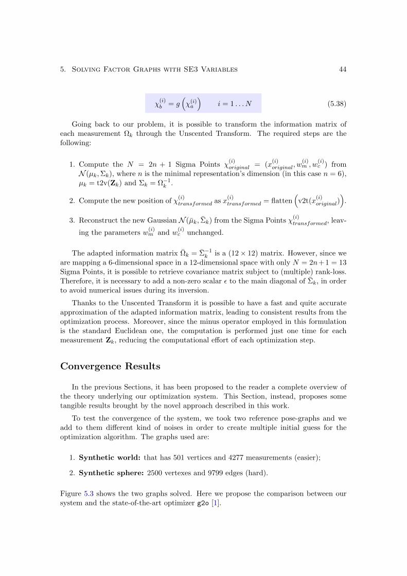
5. Solving Factor Graphs with SE3 Variables 44
χ(i)b = g
(χ(i)a
)i = 1 . . . N (5.38)
Going back to our problem, it is possible to transform the information matrix ofeach measurement Ωk through the Unscented Transform. The required steps are thefollowing:
1. Compute the N = 2n + 1 Sigma Points χ(i)original = (x
(i)original, w
(i)m , w
(i)c ) from
N (µk,Σk), where n is the minimal representation’s dimension (in this case n = 6),µk = t2v(Zk) and Σk = Ω−1
k .
2. Compute the new position of χ(i)transformed as x
(i)transformed = flatten
(v2t(x
(i)original)
).
3. Reconstruct the new Gaussian N (µk, Σk) from the Sigma Points χ(i)transformed, leav-
ing the parameters w(i)m and w
(i)c unchanged.
The adapted information matrix Ωk = Σ−1k is a (12× 12) matrix. However, since we
are mapping a 6-dimensional space in a 12-dimensional space with only N = 2n+1 = 13Sigma Points, it is possible to retrieve covariance matrix subject to (multiple) rank-loss.Therefore, it is necessary to add a non-zero scalar ε to the main diagonal of Σk, in orderto avoid numerical issues during its inversion.
Thanks to the Unscented Transform it is possible to have a fast and quite accurateapproximation of the adapted information matrix, leading to consistent results from theoptimization process. Moreover, since the minus operator employed in this formulationis the standard Euclidean one, the computation is performed just one time for eachmeasurement Zk, reducing the computational effort of each optimization step.
Convergence Results
In the previous Sections, it has been proposed to the reader a complete overview ofthe theory underlying our optimization system. This Section, instead, proposes sometangible results brought by the novel approach described in this work.
To test the convergence of the system, we took two reference pose-graphs and weadd to them different kind of noises in order to create multiple initial guess for theoptimization algorithm. The graphs used are:
1. Synthetic world: that has 501 vertices and 4277 measurements (easier);
2. Synthetic sphere: 2500 vertexes and 9799 edges (hard).
Figure 5.3 shows the two graphs solved. Here we propose the comparison between oursystem and the state-of-the-art optimizer g2o [1].

5. Solving Factor Graphs with SE3 Variables 45
(A)
(B)
Figure 5.3: Solved Graphs Top image: the synthetic world graph solved. Bottom: syntheticsphere solved.
The first test done consisted in applying the noise only on the translational part ofthe nodes; the employed graph is the synthetic world - Figure 5.3A. Obviously, both thesystem preformed well recreating the original graph, as shown in Figure 5.4.
However, our system claims to be more effective to manipulate rotations. Conse-quently, the second test focused on this: the initial guess, in fact, was created fromthe synthetic world graph adding white noise - i.e. sampled from N (0, 1) - only to therotation R of each node.
With this initial guess, g2o suffers from the non-linearities introduced by the v2t andt2v functions as the reader might notice in Figure 5.5A. To confirm the qualitative resultobtained, we decided to compare g2o’s chi2 with the one obtained with our approach,

5. Solving Factor Graphs with SE3 Variables 46
Figure 5.4: Translational Noise. From left to right: initial guess, g2o solution, our solution.Both the approaches generate consistent results.
(A)
1 2 3 4 5 6 7 8 9 10 11iteration
105
106
107
108
chi2
g2oour
(B)
Figure 5.5: Rotational Noise. Figure (A) from left to right: initial guess, g2o solution, oursolution. Figure (B) shows the chi2 of both approaches at each iteration: it is clear the conver-gence gap between g2o - in blue - and our approach - in orange. The y axis’ scale is logarithmic.The iterations performed are 10, therefore, the point x = 1 indicates the chi2 of the initial guess.
iteration by iteration. In order to obtain comparable objects - and to not bias thecomparison - it has been saved the graph obtained with our system at each iteration and

5. Solving Factor Graphs with SE3 Variables 47
evaluated its initial chi2 in g2o. The result of this comparison is shown in figure 5.5B.
In order to further confirm the quality of the chosen approach, is has been gen-erated another initial guess for the same graph, but the noise figure was sampled fromN (0, 1000). In this case both the systems struggle to find a solution in only 10 iterations,but the trend is better with our error function - see Figure 5.6.
(A)1 2 3 4 5 6 7 8 9 10 11
iteration
107
108
chi2
g2oour
(B)
Figure 5.6: Advanced Rotational Noise. Figure (A) from left to right: initial guess, g2o
solution, our solution. Figure (B) shows the chi2 of both approaches at each iteration. g2o’strend might indicate that the system got stuck in a local minimum.
The next step consists in applying both noise figures to the sphere graph, togetherwith a translational perturbation (therefore a 6 DoF noise vector), generating a veryharsh initial guess.
Given the complexity of the initial guess, we decided to perform more iterations withrespect the previous graph - i.e. 100. Figure 5.7 shows the qualitative and quantitativeresults of both g2o and our approach, after applying 6 DoF Gaussian noise - sampled fromN (0, 1). The reader might appreciate the fact that g2o converges to a local minimumfar from the optimum, instead, our approach is able to reach the optimum in lessthan 40 iterations.
Finally, in the last test it has been increased the rotational component of the noise,which, in this extreme case, is sampled from N (0, 1). Here, without a kernel both thesystems struggles to optimize the graph.
Figure 5.8 shows the outcomes of both the systems: clearly neither g2o nor oursystem reached the optimum, however the solution retrieved with the proposed methodis evidently more consistent.
In Subsection 5.3.2, it has been highlighted that converting the information matri-ces from a 6-dimensional space to a 12-dimensional one through the Unscented Trans-form may generate multiple rank loss, thus, the matrix Σk = Ω−1
k must be conditionedsomehow to avoid singularities. Given this, it has been tested the effects of differentconditioning methods, however the most promising ones where basically 3:
1. Soft Conditioning. It is computed the Singular Value Decomposition of matrixΣk = UDV ?, then it is added a non-zero value ε only to the degenerated eigenvaluesand finally it is computed the matrix Σconditioned
k = UDV ?.
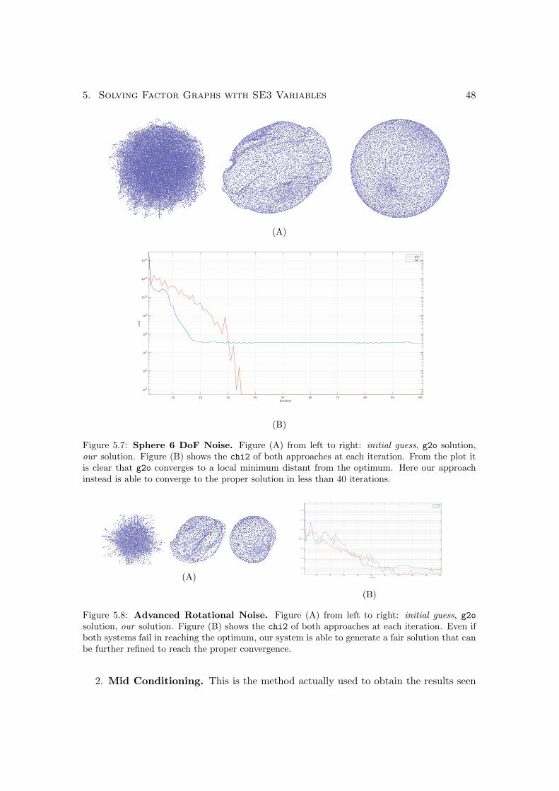
5. Solving Factor Graphs with SE3 Variables 48
(A)
10 20 30 40 50 60 70 80 90 100iteration
105
106
107
108
109
1010
1011
1012
chi2
g2oour
(B)
Figure 5.7: Sphere 6 DoF Noise. Figure (A) from left to right: initial guess, g2o solution,our solution. Figure (B) shows the chi2 of both approaches at each iteration. From the plot itis clear that g2o converges to a local minimum distant from the optimum. Here our approachinstead is able to converge to the proper solution in less than 40 iterations.
(A) 10 20 30 40 50 60 70 80 90 100iteration
108
109
1010
1011
1012
1013
1014
chi2
g2oour
(B)
Figure 5.8: Advanced Rotational Noise. Figure (A) from left to right: initial guess, g2o
solution, our solution. Figure (B) shows the chi2 of both approaches at each iteration. Even ifboth systems fail in reaching the optimum, our system is able to generate a fair solution that canbe further refined to reach the proper convergence.
2. Mid Conditioning. This is the method actually used to obtain the results seen

5. Solving Factor Graphs with SE3 Variables 49
until now, and consists in applying a non-zero value ε to all the elements on thediagonal of Σk. Reasonable values are ε ∈ [10−2, 10−4].
3. Hard Conditioning. In this case, all the values outside the main diagonal aresimply ignored - i.e. set to zero.
Figure 5.9: Conditioning Methods. The outcomes of the three conditioning methods used tocompute the measurements’ information matrix. Given the initial guess relative to Figure 5.7A,from left to right are illustrated: soft, mid and hard conditioning.
This comparison opens a new path for further investigations, in order to retrieve thebest conditioning method to compute the measurements’ information matrices.
As this Section showed, the novel features introduced so far lead to an accurate andmore robust optimizer, that delivers results comparable or better to other state-of-the-art systems. In the next Chapter, the reader will have an insight on the actualimplementation of the system, in order to better understand how all those mathematicalconcepts have been applied in practice and to show the speed performances reached byour system.

Chapter 6
Software Implementation of theOptimizer
This Chapter will better analyze the actual implementation of a 3D Optimizer. Inparticular, it has been developed a self-consistent C++ library that provides all the toolsneeded to create and optimize 3D graphs that contain pose or point objects. The maincomponents of the system are basically two:
1. The Optimizer itself that runs the Gauss-Newton algorithm to retrieve the beststate configuration given the constraints.
2. The Graph, that contains the actual nodes and edges generated by a suitable front-end or read from file.
While the Graph is just a container for nodes and edges, the optimizer has to performseveral computations in order to retrieve the linear system H∆x = −b and then solveit. Therefore, underlying the optimizer a linear solver is required to efficiently solve theaforementioned system.
Once that the front-end populates the graph (or it is loaded from a file), it is fed asinput of the optimizer; the general work-flow of a graph optimizer is the following:
1. Linearization: for each edge it is computed the error with respect to the currentsystem state and then the relative Jacobian. The output of this phase is thecontribution of the edge to the Hessian matrix and the right-hand-side vector.
2. Permutation: once that the Hessian H is built, it is necessary to compute a properpermutation to reduce Cholesky factorization’s fill-in and apply it to Hessian andthe right-hand-side vector.
3. Linear Solver: now it is possible to compute the actual Cholesky factorization Land retrieve ∆x via Forward/Backward Substitution.
4. Update: finally, once that ∆x is computed, it is possible to apply it to the currentsystem state - i.e. to all the graph’s Vertex.
50

6. Software Implementation of the Optimizer 51
It is good to notice that our system is almost completely self-contained: the onlyexternal libraries employed are Eigen [37] - to efficiently manage small matrices - andSuiteSparse [38] - in order to compute the right permutation of the Hessian. Furthermore,the library has been developed with simplicity and keeping a minimalistic approach, inorder to be comprehensible also by researchers that are not expert in this field. Just forcomparison, the entire library has less than 6 thousand lines of code; other state-of-the-art systems are deployed in huge libraries with thousands of lines of code - e.g. g2o [1] isover 40 thousands lines of code, Ceres [39] is over 90 thousands lines of code and gtsam
[19] over 300 thousands lines of code.
Graph
The Graph is basically constituted by a collection of edges and nodes. The nodes canbe either of type pose or point - represented respectively by the objects VertexSE3 andVertexR3. Each vertex is represented by
• Its estimate, which can be a 3D isometry or a 3D position - namely a Pose3D ora Point3D;
• A unique index that is used to recognize the vertex;
• A boolean variable that indicates whether the node is fixed or not. A fixed Vertexmust not be involved in the optimization process. It is good to notice that at leastone fixed vertex must exists in the graph, otherwise the optimization problem isundefined.
Analogously, the edge are of type pose-pose or pose-point - represented respectivelyby the objects EdgeSE3 and EdgeSE3 R3. The edge have several fields, namely:
• The actual measurement that can be either a Pose3D or a Point3D;
• The data association that consists in a pair of Vertex which represents the nodesinvolved in the edge;
• The information matrix related to the measurement - namely a Matrix6 or aMatrix3.
Once that the front-end populates the graph, it is fed into the Optimizer to performMAP estimation of the best state configuration given the constraints.
The Optimizer
The Optimizer represents systems’ heart: it takes as input the graph, retrieves thelinear system H∆x = −b, solves for ∆x and finally updates the graph. In the followingSubsections the core elements of the Optimizer will be better investigated.

6. Software Implementation of the Optimizer 52
Linearization and Hessian Composition
One of Optimizer’s tasks is to compute the contribution that each edge brings toboth the Hessian matrix H and the right-hand-side vector b. Those contribution areretrieved during the linearization of the graph.
Each edge of the graph is analyzed, whether it is a EdgeSE3 or a EdgeSE3 R3. Foreach measurement the block matrices Hii, Hij , Hji and Hjj are computed as
Hii = JTi ΩkJi Hjj = JTj ΩkJjHij = JTi ΩkJj Hji = JTj ΩkJi
(6.1)
while the right-hand-side contributions are computed as
bi = JTi Ωkek bj = JTj Ωkek (6.2)
The subscript indexes 〈i, j〉 are the node unique indexes in the current edge’s data-association. The tuple 〈i, j〉 indicates the position of each block in the full Hessian H(and in the full right-hand-side vector b).
The Jacobians Ji and Jj are using Equations 5.28 and 5.27 for pose constraints,while for point ones Equations 5.14 and 5.15. Clearly, as reported in Section 5.3, theinformation matrix of each EdgeSE3 is adapted through the Unscented Transform beforestarting the optimization process - and not at each iteration.
Sparse Linear Solver
The linear solver employed is based on Cholesky decomposition of the Hessian - i.e.Subsection 5.1.2. Clearly, the first thing needed in order to efficiently solve a sparselinear system is a proper matrix data-structure.
In this work, sparse matrices are represented through the SparseBlockMatrix ob-ject, which uses as storage method the List of Lists (LIL) approach. It is possible toselect between fixed-size blocks - i.e. in pose graph optimization - and dynamic blocks -i.e. in pose-landmark graph optimization. In the former case it is possible to take advan-tage of CPU cache while doing matrix operations and, thus, boosting the computation;using dynamic blocks matrix operations are slower but it adds flexibility to the system.SparseBlockMatrix main feature is the fact that object’s memory - used to actuallystore the blocks - can be isolated from the objects itself. Therefore, the actual matrixis just a view of those blocks, intended as a LIL of pointers to those memory blocks.This formulation allows to manipulate the SparseBlockMatrix without touching thememory, just rearranging matrix’s view. The object DenseBlockVector is designed onthe basis of this and it used to store dense vectors like the right-hand-side vector b andthe update vector ∆x.
Before computing the Cholesky factorization, Hessian’s non-zero pattern is analyzedthrough the SuiteSparse library in order to retrieve a suitable ordering that reduces

6. Software Implementation of the Optimizer 53
Cholesky’s fill-in. The user can choose between different algorithms - i.e. AMD, CO-LAMD, CHOLMOD - or let the system retrieve the best one.
Once the permutation is found, SparseBlockMatrix’s view of matrix H is rearrangedbased on the permutation, together with the DenseBlockVector b. Now it is possible tocompute the Cholesky factorization and retrieve the matrices L and LT . Finally, throughForward-Backward Substitution, the update vector ∆x is found.
It is good to notice that before solving the linear system, it is necessary to removefixed vertexes’ contribution from the system. Supposing that node f is fixed, then it isnecessary to remove the f -th row and column from the Hessian, together with the f -thblock of the b. Therefore the system we solve has dimension n− F , where F representsthe number of fixed vertexes.
Graph Update
Once that the DenseBlockVector ∆x is computed, it is necessary to apply to eachnode k the relative block ∆xk of the update vector.
The update is applied node by node through the box-plus operator described inEquations 5.22 for SE(3) nodes and the Euclidean minus for R3 ones. Clearly, fixednodes will remain unchanged.
Bottlenecks
The system has been designed to deliver real-time performances, therefore, an ad-hocimplementation is required to achieve such result. The system described in the previousSection has two main time-consuming operations, both performed at each iteration:
1. Allocation and management of the memory for the Hessian’s blocks;
2. The actual computation of the Hessian’s blocks described in Equation 6.1.
However, the proposed system tackles both the issue, reducing the time required foreach iteration to values comparable to state-of-the-art systems.
Memory management
Allocate the memory blocks for the Hessian H is a time-expensive operation. Fur-thermore, it is required to allocate memory also for its decomposition L and LT and forthe dense vector b, ∆x and y. Moreover, copying memory - for example to create apermutation of a matrix - is another time and resource consuming operation.
The memory copy has been addressed through the separation of matrix view andmemory in the SparseBlockMatrix object, as mentioned before. In this way it is possibleto create multiple views of a matrix that share the same physical memory, avoiding

6. Software Implementation of the Optimizer 54
memory copy and, thus, reducing the memory consumption of the system. The samefeature is found in the DenseBlockVector object. The physical memory is managed bya separated object called MemoryManager. It is in charge of allocating, delete and copymemory for matrix and vectors.
However, even if we are able to avoid memory copy, it is necessary to allocate thematrices and vectors at each iteration. Once again, this process is avoided through aclever solution: once the graph is built, it is possible to exploit its structure to evaluatethe non-zero pattern of the Hessian H. The reader might notice that the non-zero patternwill remain unchanged for the entire optimization process, while the numeric values ofthe block will change at each iteration. Moreover, all the DenseBlockVectors will have afixed dimension equal to the number of active vertexes n−F . Therefore, it is possible toallocate all the memory required to store Hessian’s and vectors’ block only once beforestarting the optimization process.
Once that we have the Hessian’s non-zero pattern, it is possible to compute boththe permutation and the Cholesky symbolic decomposition, that retrieves the non-zeropattern of matrix L (and thus also LT ). In this way, during the optimization steps thereis no memory allocation or copy, speeding up the entire system.
Hessian blocks computation
Using the Eigen library to perform matrix operations, it is possible to appreciate abottleneck in the computation of the product Hij = JTi ΩkJj - and all the other blocksHii, Hjj and Hji. The slowing down is particularly emphasized for (6 × 6) static ordynamic blocks.
However, for pose-pose constraints, given the product A = JTi ΩkJi, the followingrelations hold:
Hii = A Hjj = A
Hij = −A Hji = −A
In this way the computation is performed just one time, thus there is a 75% boost interms of speed. Furthermore, since A is a symmetric matrix, it is possible to computejust the upper triangular part and then replicate it in the lower triangular, reducing evenmore the computational time.
Performance Results
The library developed has been tested on different synthetic datasets both in pose-graph and pose-landmark scenarios. All the test have been performed on a LenovoThinkPad W540 laptop equipped with:
• CPU: Intel(R) Core(TM) i7-4700MQ CPU @ 2.40GHz

6. Software Implementation of the Optimizer 55
• RAM: 2× 4GB + 2× 8GB SODIMM DDR3 - total 24GB
• Disk: SanDisk(R) Ultra II(TM) 240GB Solid State Drive
• OS: Ubuntu 16.04 LTS
Since the works focuses on pose-graph optimization, the results will be mostly relatedto this kind of problem. In this case the blocks composing the Hessian have fixed size -i.e. (6 × 6) - and, therefore, it is possible to employ a SparseBlockMatrix with staticfix-sized blocks.
The experiments proposed are obtained using three different datasets that have anincreasing number of edges:
1. The open-loop graph created by ProSLAM stud from the Kitti 00 run (furtherinformation in Chapter 7), with 752 nodes and 903 edges (easy);
2. A synthetic sphere with 2500 vertexes and 9799 edges (medium);
3. A synthetic dataset wit 2001 poses and 24422 edges (hard).
Figure 6.1 shows the step-time’s evolution of both systems during the optimizationof the three datasets. Furthermore, in Table 6.1 are reported the total optimization timeemployed by both systems to execute 10 steps.
2 4 6 8 10iteration
3
4
5
6
7
8
9
10
tim
e [
s]
#10-3 752v + 903e
g2oour
2 4 6 8 10iteration
0.46
0.48
0.5
0.52
0.54
0.56
0.58
0.6
0.62
0.64
0.66
tim
e [
s]
2500v + 9799e
g2oour
2 4 6 8 10iteration
1.5
1.6
1.7
1.8
1.9
2
2.1
2.2
2.3
2.4
2.5
tim
e [
s]
2001v + 24422e
g2oour
Figure 6.1: Pose Graph Optimization Step Time Comparison. Comparison between g2o
- in blue - and our system - in orange - of the time required to execute an optimization step.Despite the minimalistic implementation, our approach is significantly faster than g2o; the gapincreases with the number of edges, indicating a slightly better scalability of the proposed systemwith respect to g2o.

6. Software Implementation of the Optimizer 56
The reader might notice how well our systems behaves, delivering performances thatare better or at least comparable with the one obtained through a state-of-the-art com-plex system like g2o. Furthermore, the results show that an increased number of edgescorresponds to a bigger gap between our approach and g2o, indicating that our imple-mentation is very efficient and slightly more scalable.
Total Optimization Time
System easy [s] medium [s] hard [s]
g2o 0.0349 6.0319 24.0242our 0.0588 4.7000 15.6795
Table 6.1: Pose Graph Optimization Total Time Comparison. In this table are reportedthe total optimization time required by the two systems to complete 10 iterations. The readermight notice that in graphs with more edges, our approach performs better than g2o.
For pose-landmark graphs, our systems struggles to obtain the same results seenin pose-graph optimization. This is mainly due to use of a SparseBlockMatrix withdynamic blocks, that makes our implementation slower than its competitor g2o, as it isreported in Figure 6.2 and Table 6.2.
1 2 3 4 5 6 7 8 9 10iteration
0.1
0.15
0.2
0.25
0.3
0.35
0.4
0.45
tim
e [
s]
9472v + 25537e
g2oour
1 2 3 4 5 6 7 8 9 10iteration
0.5
1
1.5
2
2.5
3
3.5
4
4.5
5
tim
e [
s]
31796v + 117375e
g2oour
Figure 6.2: BA Optimization Step Time Comparison. Comparison between g2o - in blue- and our system - in orange - of the time required to execute an optimization step. In this caseg2o leads always the comparison.
The results are obtained running the two systems on two datasets that have anincreasing number of nodes and edges. In particular:
1. A synthetic dataset with 9472 vertexes (1001 SE3 + 8471 R3) and 25537 edges(6013 SE3 + 19524 SE3 R3) - called small ;

6. Software Implementation of the Optimizer 57
2. A bigger synthetic dataset that has 31796 vertexes (2001 SE3 + 29795 R3) and117375 edges (25327 SE3 + 92048 SE3 R3) - called big.
Total Optimization Time
System small [s] big [s]
g2o 1.8242 9.2920our 3.8641 42.3554
Table 6.2: BA Optimization Total Time Comparison. In this table are reported the totaloptimization time required by the two systems to complete 10 iterations. The reader might noticean inverted trend with respect to pure pose-graph optimization, with our system struggling whenthe number of edges increases.
One possible solution to this bad trend can be the use of static blocks also for BAproblems, solving the linear system H∆x = −b using the Schur Complement.

Chapter 7
Use Cases
As already mentioned, the system developed aims to deliver real-time performancesalso when used in real-world applications. Furthermore, the system provides some easy-to-embed APIs in order to be easily integrated in a full SLAM pipeline. Therefore, in thisChapter we provide two front-end systems developed in the Ro.Co.Co.Lab. at SapienzaUniversity that actually use this work as their back-end. In both cases, our system isused to perform 3D pose-graph optimization.
ProSLAM
The work of Schlegel et al. [40] presents a stereo-visual system capable of mappingdynamic large-scale environments called ProSLAM. The system is designed with sim-plicity and modularity in mind and, thus, it is easy to implement and to understand alsofrom people who are not Computer Vision or SLAM experts.
This works is also almost entirely self-contained and employs only a minimal set ofexternal libraries - among which there is the library described in this work.
ProSLAM, despite its simplicity, is able to provide results comparable to other morecomplex state-of-the-art front-ends. Its goal is to generate a 3D map from the processingof a sequence of stereo-images. The map is intended as a collection of landmarks - salient3D points in the world characterized in its appearances by a unique descriptor - togetherwith the camera trajectory.
Landmarks acquired in a nearby region define a local map; each local map constitutesa node of the graph - i.e. a SE(3) transformation matrix. Edges between local mapsencode the spatial constraints correlating local maps close in space. Those constraintsare generated by two kind of events:
1. Tracking of the camera motion between temporal subsequent maps;
2. Alignment of local maps acquired at distant times as a consequence of relocaliza-tion events - i.e. loop-closures.
Re-localization is more complex to address with respect to tracking. In fact, toachieve this goal it is necessary to compare descriptors of all the local-maps. This is anexpensive operation, and it is efficiently performed by the Hamming Binary Search Tree
58

7. Use Cases 59
(HBST) [41] library. The system periodically triggers graph optimization and this helpsalso the re-localization process.
It is good to notice that ProSLAM runs on single thread, delivering performancescomparable with other more complex and multi-thread systems - e.g. ORB-SLAM2 [42].
ProSLAM stud
Colosi et al. propose in their work ProSLAM stud [43] a further iteration on mini-malism from original ProSLAM. It is a Master thesis work, therefore its approach is moredidactic than the original one. However, the system still delivers quite good performancesboth in terms of speed and accuracy.
This systems embeds a new tracking method based on KD-Tree that is able to providea boost in speed with respect to ProSLAM, at the cost of little loss in accuracy.
ProSLAM stud keeps the single-treaded implementation and despite the minimalapproach, it can push up to more than 80Hz - on average.
KITTI Dataset
Both ProSLAM and ProSLAM stud have been tested on two sequences of the KITTIdataset [44]. All the 22 available sequences, have been acquired using a car equippedwith several sensors - e.g. stereo-cameras, Velodyne laser scanner and localization systemthat combines data from GPS, GLONASS and IMU - all calibrated and synchronized.
Figure 7.1: KIT AnnieWAY acquisition method. The KITTI dataset is acquired using anautonomous driving car, equipped with several sensor: a stereo-rig of high resolution cameras,Velodyne 3D laser scanner and a localization unit based on GPS/GLONASS/IMU.
Clearly, the selected sequences are the ones with most loop-closures, in order to

7. Use Cases 60
highlight the benefits of the optimization process. Figure 7.2 proposes a qualitativecomparison of the performances using ProSLAM in sequences 00 and 06 respectively.
Figure 7.2: ProSLAM results. Starting from the top image it is proposed a comparison betweenthe estimated and the real camera trajectory of sequence 00 - respectively in blue and in red.Proceeding from left to right it is proposed the estimation with no map optimization, using g2o
and using our approach as optimizer. In the bottom image it is shown the same comparison butusing sequence 06.
The reader might already notice that the estimated trajectory is more consistent using aback-end that performs graph optimization; the figure also show how well our approachperforms the optimization compared with another state-of-the-art system - i.e. g2o [1].
ProSLAM Trajectory Error Evaluation
Config Sequence 00 Sequence 06Rotation [ deg/100m] Translation [%] Rotation [ deg/100m] Translation [%]
OL 0.397155 1.117624 0.393365 0.861104g2o 0.301858 0.731966 0.224632 0.733721our 0.272738 0.723581 0.219253 0.664294
Table 7.1: ProSLAM Trajectory Error. In this Table are reported the translation androtation error of the final trajectory on both sequences. The contribution of a map optimizeris undeniable, however, the reader might appreciate the results obtained with our minimalisticapproach, which are not far from the one obtained using the state-of-the-art system g2o.
Furthermore, in Table 7.1 are proposed quantitative results about the final trajectory’s

7. Use Cases 61
error for each map optimizer used: the reader might appreciate the closeness of ourapproach with the g2o.
The same considerations can be made also using ProSLAM stud system, as depictedin Figure 7.3 and in Table 7.2.
Figure 7.3: ProSLAM stud results. The top image proposes the estimated and real cameratrajectory of sequence 00 - respectively in blue and in red. Again it is proposed the comparisonbetween open-loop estimation, g2o and our approach. In the bottom image it is shown the samecomparison but using sequence 06.
ProSLAM stud Trajectory Error Evaluation
Config Sequence 00 Sequence 06Rotation [ deg/100m] Translation [%] Rotation [ deg/100m] Translation [%]
OL 0.615349 1.285283 0.745911 1.036123g2o 0.452409 0.941609 0.259771 0.785845our 0.357097 0.850793 0.272893 0.794151
Table 7.2: ProSLAM stud Trajectory Error. In this Table are reported the translation androtation error of the final trajectory on both sequences. Even in this case, our approach deliversconsistent results.
From this quantitative and qualitative analysis it is clear the contribution of a goodback-end in the SLAM pipeline. Furthermore, they highlighted the quality reached byour system in real-world scenarios, delivering fast and accurate estimation despite itsimplicity and minimalism.

Chapter 8
Conclusions
In this Master’s thesis, it has been reached the goal of creating from scratch a graphoptimizer able to cope with the principal 3D SLAM problems in real-time - namely poseand pose-landmark graph optimization.
The system, as mentioned in Chapter 6, delivers quite good performances despiteits minimal and didactic approach, combining simplicity and effectiveness. It is entirelydeveloped in C++ in less than 5500 lines of code and employs only essential externallibraries. This makes our work comprehensible also by researchers that approach to thisproblem for the first time and are not SLAM experts.
The system performs well thanks to a novel approach to manage SE(3) objects - i.e.3D poses in the space - and an efficient C++ implementation. The former consists in anew error function for SE(3) objects that reduces the non-linearities of the problem,reducing also the computing time and facilitating system’s convergence. The latter con-cerns a well designed memory management, letting the system perform the optimizationsteps with 0 memory copy. Thanks to this, the system proposed in this work scaleswell also to big graphs with thousands of poses and points.
Applications
The system can be employed both for on-line and off-line applications, for example:
• Together with a front-end in a full SLAM pipeline, as mentioned in Chapter 7.In fact, thanks to its fast implementation, it can be embedded on actual mobilerobots - no matter if they are on wheels, UAVs or humanoids.
• As a matter of fact, many LS algorithms fail or get stuck in local minima whenthe initial guess is far from the the optimum. Therefore, our system can bootstrapthose algorithm providing a better initial guess in order to further optimize thegraph using fine-grain LS algorithms.
• It can be embedded in the map itself, in order to keep always consistent the worldrepresentation.
The generality, the ability to adapt to different scenarios and the easy-to-embed providedAPIs make our system a good choice in several scenarios. Clearly it is not the perfect
62

8. Conclusions 63
system and, thus, in the next Section it is proposed a set of future works related to oursystem.
Future Works
The reader might know that the time available to complete a Master’s thesis is limited,and this biased a lot project development. Many compromises have been made and a lotof aspects are not addressed. In this Section it is proposed an insight of what might bethe future iterations of this work.
Expand the Addressed Problems
Until now, our system only deals with 3D pose or 3D pose-landmark graph optimiza-tion. All state-of-the-art systems provide APIs to address a many of the typical problemsmentioned in Chapter 4, both in 3D and 2D environments.
Therefore, a good starting point might be the extension of the problems addressedby our current system to 2D scenarios. Then, once that core SLAM problems have beensuccessfully addressed, all the other formulations could be added.
Hierarchical Approach
Hierarchical approaches represents the most interesting evolution of graph-basedSLAM formulation. This formulation allows to create multiple graph’s views, each ofwhich has a different granularity: the bottom level represents the original input, whilehigher levels capture the structural properties of the environment in a always more com-pact manner. This approach is similar to what has been proposed in the work of Grisettiet al. [2].
This hierarchical formulation of the problem allows to update only the coarse struc-ture of the scene during online mapping - i.e. only the highest level. When a substantialchange happens in the top level, the update is propagated through the other lower levels,reducing the computational effort while providing an accurate estimate.

Bibliography
[1] Kummerle, R., Grisetti, G., Strasdat, H., Konolige, K., Burgard, W.: g 2 o: Ageneral framework for graph optimization. In: Robotics and Automation (ICRA),2011 IEEE International Conference on, IEEE (2011) 3607–3613
[2] Grisetti, G., Kummerle, R., Stachniss, C., Frese, U., Hertzberg, C.: Hierarchical op-timization on manifolds for online 2d and 3d mapping. In: Robotics and Automation(ICRA), 2010 IEEE International Conference on, IEEE (2010) 273–278
[3] Durrant-Whyte, H., Bailey, T.: Simultaneous localization and mapping: part i.IEEE robotics & automation magazine 13(2) (2006) 99–110
[4] Bailey, T., Durrant-Whyte, H.: Simultaneous localization and mapping (slam):Part ii. IEEE Robotics & Automation Magazine 13(3) (2006) 108–117
[5] Leonard, J., Durrant-Whyte, H., Cox, I.J.: Dynamic map building for autonomousmobile robot. In: Intelligent Robots and Systems’ 90.’Towards a New Frontier ofApplications’, Proceedings. IROS’90. IEEE International Workshop on, IEEE (1990)89–96
[6] Dissanayake, M.G., Newman, P., Clark, S., Durrant-Whyte, H.F., Csorba, M.: Asolution to the simultaneous localization and map building (slam) problem. IEEETransactions on robotics and automation 17(3) (2001) 229–241
[7] Aulinas, J., Petillot, Y.R., Salvi, J., Llado, X.: The slam problem: a survey. CCIA184(1) (2008) 363–371
[8] Grisetti, G., Stachniss, C., Burgard, W.: Improving grid-based slam with rao-blackwellized particle filters by adaptive proposals and selective resampling. In:Robotics and Automation, 2005. ICRA 2005. Proceedings of the 2005 IEEE Inter-national Conference on, IEEE (2005) 2432–2437
[9] Montemerlo, M., Thrun, S., Koller, D., Wegbreit, B., et al.: Fastslam: A factoredsolution to the simultaneous localization and mapping problem. In: Aaai/iaai.(2002) 593–598
[10] Lu, F., Milios, E.: Globally consistent range scan alignment for environment map-ping. Autonomous robots 4(4) (1997) 333–349
[11] Gutmann, J.S., Konolige, K.: Incremental mapping of large cyclic environments.In: Computational Intelligence in Robotics and Automation, 1999. CIRA’99. Pro-ceedings. 1999 IEEE International Symposium on, IEEE (1999) 318–325
64

Bibliography 65
[12] Olson, E., Leonard, J., Teller, S.: Fast iterative alignment of pose graphs with poorinitial estimates. In: Robotics and Automation, 2006. ICRA 2006. Proceedings 2006IEEE International Conference on, IEEE (2006) 2262–2269
[13] Dellaert, F., Kaess, M.: Square root sam: Simultaneous localization and map-ping via square root information smoothing. The International Journal of RoboticsResearch 25(12) (2006) 1181–1203
[14] Kaess, M., Ranganathan, A., Dellaert, F.: isam: Fast incremental smoothing andmapping with efficient data association. In: Robotics and Automation, 2007 IEEEInternational Conference on, IEEE (2007) 1670–1677
[15] Kaess, M., Johannsson, H., Roberts, R., Ila, V., Leonard, J.J., Dellaert, F.: isam2:Incremental smoothing and mapping using the bayes tree. The International Journalof Robotics Research 31(2) (2012) 216–235
[16] Grisetti, G., Stachniss, C., Grzonka, S., Burgard, W.: Toro. https://www.
openslam.org/toro.html
[17] Grisetti, G., Grzonka, S., Stachniss, C., Pfaff, P., Burgard, W.: Efficient estimationof accurate maximum likelihood maps in 3d. In: Intelligent Robots and Systems,2007. IROS 2007. IEEE/RSJ International Conference on, IEEE (2007) 3472–3478
[18] Grisetti, G., Stachniss, C., Grzonka, S., Burgard, W.: A tree parameterizationfor efficiently computing maximum likelihood maps using gradient descent. In:Robotics: Science and Systems. (2007) 27–30
[19] Dellaert, F.: Factor graphs and gtsam: A hands-on introduction. Technical report,Georgia Institute of Technology (2012)
[20] Ni, K., Steedly, D., Dellaert, F.: Tectonic sam: Exact, out-of-core, submap-basedslam. In: Robotics and Automation, 2007 IEEE International Conference on, IEEE(2007) 1678–1685
[21] Ni, K., Dellaert, F.: Multi-level submap based slam using nested dissection. In:Intelligent Robots and Systems (IROS), 2010 IEEE/RSJ International Conferenceon, IEEE (2010) 2558–2565
[22] Grisetti, G., Kummerle, R., Ni, K.: Robust optimization of factor graphs by us-ing condensed measurements. In: Intelligent Robots and Systems (IROS), 2012IEEE/RSJ International Conference on, IEEE (2012) 581–588
[23] Charnes, A., Frome, E.L., Yu, P.L.: The equivalence of generalized least squares andmaximum likelihood estimates in the exponential family. Journal of the AmericanStatistical Association 71(353) (1976) 169–171
[24] Joyce, J.: Bayes’ theorem. In Zalta, E.N., ed.: The Stanford Encyclopedia ofPhilosophy. Winter 2016 edn. Metaphysics Research Lab, Stanford University (2016)
[25] Davis, T.A.: Direct methods for sparse linear systems. SIAM (2006)
Bibliography 66
[26] Saad, Y.: Iterative methods for sparse linear systems. SIAM (2003)
[27] Amestoy, P.R., Davis, T.A., Duff, I.S.: An approximate minimum degree orderingalgorithm. SIAM Journal on Matrix Analysis and Applications 17(4) (1996) 886–905
[28] Davis, T.A., Gilbert, J.R., Larimore, S.I., Ng, E.G.: A column approximate min-imum degree ordering algorithm. ACM Transactions on Mathematical Software(TOMS) 30(3) (2004) 353–376
[29] Cleveland Ashcraft, C., Grimes, R.G., Lewis, J.G., Peyton, B.W., Simon, H.D.,Bjørstad, P.E.: Progress in sparse matrix methods for large linear systems onvector supercomputers. The International Journal of Supercomputing Applications1(4) (1987) 10–30
[30] Karypis, G., Kumar, V.: Multilevelk-way partitioning scheme for irregular graphs.Journal of Parallel and Distributed computing 48(1) (1998) 96–129
[31] Agarwal, P., Olson, E.: Variable reordering strategies for slam. In: IntelligentRobots and Systems (IROS), 2012 IEEE/RSJ International Conference on, IEEE(2012) 3844–3850
[32] Hartley, R., Zisserman, A.: Multiple view geometry in computer vision. Cambridgeuniversity press (2003)
[33] Szeliski, R.: Computer vision: algorithms and applications. Springer Science &Business Media (2010)
[34] Indelman, V., Roberts, R., Dellaert, F.: Incremental light bundle adjustment forstructure from motion and robotics. Robotics and Autonomous Systems 70 (2015)63–82
[35] Kummerle, R., Grisetti, G., Burgard, W.: Simultaneous calibration, localization,and mapping. In: Intelligent Robots and Systems (IROS), 2011 IEEE/RSJ Inter-national Conference on, IEEE (2011) 3716–3721
[36] Julier, S.J.: The scaled unscented transformation. In: American Control Conference,2002. Proceedings of the 2002. Volume 6., IEEE (2002) 4555–4559
[37] : Eigen template libray for linear algebra. http://eigen.tuxfamily.org/index.
php?title=Main_Page
[38] : Suitesparse. http://faculty.cse.tamu.edu/davis/suitesparse.html
[39] Agarwal, S., Mierle, K., Others: Ceres solver. http://ceres-solver.org
[40] Schlegel, D., Colosi, M., Grisetti, G.: Proslam: Graph slam from a programmer’sperspective. arXiv preprint arXiv:1709.04377 (2017)
[41] Schlegel, D., Grisetti, G.: Visual localization and loop closing using decision treesand binary features. In: Intelligent Robots and Systems (IROS), 2016 IEEE/RSJInternational Conference on, IEEE (2016) 4616–4623

Bibliography 67
[42] Mur-Artal, R., Tardos, J.D.: Orb-slam2: An open-source slam system for monocu-lar, stereo, and rgb-d cameras. IEEE Transactions on Robotics (2017)
[43] Colosi, M., Schlegel, D., Grisetti, G.: Proslam student edition: a minimalistic stereovisual slam system. Master’s thesis, Sapienza University of Rome (2017)
[44] Geiger, A., Lenz, P., Urtasun, R.: Are we ready for autonomous driving? the kittivision benchmark suite. In: Computer Vision and Pattern Recognition (CVPR),2012 IEEE Conference on, IEEE (2012) 3354–3361