extending a tableau-based sat procedure with techniques from cnf-based sat
TRANSCRIPT

Extending a Tableau-based SAT Procedure with
Techniques from CNF-based SAT
DIPLOMARBEIT
zur Erlangung des akademischen Grades
Diplom-Ingenieur
im Rahmen des Studiums
Computational Intelligence
ausgeführt von
Leopold Carl Robert HallerMatrikelnummer 0355898
an derFakultät für Informatik der Technischen Universität Wien
Betreuung:Betreuer: Ao. Univ.-Prof. Dr. Uwe Egly
Wien, 1.12.2008 _______________________ ______________________(Unterschrift Verfasser) (Unterschrift Betreuer)
Technische Universität WienA-1040 Wien ▪ Karlsplatz 13 ▪ Tel. +43/(0)1/58801-0 http://www.tuwien.ac.at

Abstract
Das propositionale Erfullbarkeitsproblem (SAT) ist ein klassisches Entscheidungsprob-lem der theoretischen Informatik. Es war das erste Entscheidungsproblem, fur das NP-Vollstandigkeit bewiesen wurde, und Implementierungen von Losungsalgorithmen furSAT-Instanzen werden seit den fruhen 1960ern erforscht. Ein spezieller Fokus liegt hierhistorisch auf der Betrachtung von SAT-Problemen, die in konjunktiver Normalform(KNF) gegeben sind.
In den letzten funfzehn Jahren hat sich die Effizienz solcher KNF-basierter Losungs-algorithmen enorm verbessert. Programme, die das Erfullbarkeitsproblem losen (soge-nannte SAT-Solver), finden heute vielfaltige Anwendung in Industrie und Forschung,etwa in Soft- und Hardwareverifikation und in Logik-basierter Planung.
In vielen praktischen Anwendungsgebieten von SAT-Solvern sind die Eingabedatenals strukturierte Formeln oder Schaltkreise gegeben. Um solche Instanzen mit KNF-basierten Solvern zu losen muss zuerst ein Ubersetzungsschritt durchgefuhrt werden.Dabei geht die ursprungliche Strukturinformation der Formel verloren, wodurch der Ein-satz strukturbasierter Heuristiken zum Beschleunigen des Losungsprozesses unmoglichwird.
In dieser Arbeit wird eine Erweiterung des BC-Tableaukalkuls zur Feststellung derErfullbarkeit von beschrankten kombinatorischen Schaltkreisen vorgestellt. Eine kurzeEinfuhrung in propositionale Logik und das Erfullbarkeitsproblem (SAT) wird gegeben,und es wird der klassische Davis-Logemann-Loveland-Algorithmus (DLL) zur Losung vonSAT-Instanzen in konjunktiver Normalform prasentiert. Es wird aufgezeigt, wie moderneKNF-Solver das grundlegende DLL-Schema um nicht-chronologisches Backtracking undLernen erweitern. Techniken werden beschrieben, mithilfe derer SAT-Solver in der Lagesind praktisch relevante Probleme in Industrie und Forschung zu losen, und es werdenAnsatze diskutiert um das Losen des SAT-Problems in Schaltkreisinstanzen zu beschle-unigen.
Es wird gezeigt, dass eine Implementierung des BC-Tableaus als generalisierte DLL-Prozedur gesehen werden kann, und es wird dargestellt, wie sich Techniken aus dem Be-reich des KNF-basierten SAT-Solving in das BC-Tableau integrieren lassen. Ein Proto-typ einer solchen erweiterten Tableauprozedur wurde entwickelt und seine Effektivitat imVergleich zu bestehenden SAT-Solvern evaluiert. Es zeigt sich, dass die Erweiterung desBC.Tableaus die durchschnittliche Geschwindigkeit in Benchmarks wesentlich verbessert,und dass das erweiterte BC-Tableau als Grundlage fur Schaltkreis-basierte SAT-Solverdurchaus mit modernen KNF-basierten Implementierungen Schritt halten kann.

Abstract
The propositional satisfiability problem (SAT) is one of the central decision problems intheoretical computer science. It was the first decision problem that was proven to be NPcomplete, and the study of implementations of decision procedures for SAT date backto the early 1960s. In the area of satisfiability research, work on SAT instances given inconjunctive normal form (CNF) has been a major focus of research.
In the last 15 years, the efficacy of CNF-based SAT algorithms, i.e., algorithms forinstances of propositional formulas in conjunctive normal form (CNF), has increasedsignificantly. Today, SAT solvers are employed in a number of applications in industryand science such as software and hardware verification or logic-based planning.
In many application areas of SAT, the instances are originally given as structuredformulas or circuit instances. Using a CNF-based SAT solver on such instances requiresa translation step from the original formula to CNF. The result lacks the structuralinformation of the original instance, which could have been used heuristically to speedup the solving process.
In this thesis, we present an extension of the BC tableau calculus for determiningsatisfiability of constrained Boolean circuits. We give a short introduction to proposi-tional logic and the SAT problem, and we present classical algorithms for solving SATsuch as the Davis-Putnam (DP) procedure and the Davis-Logemann-Loveland (DLL)procedure. Modern extensions to the basic DLL framework, such as non-chronologicalbacktracking and clause learning, are discussed, which reduce solving time on industrialinstances considerably. We also present some approaches for solving the SAT problemin circuits.
We show that a BC-tableau-based SAT algorithm can be seen as a generalization ofthe basic DLL procedure and how techniques from CNF-based SAT can be integratedinto such a tableau procedure. We present a prototypical implementation of these ideasand evaluate it using a set of benchmark instances. The extensions increase the efficiencyof the basic BC tableau considerably, and the framework of our extended BC-tableausolver is shown to be competitive with state-of-the-art CNF-based solving procedures.

Contents
1 Introduction 3
2 The Propositional Satisfiability Problem 52.1 Basic Definitions and Terminology . . . . . . . . . . . . . . . . . . . . . . 5
2.1.1 Propositional Logic . . . . . . . . . . . . . . . . . . . . . . . . . . . 52.1.2 Boolean Circuits . . . . . . . . . . . . . . . . . . . . . . . . . . . . 8
2.2 The Propositional Satisfiability Problem . . . . . . . . . . . . . . . . . . . 102.3 Basic Algorithms for the SAT-Problem . . . . . . . . . . . . . . . . . . . . 11
2.3.1 The Davis-Putnam Algorithm . . . . . . . . . . . . . . . . . . . . . 132.3.2 The Davis-Logemann-Loveland Algorithm . . . . . . . . . . . . . . 15
2.4 Practical Applications of SAT-Solvers . . . . . . . . . . . . . . . . . . . . 172.4.1 Bounded Model Checking . . . . . . . . . . . . . . . . . . . . . . . 172.4.2 Automatic Test Pattern Generation . . . . . . . . . . . . . . . . . 18
3 Improvements Over The Standard DLL Framework 213.1 The DLL Algorithm Revisited . . . . . . . . . . . . . . . . . . . . . . . . . 223.2 Clause Learning and Non-Chronological Backtracking . . . . . . . . . . . 23
3.2.1 Clause Learning . . . . . . . . . . . . . . . . . . . . . . . . . . . . 233.2.2 Non-Chronological Backtracking . . . . . . . . . . . . . . . . . . . 263.2.3 DLL with Clause Learning and Non-Chronological Backtracking . 273.2.4 Backtracking to the Second-Highest Decision Level . . . . . . . . . 273.2.5 Clause-Database Management . . . . . . . . . . . . . . . . . . . . . 32
3.3 Strategies for Clause Learning . . . . . . . . . . . . . . . . . . . . . . . . . 323.3.1 Unique Implication Points (UIP) . . . . . . . . . . . . . . . . . . . 333.3.2 Choosing a Cut for a Learned Clause . . . . . . . . . . . . . . . . . 35
3.4 Efficient Datastructures for BCP . . . . . . . . . . . . . . . . . . . . . . . 363.4.1 Counter-Based Approaches . . . . . . . . . . . . . . . . . . . . . . 363.4.2 Head/Tail Lists and Literal Watching . . . . . . . . . . . . . . . . 373.4.3 Special Handling of Small Clauses . . . . . . . . . . . . . . . . . . 39
3.5 Variable Selection Heuristics . . . . . . . . . . . . . . . . . . . . . . . . . . 413.5.1 Early Heuristics . . . . . . . . . . . . . . . . . . . . . . . . . . . . 413.5.2 Second-Order Heuristics . . . . . . . . . . . . . . . . . . . . . . . . 42
3.6 Restarting and Randomizing the Search . . . . . . . . . . . . . . . . . . . 43
1
3.7 Simplifying CNF formulas . . . . . . . . . . . . . . . . . . . . . . . . . . . 443.7.1 Preprocessing SAT Instances . . . . . . . . . . . . . . . . . . . . . 463.7.2 On-the-fly Clause-Database Simplifications . . . . . . . . . . . . . 48
4 Solving SAT in Circuits 504.1 Efficient Circuit-to-CNF Translations . . . . . . . . . . . . . . . . . . . . . 51
4.1.1 The Tseitin Transformation . . . . . . . . . . . . . . . . . . . . . . 514.1.2 Producing Short Clause-Forms . . . . . . . . . . . . . . . . . . . . 564.1.3 Enriching CNF with Deduction Shortcuts . . . . . . . . . . . . . . 57
4.2 Combining Circuit-SAT and CNF-SAT . . . . . . . . . . . . . . . . . . . . 594.2.1 Introducing Circuit Information into CNF-SAT . . . . . . . . . . . 594.2.2 Circuit-SAT with Clause Learning . . . . . . . . . . . . . . . . . . 61
4.3 Circuit-based Approaches . . . . . . . . . . . . . . . . . . . . . . . . . . . 63
5 Implementing an Extended Tableau-Based SAT Solver 665.1 Tableau-Based SAT Solving . . . . . . . . . . . . . . . . . . . . . . . . . . 66
5.1.1 The BC Tableau . . . . . . . . . . . . . . . . . . . . . . . . . . . . 675.1.2 Circuit Reduction . . . . . . . . . . . . . . . . . . . . . . . . . . . 725.1.3 Tableau-Based SAT as Generalized DLL . . . . . . . . . . . . . . . 755.1.4 BC with Learning and Non-Chronological Backtracking . . . . . . 765.1.5 Datastructures for Deduction . . . . . . . . . . . . . . . . . . . . . 78
5.2 Implementing an Enhanced Tableau-Based Solver . . . . . . . . . . . . . . 815.2.1 Basic Datastructures . . . . . . . . . . . . . . . . . . . . . . . . . . 825.2.2 Deduction . . . . . . . . . . . . . . . . . . . . . . . . . . . . . . . . 825.2.3 Conflict Analysis, Learning and Backjumping . . . . . . . . . . . . 845.2.4 Circuit Reduction . . . . . . . . . . . . . . . . . . . . . . . . . . . 865.2.5 One-Step Lookahead . . . . . . . . . . . . . . . . . . . . . . . . . . 865.2.6 Decision Variable Selection . . . . . . . . . . . . . . . . . . . . . . 875.2.7 Restarts . . . . . . . . . . . . . . . . . . . . . . . . . . . . . . . . . 88
6 Results 906.1 Comparing Decision Heuristics . . . . . . . . . . . . . . . . . . . . . . . . 906.2 Evaluating Lookahead . . . . . . . . . . . . . . . . . . . . . . . . . . . . . 926.3 Restarting Schemes . . . . . . . . . . . . . . . . . . . . . . . . . . . . . . . 966.4 Comparing BattleAx3 with other SAT Solvers . . . . . . . . . . . . . . . . 96
7 Conclusion 1007.1 Evaluating Results . . . . . . . . . . . . . . . . . . . . . . . . . . . . . . . 1007.2 Open Questions and Research Opportunities . . . . . . . . . . . . . . . . 1017.3 Concluding Remarks . . . . . . . . . . . . . . . . . . . . . . . . . . . . . . 102
2

Chapter 1
Introduction
The propositional satisfiability problem (SAT) is the problem of deciding for a proposi-tional formula whether there is a variable assignment under which the formula evaluatesto true. In computer science, the SAT problem has a history as a problem of boththeoretical and practical interest. Early implementations of solvers, such as the Davis-Logemann-Loveland procedure, date back to the early 1960s [12; 13]. The SAT problemwas also the first decision problem proved to be NP complete in the early 1970s [10].
More recently, work on the propositional satisfiability problem has shifted somewhattowards the practical side. SAT solvers have been applied to a number of real-worldproblems, including hardware and software verification and logic-based planning. Atthe same time, building efficient solvers for the propositional satisfiability problem hasbecome a major focus of research.
An enormouse effort so far has concentrated on extending the basic Davis-Logemann-Loveland procedure which works on satisfiability instances given in conjunctive normalform (CNF), but, increasingly, this work is being extended to non-clausal SAT instances.Intuitively, it seems likely that the added structural information can be used to speedup the solving process, but work on non-clausal SAT still has a long way to go. Atthis time, state-of-the-art CNF-based SAT solvers coupled with translation front-endsfor non-clausal instances still outperform dedicated non-clausal solvers [45].
One of the reasons for this is that a lot of effort has been invested into engineeringefficient CNF-based solvers. The structurally simple CNF format lends itself very wellto fast and cache-efficient low-level implementation techniques and can be naturallyextended with techniques such as clause-learning and non-chronological backtracking.Circuit-based solvers have yet to match this level of engineering.
In this thesis, we will give a brief introduction to propositional logic, the propositionalsatisfiability problem, and its applications. We will explain some techniques from thearea of CNF-based SAT which have proven to increase efficiency in practical instances,and we will show some of the attempts that have been made to solve the SAT problemdirectly in structured problem instances. Finally, we will present the BC tableau, atableau calculus for solving the SAT problem in Boolean circuits, and we will discusshow a BC tableau procedure can be extended in a generalized DLL framework with
3

many of the techniques used in CNF-based SAT, such as non-chronological backtracking,learning, and restarts. We present BattleAx3 (“BattleAx Cube” being an anagram of“BC Tableau Ext.”), a prototype of such an extended BC-based procedure, describe itsimplementation, and compare it both to the original BC procedure and to MiniSAT, anefficient CNF-based solver.
The structure of this thesis is as follows. Chapter 2 introduces basic terminology andnotation and gives a brief introduction to propositional logic. It also presents the originalDavis-Putnam (DP) [12] and Davis-Logemann-Loveland (DLL) [13] procedures that formthe basics of modern solvers. Chapter 3 gives an overview of modern CNF-based SATsolving. We explain extensions to the basic DLL framework such as non-chronologicalbacktracking and learning, efficient implementation techniques, and common solvingheuristics. In Chapter 4, the area of solving SAT for circuit instances is discussed.This includes a description of circuit-to-CNF translation techniques, circuit extensionsfor CNF-based SAT solvers, and dedicated circuit-based solvers. Chapter 5 presentsthe BC tableau and shows how a BC-based solver can be implemented in a generalizedDLL framework and extended with many of the techniques found in CNF-based SAT. Italso gives a detailed description of the prototypical implementation BattleAx3. Chapter6 provides benchmarking results for BattleAx3, compares a number of different solvingstrategies, and compares it with the original BC procedure and the CNF-based MiniSATSAT solver. Finally, Chapter 7 provides a conclusion.
4

Chapter 2
The Propositional SatisfiabilityProblem
The propositional satisfiability problem is a central problem in computer science froma theoretical as well as from a practical point of view. It has historical importanceas the first problem that was proven to be NP-complete [10], and its analysis and thedevelopment of satisfiability decision procedures have spawned a vast array of literature.
One of the main reasons for the high interest in the satisfiability problem is thatimplementations of satisfiability decision procedures, so-called SAT solvers, have a widerange of possible applications, many of them industrial rather than academic in nature.Advances in SAT-solving from the last fifteen years have made it possible to go beyondtoy instances and solve propositional encodings of real-world problems from variousdomains, such as logic-based planning, automated test pattern generation, and softwareand hardware verification.
This chapter will serve as a short introduction to propositional logic and the propo-sitional SAT problem. The DP algorithm and its successor, the DLL algorithm, will bedescribed, the latter being the algorithmic framework that still forms the basis of mostmodern SAT solvers.
2.1 Basic Definitions and Terminology
The work in this thesis uses two closely related notions to describe problem instancesof satisfiability, propositional logic and Boolean circuits. In this section, we introducebasic terminology and notation and formally characterize both of them.
2.1.1 Propositional Logic
Propositional logic (also called propositional calculus, sentential logic, or combinatoriallogic) is a branch of mathematical logic that deals with the analysis of well-formed logicalformulas built up from propositional atoms and logical connectives.
5

First, we introduce the syntax of propositional logic by giving an inductive definitionof the set F of propositional formulas.
Definition 1. Let B be a countable set of Boolean variables. Then the set F of allwell-formed propositional formulas is defined inductively as follows.
(i) B ∪ {>,⊥} ⊂ F .
(ii) If φ ∈ F , then (¬φ) ∈ F .
(iii) If φ, ψ ∈ F , then (φ ◦ ψ) ∈ F for ◦ ∈ {∧(conjunction),∨(disjunction),⇒(implication),⇔ (equivalence)}.
For easier readability, brackets may be omitted. In this case, we define the order ofbinding strength (from strongest to weakest) to be ¬,∧,∨,⇒,⇔.
A formula v ∈ B is called a propositional atom. An atom or a negated atom is calleda literal. Such a literal is said to be in positive or negative phase depending on whetherits variable is negated. An unnegated variable is said to be in positive phase, while anegated variable is said to be in negative phase. The opposite phase literal to a literal lis referred to as l. A disjunction of literals is called a clause.
Definition 2. Let V = {T,F} be the set of Boolean values. A function f : Vn 7→ V iscalled a Boolean function of arity n.
Atoms represent simple statements which can assume the Boolean values true (T)or false (F) when modeling some arbitrary domain with propositional logic. Atoms mayrepresent any such proposition, such as “it is raining” or “the value of variable x isgreater than zero”. Non-atomic formulas describe compound statements whose truthvalue is related to the component truth values by a Boolean formula. A statement
“it is raining”⇒ “Anne will stay at home”
for example, is false only if it is raining and Anne leaves her home and true otherwise.This relationship does not depend on the semantic contents of the propositions thatare associated with the atoms, but only on their truth values. In order to be ableto determine the truth value of such arbitrary statements mechanically, we need tointroduce the formal semantics of propositional logic. The first step is to introduce aformal device that assigns truth values to atomic propositions.
Definition 3. For a set of Boolean variables P, a (possibly partial) function I : P 7→ Vis called an interpretation.
We will call a function I interpretation of a formula φ if I is an interpretation ofthe Boolean variables occurring in φ. If I is a partial function, we refer to it as apartial interpretation. Interpretations will also be referred to as variable assignments.An interpretation I ′ is an extension of an interpretation I, or more concisely, I ⊆ I ′, iff
for any x, if I(x) is defined, then I(x) = I ′(x)
Since we want to be able to evaluate the truth values of arbitrary formulas, we extendI to formulas in the following way.
6

Definition 4. For a given interpretation I ′, let I : F 7→ V be its extension to formulas,defined in the following way:
(i) I(>) = T
(ii) I(⊥) = F
(iii) I(v) = I ′(v) iff v ∈ B
(iv) I(¬φ) = T iff I(φ) = F
(v) I(φ ∧ ψ) = T iff I(φ) = I(ψ) = T
(vi) I(φ ∨ ψ) = T iff I(φ) = 1 or I(ψ) = T
(vii) I(φ⇒ ψ) = T iff I(φ) = F or I(ψ) = T
(viii) I(φ⇔ ψ) = T iff I(φ) = I(ψ) = T or I(φ) = I(ψ) = F
For easier readability, no distinction will be made between interpretations and theirextensions to formulas. Furthermore, if it is clear from the context which interpretationI is being referred to, we will use the notation v := X to indicate that I(v) = X. Wenow introduce some further notions that will be needed later on.
Definition 5. An interpretation I of a propositional formula φ is called a model of φiff I(φ) = T. The set of all models of φ is Mod(φ).
For example, given the formula a ⇒ b, both {a 7→ F, b 7→ T} and {a 7→ T, b 7→ F}are interpretations, but only the former is a model. A number of equivalent ways willbe used to express the model attribute of an interpretation.
Remark. Given a propositional formula φ, the following notions are equivalent:
(i) I is a model of φ
(ii) I |= φ
(iii) I satisfies φ
(iv) I ∈ Mod(φ)
Definition 6. A formula φ is satisfiable iff Mod(φ) 6= ∅, otherwise it is unsatisfiable.
Definition 7. A formula φ is valid iff for every interpretation I, it holds that I |= φ.
We now define the subformula relations on formulas.
Definition 8. The formula φ is an immediate subformula of ψ iff one of the followingconditions holds
(i) ψ = ¬φ,
(ii) ψ = (φ ◦ ω) or ψ = (ω ◦ φ) for ◦ ∈ {∧,∨,⇒,⇔}.
The formula φ is a subformula of ψ iff (φ, ψ) is in the transitive closure of theimmediate subformula relation.
7

2.1.2 Boolean Circuits
Boolean circuits are mathematical models of digital combinatorial circuits, i.e., digitalcircuits where no outputs are fed back into the circuit as inputs. They are closely relatedto propositional formulas. Translation strategies will be described in Chapter 4.
The following characterization of Boolean circuits is mostly taken from Drechsler,Juntilla, and Niemela [14].
Definition 9. A Boolean circuit C is a pair (G, E), where
(i) G is a non-empty finite set of gates
(ii) E is a set of equations where
• each equation is of the form g := fg(g1, . . . , gn), where g, g1, . . . gn ∈ G andfg : Vn 7→ V is a Boolean function,
• each gate g ∈ G appears at most once on the left-hand side in the equationsin E, and
• the dependency graph, graph(C) = (G, {(g, g′) | g := f(. . . , g′, . . .)}) is acyclic,i.e., no gate is defined recursively.
A gate that does not occur on the left hand side of any equation in E is called aprimary input gate, a set that does not occur on the right hand side of any equation iscalled a primary output gate. The set of primary input and primary output gates of acircuit C is designated by input(C) and output(C) respectively.
For any gates g and g′, if g′ appears on the right-hand side of g’s equation, we call g aparent of g′ and g′ a child of g. The ancestor and descendant relation between gates aredefined intuitively as the transitive closures of the parent and child relation respectively.
A subcircuit is a part of a larger circuit,
Definition 10. Given two Boolean circuits C = (G, E) and C ′ = (G′, E ′), we call C ′ asubcircuit of C iff
• E ′ ⊆ E and
• G′ = { v, c1, . . . , cn | v := fv(c1, . . . , cn) ∈ E ′ }
In this thesis, only certain classes of Boolean functions will be associated with gatesin gate equations. These include
• the constant functions true() = T and false() = F,
• not : V 7→ V, not(T) = F, not(F) = T
• and : Vn 7→ V, and(v1, . . . , vn) = T iff all v1 to vn are T.
• or : Vn 7→ V, or(v1, . . . , vn) = T iff at least one of v1 to vn is T.
8
• ite: V3 7→ V, this is the if-then-else construct. The value of ite(vc, v1, v2) is thevalue of v1 if vc = T and the value of v2 if vc = F.
• odd : Vn 7→ V, odd(v1, . . . , vn) = T iff the number of input values vc with vc = Tis odd.
• even: Vn 7→ V, even(v1, . . . , vn) = T iff the number input values vc with vc = T iseven.
• equiv : Vn 7→ V, equiv(v1, . . . , vn) = T iff v1 = · · · = vn.
• cardyx : Vn 7→ V, this is the cardinality gate, cardyx(v1, . . . , vn) = T iff at least xand at most y input values are T.
We call a (possibly partial) function τ : G 7→ B a truth assignment of C. A partialtruth assignment is a truth assignment whose function is partial. If for a gate g, τ(g) isdefined, we say that g is assigned. A truth assignment in which all gates are assigned isa total truth assignment.
A truth assignment τ ′ is an extension of an assignment τ iff τ(g) = τ ′(g) for all gatesg ∈ G that are assigned in τ , i.e., τ ⊆ τ ′.
A total truth assignment τ is consistent in a circuit C iff, for each gate g ∈ G withassociated Boolean function fg(g1, . . . , gn), it holds that fg(τ(g1), . . . , τ(gn)) = τ(g). Wecall a gate g justified in a truth assignment τ if, for any satisfying truth assignmentτ ′ where for each of g’s children gc τ
′(gc) = τ(gc) (if τ(gc) is defined), it holds thatτ(g) = τ ′(g). Intuitively, a gate is justified in τ if its output is fully explained by thevalues of its children that are set in τ . An AND-gate with value F in τ , for example, isjustified, if one of its children also has value F in τ . No matter what values the otherchildren will take on, the gate output will not change.
It is easy to see that a given circuit C has 2|input (C)| consistent truth assignments,that is, there is one distinct satisfying truth assignment for each truth assignment on theinput gates. Such an assignment can be found by determining the values of all non-inputgates by applying the corresponding gate function in a bottom-up fashion.
A constrained circuit is a pair (C, τ) where C is a Boolean circuit and τ is a non-empty(possibly partial) truth assignment. A constrained circuit is called satisfiable, iff thereis an extension τ ′ of τ that is consistent in C.
The behavior of a Boolean circuit can be modeled by a propositional formula. TheBoolean function for the value of a given output gate can be determined by startingwith its associated Boolean function and replacing each gate occurrence with its ownfunction in turn, until no more replacements are possible. We will denote this exhaustivereplacement process of a formula f with expand(f). A full propositional modeling of acircuit C’s behavior is then given by∧
o∈output(C)
o⇔ expand(fo)
A serious drawback of this translation is that the formula size may increase exponen-tially when transforming it into a normal form. More sophisticated translation strategies
9

e
=1
1
≥ 1
≥ 1
&
i2
i1
i3o2
o1
φC = o1 ⇔ ((i1 ∧ i2) ∨ (i2 ⇔ ¬i3)) ∧ o2 ⇔ ((i2 ⇔ ¬i3) ∨ ¬i3)
Figure 2.1: Example of a Boolean circuit and a corresponding propositional formula.
which circumvent this problem will be described in detail in Chapter 4. An example ofa Boolean circuit and a corresponding propositional formula is shown in Figure 2.1.
2.2 The Propositional Satisfiability Problem
The propositional satisfiability problem (SAT) is a central decision problem in computerscience, and it can be stated in its general form in the following way:
Definition 11. For a given propositional formula φ, the Boolean satisfiability problem(SAT) is to decide whether φ is satisfiable, i.e., whether there is an interpretation I ofφ so that I |= φ.
The propositional satisfiability problem was the first decision problem proven to beNP-complete in [10], that is, it can be solved by a non-deterministic Turing machine inpolynomial time, and every other member of NP can be cast into an instance of SATby a polynomial-time transformation algorithm. All known algorithms that decide theBoolean satisfiability problem have an exponential worst-case time complexity.
Much work on the SAT-problem has been done on propositional formulas in normalforms, the most prominent being conjunctive normal form (CNF). A CNF formula is aconjunction of clauses, it can be pictured as a two-level circuit where multiple OR-gatesfeed into one AND gate. We can easily transform any given formula φ into an equivalentCNF-formula by exhaustively replacing subformulas of φ with the substitutions fromTable 2.1.
The problem with this kind of transformation is that a non-normalized propositionalformula can be exponentially more succinct than its corresponding CNF. In Chapter 4,
10

original substitution¬¬φ φ
¬(φ ∨ ψ) ¬φ ∧ ¬ψ¬(φ ∧ ψ) ¬φ ∨ ¬ψφ⇒ ψ ¬φ ∨ ψφ⇔ ψ (φ⇒ ψ) ∧ (ψ ⇒ φ)
(φ1 ∧ φ2) ∨ ψ (φ1 ∨ ψ) ∧ (φ2 ∨ ψ)
Table 2.1: Simple transformation to CNF.
more sophisticated translation strategies will be described which avoid this problem byintroducing new variables for subformulas.
For many problems, a circuit is a more direct representation of the original problem.We have already determined that a Boolean circuit C has 2|input (C)| consistent truthassignments, therefore it only makes sense to determine the satisfiability of a constrainedcircuit. For constrained circuits, we can define the satisfiability problem in the followingway.
Definition 12. For a constrained circuit (C, τ), the Boolean circuit satisfiability prob-lem (CIRCUIT-SAT) is to decide whether (C, τ) is satisfiable, i.e., whether there is aconsistent extension of τ .
A number of decision problems about propositional formulas can be cast into theform of a satisfiability problem.
Remark. For two propositional formulas φ and ψ it holds that
(i) φ is valid iff ¬φ is unsatisfiable.
(ii) φ |= ψ iff ¬(φ⇒ ψ) is unsatisfiable.
(iii) φ and ψ are equivalent iff ¬(φ⇔ ψ) is unsatisfiable.
Furthermore, most SAT-solvers do not simply return a binary answer to the satisfia-bility problem, but they also provide a model for satisfiable instances. The informationencoded in this model can be used to gain more information about the problem. In SATinstances obtained from hardware or software verification problems, an interpretationcan yield an error trace leading up to a problem state, in SAT-based planning, an inter-pretation can be transformed into a ready-made plan. A number of decision problemsabout propositional formulas can be cast into the form of a satisfiability problem.
For an illustration of how a given problem can be encoded into a propositional form,see the example provided in Figure 2.2.
2.3 Basic Algorithms for the SAT-Problem
Developing solvers that perform reasonably well on interesting classes of instances (suchas encodings of real-world problems) is a hard problem, both from a theoretical as well
11

4
2
31Sudoku is a simple puzzle that can be easily transformed into aSAT-instance. In the small example to the left it consists of a2 × 2 arrangement of 2 × 2 boxes. Each small 2 × 2 box shouldbe filled with the numbers from 1 to 4, likewise, each row andcolumn should contain each of the numbers. In our encoding, weuse variables of the form nx,y, where I(nx,y) = 1 means that thenumber n is at the location x, y. In order to represent the puzzlerules we need to define some propositional constraints.
First of all, an auxiliary construction is needed that builds from a set of propositionalatoms S a propositional formula that is true iff exactly one of the atoms in S is true.
exactlyOne(S) =∨q∈S
q ∧∧q∈S
(∧
r∈S\{q}
¬q ∨ ¬r )
We can now define the actual constraints of the Sudoku domain.
uniqueAtLoc =∧
(x,y)∈{1,2,3,4}2exactlyOne({1x,y, 2x,y, 3x,y, 4x,y})
uniqueInRow(n, y) = exactlyOne({n1,y, n2,y, n3,y, n4,y})uniqueInCol(n, x) = exactlyOne({nx,1, nx,2, nx,3, nx,4})
uniqueInBox(n, bx, by) = exactlyOne({n2∗bx+∆x,2∗by+∆y | (∆x,∆y) ∈ {1, 2}2})
These constraints encode that each grid location contains exactly one number(uniqueAtLoc), and that each row, column, and 2×2 box contain each number from oneto four exactly once (uniqueInRow, uniqueInCol, uniqueInBox ). Now we only need toset up the initial information set in the instance shown in the picture above,
init = 11,1 ∧ 32,1 ∧ 42,2 ∧ 24,3
The resulting propositional formula is now,
φ = uniqueAtLoc ∧ init
∧∧
n∈{1,2,3,4}
∧(bx,by)∈{0,1}2
(uniqueInBox (n, bx, by))
∧∧
n∈{1,2,3,4}
∧i∈{1,2,3,4}
(uniqueInRow(n, i) ∧ uniqueInCol(n, i))
After finding an interpretation that satisfies φ we can simply extract a solution to theSudoku instance by looking at the values of the variables of the form nx,y. If there is nosolution, a SAT-solver would report the instance to be unsatisfiable.
Figure 2.2: Example for SAT encoding.
12

as from an engineering point of view. A conceptually simple but inefficient algorithm todetermine the satisfiability of a given formula φ, would be to enumerate all possible inter-pretations I and check whether any of those I satisfies φ. Although this algorithm shareswith all other known SAT algorithms a worst-case exponential time-complexity, it is notcompetitive in the average case for instances occurring in practice. This enumerationprocedure also makes the NP-membership of SAT intuitive: A non-deterministic Turingmachine can “guess” an interpretation I and then check in polynomial time whether Isatisfies φ.
In the literature, most algorithms are based on propositional formulas given in CNF.These can be further divided into two main classes, stochastic algorithms and systematicalgorithms. The former tend to view SAT as an optimization problem with the goalof maximizing the number of satisfied clauses and employ stochastic search strategiesthrough the space of interpretations. If such strategies are not combined with systematicapproaches, stochastic procedures are incomplete, that is, they may be able to find asatisfying interpretation for a formula, but they cannot show that a given instance isunsatisfiable.
An incomplete SAT solver can still be useful. In many verification applications, forexample, a satisfying interpretation yields a trace leading up to an error state. In sucha case, an incomplete solver can help to find bugs, but it can never prove that the givensystem is bug-free.
Systematic algorithms, on the other hand, typically build partial assignments in asystematic way until a satisfying assignment is found or until the space of interpretationshas been fully explored. Most systematic algorithms are based on the Davis-Logemann-Loveland (DLL) [13] procedure, which in turn is based on the Davis-Putnam (DP)procedure [12]. Since the work presented in this thesis is closely related to the DLLprocedure, both of them will be described in this section.
2.3.1 The Davis-Putnam Algorithm
The DP algorithm was first presented in Davis and Putnam [12] and was originally usedas part of a procedure for determining the validity of first order formulas (a problemthat is, in general, undecidable). The DP algorithm works on a propositional formula inCNF and essentially combines the resolution rule with a search procedure.
Definition 13. Given two clauses c1 = a1∨. . .∨ai∨. . .∨al and c2 = b1∨. . .∨bj∨. . .∨bkwhere ai and bj are literals of the same variable v in opposite phases, i.e., ai = bj, wecall the clause
c3 = a1 ∨ . . . ∨ ai−1 ∨ ai+1 ∨ . . . ∨ al ∨ b1 ∨ . . . ∨ bj−1 ∨ bj+1 ∨ . . . ∨ bk
the resolvent of c1 and c2 (c1 ⊗v c2). The variable v is the variable resolved upon.
The resolution rule states that given two clauses c1 and c2, we can infer any of theirresolvents c3.
13

Given a SAT instance as a propositional formula in CNF, the original DP procedureiteratively modifies the formula by a sequence of satisfiability-preserving steps using thefollowing rules.
Literal elimination If a pair of one-literal clauses, c1 = a and c2 = ¬a exists wherea is a propositional atom, conclude that the instance is unsatisfiable. If this isnot the case, and a clause c = l exists where l is a literal, remove all clauses thatcontain l and remove l from all remaining clauses. If the resulting formula is empty,conclude that the instance is satisfiable.
Affirmative-negative rule For every variable that occurs only in one phase as a literalin the CNF, remove all clauses containing that literal.
Elimination rule for propositional variables (originally referred to as “eliminationrule for atomic formulas” in Davis and Putnam [12]). Choose a decision variablev and construct all possible resolvents upon that variable. Replace the originalformula by a conjunction of the resolvents and all clauses in the original formulathat do not contain a literal of v.
Upon closer analysis, it becomes clear that the first two rules are conceptually sub-sumed by the elimination rules if the critical variable v is chosen as decision variable. Inorder to show why this is true, consider the following scenario. If there is a one-literalclause c = l on decision variable v, all opposite phase occurrences are automaticallyeliminated. If a second one-literal c′ = l existed, its resolvent with c is the empty clause.The empty clause evaluates to false under any interpretation, therefore the instance isunsatisfiable.
A similar line of reasoning can be employed to show that the affirmative-negativerule is subsumed by the elimination rule. If a literal l only occurs in one phase, and itsvariable is chosen as elimination-rule variable, it has no possible resolvents. No additionalclauses are therefore added to the formula in the elimination rule, but all clauses areremoved that contain v. The result is then the elimination of all clauses that containedv.
By eliminating the first two rules, we can then gain a conceptually simpler variantof the DP algorithm.
Init Let φ be the input formula.
Step 1 If φ contains the empty clause, conclude unsatisfiability. If φ is the emptyconjunction, conclude satisfiability.
Step 2 Let v be a variable occurring in φ. Let R be the set of all possible resolventclauses upon the variable v from the clauses in φ.
Step 3 Let φ′ be the conjunction of R and all clauses in φ that do not contain v.
Step 4 φ := φ′. Goto step 1.
14

While this method terminates after a linear number of such high-level steps, theformula may grow exponentially in size during the resolution step. The algorithm istherefore of limited use for practically interesting problem instances.
2.3.2 The Davis-Logemann-Loveland Algorithm
The DLL procedure (also referred to as DPLL) is a highly-efficient, backtracking-basedalgorithm for the SAT problem. It was presented in the 1962 paper by Davis, Logemann,and Loveland [13] as an improvement of the DP procedure, and it forms the basis ofmost competitive SAT solvers even today.
Originally, the DLL procedure was simply the DP procedure with the eliminationrule replaced by the splitting rule due to the excessive worst-case memory consumptionof the former.
Splitting rule Let v be variable occurring in φ. Let A be the conjunction of thoseclauses that contain v in positive phase, let B be the conjunction of clauses thatcontain v in negative phase, and let R be the conjunction of clauses where v doesnot occur. Create A\v and B\¬v by removing all occurrences of v and ¬v fromthe clauses in A and B respectively. Recursively determine the satisfiability of theformulas A\v ∧R and B\¬v ∧R. Conclude satisfiability if either of the formulas issatisfiable, else conclude unsatisfiability.
The splitting rule transforms the earlier resolution-based method into a backtracksearch procedure. We will therefore recharacterize the DLL procedure in a slightlydifferent way which emphasizes the idea of search and is closer in spirit with modernimplementations of DLL and its variants.
We can view the DLL algorithm as a depth-first-search (DFS) procedure in thespace of partial assignments where, between each step of the search, the following twodeduction rules are applied to prune parts of the search space.
Pure literal rule If a literal occurs only in one phase in the set of unsatisfied clauses,it is set to be true in the current partial assignment.
Unit rule Let I be the current partial interpretation. If, in an unsatisfied clause, allbut one literals evaluate to false, then the remaining literal is set to be true in I.
The process is initialized with the empty partial assignment and incrementally ex-pands this assignment through search and deduction. Under the current partial assign-ment, a clause is called conflicting if it evaluates to false, satisfied if it evaluates to true,unit if all but one of its literals evaluate to false, and unresolved otherwise.
If a conflict occurs, that is, if a clause is conflicting under the current partial assign-ment, then the DFS search backtracks to an earlier node in the search tree and continuesthe search from there.
The simplified structure of the DLL algorithm can be seen in Algorithm 2.1; anexample run is shown in Figure 2.3. The deduce function exhaustively applies the twodeduction rules presented above. In modern implementations, the pure literal rule is
15

Algorithm 2.1: DLLinput : I - a partial interpretation, φ - a CNF formulaoutput: Satisfiability of φ
if deduce(I, φ)=Conflict thenreturn false;
if allVarsAssigned(I, φ) thenreturn true;
v ← chooseVar(I, φ);return DLL(I ∪ {v := T}, φ) ∨ DLL(I ∪ { v := F}, φ)
��
����
@@@@@@R
���
���
@@@@@@R
(iii): Conflict(ii): v4 = 0
(v): Conflict(iv): v5 = 1
v3 = 0v3 = 1
(i): v2 = 1
Pure: v4 = 1(vi): v2 = 1, (vii): v3 = 1
Satisfiable
v1 = 1 v1 = 0
φ
(i) (ii) (iii) (iv)(¬v1 ∨ v2) (¬v1 ∨ ¬v2 ∨ ¬v3 ∨ ¬v4) (¬v1 ∨ ¬v3 ∨ v4) (v3 ∨ v5)
(v) (vi) (vii) (viii)(¬v2 ∨ v3 ∨ ¬v5) (v1 ∨ v2) (v1 ∨ ¬v2 ∨ v3) (v4 ∨ v5)
The above diagram depicts an example run of the DLL procedure on the input formulaφ, with clauses numbered (i) through (viii). The tree is expanded left-to-right, applica-tions of the unit rule and conflicts are prefixed with the numeral of the relevant clause,applications of the pure-literal rule are prefixed with “pure”.
Figure 2.3: Exemplary DLL run on formula φ.
16

only used in preprocessing since the overhead costs necessary to detect the applicabilityof the rule outweigh the benefits of the additional deductions.
The DLL procedure is highly sensitive to the choice of decision variables. Usually,some kind of greedy heuristic is used that aims at maximizing the occurrence of possibleunit-rule applications or conflicts. In most modern DLL-based solvers, heuristics arechosen which aim to produce conflicts as early as possible in order to avoid enteringunnecessary regions of the search space.
2.4 Practical Applications of SAT-Solvers
Modern SAT solvers have reached a degree of efficiency where they are able to solvereal-world instances with hundreds of thousands of variables. There is a multitudeof possible applications, including applications in software and hardware verification,hardware testing, and logic-based planning.
In order to give some insight in how SAT solvers can be used to solve problems ofpractical interest, a small selection of them will be presented here.
2.4.1 Bounded Model Checking
For purposes of CNF-SAT based verification, a given Boolean circuit can be transformedinto a propositional formula. Such a formula is trivially satisfiable as long as the circuit isunconstrained, i.e., as long as there is no gate that is forced to assume a specified outputvalue. A satisfiable assignment can easily be found by assigning random values to allinputs and propagating them across the circuit. If one wants to test certain propertiesabout the given circuit, those properties must be encoded in propositional form andadded to the formula as constraints.
As an example, imagine a circuit controlling the launch of a nuclear weapon. Asa security measure, two keys need to be inserted into the launching mechanism andturned at the same time in order to fire the weapon, thus requiring at least two peopleto initiate a launch. Let C be a Boolean circuit model of the controlling circuit. Inthe circuit model, the fact that a key has been turned is represented by the primaryinputs k1 and k2 for the first and second key respectively. An assignment k1 := T andk2 := T would therefore represent that both keys are currently turned, and that theweapon should thus be fired. This should also be the only assignment to k1 and k2 thatshould initiate the launch sequence, which is represented itself by the primary outputassignment l := T. We could therefore introduce a design specification (l⇒ (k1 ∧ k2)).
In order to verify this specification, we could translate the behaviour of the circuitinto a propositional formula φ and check the formula ψ = φ ⇒ (l ⇒ (k1 ∧ k2)) forvalidity. We can do this by using a SAT solver on the formula ¬ψ. If the solver returnsthat the formula is satisfiable, there is an error in the design of our circuit C. In themodel that is returned, a state is encoded where the launch sequence is initiated (l := T)but at least on of the keys is not turned (k1 := F or k2 := F).
17

- - -
BMC instance for k = 3Original sequential circuit
Cseq1Cseq Cseq2 Cseq3
Figure 2.4: Instancing a sequential circuit for BMC.
Real problems in hardware or software verification do not come in the form of com-binatorial circuits, but are usually sequential in nature. A sequential circuit cannottrivially be transformed into a propositional formula, but it is possible to construct acombinatorial circuit which simulates its behavior up to a fixed number of time-steps.The resulting circuit, together with certain properties that specify the expected be-haviour can be modeled as a propositional formula and checked using a SAT solver.This technique is called bounded model checking (BMC) and was pioneered in Biere,Cimatti, Clarke, Fujita, and Zhu [7].
The main idea is fairly simple and will be briefly sketched here. Given a sequentialcircuit and a bound k, we first model the circuit as a Boolean circuit Cseq by removingall feedback loops. Then, k instances Cseq1 to Cseqk of Cseq are created where in each,the gates are replaced by a fresh set of identical gates. Finally, for each instance, eachprimary output gate that feeds back into the circuit in the original sequential circuit isconnected to the input gate of the next instance, e.g., the outputs of Cseq1 are connectedto Cseq2 , etc. Figure 2.4 provides an example.
The resulting Boolean circuit is then translated into a propositional formula. Speci-fications given in some formal language such as temporal logic are translated into propo-sitional form as well, and the conjunction of the specification and the circuit descriptionis evaluated using a SAT solver.
By running multiple iterations of this process with increasing values of k, counterex-amples to the specification with minimal length can be found. This iterative procedure isonly complete if it is run until k exceeds a certain completeness threshold that dependson the BMC instance. If the minimal counterexample that is needed to produce theerror is longer than the highest bound k that is tested, it is possible for errors to remainundetected.
2.4.2 Automatic Test Pattern Generation
During the production of microchips, certain imprecisions in the production process canlead to faulty circuits. In order to ensure the correct functioning of a chip, it is necessaryto apply test input patterns to the circuit and compare them with the expected outputs.Since exhaustively testing the circuit is usually intractable, a certain set of test patternshave to be selected. This selection process, if it is to ensure the correct functioning ofthe chip, is not trivial. Faulty outputs of gates in the circuit may be masked by othervalues under certain conditions, or a gate could never be accessed in a way that produces
18

a faulty output.The basic problem in automatic test pattern generation (ATPG) is finding test inputs
which cause output values to diverge if a specified defect exists in the circuit.In order to be able to detect a certain class of fault, a fault model is needed first,
that is, a mathematical description of the fault. One of the most commonly used modelsis the stuck-at-fault model (SAFM). It assumes that a gate, instead of calculating theappropriate Boolean function, is stuck at a constant truth value. In the stuck-at-fault-model, the ATPG problem for a gate g is to find input patterns that cause the outputvalues of a circuit to diverge from the original circuit’s behavior if g’s output is a constanttrue or false signal.
While many dedicated algorithms have been developed to solve this problem, encod-ing the problem as an instance of SAT has proven to be very efficient given the speedof modern solvers. In a 1996 paper, Stephan, Brayton, and Sangiovanni-Vincentelli [41]already show a SAT solver to be a very robust alternative to dedicated algorithms. Sincethen, SAT-solver performance has increased considerably.
The basic idea for a SAT-based encoding is sketched in Figure 2.5. A circuit isconstructed which encodes relevant parts of the original as well as the faulty circuit,both being connected to the same inputs. A checker is introduced, which compares theoutput of the two subcircuits and reports divergences. This circuit is encoded into apropositional formula, and a constraint is added that forces the checker to be true, i.e.,the compound circuits’ output to diverge. If a satisfying assignment is found for thiscircuit (which should be the case if the faulty gate is not redundant), the input valuescan be extracted from the satisfying interpretation and used as a test pattern.
19

e
e
��
��
≥ 1
= 1
1
≥ 1
&
&
&
original circuit
faulty circuiti1
i2
i3
i4
o
Figure 2.5: Circuit construction for ATPG-to-SAT transformation. A stuck-at-true faultfor an AND-gate is analyzed. The primary output o is true if i1 to i4 are set the valuesthat make the output of the original and faulty circuit diverge.
20

Chapter 3
Improvements Over TheStandard DLL Framework
While the DLL procedure has proven to be a highly efficient framework for the devel-opment of SAT solvers, a naive implementation is unlikely to be competitive on anyrealistic set of benchmarks. The combination of non-chronological backtracking andlearning with the DLL procedure (independently introduced in the solver Grasp [33]and in the work of Bayardo and Schrag [2]) in the mid-1990s increased the interest inthe DLL procedure as a framework for SAT solvers considerably. Since then, numerousimprovements and refinements have been proposed for the standard algorithm whichincrease its speed considerably. These can be grouped into two main categories.
First, datastructures and implementation techniques have been proposed which,while not changing the high-level behaviour of the procedure, allow for considerablespeed-ups. For SAT solvers, low-level efficiency is extremely important. In modern im-plementations, about 90% of the runtime is spent in Boolean Constraint Propagation(BCP), i.e., in the exhaustive application of the unit rule. Low-level improvements cantherefore easily lead to big overall speed-ups. CNF is a structurally very simple formatfor propositional formulas and lends itself especially well to efficient implementationtechniques.
Second, improvements have been made to the way the DLL procedure searches thespace of partial assignments. These include the development of various heuristics whichaim at finding good decision variables and the analysis of conflicts. The informationgained from a conflict can be used to prune unnecessary parts of the search space andlearn deduction shortcuts that can be applied if a similar region of the search space isreentered at a later time.
In this section, low-level as well as high-level improvements to the DLL procedurewill be presented that have been shown to work well on practical problem instances.
21

3.1 The DLL Algorithm Revisited
A recursive version of the DLL algorithm was already presented in Chapter 2. In Algo-rithm 3.1, a basic iterative version of the DLL algorithm is shown. This formulation iscloser to actual implementations, and will be used in order to fix some basic definitionsand notation.
First, a check is performed whether a conflict occurs without making any decisions,and if that is the case, the algorithm returns the instance to be unsatisfiable. Otherwise,we enter the main loop of the procedure.
First, the decide function is called, which either makes a decision and returns true,or returns false if no more unassigned variables exist. In the latter case, the instanceis satisfied and the algorithm stops. Otherwise, the decision assignment is propagatedvia BCP in the deduce function. If a conflict occurs, the procedure backtracks to thelast level where the decision variable has not been tried out in both phases. If no suchlevel exists, that is, if all branches have been explored and found to be conflicting, thealgorithm returns the instance to be unsatisfiable. After backtracking, the solver entersan unexplored branch of the search tree by flipping the previous decision assignment onthe backtracking level (flipLastDecision).
Algorithm 3.1: Iterative DLLinput : A CNF formula φoutput: Satisfiability of φ
I ← ∅;dLevel← 0;if deduce(I, φ) = Conflict then
return unsat;while true do
// Check if all variables are assigned, else make decision assignment
if ¬decide(I, φ) thenreturn sat;
dLevel← dLevel + 1;while deduce(I, φ) = Conflict do
repeatundoAssignments(I, dLevel);dLevel← dLevel− 1;
until dLevel > 0 ∧ triedBothPhases(dLevel) ;if dLevel = 0 then
return unsat;else
dLevel← dLevel + 1;flipLastDecision(dLevel);
The variable dLevel denotes the current decision level of the solver. The decision
22

level equals the number of decisions made on the current search branch. The decisionlevel of a variable v, dLevel(v), is the decision level of the solver when the assignmentwas made. The assignment of a variable v to a value x ∈ {T,F} in the current partialinterpretation will be denoted by v := x. When necessary, this notation is extended tov := x@d where d = dLevel(v).
Note, that only the unit-rule is used in the deduce step. The pure-literal rule isusually too expensive to be applied in every step of the search process, and its eliminationdoes not affect completeness.
3.2 Clause Learning and Non-Chronological Backtracking
In the mid-nineties, two improvements, non-chronological backtracking and clause learn-ing were first used in SAT solving [33; 2]. In clause learning, new clauses are added tothe clause database when a conflict is encountered. Such new clauses serve as deductionshortcuts if a similar region of the search space is entered later on. Non-chronologicalbacktracking uses conflict analysis to identify possibilities for jumping back past unex-plored branches, if those branches of the search tree are sure to lead to conflicts.
The combination of these techniques increased solving efficiency considerably. Thegeneral framework of the DLL algorithm with clause learning and non-chronologicalbacktracking has been the foundation for the most efficient solvers for industrial instancesto date.
3.2.1 Clause Learning
The original DLL procedure is simply a systematic search process through the spaceof partial assignments. Assignments are iteratively enlarged until either a satisfyingassignment is found or a conflict is encountered, which causes the algorithm to backtrack.Many of the conflicts that occur during the search procedure may have the same orsimilar causes. Consider as an example the following CNF formula φ,
φ = (x1 ∨ x2 ∨ x3) ∧ (x1 ∨ x2 ∨ ¬x3) ∧ (. . . ∨ . . . ∨ . . .) ∧ . . . ∧ (. . . ∨ . . . ∨ . . .).
If x1 and x2 are both false at some point during the search, a conflict will occur sincewe can deduce that x3 = T and that x3 = F using the unit rule. This conflict may occurexponentially often in the number of variables of φ. To a human, it would become clearsoon that x1 must be true whenever x2 is false, and vice versa. This information can beused to avoid entering regions of the search space that are sure to lead to conflicts.
It is surprisingly easy to add this technique to a DLL framework. In our case, we cansimply use the propositional constraint ¬(¬x1 ∧¬x2) to encode our knowledge that notboth x1 or x2 may be false. Pushing the negation down to the literals with De Morgan’srule leaves us with the clause (x1 ∨ x2) which subsumes both of the original clauses andcan be added to our original formula. Note, that this would also be the resolvent of thetwo clauses.
23

Whenever one of the two variables now becomes false, the unit rule can be immedi-ately used to determine that the other variable must be true. We therefore save a decisionand the additional inspection of the search tree that it would entail. Such a clause iscalled a learned clause or a conflict clause (a conflicting clause, in contrast, is a clausethat evaluates to false under the current partial interpretation). The learned clause isredundant, the new formula with the added learned clause is therefore logically equiv-alent to the original one. One can think of the learned clause as a deduction shortcutsince the information it encodes is already contained in the original CNF formula.
The main idea behind conflict analysis and clause learning is to generalize the aboveidea. Information is extracted from conflicts which is then used to avoid entering similarregions of the search space later on. This is done by tracing back a conflict to a responsiblevariable assignment.
Given a CNF formula φ, We call an assignment A responsible for a conflict, if A issufficient for producing the conflict via BCP. More formally, an assignment A is respon-sible for an extension A′ of A iff A′ can be produced by repeatedly extending A using theunit rule. We call A responsible for a conflict, if it is responsible for a total assignmentthat is not a model.
After identifying such a responsible assignment, we can add a clause which preventsany extension of that assignment from occurring again. Intuitively, we try to find andencode the reasons for a given conflict in order to avoid running into the same conflictagain later on.
In general, such an assignment can be found by repeatedly resolving the conflictingclause with those clauses that led up to the conflict by inducing assignments in BCP.Instead of using such a resolution-based characterization, we will use the notion of animplication graph.
Definition 14. At a given step of the DLL procedure on CNF formula φ, the implicationgraph is a directed acyclic graph (A, E) where
• A = A′∪� and A′ is the set of all possible variable assignments, i.e., A′ = { (v :=X) | v ∈ vars(φ), X ∈ {T,F} } with vars(φ) being the set of Boolean variablesoccurring in φ. The box � is a special conflict node.
• There is an edge (ak, al) ∈ E iff
– al was implied in the current DLL search branch during BCP by a clause cwhich contains the literal that is made to evaluate to false by ak or
– al = � and ak makes a literal in the conflicting clause evaluate to false.
When a conflict occurs, we can traverse the implication graph (A, E) backwards fromthe conflict node in order to identify a responsible assignments. This can be done bychoosing a set of vertices S ⊆ V , so that each path on the implication graph from adecision to the current conflict passes through at least one node in S. The set of prede-cessors of the conflict node, for example, constitutes a trivial responsible assignment forthe conflict. By replacing nodes with their predecessors (if such predecessors exist), we
24

......
...
dlevel 4 v4 := 0@4
v7 := 1@4
dlevel 5v2 := 1@5
v5 := 1@5v1 := 0@5
......
...
dlevel 11
v11 := 1@11
v3 := 1@11
v12 := 0@11
v8 := 1@11
v6 := 0@11
v9 := 1@11
v10 := 0@11 Conflict
responsibleassignment
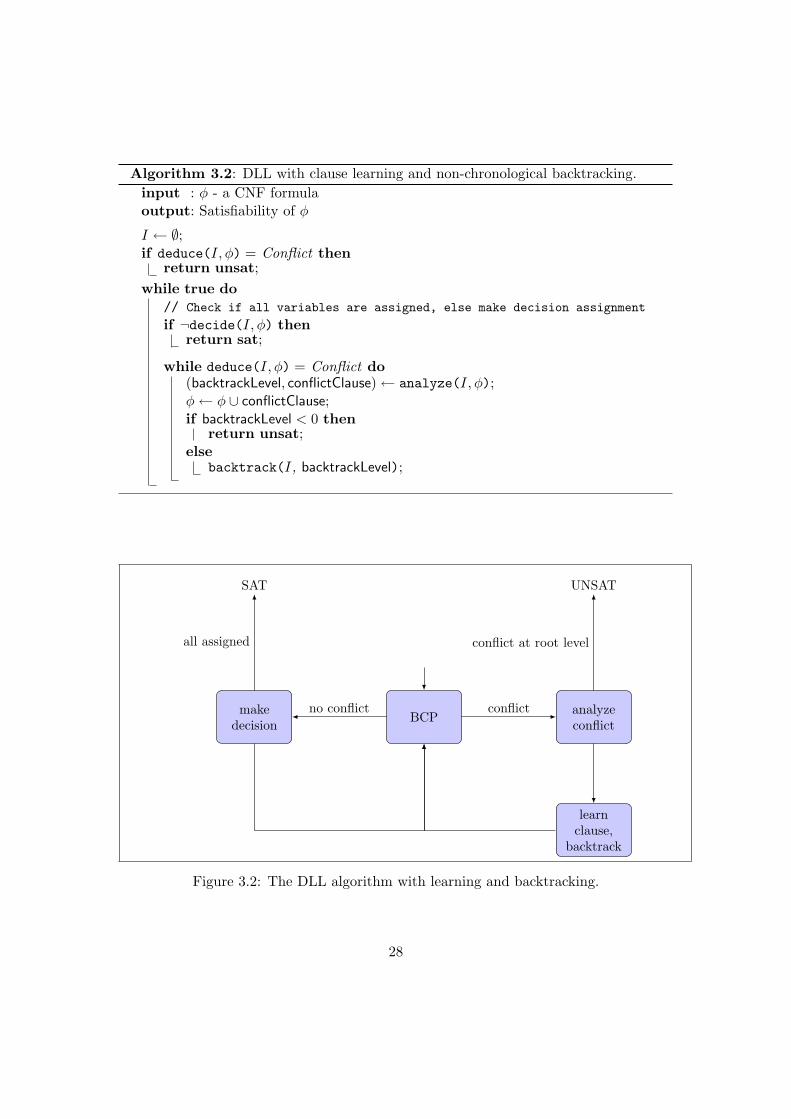
Above, an example of an implication graph at a conflict is shown. The chosen responsible assignment isindicated by the red area, the resulting conflict clause is cconfl = ¬v7 ∨ v1 ∨ v10.
Newer implementations of conflict-driven backtracking (red) differ slightly from Grasp’s originalbacktracking strategy [33] (green). Grasp backtracks to the highest decision level, newer solvers to thesecond-highest level.
......
...
dlevel 4 v4 := 0@4
v7 := 1@4
dlevel 5v2 := 1@5
v5 := 1@5v1 := 0@5
v10 := 1@5
......
...
dlevel 11
v10 := 1@11
Figure 3.1: Example for learning, non-chronological backtracking, and conflict-drivenassignments.
25

can generate other responsible assignments. This “replacement” is actually a resolutionstep, as was briefly described before, the variable resolved upon being the variable thatwas assigned a value due to BCP. For an example of a responsible assignment after aconflict, consider Figure 3.1.
We can then create a clause which acts as a constraint, ensuring that the sameset of assignments will not occur again. For the set of responsible assignments S, theadded conflict clause cS contains exactly those literals which are contradicted by theassignments in S, e.g., for S = {x1 := >, x2 := ⊥, x3 = >} we would have cS =¬x1 ∨ x2 ∨ ¬x3. The next time a similar region of the search space is encountered, theadded clause may act as an implication shortcut which may instantly force a variableassignment via BCP, where otherwise, the solver would have to resort to decisions todetermine the value of the variable.
3.2.2 Non-Chronological Backtracking
After a conflict has been identified, traditional implementations of the DLL procedurewould backtrack chronologically, i.e., they would reset the solver to the highest decisionlevel where both values of a decision variable have not been tried out. The solver wouldthen proceed the solving process by assigning to this variable the so far untried value.This technique is called chronological backtracking.
In non-chronological backtracking (also referred to as conflict directed backjumping),a solver may backtrack further than that, essentially leaving a number of branches unex-plored. The main idea is that in backtracking, a SAT solver can skip over all unexploredbranches which are sure not to lead to a satisfiable assignment. The identification ofthe backtracking level relies on the implication graph described above and is closelyconnected with the idea of learned clauses.
Non-chronological backtracking was not invented in SAT solving, but is a well studiedtechnique originating in the area of constraint satisfaction problems under the name of“dependency directed backtracking” [40].
When a conflict is encountered, a clause is learned by analyzing the conflict andidentifying a responsible assignment S from the implication graph. From this responsibleassignment, we can determine the maximal decision level associated with any individualassignment in S
dmax = max(v:=X)∈S
dLevel(v).
Since the learned clause is added to the instance, resulting in a logically equivalentinstance, the solver state will remain conflicting until at least one of the assignments inS is undone. Even if the learned clause is not added to the clause database, the solveris guaranteed to encounter only conflicts if we backtrack to any decision level d ≥ dmax
since the learned clause just provides a shortcut to an exploration of a certain part of thesearch space in the original instance. The unexplored branches from the current levelup to the start of dmax can safely be skipped.
Each of the skipped branches could theoretically unfold to a partial search tree that isexponential in the size of the remaining variables. Non-chronological backtracking can
26

result in considerable performance improvements because it prevents the solver fromentering or staying in such uninteresting regions of the search space.
We can also think of non-chronological backtracking as a way of recovering the solverfrom the negative consequences of bad decision orderings. In a good variable ordering,conflicts are produced as soon as possible, i.e., conflicting decisions are grouped closetogether. In the case of a bad ordering in the traditional DLL procedure, the variableassignments for a given conflict may occur on widely separated decision levels, whichmay lead to an exponential increase in runtime compared to a good ordering. Non-chronological backtracking can help to identify this wide level-span between conflictingvariables and jump back to the earlier levels sooner.
3.2.3 DLL with Clause Learning and Non-Chronological Backtracking
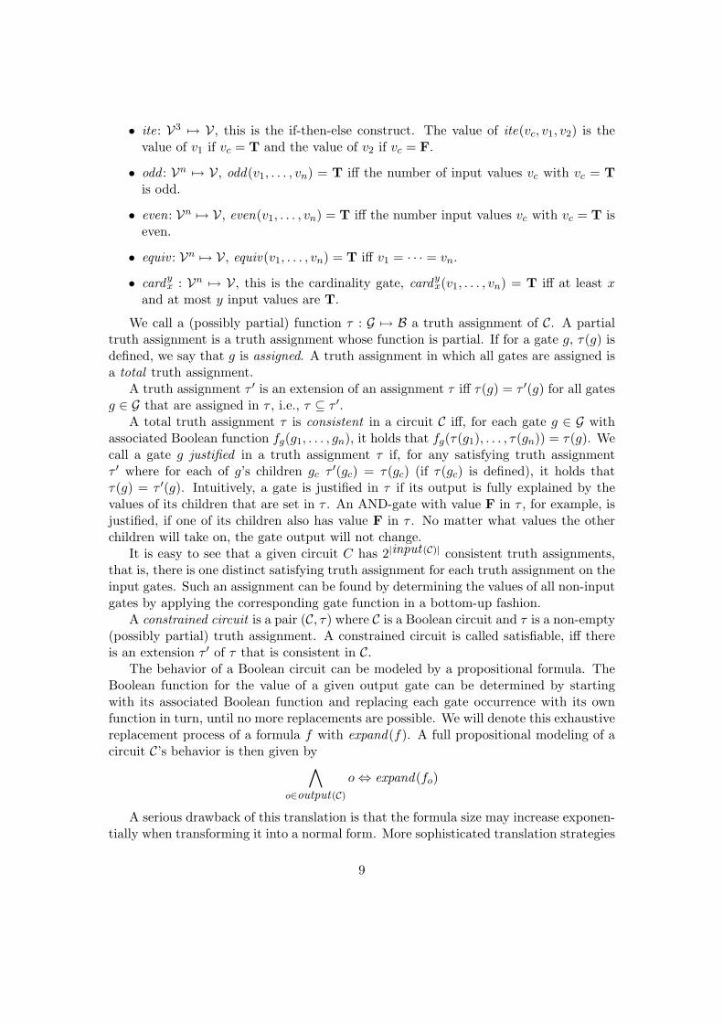
Since clause learning and non-chronological backtracking change the structure of the DLLprocedure considerably, it is useful to recharacterize DLL in the iterative formulationin Algorithm 3.2. The deduce function performs BCP and determines if a conflict hasoccurred, decide performs a decision assignment or returns false if no more decisionscan be made. The analyze function is called when a conflict has occurred. It adds aconflict clause to the clause database and determines a backtracking level. If it wouldbe necessary to undo assignments at decision level 0, that is, if the conflict does notdepend on any decisions made, the instance is unsatisfiable. Otherwise, backtracking isperformed and the newly learned clause is used in BCP to advance into new parts of thesearch space.
The code in Figure 3.2 is very close to how the DLL procedure is actually imple-mented. Since the structure of the algorithm is somewhat complex, a more abstract,graphical representation is also given in Figure 3.2.
3.2.4 Backtracking to the Second-Highest Decision Level
Grasp’s backtracking strategy is rather complex. There, the backtracking level is themost recent decision level found in the chosen responsible assignment. The first conflictof a decision always contains a literal of the most-recent decision level in any responsibleassignment. Therefore, Grasp always backtracks chronologically after the first conflictthat is encountered right after a decision. After this step, the first assignment thatis made is the result of a learned clause, i.e., its node in the implication graph hasantecedent vertices from earlier decision levels. If, at this point, a second conflict occurs,a responsible assignment can be found that contains only assignments made on earlierdecision levels (by traversing the implication graph backwards past the initial assignmentof the most recent decision level).
In contrast, modern solvers backtrack up to the second-highest decision level encoun-tered in the conflict clause that is, they backtrack as far as it is possible for the conflictclause to stay an asserting clause, i.e., a clause where all but one literal evaluate to falseunder the current partial assignment. The assignments made on the second-highest deci-sion level are not undone. Now, upon resuming BCP, the asserting clause becomes unit
27
Algorithm 3.2: DLL with clause learning and non-chronological backtracking.input : φ - a CNF formulaoutput: Satisfiability of φ
I ← ∅;if deduce(I, φ) = Conflict then
return unsat;while true do
// Check if all variables are assigned, else make decision assignment
if ¬decide(I, φ) thenreturn sat;
while deduce(I, φ) = Conflict do(backtrackLevel, conflictClause)← analyze(I, φ);φ← φ ∪ conflictClause;if backtrackLevel < 0 then
return unsat;else
backtrack(I, backtrackLevel);
BCP analyzeconflict
learnclause,
backtrack
makedecision
UNSATSAT
conflictno conflict
all assigned conflict at root level
Figure 3.2: The DLL algorithm with learning and backtracking.
28
and the resulting conflict-driven assignment takes the SAT solver into an unexploredregion of the search space. In Figure 3.1, an illustration of the two different approachesis presented via the implication graph.
The branches that are skipped between the highest and second-highest decision levelof the clause are not guaranteed to lead to conflicts. Essentially, part of the viable searchspace is thrown away and has to be explored again. The reasons for this counter-intuitivestrategy seem to be twofold, one systematic, the other technical in nature.
First, being able to deduce more at an earlier decision level may allow the solverto make heuristically smarter decisions on the direction of the search. The solver mayotherwise end up in a region of the search space which—while viable in the sense thata satisfying assignment may be found—it would not have chosen heuristically giventhe information learned in that region. Second, jumping back to the second-highestdecision level is easier to implement for a number of reasons. Together with the First-UIP clause-learning strategy (to be discussed in Section 3.3), it always produces assertingclauses. Also, in Grasp’s strategy, conflict clauses may be used in BCP only somesearch levels after they become eligible for BCP. Consider a responsible assignmentS = {v1 := 0@3, v2 := 1@4, v3 := 1@7}. Grasp would backtrack to decision level 7 andassign v3 := 0 via BCP, while, in fact, it could have already been assigned at decisionlevel 4. When subsequently backtracking to level 5, for example, care should be takenthat v3 := 0 is not undone along with the other assignments.
Ideally, a SAT solver will choose a clause learning strategy which produces conflictclauses that are asserting clauses. This has the advantage that upon backtracking, theconflict clause becomes a unit clause and causes the solver to enter another part of thesearch space. This new variable assignment is then called conflict-driven assignment.
Conflict-driven backtracking raises the issue of completeness. If parts of the viablesearch space are thrown away, can we be sure that the solver does not run into a cyclewhere a number of partial assignments are repeated? Indeed, we can; as long as thesolver produces only asserting clauses, we can prove that a solver can never run into apartial interpretation twice. First, we need to introduce some concepts that allow us toformalize parts of the DLL procedure:
For a SAT instance φ, we define the state of a DLL solver that follows the frameworkof Algorithm 3.2 as the number of times the deduce-function was called. A state S islater than a state S′ if S′ < S, and earlier if S < S′. The current partial interpretationfor a state S is denoted by I(S), the current decision level for a state is denoted bydLevel(S). A state S is non-conflicting if no clause is false under I(S).
Theorem 3.2.1. Given a DLL solver that follows the framework of Algorithm 3.2,produces only asserting conflict clauses, and backtracks to the second-highest decisionlevel of a responsible assignment. Then there can be no pair of distinct non-conflictingstates (S1, S2) where S2 is later than S1 and I(S1) = I(S2).
The following induction proof is based on the shorter proof given in Kroning andStrichman [27]. The main intuition is that whenever a solver backtracks, the search istaken to a fresh region of the search space through the conflict-driven assertion.
29

dLevel = 0
. . .
S−− (dl−−)
. . .
S− (dl−)
. . .
S1 (dl)
. . .
� (dl+)
. . .
�
. . .
S∗2
. . .
S2
Figure 3.3: An illustration of the induction step of the proof of Theorem 3.2.1.
Proof. Let S1 be a non-conflicting state at decision level dl. Assume furthermore, thatthere is another, later state S2 distinct from S1 where I(S1) = I(S2), which would be anecessary requirement for a cycle to occur.
If the solver is to proceed from S1 to S2, it must encounter a conflict at a decisionlevel dl+ > dl which causes the solver to backtrack to a state S− at a decision leveldl− ≤ dl.
We claim that, for any such pair of states (S1, S2) and any such decision level dl−,it holds that I(S2) 6⊆ I(S1) and therefore I(S1) 6= I(S2). We use induction over dl− toprove this.
First, take the case where dl− = 0. Let cdl+ be the conflict clause that was learned inthe conflict at dl+. Since, by assumption, cdl+ is an asserting clause, it is unit at decisionlevel 0 and produces a conflict-driven assignment (a := v) ∈ I(S−). The conflict-drivenassignment must be the opposite phase to an assignment a := v that was made on adecision level dl′ with dl < dl′ ≤ dl+. Therefore, it holds that (a := v) /∈ I(S1). SinceS− is at decision level 0, any interpretation I(S′) of a subsequent state S′ must be anextension of I(S−) and therefore contain (a := v). Since S2 is such a subsequent state,I(S2) must contain (a := v). Since (a := v) /∈ I(S1), it holds that I(S2) 6⊆ I(S1)
We can now formulate our induction hypothesis as follows:
30

For any pair of states (S1, S2) where S1 is earlier than S2 and the first backtrackafter S1 to a decision level smaller or equal than dLevel(S1) is to a level smaller thandl−, it holds that I(S2) 6⊆ I(S1).
It remains to show that I(S1) ⊆ I(S2) ⇒ I(S2) 6⊆ I(S1) if the first backtrack toa level smaller or equal than dLevel(S1) is to dl−. Let S− again be the state afterbacktracking and assume that S2 ≥ S−. We can distinguish two cases.
• S2 is reached from the original backtracking state S− without any further back-tracks to decision levels smaller or equal to d−.
Then we can reason analogously to the case dl− = 0 that I(S2) contains a conflict-driven assignment which is not contained in I(S1). Therefore, it holds that I(S2) 6⊆I(S1).
• At least one conflict is encountered between S− and S2 that causes a backtrack toa decision level smaller than dl−. Since this case is rather complex, an illustrationis given in Figure 3.3. Now let S−− be the latest state with S− < S−− < S2,where
∀S′ : S− < S′ < S2 ⇒ dLevel(S−−) ≤ dLevel(S′)
Thus, S−− is the state right after the last minimum-decision-level backtrack thatoccurs between S− and S2.
Now assume that I(S2) ⊆ I(S1). To reach S2 from S−− it is then first necessary toreach a state S∗2 where I(S∗2) ⊆ I(S−) (since I(S−) ⊆ I(S1). Therefore, (S−, S∗2) isa pair where S− is earlier than S∗2 and the first backtrack to a decision level smallerthan dLevelS− is to a decision level smaller than dl−. Furthermore, I(S∗2) ⊆I(S−).
This contradicts our induction hypothesis, therefore I(S1) 6⊆ I(S1), since we knowthat such a state S∗2 cannot be found after a backtrack to a decision level smallerthan dl−.
Therefore I(S1) 6= I(S2).
The introduction of conflict-driven assignments changes the structure of the searchprocess subtly. While in traditional DLL, both values of a variable have to be systemat-ically tried out, in DLL with learning and non-chronological backtracking, we only tryout one phase of a variable. If this assignments runs into a conflict, a clause is learnedthat takes the solver to a new part of the search space automatically after backtrack-ing by virtue of a conflict-driven assignment. All this is conveniently handled by thestandard BCP mechanism and needs no special implementation.
31

3.2.5 Clause-Database Management
A short overview of different clause-database implementations is given in Zhang andMalik [54]. In most cases, a sparse matrix representation is used to represent clauses,i.e., each clause is represented as an array of literals occurring in the clause. Literalsthemselves are usually represented as integers, an integer i representing the literal viand −i representing ¬vi. A common trick that is used in SAT solvers (e.g., MiniSAT) isto use the least significant bit to store the sign, since the variable can then be retrievedsimply by a right-shift instead of an “if” operation.
The early SAT solvers Grasp [33] and rel sat [2] used pointer heavy datastructures tostore clauses. This has disadvantages in cache-efficiency since the pointer dereferenceslead bad cache efficiency in BCP. Modern solvers usually store the clauses in a largelinear array, which necessitates dedicated garbage collection code, but is more efficientoverall. Zhang and Malik [54] report some techniques that use zero-suppressed binarydecision diagrams [9] or tries [52] to store clauses, but find that the additional overheadis not worth the performance increase. A possible advantage of more structured clausedatabase formats is an easy identification of duplicate and subsumed clauses (clauseswhose literals are a subset of another clause’s literals) for on-the-fly clause-databasesimplification.
Besides questions of implementation, systematic issues arise pertaining to the ques-tion of how to deal with the growth of the clause database which is exponential in thenumber of variables in the worst-case. In Grasp [33], a space-bounded diagnosis engineis proposed which makes this worst-case growth polynomial. First an integer k is cho-sen. Newly learned clauses that have more than k literals are marked for early deletion.They must be kept as long as they define conflict-driven assertions (in order to keep thesolver complete), but are deleted immediately afterwards. Since learned clauses encoderedundant information encoded in the original CNF instance, deleting clauses does notcompromise correctness.
The solver rel sat [2] proposes to delete clause of low relevance. A clause is consideredrelevant if few of its variables have changed assignment since the clause was derived. Theintuition is to find a way to identify clauses that have a low chance of being used to deriveconflicts or unit-assignments in the current part of the search space. BerkMin [19] uses acombined strategy of deleting old clauses with many literals that have not been involvedin conflicts recently. The age of a clause is implied by its position on the clause stack.For the clause activity, counters are associated with each clause which count the numberof conflicts the clause has helped derive. Counters are periodically divided by a constant,so that more recent activity has relatively higher impact than less recent activity.
3.3 Strategies for Clause Learning
Given a single conflict, there is a number of possible responsible assignments that canbe chosen to induce a conflict clause. A very simple strategy would be to choose asa responsible assignment all decisions that have been made so far. Obviously, this
32

assignment is sufficient to produce the conflict. The conflict clause induced by thisassignment is on the other hand not very useful. Exactly the same arrangement isunlikely to occur again very often during the search, therefore the clause will be unlikelyto be useful in pruning the search space.
There are some properties which seem useful when choosing a conflict clause, someof which are discussed in Zhang et al. [55]. First, the conflict clause should be smallsince small clauses are considered more powerful in pruning the search space on aver-age. Second, there may be advantages in choosing a responsible assignment as closeto the conflict as possible in the implication graph. Finally, the literals in the conflictclause should also have low decision levels, since this increases the gains from potentialbackjumps.
3.3.1 Unique Implication Points (UIP)
The idea of choosing strong implicants for learned clauses goes back to the seminal paperof Marques-Silva and Sakallah [33], the initial idea being to produce shorter clauses.The idea is illustrated in Figure 3.4. Instead of choosing both v2 := 1 and v1 := 0 fora responsible assignment, we could choose to include v0 := 0 since it is in some sense“stronger” as it implies both of the former assignments. We can formalize this notionby introducing the concept of domination. In an implication graph, a node x at leveld is dominated by a node y at the same level iff every path from the decision variableof level d to x goes through y. Therefore, in the above example, v3 := 1 dominates theconflict node, but v1 := 0 does not, since a path (v0 := 0, v2 := 0, v3 := 1,�) is possiblewhich does not include v1 := 0. Using the concept of domination, we can now give adefinition of unique implication points (UIPs).
Definition 15. A unique implication point is a node in the conflict graph that dominatesthe conflict node.
In this definition, only nodes that are on the most recent decision level can be UIPs.As an example, consider the implication graph in Figure 3.4 with two UIPs.
v0 := 0@2
v1 := 0@2
v2 := 1@2
v3 := 1@2
v5 := 1@1
� v4 := 0@0
UIPs
Figure 3.4: A simple implication graph with two unique implication points (UIP).
33

The idea of choosing a UIP as part of the responsible assignment is important sinceonly learned clauses that contain a UIP variable can be asserting clauses. The mostrecent decision is always a UIP, which raises the question why we would want to investthe effort into finding other UIPs at all. A possible answer to this question is that UIPswhich are closer to the conflict are, in some sense, more general since they encode themore immediate reasons for a conflict. Also, keeping UIPs close to the conflict reduces thenumber of assignments from earlier decision levels in the responsible assignment hencekeeping the overall clause size smaller. Biere [3] makes a very interesting observationon this: Beside the general heuristic gain by smaller clauses, the chances also rise thatthe second-highest decision level of the clause is earlier compared with a longer clause.This allows for longer backjumps after each conflict which may account for much of theperformance gain obtained by using UIPs close to the conflict node.
The concept of UIPs has been extended in Zhang et al. [55] to include nodes on earlierdecision levels in a way which depends on the chosen responsible assignment. For thedefinition, we will borrow the concept of a separating cut from Kroning and Strichman[27].
Definition 16. A separating cut in a conflict graph is a subset-minimal set of edgeswhose removal breaks all paths from the root nodes to the conflict node.
In Figure 3.4, examples for separating cuts are {v3 := 1, v4 := 0}, {v1 := 0, v2 :=1, v4 := 0}, or {v0 := 0, v5 := 1, v4 := 0}.
The assignments that make up a cut always constitute a responsible assignment forthe conflict. Given a cut, we can partition the conflict graph into a conflict side and areason side. The conflict side contains all nodes that are on a path from a node in theseparating cut to the conflict node. The reason side contains all other nodes. We cannow generalize the concept of unique implication points to multiple decision levels.
Definition 17. Given a separating cut T , a node x is a unique implication point atdecision level d iff any path from a root node either goes through x or through a node yon a decision level d′ > d, where y is on the reason side of the partition given by T .
Note that in the case of the most recent decision level, the two definitions are identi-cal, i.e., a UIP is always a UIP at the most recent decision level. We call a UIP u1 earlierthan another UIP u2 on the same decision level if u2 dominates u1. The first UIP isthe earliest UIP on the most recent decision level. The last UIP is the first assignment(usually the decision assignment) on the most recent decision level.
The concepts of last cut and first cut are defined in the following way.
Definition 18. Given an implication graph with a conflict, the first cut is the separatingcut that includes exactly the first UIP and those nodes on earlier decision levels that havean edge to the conflict side of the most recent decision level.
Definition 19. Given an implication graph with a conflict, the last cut is the separatingcut that includes exactly the last UIP and those nodes on earlier decision levels that havean edge to the conflict side of the most recent decision level.
34

3.3.2 Choosing a Cut for a Learned Clause
At each conflict, it is possible to learn a number of clauses that encode reasons for theconflict. Each separating cut on the implication graph yields a distinct learned clause.In Zhang et al. [55], detailed descriptions and comparisons of different learning strategiesare given. The following information about Grasp’s and rel sat’s learning strategies willbe taken from there, since a more in-depth description is given than in the originalpapers.
The two first solvers that included learning and backtracking, rel sat [2] and Grasp[33], have very different clause learning strategies. The solver rel sat simply adds theconflict clause that is induced by the last cut. The responsible assignment thus includesthe decision variable of the most recent decision level and all assignments from earlierlevels that have an outgoing edge to a node on the conflict side. Grasp’s [33] strategyis described in detail in Zhang et al. [55]. It is unique for two reasons. First, differentclause learning strategies are used in the solver depending on the current status of thesearch where in each multiple clauses are learned for one conflict. Second, some clausesthat are learned do not result from conflicts, but constitute general deduction shortcuts.Grasp uses two solver modes that determine how learning is done.
The first, referred to from now on as “decision mode”, is active whenever a conflict isencountered as a direct result of a decision. The second, “backtracking mode”, is activewhenever the solver encounters a conflict when the first assignment on the conflictingdecision level was made due to a result of an earlier conflict. Some of this complexitymay arise from the fact that Grasp chooses the highest decision level encountered ina conflict clause as a backtracking level instead of the second-highest. Therefore thefirst assignment made on a decision level may itself be implied by assignments made onearlier decision levels, i.e., the first assignment on a decision level may have antecedentsin the implication graph.
Grasp follows the strategy of learning more than one clause from each conflict. In de-cision mode, the first-cut scheme is used to induce a conflict clause. Additionally, clausesare learned which encode deduction shortcuts for UIPs. In backtracking mode, the sameclauses are learned as in decision mode with the addition of a so-called back-clause. Theback-clause contains only assignments made on earlier decision levels. It can be foundby tracing back the implication graph from the conflict node until assignments on earlierdecision levels are encountered. This corresponds to the cut where all assignments onthe most recent decision level which are on a path to the conflict are on the conflict sideand all other assignments on the reason side. After learning the back-clause, the solverbacktracks to the highest decision level of any assignment in this cut.
The first-cut scheme that is used in Grasp can also be extended to multiple decisionlevels using our generalized definition of a UIP. For this, we first determine the parti-tioning of assignments on the most recent decision level according to the first cut. Thenwe can step up one decision level and identify a UIP at this earlier level using the partialpartitioning on the more recent level below. This can be repeated for an arbitrary num-ber of decision levels. While this seems intuitively useful since it reduces the size of thelearned clause, Zhang et al. [55] conclude in an in-depth analysis of learning strategies
35

that the most efficient overall strategy seems to be to just learn one clause correspondingto the first cut, and not try to find UIPs at earlier levels. This strategy also performedbetter than the Grasp and rel sat learning schemes. Biere [3] suggests that this increasemay result from the increased locality of the search. The first-cut scheme is also themost commonly used learning scheme in newer solvers (e.g, MiniSAT, RSAT).
3.4 Efficient Datastructures for BCP
In DLL algorithms, Boolean Constraint Propagation (BCP),i.e., the exhaustive applica-tion of the unit rule, is usually by far the most time consuming subtask. It is estimatedthat BCP takes up about 90% of the runtime in a typical solver [34]. Therefore, im-proving the efficiency of this step is one of the most crucial aspects in engineering a fastimplementation.
One of the main determining factors for the efficiency of any implementation is thechoice of datastructures. In BCP, the areas of special interest are those which areinvolved in determining the state of a clause at any point in the search process, thatis, to determine when a clause becomes unit, conflicting, or satisfied under the currentpartial assignment. Newer SAT solvers do usually not distinguish between clauses thatare satisfied and unresolved clauses. The additional overhead of managing such a clauselist is not worth the benefits.
We can broadly distinguish between busy and lazy datastructures for determiningthe state of a clause. Busy datastructures update the state of a clause immediately afterone of its literals has been assigned. Early SAT solvers such as GRASP [33] used thisapproach. A major performance improvement was obtained by using lazy datastructures.They perform more work at each state update, but such updates are not performed everytime a clause literal is assigned. Compressing more related work into steps that happenless often increases space locality. Clause literals are usually stored in contiguous blocksof memory. Accessing more than one literal at each state update therefore accesses thecache instead of the main memory, which leads to an overall performance improvement.
The average numbers of accesses per variable assignment that are presented in thefollowing discussion are taken from [53].
3.4.1 Counter-Based Approaches
Most prominent in the category of busy datastructures is the counter-based approach,in which literal assignments are represented by counters associated with each clause.In Zhang and Malik [53], the first use of this approach is traced back to Crawford andAuton [11]. Clause counters are updated when a variable is assigned, and have to beundone during backtracking.
Grasp [33] uses a simple version of the counter-based approach, counting the numberof satisfied (cs) and unsatisfied (cu) literals for each clause, and checking these valuesagainst the total number of literals nl in the clause. Unit clauses and conflict clausescan then be efficiently determined.
36
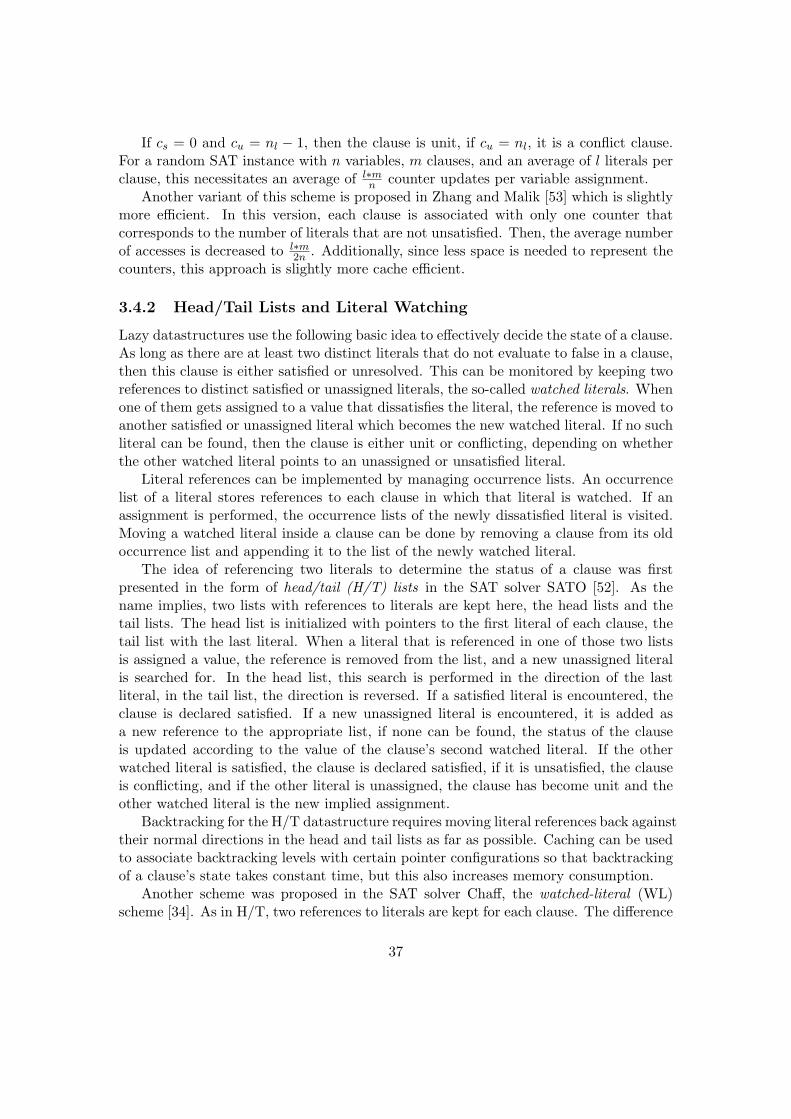
If cs = 0 and cu = nl − 1, then the clause is unit, if cu = nl, it is a conflict clause.For a random SAT instance with n variables, m clauses, and an average of l literals perclause, this necessitates an average of l∗m
n counter updates per variable assignment.Another variant of this scheme is proposed in Zhang and Malik [53] which is slightly
more efficient. In this version, each clause is associated with only one counter thatcorresponds to the number of literals that are not unsatisfied. Then, the average numberof accesses is decreased to l∗m
2n . Additionally, since less space is needed to represent thecounters, this approach is slightly more cache efficient.
3.4.2 Head/Tail Lists and Literal Watching
Lazy datastructures use the following basic idea to effectively decide the state of a clause.As long as there are at least two distinct literals that do not evaluate to false in a clause,then this clause is either satisfied or unresolved. This can be monitored by keeping tworeferences to distinct satisfied or unassigned literals, the so-called watched literals. Whenone of them gets assigned to a value that dissatisfies the literal, the reference is moved toanother satisfied or unassigned literal which becomes the new watched literal. If no suchliteral can be found, then the clause is either unit or conflicting, depending on whetherthe other watched literal points to an unassigned or unsatisfied literal.
Literal references can be implemented by managing occurrence lists. An occurrencelist of a literal stores references to each clause in which that literal is watched. If anassignment is performed, the occurrence lists of the newly dissatisfied literal is visited.Moving a watched literal inside a clause can be done by removing a clause from its oldoccurrence list and appending it to the list of the newly watched literal.
The idea of referencing two literals to determine the status of a clause was firstpresented in the form of head/tail (H/T) lists in the SAT solver SATO [52]. As thename implies, two lists with references to literals are kept here, the head lists and thetail lists. The head list is initialized with pointers to the first literal of each clause, thetail list with the last literal. When a literal that is referenced in one of those two listsis assigned a value, the reference is removed from the list, and a new unassigned literalis searched for. In the head list, this search is performed in the direction of the lastliteral, in the tail list, the direction is reversed. If a satisfied literal is encountered, theclause is declared satisfied. If a new unassigned literal is encountered, it is added asa new reference to the appropriate list, if none can be found, the status of the clauseis updated according to the value of the clause’s second watched literal. If the otherwatched literal is satisfied, the clause is declared satisfied, if it is unsatisfied, the clauseis conflicting, and if the other literal is unassigned, the clause has become unit and theother watched literal is the new implied assignment.
Backtracking for the H/T datastructure requires moving literal references back againsttheir normal directions in the head and tail lists as far as possible. Caching can be usedto associate backtracking levels with certain pointer configurations so that backtrackingof a clause’s state takes constant time, but this also increases memory consumption.
Another scheme was proposed in the SAT solver Chaff, the watched-literal (WL)scheme [34]. As in H/T, two references to literals are kept for each clause. The difference
37

Watched literals:
¬v1 v2 v3 ¬v4
Head/tail literals:
¬v1 v2 v3 ¬v4
v4 := 1
¬v1 v2 v3 ¬v4 ¬v1 v2 v3 ¬v4
v1 := 1
¬v1 v2 v3 ¬v4 ¬v1 v2 v3 ¬v4
v3 := 0
¬v1 v2 v3 ¬v4 ¬v1 v2 v3 ¬v4
no free literal ⇒ UNIT
backtrack v1, v2, v3, v4
¬v1 v2 v3 ¬v4 ¬v1 v2 v3 ¬v4
Consider the example clause¬v1 ∨ v2 ∨ v3 ∨ ¬v4
above and its state changes during BCP. In the watched-literal (WL) scheme (left), thewatch pointer movement direction can be arbitrary. In the head/tail-list (H/T)scheme, the head literal always moves left-to-right, and the tail literal right-to-left.
During backtracking, no work needs to be done for WL. For H/T, the head and tailpointer have to be moved to the leftmost and rightmost non-conflicting literalrespectively.
Figure 3.5: Chaff’s watched literals and SATO’s head/tail lists.
38

between the two schemes is that in WL, no special order or search direction is imposedon the literals. The only requirement when searching for a new position is that the newliteral is unassigned or satisfied.
This may lead to more time being spent in search for a new unassigned literal when-ever a clause’s status is updated, but this is a operation that is highly local in memoryand therefore very cache efficient. Another advantage of WL is that it removes the needfor changing any clause’s references during backtracking.
To summarize, the watched-literal scheme as implemented in Chaff [34] performs thefollowing steps when processing an assignment to an opposite-phase watched literal:
Step 1 Search for a new unassigned or satisfied literal.
Step 2 If such a literal exists and it is not the second watched literal of the clause, movethe watched literal to the new position by removing the clause reference from theold watch list and appending it to the watch list of the new watched literal.
Step 3 If no such literal exists, check the status of the other watched literal:
3.1 If the other watched literal is unassigned, the clause is unit.
3.2 If the other watched literal is unsatisfied, the clause is conflicting.
In a SAT solver that uses the WL scheme, performing the above steps usually takesup most of the runtime. It is therefore worthwhile to investigate highly efficient im-plementations as is done in Biere [5]. A popular approach used in many solvers is toassociate each literal with a list (or stack) of so-called watcher datastructures. Thesewatchers keep a reference to a clause and its watched literals. Biere [5] proposes insteadto reference the clause as a whole and keep the watched literals at the first and secondposition of the clause respectively. This avoids the overhead of separate watcher data-structures and yields an improved cache efficiency. Figure 3.6 illustrates this technique.
3.4.3 Special Handling of Small Clauses
In many practical problem instances, binary and ternary clauses, i.e., clauses with twoor three literals take up a considerable percentage of the input instance. Given a randomvariable assignment, the chance of such a clause becoming unit is relatively high. Unit-rule applications over binary clauses therefore may make up a considerable percentageof BCP.
For binary clauses, determining their status with the standard WL technique entailsconsiderable overhead compared with a more direct implementation. One possibilitywould be to add vectors of direct implications, which—similar to the implication graphin 2-CNF—store for every literal l all other literals l′ where l∨ l′ is a binary clause in theclause database. Whenever a variable is assigned a value, all resulting assignments dueto binary clauses can then be processed immediately. If one of the resulting assignmentsis impossible since the opposite value is already assigned to the destination variable, aconflict can be concluded.
39

Dedicated watcher:
Occurrence lists
¬v1
¬v2
¬v3
...
· · ·
· · · ¬v7 v3 v10 ¬v1 ¬v15
Watcher
v1
v2
v3
...
...
...
...
Watched literals at constant position:
Occurrence lists
¬v1
¬v2
¬v3
...
· · ·
· · ·
v10v3 ¬v1 ¬v7 ¬v15v1
v2
v3
...
...
...
...
Figure 3.6: Different implementations of the watched-literal scheme.
40

In the SAT solver FUNEX, clauses are divided into three classes (binary, small, andlarge), and only large clauses use the watched literal scheme (for a detailed discussion seeBiere [3]). MiniSat [39] uses mixed watch lists for literals, that contain both referencesto clauses and directly implicated literals from binary clauses. The reason given for thisimplementation choice is that, if stored separately, all direct implications are performedtogether either before or after the watched-literal BCP step, which is reported to leadto slightly less useful conflict clauses. On the other hand, the SAT solvers FUNEX andNanoSAT make use of implication lists exactly for this reason, i.e., to be able to processbinary clause implications before the actual BCP step. The reason given here is thatthe binary BCP step is less expensive and should therefore be used exhaustively beforegoing on to the more expensive watched-literal BCP step.
3.5 Variable Selection Heuristics
The DLL procedure is highly sensitive to the choice of decision variables. For satisfiableinstances, an optimal decision heuristic would be able to produce a result in a linearnumber of DLL steps by incrementally choosing decision variables from a satisfyingassignment. Of course, since SAT is NP complete, the problem to find any such perfectheuristic for an input formula must be NP complete itself, thereby moving the complexityof SAT into the decision heuristic. While such a perfect heuristic is not practicallyinteresting, it is still possible to find heuristics that work well in the average case forcertain classes of problems.
For unsatisfiable instances, a good decision heuristic would choose variables thatare expected to lead to conflicts as early as possible. This keeps the search tree fromexpanding unnecessarily by closing down unfruitful parts of the search space early inthe search process. Additionally, causing conflicts early produces short conflict clauses.Short conflict clauses are more powerful than long conflict clauses since they prunelarger parts of the search space. In many SAT implementations, long learned clausesare removed from the clause database after a while or not even stored for exactly thisreason.
Another important consideration when choosing a decision heuristic is its efficiency.Often a trade-off has to be considered between the predictive power of a heuristic andthe runtime that is consumed by its computation.
3.5.1 Early Heuristics
Early decision heuristics were usually greedy in the sense that they tried to maximizethe number of implications that a given variable assignment would produce. In orderto estimate the consequences of a variable assignment, some heuristic function over theinput CNF-formula and the current partial assignment is used. Examples are Bohm’sheuristic and the Maximum Occurrences on clauses of Minimum size heuristic (MOM),both of which are briefly described in Marques-Silva [32]. Both of these choose literalswhich satisfy the highest number of possible clauses considering only unsatisfied clauses
41

of minimum length. Moreover, both try to choose a balanced variable, for which bothliterals fulfill this criterion to some extent. They differ in the exact balancing methodthat is used. Bohm’s heuristic just calculates a linear weighting of both literals’ scoresfor a variable, whereas MOM uses a non-linear function.
Dynamic largest independent sum (DLIS), originally presented in Marques-Silva [32],is a conceptually simpler, but nevertheless effective heuristic based on counting liter-als. Here, the decision assignment is chosen that makes the literal with the highestindependent occurrence count among unsatisfied clauses evaluate to true. The term“independent”, here, refers to the fact that the score of the opposite-phase literal doesnot influence the decision, i.e., for choosing a phase, DLIS is a greedy heuristic, not abalanced one.
3.5.2 Second-Order Heuristics
While earlier decision heuristics were functions of the current state of the solver, theSAT solver Chaff [34] introduced second-order heuristics that are functions not only ofthe current, but also of the preceding states of the solver.
Specifically, a second-order heuristic called Variable State Independent Decaying Sum(VSIDS) was introduced, which depends closely on the conflict analysis step that Chaffuses for clause learning and non-chronological backtracking.
VSIDS essentially estimates a literal’s likelihood to produce conflicts by pushing asliding window over all literals involved in recent conflicts. Each literal on the variables inthe input formula is associated with two counters that are initialized to zero. Whenevera conflict is encountered, the counters for the literals occurring in the conflict clause areincreased. In the decision step, a branching literal with maximum score is chosen forassignment. Periodically, all counters are divided by a constant. This leads to olderconflicts becoming less relevant for a literal’s score, which, in turn, increases the localityof the search.
In the SAT solver BerkMin [19], a number of changes are made to the VSIDS pro-cedure. The most important change is that the choice of a decision literal, while still ingeneral guided by the maximum score, is confined to the so-called top clause. The topclause is the most recently learned clause that is not satisfied.
The idea behind this procedure is to increase the mobility of the search, that is, toincrease the speed at which the search refocuses on a new part of the search space. Ifthe search enters a new region, e.g., by backtracking non-chronologically, VSIDS maymake bad decisions for a number of iterations due to the fact that its literal scoreschange only slowly to reflect the circumstances of the new part of the search space.BerkMin’s strategy of choosing a literal of the top-clause as decision variable reducesthis lag considerably by further promoting variables involved in recent conflicts. A naiveimplementation can lead to a large percentage of the runtime being spent searching forthe top clause. Caching of the location of the top clause in the clause stack eliminatesthis problem.
Another change to VSIDS is that, in BerkMin, instead of just incrementing the scoresof the conflict clause’s literals, the solver steps backwards through the implication graph
42

and increases literal scores of clauses that were involved in producing the conflict. If acertain literal occurs multiple times in the clauses, its score is also increased more thanonce. This entails a slightly higher overhead for the decision heuristic, but allows formore finely-grained estimation of a literal’s tendency to lead to conflicts.
3.6 Restarting and Randomizing the Search
As has been mentioned before, DLL-based SAT procedures are highly sensitive to thechoice of decision variables. Good variable orderings may yield exponential speed-upsin overall solving time compared to bad ones, but the computation of such orderings isa hard problem in itself. Usually, some kind of heuristic is used to prevent the solverfrom entering fruitless regions of the search space, but these are far from infallible. Theproblem is mitigated somewhat by non-chronological backtracking and learning, whichprune large parts of the search space, but the problem still remains. Biere [5] notes thatthis is especially a problem in industrial instances, since they are mostly either easy torefute or easy to prove, given the right variable ordering.
In Gomes et al. [20], this behaviour is referred to as a “heavy-tailed cost distribution”since there is a non-negligible chance that a variable ordering will lead to very long run-times. They argue for introducing random restarts into combinatorial search algorithmsin order to increase overall robustness by increasing the chances that a “good” searchpath will be chosen. In this technique, some transient randomness is introduced into thesearch process and the search procedure is reset at some points. Random restarts wereimplemented in Chaff [34] and are a feature of most competitive DLL SAT solvers sincethen. They form an especially effective combination with SAT solvers since informationcan be retained in between runs through learned clauses which implicitly encode partsof the visited search space in the clause database. In order to retain completeness, asolver must perform successively longer runs since, in the worst-case, the search spacewill have to be fully explored.
Introducing randomness into the decision heuristic can prevent the DLL procedurefrom being trapped in fruitless regions of the search space, and it allows for a broaderexploration of the same. This, in turn, allows decision heuristics to work more effectively.A similar argument was presented as to why “throwing away” parts of the search spacein backtracking seems to improve solving efficiency.
In Goldberg and Novikov [19], the authors of the solver BerkMin raise the issue ofclause-database symmetrization. They argue that restarts introduce asymmetry into theclause database since many variables may not be tried out in both phases, but just inone before a restart is triggered. If the decision heuristic does not account for restarts, itis possible for the solver to enter the same phase for these decision variables again. Thisleads to a situation where some variables mostly occur in one phase in learned clauses.For phase selection, Goldberg and Novikov [19] propose a modified strategy, where thedecision variable is chosen according to the VSIDS scheme among the top-clause literals,but not its phase. Counters are associated with each literal which count its occurrencein conflict clauses, and the phase is chosen that occurs more frequently in the clause
43

database. If this assignment leads to a conflict the opposite phase literal may be learnedin a clause thereby symmetrizing the database.
Another important question when using restarts is the restart schedule that is used.Usually, a restart is triggered after a fixed number of conflicts. This limit increaseswith every restart in order to guarantee the SAT solver’s completeness. Some work hasbeen done on trying to determine good restart policies. Earlier restart-limit sequenceswere usually strictly monotonically rising. MiniSAT [39], for example, uses a geometricprogression that starts with a clause limit of 100 and increases by a factor of 1.5 aftereach restart.
More recent solvers such as RSAT 2.0 [36] or PicoSAT [5] use restart-limit sequencesthat do not continually grow, but return to smaller restart-limits at times. In RSAT, therestarting limit sequence is based on the Luby sequence, which gives an optimal speed-upfor Las Vegas algorithms [31]. PicoSAT uses a similar scheme which uses two limits, aninner limit and an outer limit. The solver triggers restarts upon reaching the inner limitwhich is increased geometrically. When the inner limit reaches the outer limit, the innerlimit is reset to an initial value and the outer limit is increased. As can be seen in Figure3.7, PicoSAT’s strategy concentrates on very short restart intervals that only rise slowlyglobally, while RSAT’s strategy intersperses very long runs with very short ones.
Another interesting technique that works in combination with restarts is phase saving[35]. Phase saving means that upon backtracking or restarts, the phase of each assignedvariable that is undone is saved in an array. The next time a decision is made on ofthese variables, the phase indicated by the array is used first. If no array entry existsfor a variable, the default phase-selection heuristic is chosen. The motivation is thatthe solver may discard regions of the search space in non-chronological backtracking andduring restart which already encode satisfiable assignments for subproblems.
After backtracking or restarting, when the solver decides upon variables of the dis-carded search space, it automatically reenters parts of the search space similar to theone that was discarded. Biere [5] argues that phase saving “turbo charges” restarts. Thesolver immediately reenters regions of the search space that it left due to the restart andthus continues the search from where it left off.
3.7 Simplifying CNF formulas
Smaller CNF input formulas tend to produce shorter run-times for most SAT solvers.This relationship is, of course, not true in general. The idea of clause learning, forexample, is based on enriching the input formula with redundant clauses to speed upthe solving process. There are very small problems that are hard for SAT solvers as wellas large problems that are very easy. Still, it is useful to concentrate on the size of aformula since it is easy to determine and gives some estimation of SAT solver runningtime. Simplification can be used to replace the original formula with an equisatisfiableformula that is smaller in the number of clauses or variables in order to keep the runtimeof a SAT solver heuristically low.
44

0
100000
200000
300000
400000
500000
600000
0 2e+06 4e+06 6e+06 8e+06 1e+07 1.2e+07
RSAT 2.0PicoSAT
Figure 3.7: Comparing PicoSAT’s and RSAT’s restarting schemes. The x-axis showsthe number of conflicts, the y-axis shows the restart-limit.
45

3.7.1 Preprocessing SAT Instances
Many efficient preprocessing steps may be performed before the problem is actuallytranslated into a SAT instance given in CNF. These may include domain-specific simpli-fication techniques, efficient translation techniques into propositional form, and reduc-tion techniques that work on structured formulas, such as the identification of equivalentsub-formulas. Other techniques directly work on the resulting CNF and may be used inaddition with other prior reduction techniques. We will concentrate only on the latterin this section.
Some CNF preprocessing steps trace back to deduction rules in the original DP [12]procedure. One is the application of the pure literal rule, i.e., the removal of all clausesthat contain a literal occurring only in one phase in the CNF, which can be applied as alight-weight preprocessing step. The other is the application of the elimination rule foratomic formulas, reintroduced as a preprocessing step in the ZBDD-based SAT solverZRes [9], the quantified Boolean formula procedure (QBF) Quantor [6], and the dedicatedCNF preprocessor Niver [42]. Here, a variable is chosen, and the clauses containing thatvariable are replaced by their resolvents in the original instance. In general, this stepdoes not reduce size of the formula, it may, on the contrary, increase it exponentially.But if care is taken in the selection of variables resolved upon, the size of the formulacan be decreased and variables removed in the same step. Used as a preprocessing step,the elimination rule is referred to as clause distribution.
For both of these techniques, the integration into the main solving step has provedto be too expensive in modern implementations, but as preprocessing steps, they areefficient and light-weight ways of eliminating variables and clauses from formulas. Pre-processing is always a trade-off between the time spent in preprocessing and the expectedbenefits of running a SAT solver on the simplified formula. In Een and Biere [15], threeless trivial preprocessing techniques and efficient implementations are described, all ofwhich are included in the dedicated SAT preprocessor SatELite: Removal of subsumedclauses, strengthening clauses by self-subsuming resolution, and variable eliminations bysubstitution.
The authors note that clause distribution produces many subsumed clauses. Letlit(c) be the set of literals of a clause c, then a clause c1 subsumes another clausec2 if lit(c1) ⊂ lit(c2). Of course, subsumed clauses are not only an artifact of clausedistribution, but can occur naturally as part of the encoding of a problem. Since c1 willbe in conflict whenever c2 is in conflict, and c1 will be unit whenever c2 is unit otherwise,the addition of c2 in a SAT instance containing c1 does neither change the satisfiabilityof the the original formula nor add useful deduction shortcuts. The only significant wayin which c2 could influence the solving process is by influencing the decision heuristics insome way. Clauses that are subsumed can thus be removed from the instance, producingan equivalent instance with less clauses that is easier to solve.
In self-subsuming resolution, pairs of clauses are identified where one is almost sub-sumed by the other, except for a literal that occurs in opposite phases in both clauses.
Definition 20. Let c and c′ be clauses and x a propositional variable. Remember, that
46

⊗ is the binary resolution operator for clauses. The clause c is self-subsumed by c′ w.r. t. x iff lit(c⊗x c′) ⊂ lit(c).
Clauses that are self-subsumed by another clause w. r. t. to a variable x, can bereplaced in the instance with their resolvents over x. As an example, consider c1 =¬a∨b∨x and c2 = ¬a∨¬x. The resolvent of both clauses would be cr = c1⊗xc2 = ¬a∨b,which subsumes c1. Therefore, c1 can be replaced by cr in the SAT instance, effectivelyremoving a literal from the original clause.
The last technique presented in Een and Biere [15], the variable eliminations bysubstitution rule is motivated by the fact that many SAT instances are encoded viathe structure-preserving Tseitin transformation [47], which will be discussed in detailin Chapter 4. The Tseitin transformation is used to transform arbitrary propositionalformulas or circuits into equisatisfiable CNF-formulas by introducing new variables forsubformulas or gates. As an example, consider the simple formula
(x ∨ ¬y ∨ (u ∧ ¬v)).
A possible application of the Tseitin transformation would introduce a new variablez for the subformula (u ∧ ¬v) and produce the equisatisfiable formula
(x ∨ ¬y ∨ z) ∧ (z ⇔ (u ∧ ¬v))
which is subsequently transformed into the CNF
(x ∨ ¬y ∨ z) ∧ (¬z ∨ u) ∧ (¬z ∨ ¬v) ∧ (z ∨ ¬u ∨ v)
The newly introduced variables are functionally fully dependent on the variables oc-curring in the subformulas they name. If a naming variable such as x is removed in aclause distribution step, the effects of this renaming process are partially undone. Thisintroduction and subsequent removal of variables introduces some redundant clauses.The variable elimination by substitution rule directly tries to reconstruct gate definitionsused by the Tseitin transformation. If the preprocessor decides to remove a naming vari-able v of such a definition, instead of using clause distribution, the Tseitin transformationis locally undone by replacing all clauses containing v with the resolvents between thegate definitions and all other clauses where the naming variable occurs. Note that thisis just a subset of all possible resolutions on that variable. Een and Biere [15] prove thatrestricting the resolutions in this way yields a formula that is equivalent to the result ofperforming clause distribution on v and thus equisatisfiable to the original instance.
In the above example, the clauses that define the subformula {(¬z∨u), (¬z∨¬v), (z∨¬u∨ v)} would be resolved with the remaining clause {(x∨¬y∨ z)} in order to producethe formula
(x ∨ ¬y ∨ u) ∧ (x ∨ ¬y ∨ ¬v),
which would have been the result of directly translating the original formula into CNF.Directly using clause distribution, would have produced the CNF
(x ∨ ¬y ∨ u) ∧ (x ∨ ¬y ∨ ¬v) ∧ (u ∨ ¬u ∨ ¬v) ∧ (v ∨ ¬u ∨ ¬v).
47

In this case, it is easy to just check the newly produced distributed clauses for validityand thus remove the redundant clauses (u ∨ ¬u ∨ ¬v) and (v ∨ ¬u ∨ ¬v). In morecomplex examples, clause distribution can produce clauses which are not valid, but arestill redundant.
Note that the combination of the Tseitin transformation and subsequent variableelimination by substitution is functionally similar to approaches such as Boy de la Tour[8], where a translation procedure is presented that only introduces naming variablesif the introduction reduces the overall number of clauses. The variable elimination bysubstitution rule is more general in the sense that it can work on any given instance inCNF, no matter how it was translated.
Preprocessing as a means of speeding up the search process has proven to be a highlyeffective technique. The combination of the dedicated preprocessor SatELite with anefficient SAT solver has won the SAT 2005 competition on industrial benchmarks [43],and preprocessing has since been integrated into some of the fastest state-of-the-artsolvers, such as new versions of MiniSAT [16] and PicoSAT [5].
3.7.2 On-the-fly Clause-Database Simplifications
The techniques presented here are not only useful before the search process is started, butcan be applied during the search. Most prominently, if a solver uses a restarting scheme,a simplification step can be performed at each restart. This has been implemented withgood results in MiniSat 2.0 [16]. Moreover, earlier versions of the same solver alreadyintroduced another form of on-the-fly simplification: conflict-clause minimization.
In conflict-clause minimization, the self-subsuming resolution rule is invoked when-ever a conflict clause c is learned. Recall that each of the literals l in c corresponds toan opposite-phase assignment of the same variable in the conflicting implication graph.Each of these assignments, in turn, is associated with a clause c′ containing l that in-duced the assignment via the unit rule. Since c and c′ contain an opposite-phase literal,c is a candidate for being self-subsumed under c′.
Self-subsumption can be checked easily with the algorithm shown in Figure 3.3. Inessence, each literal in a newly learned clause is checked for possible removal under theself-subsumption rule. Intuitively, a clause that encodes the reasons for an assignmentdoes not need to encode that assignment itself.
Algorithm 3.3: MiniSAT’s on-the-fly clause minimization.input : A clause coutput: A possibly reduced clause c′
for each literal p ∈ c doif lits(reason(p)) \{p} ⊆ lits(c) then
mark(p);
c′ ← removeMarked(c);return c′;
48

Another application area for clause-database simplification is in incremental SATproblems. In incremental SAT, a series of closely-related SAT instances are solved oneafter another. An example of this are BMC runs with an increasing depth-bound k.Before each run, a formula is created that represents the formula of the last run, expandedby a new instance of the sequential circuit. A short study of applying simplificationsbetween runs of an incremental SAT solver can be found in Een and Biere [15].
49

Chapter 4
Solving SAT in Circuits
Many applications of SAT solving feature problems formulated as constrained Booleancircuits, i.e., circuits with some signals set to a fixed value. In order to solve theseproblems with traditional SAT solvers, they must first be translated into propositionalform, and then flattened into CNF, which yields an exponential increase in formula sizein the worst case. This problem of exponential growth can be sidestepped by solving thesatisfiability instance not on the original propositional formula, but on a satisfiability-equivalent formula with additional variables introduced for gates. Although some struc-tural information is still encoded in the resulting CNF, CNF-based solvers usually donot make use of this information.
This is a problem since the structural information could be used to speed up thesolving process. One possible approach is to use circuit information in order to changethe circuit-to-CNF translation, either by producing a smaller translation or by encodingadditional knowledge about the circuit structure into the CNF. Another possibility isto forego the use of a purely CNF-based solver altogether and explicitly work withstructural information in the solving process. Intuitively, we expect that the addedstructural information should lead to better heuristics, simplification techniques, andsearch strategies. On the other hand, the structurally simple format of CNF allows forhighly efficient implementation techniques and low-level optimizations, and given themore complex format of a Boolean circuit, it may be harder to achieve the same level ofefficiency.
This chapter aims to describe methods which try to speed up CNF-based solversby using sophisticated translation techniques as well as methods which directly usecircuit information in the solving process. Section 4.1 describes approaches which aimto improve the efficiency of circuit-to-CNF translations for use with traditional CNF-based SAT solvers. Section 4.2 deals with hybrid approaches, which combine CNF andcircuit representations, typically by enhancing a traditional SAT-Solver with circuit-specific structural information, and the last section, Section 4.3, presents solvers thatexclusively work on a circuit and do not include CNF-based components.
50

4.1 Efficient Circuit-to-CNF Translations
One possibility of performing satisfiability checks on Boolean circuits is to transformthem into conjunctive normal form (CNF) and applying a CNF-based SAT solver. Thisprocedure is especially interesting since most current SAT solvers are CNF-based, andtheir performance has improved drastically over the last few years [44]. Furthermore,CNF-based solvers are an active research topic, and since they can usually be used asblack-box components in larger systems, such systems can easily benefit from possiblefuture improvements.
In the 2007 SAT Competition [44] and the SAT Race 2007 [45], solvers that workon a simple circuit format were evaluated. In both instances, solvers that preprocessand translate the circuit into CNF outperform dedicated circuit solvers. While thismay be an indication that CNF-based solvers coupled with efficient preprocessing andtranslation techniques may be a more efficient choice for industrial instances in general,it is very likely that some of the success can be attributed to the high amount of low-leveltuning that is employed in state-of-the-art CNF-based SAT solvers.
It is interesting to note, that the preprocessing techniques pioneered in the toolSatELite [15] and later integrated into MiniSAT [16], one of the most efficient CNF-based solvers, tries to reconstruct some of the circuit structure. This can be consideredas an indicator of the importance of finding efficient translations from circuit instancesto CNF.
4.1.1 The Tseitin Transformation
The translation from a constrained Boolean circuit into a propositional formula is straight-forward. In Chapter 2, a very simple procedure was already presented. The constrainedcircuit shown in Figure 4.1, for example, could be directly translated into the formula
φ = (c1 ∧ c2 ∧ c3) ∨ (c4 ∧ c5 ∧ c6) ∨ (c7 ∧ c8 ∧ c9)
The procedure presented earlier would actually translate the circuit into the formulao ⇔ φ, but since we only have one output, and since this only output is constrained totrue, we can choose the above formula as a translation.
When performing a straightforward translation from a circuit structure’s proposi-tional logic formula into CNF, the CNF can, in the worst case, grow exponentially insize compared to the original formula. The above formula, as an example, is in disjunc-tive normal form (DNF), i.e., it is a disjunction of conjunctions. Naively transformingsuch a formula into CNF necessitates the repeated application of the law of distributivity,which yields an exponential increase in formula size.
The conventional way of dealing with this problem is by using renamings. Intuitively,the process of renaming replaces some subformulas of the original formula with newlyintroduced literals, and conjuncts the result with a definition for each of the introducedsymbols. A formula ψ = (a ∨ (a ∧ (b ⇒ c))) may thus become ψ′ = (a ∨ g1) ∧ (g1 ⇔(a∧ (b⇒ c))) if we chose to rename the subformula φ1 = (a∧ (b⇒ c)). Additionally, we
51

≥ 1
6
g4 := T
& g1 & g2 & g3
6
666c1 c2 c3
666c4 c5 c6
66 6c7 c8 c9
Figure 4.1: A small example circuit.
could include the formula φ2 = (b⇒ c) in our set of renamed subformulas, which wouldyield the result ψ′′ = (a ∨ g1) ∧ (g1 ⇔ (a ∧ g2)) ∧ (g2 ⇔ (b⇒ c)).
It must be noted that, as the signature of the formulas changes in the renamingprocess, logical equivalence between the original formula and the renamed result is lost.Still, satisfiability equivalence is maintained, i.e., the original formula is satisfiable iff therenamed formula is satisfiable. The same procedure can be easily extended to constrainedBoolean circuits. For a constrained Boolean circuit (C, τ) with C = (G, E) being aBoolean circuit, we can build a propositional formula
ΦC := Φconstr ∧ Φdef
where the constraints are encoded as
Φconst :=∧{ v | (v := T) ∈ τ } ∧
∧{ ¬v | (v := F) ∈ τ },
and the gate definitions are encoded as
Φdef :=∧{ v ⇔ fv(c1, . . . cn) | v := fv(c1, . . . cn) ∈ E}.
We call the variables on the left-hand side of the equivalences in Φdef naming variablesand the equivalences themselves definitions. In Φdef above, definitions are given for everysingle gate in the circuit. Alternatively, we can choose to collapse an arrangement ofgates into one single definition, e.g., for the example presented in Figure 4.1, we couldcombine gates g4 and g1 into a single definition by introducing an equivalence
g4 ⇔ ((c1 ∧ c2 ∧ c3) ∨ g2 ∨ g3).
It is then easy to see that there are a number of possible renamings for each formula.With such different renamings, the size of the resulting CNF formula as well as the lengthof the shortest proof in a given calculus can change drastically. Producing small formulasmay not lead to smaller run-times, but it is still interesting to focus on that criterionsince the length of a given propositional formula after translation into CNF can be easilycomputed [8]. The idea of producing short CNF formulas from circuits is similar in spirit
52

to very recent preprocessing approaches [15]. There, a plain CNF formula is analyzedfor possible occurrences of renamings, and those renamings are undone if undoing themdecreases formula size.
It is interesting to note that the introduction of definitions for subformulas candrastically affect proof length since it essentially allows to simulate analytic cuts overthe defined formulas, i.e., cuts that obey the subformula property, even in calculi thatare cut-free or only allow for atomic cuts. Consider, as an example of the latter, theDLL procedure. We can choose to view DLL as a tableau procedure consisting of theunit rule and an atomic cut rule which branches on the value of a variable (a proof insuch a tableau is then similar to the notion of the search tree in DLL).
If a subformula φ has a definition with a naming variable vφ, we can simulate ananalytic cut over φ by performing an atomic cut on vφ, although such non-atomic cutsare not possible in the tableau procedure. Even in cut-free proof procedures, such acut can be simulated by introducing definitions. As an example for the simulation of acut in a cut-free proof procedure, consider the following rule in the semantic tableau forpropositional logic:
(∨)A ∨BA B
A definition vφ ⇔ φ translates into (¬vφ ∨ φ) and (vφ ∨ ¬φ) if we rewrite the equiv-alence. It is then possible to use the above rule on those clauses to simulate a cut overφ.
Tseitin, who introduced the idea of renamings in [47], opted for a renaming of allsubformulas. This in itself is enough to bring down the growth in formula size duringclause form translation to a linear factor. This strategy may in exceptional cases evenincrease the size of the formula, but can be beneficial if one is interested in short proofs(for the reasons outlined above).
Plaisted and Greenbaum introduced in [37] a translation procedure called structurepreserving, where all subformulas are renamed except for literals and negations. Theyshow that the definitions in Φdef do not need to be translated fully into clause form inorder to maintain satisfiability equivalence. Instead, a definition I ⇔ φ can be replacedby the clause forms of I ⇐ φ or I ⇒ φ, depending on the structure of the originalformula.
In order to give an insight into why not all of the clauses are needed to maintain equi-satisfiability, we will look at an example in circuit translation. Consider the constrainedcircuit shown in Figure 4.2. There, the primary output of the gate g4 with children g1, g2
and g3 is constrained to the value true. The clauses that define the functional behaviourof g4 are
(i) (g4 ∨ ¬g1), (ii) (g4 ∨ ¬g2), (iii) (g4 ∨ ¬g3), and (iv) (¬g4 ∨ g1 ∨ g2 ∨ g3)
which is the clausal form of g4 ⇔ (g1 ∨ g2 ∨ g3).We can partition (i)-(iv) into the clauses (i)-(iii) that encode the situation when g4
evaluates to true and the clause (iv) that encodes the situation when g4 evaluates to false.
53

ψ ω+(ψ) ω−(ψ)
ψ1 ∨ . . . ∨ ψn ¬R(ψ) ∨∨
1≤i≤n
R(ψi)∧
1≤i≤n
(R(ψ) ∨ ¬R(ψi) )
ψ1 ∧ . . . ∧ ψn
∧1≤i≤n
( ¬R(ψ) ∨R(ψi) ) R(ψ) ∨∨
1≤i≤n
¬R(ψi)
Table 4.1: Translation table for a polarity-based translation.
From a satisfiability point of view, we gain no information by adding constraints thatforce g4 to true, since it would not conflict with our constraint. On the other hand, thoseclauses that encode the reasons for g4 := F are more interesting since they can be usedto derive such a conflict. In other words, to preserve satisfiability equivalence, we neednot encode information about assignments that cannot conflict with our constraints.
Depending on the polarity of a subformula in the instance, it may be sufficient toencode only the conditions for the subformula evaluating to either true or false. If weonly need to encode the conditions for a subformula φ of ψ to evaluate to false (or ifφ = ψ), we refer to φ as being in positive polarity w. r. t. ψ, if we only need to encodethe conditions for φ to evaluate to true, we say φ has negative polarity w. r. t. ψ. If bothare needed, φ has positive and negative polarity.
We will now give a formal characterization of such a polarity-based translation pro-cess. In order to keep the description simple, we will restrict our definition to Booleanfunctions using the logical operators to {∨,∧,¬}. Of course, this is not really a restric-tion in expressiveness, since we can define φ ⇒ ψ and φ ⇔ ψ operators as shorthandnotations for (¬φ ∨ ψ) and (¬φ ∨ ψ) ∧ (φ ∨ ¬ψ) respectively (although there may beexponential differences in conciseness to the original representation).
Given a formula φ, let S′φ be the set of all subformulas of φ, and let Sφ = S′φ ∪ {φ}.We now build a directed graph, G = (Sφ, E), where (ψ,ψ′) ∈ E iff ψ′ is an immediatesubformula of ψ. G is a directed acyclic graph with a single root node φ. For a pathP in G, we define the negation count negC(P ) as the the number of nodes ¬ψ that arecontained in the path, where ψ is an arbitrary propositional formula.
Now, let lφ : Sφ 7→ {+,−,±} be a labeling function on nodes, so that lφ(ψ) indicatesthe polarity of ψ w. r. t. φ:
lφ(ψ) =
+ iff for all paths P from φ to ψ, negC(P ) is even;− iff for all paths P from φ to ψ, negC(P ) is odd;± otherwise.
Furthermore we define an injective renaming-function R in the following way.
R(ψ) =
¬R(ψ′) iff ψ = ¬ψ′;ψ iff ψ is a propositional atom;v otherwise, where v is a variable that does not occur in φ.
54

Constrained circuit C:
≥ 1
6
g4 := T
& g1 & g2 & g3
6
666c1 c2 c3
666c4 c5 c6
66 6c7 c8 c9
Propositional formula φ of g4:
(c1 ∧ c2 ∧ c3) ∨ (c4 ∧ c5 ∧ c6) ∨ (c7 ∧ c8 ∧ c9)
Formula φ translated into CNF:
(c1 ∨ c4 ∨ c7) ∧ (c1 ∨ c4 ∨ c8) ∧ (c1 ∨ c4 ∨ c9) ∧(c1 ∨ c5 ∨ c7) ∧ (c1 ∨ c5 ∨ c8) ∧ (c1 ∨ c5 ∨ c9) ∧(c1 ∨ c6 ∨ c7) ∧ (c1 ∨ c6 ∨ c8) ∧ (c1 ∨ c6 ∨ c9) ∧(c2 ∨ c4 ∨ c7) ∧ (c2 ∨ c4 ∨ c8) ∧ (c2 ∨ c4 ∨ c9) ∧(c2 ∨ c5 ∨ c7) ∧ (c2 ∨ c5 ∨ c8) ∧ (c2 ∨ c5 ∨ c9) ∧(c2 ∨ c6 ∨ c7) ∧ (c2 ∨ c6 ∨ c8) ∧ (c2 ∨ c6 ∨ c9) ∧(c3 ∨ c4 ∨ c7) ∧ (c3 ∨ c4 ∨ c8) ∧ (c3 ∨ c4 ∨ c9) ∧(c3 ∨ c5 ∨ c7) ∧ (c3 ∨ c5 ∨ c8) ∧ (c3 ∨ c5 ∨ c9) ∧(c3 ∨ c6 ∨ c7) ∧ (c3 ∨ c6 ∨ c8) ∧ (c3 ∨ c6 ∨ c9)
Tseitin-transformed satisfiability-equivalent formula φaux using auxiliary variables:
g4 ∧ (g1 ⇔ (c1 ∧ c2 ∧ c3)) ∧ (g2 ⇔ (c4 ∧ c5 ∧ c6))∧ (g3 ⇔ (c7 ∧ c8 ∧ c9)) ∧ (g4 ⇔ (g1 ∨ g2 ∨ g3))
Formula φaux translated into CNF:
g4 ∧ (¬g1 ∨ c1) ∧ (¬g1 ∨ c2) ∧ (¬g1 ∨ c3) ∧ (g1 ∨ ¬c1 ∨ ¬c2 ∨ ¬c3) ∧(¬g2 ∨ c4) ∧ (¬g2 ∨ c5) ∧ (¬g1 ∨ c6) ∧ (g2 ∨ ¬c4 ∨ ¬c5 ∨ ¬c6) ∧(¬g3 ∨ c7) ∧ (¬g3 ∨ c8) ∧ (¬g3 ∨ c9) ∧ (g3 ∨ ¬c7 ∨ ¬c8 ∨ ¬c9) ∧
(g4 ∨ ¬g1) ∧ (g4 ∨ ¬g2) ∧ (g4 ∨ ¬g3) ∧ (¬g4 ∨ g1 ∨ g2 ∨ g3)
Figure 4.2: Example for a circuit-to-CNF translation.
55

Using the Table 4.1, we can now build the final formula φtrans,
φtrans = R(φ) ∧∧{ ω+(ψ) | ψ ∈ Sφ : lφ(ψ) = +} ∧∧{ ω−(ψ) | ψ ∈ Sφ : lφ(ψ) = −} ∧∧{ ω+(ψ) ∧ ω−(ψ) | ψ ∈ Sφ : lφ(ψ) = ±}.
4.1.2 Producing Short Clause-Forms
As has been stated before, the correspondence between short CNF formulas and shorterrunning times on SAT solvers is not a clear one. Many small problems are very hard,while many large problems are easy to solve. In DLL, a longer CNF may allow shorterproofs, and, indeed, the whole idea of clause learning is to enrich the formula withredundant information in order to navigate the search space more efficiently. Still, CNFlength is trivial to compute and it can be a useful heuristic. This is indicated by the highsuccess of preprocessing techniques that reduce the size of the CNF in state-of-the-artSAT solvers [15].
As we have seen, renamings can be used to keep the size of the translated CNFformula linear in the size of the old formula. In some cases, renamings may actuallyincrease clause size compared with a direct translation. Consider, as a trivial example, acircuit consisting of a single gate g = or(c1, . . . , cn), with its output constrained to true.Tseitin’s translation would produce the following clauses
(¬g ∨ c1 ∨ . . . ∨ cn) ∧ (g ∨ ¬c1) ∧ . . . ∧ (g ∨ ¬cn),
while a direct translation could be formulated simply as
(c1 ∨ . . . ∨ cn).
In Boy de la Tour [8], an algorithm is introduced which chooses a renaming thatis optimal in the sense that no other renaming produces fewer clauses. Starting fromthe original formula, the algorithm considers all subformulas in a descending order andintroduces definitions and naming variables for them only if it does not increase thenumber of clauses in the translation.
In addition to reducing the number of clauses by choosing a proper renaming, we cantry to reduce the number of clauses by incorporating circuit-specific information. In thetechnique presented in Velev [48], which is built upon a renaming-based approach, treesof If-Then-Else (ITE) operators are identified in the circuit and translated into clauseform without the use of renamings.
An ITE operator selects between two signals based on the value of a third controlinput. We can therefore consider it to implement a two-to-one multiplexer or a controlledswitch. If we now consider a binary tree of ITE operators which are connected throughtheir non-control inputs, we have an n-to-one multiplexer, where n is the number of
56

leaves on the binary tree. Instead of translating this arrangement by choosing a properset of renamings and then flattening it into CNF, we can simply introduce two clauses foreach leaf of the tree, which encode the configuration of the control inputs which wouldpropagate a given signal to the output o of the topologically highest ITE operator. Ina further refinement, non-ITE gates which feed directly into the ITE tree can also befactored into the produced clauses.
More formally, for each non-control input variable s to the ITE tree, we add theimplications (s ∧ selected(s)) ⇒ o and (¬s ∧ selected(s)) ⇒ ¬o, where selected(s) isthe conjunction of control input literals that cause s to be selected. ITE trees are onlytranslated using this technique if no intermediate outputs are used elsewhere in thecircuit.
4.1.3 Enriching CNF with Deduction Shortcuts
So far, the motivation behind the discussed translation strategies has been to minimizethe number of clauses and variables, ultimately, to increase the efficiency of a SAT solverworking on the resulting CNF. Another possible approach is to speed up the searchprocess by introducing new clauses and variables which encode additional informationabout the circuit. These clauses may act as implication shortcuts, allowing the solver toeffectively prune parts of the search space during the solving process.
The method described in Velev [49] aims to speed up the solving process by introduc-ing new variables and clauses which describe the observability of subcircuits that haveone primary output. Given a circuit B, a subcircuit C of B with one primary output,and a partial assignment τ on the gates in GB\GC , we will call C unobservable at theprimary outputs of B under τ if the value of the primary output of C cannot influencethe value of any primary output of B. As it is of no concern which value the primaryoutput of C takes, the whole subcircuit can be safely ignored in the search process.
Signal unobservability has already been exploited in hybrid solvers such as the onedescribed in Gupta et al. [21], which incorporate circuit-specific optimizations into stan-dard CNF solvers. The method discussed here differs insofar as it does not proposea SAT algorithm which explicitly takes into account circuit observability information,but encodes the information instead into CNF clauses and unobservability variables.Consequently, standard CNF-based SAT procedure automatically makes use of this in-formation.
Some chosen subcircuits are associated with unobservability variables. If an unob-servability variable is set to true, the corresponding subcircuit’s output is not observable,if the variable is set to false, it may be observable, but not necessarily so. The conditionsfor unobservability are encoded in clause form and all clauses that partially describe asubcircuit are extended with the unobservability variable of that subcircuit. When theconditions for unobservability are met, the corresponding unobservability variable is setto true, and all clauses that describe the unobservable part of the circuit are automati-cally satisfied. This makes decisions on variables which only occur in the unobservablepart unnecessary. Furthermore, it is possible to explicitly consider the cases where a
57

given subcircuit is unobservable or observable by making a decision on an unobservabil-ity variable.
To determine the unobservability of a subcircuit, new clauses have to be introduced,which drive the unobservability variable to true or false. Given a subcircuit with outputsignal oC and associated unobservability variable uC , three types of clauses, which cap-ture different conditions for observability and unobservability, are therefore introduced.
Firstly, if, starting from oC , there exists a sequence P of forward-connected gateswhose outputs do not branch, then for each gate on P , unobservability conditions areadded. Such a path P is also called a fanout-free partial path. As the signal oC can onlyreach the primary output via P , it becomes unobservable if it becomes unobservable ona gate on P . Each of the added clauses encodes an implication describing a conditionfor unobservability at one of the gates on P , e.g., for an and gate with inputs a1, . . . , anand one additional input aP ∈ P , we add the clause form of each implication ai ⇒ uCfor i = 1, . . . , n. For an or gate with inputs b1, . . . , bn and bP ∈ P we add the clauseform of ¬bi ⇒ uC for i = 1, . . . , n. This encodes our knowledge that one false input inan and gate and one true input in an or gate fully determine the gate output and thusmake all other inputs unobservable.
Secondly, if subcircuits on all paths from oC to the primary output have been de-termined to be unobservable, then C is also unobservable. More prosaically, we can saythat if all possible paths from C to the primary output are blocked by unobservableparts of the circuit, the output value of C is also blocked. For instance, if there exist npaths from oC to the primary output, where on each path Pi (1 ≤ i ≤ n) a subcircuitwith an associated unobservability variable ui exists, then the following clause is added:
¬u1 ∨ ¬u2 ∨ · · · ∨ ¬un ∨ uC
Thus, when all paths towards the output become unobservable, uC is set to 1. If multiplesubcircuits with associated unobservability variables exists on a path Pi, the one that isnearest to oC is used in the clause.
Thirdly and lastly, another type of clause is necessary which forces all unobservabilityvariables to zero if unobservability could not explicitly be proven. This is necessaryin order to maintain equisatisfiability to the original CNF formula. If we would notadd this last type of clause, the unobservability variables would only occur as positiveliterals in the whole CNF formula, which would in turn lead all clauses that contain anunobservability variable to be trivially satisfied by setting that variable to true.
Overall, the number of added clauses for a circuit substructure C is equal to
p+g∑i=0
(inpi − 1)
where g is the number of gates on the fanout-free partial path P which may cause C tobe unobservable, inpi is the number of inputs of the i-th gate on P , and p is the numberof possible paths from C to the primary circuit output. The question of how muchadditional effort is necessitated by the identification of suitable circuit substructuresneeds further consideration. An illustration of this techniques is given in Figure 4.3.
58
The method is compared with a set of other non-trivial translation techniques [50]which also account for observability information. This set also includes the translationtechniques from Velev [48], which were described above. In the evaluated test cases, themethod yields a small speedup of up to two compared to the previous best.
4.2 Combining Circuit-SAT and CNF-SAT
CNF-based solvers have some advantages which make them well-suited as a basis forcircuit-based SAT solvers: They are very common and have seen a tremendous increasein efficiency over the last few years for practical problems [44]. Furthermore, algorithmsfor CNF-SAT are a well-established research area, and new improvements can easily beapplied to target applications.
On the other hand, topological and structural circuit information is lost during thecircuit-to-CNF translation, which may be of crucial importance in the solving process.Also, as some applications make repeated runs on the same circuit structures necessary,the translation process can take up a significant amount of runtime [48].
In the previous section, approaches were discussed which aim to encode circuit infor-mation directly into the CNF formula. Here, dedicated SAT solvers will be presented,which explicitly consider this information in the solving process by combining CNF-basedsolving procedures with circuit representations.
4.2.1 Introducing Circuit Information into CNF-SAT
In Silva et al. [38], a generic SAT solving algorithm is supplemented with a layer thathandles circuit specific information such as information about children and parent gatesand justification information. Remember that a gate is justified in a partial assignmentif its assigned output value can be deduced from its current input assignments alone,e.g., a F(T) at the output of an and (or) gate can be justified by a value of F(T) atany one of the inputs.
For each gate, the number of assigned true and false inputs as well as the number ofnecessary true and false inputs for justifications are stored. An or gate, for instance, isjustified with one true input or with all inputs set to false, while an xor gate needs allinputs set in both cases. A justification frontier is maintained, which stores those gatesstill in need of justification, i.e., whose output variable is set to a value which does notnecessarily result from its input values. The justification process works backwards fromthe primary output (or other constrained variables) by iteratively trying to find valuesfor gate inputs which are sufficient to explain the output. The circuit SAT instance issatisfied, if, at a point during search, no further gates need to be justified, and unsatis-fiable if justification of the constrained gates is unsuccessful, i.e., if the algorithm findsno assignments that could produce the chosen output.
This process produces a partial assignment in the case of a satisfiable instance. Thisassignment can easily be extended to a total assignment by setting the unassigned inputgates to arbitrary values and propagating them upwards.
59

&
G
a1 -
a2
-
C
--
-
-
. . . u1 . . .
. . . u2 . . .
. . . u3 . . .
- o
For the subcircuit C, an unobservability variable uC and a number of clauses are addedwhich encode the conditions for unobservability. In this case, the only gate for whichclauses are added is G as there is no longer fanout-free path from C to the primaryoutput.
C becomes unobservable at gate G if a1 or a2 is false
a1 ∨ uC a2 ∨ uC
C becomes unobservable if all paths towards the primary output leadthrough unobservable subcircuits
¬u1 ∨ ¬u2 ∨ ¬u3 ∨ uC
C may be observable if there is at least one observable path to the outputand gate G does not cause C to become unobservable
¬a1 ∨ ¬a2 ∨ u1 ∨ ¬uC
¬a1 ∨ ¬a2 ∨ u2 ∨ ¬uC¬a1 ∨ ¬a2 ∨ u3 ∨ ¬uC
Figure 4.3: Example for the introduction of unobservability variables and clauses aspresented in Velev [49].
60

In order to make use of the structural information in the SAT procedure, nodejustification information is updated during BCP. The check for satisfiability, which isusually done by asserting that all clauses are satisfied, simply tests if the justificationfrontier is empty. Furthermore, the information about children gates can be used toimplement efficient structure-based heuristics for decision variable selection.
Experiments were performed by adding the proposed circuit layer on top of the GraspSAT solver [33] in a solver named CGrasp and comparing the two algorithms for thetasks of test pattern generation and circuit delay computation, both of which seem toindicate good overall speedups.
4.2.2 Circuit-SAT with Clause Learning
The SAT solver proposed in Ganai et al. [18], on the other hand, does not translate theinput circuit into CNF, but directly uses an AND-Inverter Graph (AIG) as a circuit-based representation. An AIG is a directed acyclic graph representing a propositionalformula which only uses 2-input and primitives and inverter attributes on edges. CNF-based representation is still employed for learned clauses.
The circuit-based representation of the input enables efficient Boolean constraintpropagation (BCP). While translating a gate into CNF usually produces multiple clausesand therefore takes multiple BCP steps, the circuit-based BCP can be done efficiently inone step by using a lookup table [29]. In the solving process, each gate’s status is givenby three values, two inputs and one output, where each value can either be true, false orunassigned. When considering the implications of a gate assignment, the lookup tableis queried for the current configuration, which either returns the implied assignments,or the occurrence of a conflict. In Figure 4.4, an illustration is shown.
Learned clauses obtained by conflict analysis are typically very large. Including themas 2-input gate trees can increase the size of the circuit significantly, which leads to ahigh number of required implications during BCP, and therefore voids all benefits of thecircuit-based representation. For this reason, learned clauses are represented as CNFformulas.
The hybrid approach that was just described is also the basis for the solver pre-sented in Lu et al. [30]. Just as in Ganai et al. [18], the input circuit is representedas an AIG, while learned clauses are included as CNF formulas. On top of this idea,a simulation-based technique is developed which efficiently identifies signal correlation,and two different heuristics are presented which make use of the correlation informationto speed up the solving process.
Three types of correlation between two signals si and sj are identified: si = sj ,si 6= sj , and constant correlation where either si = 0 or si = 1. The identificationof these relationships is performed using simulations with randomly assigned inputs.Signals are assumed to be correlated if they consistently show the same values or if theyconsistently show different values during a number of these simulation runs.
The following hashing method is proposed in order to identify groups of correlatedsignals in constant time after simulation. A random assignment is chosen for the inputvariables of the circuit, the values of the other gates are then determined via BCP. This
61

&-i2
-i1 - o
gate assignments implied assignmentsi1 i2 o i1 i2 o
1 1 ? 1 1 10 x ? 0 x 01 ? 0 1 0 0? ? 1 1 1 10 x 1 CONFLICT1 1 0 CONFLICT
. . . . . .
Figure 4.4: Examples for BCP based on table look-up in an AND gate. The left sub-table lists possible gate configurations, the right subtable lists all implied assignments.Question marks represent unassigned inputs. Variables represent don’t-care inputs orarbitrary values.
step is repeated 32 times and each gate is associated with a word (32 bits) which storesthe results for the runs, so that the first bit represents the gate value in the first run,the second bit for the second run, and so on. Two signals are assumed to be correlatedif their 32 bit result values are identical or bit-wise inversions of each other. Hashing isused to determine these associations efficiently.
After groups of correlated signals have been found, another 32 simulation runs areperformed, and the correlated-signal groups are updated. This process is continued untilenough correlations have been found.
Two heuristics are proposed which make use of correlation between signals: Implicitlearning and explicit learning. Implicit learning is a variable selection heuristic, in whichcorrelated signals are grouped together during the variable selection process, so that thechance of immediately generating a conflict is increased. If, for example, two signals siand sj show an equivalence correlation, so that si = sj is most likely true, and si = 1has been the most recent decision, then sj = 0 will be the next decision. As si = 1 andsj = 0 are unlikely to occur together this selection will probably lead to a conflict soon.
In explicit learning, several smaller SAT instances are generated from subcircuits ofthe actual circuit before the full SAT problem is tackled. While solving the subproblems,smaller learned clauses are generated, which can be used to prune the search space ofthe larger problems more effectively. As mainly the learned clauses are of interest, andnot whether the subproblem is actually satisfiable, runs may be stopped early.
Similar to implicit learning, the subproblems are generated in a way that maximizesthe chance for conflicts. For instance, for a signal sj that has a constant correlation
62

sj = 0, a subproblem sj = 1 could be generated. Furthermore, if a signal sk hasa correlation with a topologically lower signal sl so that sk 6= sl is likely, then twosubproblems are generated: sk = 1, sl = 1 and sk = 0, sj = 0. All generated subproblemsare solved in topological order, from lowest to highest, so that the learned clauses from atopologically lower subproblem can be used during the solving process of a topologicallyhigher subproblem. Another advantage of solving the topologically lower subproblemsfirst is that fewer variables are involved and therefore the learned clauses tend to besmaller.
In Lu et al. [30], implicit learning is shown to speed up the solving process by anorder of magnitude on some instances. Explicit learning speeds up the solver by anotherorder of magnitude compared to implicit learning, but combining implicit and explicitlearning does not lead to further speedups.
4.3 Circuit-based Approaches
As circuit-based approaches we classify those SAT-techniques which mainly rely on directcircuit representations such as AIGs and do not include a CNF-based representation.
The solver in Kuehlmann et al. [29] combines an AIG-based SAT procedure with twotechniques which iteratively simplify the circuit: BDD sweeping [28] and local structuraltransformations. Advanced search techniques which are common in modern CNF-basedsolvers, such as non-chronological backtracking and conflict-driven learning, are adaptedto the AIG-representation and implemented in the solving procedure. In addition, astatic learning scheme is introduced, which adds implication shortcuts to the graphduring graph construction or modification.
The local structural transformations are automatically applied during graph build-upor modification. During the construction of a new vertex, a functional hashing algorithmis used in order to find isomorphic vertices and thus reduces circuit redundancy. If thetable lookup does not find an isomorphic existing vertex, the current vertex and its twochildren are converted into a canonical format and the functional hashing scheme is ap-plied again to the resulting 4-input substructure. The conversion to the canonical formatensures that logically equivalent arrangements of a gate and its input gates are repre-sented identically in the circuit, while the hashing algorithm eliminates the structuralredundancy that results.
The hash-table that is created in this step is also used for a static learning technique.The idea is similar to conflict-driven learning, where implication shortcuts are addeddynamically to avoid reentering certain parts of the search-space that invariably lead toconflicts. Here, implication shortcuts are integrated into the graph according to staticrules to avoid some of those parts of the search-space altogether. The hash-table is usedto identify certain pairs of gates that typically occur very often and whose evaluationcan be sped up in some cases by adding implication shortcuts.
The SAT solver implements a basic DLL-algorithm that operates directly on theAIG. The procedure is started with an initial assignment and exhaustively tries to findconsistent assignments for all other vertices by propagating Boolean constraints and
63

justifying AIG vertices by case splits. As atomic building blocs of an AIG are 2-inputstructures, Boolean constraint propagation can be handled efficiently by a table lookup.Given the current assigned values of an AIG vertex and its inputs, the lookup tabledetermines whether a new assignment is implied, a conflict has occurred, or a case splitis necessary for node justification. If, after applying BCP, the justification queue becomesempty, the circuit-SAT instance is satisfiable.
As already mentioned, the solver also implements non-chronological backtrackingand conflict-driven learning. In order to use these techniques, it is necessary to monitorthe causes of variable assignments, which is typically handled by an implication graphin CNF-based solvers. The AIG SAT solver substitutes the implication graph with bit-vectors, where each bit represents a case-split assignment. This bit-vector is propagatedalong the implication path during BCP using bit-wise or operations, e.g., if two assignedinputs cause the output to be assigned, the bit-vectors of the inputs are propagated to theoutput by combining the input bit-vectors via bit-wise or operations. When a conflictis derived in a vertex of the AIG, the conflicting value carries the case assignmentsthat are responsible in its bit-vector. After all assignments on a decision level havebeen proven to lead to conflicts, the backtracking level can be determined by choosingthe lowest decision level that was involved in the conflict. Information learned fromthese conflicts are added as additional gate structures to the AIG, which essentially actas implication short-cuts. Local structural transformations are automatically appliedduring the creation of these vertices, which can lead to further simplifications of thegraph.
After local structural transformation and the AIG SAT algorithm, the last solvingstrategy used in Kuehlmann et al. [29] is BDD sweeping [28], which searches for func-tionally identical or complementary vertices in the AIG graph by building and hashingtheir BDDs. Since BDDs are a canonical format (if a variable ordering is imposed andreduction rules are applied), they allow for structural equivalency checking. Equivalentor complementary vertices are then merged, which again triggers the application of localstructural transformation.
The BDD sweeping and AIG SAT algorithm are applied iteratively with limits onthe maximum number of backtracks and maximum BDD size. Between iterations, theseresource limits are increased. Intermediate SAT results and BDDs are stored, so that thealgorithms can pick up from where they hit their resource limit in the previous iteration.
All approaches that have been presented up to this point are based on derivativesof the basic DLL procedure in one way or another. The method described in Junttilaand Niemela [26], which will be the focus of Chapter 5, employs a different strategyand uses a tableau calculus for Boolean circuits. With six different basic gate types,the representation of the input is rather complex compared to AIG-based solvers andtherefore allows to express circuit structures more compactly.
Traditionally, tableau-calculi that are used in automatic deduction are cut-free, i.e.,they do not contain applications of a cut rule. This keeps the calculus analytic andtherefore avoids having to draw intermediate formulas “out of thin air”. The tableaucalculus presented in Junttila and Niemela [26] follows another approach and contains
64

v ∈ VTv Fv
Figure 4.5: The explicit cut rule in Junttila and Niemela [26].
an atomic cut rule (shown in Figure 4.5), which is its only branching rule.The reason for this approach is that cut-free tableau calculi suffer from some anoma-
lies, including computational ones (e.g., [1; 17]). For some special classes of formulas,cut-free tableaus perform worse than simple enumeration of all cases, for example. Theuse of a cut rule similar to the one in Figure 4.5 can solve these problems. The calculusis still analytic, as the application of the atomic cut rule obeys the subformula principleif the application of the cut rule is restricted to variables that occur in the formula tobe proved. In a practical implementation, the atomic cut rule is only applied if no otherrule is applicable and only invoked on variables which have not yet been assigned a value.This is similar to a decision in a DLL-based solver, which is made only after no newassignments can be deduced via BCP.
In addition to the core tableau calculus, which is complete and therefore sufficientfor determining satisfiability in a circuit, three distinct strategies are used to speed upthe solving process. An additional set of tableau rules is added, which are not necessaryfor completeness, but represent deduction shortcuts that improve solving efficiency. Aone-step lookahead search heuristic is employed: If on a branch the introduction of anexpression Tv (Fv) allows to deduce a clash on the branch (a pair of expressions Twand Fw) without using the cut rule, then Fv (Tv) is deduced.
Finally, rewriting rules are applied to the constrained circuit before the solving pro-cess starts. These include the sharing of common subexpressions, a cone of influencereduction, which removes those parts of the circuit that cannot influence constrainedgates, and the removal of some gate inputs whose value has been determined throughthe propagation of initial constraints. For example, true inputs to and gates are removed.
BCSat, an experimental implementation of the tableau-based procedure presented inJunttila and Niemela [26], is compared with circuit-based as well as CNF-based solverson examples from bounded model-checking. No clear conclusions can be drawn from theresults. In most cases the solver is faster than CGrasp [38] by between one and two ordersof magnitude, but in some unsatisfiable instances BCSat is significantly slower. Com-parison between BCSat and CNF-based solvers is even less conclusive. Overall, BCSat’stableau technique seems to be systematically on-par with traditional SAT solvers andcould therefore be an interesting basis for future research in circuit satisfiability. Chap-ter 5 will explore how the BC-Tableau can be combined with many of the techniques inCNF-SAT.
65

Chapter 5
Implementing an ExtendedTableau-Based SAT Solver
In this chapter, we will build upon the work presented in Junttila and Niemela [26]and present a tableau-based SAT solver which we extend with many of the techniquesfound in CNF-SAT. We will present the idea that BC-tableau-based SAT solving is ageneralized form of DLL, and can therefore be extended easily with many of the advancesmade in CNF-based SAT solving. As a proof-of-concept, we have implemented BattleAx3
(“BattleAx Cube” being an anagram of “BC Tableau Ext.”), a BC-based SAT solverthat performs learning and non-chronological backtracking, and we give an evaluationof some popular techniques in CNF-based SAT solving as applied to a tableau-basedsolver.
In the course of writing this thesis, the author was made aware of the then unfin-ished work of Drechsler et al. [14], which presents some similar ideas of viewing theBC tableau as generalized DLL and gives a framework for including backjumping andclause-learning, but does not give a prototypical implementation. At this point, the workon BattleAx3 was already finished. For completeness, we reference the work of Junttilaand Niemela [26] in the following chapter, but the ideas that pertain to BC-as-DLL andthe introduction of advances from CNF-based SAT were still independently explored bythe author.
5.1 Tableau-Based SAT Solving
The BC tableau is a tableau calculus for determining the satisfiability of a formula. Itwas introduced in Junttila and Niemela [26] and presented in more detail in Drechsleret al. [14] and consists of a number of straightforward deduction rules for gates, togetherwith an atomic cut rule that is similar to decisions in the DLL procedure. In Junttilaand Niemela [26], an experimental implementation of the BC tableau is presented. Inthis section, we will expand upon the work presented there by showing how the basicBC tableau can be combined with non-chronological backtracking and learning in ourprototypical implementation BattleAx3, and by giving a thorough evaluation of many of
66

the techniques found in CNF-based SAT solving as applied to circuit structures.
5.1.1 The BC Tableau
A BC tableau is a directed tree where the vertices are occurrences of statements, andeach statement is either a gate equation of the form g = fg(c1, . . . , cn), or an occurrenceof an assignment of form g := T or g := F. We refer to the vertices in a BC tableau astableau nodes. We call a node of form g := T or g := F an assignment node. All edgesin a tableau are oriented away from a single root node. A leaf is a node which has nooutgoing edge. A path from the root node to a leaf is called a branch. Before we givea full formal characterization of the BC tableau, we present a first characterization oftableau rules.
We will use the notation n1 → . . . → nk to denote a branch (V,E), where V ={n1, . . . , nk} and E = {(n1, n2), (n2, n3), . . . (nk−1, nk)}.
First, let R be the set of BC tableau rules. Each tableau rule in R is a pair of theform (P,Q) where P = {p1, . . . , pn} is a set of tableau nodes and Q = {Q1, . . . , Qj}where Q1 = {q1,1, . . . , q1,l1}, . . . , Qj = {qj,1, . . . , qj,lj} are sets of tableau nodes. We usethe alternative notation
p1...pn
q1,1 . . . qj,1...
......
q1,l1 . . . qj,lj
to denote the pair (P,Q). The set of tableau rules will be characterized in detail later,the basic rules can be seen in Figure 5.1.
A rule is applicable on a branch B = (b1, . . . , bk) iff P ⊆ {b1, . . . , bk}. We say atableau T is a result of applying (P,Q) on a second tableau T ′ iff (P,Q) is applicableon a branch B = (b1, . . . , bk) in T ′, and T can be constructed from T ′ by appendingthe subtableaus q1,1 → . . . → q1,l1 to qj,1 → . . . → qj,lj to the leaf node bk with edges(bk, q1,1) to (bk, qj,1). The BC tableau rules will be presented in detail later.
We call a BC tableau regular iff no branch exists which contains two distinct occur-rences of the same statement. We call a tableau T the result of partially regularizing T ′
iff T is the result of replacing a subgraph x → y → z in T ′ with x → z where there isa node y′ on the path from the root node to y in T ′ with y and y′ being two distinctoccurrences of the same statement.
We can now give a formal characterization of well-formed BC tableaus.
Definition 21. Let (C, τ) be a constrained circuit with C = (G, E) and
E = {g1 := fg1(c1,1, . . . c1,k1), . . . , gn := fgn(cn,1, . . . cn,kn)}
and letτ = {v1 := X1, . . . , vr := Xr} with Xi ∈ {T,F} for 1 ≤ i ≤ r.
67

Then the set T(C,τ) of well-formed BC tableaus of (C, τ) is inductively defined as follows:
[B] Let T be the tableau
( g1 := fg1(c1,1, . . . c1,k1) ) → . . .→ ( gn := fgn(cn,1, . . . cn,kn) )→ v1 := X1 → . . .→ vr := Xr
We refer to this tableau as the root tableau of (C, τ). Then T ∈ T(C,τ).
[S1] Let T ′, T be BC tableaus so that T ′ ∈ T(C,τ) and T is the result of applying atableau rule on T ′, then T ∈ T(C,τ).
[S2] Let T ′, T be BC tableaus so that T ′ ∈ T(C,τ) and T is the result of partiallyregularizing T ′, then T ∈ T(C,τ).
We can make the notion of a BC tableau of a constrained circuit (C, τ) more intuitiveby giving a characterization of a tableau procedure which iteratively builds up a BCtableau. The tableau procedure is initialized with a single branch, containing all theequations of C and all assignments in τ . For easier readability, we will use Tv to denotethat v := T and Fv to denote that v := F. Then the tableau rules are applied to deducenew tableau nodes, either in the form of a straightforward deduction, or by applicationof the cut rule, which splits the current branch into two new branches.
We call a branch that contains a pair Tv,Fv contradictory, otherwise we call it open.A branch B is complete iff either B is contradictory or, for every variable v, either Tvor Fv is in B. A tableau is finished iff all branches are contradictory or at least onebranch is complete and open. A tableau is closed iff all branches are contradictory.
A constrained circuit instance (C, τ) is unsatisfiable iff there exists a closed BCtableau for (C, τ). Such an instance is satisfiable, on the other hand, iff there exists afinished BC tableau for (C, τ) that is not closed. In this case, each completed and openbranch in such a tableau yields a satisfying assignment.
The basic tableau rules are shown in Figure 5.1. In order to stay consistent withour formal definition, these have to be thought of as schemata for tableau rules, with aconcrete tableau rule being an instance of that schema. The set R is then the set of allinstances of the presented rule schemata. To simplify this discussion, we will still referto these schemata as rules when, in fact, we refer to their instances.
The size of a tableau depends essentially on the number of cuts (and thereforebranches) that are necessary. In order to reduce the number of necessary branches,the basic tableau rules are supplemented with additional deduction rules, shown in Fig-ure 5.2. All rules except the cut rule will be referred to as deterministic deduction rules.A variable assignment Tv or Fv can be deduced on a branch, if it can be added to thebranch by application of the deterministic deduction rules only. For an example of atableau using basic and additional tableau rules see Figure 5.4.
Additionally, the BC1.0 input format [24] that is accepted by the experimental imple-mentation in Junttila and Niemela [26] includes ite (if-then-else) gates and card gates.An ite gate acts as a two-to-one multiplexer, a card gate has associated values x and y,
68

v ∈ BTv Fv
v = true()
Tv
v = false()
Fv
v = not(v1)Fv1
Tv
v = not(v1)Tv1
Fv
(1) Atomic cut rule (2-3) Constant rules (4-5) Negation rules
v = or(v1, . . . , vk)Fv1, . . . ,Fvk
Fv
v = and(v1, . . . , vk)Tv1, . . . ,Tvk
Tv
v = or(v1, . . . , vk)Tvi, i ∈ {1, . . . , k}
Tv
v = and(v1, . . . , vk)Fvi, i ∈ {1, . . . , k}
Fv
(6-9) “Up” rules for or gates and and gates
v = equiv(v1, . . . , vk)Tv1, . . . ,Tvk
Tv
v = equiv(v1, . . . , vk)Fv1, . . . ,Fvk
Tv
v = equiv(v1, . . . , vk)Tvi, 1 ≤ i ≤ kFvj , 1 ≤ j ≤ k
Fv
(10-12) “Up” rules for equiv gates
v = even(v1, . . . , vk)Tv1, . . . ,Tvj , j is even
Fvj+1, . . . ,Fvk
Tv
v = even(v1, . . . , vk)Tv1, . . . ,Tvj , j is odd
Fvj+1, . . . ,Fvk
Fv
v = odd(v1, . . . , vk)Tv1, . . . ,Tvj , j is odd
Fvj+1, . . . ,Fvk
Tv
v = odd(v1, . . . , vk)Tv1, . . . ,Tvj , j is even
Fvj+1, . . . ,Fvk
Fv
(13-16) “Up” rules for even gates and odd gates
Figure 5.1: BC tableau basic rules. The numbering is left-to-right. Note that for easierreadability, the ordering of children given in the rules does not correspond to the orderingin the original equations, i.e., a rule is applicable iff the children in the original equationcan be reordered as above.
69

v = not(v1)Tv
Fv1
v = not(v1)Fv
Tv1
(17-18) “Down” rules for not gate
v = or(v1, . . . , vk)Fv
Fv1, . . . ,Fvk
v = and(v1, . . . , vk)Tv
Tv1, . . . ,Tvk
v = equiv(v1, . . . , vk)Tvi, i ∈ {1, . . . , k}
Tv
Tv1, . . . ,Tvk
v = equiv(v1, . . . , vk)Fvi, i ∈ {1, . . . , k}
Tv
Fv1, . . . ,Fvk
(19-22) “Down” rules for or gates, and gates and equiv gates
v = or(v1, . . . , vk)Fv1, . . . ,Fvk−1,Tv
Tvk
v = equiv(v1, . . . , vk)Tv1, . . . ,Tvk−1,Tv
Tvk
v = equiv(v1, . . . , vk)Tv1, . . . ,Tvk−1,Fv
Fvk
v = and(v1, . . . , vk)Tv1, . . . ,Tvk−1,Fv
Fvk
v = equiv(v1, . . . , vk)Fv1, . . . ,Fvk−1,Tv
Fvk
v = equiv(v1, . . . , vk)Fv1, . . . ,Fvk−1,Fv
Tvk
(23-28) “Last undetermined child” rules for or gates, and gates and equiv gates.
v = even(v1, . . . , vk)Tv1, . . . ,Tvj , j is even
Fvj+1, . . . ,Fvk−1
Tv
Fvk
v = even(v1, . . . , vk)Tv1, . . . ,Tvj , j is even
Fvj+1, . . . ,Fvk−1
Fv
Tvk
v = odd(v1, . . . , vk)Tv1, . . . ,Tvj , j is odd
Fvj+1, . . . ,Fvk−1
Tv
Fvk
v = even(v1, . . . , vk)Tv1, . . . ,Tvj , j is odd
Fvj+1, . . . ,Fvk−1
Tv
Tvk
v = even(v1, . . . , vk)Tv1, . . . ,Tvj , j is odd
Fvj+1, . . . ,Fvk−1
Fv
Fvk
v = odd(v1, . . . , vk)Tv1, . . . ,Tvj , j is odd
Fvj+1, . . . ,Fvk−1
Fv
Tvk
v = odd(v1, . . . , vk)Tv1, . . . ,Tvj , j is even
Fvj+1, . . . ,Fvk−1
Tv
Tvk
v = odd(v1, . . . , vk)Tv1, . . . ,Tvj , j is even
Fvj+1, . . . ,Fvk−1
Fv
Fvk
(29-36) “Last undetermined child” rules for even gates and odd gates
Figure 5.2: Additional deduction rules for the BC tableau. The ordering of children isas discussed in Figure 5.1.
70

v = ite(vc, v1, v2)Tvc
Tv1
Tv
v = ite(vc, v1, v2)Tvc
Fv1
Fv
v = ite(vc, v1, v2)Fvc
Tv2
Tv
v = ite(vc, v1, v2)Fvc
Fv2
Fv
v = cardyx(v1, . . . , vk)
Tv1, . . . ,Tvj , j ≥ xFvj+1, . . . ,Fvl, k − l ≤ y − j
Tv
v = cardyx(v1, . . . , vk)
Tv1, . . . ,Tvj , j < xFvj+1, . . . ,Fvl, k − l < x− j
Fv
v = cardyx(v1, . . . , vk)
Tv1, . . . ,Tvj , j > y
Fv
(37-43) “Up”-rules for ite and card gates.
v = ite(vc, v1, v2)TvFv1
Tv2
Fvc
v = ite(vc, v1, v2)Fv
Tv1
Fv2
Fvc
v = ite(vc, v1, v2)TvFv2
Tv1
Tvc
v = ite(vc, v1, v2)Fv
Tv2
Fv1
Tvc
v = ite(vc, v1, v2)Fv1
Fv2
Fv
v = ite(vc, v1, v2)Tv1
Tv2
Tv
(44-49) Additional “Up”-rules and “Down”-rules for ite gates
v = cardyx(v1, . . . , vk)
Tv1, . . . ,Tvj , j < xFvj+1, . . . ,Fvl, k − l = x− j
Tv
Tvl+1, . . . ,Tvk
v = cardyx(v1, . . . , vk)
Tv1, . . . ,Tvj , j = yTv
Fvj+1, . . . ,Fvk
v = cardyx(v1, . . . , vk)
Tv1, . . . ,Tvj , j + 1 = xFvj+1, . . . ,Fvl, j + k − l ≤ y
Fv
Fvl+1, . . . ,Fvk
v = cardyx(v1, . . . , vk)
Tv1, . . . ,Tvj , j ≥ xFvj+1, . . . ,Fvl, j + k − l = y + 1
Fv
Fvl+1, . . . ,Fvk
(50-53) “Last unassigned children”-rules for cardyx gates
Figure 5.3: Additional deduction rules for ite gates and card gates. Note that for itegates, the ordering of children is not arbitrary, but must be identical to that in thedefining equation of the gate. For all other gates, the ordering is as discussed in Figure5.1.
71

v1 := or(v2, v4)
v4 := even(v2, v3, v5)
v5 := or(v2, v3)
Fv1
(19) Fv2
(19) Fv4
(1) Tv5
(23) Tv3
(13) Tv4
(1) Fv5
(19) Fv3
(13) Tv4
or
v1
F
v2 even v4
orv5 v3
Figure 5.4: An unsatisfiable constrained circuit instance and a corresponding closed BCtableau. Numbers indicate applied tableau rules.
and is true iff at least x, but no more than y inputs are true. In Figure 5.3, we introducethe basic and additional rules used in BattleAx3 for those gate types.
The BC-tableau proof system is refutationally sound and complete, i.e., a constrainedcircuit is unsatisfiable iff there exists a closed BC tableau for it. For satisfiable instances,the system is also sound and complete, in the sense that if there is an open completebranch, then that branch provides a satisfying truth assignment (soundness) and if thecircuit is satisfiable, then any finished tableau contains an open branch (completeness).
5.1.2 Circuit Reduction
In Junttila and Niemela [26], three strategies are proposed in order to reduce the size ofthe input circuit in a preprocessing step:
• A cone-of-influence reduction is applied. There, instead of solving the originalconstrained circuit instance (C, τ), an instance (C ′, τ) is solved, where C ′ is thesubcircuit of C that contains exactly the gates assigned in τ together with all oftheir descendant gates. Since a consistent assignment for the eliminated gates canbe found from a consistent assignment of C ′ by propagating all assignments forgates in C ′ to their ancestors via the “Up”-rules presented in Figure 5.1, they canbe disregarded in the solving process.
While we expect this strategy to reduce runtimes on average, they may increasethe size of the smallest closed tableau, since an atomic cut on a removed gate (C, τ)essentially simulates a non-analytic cut on (C ′, τ). Indeed, informal experimentswith BattleAx3 seem to suggest that some instances may be solved faster withoutthis kind of reduction.
72
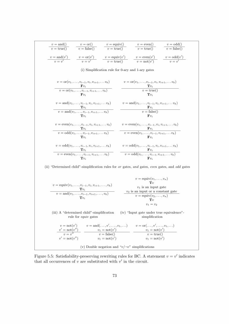
v = and()
v = true()
v = or()
v = false()
v = equiv()
v = true()
v = even()
v = true()
v = odd()
v = false()
v = and(v′)
v = v′v = or(v′)
v = v′v = equiv(v′)
v = true()
v = even(v′)
v = not(v′)
v = odd(v′)
v = v′
(i) Simplification rule for 0-ary and 1-ary gates
v = or(v1, . . . , vi−1, vi, vi+1, . . . vk)Fvi
v = or(v1, . . . , vi−1, vi+1, . . . vk)Fvi
v = or(v1, . . . , vi−1, vi, vi+1, . . . vk)Tvi
v = true()Tvi
v = and(v1, . . . , vi−1, vi, vi+1, . . . vk)Tvi
v = and(v1, . . . , vi−1, vi+1, . . . vk)Tvi
v = and(v1, . . . , vi−1, vi, vi+1, . . . vk)Fvi
v = false()Fvi
v = even(v1, . . . , vi−1, vi, vi+1, . . . vk)Tvi
v = odd(v1, . . . , vi−1, vi+1, . . . vk)Tvi
v = even(v1, . . . , vi−1, vi, vi+1, . . . vk)Fvi
v = even(v1, . . . , vi−1, vi+1, . . . vk)Fvi
v = odd(v1, . . . , vi−1, vi, vi+1, . . . vk)Tvi
v = even(v1, . . . , vi−1, vi+1, . . . vk)Tvi
v = odd(v1, . . . , vi−1, vi, vi+1, . . . vk)Fvi
v = odd(v1, . . . , vi−1, vi+1, . . . vk)Fvi
(ii) “Determined child”-simplification rules for or gates, and gates, even gates, and odd gates
v = equiv(v1, . . . , vi−1, vi, vi+1, . . . , vk)Tvi
v = and(v1, . . . , vi−1, vi+1, . . . , vk)Tvi
v = equiv(v1, . . . , vn)Tv
v1 is an input gatev2 is an input or a constant gate
v = equiv(v2, . . . , vn)Tv
v1 = v2
(iii) A “determined child”-simplification (iv) “Input gate under true equivalence”-rule for equiv gates simplification
v = not(v′)v′ = not(v′′)
v = v′′
v′ = not(v′′)
v = and(. . . , v′, . . . , v1, . . .)v1 = not(v′)
v = false()v1 = not(v′)
v = or(. . . , v′, . . . , v1, . . .)v1 = not(v′)
v = true()v1 = not(v′)
(v) Double negation and “v/¬v” simplifications
Figure 5.5: Satisfiability-preserving rewriting rules for BC. A statement v = v′ indicatesthat all occurrences of v are substituted with v′ in the circuit.
73

v := ite(vc, v1, v2)Tv
v := v1
v := ite(vc, v1, v2)Fv
v := v2
v := ite(vc, v1, v2)Tv1
Tv2
v := true()
v := ite(vc, v1, v2)Fv1
Fv2
v := false()
v := cardyx(v1, . . . , vi−1, vi, vi+1, vn)
Fvi
v := cardyx(v1, . . . , vi−1, vi, vi+1, vn)
v := cardyx(v1, . . . , vi−1, vi, vi+1, vn)
Tvi
v := cardy−1x−1(v1, . . . , vi−1, vi, vi+1, vn)
v := cardyx(v1, . . . , vk)
x ≤ 0 ∧ y ≥ k
v := true()
v := cardyx(v1, . . . , vk)
x > y ∨ y < 0 ∨ x > k
v := false()
Figure 5.6: Additional rewriting rules for “ite” gates and cardyx gates.
• A structural hashing scheme is employed in order to remove redundant gates.Remember that expand(f) refers to the exhaustive replacement of gate-functionarguments by their respective associated gate formulas. Given two gates g1 andg2 in a constrained circuit (C, τ), if expand(fg1) = expand(fg2), i.e., if they arefunctionally identical, we can remove g2 and replace all occurrences of g2 in theother gate equations with g1. In structural hashing, some functional equalities areefficiently found by merging structurally identical gates in a bottom-up fashion.
Such a substitution will yield an equisatisfiable constrained circuit instance as longas neither of the gates involved in merging is assigned a value in τ . Otherwise, itis necessary to propagate the gate assignments in τ in the constrained circuit overthe two gates. If, for a merged pair of gates (g1, g2), it holds that τ(g1) 6= τ(g2),then the original constrained circuit is unsatisfiable. If τ(g2) is defined, but notτ(g1), or vice versa, then we must propagate this assignment to the unassignedgate for the new instance to be equisatisfiable.
• Finally, a number of rewriting rules for creating an equisatisfiable instance areintroduced in [26]. These are shown in Figure 5.5. A statement g1 = g2 in arewriting rule, where both g1 and g2 are gates, indicates that all occurrences ofg1 are replaced by g2 in all gate equations. Similar to structural hashing, gateassignments must be propagated over gates that are substituted.
Similar to the case of the tableau rules, we present additional rewriting rules for itegates and card gates in Figure 5.6. Although such rules were not presented in theoriginal paper by Junttila and Niemela [26] where the BC tableau was introduced,we suspect that the same or similar rewriting rules are implemented in BCSat.
74

The same three strategies were implemented for our solver BattleAx3. We will give amore detailed description of the reduction process in Section 5.2 and describe a schemefor iterative circuit reduction during the solving process.
5.1.3 Tableau-Based SAT as Generalized DLL
For implementing the BC procedure, Junttila and Niemela [26] propose to apply thedeterministic deduction rules exhaustively before branching with the explicit cut rule.Since the BC-tableau rules extend a branch only with assignments nodes and not withgate equations, we can view a depth-first expansion of the tableau of an instance (C, τ) asa process of iteratively enlarging the partial assignment τ and subsequent backtrackingwhen a branch is closed.
In this way, the BC procedure can be implemented as a generalized DLL-procedure[14] for circuit instances. The application of the deterministic deduction rules is a gen-eralization of BCP, and the atomic cut rule corresponds to a decision. Algorithm 5.1is such a generalized DLL framework which can be used to structure a tableau-basedsolver. Our program, BattleAx3, is a prototypical implementation of this framework,and extends it by many techniques occurring in CNF-based SAT solving.
Algorithm 5.1: Tableau-based SAT procedure in a generalized DLL framework.input : (C, τ) - a constrained Boolean circuitoutput: Satisfiability of (C, τ)
if applyDeterministicRules(C, τ) = Conflict thenreturn false;
while true doif branchComplete(C, τ) then
return true;applyAtomicCut(C, τ);while applyDeterministicRules(C, τ) = Conflict do
bLevel← analyze(C, τ);if bLevel < 0 then
return false;else
backtrack(bLevel);
As Drechsler et al. [14] point out, the link between deduction in the BC tableau anddeduction in DLL-based SAT on a Tseitin-transformed circuit instance is very strong.Consider as an example a gate v = or(v1, . . . , vn) and its translation to CNF via Tseitin,i.e.,
(v ∨ ¬v1) ∧ . . . ∧ (v ∨ ¬vn) ∧ (¬v ∨ v1 ∨ . . . ∨ vn).
Each clause can be considered to encode a number of implications. The BC rules canthen be viewed as explicitly representing those implications. The first n binary clauses
75

of form (v ∨ ¬vi), for example, encode both the “Up”-rule stating that v must be true(vi ⇒ v), whenever any input is true, as well as the “Down”-rule that sets all inputs tofalse if the output v is false (¬v ⇒ vi). For more complex gate types such as card gates,“odd” gates or “even” gates, the CNF translation becomes increasingly cumbersome,since the rules are much more concisely expressible in arithmetic than by enumeratingall implications.
At this point, it is interesting to make the following observation regarding thestructure-preserving translation procedure presented in [37]. Remember that there, someclauses are possibly omitted from a gate’s translation depending on its polarity. Sincethe clauses correspond to certain rules in the BC tableau, we may build a new tableausystem that is still refutationally complete and sound by restricting the rules that areapplied to each gate to those that would be encoded in the polarity-based translation.
Consider as an example again the or gate shown above. If this gate has positivepolarity w. r. t. the formula to be checked, we can restrict the rules that are applied toit to the rules that are encoded in the clause
(¬v ∨ v1 ∨ . . . ∨ vn).
To be exact, it is sufficient in this case to restrict rule applications on this gate to theapplication of the “Last unassigned child” rule, and the F-“Up” rule. Such restrictionsmay be useful in implementation for two reasons. Such a restriction may allow for moreefficient implementation of the rules. There may be, on the other hand, drawbacksconcerning the increased length of minimal proofs, since we are essentially removingdeduction shortcuts from the circuit.
5.1.4 BC with Learning and Non-Chronological Backtracking
A straightforward implementation of the BC procedure would expand branches in adepth-first manner. Upon determining that a branch is closed, such an implementationwould continue to expand the most recent branch that is still incomplete. From theframework of Algorithm 5.1, it is easy to see that the BC tableau can be implementedin a way that is very similar to modern implementations of the DLL procedure. It isthen also possible to expand a BC-based solver with techniques that are popular inCNF-based SAT such as non-chronological backtracking and learning.
This requires a concept similar to that of the implication graph in CNF-based SAT,only for tableau rules. On a branch B = (b1, . . . , bi−1, bi, bi+1, . . . bk), we call a set oftableau nodes R = {r1, . . . , rj} ⊆ {b1, . . . , bi−1} a reason for bi iff we can extend a tableauconsisting only of the branch r1 → . . .→ rj to a tableau r1 → . . .→ rj → h1 → . . .→ hlby applying a tableau rule, where bi ∈ {h1, . . . , hl}. More informally, a set of tableaunodes R is a reason for another tableau node b iff we can deduce b using only the nodesin R. A reason R = {r1, . . . , rj} for a tableau node b is minimal iff, for any i with1 ≤ i ≤ j, it holds that R\{ri} is not a reason for b.
Remember that an assignment node is a tableau node of the form Tv or Fv. Areason assignment A for a node b is the subset of all assignment nodes in a reason R forb. The reason assignment A is minimal iff the underlying reason R is minimal.
76

Note, that there may be multiple minimal reason assignments for a single tableaunode. First, a node may be deduced on a branch using different tableau rules or differentgates. This is similar to the case of CNF-based SAT, where a single assignment mightbe derived using multiple clauses. Second, even with a single tableau rule application ona single gate, there may be multiple minimal reasons. When applying the F “Up”-rulefor an equiv gate g, for example, each pair of assignments (Tv1,Fv2) where v1 and v2
are children of g is a minimal reason assignment for Fg.Remember that a root tableau of a constrained circuit instance is its initial tableau
before any rule is applied. We can now define the concept of a generalized implicationgraph in the following way:
Definition 22. Let T be a BC tableau for a constrained circuit (C, τ). For a branchB = (b1, . . . , bk) in T , let Assign(B) denote the set of all assignment nodes in B. Wecall the the assignment nodes immediately after a cut-rule applications cut nodes. Then,a generalized implication graph of B is a graph (V,E) where
• V = Assign(B) ∪�, where the box node � is a special conflict node,
• for every node n in V that is not in the root tableau of (C, τ) and that is not a cutnode, the set of antecedents { n′ | (n′, n) ∈ E} is a minimal reason assignment forn,
• for every node n in B that is in the root tableau and for every cut node, the set ofantecedents is empty, and
• the antecedents of the conflict node � are the set of tableau nodes { n, n′ | n =Tv, n′ = Fv } ⊂ B.
We can manage a generalized implication graph in an implementation of a tableauprocedure by associating every deduced assignment node n with the assignment nodesthat caused n to be deduced. Since there may be multiple minimal reason assignmentsfor a tableau node, multiple implication graphs are possible.
We can use this generalized implication graph analogously to the CNF case in orderto perform learning and non-chronological backtracking. Notions such as responsibleassignments, separating cuts, and the different strategies for choosing a cut can beextended to this generalized implication graph in a straightforward way. The decisionlevel of a branch is the number of cut rule applications on that branch. A learnedclause can be viewed as a fresh or gate with its output constrained to true. For theinput literals, new not gates may have to be added. The resulting structure can then besimply added to the circuit to gain an equisatisfiable instance.
In order to leave the basic BC tableau unchanged, we choose to view learning and non-chronological backtracking as a procedure that transforms a BC tableau for a constrainedcircuit to a BC tableau for another constrained circuit. The latter constrained circuit isthe result of extending the former constrained circuit with the added learned gate and theconflict-driven assertion. This is illustrated in Figure 5.7. We refer to this transformationas folding the original tableau with respect to a responsible conflict assignment. The
77

v1 := or(v2, v4)
v4 := even(v2, v3, v5)
v5 := or(v2, v3)
Fv1
(19) Fv2
(19) Fv4
(1) Tv5
(23) Tv3
(13) Tv4
(1) Fv5
responsibleassignment
v6 := or(v7, v1)
v7 := not(v5)
v1 := or(v2, v4)
v4 := even(v2, v3, v5)
v5 := or(v2, v3)
Fv1
Tv6
(19) Fv2
(19) Fv4
(23) Fv5
learned nodes
conflict-drivenassignment
fold
unfold
Figure 5.7: An illustration of learning and non-chronological backtracking in the BCtableau.
reverse process, where all unit-rule applications on learned gates are substituted bysubtableaus, we refer to as unfolding.
After arriving at a finished folded BC tableau with the generalized DLL procedure, wecan exhaustively unfold it in order to obtain a finished tableau of the original constrainedcircuit instance.
5.1.5 Datastructures for Deduction
Since, similar to CNF-based solvers, the application of deduction rules takes up mostof the runtime in a BC-based tableau solver, efficient implementations are of high im-portance. We have already presented some of these options in Chapter 4. Here, wewill give a more compact overview of different implementation techniques for deductionin circuit structures before we explain our implementation choices for BattleAx3 in thenext section. The overview will be based in part on the work in Drechsler et al. [14].
78

Counter-Based Deduction
A simple possibility for determining the applicability of tableau-rules is to keep countersfor each gate that describe the number of positive and negative inputs. Each gate keepsreferences to its parent gates, and when a formerly unassigned gate is assigned a value,the appropriate counter of the parent is incremented by one. In BCSat, such a counter-based approach was used [25].
Rule applicability conditions can then be easily formulated as algebraic checks onthe counters, e.g., if, for an and gate g, it holds that the number of children equals thenumber of true inputs, the and “Up”-rule is applicable, and we can deduce Tg.
One disadvantage of this approach is that in backtracking, all the counters need to bereset. Compared with stateless or lazy datastructures, this is a significant disadvantage.
Implication Lists
For all those tableau rules in which a single assignment Tv or Fv is a sufficient conditionfor a rule’s applicability, performing algebraic checks on counters is a significant overheadcompared with a naive, straightforward implementation. This is similar to the case ofbinary clauses in CNF, where highly-tuned solvers use direct implication lists. Thisapproach finds applications, for example, in the circuit-solvers presented in Thiffaultet al. [46] and Wu et al. [51].
In the BC tableau, we can use implication lists for both the “Up” rule and the“Down” rule for not gates, for the F-“Up” rule and the T-“Down” rule for and gates,and for the F-“Down” rule and the T-“Up” rule for or gates.
The use of implication lists changes the structure of the search, since all direct im-plications are assigned in one step, either before or after tableau rule application. Thereis disagreement in the literature as to whether this yields performance increases or de-creases in the case of CNF-based solvers. In Biere [3], the author argues that the cheaperdirect-implications should be used exhaustively before using the more expensive unit-rule. In MiniSAT [39], on the other hand, the direct implication list is directly integratedinto the literal watch lists in order to avoid this separation of direct implications andunit-rule applications. The authors argue that the separation of rule applications yieldsslightly less useful conflict clauses.
Lookup Tables
If a circuit representation is chosen which is restricted to a certain arity for gates, lookuptables can be used in the deduction step. Such an approach is presented in Kuehlmannet al. [29] for an and-inverter-graph (AIG) circuit representation. In an AIG, each gateis either an and gate with a fixed arity of two, or a not gate.
For a constant-arity gate, each possible combination of true, false and unassignedinput and output values can be represented as an entry in a table. These table entriesencode the assignments that can be deduced given the current partial assignment. Inaddition, the table encodes whether a partial input assignment is conflicting. Given apartial assignment to a gate, the table can then be queried in constant time.
79

Since no state information is saved for gates in this scheme, no action needs to beperformed in backtracking to keep rule status consistent.
Generalized Watching Schemes
Some attempts have been made to extend the watching schemes used in CNF-based SATsolvers to gate structures. In Thiffault et al. [46], a watching scheme is proposed for andgates and or gates.
For or gates, such a scheme is virtually identical to the watched-literal scheme inCNF-based SAT. The main difference between clauses and or gates concerning deductionis that a clause’s output is implicitly constrained to true, while an or gate’s output mayalso become false without necessarily causing a conflict.
It is then easy to see how the watched-literal scheme can be translated to circuitstructures. For each or gate g, two inputs are watched. The invariant over these twowatched inputs is that neither of them may become false. If this invariant cannot bemade true by moving the watched input after an assignment, then one of two cases holds:If the other watched input is already false, conclude Tg. Otherwise, if the other watchedinput is unassigned, check whether Tg holds. If it does, assign the other watched inputto be true. This procedure basically encodes the F-“Up” rule and the “Last unassignedchild” rule for or gates. The other rules are implemented in a straightforward manner.
For and gates, the idea is analogous, only with the roles of T and F values reversed.Two input gates are watched, the invariant being that neither of them may become true.If this invariant cannot be made true by moving watched inputs, the T-“Up” rule or the“Last unassigned child rule” may be applicable.
Recently, the solver QuteSAT was presented in Wu et al. [51] in which the watch-ing scheme is extended to arbitrary gate types. The authors distinguish two types ofinference over gates, called direct implications and indirect implications. Direct impli-cations are those inference rules that are applicable due to a single assignment. Thesecorrespond to binary clauses in the CNF translation of the circuit. Deduction for directimplications is handled via a form of implications lists. Indirect implications are thoseinference rules whose applicability depends on more than one assignment. For indirectimplication, the generalized watching scheme is used.
For the simple gate types and and or, the watching scheme is similar to the watched-literal scheme on the Tseitin transformed CNF. So, for a gate v := or(v1, . . . , vn), twoof the pairs in {(v,F), (v1,T), . . . , (vn,T)} would be watched, the invariant being thatthe variable in a watched pair (v,X) may not be assigned the opposite value to X (thischaracterization of the scheme is taken from Drechsler et al. [14]). This is similar tosimply watching the clause ¬v ∨ v1 ∨ . . . ∨ vn in the watched-literal scheme. For andgates, deduction is handled analogously, but with the roles of T and F reversed.
For more complex gate types, another watching scheme is used. In a gate v =f(v1, . . . , vn), we call a variable in {v, v1, . . . , vn} a watch candidate iff its assignmentcan lead to an indirect implication. In such a gate, we watch a number of l watchcandidates, the invariant being that the watched variables are unassigned.
80

If the invariant cannot be made true by moving the watch pointer to an as-of-yetunwatched watch candidate, the gate function is used to determine values for the unas-signed gates. The number of necessary watched inputs l can be determined by findingthe smallest number of assignments k on a gate’s inputs and output that trigger an indi-rect implication. For a gate with m watch candidates, the number of necessary watchedinputs is then l = m− k + 1.
As an example, consider a gate v := odd(v1, . . . , vn). The set of watch candidatesis {v, v1, . . . , vn}, therefore m = n + 1. Since we can only make an implied assignmentonce all but one watch candidates are assigned, it holds that k = n and l = m− k+ 1 =(n+ 1)− n+ 1 = 2. We therefore need to watch two candidates. Once it is impossibleto uphold the invariant, i.e., when all but one watch candidates are assigned, we use theodd gate-function in order to determine the remaining assignment.
Note that, for some gates, the value of l may be rather high. For an equiv gate ofarity n, for example, l = n. In such cases, the use of watch pointers may become moreinefficient than using counters.
5.2 Implementing an Enhanced Tableau-Based Solver
While the basic DLL algorithm is conceptually rather simple, modern SAT solvers arehighly complex pieces of software whose components interact non-trivially. Implement-ing a SAT solver calls for many small implementation choices which are rarely describedin detail in the literature. Seemingly small changes in the implementation can cause bigeffects. Biere [3] describes, for example, how an undocumented detail of the implemen-tation of the learning strategy in Chaff [34] improved performance considerably.
Some of these omissions may be rooted in an underestimation of the importance ofa given implementation choice. More often though, these omissions can be attributed toa lack of space. An exhaustive description of a solver implementation is simply beyondthe scope of most papers.
In this section, we will describe a prototypical implementation of the frameworkpresented in Section 5.1. We have developed BattleAx3, a BC-based SAT solver withnon-chronological backtracking and learning. Furthermore, the basic BattleAx3 imple-mentation was extended with a number of techniques from CNF-based SAT in order toevaluate their efficiency in circuit instances.
Since we do not suffer from the space constraints of a paper, we have chosen to givea fairly detailed description of BattleAx3, although not an exhaustive one. We givesome information about implementation basics, which are otherwise rather sparse in theliterature. Besides studying existing implementations of CNF-based SAT solvers whosesource code is openly available (e.g., MiniSAT [39]), the descriptions in Biere [4] provedvery helpful for solving many technical details.
81

−3 6 −4 7 −5 10
0 1 2
2 3 5
decision level
trail
control
Figure 5.8: Trail stack and control stack.
5.2.1 Basic Datastructures
In BattleAx3, the circuit is represented as an array of gates. Each gate structure containsa field indicating the type of the gate, a reference to an array containing the array indicesof children, and a reference to a second array indicating the array indices of parents.
The current partial assignment is also stored in an array, which indicates for eachgate index whether the gate is unassigned, true, or false. In order to keep track of theorder of assignments and of the assignments made on each decision level, we use twostacks.
One stack, referred to as the trail stack, contains all assignments that were made onthe current branch of the tableau in the order in which they were made. Essentially, itis a direct representation of the assignment nodes on the current tableau branch. Anassignment node is represented as an integer indicating the index of the assigned array.A positive integer denotes an assignment node of the form Tv, a negative integer denotesan assignment node of form Fv. Whenever a variable is assigned a value, either due toa decision or a deduction, it is put on top of this stack.
The second stack, called the control stack, contains values indicating the size of thetrail stack at the end of each decision level. Initially, the control stack is empty. Eachtime before a decision is made, i.e., before the decision level is increased, the current sizeof the trail stack is put on the control stack. In backtracking, the information on thecontrol stack is used to identify the decisions that have to be undone. An illustration ofboth stacks is given in Figure 5.8.
5.2.2 Deduction
The main datastructure involved in the deduction process is the assignment queue.Whenever a variable is assigned, it is appended to the assignment queue. In the de-duction step, each assignment in turn is taken off the queue and the necessary deductionrules are applied. These may generate new assignments, which are again appended tothe queue. The whole process is repeated until either a conflicting assignment is pro-duced or until the assignment queue is empty. The procedure is sketched in Algorithm
82

5.2.
Algorithm 5.2: The applyDeterministicRules step in Algorithm 5.1.while ¬isEmpty(assignmentQueue) do
assignment ← removeFirst(assignmentQueue);deducedAssignments← fireApplicableRules(assignment);τ ← τ ∪ deducedAssignments;appendAll(assignmentQueue, deducedAssignments);
The fireApplicableRules step in Algorithm 5.2, can be implemented for an assign-ment v as follows.
(i) Check for all parents of var(v) whether any “Up” rules or “Last unassigned child”rules are applicable.
(ii) Check for gate v itself whether any “Down” rules or “Last unassigned child” rulesare applicable
Instead of a queue, a stack could also be used to store assignments. This wouldlead to a depth-first exploration of deduced assignments, in contrast to the breadth-firstexploration effected by the queue implementation we use. Biere [3] remarks that theuse of a queue heuristically minimizes the implication graph, which keeps the length oflearned clauses low.
Biere [3] also explores the use of lazy assignments. This means that whenever avariable assignment is deduced or decided, it is only put on the assignment queue. Theactual variable assignment is delayed until the variable is dequeued during the deducestep. This contrasts with the more common technique of busy assignments, i.e., settingits value and putting it on the trail stack as soon as its value is deduced or decided.The advantage in lazy assignments is that, since a variable assignment is not madeimmediately after it is deduced, it may be deduced a second time by another clause. Inthis way, multiple reasons can be recorded for each variable assignment.
Biere [3] suggests that such a strategy is not ideal. While lazy assignments allowfor the identification of multiple reasons for a single conflict which can be heuristicallyused to produce small conflict clauses, it leads to complications in the overall design of asolver which are not worth the possible speedups. In our implementation, we thereforeuse busy assignments, which is the implementation choice in most solvers.
We have chosen to implement deduction using three distinct implementation strate-gies. For normal gates, counters are used. While this may not be the most efficientchoice on average, it is easy to implement and allows for equally efficient encoding ofall gate rules in the BC tableau. The BC tableau includes not only simple gate types,but complex ones such as equiv and card gates. A generalized watched-input schemeas in Wu et al. [51] would likely be inefficient on instances that rely heavily on thosegate types since the rules would need to be checked nearly as often as in a counter-basedapproach, but each check requires effort linear in the size of the gate. It is still likely
83

that the average runtime of the solver could be decreased for many classes of instancesif a watched pointer scheme was implemented for some gate types.
As a second type of deduction, we have implemented the option to use implicationlists for simple rules whose firing condition depends on a single variable assignment.If this option is activated, all implication-list deductions are made before the ordinarytableau rules are fired. This changes the structure of the search since deductions aremade in a different order which leads to a different implication graph. Furthermore,there is an option to apply implication-list deduction exhaustively before going on to theapplication of the remaining rules, as it is suggested in Biere [3].
The third kind of deduction is used for learned clauses. While it would be possibleto represent learned clauses as or gates with outputs that are constrained to true, adirect representation seems more natural and is likely to be more efficient. We use thewatched-literal scheme for deduction [34]. The watched literals are kept at the first andsecond position of a clause as it is outlined in Biere [5], which avoids the use of a separatewatcher datastructure.
5.2.3 Conflict Analysis, Learning and Backjumping
We have already introduced the notion of a generalized implication graph for the BCtableau procedure. Our solver successively builds up such a graph for the current branchby storing a minimal reason assignment for each derived tableau node. In CNF-basedSAT, the implication graph is usually represented implicitly by storing only a pointer toa clause for each assignment. The full graph can be retrieved by analyzing the literals inthese clauses. Since the tableau format is more heterogeneous than CNF, we explicitlyassociate a stack of integers with each gate which record its reason assignments.
In some cases, multiple reason assignments may be found for a single tableau ruleapplication. While it would be interesting to evaluate different strategies for choosingamong those reasons, we use no such heuristic, but simply use the first applicable reasonassignment that is identified in the analysis step.
In Kuehlmann et al. [29], an alternative way of implementing an implication graphis presented. There, each circuit gate g is associated with a bit vector representing thedecisions that are ultimately responsible for the current value of g. If two gate values areused to deduce a third, the third value is associated with the result of applying a bit-wiseor operation to the bit vectors of the first two gates. When a conflict is derived, a bit-wiseor operation on the conflicting gate assignments’ bit vectors instantly yields a responsibleassignment. This strategy can be seen as a busy variant of the analysis procedure inmodern CNF-based SAT solvers. When a conflict is derived, we immediately gain aresponsible assignment, but more work needs to be done during deduction. Such anapproach is not ideal for our purposes since it would entail a large amount of overheadduring deduction in large circuits. Furthermore, it is not clear how one can implementefficient learning approaches such as the first-cut scheme using this technique.
We use the first-cut scheme for clause learning that was already presented in Chapter3. In the first-cut scheme, the conflict clause contains the UIP closest to the conflict
84

node (the first UIP) together with all assignment nodes from earlier decision levels thathave an edge to an assignment on the conflict side of the partition induced by the UIP.
The identification of the first UIP can be performed in a single traversal of theimplication graph by going backwards from the conflict node and counting “open paths”.Algorithm 5.3 (taken from [4]) sketches an efficient procedure for identifying the conflictclause induced by the first cut. The number of open paths is initialized to the antecedentsof the conflict node in the generalized implication graph. Then the implication graph istraversed backwards from the conflict node in the order indicated by the trail stack (i.e.,the most recent assignment node is visited first), ignoring all assignments nodes that donot have a path to the conflict node. When a node is visited, the number of open pathsis decremented by one, and incremented by the number of unvisited children that are onthe most-recent decision level. When the number of open paths reaches one, the nextassignment node that is visited is the UIP.
Algorithm 5.3: Identifying the first cut.conflictClause← ∅;openPaths← 0;for each assignment ∈ conflictReason do
if getDLevel(assignment) = conflictDLevel thenmark(assignment);openPaths← openPaths + 1;
elseconflictClause← conflictClause ∪ { litMadeFalseBy(assignment)};
while true doassignment← pop(trailStack);if isMarked(assignment) then
if openPaths = 1 thenreturn conflictClause ∪ { litMadeFalseBy(assignment)};
for each r ∈ reason(assignment) doif getDLevel(r) = conflictDLevel then
mark(r);openPaths← openPaths + 1;
elseconflictClause← conflictClause ∪ { litMadeFalseBy(r)};
openPaths← openPaths− 1;
Learned clauses are stored in a monolithic memory array. This necessitates additionalgarbage collection code, but is slightly more cache efficient than using normal memoryallocation. Clauses are deleted based on their recent activity in a VSIDS-like scheme.Each clause is associated with a counter. This counter is increased twice each time aclause is conflicting, and once for each clause that was used to derive the conflict on themost recent decision level.
85

5.2.4 Circuit Reduction
As was explained earlier, three techniques for reducing the size of a circuit are imple-mented,
• a cone-of-influence reduction,
• a structural hashing scheme, and
• the rewriting rules in Figure 5.5 and Figure 5.6.
These rules are applied at preprocessing and whenever a one-literal clause is learned.A one-literal clause triggers a backtrack to decision level 0 and effectively restarts thesolver with an added constraint on the circuit instance. This added constraint allows areapplication of the rewriting rules, which in turn opens up new possibilities for reductionwith the other two approaches. In some instances, one-literal clauses are learned veryfrequently. There, the resulting frequent circuit reductions can take up a significantamount of the runtime. In order not to impede overall efficiency in such cases, we donot apply circuit reduction after every learned one-literal clause, but count the numberof learned one-literal clauses since the last reduction step. When this number reaches afixed threshold, circuit reduction is applied.
After reducing the circuit, the following rules are applied to each clause c in theclause database:
• If a literal in c corresponds to a gate that was removed in the cone-of-influencereduction, remove c from the clause database.
• If a literal l in c corresponds to gate that was substituted by another gate usingthe rewriting rules or the structural hashing scheme, replace l by the same-phaseliteral on the substitute gate.
• If a literal l in c is false at decision level 0, remove l from c.
• If a literal l in c is true at decision level 0, remove c from the clause database.
5.2.5 One-Step Lookahead
We have implemented the option of using a one-step lookahead rule, which was proposedin Junttila and Niemela [26]. This rule states that, if we can deduce a conflict using thedeterministic deduction rules after “trying out” a lookahead assignment Tv (Fv) on abranch, we can immediately deduce Fv (resp. Tv).
In a solver with non-chronological backtracking and learning, we can implementlookahead as a straightforward decision. The difference is that if no conflict occurs asan immediate result of the decision, we backtrack chronologically and possibly try out anumber of other lookahead assignments in the same way. If, on the other hand, a conflictoccurs as a result of the lookahead assignment, we can learn a conflict clause using thefirst-cut scheme and backtrack non-chronologically. Considering the lookahead rule from
86

the perspective of the generalized DLL procedure, this is essentially an introduction oflocal breadth-first search at each node in the depth-first search tree. This idea is sketchedin Figure 5.9.
...
S
S1 · · · Sk �︸ ︷︷ ︸Non-conflicting
lookahead assignments
Conflict in lookahead:learn clause, backtrack
Figure 5.9: A partial search tree of the generalized DLL procedure using the lookaheadrule.
In Junttila and Niemela [26], the authors seem to propose an unrestricted applicationof the lookahead heuristic where, in each step of the search, all unassigned variables areused as lookahead assignments. Such an implementation was evaluated in BattleAx3, butwas found to be highly inefficient on some benchmarks. We have implemented a numberof different restrictions in order to try increasing the robustness of the strategy. Onepossible restriction is to apply lookahead only to children of unjustified gates. Anotherone is to combine the lookahead scheme with the VSIDS heuristic for variable selection.
In our implementation, VSIDS literals are stored in a heap so that the literal withthe highest score can be retrieved efficiently during the decision step. The heap itself isimplemented as an array. We can restrict our lookahead to the first n variables found inthe heap’s literal array. While these may not be the n highest-scoring VSIDS literals, itstill yields an efficiently computable heuristic for applying lookahead only for variablesthat are somewhat likely to lead to conflicts.
The implementation of the lookahead rule can be sped up significantly by markingassignments that are derived during a lookahead. Such assignments cannot lead toconflicts and therefore do not need to be tried out as lookahead assignments on the samedecision level. As an example, consider a lookahead assignment Tvl from which Fv canbe derived inside the lookahead. Assume that the lookahead assignment does not leadto a conflict. Now it is clear that in subsequent lookaheads on the same decision level,we can skip the lookahead assignment Fv, since this assignment was already made as aconsequence of Tvl.
5.2.6 Decision Variable Selection
We have implemented three different strategies for choosing decision variables: the pop-ular VSIDS and BerkMin heuristics, both of which were described in Chapter 3, and
87

the lookahead decision heuristic that builds upon the lookahead rule described in theprevious section and was the decision heuristic used in BattleAx3.
The VSIDS scheme is implemented using a priority queue with an underlying heap.During decision variable selection, elements are repeatedly removed from the front ofthe queue until a literal is found whose variable is unassigned. In BerkMin, the decisionheuristic chooses a literal from the the top clause, which is the most-recently learnedclause that is not satisfied. A naive implementation can lead to a majority of the runtimebeing spent in the decision heuristic in search of the top clause. This can be solved bycaching its position between conflicts.
In the lookahead heuristic, we count the number of rule applications that can beperformed as a consequence of the lookahead assignments. Let vF and vT be the numberof new assignment nodes that can be deduces from an assignment Fv respectively Tv.The lookahead heuristic then chooses a decision variable v for which min(vF, vT) ismaximal.
In addition to the heuristics outlined above, each heuristic can be combined withjustification filtering and phase saving. In justification filtering, only those variablesare considered for decisions which have unjustified parents. Justification filtering entailssignificant overhead since a justification frontier has to be maintained.
Phase saving was already described in Chapter 3. Here, the phase of a decisionvariable v is set to be the last phase that variable was assigned to. In this way, some ofthe progress that was lost due to non-chronological backtracks and restarts can quicklybe regained.
5.2.7 Restarts
For our solver BattleAx3, we also adopt the use of random restarts. Here, the solver isreset at certain points during the search to decision level 0, but with the database oflearned clause intact. We introduce some transient randomness to allow the solver toenter new regions of the search space.
Restarts are usually triggered after a certain number of conflicts or decisions. Thisnumber should be successively increased in order for the solver to stay complete. Choos-ing such a sequence of restart limits is a main consideration in implementing restarts.
We have implemented three different strategies for this purpose:
• A simple strategy where the restarting and clause limit are increased geometrically,starting with an initial value of 100 for the restarting limit, and the number of gatesdivided by two for the clause limit. At each restart, the restarting limit is increasedby 50% and the clause limit by 10% (parameters taken from [39]).
• The nested restarting strategy used in PicoSAT [5], where two limits are used, theactual restart limit and an outer limit (both with an initial value of 100). Therestart limit is increased by 10% at each restart. Upon reaching the outer limit,the restart limit is reset to an initial value, and the outer limit is increased by 10%.The clause limit is increased by 5% each time the outer limit is increased.
88

• The RSAT2.0 strategy [36] (originally motivated by the work in Huang [22]), wherethe Luby sequence [31] is used as a basis for the restart limit sequence. The Lubysequence is the sequence t1, t2, t3, . . . such that
ti ={
2k−1, if i = 2k − 1ti−2k−1+1, if 2k−1 ≤ i < 2k − 1
and has the prefix
1, 1, 2, 1, 1, 2, 4, 1, 1, 2, 1, 1, 2, 4, 8, 1, 1, 2, 1, 1, 2, 4, 1, 1, 2, 1, 1, . . .
We follow the suggestion in Pipatsrisawat and Darwiche [36] and set the unit forthe Luby sequence to 512 conflicts, i.e., the actual sequence of restart limits is512, 512, 1024, 512, . . .. Furthermore, we increase the clause limit by 15% every 2k
restarts.
At each restart, we perform circuit reduction if any one-literal clauses were learnedduring the last restart interval.
89

Chapter 6
Results
In this chapter, we will evaluate some of the techniques implemented in BattleAx3 using abenchmark set of 38 instances introduced in Jarvisalo and Niemela [23]. The benchmarksare given in the BC1.0 format [24] which allows to express circuit structures by definingtheir gate equations. The problems are taken from the domains of
• verification of superscalar processors,
• integer factorization based on hardware multiplier designs,
• equivalence checking of hardware multipliers,
• bounded model checking for deadlocks in LTSs, and
• linear temporal logic BMC of finite state systems.
Some simple statistics over the instances in the benchmark set, including the num-ber of gates, the average number of children in non-input gates, and the average andmaximum path lengths between primary inputs and outputs, are shown in Table 6.1.The numbers are derived from BattleAx3’s parsing engine. Note that, due to some im-plementation choices, the number of gates shown here may be slightly higher than theactual number of gates defined in the instances.
All benchmarks presented in this chapter were performed on a Linux workstationwith 2 GB of RAM and an Intel Core 2 Quad Q6600 processor overclocked to 3.0 GHz.In each case, two benchmark instances were run concurrently, as this did not seem toaffect overall runtime. The timeout was set at 1800 seconds.
6.1 Comparing Decision Heuristics
In Table 6.2, a comparison between the VSIDS and BerkMin heuristic is given. InVSIDS, the literal with maximum associated score is chosen for assignment, while inBerkMin, the maximum-score literal of the top clause, i.e., the most recently learnedclause that is not satisfied, is chosen. According to Goldberg and Novikov [19], the
90

# instance name no. avg. no. avg. path max. pathgates children (in→out) (in→out)
1 1394-4-3.p1neg.k10.unsat 67904 2.02 9.86 2122 1394-4-3.p1neg.k11.sat 74357 2.02 9.86 2133 1394-5-2.p0neg.k13.unsat 88882 1.87 9.46 1944 atree.sat.34.0 12965 2.48 4.90 635 atree.sat.36.50 14333 2.49 4.98 666 atree.sat.38.100 15469 2.49 5.11 667 atree.unsat.32.0 11461 2.48 5.07 508 atree.unsat.34.50 12965 2.48 4.90 639 atree.unsat.36.100 14333 2.49 4.98 6610 braun.sat.32.0 6176 1.99 7.89 12711 braun.sat.34.50 6970 1.99 7.90 13512 braun.sat.36.100 7812 1.99 7.94 14313 braun.unsat.32.0 6176 1.99 7.89 12714 braun.unsat.34.50 6970 1.99 7.90 13515 braun.unsat.36.100 7812 1.99 7.94 14316 brp.ptimonegnv.k23.unsat 18087 1.82 8.11 21417 brp.ptimonegnv.k24.sat 18869 1.82 8.11 22318 csmacd.p0.k16.unsat 105550 2.23 8.43 14719 dme3.ptimo.k61.unsat 57973 1.92 7.60 105220 dme3.ptimo.k62.sat 58921 1.92 7.60 106921 dme3.ptimonegnv.k58.unsat 55020 1.93 7.80 100222 dme3.ptimonegnv.k59.sat 55966 1.93 7.80 101923 dme5.ptimo.k65.unsat 100221 1.94 7.62 112024 dp 12.i.k10.unsat 5907 1.82 3.23 6125 eq-test.atree.braun.10.unsat 1978 2.27 3.51 4126 eq-test.atree.braun.8.unsat 1320 2.26 3.45 3327 eq-test.atree.braun.9.unsat 1745 2.28 3.58 3728 fvp-unsat.2.0.3pipe.1 2879 10.15 6.98 4229 fvp-unsat.2.0.3pipe 2 ooo.1 8299 5.68 6.83 5130 fvp-unsat.2.0.4pipe 1 ooo.1 19640 6.14 6.29 7731 fvp-unsat.2.0.4pipe 2 ooo.1 19966 6.44 6.91 7732 fvp-unsat.2.0.5pipe 1 ooo.1 37648 7.45 6.33 12333 key 4.p.k28.unsat 21765 1.89 3.41 19834 key 4.p.k37.sat 32727 1.96 3.70 26135 key 5.p.k29.unsat 27354 1.90 3.37 20536 key 5.p.k37.sat 39210 1.96 3.63 26137 mmgt 4.i.k15.unsat 10575 2.10 3.22 10738 q 1.i.k18.unsat 11064 1.76 2.66 123
Table 6.1: The BC benchmark set from Jarvisalo and Niemela [23].
91

BerkMin strategy makes the decision heuristic more robust by increasing the speed withwhich the solver adjust to new regions of the search space.
Overall, both heuristics seem to work nearly equally well in BattleAx3. The BerkMinheuristic proves fast for small instances, and manages to solve one more instance thanVSIDS in the 30-minute time limit. Still, VSIDS seems to be the better overall choicewith a lower combined runtime and a smaller number of average decisions.
An interesting observation can be made when studying the average clause lengthsand average decision levels of both strategies. Here, values differ drastically and in arather counter-intuitive way. VSIDS produces very long conflict clauses, but does not,on average, spend much of the search deep down in the search tree. BerkMin’s averagedecision level is three times deeper than that of VSIDS and the conflict clauses are onlyhalf as long on average, but it is slower overall.
First of all, this is an indication that the length of short conflict clauses is not a verygood indicator of the efficiency of a decision heuristic. Second, it may be an indicationthat increasing the locality of the search, as is done in BerkMin, may delay conflicts thatwould otherwise occur earlier, and therefore increase the average decision level.
The vast differences in average clause length and average decision level are ratherunexpected considering that both the BerkMin decision heuristic and VSIDS are basedon similar ideas. It might be worthwhile to analyze the interplay between decisionheuristics, average decision level, and average conflict complexity more closely. A betterunderstanding of these effects may yield, for example, more efficient decision heuristics ormeta-heuristics which dynamically alter decision heuristic parameters during the search.
6.2 Evaluating Lookahead
We have implemented the lookahead rule and the lookahead decision heuristic fromJunttila and Niemela [26], both of which are described in detail in Chapter 5. We havetried to answer the question of whether the application of this rule, which seems to haveworked well in BCSat [26], still manages to improve solving efficiency on the extendedtableau procedure.
In Table 6.3, a basic comparison between a straightforward application of the looka-head rule and lookahead decision heuristic, a restricted application of the same twotechniques, and the normal VSIDS-based approach are presented. It is obvious that theunrestricted application of the lookahead rule decreases solving efficiency considerably.At the same time, the number of actual decisions on the solved instances is decreased bytwo orders of magnitude using this strategy. Restricting the lookahead to the childrenof unjustified gates seems to increase efficiency somewhat compared to an unrestrictedlookahead, but there is still a significant performance drop compared to the VSIDSbaseline.
In Table 6.4, we have tried to explore restrictions of the basic lookahead rule further.Again, the left column shows the baseline results for the VSIDS decision heuristic withoutlookahead. We compare this with a restriction of the lookahead rule to the first 4 and 32literals in the VSIDS heap array (4VSIDSLH and 32VSIDSLH). We also evaluate using
92

VSIDS BerkMin# sat time dec- clause avg. time dec- clause avg.
(s) isions length dLevel (s) isions length dLevel1 no 139.99 280253 75.76 74.06 289.63 730389 65.96 86.102 yes 104.00 397522 47.55 115.40 292.34 917344 28.66 86.943 no 483.01 522928 157.54 86.07 448.20 759067 66.08 74.204 yes 132.80 189790 284.93 19.59 259.91 398720 255.78 15.865 yes 250.61 318747 239.52 28.12 339.70 561101 193.93 19.636 yes 83.23 137902 139.57 25.67 595.02 711945 285.35 20.387 no 381.01 484422 577.70 20.49 343.83 430269 234.84 13.138 no 403.24 425575 552.88 16.69 911.96 962775 596.54 13.899 no > 1800 1583.92 1402523 441.29 14.3610 yes 46.08 132492 156.57 17.63 132.54 345499 149.20 11.7311 yes 460.68 721780 354.73 22.61 354.18 711594 185.29 13.4912 yes 336.37 722126 376.44 25.37 8.93 55827 119.14 18.0113 no 165.92 323037 381.88 20.57 110.45 309481 125.01 11.7814 no 246.14 632974 298.01 20.02 290.53 708569 169.11 11.5415 no 809.52 1215931 323.65 27.50 788.31 1629242 219.75 12.5316 no 121.60 224553 111.83 25.65 124.11 262040 75.40 18.0917 yes 57.86 130666 77.60 34.39 102.66 226141 81.61 20.0618 no 1024.70 639245 163.00 52.18 > 180019 no 211.44 506279 322.71 78.02 262.61 705258 219.81 498.5020 yes 410.38 707957 389.89 157.39 30.01 660122 63.97 1634.6321 no 69.14 242506 207.22 79.72 59.16 512893 111.23 677.0122 yes 44.11 222240 178.68 411.80 12.99 295024 33.34 1108.3623 no 47.40 238891 146.98 103.62 1657.66 1454497 266.10 604.0124 no > 1800 > 180025 no 820.30 4827722 103.20 13.65 1251.49 6559621 82.39 12.4226 no 14.30 164324 67.04 11.66 21.08 256897 57.64 9.9827 no 122.89 993259 80.38 12.16 118.34 1063909 62.08 11.0728 no 1.72 59901 83.08 47.45 1.71 55296 93.12 35.1929 no 2.56 48552 106.52 34.68 1.26 23051 82.22 18.5430 no 11.02 129459 186.85 43.78 7.76 67413 181.59 21.3331 no 21.12 187714 237.68 47.77 10.81 80290 187.46 21.2932 no 41.78 296308 310.34 77.55 30.66 140095 323.45 24.8533 no 139.09 198997 692.28 62.02 138.22 287455 315.04 17.0334 yes 37.69 95608 399.16 66.64 22.55 140564 123.67 32.8935 no 363.86 354655 993.65 68.84 194.68 287101 420.37 21.2636 yes 464.60 531818 854.91 96.58 2.90 37924 29.39 39.9337 no 1051.50 1703756 410.92 45.21 638.07 1155698 242.71 15.7038 no > 1800 460.53 895742 274.21 14.52
lower avg. lower avg.bound over solved bound over solved
> 14521.66 543139.69 288.31 59.73 > 15498.71 737182.17 184.65 150.87inst.solved by both: inst.solved by both:
sum avg. sum avg.8096.96 540313.05 291.99 59.96 9854.26 691267 169.04 154.46
# solved 35 36
Table 6.2: Comparing VSIDS and BerkMin decision heuristics.
93

# sat VSIDS LH dec. heur. LH dec. heur.(no lookahead) (unrestricted) (just. restr.)
1 no 139.99 280253 > 1800 > 18002 yes 104.00 397522 > 1800 > 18003 no 483.01 522928 > 1800 > 18004 yes 132.80 189790 > 1800 > 18005 yes 250.61 318747 > 1800 1135.73 326776 yes 83.23 137902 > 1800 > 18007 no 381.01 484422 > 1800 1637.16 275718 no 403.24 425575 > 1800 > 18009 no > 1800 > 1800 > 180010 yes 46.08 132492 809.23 6977 796.52 3868711 yes 460.68 721780 1343.05 9156 675.37 4026712 yes 336.37 722126 > 1800 563.59 3006513 no 165.92 323037 736.22 4907 645.30 5747314 no 246.14 632974 > 1800 1677.35 6262415 no 809.52 1215931 > 1800 > 180016 no 121.60 224553 > 1800 > 180017 yes 57.86 130666 > 1800 > 180018 no 1024.70 639245 > 1800 > 180019 no 211.44 506279 > 1800 > 180020 yes 410.38 707957 > 1800 > 180021 no 69.14 242506 > 1800 > 180022 yes 44.11 222240 > 1800 > 180023 no 47.40 238891 > 1800 > 180024 no > 1800 > 1800 > 180025 no 820.30 4827722 > 1800 1277.79 45925326 no 14.30 164324 119.67 7899 30.71 3383727 no 122.89 993259 1738.33 50102 190.82 10541828 no 1.72 59901 > 1800 > 180029 no 2.56 48552 > 1800 > 180030 no 11.02 129459 > 1800 > 180031 no 21.12 187714 > 1800 > 180032 no 41.78 296308 > 1800 > 180033 no 139.09 198997 > 1800 456.16 244234 yes 37.69 95608 > 1800 7.01 2235 no 363.86 354655 > 1800 > 180036 yes 464.60 531818 > 1800 7.40 2437 no 1051.50 1703756 1524.01 6031 168.72 225038 no > 1800 117.09 878 32.36 314
Table 6.3: Evaluating the lookahead rule without restriction, and restricted to justifiedgates.
94

# VSIDS LH dec. heur. LH dec. heur. VSIDS(no lookahead) (4VSIDSLH) (32VSIDSLH) (4VSIDSLH)
time(s) # dec. time(s) # dec. time(s) # dec. time(s) # dec.1 139.99 280253 621.79 112713 1165.04 49668 216.90 845662 104.00 397522 498.96 118357 > 1800 346.24 1794673 483.01 522928 > 1800 > 1800 1320.33 2075294 132.80 189790 478.67 145720 1342.77 111748 67.07 378135 250.61 318747 753.58 148603 633.57 52924 714.93 1657436 83.23 137902 > 1800 > 1800 > 18007 381.01 484422 155.71 65248 395.16 42614 321.56 1192668 403.24 425575 683.92 195653 574.21 68332 1239.33 3227269 > 1800 1771.75 367783 > 1800 > 180010 46.08 132492 71.12 47009 23.04 12476 14.83 2408411 460.68 721780 200.15 139239 113.53 41715 14.75 1940712 336.37 722126 274.34 188754 115.02 27689 1075.83 45866013 165.92 323037 72.95 63261 101.52 33169 80.82 8073814 246.14 632974 171.31 123191 506.02 74109 492.31 22376815 809.52 1215931 1137.67 401268 1141.74 152110 810.77 36816116 121.60 224553 374.15 100657 1292.91 75315 168.13 6465517 57.86 130666 258.98 80200 406.73 41080 86.31 4772018 1024.70 639245 1151.19 139266 1309.08 57538 1197.46 19568519 211.44 506279 1795.42 376864 > 1800 864.54 41369920 410.38 707957 508.12 170258 291.25 127520 463.99 32068021 69.14 242506 833.78 228820 991.72 121655 156.15 14861722 44.11 222240 474.18 160989 699.13 124846 38.84 12451423 47.40 238891 1360.20 221885 > 1800 67.53 13538124 > 1800 > 1800 > 1800 > 180025 820.30 4827722 1013.14 1389252 > 1800 1764.40 222591126 14.30 164324 19.12 48710 43.14 35372 21.48 6204527 122.89 993259 134.03 252281 382.86 213533 217.64 45829828 1.72 59901 25.57 97238 86.16 111783 6.47 5248829 2.56 48552 16.79 31455 44.01 25921 5.18 1984130 11.02 129459 124.22 100586 592.63 169881 25.57 6836631 21.12 187714 160.42 128993 1020.15 229483 31.41 8082432 41.78 296308 435.30 176575 > 1800 94.95 18093133 139.09 198997 76.53 22086 139.72 8085 159.37 5425034 37.69 95608 163.29 47591 1517.17 43069 55.14 3698135 363.86 354655 139.46 35990 332.53 14963 401.78 8256036 464.60 531818 79.38 31174 > 1800 51.27 3247137 1051.50 1703756 1003.61 218510 > 1800 > 180038 > 1800 1584.44 304148 > 1800 > 1800
sums over solved instances9121.66 19009889 18623.24 6480327 15260.81 2066598 12593.28 7097845
runtime lower bound all instances> 14521.66 >24023.24 > 36860.81 > 21593.81
instances solved35 35 26 33
Table 6.4: Evaluating lookahead rule combined with VSIDS scheme.
95

4VSIDSLH together with the normal VSIDS decision heuristic instead of the lookaheaddecision heuristic.
Again, all variations of the lookahead rule lead to worse overall performance, whilethe number of decisions is reduced at the same time. It is interesting to note that inanother experimental run (not shown in the table), where we combined a 2VSIDSLHscheme with the VSIDS decision heuristic, the overall number of decisions was nearlyhalved compared to the VSIDS baseline. This might indicate that the second-highestscoring VSIDS literal quite often leads to conflicts.
While the implementation of the lookahead rule in BattleAx3 is rather inefficientfor small lookaheads, it still seems unlikely that the lookahead heuristic can be usedsuccessfully to make a solver faster or more robust, even if highly efficient implementationtechniques are employed. Lookahead seems to be a heuristic that is mainly useful if thenature of the search is static, i.e., if a solver is not able to leave fruitless regions of thesearch space dynamically. It is likely that the benefits of the lookahead rule are negatedby non-chronological backtracking and restarts.
6.3 Restarting Schemes
Restarts are among the most important extensions to the basic DLL framework andspeed up the solving process significantly on average. Usually, restarts are triggered aftera certain amount of conflicts or decisions. One of the considerations when implementingrestarts is deciding on the sequence of such restart limits. In earlier implementationsrestart limit sequences are used which are monotonically rising. More recent implemen-tations use very aggressive restarting schemes, which alternate long and very short runs.In addition, phase saving has been introduced as a means of recovering some of theprogress that is lost during restarts.
In Table 6.5, a comparison of different restarting schemes is given, together with anevaluation of phase saving. We compare a geometric restarting scheme similar to theMiniSAT scheme [39], the nested scheme used in PicoSAT [5], and the scheme used inRSat 2.0 [36] that is based on the Luby sequence [31]. In each case, we have evaluatedthe impact of phase saving.
Surprisingly, the newer restarting schemes yield worse results than a simple geometricscheme on our benchmark set. Furthermore, we note a slight decrease in efficiencywhen combining phase saving with the geometric scheme. On both of the new non-monotonic restarting schemes, phase saving yields an efficiency increase. The resultsseem to indicate that phase saving does not in general increase the efficiency of restartsas was suggested by Biere [5], but instead reduces some of the negative side effects ofvery aggressive restarting schemes.
6.4 Comparing BattleAx3 with other SAT Solvers
We have compared our implementation BattleAx3 with both BCSat [26], the originalimplementation of the BC tableau procedure, and a modern CNF-based solver, MiniSAT
96

# sat geom. geom. nested nested Luby Lubyph.sav. ph.sav. ph.sav.
1 no 139.99 236.26 190.76 224.93 181.00 181.512 yes 104.00 100.53 85.76 63.52 69.30 107.283 no 483.01 567.63 438.60 349.04 528.79 401.914 yes 132.80 420.45 28.97 52.16 244.51 538.255 yes 250.61 1189.97 1571.93 231.07 37.73 19.976 yes 83.23 965.30 > 1800 > 1800 1752.13 122.047 no 381.01 237.65 660.81 455.05 337.86 325.338 no 403.24 721.46 1580.75 1148.58 1122.67 828.729 no > 1800 1772.77 > 1800 > 1800 > 1800 > 180010 yes 46.08 5.67 57.55 20.41 15.81 40.5911 yes 460.68 67.42 114.28 140.36 81.40 31.1412 yes 336.37 915.26 1553.89 371.12 1237.94 202.5013 no 165.92 97.69 316.29 177.13 200.94 183.9714 no 246.14 383.93 672.08 444.04 341.58 401.7915 no 809.52 732.03 > 1800 1552.16 1503.90 1321.1416 no 121.60 219.63 144.31 182.07 85.60 162.2117 yes 57.86 159.02 25.65 20.42 91.66 44.6518 no 1024.70 > 1800 379.15 298.94 471.60 509.3219 no 211.44 313.58 147.15 158.90 192.59 97.8620 yes 410.38 604.93 177.03 159.31 58.33 148.3721 no 69.14 86.74 54.86 69.44 48.96 43.0822 yes 44.11 42.89 73.81 83.92 79.79 21.0323 no 47.40 73.61 52.92 46.43 40.36 51.2024 no > 1800 > 1800 > 1800 > 1800 > 1800 > 180025 no 820.30 800.58 > 1800 > 1800 > 1800 > 180026 no 14.30 18.26 140.57 141.65 56.95 48.9927 no 122.89 122.26 1519.39 1788.02 302.05 481.5628 no 1.72 1.97 2.53 2.96 3.38 4.2829 no 2.56 2.97 3.42 3.60 3.54 4.1030 no 11.02 14.56 20.28 18.16 15.05 15.3531 no 21.12 28.04 24.21 22.42 17.97 16.0132 no 41.78 42.99 84.30 74.98 47.08 48.0833 no 139.09 110.19 116.88 108.63 128.57 66.1534 yes 37.69 4.98 48.23 243.48 77.90 80.5635 no 363.86 280.94 240.56 207.85 249.65 146.3436 yes 464.60 162.06 17.26 207.38 28.03 291.4137 no 1051.50 1232.13 1499.22 1139.09 > 1800 1532.3138 no > 1800 > 1800 > 1800 > 1800 > 1800 > 1800
sums over solved instances9121.66 12736.35 12043.4 10207.22 9654.62 8519.00
instances solved35 35 32 33 33 34
lower bound all instances14521.66 18136.35 22843.4 19207.22 18654.62 15719.00
Table 6.5: Evaluating runtimes of restarting schemes and phase saving.
97

1.14 [39]. For the circuit-to-CNF translation we have used the tool bc2cnf by TommiJuntilla, with the option “–nosimplify”. For BattleAx3, we have used the VSIDS decisionheuristic and a geometric restarting scheme without phase saving.
A comparison of runtimes is presented in Table 6.6. It can easily be seen thatBattleAx3 significantly outperforms the original BC tableau procedure. While we arenot able to surpass the performance of MiniSAT, the results indicate that our frameworkis competitive with the standard DLL procedure. It must be noted that BattleAx3 isa prototype that lacks the extensive fine-tuning of CNF-based solvers. We believe thatwith efficient implementation techniques and through the introduction of structure-basedextensions to the search, a circuit-based solver could eventually outperform a standardDLL solver such as MiniSAT.
98

Instance name BattleAx3 BCSat MiniSAT1394-4-3.p1neg.k10.unsat 139.99 >1800 78.621394-4-3.p1neg.k11.sat 104.00 170.58 41.931394-5-2.p0neg.k13.unsat 483.01 >1800 72.60atree.sat.34.0 132.80 580.47 49.20atree.sat.36.50 250.61 1135.88 274.05atree.sat.38.100 83.23 >1800 225.83atree.unsat.32.0 381.01 237.29 72.38atree.unsat.34.50 403.24 769.67 188.13atree.unsat.36.100 >1800 >1800 450.62braun.sat.32.0 46.08 15.53 9.53braun.sat.34.50 460.68 145.35 48.43braun.sat.36.100 336.37 36.96 256.97braun.unsat.32.0 165.92 38.23 34.17braun.unsat.34.50 246.14 61.67 108.74braun.unsat.36.100 809.52 135.17 266.38brp.ptimonegnv.k23.unsat 121.60 >1800 20.01brp.ptimonegnv.k24.sat 57.86 >1800 6.77csmacd.p0.k16.unsat 1024.70 >1800 106.71dme3.ptimo.k61.unsat 211.44 >1800 254.57dme3.ptimo.k62.sat 410.38 >1800 127.14dme3.ptimonegnv.k58.unsat 69.14 >1800 123.27dme3.ptimonegnv.k59.sat 44.11 >1800 426.18dme5.ptimo.k65.unsat 47.40 >1800 902.16dp 12.i.k10.unsat >1800 >1800 90.46eq-test.atree.braun.10.unsat 820.30 301.66 290.85eq-test.atree.braun.8.unsat 14.30 10.05 8.76eq-test.atree.braun.9.unsat 122.89 59.48 36.91fvp-unsat.2.0.3pipe.1 1.72 >1800 0.37fvp-unsat.2.0.3pipe 2 ooo.1 2.56 >1800 1.24fvp-unsat.2.0.4pipe 1 ooo.1 11.02 >1800 2.22fvp-unsat.2.0.4pipe 2 ooo.1 21.12 >1800 9.80fvp-unsat.2.0.5pipe 1 ooo.1 41.78 >1800 43.33key 4.p.k28.unsat 139.09 56.95 14.83key 4.p.k37.sat 37.69 >1800 159.82key 5.p.k29.unsat 363.86 278.40 44.68key 5.p.k37.sat 464.60 >1800 39.24mmgt 4.i.k15.unsat 1051.50 >1800 44.69q 1.i.k18.unsat >1800 >1800 36.87
# instances solved 35 16 38# runtime sum solved instances 9021.66 4033.34 4968.46# full runtime sum > 14521.66 > 25633.34 4968.46
Table 6.6: Comparing BattleAx3 runtimes with BCSat and MiniSAT.
99

Chapter 7
Conclusion
In this thesis, we have presented an overview of the propositional satisfiability problem,describing techniques from CNF-SAT and approaches for solving the satisfiability prob-lem in non-clausal instances and circuits. We have presented the BC tableau procedurefor solving constrained circuit instances, and we have shown how a BC-based procedurecan be implemented using a generalized DLL framework and extended with many of thetechniques found in CNF-based SAT.
7.1 Evaluating Results
We have described BattleAx3, a prototypical implementation of a BC-based procedure,and we have given an evaluation of a number of techniques on a set of benchmark circuits.Our extended solver performs significantly better than the original implementation ofthe tableau procedure described in Junttila and Niemela [26], but is still slightly lessefficient overall than a state-of-the-art CNF-based solver.
We were not able to achieve any speedups by introducing the lookahead rule used inthe original implementation BCSat [26]. We have evaluated restricting the applicationof the lookahead rule according to a number of heuristics, and managed to increase itsrobustness, but the baseline implementation was still found to significantly outperformany application of lookahead. It seems that the increased mobility that is a result of non-chronological backtracking and restarts makes such an expensive heuristic unnecessary.Still, it is interesting to note that the lookahead heuristic leads to a significant decreasein decisions. On some instances, the lookahead heuristic manages to save two orders ofmagnitude on the numbers of decisions.
Comparing the two second-order decision heuristics VSIDS and BerkMin shows thatthe former slightly outperforms the latter on our benchmark set. We have encounteredan interesting effect concerning average search depth and clause length that suggeststhat the two seemingly closely related decision heuristics actually differ considerably inthe way in which they explore the search space. Analyzing this effect in more detailmay yield important insights into the way the decision heuristic interacts with clauselearning and the overall exploration of the search space.
100

7.2 Open Questions and Research Opportunities
In this thesis, a number of questions remain unexplored. The benchmark set whichwe have used to evaluate BattleAx3 makes sparse use of the complex gate types thatare supported by our solver, such as card gates and even/odd gates, but instead reliesheavily on simple and and or gates, for which our counter-based deduction is admittedlysuboptimal. It would be interesting to see how BattleAx3 would perform on a benchmarkset that made more extensive use of complex gate types.
On the other hand, speedups could be gained by extending our solver with a mixof different deduction techniques for different gate types. For some gates, such as cardgates, our counter-based implementation is likely to be efficient, but other gate typescould profit significantly from watched-input schemes akin to those presented in Wuet al. [51].
An area we have not explored at all is the choice between multiple implication graphsduring the search. Contrary to CNF-based SAT (except for the lazy-assignment imple-mentations discussed in Biere [3]), a number of reasons may be identified when applyinga tableau rule. If, for example, we propagate a false input assignment in an and gate,we may choose as a reason any of the inputs that are assigned to false at this point. Itis possible that the search process could be sped up by heuristically choosing betweensuch reasons. With such a heuristic it may be possible, for example, to set up a conflictgraph that allows for wide backjumps on average.
Another area where we suspect possible improvements is in the way learning is per-formed. In our implementation, we essentially perform CNF-based learning, which canbe viewed as the addition of constrained or gates to the circuit. Such added gates areessentially flat, i.e., all of their outputs are primary outputs. It is possible that thelearned information could be more concisely represented by extending the original cir-cuit with more complex gate structures. In such a way, learned information may need tobe purged less often than in the case CNF-based solvers in order for the solver to stayefficient.
While evaluating the VSIDS and BerkMin strategies, we have encountered an inter-esting effect concerning average search depth and the average length of conflict clauses.It may be interesting to analyze this effect more closely.
As a last point, it is interesting to note that it is easy to extend the BC-based im-plementation with new gate types. One the one hand, such gate types could encode anycomplex Boolean function where deduction might be handled more efficiently directlythan by using an encoding with logical primitives (e.g., gates that perform binary arith-metic operations). On the other hand, it might prove interesting to use such generalgate types as interfaces to external solvers for domains that are not easily expressible inpropositional logic. As an example consider an instance of SAT-based planning. Here,a gate could represent an interface to an external domain-specific planner. In this way,problems could be solved that require a combination of abstract logical planning anddomain specific planning.
101

7.3 Concluding Remarks
In this thesis, we have presented a framework for an efficient tableau-based solver. Ourprototype does not surpass the efficiency of state-of-the-art CNF-based solvers, whichis not surprising when considering the amount of effort that has gone into the area ofCNF-based SAT. Nevertheless, our benchmarks indicate that the general framework ofthe extended tableau procedure is competitive with the standard DLL procedure.
Given proper implementation techniques and efficient structure-based heuristics itis likely that circuit-based SAT solving could be significantly sped up. With attentionshifting increasingly towards solving non-clausal SAT instances, we believe that circuit-based solvers may soon outperform CNF-based solvers on practical instances.
102

Bibliography
[1] M. D. Agostino and M. Mondadori. The taming of the cut. Classical refutationswith analytic cut. Journal of Logic and Computation, 4(3):285–319, 1994.
[2] R. J. Jr. Bayardo and R. C. Schrag. Using CSP look-back techniques to solve real-world SAT instances. In Proceedings of the 14th National Conference on ArtificialIntelligence (AAAI), pages 203–208. AAAI Press / The MIT Press, 1997.
[3] A. Biere. The evolution from LIMMAT to NANOSAT. Technical Report 444, Dept.of Computer Science, ETH Zurich, 2004.
[4] A. Biere. Formal systems 2 - lecture notes. http://fmv.jku.at/fs2/, 2006.
[5] A. Biere. PicoSAT essentials. Journal on Satisfiability, Boolean Modeling andComputation, 4:75–97, 2008.
[6] A. Biere. Resolve and expand. In Proceedings of the 7th International Conferenceon Theory and Applications of Satisfiability Testing (SAT), pages 238–246. OnlineProceedings, 2004.
[7] A. Biere, A. Cimatti, E. M. Clarke, M. Fujita, and Y. Zhu. Symbolic model checkingusing SAT procedures instead of BDDs. In Proceedings of the 36th ACM/IEEEConference on Design Automation (DAC), pages 317–320. ACM, 1999.
[8] T. Boy de la Tour. An optimality result for clause form translation. Journal ofSymbolic Computation, 14(4):283–301, 1992.
[9] P. Chatalic and L. Simon. ZRES: The old Davis-Putnam procedure meets ZBDD. InProceedings of the 17th International Conference on Automated Deduction (CADE),volume 1831 of Lecture Notes in Computer Science, pages 449–454. Springer, 2000.
[10] S. A. Cook. The complexity of theorem-proving procedures. In Proceedings of the3rd annual ACM Symposium on Theory of Computing (STOC), pages 151–158.ACM, 1971.
[11] J. M. Crawford and L. D. Auton. Experimental results on the crossover point insatisfiability problems. In Proceedings of the 11th National Conference on ArtificialIntelligence (AAAI), pages 21–27. AAAI Press, 1993.
103

[12] M. Davis and H. Putnam. A computing procedure for quantification theory. Journalof the ACM, 7(3):201–215, 1960.
[13] M. Davis, G. Logemann, and D. Loveland. A machine program for theorem-proving.Communications of the ACM, 5(7):394–397, 1962.
[14] R. Drechsler, T. A. Juntilla, and I. Niemela. Handbook of Satisfiability, chapterNon-Clausal SAT and ATPG (draft June 17, 2008). IOS Press - to be published,2008.
[15] N. Een and A. Biere. Effective preprocessing in SAT through variable and clauseelimination. In Proceedings of the 8th International Conference on Theory and Ap-plications of Satisfiability Testing (SAT), volume 3569 of Lecture Notes in ComputerScience, pages 61–75. Springer, 2005.
[16] N. Een and N. Sorensson. MiniSAT v2. 0 (beta). Solver description, SAT Race,2006.
[17] U. Egly. Automated Deduction. A basis for applications. Vol. 1, chapter Cuts inTableaux. Kluwer Academic Publishers, 1998.
[18] M. K. Ganai, P. Ashar, A. Gupta, L. Zhang, and S. Malik. Combining strengthsof circuit-based and CNF-based algorithms for a high-performance SAT solver. InProceedings of the 39th Conference on Design automation (DAC), pages 747–750.ACM, 2002.
[19] E. Goldberg and Y. Novikov. BerkMin: A fast and robust Sat-solver. In Proceedingsof the 2002 Conference on Design, Automation and Test in Europe (DATE), pages142–149. IEEE, 2002.
[20] C. P. Gomes, B. Selman, and H. Kautz. Boosting combinatorial search throughrandomization. In Proceedings of the 15th National Conference on Artificial Intel-ligence (AAAI), pages 431–437. AAAI Press / The MIT Press, 1998.
[21] A. Gupta, A. Gupta, Z. Yang, and P. Ashar. Dynamic detection and removal ofinactive clauses in SAT with application in image computation. In Proceedings ofthe 38th Conference on Design Automation (DAC), pages 536–541. ACM, 2001.
[22] J. Huang. The effect of restarts on the efficiency of clause learning. In Proceedingsof the 20th International Joint Conference on Artificial Intelligence (IJCAI), pages2318–2323. Online Proceedings, 2007.
[23] M. Jarvisalo and I. Niemela. The effect of structural branching on the efficiency ofclause learning SAT solving: An experimental study. Journal of Algorithms, (1–3):90–113, 2008.
[24] T. A. Juntilla. A file format for constrained Boolean circuits (accessed November11, 2008). http://www.tcs.hut.fi/~tjunttil/bcsat/.
104

[25] T. A. Juntilla. personal communication, June 25 2008.
[26] T. A. Junttila and I. Niemela. Towards an efficient tableau method for Booleancircuit satisfiability checking. In Proceedings of the 1st International Conferenceon Computational Logic (CL), volume 1861 of Lecture Notes in Computer Science,pages 553–567. Springer, 2000.
[27] D. Kroning and O. Strichman. Decision Procedures, chapter Decision Proceduresfor Propositional Logic, pages 25–57. Springer, 2008.
[28] A. Kuehlmann and F. Krohm. Equivalence checking using cuts and heaps. InProceedings of the 34th annual Conference on Design Automation (DAC), pages263–268. ACM, 1997.
[29] A. Kuehlmann, M. K. Ganai, and V. Paruthi. Circuit-based Boolean reasoning. InProceedings of the 38th Conference on Design Automation (DAC), pages 232–237.ACM, 2001.
[30] F. Lu, L. C. Wang, K. T. T. Cheng, J. Moondanos, and Z. Hanna. A signalcorrelation guided Circuit-SAT solver. Journal of Universal Computer Science, 10(12):1629–1654, 2004.
[31] M. Luby, A. Sinclair, and D. Zuckerman. Optimal speedup of Las Vegas algorithms.In Proceedings of the 2nd Israel Symposium on the Theory of Computing Systems(ISTCS), pages 128–133. IEEE, 1993.
[32] J. P. Marques-Silva. The impact of branching heuristics in propositional satisfi-ability algorithms. In Proceedings of the 9th Portuguese Conference on ArtificialIntelligence (EPIA), volume 1695 of Lecture Notes in Computer Science, pages 62–74. Springer, 1999.
[33] J. P. Marques-Silva and K. A. Sakallah. GRASP: A new search algorithm forsatisfiability. In Proceedings of the 1996 IEEE/ACM international Conference onComputer-aided Design (ICCAD), pages 220–227. IEEE, 1996.
[34] M. W. Moskewicz, C. F. Madigan, Y. Zhao, L. Zhang, and S. Malik. Chaff: En-gineering an efficient SAT solver. In Proceedings of the 38th Design AutomationConference (DAC). ACM, 2001.
[35] K. Pipatsrisawat and A. Darwiche. A lightweight component caching scheme forsatisfiability solvers. In Proceedings of the 10th International Conference on Theoryand Applications of Satisfiability Testing (SAT), volume 4501 of Lecture Notes inComputer Science, pages 294–299. Springer, 2007.
[36] K. Pipatsrisawat and A. Darwiche. RSat 2.0: SAT solver description. Solver de-scription, SAT competition, 2007.
105

[37] D. A. Plaisted and S. Greenbaum. A structure-preserving clause form translation.Journal of Symbolic Computation, 2(3):293–304, 1986.
[38] L. G. Silva, L. M. Silveira, and J. P. Marques-Silva. Algorithms for solving Booleansatisfiability in combinational circuits. In Proceedings of the 1999 Conference onDesign, Automation and Test in Europe (DATE), pages 526–530. IEEE, 1999.
[39] N. Sorensson and N. Een. MiniSat v1.13 - a SAT solver with conflict-clause mini-mization. Solver Description, SAT 2005, 2005.
[40] R. M. Stallman and G. J. Sussman. Forward reasoning and dependency-directedbacktracking in a system for computer-aided circuit analysis. Artificial Intelligence,9(2):135–196, 1977.
[41] P. Stephan, R. K. Brayton, and A. L. Sangiovanni-Vincentelli. Combinational testgeneration using satisfiability. IEEE Transactions on Computer-Aided Design ofIntegrated Circuits and Systems (TCAD), 15(9):1167–1176, 1996.
[42] S. Subbarayan and D. K. Pradhan. NiVER: Non-increasing variable eliminationresolution for preprocessing SAT instances. In Proceedings of the 7th InternationalConference on Theory And Applications of Satisfiability Testing (SAT). Online Pro-ceedings, 2004.
[43] The SAT 2005 Competition. http://www.satcompetition.org/2005/, 2005.
[44] The SAT 2007 Competition. http://www.satcompetition.org/2007/, 2007.
[45] The SAT Race 2008.http://www-sr.informatik.uni-tuebingen.de/sat-race-2008/, 2008.
[46] C. Thiffault, F. Bacchus, and T. Walsh. Solving non-clausal formulas with DPLLsearch. In Prooceedings of the 7th International Conference on Theory and Appli-cations of Satisfiability Testing. Online Proceedings, 2004.
[47] G. S. Tseitin. On the complexity of derivation in propositional calculus. Studies inConstructive Mathematics and Mathematical Logic, 2:115–125, 1968.
[48] M. N. Velev. Exploiting signal unobservability for efficient translation to CNF informal verification of microprocessors. In Proceedings of the 2004 Conference onDesign, Automation and Test in Europe (DATE), pages 266–271. IEEE, 2004.
[49] M. N. Velev. Encoding global unobservability for efficient translation to SAT. InProceedings of the 7th International Conference on Theory and Applications of Sat-isfiability Testing (SAT). Online Proceedings, 2004.
[50] M. N. Velev. Comparison of schemes for encoding unobservability in translation toSAT. In Proceedings of the 2005 Conference on Asia South Pacific Design Automa-tion (ASP-DAC), pages 1056–1059. ACM, 2005.
106

[51] C. A. Wu, T. H. Lin, C. C. Lee, and C. Y. R. Huang. QuteSAT: A robust circuit-based SAT solver for complex circuit structure. In Proceedings of the 2007 Confer-ence on Design, Automation and Test in Europe (DATE), pages 1313–1318. ACM,2007.
[52] H. Zhang and M. E. Stickel. Implementing the Davis-Putnam method. Journal ofAutomated Reasoning, 24(1/2):277–296, 2000.
[53] L. Zhang and S. Malik. Cache performance of SAT solvers: a case study for efficientimplementation of algorithms. In Proceedings of the 6th International Conferenceon Theory and Applications of Satisfiability Testing (SAT), volume 2919 of LectureNotes in Computer Science, pages 287–298. Springer, 2003.
[54] L. Zhang and S. Malik. The quest for efficient Boolean satisfiability solvers. InProceedings of the 18th International Conference on Automated Deduction (CADE),volume 2392 of Lecture Notes in Computer Science, pages 295–313. Springer, 2002.
[55] L. Zhang, C. F. Madigan, M. H. Moskewicz, and S. Malik. Efficient conflict drivenlearning in a Boolean satisfiability solver. In Proceedings of the 2001 InternationalConference on Computer-Aided Design (ICCAD), pages 279–285. IEEE, 2001.
107