Branching-Time Logic ECTL# and its tree-style one-pass tableau:Extending Fairness Expressibility of ECTL+ ?

TECHNICAL REPORT

JANUARY 20, 2020

Alexander Bolotov1, Montserrat Hermo2, and Paqui Lucio2

1 University of Westminster, W1W 6UW, London, UK.2 University of the Basque Country, 20018-San Sebastián, Spain.

Abstract. Temporal logic has become essential for various areas in computer science, most notablyfor the specification and verification of hardware and software systems. For the specification purposesrich temporal languages are required that, in particular, can express fairness constraints. For linear-time logics which deal with fairness in the linear-time setting, one-pass and two-pass tableau methodshave been developed. In the repository of the CTL-type branching-time setting, the well-known logicsECTL and ECTL+ were developed to explicitly deal with fairness. However, due to the syntacticalrestrictions, these logics can only express restricted versions of fairness. The logic CTL?, often consid-ered as ‘the full branching-time logic’ overcomes these restrictions on expressing fairness. However,CTL? is extremely challenging for the application of verification techniques, and the tableau tech-nique, in particular. For example, there is no one-pass tableau construction for CTL?, while one-passtableau has an additional benefit enabling the formulation of dual sequent calculi that are often treatedas more ‘natural’ being more friendly for human understanding. These two considerations lead to thefollowing problem - are there logics that have richer expressiveness than ECTL+, allowing the for-mulation of a new range of fairness constraints with ‘until’ operator, yet ‘simpler’ than CTL?, and forwhich a one-pass tableau can be developed? Here we give a positive answer to this question, introduc-ing a sub-logic of CTL? called ECTL#, its tree-style one-pass tableau, and an algorithm for obtaininga systematic tableau, for any given admissible branching-time formulae. We prove the termination,soundness and completeness of the method. As tree-shaped one-pass tableaux are well suited for theautomation and are amenable for the implementation and for the formulation of sequent calculi. Ourresults also open a prospect of relevant developments of the automation and implementation of thetableau method for ECTL#, and of a dual sequent calculi.

1 Introduction

Temporal logic has become essential for the specification and verification of hardware and software sys-tems. For the specification of the reactive and distributed systems, or, most recently, autonomous systems,the modelling of the possibilities ‘branching’ into the future is essential. Among important properties ofthese systems, so called fairness properties are important. In the standard formalisation of fairness, op-erators ♦ (eventually) and � (always) have been used: A♦�p – ‘p’ is true along all computation pathsexcept possibly their finite initial interval, where ‘A’ is ‘for all paths’ quantifier, and E�♦p – ‘p’ is truealong a computation path at infinitely many states, where ‘E’ stands for ‘there exists a path’ quantifier.Branching-time logics (BTL) here give us an appropriate reasoning framework, where the most used classof formalisms are ‘CTL’ (Computation Tree Logic) type logics. CTL itself requires every temporal oper-ator to be preceded by a path quantifier, thus, cannot express fairness. ECTL (Extended CTL) [8] enablessimple fairness constraints but not their Boolean combinations. ECTL+ [9] further extends the expres-siveness of ECTL allowing Boolean combinations of temporal operators and ECTL fairness constraints(but not permitting their nesting). The logic CTL?, often considered as ‘the full branching-time logic’overcomes these restrictions on expressing fairness. However, CTL? is extremely challenging for the ap-plication of any known technique of automated reasoning. Note that, unlike fair CTL [6] which, in tackling? This work has been partially supported by Spanish Projects TIN2013-46181-C2-2-R and TIN2017-86727-C2-2-R,

and by the University of the Basque Country under Project LoRea GIU15/30.

fairness, changes the underlying trees to those with ‘fair paths’ only, ECTL and ECTL+ do not imposethese changes.

From another perspective, the literature on fairness constraints, even in the linear-time setting, lacksthe analysis of their formulation with the U (‘until’) operator. To the best of our knowledge, there areonly a few research papers that raise or discuss the problem. For example, [15], introduces the logicLCTL, providing an extension of liveness constraints by the "until" operator. However, LCTL belongs to‘Fair CTL-type’ logics [10]. ‘Generalised liveness assumptions, which allow to express that the conclu-sion f2 U f3 of a liveness assumption �(f1 ⇒ (f2 U f3)) has to be satisfied’ are addressed in [2]. TheU operator in the formulation of the fairness can also be found in [25] which considers the sequentialcomposition of processes, providing the following example - the composition of processes P1 and P2

‘behaves as P1 until its termination and then behaves as P2’. Finally, [16] utilises restricted linear-timefairness constraints with U in the linear-time setting. We are not aware of any other analysis of fairnessconstraints in branching-time setting using the U operator and without restricting the underlying logic tobe interpreted over the ‘fair’ paths. We bridge this gap, presenting the logic ECTL# (we use # to indicatesome restrictions on concatenations of the modalities and their Boolean combinations). It is weaker thanCTL? but extends ECTL+ by allowing the combinations �(AU B) or AU �B, referred to as modalities�U and U �. This enables the formulation of stronger fairness constraints in the branching-time setting.The fairness constraint A(pU �q) reads as ‘invariant q is true along all paths of the computation exceptpossibly their finite initial interval, where p is true’. For example, the following property specifies thatwhenever the user of an account is requested to change the current password, either it is changed to a freshone, or the account is deactivated:

A((Pwn U �(Rn ⇒ A�(Pw′

n ⇒ w 6= w′))∨ ((Ln ∧Pwn )U �((Rn ∧ (¬Pw′

n ∨w′ = w))⇒ ¬Ln))) (1)

where Pwn (Pw′

n ) stands for the account n has an associated password w (w′); Ln stands for the accountn is live, and Rn means the account number n is requested to change the password, Note that formula (1)represents one of the difficult cases of ECTL# structures - an A-disjunctive formula, see §2.

B(U ,◦) (CTL) extensions E(�♦q) E(�♦q ∧ �♦r) A((pU �q) ∨ (sU �¬r)) A♦(◦p ∧ E◦¬p)B(U ,◦,�♦) (ECTL)

√X X X

B+(U ,◦,�♦) (ECTL+)√ √

X X

B+(U ,◦, U �) (ECTL#)√ √ √

X

B?(U ,◦) (CTL?)√ √ √ √

Fig. 1: Classification of CTL-type logics and their expressiveness

Figure 1, which utilises another temporal operator - ◦ - ‘at the next moment of time’, places our logic inthe hierarchy of BTL representing their expressiveness: logics are classified by using ‘B’ for ‘Branching’,followed by the set of only allowed modalities as parameters; B+ indicates admissible Boolean combi-nations of the modalities and B? reflects ‘no restrictions’ in either concatenations of the modalities orBoolean combinations between them.3 Thus, B(U ,◦) denotes the logic CTL. In this hierarchy ECTL# isB+(U ,◦, U �).

We present a tree-style one-pass tableau for ECTL# continuing the analogous developments in linear-time case [4, 13] and for CTL [4]. An indicative feature of this approach is a context-based tableau tech-nique. Context-based tableaux have dual sequent calculi due to their handling of eventualities exclusivelyby using logical rules. To the best of our knowledge, BTL more expressive than CTL have not enjoyedthe context-based tableau though other kinds of tableaux exist for these logics. There is a single-passtableau for CTL that carries out an ‘on the fly’ eventualities checking (non-logical mechanism) follow-ing the Schwendimann’s approach [1]. For CTL?, which definitely is a super-logic of ECTL#, differentother kinds of tableau-style methods exist, remarkably [12, 21, 18, 22, 23]. Since CTL? is much more ex-pressive than ECTL#, such methods often utilise additional mechanisms (non only inference rules) to

3 This notation goes back to [7], here we use its nice tuning by Nicolas Markey in [19]. In the last column we usea short CTL? formula A♦(◦p ∧ E◦¬p), not expressible by weaker logics. We found this formula indicative forCTL? as its validity is directly linked to the limit closure property [7].

control loops, which are, for example, automata-theoretic-based mechanism [22]. This brings extra com-plexity, which is justified to handle the CTL? expressivity. However, simpler proofs could be obtainedfor a weaker logic such as ECTL# . There are also extensions of the tableau methods to super-logics ofCTL?. For example, [5] introduces a two-pass tableau method for a logic that is a multiagent extension ofCTL?. Tree-style one-pass tableaux (without additional procedures for checking meta-logical properties)have dual (cut-free) sequent calculi, see [13], enabling the construction of human-understandable proofs.In addition, these tableaux are well suited for the automation and are amenable for the implementation.4

Our tableau is effectively an AND-OR tree where nodes are labelled by sets of state (see the definitionsin §2) formulae. There are difficult cases of ECTL# formulae that appear due to the enriched syntax:disjunctions of formulae in the scope of the A quantifier and conjunctions of formulae in the scope of theE quantifier. To tackle these cases, in addition to α − β rules, that are standard to the tableaux, we definenovel β+-rules which use the context to force the eventualities to be fulfilled as soon as possible.

Outline of the paper. The rest of this paper, an extended version of [3], includes more examples,explanations, and detailed proofs of the results. It commences with §2 where we describe ECTL# as asublogic of CTL?. The formulation of the tableau method is given in §3, where we define and explaintableau rules. A systematic tableau construction and relevant examples are introduced in §4. More exam-ples and a set of derived rules are presented in §5. The soundness and completeness of our tableau methodare proved in §6 and in §7, respectively; for the latter, we prove the refutational completeness and termi-nation of the presented method. In §8, we analise the time complexity of the tableau method. Finally, in §9we draw the conclusions and prospects of future work that the presented results open.

4 An excellent survey of the seminal tableau techniques for temporal logics can be found in [14].

2 The logic ECTL#

As ECTL# is a sublogic of CTL? we first recall CTL? syntax and semantics.

Definition 1 (Syntax of CTL?). Given Prop is a fixed set of propositions, and p ∈ Prop, we define setsof state (σ) and path (π) CTL? formulae over Prop as follows: σ ::= T | p | σ1 ∧ σ2 | ¬σ | Eπ andπ ::= σ | π1 ∧ π2 | ¬π | ◦π | π U π | �π.

In CTL?, and all BTL logics, well formed formulae are state formulae.

Definition 2 (Labelled Kripke structure). A Kripke structure, K, is a triple (S,R,L) where S 6= ∅ is aset of states, R ⊆ S × S is a total binary relation, called the transition relation, and L : S → 2Prop is alabelling function.

A fullpath x through a Kripke structureK is an infinite sequence of states s0, s1, . . . such that (si, si+1) ∈R, for every i ≥ 0. Let ‘fullpaths(K)’ be the set of all fullpaths inK. Given a fullpath x = s0, s1, . . . , sk, . . .(k ≥ 0), we denote its state sk by x(k), its finite prefix by the sequence x≤k = s0, s1, . . . , sk and the suf-fix path x≥k = sk, sk+1, . . . . When a fullpath x is given, instead of x(k) we will often write k, referringto k as ‘a state index of x’. If x is a fullpath and y is a path such that y(0) = x(k), for some k > 0, thenthe juxtaposition x≤ky is a fullpath. Our Kripke structures are labelled directed graphs that correspond toEmerson’s R-generable structures, i.e. the transition relation R is suffix, fusion and limit closed [7]. Forany K, any x ∈ fullpaths(K) and any natural number i, the notation K � x(i) denotes a Kripke structurewith the set of states of K restricted to those that are R-reachable from x(i).

Definition 3. Given the structureK = (S,R,L), the relation |=, which evaluates path formulae in a givenpath x and state formulae at the state index i of the given path x, is defined bellow:K, x, i |= T and K, x, i |= p iff p ∈ L(x(i)).K, x, i |= ¬σ iff K, x, i |= σ does not hold.

K, x, i |= σ1 ∧ σ2 iff K, x, i |= σ1 and K, x, i |= σ2.

K, x, i |= Eπ iff there exists a path y ∈ fullpaths(K �x(i)) such that K, y |= π.

K, x |= ◦π iff K, x≥1 |= π.

K, x |= ¬π iff K, x |= π does not hold.

K, x |= π1 ∧ π2 iff K, x |= π1 and K, x |= π2.

K, x |= π1 U π2 iff there exists k ≥ i such that K, x≥k |= π2 and K, x≥j |= π1 for all 0 ≤ j ≤ k − 1.

K, x |= �π iff K, x≥j |= π for all j ≥ 0.

In addition, for any set Σ of state formulae, K, x, i |= Σ iff K, x, i |= σ, for all σ ∈ Σ .

Many other usual operators can be derived from those introduced, in particular, the ‘falsehood’ constantF ≡ ¬T, and the disjunction operator ϕ1 ∨ ϕ2 ≡ ¬(¬ϕ1 ∧ ¬ϕ2), as well as the temporal operator♦π ≡ TU π and the universal path quantifier Aπ ≡ ¬E¬π. It is also known that �π ≡ ¬♦¬π but, fortechnical convenience, we define it as a primitive operator. Let us recall some meta-logical concepts thatare essential for the paper.

Definition 4 (Syntactically Consistent Set of Formulae). A set Σ of state formulae σ is syntacticallyconsistent abbreviated as Σ> if F 6∈ Σ and {σ,¬σ} 6⊆ Σ for any σ; otherwise, Σ is inconsistent denotedas Σ⊥.

Definition 5 (Satisfiability). For a set of state formulae Σ, the set of its models, Mod(Σ), is formed byall triples (K, x, i) such that K, x, i |= Σ. Σ is satisfiable (Sat(Σ)) if Mod(Σ) 6= ∅, otherwise Σ isunsatisfiable (UnSat(Σ)).

If Mod(Σ) = Mod(Σ′) then Σ and Σ′ are equivalent denoted as Σ ≡ Σ′. For a set of state formulae Σ,if for any fullpath x ∈ fullpaths(K), we have K, x, 0 |= Σ, then we simply write K |= Σ.

Definition 6 (Cyclic Sequence, Cyclic Path and Cyclic Kripke structure). Let z be a finite sequence ofstates z = s0, s1, . . . , sj such that, for every 0 ≤ k < j, (sk, sk+1) ∈ R. Then, z is cyclic iff there existssi, 0 ≤ i ≤ j such that (sj , si) ∈ R. Let z be a finite cyclic sequence, the subsequence si, . . . , sj of z iscalled a loop and si is called the cycling element. We denote the loop as 〈si, . . . , sj〉ω . A cyclic path overz is an infinite sequence path(z) = s0, s1, . . . , si−1〈si, si+1, . . . , sj〉ω .5 A Kripke structure K is cyclic ifevery fullpath is a cyclic path over a cyclic sequence of states.

The fact that CTL? satisfiability can be reduced to the emptiness problem for automata on infinite trees(see [24, 17]), ensures that the (non-empty) collection of models of a given satisfiable CTL? formula canbe obtained by infinitely unwinding (in any possible way) a finite graph. Hence, for any CTL? formula φ,such that Mod(φ) 6= ∅, there always exists a model K ∈ Mod(φ) such that K is cyclic. Therefore, whenspeaking about the satisfiability in CTL? (hence ECTL#) we can consider cyclic Kripke structures.

Proposing a new logic, ECTL#, we aim at defining a sublogic of CTL? that extends the ECTL+

formulae �♦σ and ♦�σ (where σ means state formula), respectively, to �(σ U σ) and σ U �σ.

Definition 7 (Syntax of ECTL# ). The set of ECTL# formulae, over a fixed set of propositions Prop, areformed according to the following restriction of the CTL? grammar in Definition 1 for path formulae (stateformulae are the same): π ::= σ | π1 ∧ π2 | ¬π | ◦σ | σ U σ | �σ | σ U (�σ) | �(σ U σ).

Note that the nesting of pure path formulae, totally unrestricted in CTL?, is now restricted by the grammarcases: ◦σ | σ U σ | �σ | σ U �σ | �(σ U σ). In particular, aU �(b ∧ �c) (where a, b, c ∈ Prop) is not anECTL# formula because b ∧ �c is directly in the scope of the � but is not a state formula. For technicalconvenience, we assume that the tableau construction applies to the formulae in negation normal form(shortly, nnf). Therefore, we introduce here a grammar for the set of ECTL# formulae that is closed undernegation and requires the negation to apply to atomic propositions (instead of state and path formulae).

Definition 8 (Syntax of ECTL# in nnf). Let Prop be a fixed set of propositions, let ρ ∈ Prop and letLit ::= F | T | ρ | ¬ρ, be the set of literals. The set FProp of ECTL# formulae in nnf (over Prop) is givenby the grammar:σ ::= Lit | σ1 ∧ σ2 | σ1 ∨ σ2 | Eπ | Aππ ::= π1 ∧ π2 | π1 ∨ π2 | ◦σ | σ U (�σ) | �(σ U σ) | �(σ ∨ �σ) | σ U (σ ∧ ♦σ)where σ means a state formula, π means a path formula, and ♦σ abbreviates TU σ.

The modified grammar is obtained by extending the state formulae grammar by Aπ-formulae and thepath formulae grammar by �(σ ∨ �σ) and σ U (σ ∧ ♦σ). Cases σ U σ and �σ are omitted because theyrespectively abbreviate σ U (σ∧♦T) and �(σ∨�F). Note that, for a, b, c ∈ Prop, the formula �(a∨�(b∨�c)) is not in FProp because b ∨ �c is not a state formula. The following proposition ensures that the setFProp is closed under negation.

Proposition 9 (Closure under Negation). For any ϕ ∈ FProp, we also have nnf(¬ϕ) ∈ FProp. Moreover,the negation of a state (resp. path) formula is a state (resp. path) formula.

Proof. By structural induction on the formulae, using the following equivalences (and well known classi-cal ones):

1. ¬Aϕ ≡ E¬ϕ 5. ¬�(ϕ1 U ϕ2) ≡ ♦�¬ϕ2 ∨ ♦((¬ϕ1) ∧ (¬ϕ2))

2. ¬Eϕ ≡ A¬ϕ 6. ¬(ϕ1 U �ϕ2) ≡ (�♦¬ϕ2) ∨ ♦(¬ϕ1 ∧ ♦¬ϕ2)

3. ¬◦ϕ ≡ ◦¬ϕ 7. ¬(ϕ1 U (ϕ2 ∧ ♦ϕ3)) ≡ �(¬ϕ2 ∨ �¬ϕ3) ∨ ((¬ϕ2)U (¬ϕ1 ∧ ¬ϕ2))

4. ¬�ϕ ≡ ♦¬ϕEquivalences 1-5 are very well known (e.g. [7]); the validity of 6 and 7 is easily established. It is also easyto see that 7, when ϕ3 is T, is reduced to the known equivalence ¬(ϕ1 U ϕ2) ≡ (�¬ϕ2)∨ (¬ϕ2 U (¬ϕ1 ∧¬ϕ2))

For simplicity, we will write ¬ϕ instead of nnf(¬ϕ). Thus, ¬A(pU 2q) represents (E�♦¬q) ∨ E♦(¬p ∧♦¬q)). Also, for a finite set ∆ = {ϕ1, . . . , ϕn}, we let nnf(¬

∧ni=1 ϕi) = ¬∆.

5 Cyclic paths are also known as ultimately periodic paths.

Type of a difficult case A-disjunctive formula E-conjunctive formula

Example A(◦q ∨ �r) E(◦r ∧ q U �¬p)Our representation A(◦q,�r) E(◦r, q U �¬p)

Fig. 2: Difficult cases of temporal operators in the scope of path quantifiers

For ECTL#, we identify the following difficult cases of the nesting and Boolean combinations of tem-poral operators in the scope of path quantifiers: A-disjunctive formula – disjunctions of temporal operatorsin the scope of A and E-conjunctive formula – conjunctions of temporal operators in the scope of E. Forconvenience, we will, respectively, write A(π1, . . . , πn) and E(π1, . . . , πn), where n ≥ 1, and if "," isin the scope of A it means ∨ while being in the scope of E it means ∧. Formulae serving as relevantexamples in Figure 2 will be used to illustrate tableau, in Figure 6. Note that any A-formula (E-formula)σ can be transformed into an equivalent Boolean combination of A-disjunctive formulae A(π1, . . . , πn)(E-conjunctive formulae E(π1, . . . , πn)), such that every πi (1 ≤ i ≤ n) is of one of the following:◦σ, σ U (σ ∧ ♦σ), σ U �σ, �(σ ∨ �σ), and �(σ U σ), and σ stands for a state formula. For example,A(((◦q) ∧ (�E◦r)) ∨ ◦p) is equivalent to A(◦q) ∧ A(�E◦r,◦p); and E(((◦A◦r) ∨ (q U �E¬p)) ∧ ◦q) isequivalent to E(◦A◦r) ∨ E(q U �E¬p,◦q). In what follows, Q abbreviates either of the path quantifiers.For a set of path formulaeΠ = {π1, . . . , πn}, we write QΠ to denote Q(π1, . . . , πn), and Q◦Π to denoteQ(◦π1, . . . ,◦πn). If Φ is an empty set of formulae it means T when Φ occurs in a conjunctive expression,and F in a disjunctive expression. In particular, when Π is ∅ then AΠ is F and EΠ is T. We write Σ, σ torepresent the set Σ ∪ {σ}. We consider that every formula σ ∈ FProp is given in its equivalent ‘negationnormal form’, nnf(σ).

3 The Tableaux Method

In this section, we introduce a set of tableau rules and the method to apply them to construct a tableau.

α Sα

(∧) σ1 ∧ σ2 {σ1, σ2}(Eσ) E(σ1, . . . , σn, Π) {σ1, . . . , σn,EΠ}

(E�U ) E(�(σ1 U σ2), Π) {E(σ1 U σ2,◦�(σ1 U σ2), Π)}(A�U ) A(�(σ1 U σ2), Π) {A(σ1 U σ2, Π),A(◦�(σ1 U σ2), Π)}

Fig. 3: ALPHA RULES. (Notation: σ, σi stand for state formulae and Π is a set of path formulae, possiblyempty.)

β_Rule β k Sβi(1 ≤ i ≤ k)

(∨) σ1 ∨ σ2 2Sβ1 = {σ1}Sβ2 = {σ2}

(Aσ) A(σ1, . . . , σn, Π) n+ 1

Sβ1 = {σ1}...

Sβn = {σn}Sβn+1 = {AΠ}

(E�σ) E(�(σ1 ∨ �σ2), Π) 2Sβ1 = {σ1,E(◦�(σ1 ∨ �σ2), Π)}Sβ2 = {¬σ1, σ2,E(◦�σ2, Π)}

(EU σ) E(σ1 U (σ2 ∧ ♦σ3), Π) 2Sβ1 = {σ2,E(♦σ3, Π}Sβ2 = {σ1,E(◦(σ1 U (σ2 ∧ ♦σ3)), Π)}

(EU �) E(σ1 U �σ2, Π) 2Sβ1 = {E(�σ2, Π)}Sβ2 = {σ1,E(◦(σ1 U �σ2), Π)}

(E�U ) E(�(σ1 U σ2), Π) 2Sβ1 = {σ2,E(◦�(σ1 U σ2), Π)}Sβ2 = {σ1,E(◦�(σ1 U σ2), Π)}

(A�σ) A(�(σ1 ∨ �σ2), Π) 3

Sβ1 = {σ1,A(◦�(σ1 ∨ �σ2), Π)}Sβ2 = {¬σ1, σ2,A(◦�σ2, Π)}Sβ3 = {AΠ}

(AU σ) A(σ1 U (σ2 ∧ ♦σ3), Π) 3

Sβ1 = {σ2,A(♦σ3, Π)}Sβ2 = {σ1,A(◦(σ1 U (σ2 ∧ ♦σ3)), Π)}Sβ3 = {AΠ}

(AU �) A(σ1 U �σ2, Π) 2Sβ1 = {A(�σ2, Π)}Sβ2 = {σ1, σ2,A(◦(σ1 U �σ2), Π)}

Fig. 4: BETA RULES. (Notation: σ, σi stand for state formulae, πi stand for path formulae, and Π is a(possibly empty) set of path formulae.)

3.1 Preliminaries

Definition 10 (Tableau, Consistent Node, Closed branch). A tableau for a set of ECTL# state formulaeΣ is a labelled tree T , where nodes are τ -labeled with sets of state formulae, such that the following twoconditions hold:

(a) The root is labelled by the set Σ.(b) Any other node m is labelled with sets of state formulae as the result of the application of one of

the rules in Figures 3, 4, 5 and 7 to its parent node n. Given the applied rule is R, we term m anR-successor of n.

A node n of T is consistent, abbreviated as n>, if τ(n) is a syntactically consistent set of formulae (seeDef. 4), else n is inconsistent, abbreviated as n⊥. If a branch b of T , contains n⊥ ∈ b, then b is closed elseb is open.

(Q◦) Σ,A◦Φ1, . . . ,A◦Φ`,E◦Ψ1, . . . ,E◦Ψk,AΦ1, . . . ,AΦ`,EΨ1 & . . . & AΦ1, . . . ,AΦ`,EΨk

Fig. 5: NEXT-STATE RULE. (Notation: Σ is a (possibly empty) set of literals, and Φi, Ψi are non-emptysets of formulae.)

To make the presentation more transparent we give an informal overview of the tableau construction. Anytableau has a root-node that is exclusively labelled by a set of state formulae. To extend a node we applyone of α, β or β+ rule. The first two types of rules are standard to the tableau, and are essentially basedon the fixpoint characterisation of Q� and QU modalities, while β+ rules are characteristic (and crucial!)for our construction. They tackle difficult cases of formulae in ECTL#, and are related to our dedicatedaccount of the eventualities. Namely, we treat an eventuality as occurring in some context, which, in turn,is a collection of all state formulae, called ‘an outer context’ or path formulae called ‘an inner context’.As we will see, β+ rules use the context to force eventualities to be fulfilled as soon as possible.

The α − β − β+ rules apply repeatedly until they produce an inconsistent node n⊥, or a node withthe labels that already occurred within the path under consideration. In the former case the expansionof the given branch terminates with n⊥ as its leaf. In the latter case, a repetitive node in the branchsuggests that the input formula is satisfied forever, and we select another eventuality (if any) see §4.1.Obviously, n⊥ has an unsatisfiable τ(n) and is a ‘deadlock’ in the construction of a model. However,open branches do not necessarily give us a model. In particular, an open branch could be a prefix ofa closed one. Later we introduce the notion of an expanded branch that enables the model construction.Once no more expansion rules are applicable to the given branch with the last node n>, we are ensured thatτ(n) = Σ,A◦Φ1, . . . ,A◦Φn,E◦Ψ1, . . . ,E◦Ψm, where Σ is a set of literals. This labelling τ(n) is similarto a ‘state’ in the standard temporal tableau. Then the ‘next-state’ rule applies to generate the successorsof n with the labels that are arguments of all Q◦ modalities. The whole cycle of applying α−β−β+ and‘next-state’ rules is repeated until the tableau construction terminates. The nature of our rules ensures thatthe terminated tableau represents a model for the tableau input if all the leaves in a collection of branches,called a bunch, are consistent and all eventualities occurring in looping branches are fulfilled, otherwise,the tableau input is unsatisfiable.

3.2 Alpha, Beta Rules and Next-State Rule

The α- and β-rules are the most elementary rules of our tableau system. An α-rule enlarges a branch witha node labelled byΣ,α, by a successor node labelled byΣ,Sα, where Sα is the set of formulae associated

with α in Figure 3. An α-rule is represented as Σ,αΣ, Sα

while β-rules as Σ, βΣ, Sβ1

| · · · | Σ,Sβk

. β-rule splits

a branch containing a node labelled by a set Σ, β (where β is one of the formulae of Figure 4), in k newnodes each labelled by the correspondingΣ,Sβi , according to Figure 4. The next-state rule (Q◦), Figure 5,also splits the branch into k branches each of them rooted by node n labelled by a set AΦ1, . . . ,AΦ`,EΨi,for i ∈ {1, . . . , k}. This is the only rule of our system that splits branches in a conjunctive way. We usethe symbol & to represent the generation of AND-successors of node n. When ` = k = 0, the rule yieldsa unique new node labelled by the empty set. We assume that whenever k = 0 and ` > 0, there exists aunique descendant labelled by AΦ1, . . . ,AΦl.

Example 11. Let n be a node such that τ(n) = {a,¬b,A◦c,E◦p,E◦¬p,A◦�((E◦p) ∧ (E◦¬p))}. Thenthe next-state rule (Q◦) applies to n generating the following AND-successors of n: {Ac, p,A�((E◦p) ∧(E◦¬p))} and {Ac,¬p,A�((E◦p) ∧ (E◦¬p))}. Note that Ac requires the application of the β-rule (Aσ)to be reduced to c.

3.3 The Uniform Tableau

In this subsection we explain how to construct a tableau where leaves are labelled by sets of formulae of aspecific form – Uniform sets of state formulae.

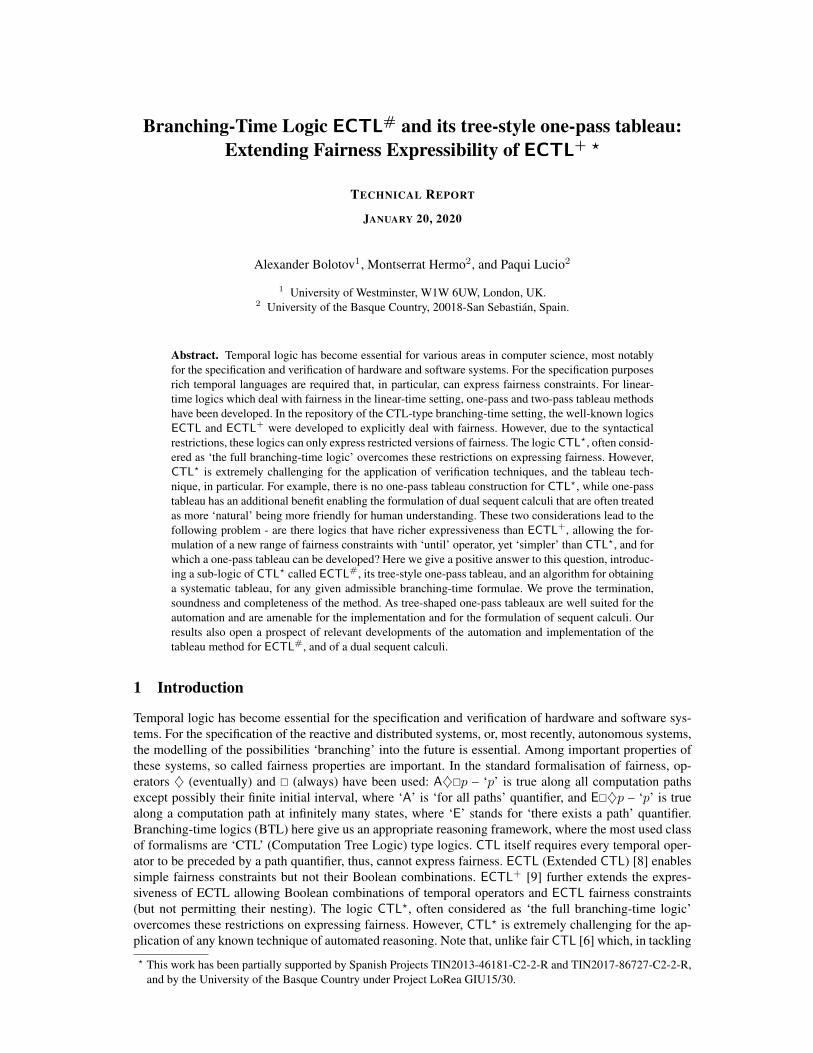
Definition 12 (Elementary Set of ECTL# State Formulae). A set of ECTL# state formulae is elemen-tary if and only if it is exclusively formed by literals and formulae of the form Q◦Π .

Proposition 13. Any set of ECTL# state formulae has a tableau T such that all its leaves are labelled byelementary sets of state formulae.

Proof. Repeatedly apply to every expandable node any applicable α-rule or β-rule.

Example 14. Figure 6 depicts a tableau with elementary leaves for A(◦q,�r),E(◦r, q U �¬p),E◦q. Re-call that A(◦q,�r) is an abbreviation of A(◦q,�(r ∨ �F)).

Definition 15 (Basic Path/State Formula and Uniform Set of Formulae). Every ECTL# path formulaof the type ◦σ, σ1 U (σ2∧♦σ3), σ1 U (�σ2), �(σ1∨�σ2), �(σ1 U σ2) is called basic. Every state formulaQΠ where Π is a set of basic-path formulae is also called basic. A set of state formulae Σ is uniform iffΣ is exclusively formed by literals and basic state formulae, and Σ contains at most one E-conjunctiveformula.

Proposition 16. Any set of ECTL# state formulae Σ has a tableau T such that labels of all its leavesare uniform sets of state formulae. Moreover, each open branch of T contains exactly one application of(Q◦).

Proof. Use Proposition 13 to construct a tableau with all its leaves labelled by elementary sets of formulae.Then apply the rule (Q◦), to any relevant node and, finally, repeatedly apply (to every expandable node)the rules (Eσ), (Aσ), (∧), and (∨).

Definition 17 (Uniform Tableaux). For any set Σ of ECTL# state formulae, the tableau for Σ providedby Proposition 16 is denoted Uniform_Tableau(Σ).

Fig. 6: A tableau whose leaves are elementary

Example 18. Constructing a uniform tableau for the set {A(◦q,�r),E(◦r, q U �¬p),E◦q)}, we first ob-tain the tableau in Figure 6. Then we apply the (Q◦) rule enlarging each of the four branches and producingthe following eight leaves, left to right (we refer to the node by its labels):

1. A(q,�r),E(r,�¬p) 2. A(q,�r),Eq 3. Aq,E(r,�¬p) 4. Aq,Eq

5. A(q,�r),E(r, q U �¬p) 6. A(q,�r),Eq 7. Aq,E(r, q U �¬p) 8. Aq,EqThen we apply the rules (Aσ) and (Eσ): the first branch is split into q, r,E�¬p and A�r, r,E�¬p; thesecond into q and A�r, q; the third yields only a child q, r,E�¬p; the fourth and the eighth yield only q;the fifth is split into two nodes q, r,E(q U �¬p) and A�r, r,E(q U �¬p); the sixth into q and A�r, q; andthe seventh yields the unique child q, r,E(q U �¬p).

β+-Rule Σ, β k S+Σ,βi

(1 ≤ i ≤ k)

(AU σ)+ Σ,A(σ1 U (σ2 ∧ ♦σ3), Π) 3

S+Σ,β1

= {σ2,A(♦σ3, Π)}S+Σ,β2

= {σ1,A(◦((σ1 ∧ (¬Σ ∨ ϕΠ))U (σ2 ∧ ♦σ3)), Π)}S+Σ,β3

= {AΠ}

(AU �)+ Σ,A(σ1 U �σ2, Π) 2S+Σ,β1

= {A(�σ2, Π)}S+Σ,β2

= {σ1,A(◦((σ1 ∧ (¬Σ ∨ ϕΠ ∨ σ2))U �σ2), Π)}

β+-Rule Σ, β k S+Σ,βi

(1 ≤ i ≤ k)

(EU σ�)+ Σ,EΠ 2n

S+Σ,β1

...

S+Σ,βi

=...

S+Σ,βn

{{σ2,E(♦σ3, Π

−i)} if πi = σ1 U (σ2 ∧ ♦σ3)

{E(�σ2, Π−i)} if πi = σ1 U �σ2

S+Σ,βn+1

...

S+Σ,β2i

=

{{σ1,E(◦((σ1 ∧ ¬Σ)U (σ2 ∧ ♦σ3)), Π

−i)} if πi = σ1 U (σ2 ∧ ♦σ3)

{σ1,E(◦((σ1 ∧ ¬Σ)U �σ2), Π−i)} if πi = σ1 U �σ2

...

S+Σ,β2n

Fig. 7: BETA-PLUS RULES. (Notation: σ, σi stand for state formulae, Σ is a (possibly empty) set of stateformulae,Π is a (possibly empty) set of basic-path formulae. Formula ϕΠ is defined in Def. 19. We denotebyΠU the set of all formulae inΠ that have the forms σ1 U (σ2∧♦σ3) and σ1 U �σ2.ΠU is enumeratedas {π1, . . . , πn} for n ≥ 1, and Π−i = Π \ {πi}.)

3.4 The Beta-plus Rules

In this subsection we extend our set of tableau rules with the new four rules named as β+-rules (Figure 7).These rules, similarly to β-rules, also split a branch, but this time into a number of branches dependingon the treated formula. The rules for A-disjunctive formulae apply to a label Σ, β, where β has the formA(π,Π), Π is a set of basic-path formulae, and π is either σ U (σ ∧ ♦σ) or σ U �σ. The rule (EU σ�)+for E-conjunctive formulae applies to a set Σ, β, where β has the form EΠ and Π is a set of basic-pathformulae that contains at least one formula σ U (σ ∧ ♦σ) or σ U �σ. The β+-rules are the only rules inour system that make use of the so-called context for forcing the eventualities to be satisfied as soon aspossible. The context is given by the sets Σ containing state formulae and Π containing path formulae.We name Σ the outer context and Π the inner context. The outer context is used by all the β+-rules. Theinner context is only needed to deal with formulae AΠ . The following formula, ϕΠ , introduced in Def. 19is used to manage the inner context Π in rules (AU σ)+ and (AU �)+.

Definition 19 (Formula ϕΠ for β+-rules on A-disjunctive formulae). Let Π be a set of basic pathformulae. We define the formula ϕΠ to be the following disjunction of state formulae (ϕΠ is F, if thebelow disjunction is empty):∨

�(σ1∨�σ2)∈Π

(σ1∨σ2) ∨∨

σ1 U �σ2∈Πσ2 ∨

∨�(σ1 U σ2)∈Π

E(♦σ2).

It is worth noting that each β+-rule, when applied to some formula of the form Q(σ1 U ϕ,Π) –whereϕ could be σ2 ∧ ♦σ3 or �σ2– generates one or more successors that contain a formula of the formQ(◦((σ1∧σ)U ϕ), Π) where σ depends on both the inner and the outer context, and is defined dependingon whether Q is E or A. We call (σ1 ∧ σ)U ϕ the next-step variant of σ U ϕ. Example 20 illustrates themain ideas behind the application of β+-rules (AU σ)+ and (AU σ).Example 20. The β+-rules (AU σ)+ applies to one selected formula with exactly one marked eventual-ity. Consequently, the (AU σ)-rule applies to all the eventualities (in the selected formula) except to themarked one.

τ(n0) : ¬b,A( aU b , pU q)

τ(n1) : ¬b, b

τ(n2) : ¬b, a,A(◦( (a ∧ b)U b ), pU q)

¬b, a, q ¬b, a, p,A(◦( (a ∧ b)U b ),◦(pU q)) ¬b, a,A◦( (a ∧ b)U b )

τ(n3) : ¬b,A( pU q )

¬b, q ¬b, p,

(AU σ)+

(AU σ)

(AU σ)+

Fig. 8: Application of (AU σ)+ and (AU σ) rules to {¬b,A(aU b, pU q)}

In Figure 8 the marked eventualities are in gray boxes. Assume aU b is the marked eventuality. Then, the(AU σ)+-rule can be applied to aU b) with outer context Σ = {¬b} and inner context, Π = {pU q}.According to Definition 19, ϕΠ is F. Therefore, S+

Σ,β1= {b}, S+

Σ,β3= {A(pU q)}, and S+

Σ,β2=

{a,A(◦((a ∧ b)U b), pU q)} respectively generate nodes n1, n2 and n3. In node n2, the (AU σ)-ruleis applied to pU q. That produces three new nodes. Regarding node n3, the marked eventuality disap-pears. Then, a new selection is made and pU q is marked. Consequently, (AU σ)+-rule is applied withouter contextΣ = {¬b}. The inner context is the empty set. Note that all leaves in Figure 8 are elementary.Hence, the construction of the tableau, would continue applying the next-state rule (Q◦).

3.5 Simplification Rules

A large set of simplification rules can be used to reduce the tableau construction. Here we only mentionthose that are essential for termination. First, to stop the growth of the subformula σ in the successive next-step variants (σ1 ∧ σ)U ϕ, we use trivial simplification rules such as ϕ ∧ ϕ −→ ϕ and ϕ ∨ ϕ −→ ϕ,as well as classical subsumptions rules. Second, to simplify the detection of equal labels (for looping intableau branches) we use the following (subsumption-based) rules:

(@E�U ) E(σ1 U σ2,�(σ1 U σ2), Π) −→ E(�(σ1 U σ2), Π).(@A�U ) If Π ′ ⊆ Π then A(σ1 U σ2, Π) ∧ A(�(σ1 U σ2), Π ′) −→ A(�(σ1 U σ2), Π ′).

Finally, to prevent the duplications of the original eventuality σ1 U σ2 and its successive new-stepvariants by rules (Q�U ) and (QU σ)+, and to ensure termination, we use the following (subsumption-based) simplification rules:

(@Aσ U ) σ2 ∧ A(σ1 U σ2, Π) −→ σ2.(@EU σ) E((σ1 ∧ σ)U ϕ, σ1 U ϕ,Π) −→ E((σ1 ∧ σ)U ϕ,Π)(@AU σ) If Π ′ ⊆ Π then A((σ1 ∧ σ)U ϕ,Π ′) ∧ A(σ1 U ϕ,Π) −→ A((σ1 ∧ σ)U ϕ,Π ′).

3.6 The role of ϕΠ in the Beta-plus Rules

Let us consider a set of formulae Φ = Σ,A(σ U ϕ,Π). A model, K, of Φ could satisfy A(σ U χ,Π)because each fullpath of K satisfies either σ U χ or some formula π ∈ Π . The next-step variant of σ U χis ◦(σ ∧ (¬Σ ∨ϕΠ))U χ), which makes ¬Σ or ϕΠ satisfiable before χ is satisfied. The former producesopen branches where χ is fulfilled as soon as possible, whereas the latter produces open branches thatsatisfy some of the π ∈ Π . Therefore, ϕΠ allows to generate a model from a branch in which σ U ϕ is notfulfilled, and some π ∈ Π is satisfied. Example 21 illustrates these ideas from the constructive view, i.ewhen we construct a tableau for a formula A(π1, . . . , πn).

τ(n1) : A(aU b,�c, r U �s,�(pU q))

τ(n2) : a,A(◦(α1︷ ︸︸ ︷

(a ∧ (c ∨ s ∨ E♦q))U b),�c, r U �s,�(pU q))

τ(n3) : A(α1,�c, (r U �s),�(pU q))

τ(n4) : a, (a ∧ (c ∨ s ∨ E♦q)),A(◦(α1),�c, r U �s,�(pU q))

τ(n5) : a, q, c, r, p,A(◦(α1),◦�c,◦(r U �s),◦(pU q)),A(◦(α1),◦�c,◦(r U �s),◦�(pU q))

τ(n6) : A(α1,�c, (r U �s),�(pU q))

(AU σ)+

(A�σ) + (AU �) + A�U ) + (AU σ) + (Q◦) + (@A�U )

(AU σ)+

(A�σ) + (AU �) + A�U ) + (AU σ) + (∧) + (∨)

(Q◦) + (@A�U )

Fig. 9: A branch of a tableau for A(aU b,�c, r U �s,�(pU q).

Example 21. Let Π = {�c, r U �s,�(pU q)}, and consider an application of the rule (AU σ)+ to theformula A(aU b, Π), where a, b, c, p, q, r, s ∈ Prop (see Figure 9). The outer context, namelyΣ, is emptyand the inner context is Π . Then ¬Σ is F and ϕΠ = c ∨ s ∨ E♦q. Hence, the second child, namelyS+Σ,β2

, raised by the application of (AU σ)+ is labelled by {a,A(◦α1, Π)} where α1 = (a ∧ ϕΠ)U b =(a∧ (c∨s∨E♦q)U b. Then, Uniform_Tableau applies the (corresponding) rules to �c, r U �s, �(pU q),and, finally, (Q◦) and the simplification rule (@ A�U ), obtaining the node n3. Now, one of the leavesraised by Uniform_Tableau is the fifth node; by applying here (Q◦) and (@A�U ) we obtain the last noden6 such that τ(n6) = τ(n3). This branch represents a model of the initial A-disjunctive formula whereboth disjuncts �(pU q) and �c are satisfied, though the other two disjuncts are not. Indeed, it representsthe model {a, c, r, p}, ({a, c, r, p, q})ω .

4 Systematic Tableau Construction

In this section we define an algorithm, Asys, that constructs a systematic tableau and illustrate its perfor-mance with some examples. Recall that due to the rule (Q◦), any open tableau should have a collection ofopen branches including all the (Q◦)-successors of any node labelled by an elementary set of formulae.These collections of branches are called bunches. Any open bunch of the systematic tableau, constructedby the algorithm Asys introduced in this section, enables the construction of a model for the initial set offormulae.

Algorithm 1 Systematic Tableau Construction1: procedure SYSTEMATIC_TABLEAU(Σ0) . where Σ0: set of state formulae2: if Σ0 is not uniform then T := Uniform_Tableau(Σ0)3: while T has at least one expandable node do4: . Invariant: Any expandable node of T is labelled by an uniform set5: Choose any node ` in T such that τ(`) is expandable6: Let Σ = τ(`) . Σ is uniform7: if there are not selectable formulae in ` then T := T [`←Uniform_Tableau(Σ)]8: else9: Eventuality_Selection(Σ)

10: Apply_β+-rule(Σ)11: Let k be the number of new leaves, `1, . . . , `k the new leaves and Σ1, . . . , Σk their labels12: for i = 1 .. k do13: if `i is expandable and Σi is not uniform then14: T := T [`i ←Uniform_Tableau(Σi)]15: return T

4.1 The Algorithm

The algorithm Asys constructs an expanded tableau (see Definition 41) for the given input. Asys appliedto the input Σ0, denoted as Asys(Σ0), returns a systematic tableau AsysΣ0

. Intuitively, ‘expanded’ means‘complete’ in the sense that any possible rule has been already applied at every node. Though the bestway to implement this algorithm is a depth-first construction, for clarity, we formulate it as a breadth-first construction of a collection of subtrees. The procedure Uniform_Tableau, in the above Algorithm1, was introduced in Definition 17 along with the notion of a uniform set of state formulae. The no-tation T1[` ← T2] stands for the tableau T1 where the expandable ` is substituted by the tableau T2.In particular, T [` ←Uniform_Tableau(Σ)] is the tableau T where the expandable ` is substituted bythe Uniform_Tableau(Σ). Next, we define the other two auxiliary procedures: Eventuality_Selectionand Apply_β+-rule, as well as the related concepts of selectable formula, non-expandable node andeventuality-covered branch. From now on any basic path formula that is either σ1 U (σ2∧♦σ3) or σ1 U �σ2or �(σ1 U σ2) is called an eventuality. It is worth noting that ◦π is not called an eventuality in this setting.

Definition 22 (Selectable Formula). A formula is selectable if it is a QΠ and Π contains at least oneeventuality.

Procedure Eventuality_Selection chooses formula QΠ and if Q = A then the procedure also marksone eventuality, according to the priorities of selection and marking in Definition 24. We denote by πUthe marked eventuality in the selected formula AΠ .

Procedure Apply_β+-rule(Σ) applies the corresponding rules depending on the selected formula QΠand on the marked eventuality in the case Q = A:

– If Q = A and σ1 U (σ2 ∧ ♦σ3) ∈ Π is the marked eventuality, then apply (AU σ)+– If Q = A and σ1 U �σ2 ∈ Π is the marked eventuality, then apply (AU �)+– If Q = A and �(σ1 U σ2) ∈ Π is the marked eventuality, then first apply the rule (A�U ) and then the

rule (AU σ)+ with the marked eventuality σ1 U σ2.– If Q = E and Π contains at least one σ1 U (σ2 ∧ ♦σ3) or one σ1 U �σ2 then apply (EU σ�)+

– If Q = E andΠ contains at least one �(σ1 U σ2) (but none σ1 U (σ2∧♦σ3) and none σ1 U �σ2), thenfirst apply the rule (E�U ) to every �(σ1 U σ2) and then the rule (EU σ�)+.

Each application of a β+-rule on the selected AΠ introduces a next-step variant of the marked eventualityand each application of a β+-rule on the selected EΠ introduces a next-step variant for each σ1 U (σ2 ∧♦σ3) and each σ1 U �σ2.

The call Eventuality_Selection(Σ) keeps the selection of the formula EΠ such that Π contains atleast one σ U (σ ∧ ♦σ) or σ U �σ, or keeps the selection of the formula AΠ ∈ Σ which contains thenext-step variant of the marked eventuality, or selects a new formula AΠ ∈ Σ that contains an eventuality.The latter can happen for three reasons. When formulae EΠ do not contain any σ U (σ∧♦σ) nor σ U �σ,or there is no marked eventuality in formulae AΠ , or when there is one, the node `, (Σ = τ(`)) is aloop-node (see Definition 25), and the branch from the root-node to ` is not eventuality-covered (seeDefinition 26). In this case, a new selection should be made because there are eventualities that havenever been marked but they should be. This way we introduce the term eventuality-covered. When abranch is eventuality-covered, its leaf is a loop-node and we are sure that, along the loop, at least someeventuality in each A-disjunctive formula and all eventualities in each E-conjunctive formula have beenfulfilled. Consequently, the branch is an expanded open branch (see Definition 41) and represents a path ina possible model. It is worth mentioning that the only requirement for a branch to be eventuality-coveredis to mark all necessary eventualities. The fact that formulae EΠ are kept selected whereas they containsome eventuality and formulae AΠ are kept selected where the next-step variant of the marked eventualityis kept marked ensures that every eventuality in EΠ and at least one in each AΠ is fulfilled.

When making the selection, priorities are used as stated in Definition 24. The idea behind priorities isthat a tableau branch represents a path in a cyclic Kripke structure that is a possible model for the inputformula. Therefore, it consists of a (possibly empty) initial sequence of states followed by a looping-sequence. Selectable formulae are classified into two sets - those of the highest priority and those of thelowest priority. The non-looping initial sequence is the first part of the model, hence we firstly selectformulae AΠ where Π is exclusively formed by formulae of the form σ1 U (σ2 ∧♦σ3) and formulae EΠwhere Π contains at least one eventuality of the form σ1 U (σ2 ∧♦σ3) or σ1 U �σ2. These are the highestpriority formulae, which cannot produce a loop. When one of the former formulae AΠ is selected, oneof the σ1 U (σ2 ∧ ♦σ3) is marked, namely π. By means of the rule (AU σ)+, in a finite number of steps,either the branch close or π is either fulfilled (note that in the first branch A(♦σ3, Π) is also of the highestpriority) or deleted (the third branch of (AU σ)+). In any case the original formulae AΠ disappears.When one of the latter formulae EΠ is selected, the successive applications of the rule (EU σ�)+ ensure(excluding the case when the branch closes) the fulfillment of all σ1 U (σ2 ∧ ♦σ3) or σ1 U �σ2 in a finitenumber of states. Note that E(♦σ3, Π) is also of the highest priority. Once such formulae are fulfilled,all formulae σ1 U (σ2 ∧ ♦σ3) have disappeared from the E-conjunctive formula, whereas �σ2 remains inthe conjunction for all σ1 U �σ2 ∈ Π . Hence, the residual EΠ ′ is of the lowest-priority. On the contrary,the lowest priority formulae could produce a loop. They are formulae AΠ where Π contains at least oneσ1 U �σ2 or �(σ1 U σ2) and formulae EΠ where Π contains at least one �(σ1 U σ2) (but are not of thehighest priority). They could produces a loop in a finite number of steps, since the subformulae startingby � remains forever in the E-disjunctive formulae, whereas in the A-disjunctive formulae they can eitherremain or disappear. In the latter case, the residual A-disjunctive formulae could become non-selectable.It is easy to see that non-selectable formulae necessarily produce a loop.

Example 23. Consider Σ0 = {A(aU b, bU c),E(pU q,�(r U s)),A�(cU d),¬b,A�e}. The first two for-mulae have the highest-priority, the third has the lowest priority, and the the last two are non-selectable.Suppose that we select A(aU b, bU c) and mark aU b, since ¬b ∈ Σ0, the left-most open branch of rule(AU σ)+ contains a,A(◦((a ∧ ¬Σ′0)U b), bU c) where Σ′0 = Σ0 \ {A(aU b, bU c)}. After applying thecorresponding α and β rules to the remaining formulae, the first stage s0 (the first state of the model)contains the atoms {a, q, s, d, e}. Then, by the next-step rule (Q◦), the first node of the second stage s1 isΣ1 = {A((a ∧ ¬Σ′0)U b, bU c),E�(r U s),A�(cU d),A�e} where the first formula is kept selected andthe first eventuality is kept marked. Note that the second formula has now the lowest priority. Then weapply (AU σ)+ to the first formulae and the corresponding α and β rules to the remaining formulae inΣ1, generating the set of atoms in the left-most branch are {b, s, d, e}. Then, by the next-step rule (Q◦),the first node of the third stage s2 is Σ2 = {E�(r U s),A�(cU d),A�e} where the first two formulas

are of the lowest priority and the third is non-selectable. By selecting the first formula, the atoms in thestages s2 (of the left-most branch) are {s, d, e} and the new uniform set at the first node of the followingstage is Σ3 = Σ2. However, A�(cU d) has not been selected inside the loop, hence we produce one stagemore, s3, with atoms {s, d, e}. Then, by (Q◦), we obtain Σ4 = Σ2 and the branch is eventuality-covered.Therefore, we have a model for Σ0 is s0, s1〈s2, s3〉ω .

Definition 24 (Priorities for Eventuality Selection). The selectable formulae of the highest priority forEventuality_Selection are the formulae of the following two forms:

– AΠ where Π is exclusively formed by formulae of the form σ1 U (σ2 ∧ ♦σ3).– EΠ where Π contains at least one eventuality of the form σ1 U (σ2 ∧ ♦σ3) or σ1 U �σ2.

Consequently, the (selectable) formulae of the lowest priority are the formulae of the following two forms:

– AΠ where Π contains at least one σ1 U �σ2 or �(σ1 U σ2).– EΠ where Π does not contain any σ1 U (σ2 ∧ ♦σ3) nor σ1 U �σ2, and Π contains at least one�(σ1 U σ2).

Once all the highest priority formulae have been selected in a branch, the only selectable formulaeare the lowest priority formulae. At this point, the objective is to get a loop-node that makes the brancheventuality-covered.

Definition 25 (Loop-node). Let b be a tableau branch and ni ∈ b (0 ≤ i). Then ni is a loop-node if thereexists nj ∈ b (0 ≤ j < i) and τ(ni) = τ(nj). We say that nj is a companion node of ni.

Definition 26 (Eventuality-covered Branch). A tableau branch b = n0, n1, ..., ni is eventuality-coveredif ni is a loop-node, with a companion node nj (0 ≤ j < i), both labelled by a uniform set Σ of non-selectable and the lowest priority formulae such that every selectable formula QΠ ∈ τ(ni) is selected insome node nk (j ≤ k < i) and for every selected AΠ exactly one eventuality in Π is marked in somenode nk such that j ≤ k < i.

The procedure Eventuality_Selection performs in some fair way that ensures that any open branch willever be eventuality-covered.

Definition 27 (Non-expandable Node). A node n is non-expandable, if τ(n) = Σ⊥ or n is a loop-nodeof branch b which is eventuality-covered. Otherwise, n is expandable.

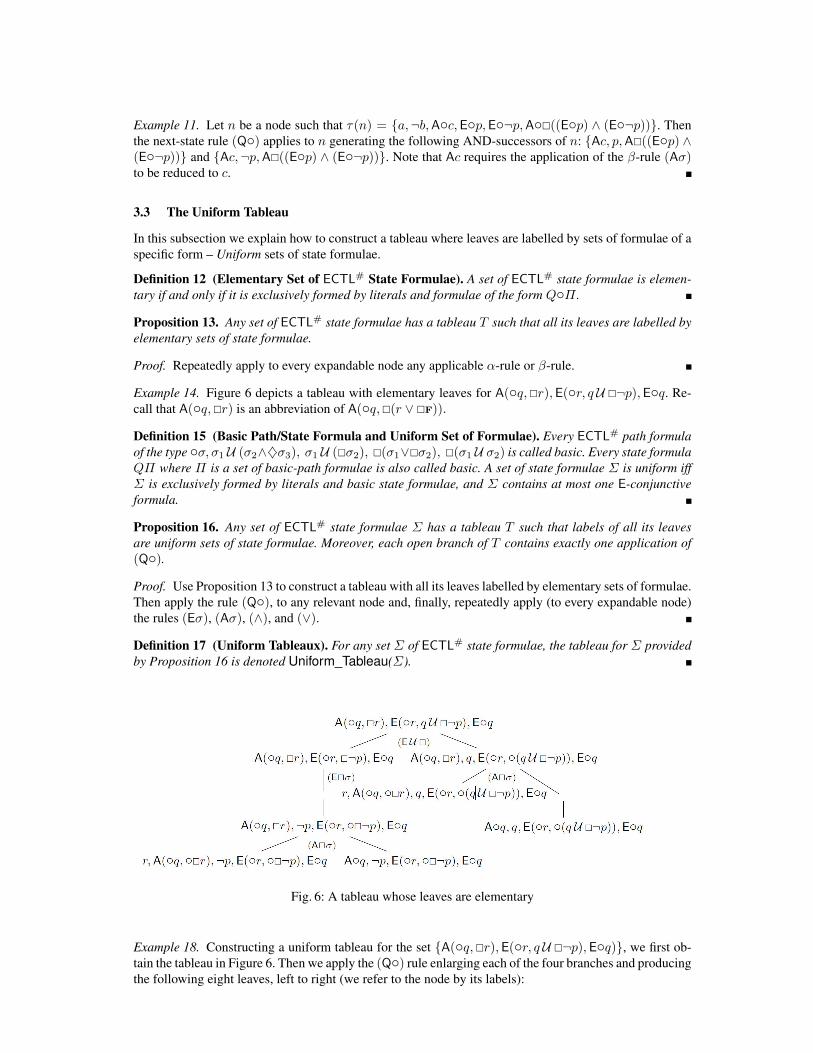
Consequently, an expandable node is either a node that is not a loop-node or a loop-node whose branchis not eventuality-covered. It is worth noting that a formula of the lowest priority could be selected morethan once in a branch because the loop-node could change along the branch. In the following Example 28,we illustrate this issue.Example 28. Figure 10 shows a branch in the systematic tableau forΣ0 = {A(pU ¬p,�p),A�(aU E�c)}where, for readability, the marked eventualities are in gray boxes. The call Eventuality_Selection(Σ0) se-lects the formula A(pU ¬p,�p) in n1. Generating n2, when we apply the (AU σ)+ rule to A(pU ¬p,�p),the outer context is A�(aU E�c) and the inner context is p. Hence, in the S+

Σ,β2branch, the next-step

variant of pU ¬p is p ∧ (¬(A�(aU E�c) ∨ p))U ¬p. By classical subsumption (included in our simplifi-cation rules), p ∧ (¬(A�(aU E�c) ∨ p) −→ p, hence the next-step variant is pU ¬p, and the formulaA(◦(pU ¬p),�p) is added to the current stage. Then, applying (A�σ) to A(◦(pU ¬p),�p), (A�U ) to(A�(aU E�c), and (AU σ) to A(aU E�c), the node n2 is obtained. After the application of (Q◦) and(@ A�U ), n3 is obtained. Node n3 is a loop-node whose companion node is n1 (τ(n3) = τ(n1)).However, the branch is not eventually-covered since the eventuality aU E�c is not selected inside theloop. Therefore, we obtain n4 by the call Eventuality_ Selection((τ(n3)) which selects A(aU E�c).After applying the (AU σ)+ rule to A(aU E�c) (once the (A�U ) rule is applied), the branch S+

Σ,β1

expands to n5. After that, Uniform_Tableau gets one expandable node labelled by the uniform set{E�c,A(pU ¬p,�p),A�(aU E�c)} as represented in n6. The call Eventuality_Selection((τ(n6)) se-lects again the formula A(pU ¬p,�p). Now, the outer context is {E�c,A�(aU E�c)} and the inner contextis p. Hence, by subsumption, p∧ (¬(E�c)∨¬(A�(aU E�c))∨ p) −→ p. Hence, the S+

Σ,β2branch con-

tains again the next-step variant pU ¬p in n7. Then, expanding the Uniform_Tableau we obtain n8 which

τ(n1) : A( pU ¬p ,�p),A�(aU E�c)

τ(n2) : p, a,A(◦( pU ¬p ),◦�p),A◦(aU E�c),A◦�(aU E�c)

τ(n3) : A( pU ¬p ,�p),A�(aU E�c)

τ(n4) A(pU ¬p,�p),A�( aU E�c )

τ(n5) : E�c,A(pU ¬p,�p),A◦�(aU E�c)

τ(n6) : E�c,A( pU ¬p ,�p),A�(aU E�c)

τ(n7) : p,E�c,A(◦( pU ¬p ),�p),A�(aU E�c)

τ(n8) : p, c,E◦�c,A(◦( pU ¬p ),◦�p),A◦�(aU E�c)

τ(n9) : E�c,A( pU ¬p ,�p),A�(aU E�c)

τ(n10) : E�c,A(pU ¬p,�p),A�( aU E�c )

τ(n11) : p, c,E◦�c,A(◦(pU ¬p),◦�p),A◦�(aU E�c)

τ(n12) : E�c,A(pU ¬p,�p),A�(aU E�c)

(AU σ)+ + (A�σ) + (A�U ) + (AU σ)

(Q◦) + (@A�U )

(not eventuality covered)

(A�U ) + (AU σ)+

(AU σ) + (A�σ) + (E�σ) + (Q◦)

(AU σ)+

(A�σ) + (A�U ) + (AU σ) + (E�σ)

(Q◦)

(not eventuality covered)

(A�U ) + (AU σ)+ + (AU σ) + (A�σ) + (E�σ)

(Q◦)

Fig. 10: A branch in the systematic tableau for A(pU ¬p,�p),A�(aU E�c)

is an expandable loop-node because τ(n8) = τ(n6). However, the branch is not yet eventually-coveredsince aU E�c has not been marked inside the loop. Then, the selected formula in n9 is A(aU E�c). Fi-nally, Uniform_Tableau obtains a non-expandable loop-node, thus the given branch is eventually-covered- depicted in Figure 10 it represents {p, a}({p, c})w, which is a model of Σ0. However, considering allthe nodes in the branch, one would realize that the model represented is {p, a}{p, c}({p, a, c}{p, c})w.

Definition 29 (Bunch in a Tableau, Closed Bunch and Tableau). A bunch b is a collection of branchesthat is maximal with respect to (Q◦)-successor, i.e. every (Q◦)-successor of any node in b is also in b. Abunch is closed iff at least one of its branches is closed, otherwise it is open. A tableau is closed iff allits bunches are closed.

Therefore, any open tableau has at least one open bunch, formed by one or more open branches. Tocomplete, this section we provide two examples: a closed tableau and an open tableau. We mark eventual-ities in gray boxes and use large circles to represent the generation of AND-nodes or bunches.

4.2 Examples

In this Subsection we provide some examples of systematic tableaux. For readability, the marked eventu-alities are in gray boxes. Big circles are used to represent AND-nodes or bunches. Whenever a bunch hasa unique successor, we omit the big circle in the edge before the (Q◦)-successor.

A( TU ¬p ,�p)

¬p

∅

∅

A(◦( pU ¬p ),�p)

A◦( pU ¬p )

A( pU ¬p )

¬p

∅

∅

p,A◦( (F ∧ p)U ¬p )

A( (F ∧ p)U ¬p )

¬p

∅

∅

(F ∧ p),A◦( (F ∧ p)U ¬p )

F, p, . . .

p,A(◦( pU ¬p ),◦�p)

A( pU ¬p ,�p)

¬p

∅

∅

p,A(◦( pU ¬p ),�p)

p,A◦( pU ¬p )

A( pU ¬p )

p,A(◦( pU ¬p ),◦�p)

A( pU ¬p ,�p)

A(�p)

p,A(◦�p)

A(�p)

A(�p)

p,A(◦�p)

A(�p)

(AU σ)+

(Q◦)

(Q◦)(A�σ)

(Q◦)

T

(Q◦)

(Q◦)(Q◦)

(AU σ)+

(Q◦)

(Q◦)

(∧)

⊗

(Q◦)

(AU σ)+

(Q◦)

(Q◦)(A�σ)

(Q◦)

T

(Q◦)

(A�σ)

(Q◦)

(A�σ)

(Q◦)

Fig. 11: An open tableau for A(TU ¬p,�p)

Example 30. In Figure 11 we depict an open tableaux for A(TU ¬p,�p) or equivalently A(♦¬p,�p). Infact, the tableau has only one closed branch –the fourth branch from the left. The remaining branchesare finished by a loop-node. There are only three different labels of loop-nodes (that are repeated in

different branches): the empty set of formulae, the singleton containing the potentially-cycling formulaA(pU ¬p,�p), and the singleton containing the cycling formula A�p.

A( TU p ),E�¬p

p,E�¬p

p,¬p,E◦�¬p

A◦( (A♦p)U p ),E�¬p

A◦( (A♦p)U p ),¬p,E◦�¬p

A( (A♦p)U p ),E�¬p

p,E�¬p

p,¬p,E◦�¬p

A♦p,A◦( (A♦p)U p ),E�¬p

(AU σ)+

(E�σ)

⊗

(E�σ)

(Q◦)

(AU σ)+

(E�σ)

⊗

⊗

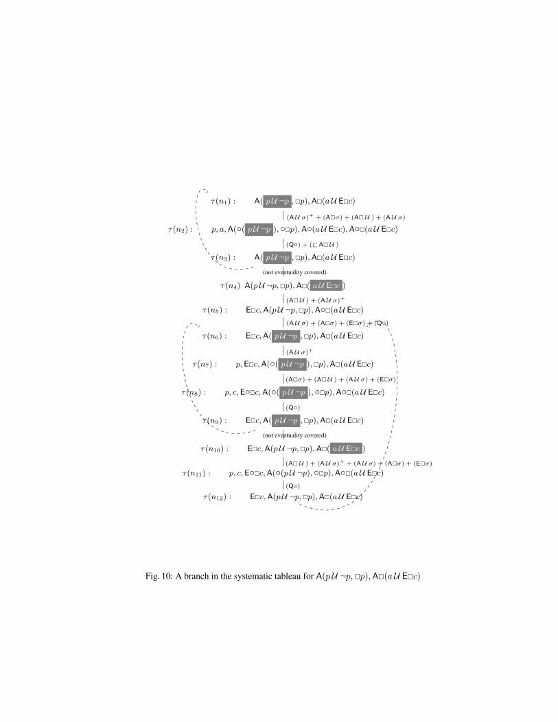
Fig. 12: A closed tableau for A(TU p),E�¬p.

Example 31. In Figure 12 we depict a closed tableau for A(TU p),E�¬p. Note that, in the two applica-tions of the rule (AU σ)+, the inner context is empty and the outer context is E�¬p whose negation innnf is A♦p. Henceforth, the rightmost leaf in Figure 12 is the result of simplifying the selected formulafrom A◦(((A♦p) ∧ (A♦p))U p) to A◦((A♦p)U p). This right-most branch is closed because A♦p is thenegation normal form of E�¬p.

p,A�(E◦p ∧ E◦¬p),A( ♦¬p ,�p)

p,A�(E◦p ∧ E◦¬p),A(◦( (¬p ∨ E♦(A◦¬p ∨ A◦p) ∨ p)U ¬p ,�p)

p,A�(E◦p ∧ E◦¬p),A( ♦¬p ,�p) ¬p,A�(E◦p ∧ E◦¬p)

p,A�(E◦p ∧ E◦¬p)

p,A�(E◦p ∧ E◦¬p) ¬p,A�(E◦p ∧ E◦¬p)

¬p,A�(E◦p ∧ E◦¬p)

(AU σ)+

Uniform_Tableau (including (Q◦)) + Simplification

Uniform_Tableau (including (Q◦))

Uniform_Tableau (including (Q◦))

p

¬p

p

Fig. 13: Open bunch in the tableau for p,A�(E◦p ∧ E◦¬p),A(♦¬p,�p).

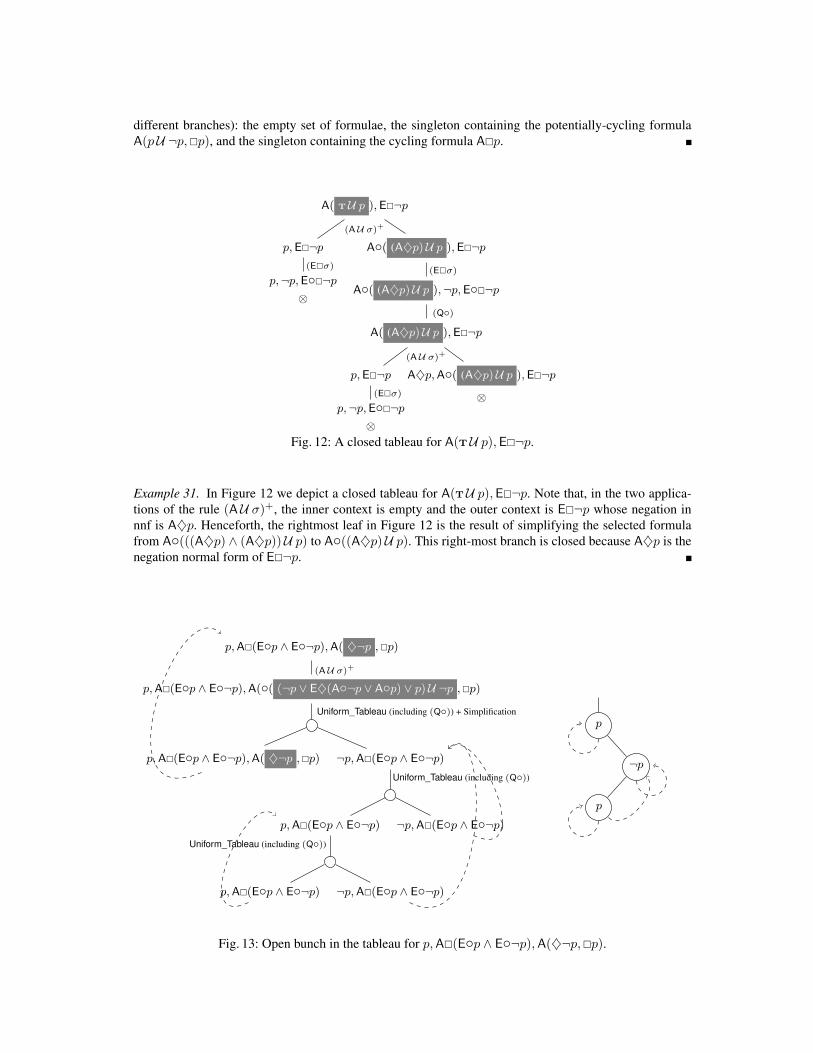
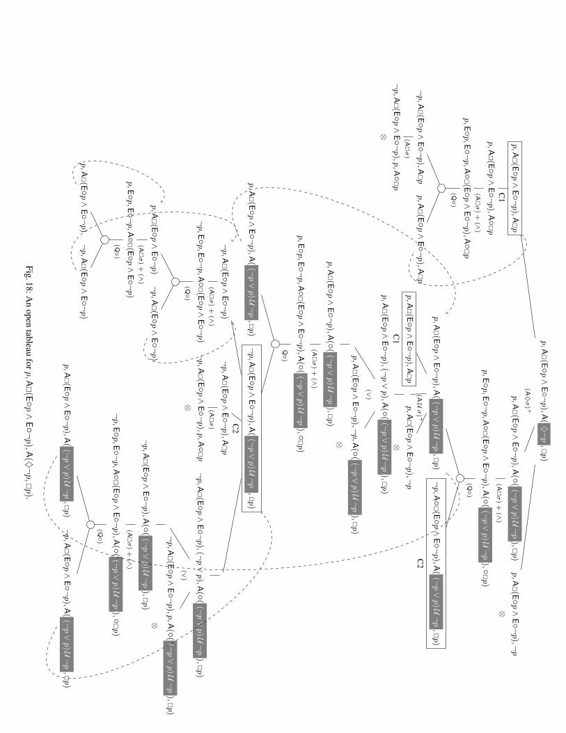
Example 32. On the left of Figure 13 we depict a representative open bunch of a tableau for the set offormulae:

{p,A�(E◦p ∧ E◦¬p),A(♦¬p,�p)}.In this example, we apply at once the Uniform_Tableau procedure subsequently choosing one of theleaves produced. Note that, for each node, we draw only one of the OR-children, but all the AND-children.The whole tableau, using the derived rules introduced in Section 5, is depicted in Figure 18, where all therule applications are detailed. It is explained in Example 35.Note that, for each node, we draw only one of the OR-children, but all the AND-children. In the markedeventuality, ¬p ∨ E♦(A◦¬p) comes from the negation of the outer context, and the disjunct p from theinner context. By ‘Simplification’ (¬p∨E♦(A◦¬p∨A◦p)∨p) is reduced to T (in the left-hand children).In the right-hand node, ¬p subsumes A((. . . )U ¬p,�p). This open bunch represents the model (of theinput set of formulae) that we depict in the right-hand of Figure 13. Since A(♦¬p,�p) is a valid formula,it is easy to see that it is a model of p,A�(E◦p ∧ E◦¬p).

5 Derived Rules and Examples

In this section we introduce some derived rules and give some examples of tableaux.

α_Rule α Sα

(A♦�) A(♦�σ,Π) {σ,A(◦♦�σ,Π)}(E�♦) E(�♦σ), Π) {E(♦σ,◦�♦σ,Π)}(A�♦) A(�♦σ,Π) {A(♦σ,Π),A(◦�♦σ,Π)}

β_Rule β k Sβi(1 ≤ i ≤ k)

(E♦σ) E(♦(σ1 ∧ ♦σ2), Π) 2Sβ1

= {σ1,E(♦σ2, Π}Sβ2

= {E(◦♦(σ1 ∧ ♦σ2), Π)}

(E♦�) E(♦�σ,Π) 2Sβ1

= {E(�σ,Π)}Sβ2

= {E(◦♦�σ,Π)}

(A♦σ) A(♦(σ1 ∧ ♦σ2), Π) 3

Sβ1= {σ1,A(♦σ2, Π)}

Sβ2= {A(◦♦(σ1 ∧ ♦σ2), Π)}

Sβ3 = {AΠ}

β+-Rule Σ, β k S+Σ,βi

(1 ≤ i ≤ k)

(A♦σ)+ Σ,A(♦(σ1 ∧ ♦σ2), Π) 3

S+Σ,β1

= {σ1,A(♦σ2, Π)}S+Σ,β2

= {A(◦((¬Σ ∨ ϕΠ)U (σ1 ∧ ♦σ2)), Π)}S+Σ,β3

= {AΠ}

(A♦�)+ Σ,A(♦�σ,Π) 2S+Σ,β1

= {A(�σ,Π)}S+Σ,β2

= {A(◦((¬Σ ∨ ϕΠ ∨ σ)U �σ), Π)}

β+-Rule Σ, β k S+Σ,βi

(1 ≤ i ≤ k)

(E♦σ�)+ Σ,EΠ 2n

S+Σ,β1

...

S+Σ,βi

=...

S+Σ,βn

{{σ1,E(♦σ2, Π

−i)} if πi = ♦(σ1 ∧ ♦σ2)

{E(�σ,Π−i)} if πi = ♦�σ

S+Σ,βn+1

...

S+Σ,β2i

=

{{E(◦((¬Σ)U (σ1 ∧ ♦σ2)), Π

−i)} if πi = ♦(σ1 ∧ ♦σ2)

{E(◦((¬Σ)U �σ), Π−i)} if πi = ♦�σ...

S+Σ,β2n

Fig. 14: DERIVED RULES. (Notation: σ, σi stand for state formulae, Σ is a (possibly empty) set of stateformulae,Π is a (possibly empty) set of basic-path formulae. Formula ϕΠ is defined in Def. 19. We denotebyΠU the set of all formulae inΠ that have the forms σ1 U (σ2∧♦σ3) and σ1 U �σ2.ΠU is enumeratedas {π1, . . . , πn} for n ≥ 1, and Π−i = Π \ {πi}.)

We introduce some trivially correct rules that just allow us to make tableaux shorter and easier to un-derstand.

First, we introduce a refinement of the rules β+-rules. It is easy to see, that instead of ¬Σ in theserules we can write ¬Σ′ where

Σ′ = Σ \ {A(π1, . . . , πn) | A(π1, . . . , πn) ∈ Σ and for all i : πi is �ϕ or ◦�ϕ}.This refinement just prevents to generate (at each application of a β+-rule) one closed branch for eachformula of the form A(π1, . . . , πn) that belongs to Σ. The idea is that the formula

A([◦]�ϕ1, . . . , [◦]�ϕn)is invariantly preserved from one stage to another (because of the rules (A�σ), (A�U ) and (Q◦)), so thenext application of the beta-plus rule to the selected eventuality produce a branch containing

¬A([◦]�ϕ1, . . . , [◦]�ϕn).However, this branch is closed at once because it also contains A([◦]�ϕ1, . . . , [◦]�ϕn). Interestingly,the formulae of the form E(�ϕ1, . . . ,�ϕn) has not the same property. Consequently, in this section, anyapplication of a β+-rule will get ¬Σ′ instead of ¬Σ. Of course, for empty Σ there is no difference, weget F in both options.

Second, in Figure 14, we introduce the derived rules for the temporal operator ♦, using its definitionin terms of U : ♦ϕ ≡ TU ϕ.

Third, subsumption is also very useful to make shorter (but equivalent) nodes in tableaux. In theexamples we will develop in this section, we use the following subsumption-based equivalences alongwith the simplification rules of Subsection 3.5. We use them just in the application of the rule (Q◦)(implicitly), when possible. Derived from the simplification rules in Subsection 3.5:

(@E�♦) E(♦σ,�♦σ), Π) ≡ E(�♦σ,Π).(@A�♦) If Π ′ ⊆ Π then A(♦σ′, Π) ∧ A(�♦σ′, Π ′) ≡ A(�♦σ′, Π ′).(@Aσ♦) σ ∧ A(♦σ,Π) ≡ σ.(@E♦σ) E(σ U ϕ,♦ϕ,Π) ≡ E(σ U ϕ,Π)(@A♦σ) If Π ′ ⊆ Π then A(σ U ϕ,Π ′) ∧ A(♦ϕ,Π) ≡ A(σ U ϕ,Π ′).

Other useful simplification rules are:

(@AΠ) AΠ ∧ AΠ ′ ≡ AΠ ′ if Π ′ ⊆ Π .(@EΠ) EΠ ∧ EΠ ′ ≡ EΠ if Π ′ ⊆ Π .

In the rest of this section we provide some examples of systematic tableau constructions. They areexplained in Examples 33, 34 and 35. As in the previous examples, the marked eventualities are in grayboxes; big circles are used to represent AND-nodes or bunches; and we omit the big circle in the edgebefore the (Q◦)-successor,whenever a bunch has a unique successor.

A( pU ¬p )

¬p

∅

∅

p,A(◦( (p ∧ F)U ¬p) )

A( (p ∧ F)U ¬p )

¬p

∅

∅

(p ∧ F),A(◦( (p ∧ F)U ¬p )

p,F,A(◦( (p ∧ F)U ¬p ))

(AU σ)+

(Q◦)

(Q◦)

(Q◦)

(AU σ)+

(Q◦)

(Q◦)

(∧)

⊗

Fig. 15: An open tableau for A(pU ¬p).

A( pU ¬p ,�p)

¬p

∅

∅

p,A(◦( pU ¬p ),�p)

p,A(◦( pU ¬p ))

A( pU ¬p )

p,A(◦( pU ¬p ),◦�p)

A( pU ¬p ,�p)

A(�p)

p,A(◦�p)

A(�p)

(AU σ)+

(Q◦)

(Q◦)

(A�σ)

(Q◦)

(Fig 15)

(Q◦)

(A�σ)

(Q◦)

Fig. 16: An open tableau for A(pU ¬p,�p)

Example 33. In Figure 15 we depict an open tableau for the singleton {A(pU ¬p)} that is a sub-tableau ofthe tableau in Figure 16. In the first tableau, both the outer and the inner context are empty, for the markedeventuality. However, in Figure 16, the eventuality marked in the root has empty outer context, but theinner context is �p, hence the formula in the left-hand side of the U is p as simplification of T ∧ (F ∨ p).Note that the central open branch represents a model of �p.

A ♦p ,E�¬q,A�(¬p ∨ q)

p,E�¬q,A�(¬p ∨ q)

p,A�(¬p ∨ q),¬q,E◦�¬q

p, (¬p ∨ q),A◦�(¬p ∨ q),¬q,E◦�¬q

p,¬p,A◦�(¬p ∨ q),¬q,E◦�¬q p, q,A◦�(¬p ∨ q),¬q,E◦�¬q

E�¬q,A�(¬p ∨ q),A◦( (A♦q)U p )

¬q,E◦�¬q,A�(¬p ∨ q),A◦( (A♦q)U p )

¬q,E◦�¬q, (¬p ∨ q),A◦�(¬p ∨ q),A◦( (A♦q)U p )

¬q,E◦�¬q,¬p,A◦�(¬p ∨ q),A◦( (A♦q)U p )

E�¬q,A�(¬p ∨ q),A( (A♦q)U p )

E�¬q,A�(¬p ∨ q), p

¬q,E◦�¬q,A�(¬p ∨ q), p

¬q,E◦�¬q, (¬p ∨ q),A◦�(¬p ∨ q), p

¬q,E◦�¬q,¬p,A◦�(¬p ∨ q), p ¬q,E◦�¬q, q,A◦�(¬p ∨ q), p

E�¬q,A�(¬p ∨ q),A♦q,A◦( (A♦q)U p )

¬q,E◦�¬q, q,A◦�(¬p ∨ q),A◦( (A♦q)U p )

(A♦σ)+

(E�σ)

(A�σ)

(∨)

⊗ ⊗

(E�σ)

(A�σ)

(∨)

(Q◦)

(AU σ)+

(E�σ)

(A�σ)

(∨)

⊗ ⊗

⊗

⊗

Fig. 17: A closed tableau for A♦p,E�¬q,A�(¬p ∨ q).

Example 34. In Figure 17 we depict a closed tableau that proves the unsatisfiability of the set of formulae:A♦p,E�¬q,A�(¬p ∨ q). For the selected eventuality the inner context is empty, but the outer contextis formed by two formulas: E�¬q whose negation in normal form is A♦q and the formula A�(¬p ∨ q)which, as explained above, is excluded from the negation of the context, because the branch it generatesis necessarily closed. Note that the unique application of (Q◦) enlarge the branch with a unique child forthe only E-formula.

Example 35. In Figure 18 we show the open tableau for p,A�(E◦p ∧ E◦¬p),A(♦¬p,�p).We have named as C1 and C2 two sub-tableaux that are repeated.For the eventuality marked in the root none of both context is empty, thought the formula A�(E◦p∧E◦¬p)is excluded in the negated outer context, as explained above. Though the formula¬p∨p could be simplifiedas T, however we keep it unsimplified in this example for illustrating that not all simplification are crucialfor termination. In fact, this is not, though many trivial simplifications are very useful for efficient.Note that the left-most bunch (of two branches) is closed because its left-most branch is closed, though itsright branch is open.One of the open bunches of this tableau (and the model its represents) is given in Figure 13 and explainedin Example 32.

p,A�(E◦

p∧E◦¬

p),A

(♦¬p,�p)

p,A�(E◦

p∧E◦¬

p),A

�p

p,A�(E◦

p∧E◦¬

p),A◦

�p

p,E◦

p,E◦¬

p,A◦

�(E◦

p∧E◦¬

p),A◦

�p

¬p,A�(E◦

p∧E◦¬

p),A

�p

¬p,A�(E◦

p∧E◦¬

p),p

,A◦�p

p,A�(E◦

p∧E◦¬

p),A

�p

p,A�(E◦

p∧E◦¬

p),A

(◦((¬p∨p)U¬p),�p)

p,E◦

p,E◦¬

p,A◦

�(E◦

p∧E◦¬

p),A

(◦((¬p∨p)U¬p),◦�p)

p,A�(E◦

p∧E◦¬

p),A

((¬p∨p)U¬p,�p)

p,A�(E◦

p∧E◦¬

p),A

�p

p,A�(E◦

p∧E◦¬

p),(¬

p∨p),A

(◦((¬p∨p)U¬p),�p)

p,A�(E◦

p∧E◦¬

p),A

(◦((¬p∨p)U¬p),�p)

p,E◦

p,E◦¬

p,A◦

�(E◦

p∧E◦¬

p),A

(◦((¬p∨p)U¬p),◦�p)

p,A�(E◦

p∧E◦¬

p),A

((¬p∨p)U¬p,�p)¬p,A�(E◦

p∧E◦¬

p),A

((¬p∨p)U¬p,�p)

¬p,A�(E◦

p∧E◦¬

p)

¬p,E◦

p,E◦¬

p,A◦

�(E◦

p∧E◦¬

p)

p,A�(E◦

p∧E◦¬

p)

p,E◦

p,E◦¬

p,A◦

�(E◦

p∧E◦¬

p)

p,A�(E◦

p∧E◦¬

p)¬p,A�(E◦

p∧E◦¬

p)

¬p,A�(E◦

p∧E◦¬

p) ¬p,A�(E◦

p∧E◦¬

p),A

�p

¬p,A�(E◦

p∧E◦¬

p),p

,A◦�p¬p,A�(E◦

p∧E◦¬

p),(¬

p∨p),A

(◦((¬p∨p)U¬p),�p)

¬p,A�(E◦

p∧E◦¬

p),A

(◦((¬p∨p)U¬p),�p)

¬p,E◦

p,E◦¬

p,A◦

�(E◦

p∧E◦¬

p),A

(◦((¬p∨p)U¬p),◦�p)

p,A�(E◦

p∧E◦¬

p),A

((¬p∨p)U¬p,�p)¬p,A�(E◦

p∧E◦¬

p),A

((¬p∨p)U¬p,�p)

¬p,A�(E◦

p∧E◦¬

p),p

,A(◦

((¬p∨p)U¬p),�p)

p,A�(E◦

p∧E◦¬

p),¬

p,A

(◦((¬p∨p)U¬p),�p)

p,A�(E◦

p∧E◦¬

p),¬

p ¬p,A◦

�(E◦

p∧E◦¬

p),A

((¬p∨p)U¬p,�p)

p,A�(E◦

p∧E◦¬

p),¬

p

(A♦σ)+

C1

(A�σ)+

(∧)

(Q◦)

(A�σ)

⊗

(A�σ)+

(∧)

(Q◦)

(AUσ)+

C1

(∨)

(A�σ)+

(∧)

Q◦)

C2

(A�σ)+

(∧)

(Q◦)

(A�σ)+

(∧)

(Q◦)

(A�σ)

⊗(∨

)

(A�σ)+

(∧)

(Q◦)

⊗

⊗ ⊗

C2

⊗

Fig.18:An

opentableau

forp,A�(E◦

p∧E◦¬

p),A

(♦¬p,�p).

6 Soundness

To prove the soundness of our tableau method (Theorem 38) we show that every tableau rule preservessatisfiability (Lemma 37). To prove the latter we essentially use the limit closure property, ensuring thatthe satisfiability of the negated inner context is preserved from segments of a limit path to the limit pathitself (Proposition 36). The use of ϕΠ (Definition 19) is crucial here.

Proposition 36 (Preservation of the Negated Inner Context ). Let Π be any set of basic path for-mulae and let ϕΠ be as in Definition 19. Let K be a Kripke structure, x1 ∈ fullpaths(K) such thatK, x1, 0 |= ¬Π . Let y = x≤i11 x≤i22 · · ·x≤ikk · · · be a limit path in fullpaths(K), for some i1 > 0 and somex≤i22 · · ·x≤ikk · · · . Then K, y, 0 |= ¬π holds for all π ∈ Π , provided that the following two conditionshold for all n ≥ 1:

(a) K, x≤i11 x≤i22 · · ·xn, j |= ¬σ2 for all σ1 U (σ2 ∧ ♦σ3) ∈ Π and all j ∈ {0..in}, and(b) K, x≤i11 x≤i22 · · ·x≤inn , in |= ¬ϕΠ .

Proof. We check the four cases of a basic path formula π ∈ Π . If π is of the form ◦σ, thenK, y, 0 |= ¬◦σbecauseK, y, 0 |= ¬π and i1 > 0. If π is of the form σ1 U (σ2∧♦σ3), then property (a) ensures that everystate in y satisfies ¬σ2. Therefore, ¬(σ1 U (σ2∧♦σ3)) is satisfied along the limit path y. For the remainingthree cases, on the basis of (b) and Definition 19, we can prove the following three facts: (1) If π =�(σ1 ∨ �σ2), then K, x≤i11 x≤i22 · · ·x≤inn , in |= ¬σ1 ∧ ¬σ2 for all n. (2) If π = �(σ1 U σ2), then we havethatK, x≤i11 x≤i22 · · ·x≤inn , in |= ¬E(♦σ2) for all n. (3) If π = σ1 U �σ2, thenK, x≤i11 x≤i22 · · ·x≤inn , in |=¬σ2 for all n. Therefore, in any of the three cases, we can ensure that K, y, 0 |= π.

Lemma 37 (Soundness of the Tableau Rules). For any set of state formulae Σ:

(i) For any α-formula α : Sat(Σ,α) iff Sat(Σ,Sα).(ii) For any β-formula β of range k: Sat(Σ, β) iff Sat(Σ,Sβi) for some 1 ≤ i ≤ k.

(iii) For any β+-formula β of range k: Sat(Σ, β) iff Sat(Σ,S+Σ,βi

) for some 1 ≤ i ≤ k.(iv) IfΣ is a set of consistent literals: Sat(Σ,A◦Φ1, . . . ,A◦Φn,E◦Ψ1, . . . ,E◦Ψm) iff for all 0 ≤ i ≤ m:

Sat(AΦ1, . . . ,AΦn,EΨi).

Proof. Noting that (i), (ii) and (iv) can be easily proved by the ‘systematic’ application of the semanticdefinitions of temporal operators, we prove (iii). The ‘only if’ direction‘ for each of the cases of β+-rulesis trivial. We will prove the ‘if’ direction of the three rules (EU σ�)+, (AU σ)+ and (AU �)+, in thisorder.For the ‘if’ direction of rule (EU σ�)+, let us suppose that K |= Σ,EΠ , where Π contains at least oneeventuality. There exists x ∈ fullpaths(K) such that K, x, 0 |= Σ,Π. We are going to prove that thereexists K′ such that one of the following properties holds:

(a) K′ |= Σ, σ2,E(♦σ3, Π−i) for some πi = σ1 U (σ2 ∧ ♦σ3) in ΠU(b) K′ |= Σ,E(�σ2, Π

−i) for some πi = σ1 U �σ2 in ΠU(c) K′ |= Σ, σ1,E(◦((σ1 ∧ ¬Σ)U (σ2 ∧ ♦σ3)), Π−i) for some πi = σ1 U (σ2 ∧ ♦σ3) in ΠU(d) K′ |= Σ, σ1,E(◦((σ1 ∧ ¬Σ)U �σ2), Π−i) for some πi = σ1 U �σ2 in ΠU .

Since K, x, 0 |= πi for all π ∈ ΠU , we define j to be the least i ≥ 0 such that K, x, i |= ϕ for someσ1 U ϕ ∈ ΠU . If j = 0, then (a) and (b) (depending on the form of ϕ) are trivially satisfied for K′ = K.Otherwise, if j > 0, it holds that K, x, j |= ϕ and for all i < j: K, x, i |= σ1. Moreover, as j is theminimal index, for all 0 ≤ i < j: K, x, i |= σ′1 for all σ′1 U ϕ′ ∈ ΠU . Consider k to be the greatest indexi such that 0 ≤ i < j and K, x, i |= Σ. Henceforth, we have that K, x, k |= Σ and K, x, h |= ¬Σ, for allh such that k + 1 ≤ h < j. Therefore, (c) and (d) hold for K′ = K �x(k).

For the ‘if’ direction of the rule (AU σ)+, let us suppose that the three sets Σ ∪ SΣ,β1 , Σ ∪ SΣ,β2 ,and Σ∪SΣ,β3 of the rule (AU σ)+ are unsatisfiable. We will show that the set Σ,A(σ1 U (σ2∧♦σ3), Π)must be also unsatisfiable. By the hypothesis, we know that any model of Σ is not a model of SΣ,βi

forall i ∈ {1, 2, 3}. In other words, for any K such that K |= Σ, the followings three facts holds:

(a) K 6|= σ2 ∧ A(♦σ3, Π)

(b) K 6|= σ1 ∧ A(◦((σ1 ∧ (¬Σ ∨ ϕΠ))U (σ2 ∧ ♦σ3)), Π)(c) K 6|= AΠ

To show that Σ,A(σ1 U (σ2 ∧♦σ3), Π) is unsatisfiable, we consider an arbitrary K such that K |= Σ andprove that K 6|= A(σ1 U (σ2 ∧ ♦σ3), Π). Since K |= Σ, then (a), (b) and (c) hold. According to (b), thereare two possible cases:(Case 1): If K 6|= σ1 then, by (a), either K |= ¬σ1 ∧¬σ2 or K |= ¬σ1 ∧ E(�¬σ3,¬Π). In both cases, it iseasy to see that K 6|= A(σ1 U (σ2 ∧ ♦σ3), Π).(Case 2): Otherwise, ifK 6|= A(◦((σ1∧(¬Σ∨ϕΠ))U (σ2∧♦σ3)), Π), then there exists x1 ∈ fullpaths(K)such that K, x1, 0 |= ◦¬((σ1 ∧ (¬Σ ∨ ϕΠ))U (σ2 ∧ ♦σ3)) ∧ ¬Π . This yields two possible cases:(Case 2.1): If K, x1, 0 |= ◦�(¬σ2 ∨ �¬σ3) ∧ ¬Π , then it is trivial that K 6|= A(σ1 U (σ2 ∧ ♦σ3), Π).(Case 2.2): Otherwise, there should exist i1 > 0 that satisfies the following three properties:

(i) K, x1, j |= (¬σ2) ∨ �¬σ3 for all j such that 0 ≤ j ≤ i1, and(ii) K, x1, i1 |= ¬σ1 ∨ (Σ ∧ ¬ϕΠ), and

(iii) K, x1, 0 |= ¬Π

If (i) is satisfied because K, x1, j |= �¬σ3 (for some j such that 0 ≤ j ≤ i1) then trivially K, x1, 0 6|=σ1 U (σ2 ∧ ♦σ3). This, along with the fact (iii), not only ensures that K 6|= A(σ1 U (σ2 ∧ ♦σ3), Π) butalso applies to any other formula σ′1 U (σ′2∧♦σ′3) in Π . Henceforth, in what follows, we can suppose thatfor all j such that 0 ≤ j ≤ i1: K, x1, j |= ¬σ2 and also that K, x1, j |= ¬σ′2 for all σ′1 U (σ′2 ∧♦σ′3) ∈ Π .If (ii) is satisfied because K, x1, i1 |= ¬σ1 then it is clear that K, x1, 0 6|= σ1 U (σ2 ∧ ♦σ3). Therefore, by(i) and (iii), K 6|= A(σ1 U (σ2 ∧ ♦σ3), Π).Otherwise, if (ii) is satisfied because K, x1, i1 |= Σ ∧ ¬ϕΠ , then (a), (b) and (c) hold for K � x1(i1)(instead of K) because K, x1, i1 |= Σ. Hence, applying the same reasoning for K �x1(i1) as we did abovefor K, we conclude that there should be a path x2 ∈ fullpaths(K �x1(i1)) such that one of the followingtwo facts holds:(Case 2.2.1): K �x1(i1), x2 |= �¬(σ2 ∧ ♦σ3) ∧ ¬Π , and therefore K 6|= A(σ1 U (σ2 ∧ ♦σ3), Π).(Case 2.2.2): there should exist i2 > 0 such that K �x1(i1), x2, i2 |= Σ ∧ ¬ϕΠ and for all j ∈ {0..i2}:

– K �x1(i1), x2, j |= ¬σ2, and– K �x1(i1), x2, j |= ¬σ′2 for all σ′1 U (σ′2 ∧ ♦σ′3) ∈ Π

Now, (a), (b) and (c) apply to K � x2(i2). Hence, the infinite iteration of the second case yields a pathy = x≤i11 x≤i22 · · ·x≤ikk · · · (that exists by the limit closure property) for which the Proposition 36 ensuresthat K, y, 0 6|= A(σ1 U (σ2 ∧ ♦σ3), Π).

The proof for the (AU �)+ rule follows the same scheme. Let us suppose that the two sets Σ ∪ SΣ,β1

and Σ ∪ SΣ,β2, of the rule (AU �)+ are unsatisfiable. We will show that the set Σ,A(σ1 U �σ2, Π) must

be also unsatisfiable. By the hypothesis, we know that any model of Σ is not a model of SΣ,βifor all

i ∈ {1, 2}. In other words, for any K such that K |= Σ, the followings two facts holds:

(a) K 6|= A(�σ2, Π)(b) K 6|= σ1 ∧ A(◦((σ1 ∧ (¬Σ ∨ ϕΠ ∨ σ2))U �σ2), Π)

To show that Σ,A(σ1 U �σ2, Π) is unsatisfiable, we consider an arbitrary K such that K |= Σ and provethat K 6|= A(σ1 U �σ2, Π). Since K |= Σ, then both (a) and (b) hold. According to (b), there are twopossible cases:(Case 1): If K 6|= σ1 then, by (a), K |= ¬σ1 ∧ E(♦¬σ2,¬Π). In this case, it is easy to see that K 6|=A(σ1 U �σ2, Π).(Case 2): Otherwise, ifK 6|= A(◦((σ1∧ (¬Σ∨ϕΠ ∨σ2))U �σ2), Π), then there exists x1 ∈ fullpaths(K)such that K, x1, 0 |= ◦¬((σ1 ∧ (¬Σ ∨ ϕΠ ∨ σ2))U �σ2) ∧ ¬Π . That is, there should exist i1 > 0 thatsatisfies the following three properties:

(i) K, x1, j |= ♦¬σ2 for all j such that 0 ≤ j ≤ i1, and(ii) K, x1, i1 |= ¬σ1 ∨ (Σ ∧ ¬ϕΠ ∧ ¬σ2), and(iii) K, x1, 0 |= ¬Π

If (ii) is satisfied because K, x1, i1 |= ¬σ1 then trivially K, x1, 0 6|= σ1 U �σ2 as K, x1, i1 |= ♦¬σ2 byitem (i). Otherwise, if (ii) is satisfied because K, x1, i1 |= Σ ∧ ¬ϕΠ ∧ ¬σ2, then (a) and (b) hold forK � x1(i1) (instead of K) because K, x1, i1 |= Σ. Hence, applying the same reasoning for K � x1(i1) aswe did above for K, we conclude that there should be a path x2 ∈ fullpaths(K �x1(i1)) such that one ofthe following two facts holds:(Case 2.2.1): K �x1(i1), x2 |= ¬σ1, and therefore K 6|= A(σ1 U �σ2, Π).(Case 2.2.2): there should exist i2 > 0 such that K � x1(i1), x2, i2 |= Σ ∧ ¬ϕΠ ∧ ¬σ2 and for allj ∈ {0..i2} it holds that K � x1(i1), x2, j |= ♦¬σ2. Now, (a), (b) and (c) apply to K � x2(i2). Hence,the infinite iteration of the second case yields a path y = x≤i11 x≤i22 · · ·x≤ikk · · · (that exists by the limitclosure property) for which the Proposition 32 ensures that K, y, 0 6|= A(σ1 U �σ2, Π).

Theorem 38 (Soundness of the Tableau Method). Given any set of state formulae Σ, if there exists aclosed tableau for Σ then UnSat(Σ).

Proof. Let TΣ be a closed tableau for Σ. The set of formulae labelling at least one leaf in each bunch isinconsistent and therefore unsatisfiable. Then, by Lemma 37, the labelling of the root node, Σ, is unsatis-fiable.

7 Completeness

In this section, we prove the completeness of the introduced tableau method. First, we define the notionsof stage, expanded bunch, and expanded tableau. Then we prove the refutational completeness: everyunsatisfiable set of state formulae has a closed tableau. In fact, we are going to prove that, for any set Σ0,if the systematic tableau AsysΣ0

, given by Algorithm 1, is open, then Σ0 is satisfiable. That is, AsysΣ0has at

least one open bunch that allows us to construct a model of Σ0. The final step of proving the completenessof the tableau method is establishing its termination.

7.1 Open Bunch Model Construction

In this subsection, we define a method to associate a Kripke structure to any open bunch of the systematictableau AsysΣ0

. Later, we prove that this Kripke structure is a model of Σ0.

Definition 39 (Stage). Given a branch, b of a tableaux T , a stage in T is every maximal subsequence ofsuccessive nodes ni, ni+1, . . . , nj in b such that τ(nk) is not a (Q◦)-child of τ(nk−1), for all k such thati < k ≤ j. We denote by stages(b) the sequence of all stages of b. The successor relation on stages(b) isinduced by the successor relation on b. The labelling function τ is extended to stages as the union of theoriginal τ applied to every node in a stage.

We prove that any open bunch of the systematic tableau AsysΣ0represents a model of the initial set of

formulae Σ0.

Definition 40 (αβ+-saturated Stage). A set of state formulae Ψ is αβ+-saturated iff for all σ ∈ Ψ :

1. If σ is an α-formula then Sσ ⊆ Ψ2. If σ is a β-formula of range k , but it is not a β+-formula, then Sβi

⊆ Ψ for some 1 ≤ i ≤ k.3. If σ is a β-formula and also a β+-formula of range k then either Sβi

⊆ Ψ or S+Σ,βi

⊆ Ψ for some1 ≤ i ≤ k and Σ = τ(n) \ {σ} for some n ∈ s.

We say that a stage s in AsysΣ0is αβ+-saturated iff τ(s) is αβ+-saturated. For a given set Σ of state-

formulae, we denote by Comp(Σ) the union of all the minimal sets that containsΣ and are αβ+-saturated.

Definition 41 (Expanded Bunch and Tableau). An open branch b is expanded if each stage s ∈ stages(b)is αβ+-saturated and b is eventuality-covered. A bunch is expanded if all its open branches are expanded.A tableau is expanded if all its open bunches are expanded.

Proposition 42. Given any set of state formulae Σ0, the systematic tableau AsysΣ0is expanded.

Proof. Trivial, by construction.

Definition 43 (Open Bunch Model Construction). For any expanded bunch H of AsysΣ0, we define the

Kripke-structure KH = (S,R,L) such that S =⋃b∈H stages(b) and for any s ∈ S: L(s) = {p | p ∈

τ(n) ∩ Prop for some node n ∈ s}; and R is the relation induced in stages(b) for each b ∈ H .

7.2 Properties of the Open Branches ofAsysΣ0

In order to prove that KH , as defined in Definition 43, is a model for the label of the root of H , we firstprove the required auxiliary properties of the systematic construction of the tableau AsysΣ0

. The systematicconstruction of Algorithm 1 produces uniform sets as expandable nodes. The selection is always made inuniform sets and loop-nodes are also labelled by uniform sets.

Remark 44 (Notation for Eventualities and Tableau Rule Application). In what follows, we use χ to rep-resent a formula of one of the two following forms: (σ2∧♦σ3) or �σ2. Then, σ1 U χ stands for one of thetwo possible eventualities. We say that the corresponding β+ rule is applied to a selected AΠ with somemarked eventuality π ∈ Π , meaning that (AU σ)+ is applied when π is σ1 U (σ2 ∧ ♦σ3), (AU �)+ isapplied when π is σ1 U �σ2, and (A�U ) followed by (AU σ)+ is applied when π is �(σ1 U σ2). We say

that the corresponding β+ rule is applied to a selected EΠ meaning that (EU σ�)+ is applied when Πcontains at least one σ1 U (σ2 ∧♦σ3) or at lest one σ1 U �σ2, and otherwise when Π contains at least one�(σ1 U σ2), then (EU σ�)+ is applied just after (E�U ) has been applied to every �(σ1 U σ2) in Π . Forclarity, we consider sets SΣ,βi

and S+Σ,βi

used in the tableau rules creating child nodes from left (i = 1)to right, where i is the rank of the rule.

Definition 45 (Variants). For a given setΠ of basic path formulae, we denote by Variants(Π) the collec-tion of all subsets of the sets Π ′ that are obtained from Π by one simultaneous application of any number(including zero) of individual substitutions of some π ∈ Π by π′ that satisfies the following rules:

– π is an eventuality σ1 U (σ2 ∧ ♦σ3) and π′ is either ♦σ3 or a next-step variant of π.– π is an eventuality σ1 U �σ2 and π′ is either �σ2 or a next-step variant of π.– π is �(σ1 ∨ �σ2) and π′ is �σ2.

The following two propositions establish general properties of the rule-based decomposition of E-conjunctive and A-disjunctive formulae (respectively) along open branches.

Proposition 46. Let b be an open branch of AsysΣ0, let si, sj (i < j) be any pair of consecutive stages in

stages(b) and letΣ∪{EΠ} be the uniform set labelling the first node of si. There exists a (possibly emptyand minimal) uniform set Π ′ ∈ Variants(Π) such that EΠ ′ ∈ τ(sj) and for all π ∈ Π:

(a) if π = σ1 U (σ2 ∧ ♦σ3) then there exists k ≥ i such that σ1 ∈ τ(sh) for all h ∈ i..k − 1 and(a1) k < j and σ2 ∈ τ(sk) and σ3 ∈ τ(sk′) for some k′ such that k ≤ k′ ≤ j, or(a2) k < j and σ2 ∈ τ(sk) and ♦σ3 ∈ Π ′, or(a3) k = j and π or some next-step variant of it is in Π ′.

(b) if π = σ1 U �σ2 then there exists k ≥ i such that σ1 ∈ τ(sh) for all h ∈ i..k − 1 and(b1) k < j and σ2 ∈ τ(sh) for some h such that i ≤ h ≤ k and �σ2 ∈ Π ′, or(b2) k = j and σ1 U �σ2 or some next-step variant of it is in Π ′.

(c) if π = �(σ1 U σ2) then �(σ1 U σ2) ∈ Π ′ and for all h ∈ i..j − 1: σ2 ∈ τ(sh) or σ1 ∈ τ(sh).(d) if π = �(σ1 ∨ �σ2) then there exists k ≥ i such that σ1 ∈ τ(sh) for all h ∈ i..k − 1

(d1) k = j and �(σ1 ∨ �σ2) ∈ Π ′, or(d2) k < j and there exists k′ ∈ k..j − 1 such that σ2 ∈ τ(sh) for all h ∈ k′..j − 1 and �σ2 ∈ Π ′

Proof. By simultaneous induction on Π , using the rules for the E-conjunctive formulae. Note that anystage in b is αβ+-saturated and the procedure Uniform_Tableau applies exactly once between the laststate of si and the first state of si+1. More specifically, in (a) we use (EU σ) and (EU σ�)+, and (a1)and (a2) come from the second application of (EU σ) to E(♦σ3, . . . ) where ♦σ3 abbreviates TU σ3.Similarly, item (b) comes from rules (EU �) and (EU σ�)+; Items (c) and (d) are respectively obtainedfrom the rules (E�U ), (EU σ), and (EU σ�)+; and (E�σ). It is worth noting that Π ′ is empty if all theformulae in Π satisfy the case (a1).

Proposition 47. Let b be an open branch of AsysΣ0, let si, sj (j > i) be any pair of consecutive stages in

stages(b) and let Σ ∪ {AΠ} be the uniform set labelling the first node of si. If there exists a non-emptyuniform set Π ′ ∈ Variants(Π) such that AΠ ′ ∈ τ(sj), then the following four facts hold:

(a) For all σ1 U (σ2 ∧ ♦σ3) ∈ Π:(a1) if σ1 U (σ2 ∧ ♦σ3) or a next-step variant of it is in Π ′, then σ1 ∈ τ(sh) for all h ∈ i..j − 1,(a2) if ♦σ3 ∈ Π ′ then σ2 ∈ τ(sk) for some k ∈ i..j − 1 and σ1 ∈ τ(sh) for all h ∈ i..k − 1.

(b) For all σ1 U �σ2 ∈ Π: if �σ2 ∈ Π ′ or σ1 U �σ2 or a next-step variant of σ1 U �σ2 is in Π ′, then{σ1, σ2} ⊆ τ(sh) for all h ∈ i..j − 1.

(c) For all �(σ1 U σ2) ∈ Π ∩Π ′: σ1 ∈ τ(sh) or σ2 ∈ τ(sh) for all h ∈ i..j − 1.(d) For all �(σ1 ∨ �σ2) ∈ Π ,

(d1) if �(σ1 ∨ �σ2) ∈ Π then σ1 ∈ τ(sh) for all h ∈ i..j − 1.(d2) if �σ2 ∈ Π ′ then for some k ∈ i..j − 1 {¬σ1, σ2} ⊆ τ(sk) and σ1 ∈ τ(sh) for all h ∈ i..k − 1

and σ2 ∈ τ(sh) for all h ∈ k..j − 1.

Moreover, if there exists no AΠ ′ ∈ τ(sj) such that Π ′ ∈ Variants(Π), then there exists some σ1 U (σ2 ∧♦σ3) ∈ Π and some k, k′ ∈ i..j − 1 such that k ≤ k′ and σ2 ∈ τ(sk) and σ3 ∈ τ(sk′) .

Proof. By simultaneous induction on Π . For the proof we note that any stage in b is αβ+-saturated, andthe following rules for A-disjunctive formulae hold: (AU σ) and (AU σ)+in (a); (AU �) and (AU �)+in (b); (A�U ), (AU σ), and (AU σ)+ in (c); and (A�σ) in (d). It is worth noting that the rules (AU σ)and (A�σ) generate a child where the A-disjunctive formula that comes from AΠ is of the form AΠ ′ withΠ ′ ⊂ Π (one formula is lost).

From the previous two propositions it is easy to conclude that, for a given initial node (of stage si)labelled by a uniform set Σ ∪ {QΠ}, the mentioned sets Π ′ such that QΠ ′ ∈ τ(si+1) exclusively consistof path subformulae and next-step variants of the formulas in Π . It also follows that τ(si+1) exclusivelycontains Boolean combinations of state subformulae in Σ ∪{QΠ} and the formula QΠ ′. The next propo-sition shows that the selection of an E-conjunctive formula in any open branch of AsysΣ0

can only be keptalong finitely many stages.

Proposition 48. Let b be an open branch ofAsysΣ0, let si ∈ stages(b) and let Σ ∪{EΠ} be the uniform set

labelling the first node of si where the selectable formula EΠ is selected. If EΠ has the highest priority,then

(a) For all π = σ1 U (σ2 ∧♦σ3) ∈ Π: {σ2,E(♦σ3, Π ′)} ⊆ τ(sk) for some stage sk ∈ stages(b) (k ≥ i)and some Π ′ ∈ Variants(Π \ {π}).

(b) For all π = σ1 U �σ2 ∈ Π: E(�σ2, Π ′) ∈ τ(sk) for some stage sk ∈ stages(b) (k ≥ i) and someΠ ′ ∈ Variants(Π \ {π}).

and if EΠ has the lowest priority, then

(c) For all π = �(σ1 U σ2) ∈ Π: σ2 ∈ τ(sk) for some stage sk ∈ stages(b) (k ≥ i).

Proof. Suppose that EΠ has the highest priority, thenΠ contains at least one σ1 U (σ2∧♦σ3) or σ1 U �σ2,then the β+-rule (EU σ�)+ is applied in the first node of stage si where EΠ is selected and the resultingEΠ ′ of the highest priority in its children are kept selected, hence (EU σ�)+ is again applied to them, andso on. We proceed by contradiction, supposing that (a) and (b) does not hold. We get a contradiction fromthe hypothesis that (a) does not hold, i.e. for some σ1 U (σ2 ∧ ♦σ3) ∈ Π: {σ2,E(♦σ3, Π ′)} 6⊆ τ(sk)for every stage sk ∈ stages(b) such that k ≥ i and all Π ′ ∈ Variants(Π \ {πi}). The proof for the casewhere (b) does not hold is identical. The fact that (a) does not hold means that at the first node of everystage sj ∈ stages(b) such that j ≥ i there is a selected formula EΠsj which satisfies that σ1 U (σ2∧♦σ3)or some step-variant of it is in Πsj . Hence, except for a finite number of applications of (EU σ�)+ thatextends the branch b with some set S+

Σsj,βi

(where Σsj is the context of the selected formula at the firstnode of each stage sj , in particular Σsi = Σ) such that 1 ≤ i ≤ n, the branch b is repeatedly extendedwith some set S+

Σsj,βi

such that n+1 ≤ i ≤ 2n, which includes a next-step variant of at least one formula

in Πsj . Note that this next-step variant could be of σ1 U (σ2 ∧ ♦σ3) or some other formula of the formσ U (σ ∧ ♦σ) or σ U �σ. In any case, the uniform set labelling the first node of each stage sj (i ≤ j)has the form Σsj ,EΠsj where Πsj contains at least one next-step variant of σ1 U (σ2 ∧ ♦σ3), EΠsj isthe selected formula and for every (except a finite number of) Σsk where i ≤ k ≤ j, Πsj contains aformula of the form σ ∧ (¬Φ1 ∧ · · · ∧ ¬Φr))U χ such that Φh = Σsk for some 1 ≤ h ≤ r. Since no otherβ+-rule is applied each Σsj is a subset of the finite set formed by all state formulae that are subformulaeof some formula in Σsi ∪ Π and their negations. Hence, there exists a finite number of different Σsj .Therefore, after finitely many applications of the β+-rule (EU σ�)+, for some k >= i, Σsk = Σsh forsome h ∈ {i, ..k − 1}, and ¬Σsk ∈ τ(sk), hence, Σsk must be inconsistent. Since b is open, this isa contradiction. It means that for some k ≥ i, the application of the corresponding β+-rule (EU σ�)+should produce a node whose label contains S+

Σsj,βi

where 1 ≤ i ≤ n. Henceforth, the open branch bmust satisfy (a).If EΠ has the lowest priority, then Π contains at least one �(σ U σ) (and none σ U (σ ∧ ♦σ) and noneσ U �σ). Let us suppose there are n ≥ 1 formulae, i.e. EΠ = E(�(σ1

1 U σ12), . . . ,�(σ

n1 U σn2 ), Π ′) for

some Π ′ that does not contain any eventuality. Then, the α-rule (E�U ) is applied n times transformingthe selected EΠ into

E(σ11 U σ1

2 , . . . , σn1 U σn2 ,◦�(σ1

1 U σ12), . . . ,◦�(σn1 U σn2 ), Π ′)

which has the highest priority. Hence, by a particular application of the case (a), for all 1 ≤ j ≤ n:σj2 ∈ τ(sk) for some stage sk ∈ stages(b) (k ≥ i).

For A-disjunctive formulae, not only the outer context, but also the inner context, plays an importantrole. The next propositions explain the role of both kinds of contexts.

Proposition 49. Let b be an open branch of AsysΣ0, let si ∈ stages(b) and let Σsi ∪ {AΠ} be the uniform

set labelling the first node of si where AΠ is selected and some eventuality πU ∈ Π is marked. Let b beany branch where the next-steps variants of πU are successively marked and Πsi = Π \ {πU } is theinitial inner context. Then, one of the following two facts hold:

(a) There exists k ≥ i and some Π ′ ∈ Variants(Π \ {πU }) such that:(a1) {σ2,A(♦σ3, Π ′)} ⊆ τ(sk) if πU = σ1 U (σ2 ∧ ♦σ3).(a2) A(�σ2, Π

′) ∈ τ(sk) if πU = σ1 U �σ2 ∈ Π ′.(a3) σ2 ∈ τ(sk) if πU = �(σ1 U σ2) ∈ Π ′.

(b) There exists k ≥ i such that the first node of sk is a loop-node whose companion node is in sh, forsome h ∈ {i..k − 1}, some Π ′ ∈ Variants(Π \ {πU }) and some next-step variant πvU of πU suchthat A(πvU , Π

′) ∈ τ(sj) for all j ∈ {h..k}, and ϕΠ′ ∈ τ(sk)

Moreover, in both cases,for all j ∈ {i..k − 1}:

1. σ1 ∈ τ(sj) for all σ1 U (σ2 ∧ ♦σ3) ∈ Π ′ ∪ {πU },2. {σ1, σ2} ⊆ τ(sj) for all σ1 U �σ2 ∈ Π ′ ∪ {πU },3. σ1 ∈ τ(sj) or σ2 ∈ τ(sj) for all �(σ1 U σ2) ∈ Π ′ ∪ {πU }, and4. σ1 ∈ τ(sj) for all �(σ1 ∨ �σ2) ∈ Π ′.

Proof. If ϕπsi= F , the uniform set labelling the first node at each stage sj (j ≥ i) of b has the form

Σsj ,A((σ1 ∧ (¬Σsi ∧ · · · ∧ ¬Σsj−1))U χ,Πsj )

where each Σsj is the outer (resp. inner) context of the selected formula containing the marked next-step variant of πU ) at the first node of each stage sj . In particular, Σsi = Σ. Since no other β+-rule isapplied each Σsj is a subset of the finite set formed by all state formulae that are subformulae of someformula in Σsi ∪Π and their negations. Hence, there are a finite number of different Σsj . Therefore, afterfinitely many applications of the β+-rule, Σsh = Σsj , for some h >= i, for some j ∈ {i, ..h − 1}, andσ1∧(¬Σsi ∧· · ·∧¬Σsh−1

) ∈ τ(sh). In particular, ¬Σsh ∈ τ(sh), hence,Σsh must be inconsistent. Sinceb is open, this is a contradiction. This means that, for some k ≥ i the application of the correspondingβ+-rule should produce a node generated by the corresponding set S+

β1. Henceforth, the open branch b

must satisfy (a1) or (a2) or (a3), depending on the case of πU .If ϕπsi

6= F, then, the uniform set labelling the first node at each stage sj (j ≥ i) has the form

Σsj ,A((σ1 ∧ (¬Σsi ∨ ϕΠsi) ∧ · · · ∧ (¬Σsj−1

∨ ϕΠsj−1))U χ,Πsj )

where each Πsh is the inner context at the first node of each stage sh. In particular, Πsi = Π \ {πU }.Since no other β+-rule is applied, then

– each Σsj is a subset of the following finite set LC(Σ,Π): LC(Σ,Π) is formed by all state formu-lae that are subformulae of some formula in Σ ∪ Π , their negations, and a formula E♦σ2 for eachsubformula �(σ1 U σ2) in Π (see Definition 19), and

– each Πsj is a subset of the finite set of all state formulae that are subformulae of some formula in Π .Indeed, each Πsj+1 ∈ Variants(Πsj ) for all j ≥ i.

In particular, there are a finite number of different outer and inner contexts. Henceforth, there are twopossibilities. First, for some h, k such that k > h ≥ i, both Σsk = Σsh and Πsk = Πsh ; and second forsome h ≥ i, the formula ϕπsh

is F. In the latter case, the item (a) must be satisfied for some k ≥ h. In theformer case, by Definition 45 and Proposition 47, for all j ∈ {h..k}: Πsj = Πsk . Let Π ′ = Πsk , then thefirst nodes at the sequence of stages sh, sh+1, . . . , sk are respectively labelled by

Σsh ∪ {A((σ1 ∧ δ)U χ,Π ′)}, Σsh+1∪ {A((σ1 ∧ δ)U χ,Π ′)}, . . . , Σsk ∪ {A((σ1 ∧ δ)U χ,Π ′)}

where δ = (¬Σsi ∨ ϕΠsi) ∧ · · · ∧ (¬Σsh ∨ ϕΠ′) ∧ · · · ∧ (¬Σsk−1

∨ ϕΠ′) or equivalently δ = (¬Σsi ∨ϕΠsi

) ∧ · · · ∧ ((¬Σsh ∧ · · · ∧ ¬Σsz−1) ∨ ϕΠ′). Hence, in node sk, the application of the β+-rule to the

marked eventuality produces a right-hand child that contains Σsk and σ1 ∧ δ. Therefore, by rules (∧) and(∨), it also contains ¬Σsh = ¬Σsk . Therefore, since b is open, τ(sk) must contain ϕΠ′ , which completesthe proof of item (b). Moreover, in both cases (a) and (b), for all j ∈ {i..k− 1}, each inner context Πsj+1

satisfies the properties of Π ′ in Proposition 46 with respect to Πsj as Π . Consequently, the last four itemsof the proposition hold.

The next two propositions provide a detailed description of how the highest priority formulae evolvein open branches.

Proposition 50. Let b be an open branch of AsysΣ0, and let EΠ be of the highest priority that is selected at

some stage si ∈ stages(b). Then there exists a state sk ∈ stages(b) (for some k ≥ i) and some (possiblyempty and minimal) set Π ′ ∈ Variants(Π) such that EΠ ′ ∈ τ(sk), EΠ ′ is of the lowest priority and forall π ∈ Π the following facts hold:

(a) If π = σ1 U (σ2 ∧ ♦σ3) then there exists j, j′ such that i ≤ j ≤ j′ ≤ k, for all h ∈ {i, . . . , j − 1}:σ1 ∈ τ(sh), σ2 ∈ τ(sj), and σ3 ∈ τ(sj′).

(b) If π = σ1 U �σ2 then there exists j such that i ≤ j ≤ k and for all h ∈ {i, . . . , j − 1}: σ1 ∈ τ(sh),and for all h ∈ {j, . . . , k}: σ2 ∈ τ(sh) and �σ2 ∈ Π ′.

(c) if π = �(σ1 U σ2) then �(σ1 U σ2) ∈ Π ′, and for all j ∈ {i, . . . , k}: either σ1 ∈ τ(sj) or σ2 ∈ τ(sj).(d) if π = �(σ1 ∨ �σ2) then one of the following two facts holds:

(d1) For all j ∈ {i, . . . , k}: σ1 ∈ τ(sj) and �(σ1 ∨ �σ2) ∈ Π ′.(d2) There exists j such that i ≤ j ≤ k and for all h ∈ {i, . . . , j − 1}: σ1 ∈ τ(sh), and for all

h ∈ {j, . . . , k}: σ2 ∈ τ(sh) and �σ2 ∈ Π ′.

Proof. By simultaneous induction on the structures of formulae in Π and Propositions 48 and 46((a) and(b)), the above items (a) and (b) hold for some k ≥ i. Note that in case (a), E(♦σ3, Π ′) (for some Π ′ suchthat {♦σ3}∪Π ′ ∈ Variants(Π)) is kept selected at stage sj . Hence, the eventuality σ3 ∈ τ(sj′) for somej′ ≥ j. Therefore, by Proposition 48, the existence of such j′ is ensured. In case (b) E(�σ2, Π ′) ∈ τ(sj)for some j ≥ i, hence, by Proposition 46(d), for all h ∈ {j, . . . , k}: σ2 ∈ τ(sh) and �σ2 ∈ Π ′. Items (c)and (d) are ensured by Propositions 46 (c) and (d). Additionally, by minimality,Π ′ only contains formulaeof the forms �(σ1 U σ2) and �(σ1 ∨ �σ2), hence EΠ ′ is of the priority.

The other kind of the highest-priority formulae are AΠ such that Π is exclusively formed by formulaeof the form σ1 U (σ2 ∧ ♦σ3).

Proposition 51. Let b be an open branch of AsysΣ0, and let AΠ be a formula of the highest priority that is

selected at some stage si ∈ stages(b). Then there exists π = σ1 U (σ2 ∧ ♦σ3) ∈ Π and some stage sk ∈stages(b) (for some k ≥ i) such that for all j ∈ {i, . . . , k − 1}: σ1 ∈ τ(sj), {σ2,A(♦σ3, Π ′)} ⊆ τ(sk)for some Π ′ ∈ Variants(Π \ {π}). Moreover, A(♦σ3, Π ′) is also a formula of the highest priority.

Proof. According to Definitions 24 and 26, one eventuality in Π must be marked at the stage si of b.Hence, there exists σ1 U (σ2 ∧ ♦σ3) ∈ Π that is the marked eventuality at stage si. Since ϕΠ is F whenΠ is exclusively formed by formulae of the form σ1 U (σ2 ∧ ♦σ3), the item (a) of Proposition 49 holds.Hence, by Proposition 49 (a1), there exists k ≥ i and Π ′ such that {σ2,A(♦σ3, Π ′)} ∈ τ(sk). SinceΠ ′ ∈ Variants(Π \ {π}), every formula in Π ′ is of the form σ1 U (σ2 ∧ ♦σ3) (in particular, ♦σ whichabbreviates TU (σ ∧ ♦T)). Hence, A(♦σ3, Π ′) is also of the highest-priority.

Next, we show that any open branch ofAsysΣ0is eventuality-covered. In the sequel, we deal with uniform

sets formed by non-selectable and the lowest priority formulae (i.e, without the highest-priority formulae),we call them cycle-uniform sets.

Proposition 52. Any open branch b of AsysΣ0is eventuality-covered.

Proof. Let b be any open branch of AsysΣ0, we are going to show that there must exist some stage s` in b

with the first node n` labelled by a cycle-uniform set Σ` such that any selection of a formula of the lowestpriority in Σ` produces a loop-node whose companion node is n`.

Let Σ and Σ′ be any two cycle-uniform sets of state formulae, we say that Σ′ � Σ iff every formulain Σ′ is either a proper subformula of some formula QΠ ∈ Σ or its negation, or a formula QΠ ′ such

that there exists QΠ ∈ Σ such that Π ′ ∈ Variants(Π). It is worth noting that the formulae E♦σ2 thatcan be introduced by ϕΠ (see Definition 19) are of the highest priority, then they cannot belong to anycycle-uniform set. Let b = s0, . . . , si, . . . , sj , . . . (0 ≥ i > j) be any open branch of AsysΣ0

, and let Σ andΣ′ respectively be the cycle-uniform sets labelling the first node of si and sj . By Propositions 46, 47, 48and 49, Σ′ � Σ. Moreover, for any cycle-uniform set Σ, � is a well-founded order on the collection ofall cycle-uniform sets Σ′ such that Σ′ � Σ.

Let b = s0, . . . , si, . . . , sj , . . . , sk, . . . (0 ≥ i > j ≥ k) be any open branch of AsysΣ0. Suppose that

every highest priority formula in the initial uniform set has been selected before the stage si. Let Σ be thecycle-uniform set labelling the first node of sj which is a loop-node whose companion is the first nodeof si. Suppose that Σ contains at least one lowest priority formula AΠ that was selected at si. If b isnot already eventuality-covered, this means that there exists AΠ ′ ∈ Σ of the lowest priority that has notbeen selected. Suppose that AΠ ′ is selected at sj and there exists a loop-node at sk labelled by Σ′ then,Σ′ � Σ. If Σ = Σ′ and there are no more selectable formula in Σ, b is already eventuality covered andthe first node of si is n`. Otherwise, Σ′ ≺ Σ, so that the companion node of the first node of sk is thefirst node of some stage sh such that h > i. In general, for any number of the lowest priority formulae inΣ, by well-foundness of ≺ there should exist a minimal node n` labelled by a cycle-uniform set Σ` suchthat any selection of the lowest priority formula in Σ` produces a loop-node whose companion node isn`. Hence, the branch b ends by a subsequence of n ≥ 2 (possibly non-consecutive) stages si1 , . . . , sinwhose first node is labelled by Σ`, where n` is the first node of si1 , and each selectable (lowest priority)formula in Σ` is selected at some stage in si1 , . . . , sin . In particular, Σ` could be empty, then n = 2 and bis trivially eventuality-covered.

7.3 Refutational Completeness

In this subsection we prove that our tableau method is refutationally complete, that is if a set of stateformulae is unsatisfiable then there exists a closed tableau for it. For that, we first ensure the existence ofa model for any open bunch of AsysΣ0

.

Lemma 53 (Model Existence). Let H be an expanded bunch of AsysΣ0and KH = (S,R,L) be as in

Definition 43. For every state s ∈ S, if σ ∈ L(s) then KH , s, 0 |= σ. Therefore, KH |= Σ.

Proof. Let H be any expanded bunch of AsysΣ0and let b be any open branch in H . The construction of

any branch of AsysΣ0starts by selecting a formula of the highest-priority (if any) and marking eventual-

ities as explained in Definition 24. At most one eventuality is marked inside the unique selected QΠand the rules of Figure 7 are applied to this formula and to no one else. When a β+-rule is applied toa formula of the highest priority (independently of the marked eventuality), then only the outer context(but no the inner context) is used to construct the new-step variant. Therefore, while some highest pri-ority formulae is selected, previous labels cannot be repeated. Consequently, the initial segment of anyopen branch has no loop-nodes. This initial segment can be empty or not. According to Proposition 52,the branch b is eventuality covered. Hence, there exists a (possibly empty) cycle-uniform set Σ` suchthat for some i ≥ 0: b = s0, s1, . . . , si−1, si, si+1, . . . , sj , n`, where each sh stands for a stage and n`is a non-expandable loop-node labelled by Σ` whose companion node is the first node at stage si. Letsi1 , si2 , . . . , siz be a the subsequence formed by all the stages in si, si+1, . . . , sj whose first node is la-belled by Σ` (in particular, si1 = si). Then, each lowest priority formula in Σ` has been selected atsome node nh (h ∈ i..j + 1). The tableau branch b represents a cyclic branch (of a model) such thatpath(b) = s0, s1, . . . , si−1〈si, si+1, . . . , sj〉ω where each state sh (h ∈ 0..j) is labelled by the set of allatoms occurring in the label τ(sh) of the tableau stage sh (in the label of some tableau node at stage sh).

We are going to prove that KH , sa, 0 |= σ for any a ∈ 0...j and any formula σ in τ(sa), by struc-tural induction on the formula σ. The base of the induction σ = p ∈ Prop is ensured by Definition 43:KH , sa, 0 |= p.

The bunchH allows us to ensure that whenever a tableau node in stage sa is labelled by an elementaryset {Σ,A◦Φ1, . . . ,A◦Φn,E◦Ψ1, . . . ,E◦Ψm} ⊆ L(s) then, by rule (Q◦), the bunch H contains one suc-cessor stage sia+1, for each i ∈ 1..m, that contains {AΦ1, . . . ,AΦn,EΨi}. Since by induction hypothesis,we can assume that KH , sia+1, 0 |= AΦ1, . . . ,AΦn,EΨi for all i ∈ 1..m, and Σ is a consistent set ofliterals, then we can infer that KH , sa, 0 |= {Σ,A◦Φ1, . . . ,A◦Φn,E◦Ψ1, . . . ,E◦Ψm}.

To complete the proof, we prove different cases for σ being a formula of the form QΠ , dependingon whether σ is selectable or not and, in the selectable case, depending on the σ priority for the selectionstrategy.

Let σ = EΠ ∈ τ(sa) be non-selectable. Then every π ∈ Π is of the form �(σ1 ∨ �σ2). Hence,by Proposition 46 (d) and the induction hypothesis, there exists a state sk (for some k ≥ a) and somenon-empty set Π ′ ∈ Variants(Π) such that KH , sk, 0 |= EΠ ′, �(σ1 ∨ �σ2) ∈ Π ′, and for all π ∈ Π:

– KH , sj , 0 |= σ1 for all a ≤ j ≤ k, and– there exists j such that a ≤ j ≤ k and for all h ∈ a..j − 1: KH , sh, 0 |= σ1, and for all h ∈ j..k:KH , sh, 0 |= σ2 and �σ2 ∈ Π ′.

Therefore, KH , sa, 0 |= EΠ .Let σ = AΠ ∈ τ(sa) be non-selectable. Then every π ∈ Π is of the form �(σ1∨�σ2). By Proposition

47 (d) and the induction hypothesis, there exists a state sk (for some k ≥ a) and some non-empty setΠ ′ ∈ Variants(Π) such that KH , sk, 0 |= AΠ ′ and for all π = �(σ1 ∨ �σ2) ∈ Π:

– If �(σ1 ∨ �σ2) ∈ Π ′ then KH , sj , 0 |= σ1 for all j ∈ a..k, and– if �σ2 ∈ Π ′ then there exists j such that a ≤ j ≤ k and for all h ∈ a..j − 1: KH , sh, 0 |= σ1, and for

all h ∈ j..k: KH , sh, 0 |= σ2.

Therefore, KH , sa, 0 |= AΠ .Let σ = EΠ ∈ τ(sa) be a (selectable) formula of the highest priority. According to Proposition 50 and

the induction hypothesis, there exists a state sk (for some k ≥ a) and some (possibly empty and minimal)set Π ′ ∈ Variants(Π) such that KH , sk, 0 |= EΠ ′ and for all π ∈ Π the following facts hold:

– If π = σ1 U (σ2 ∧ ♦σ3) then there exists j, j′ such that a ≤ j ≤ j′ ≤ k, for all h ∈ i..j − 1:KH , sh, 0 |= σ1, KH , sj , 0 |= σ2, and KH , sj′ , 0 |= σ3.

– If π = σ1 U �σ2 then there exists j such that a ≤ j ≤ k and for all h ∈ a..j − 1: KH , sh, 0 |= σ1,and for all h ∈ j..k: KH , sh, 0 |= σ2 and �σ2 ∈ Π ′.

– If π = �(σ1 U σ2) then �(σ1 U σ2) ∈ Π ′, and for all j ∈ a..k: either KH , sj , 0 |= σ1 or KH , sa, 0 |=σ2.

– If π = �(σ1 ∨ �σ2) then one of the following two facts holds:• For all j ∈ a..k: KH , sj , 0 |= σ1 and �(σ1 ∨ �σ2) ∈ Π ′.• There exists j such that a ≤ j ≤ k and for all h ∈ a..j−1:KH , sh, 0 |= σ1, and for all h ∈ j.., k:KH , sh, 0 |= σ2 and �σ2 ∈ Π ′.

Therefore, KH , sa, 0 |= EΠ .Let σ = AΠ ∈ τ(sa) be a formula of the highest-priority where σ1 U (σ2 ∧ ♦σ3) ∈ Π is marked. By

Proposition 51 and the induction hypothesis, we have thatKH , sv, 0 |= σ2 for some v ≥ a,KH , sz, 0 |= σ1for all z ∈ a..v − 1. In addition, A(♦σ3, Π ′) ∈ τ(sv) (which is also the highest priority formula). Hence,by induction hypothesis, KH , sv, 0 |= A(♦σ3, Π ′). Additionally, by Proposition 47 and the inductionhypothesis:

(a) For all σ′1 U (σ′2 ∧ ♦σ′3) ∈ Π:– If σ′1 U (σ′2 ∧ ♦σ′3) is also in Π ′, then KH , sz, 0 |= σ′1 for all z ∈ a..v − 1.– If ♦σ′3 ∈ Π ′ then KH , sz, 0 |= σ′2 for some z ∈ a..v − 1.

(b) For all σ′1 U �σ′2 ∈ Π:– If σ′1 U �σ′2 ’is also in Π ′, then KH , sz, 0 |= σ′1 for all z ∈ a..v − 1– if �σ′2 ∈ Π ′ then there exists j ∈ a..v − 1 such that KH , sj , 0 |= σ′1 for all z ∈ a..j − 1 andKH , sz, 0 |= σ′2 for all z ∈ j..v.

Therefore, KH , sa, 0 |= AΠ .Let σ = EΠ ∈ τ(sa) be a (selectable) formula of the lowest priority. If a < i then, by Proposition 46

((c) and (d)), there exists non-empty Π ′ ∈ Variants(Π) such that EΠ ′ ∈ τ(ni) ⊆ τ(si) and

– For all �(σ1 U σ2) ∈ Π: �(σ1 U σ2) ∈ Π ′ and for all z ∈ a..i− 1: σ1 ∈ τ(sz) or σ2 ∈ τ(sz).– For all �(σ1 ∨�σ2) ∈ Π: either �(σ1 ∨�σ2) ∈ Π ′ and σ1 ∈ τ(sz) for all z ∈ a..i− 1; or �σ2 ∈ Π ′

and there exists j such that a ≤ j ≤ i, so that for all h ∈ a..j − 1: σ1 ∈ τ(sh) and for all h ∈ j..i:σ2 ∈ τ(sh).

Since EΠ ′ ∈ τ(n1) is selected at some node nh for some i ≤ h ≤ j, then by Proposition 48(c), σ2 ∈τ(sw) for some w ∈ i..j. Moreover, by Proposition 46(c), for all z ∈ i..j: σ1 ∈ τ(sz) or σ2 ∈ τ(sz). Inaddition τ(nh) = Σ` for all h ∈ i..j + 1, henceforth by Proposition 46(d), for all �(σ1 ∨ �σ2) ∈ Π ′:σ1 ∈ τ(sz) for all z ∈ i..j. Therefore, the application of the induction hypothesis to every σ1 and everyσ2, allows us to ensure that KH , sa, 0 |= EΠ . The case a ≥ i can be seen as the particular case whereΠ ′ = Π and EΠ ∈ τ(nh) for all h ∈ i..j + 1.

Let σ = AΠ ∈ τ(sa) be a (selectable) formula of the lowest priority. Then, Π contains at least oneσ1 U �σ2 or �(σ1 U σ2). We study two cases depending on whether there exists Π ′ ∈ Variants(Π) suchthat AΠ ′ ∈ Σ` or not. In the negative case, by Proposition 47 and the induction hypothesis, there existsσ1 U (σ2 ∧ ♦σ3) ∈ Π and some j, j′ such that a ≤ j ≤ j′ ≤ k, for all h ∈ i..j − 1: KH , sh, 0 |= σ1,KH , sj , 0 |= σ2, and KH , sj′ , 0 |= σ3. Therefore, KH , sa, 0 |= AΠ . Otherwise, let AΠ ′ ∈ Σ` ⊆ τ(si)such that Π ′ ∈ Variants(Π). By induction hypothesis and Proposition 47, KH , si, 0 |= AΠ ′ sufficesto ensure that KH , sa, 0 |= AΠ . Hence, we are going to prove that KH , si, 0 |= AΠ ′. If AΠ ′ is non-selectable, then KH , si, 0 |= AΠ ′ holds because KH , sh, 0 |= σ1 for all �(σ1 ∨ �σ2) ∈ Π ′ and allh ∈ i..j. Otherwise, AΠ ′ is the lowest priority formula that is in the label of all the stages si, si+1, . . . , sj ,hence for all h ∈ i..j:• σ1 ∈ τ(sh) for all σ1 U (σ2 ∧ ♦σ3) ∈ Π ′. • {σ1, σ2} ⊆ τ(sh) for all σ1 U �σ2 ∈ Π ′.• σ1 ∈ τ(sh) or σ2 ∈ τ(sh) for all �(σ1 U σ2) ∈ Π ′. • σ1 ∈ τ(sh) for all �(σ1 ∨ �σ2) ∈ Π ′.

Moreover, AΠ ′ contains at least one σ1 U �σ2 or �(σ1 U σ2), and one of its eventualities (that could bealso of the form σ1 U (σ2 ∧ ♦σ3)) is selected at some of the stages si1 , si2 , . . . , siz . Hence, Proposition49, along with the induction hypothesis, ensure that KH , si, 0 |= AΠ ′.

Corollary 54. For any expanded bunch H of AsysΣ0, KH |= Σ0

Proof. Immediate consequence of Lemma 53.Now, we prove the refutational completeness of the tableau method.

Theorem 55 (Refutational Completeness). For any set of state formulae Σ0, if UnSat(Σ0) then thereexists a closed tableau for Σ0.

Proof. Suppose the contrary, that there exists no closed tableau for Σ0. Then the systematic tableau AsysΣ0

would be open and there would be at least one expanded bunch H in AsysΣ0. By Corollary 54, KB |= Σ0.

Consequently Σ0 would be satisfiable.

7.4 TerminationMost tableau systems for modal and temporal logics, satisfy the analytic super-formula property (ASP):for every finite set of formulae Σ, there exists a finite set that contains all the formulae that may occur inany tableau for Σ. Such a set is usually called the closure of Σ. The ASP also ensures the non-existenceof infinite branches where all the nodes have different labels. Hence, by controlling loops, the finitenessof proof search can be ensured. In our case, as a consequence of the β+-rules, the tableau system fails tosatisfy the ASP, but it satisfies a slightly weaker variant which ensures completeness and that we call theweak analytic superformula property (WASP): for every finite set of state formulae Σ0 there exists a finiteset (usually called the local closure of Σ) that contains all the formulae that may occur in any (systematic)tableau for Σ constructed by Algorithm Asys. For this purpose, the eventuality selection policy used inthe Asys is crucial.

Theorem 56 (Termination of the Tableau Method). For any set of state formulae Σ0 , the constructionof the expanded tableau AsysΣ0

terminates.

Proof. Tableau rules produce a finite branching, hence König’s Lemma, applies. The subsumption-basedsimplification rules (Subsection 3.5) do prevent the generation of formulae containing the original even-tuality when a “new variant" has been generated. By Propositions 48 and 49, the application of a β+-ruleto a selected formula stops after a finite number of steps. Finally, Proposition 52 ensures that any openbranch is eventually-covered.

Theorem 57 (Completeness of the Tableau Method). For any set of state formulae Σ0, if Σ0 is satisfi-able then there exists a (finite) open expanded tableau for Σ0.

Proof. The existence of the systematic tableau AsysΣ0suffices to prove this fact, by Theorem 56.

8 Complexity

The satisfiability problems for CTL and CTL∗ are known to be EXPTIME-complete [11] and 2EXPTIME-complete [26] (see also [20]). Our logic ECTL# lies between CTL and CTL∗. In this section, we showthat the size of our systematic tableau AsysΣ for an initial set of state-formulae Σ of size m is bounded by

22O(m2)

.

The tree-style tableau has two types of nodes: the AND-nodes –roots of bunches where the (Q◦)-ruleapplies– and the others (OR-nodes). Any subtree whose root is an AND-node and whose leaves are eitherclosed or AND-nodes corresponds to an iteration of the main loop in Algorithm 1. The leaves to which the(Q◦)-rule applies are elementary. A single iteration of Algorithm 1, performs at most once application ofa β+-rule to the marked eventuality, along with (at most) one application of an α- or β-rule for each pathsubformula different from the marked eventuality.

We first calculate a bound for the number of nodes in the subtree generated by an iteration of thesystematic tableau (Algorithm 1). To this end, we utilize the set Comp(Σ) formed by the union of allthe αβ+-saturated sets that contains Σ (see Definition 40). The application of the α, β, and β+-rulesgenerates at most 3 children, except in the case of (Aσ)-rule. But w.l.o.g. we can see the (Aσ)-rule appli-cation to A(σ1, σ2, · · · , σm, π) as m applications of a binary simpler rule producing Sβ1

= {σ1}, Sβ2=

{A(σ2, · · · , σm, π)}. Then Sβ2,1= {σ2}, Sβ2,2

= {A(σ3, · · · , σm, π)} and so on. Henceforth, assumingsome natural notion of size, |_| for a set of state formulae (for example, the number of symbols in the set),we can bound the number of nodes in a single iteration, as follows.

Proposition 58. Let Ψ be any uniform set of state formulae such that |Ψ | = m. The number of nodesgenerated, in the construction of AsysΨ , by single iteration of the Algorithm 1, until every leaf is labelledby an elementary set (see Definition 12), is bounded by 22

O(m)

.

Proof. The depth of the sub-tree generated by an iteration of AsysΨ is bounded by |Comp(Ψ)|. Adding the◦ symbol to the initial set of m symbols in Ψ , the number of formulae in Comp(Ψ) is bounded by thenumber of different subformulae constructed with m+ 1 symbols. Hence, |Comp(Ψ)| ≤ 2m+1. Since thewidth of the tableau is bounded by 3 the total number of possible nodes is bounded by 32

m+1 ≤ 22m+2

,which is bounded by 22

O(m)

.

To complete one iteration of the Algorithm 1, in a tree of elementary leaves, the rule (Q◦) is applied toevery elementary leaf. The number of nodes produced by each application of (Q◦) depends on the numberof formulae of the form EΠ (E-formulae).

Proposition 59. Let Ψ be any uniform set of state formulae such that |Ψ | = m. The number of E-formulae,in an elementary leaf of AsysΨ , after a single iteration of the Algorithm 1, is bounded by O(m2).

Proof. The worst case is when Ψ contains E-formulae with nested eventualities. The construction of oneof the branches requires to unfold all nested eventualities, as follows

τ(l) = {E(E(· · · (E(E(E(σ1 U �σ2)U �σ3)U �σ4 · · · )U �σm−1)U �σm), · · · } (2)

The successive application of (EU �)-rule produces the next set.

{ E◦(· · · (E(E(E(σ1 U �σ2)U �σ3 · · · )U �σm),E◦(· · · (E(E(E(σ1 U �σ2)U �σ3 · · · )U �σm−1),E◦(· · · (E(E(E(σ1 U �σ2)U �σ3 · · · )U �σm−2), E◦(· · · (E(E(E(σ1 U �σ2)U �σ3 · · · )U �σm−3),

...E◦(E(E(E(σ1 U �σ2)U �σ3)U �σ4)U �σ5),E◦(E(E(σ1 U �σ2)U �σ3)U �σ4),E◦(E(σ1 U �σ2)U �σ3),E◦(σ1 U �σ2), σ1, · · · }

Unfolding the (m− 1) eventualities produces m− 1 new formulae and so on. In general, when there arem nested eventualities in Ψ , the number of E-formulae increases in m + (m − 1) + (m − 2) + .. + 1,which is of O(m2).

Proposition 60. Let Ψ be any uniform set of state formulae such that |Ψ | = m. The number of nodes(labelled by uniform sets) in AsysΨ , after a single iteration of the Algorithm 1, is bounded by 22

O(m)

.

Proof. By Proposition 58, there is 22O(m)

possible elementary leaves. By Proposition 59 each elementaryleaf has at most O(m2) E-formulae. Hence, any of these leaves might split into O(m2) new nodes by theapplication of the (Q◦)-rule. So far, (O(m2)× 22

O(m)

) nodes. Hence, of order is 22O(m)

.

Next, we give an upper bound of the number of iterations the algorithm executes while an eventualityis kept marked. At the end of an iteration, after the application of (Q◦)-rule and the simplifications rules,either there is a marked eventuality or, otherwise, Algorithm 1 marks one. Next propositions are useful toshow that although, in the worst case, the next-step variants of the marked eventuality increases the sizeof the eventuality, such growing is bounded by 2O(m2).

Proposition 61. Let l be a non-terminal leaf with a marked eventuality such that |τ(l)| = m. Assumeone iteration has been executed on l, and that l′ is a non-terminal leaf after that iteration such that τ(l′)contains the marked eventuality. Then, the size of τ(l′) except for the marked eventuality is bounded byO(m2).

Proof. It is easy to see that the application of rules (A�U ) and (E�U ) cause an exponential growing ofthe number of formulae in τ(l). However, after the application of the (Q◦)-rule and the simplificationsrules (@Q�U ), (@Qσ U ), (@QU σ), the subsumed formulae are removed. Hence τ(l′) remains boundedby m. Consequently, the worst case is when the rule (QU σ) (and similarly for (QU �)) is applied as inthe equation (2). Then, as in the proof of Proposition 59, the size of the set of formulae τ(l′) except forthe marked eventuality can increases in at most O(m2).

Proposition 62. Let l be a non-terminal leaf with a marked eventuality and let |τ(l)| = m. The numberof iterations the systematic tableau executes along a branch whose initial node is l, while this markedeventuality is kept marked, is bounded by 2O(m2).

Proof. In each iteration, a next-step variant of the marked eventuality is generated. Once this is done, it re-mains without changing until the next iteration. By Proposition 61, when the β+-rule applies to the markedeventuality, the size of the node (except for the marked eventuality) is bounded by O(m2). Henceforth,after 2O(m2) iterations, the next-step variants make that any open branch should contain a loop (thoughcould be eventuality-covered or not).

Finally, we give an upper bound on the number of times that an eventuality could be marked.

Proposition 63. Let l be any non-terminal leaf in the systematic tableau such that τ(l) contains m even-tualities. Each eventuality in τ(l) is marked at most m times, along a branch of the systematic tableauconstruction.

Proof. The proof is based on some notions introduced in the proof of Proposition 52. Hence, we recallthat a cycle-uniform set is exclusively formed by non-selectable and lowest priority formulae, and for Σand Σ′ being any two cycle-uniform sets of state formulae, we say that Σ′ � Σ if, and only if, everyformula in Σ′ is either a proper subformula of some formula QΠ ∈ Σ or its negation; or a formula QΠ ′

such that there exist QΠ ∈ Σ such that Π ′ ∈ Variants(Π). Moreover, for any cycle-uniform set Σ, � isa well-founded order on the collection of all cycle-uniform sets Σ′ such that Σ′ � Σ.

By Propositions 50 and 51, each eventuality in a highest priority formula is selected at most oncebefore a cycle-uniform set is got in any open branch of the systematic tableau construction. Hence, theresult is trivially true for the eventualities inside highest priority formulae in τ(`) that are marked beforethe first state that is labelled by a cycle-uniform set. Hence, we concentrate on the case that τ(`) is acycle-uniform set that contains m eventualities. For m = 0 the result is trivial. For m > 0, each of them eventualities must occur inside a lowest priority formula. In the worst case, after marking each of them eventualities, the systematic procedure gets a non-terminal leaf `′ such that τ(`′) ≺ τ(`) and τ(`′)containsm−1 eventualities. By induction hypothesis, each of the latter is markedm−1 times. Therefore,adding the previous mark the latter m− 1 eventualities are marked m times along the branch (whereas theunique eventuality in τ(`) \ τ(`′) is marked only once).

Proposition 64. Let Σ be a set of state-formulae and let m be the size of Σ. The systematic tableauAsysΣ

has at most 22O(m2)

nodes.

Proof. Each iteration in the construction ofAsysΣ has at most a marked eventuality. Obviously the numberof eventualities is bounded by m. Therefore, by Proposition 63, the whole process makes m2 marks. ByProposition 62, the number of iterations along a branch is bounded by m× 2O(m2), hence 2O(m2). Since,by Proposition 60, the number of nodes of each iteration is bounded by 22

O(m)

, this is (22O(m)

)2O(m2)

.

Therefore, AsysΣ has at most 22O(m2)

nodes.

9 Conclusion

We introduced a new logic, ECTL#, in the family of BTL and its tree-style one pass tableau. This extendsthe expressiveness of fairness by a new class of fairness constraints with the U operator. We presented atree-style one pass tableaux method for this logic and proved its correctness. The tableau method handlesinputs in an ‘analytic" way, due to the new, crucial for branching structures, concept of ‘inner context’,in which eventualities are to be fulfilled. The tableau rules that invoke the inner context, are essentialto handle A-disjunctive formulae. Our analysis of A-disjunctive and E-conjunctive formulae and of theprioritisation of eventualities, based on their structure and the context for their fulfillment, are importantfrom the methodological point of view.

We note that the size of the systematic tableau for the input of size m is bounded by 22O(m2)

(seeSection 8). However, the method aims at the ‘shortest’ way to fulfil the eventualities and, for many ex-amples, finds the first open bunch, giving us a model for the tableau input. This significantly reduces thecomplexity.

The presented technique is amenable for implementation – and this will be another stream of our futurework. In the refinement and implementation of the algorithm we will be able to rely on similar techniquesused in the implementation of its linear-time analogue ([13]).

Our tableau technique is not directly extensible to CTL?. Without any significant modifications, β+-rules become unsound for inputs that are beyond ECTL# syntax due to nested path subformulae as inA♦(◦p∧ E◦¬p) mentioned in Figure 1. In order to illustrate this issue consider the following generaliza-tion of the above example.

Example 65. Let Σ,A♦((◦σ1) ∧ σ2) where Σ, σ1, σ2 is a set of state formulae. We try to apply a newrule of the β+-style to this set of state formulae. Then, we should obtain two children: Σ,A◦σ1, σ2 andΣ,A◦((¬Σ)U ((◦σ1)∧σ2)). For soundness, the unsatisfiability of both children must ensure the unsatis-fiability of the initial set. However, supposing that any model of Σ is neither a model of (A◦σ1)∧ σ2, nora model of A◦((¬Σ)U ((◦σ1) ∧ σ2)), we cannot ensure that a countermodel of A♦((◦σ1) ∧ σ2) can beconstructed. In fact, in one of the cases we should consider that existsK and two paths x, y ∈ fullpaths(K)such that K, x |= ◦¬σ1 and K, y |= ◦¬((¬Σ)U ((◦σ1) ∧ σ2)). Even in the case that the latter would beheld because K, y |= ◦�((◦¬σ1) ∨ ¬σ2), we cannot ensure that K, y |= (◦¬σ1) ∨ ¬σ2. Indeed, the pathy could satisfies ◦σ1 and also σ2 according to our assumptions. This fact also prevents the construction ofa limit path starting with a segment of the path y (whose last state satisfies Σ) is neither possible.

It is worthy to note that A♦((♦σ1) ∧ σ2) is an ECTL#-formula with applicable β+-rules. The inter-ested reader could simplify the construction in the (‘if’ direction) proof for the rule (AU σ)+ in Lemma37 to the case of A♦((♦σ1) ∧ σ2); and compare it with the above unsuccessful construction of a counter-model of A♦((◦σ1) ∧ σ2).

We would like to remark that applying the unsound rule discussed above (and, after, our rules) tothe unsatisfiable singleton of the CTL?-formula A♦(◦p ∧ E◦¬p) produces (by chance) a closed tableau.However, the unsoundness of that rule makes that the tableau is also closed for the satisfiable singleton ofthe CTL?-formula A♦(◦◦p ∧ E◦◦¬p).

In spite of the difficulties explained in the previous example, for the proof of correctness of β+-rules,we developed the technique to identify relevant state formulae inside the specific path-modalities. Thistechnique will be useful in studying more expressive logics (e.g. CTL?), as it allows to identify thosesubformulae that do not affect the ‘context’, thus enabling the simplification of the structures.

References

1. Pietro Abate, Rajeev Goré, and Florian Widmann. One-pass tableaux for computation tree logic. In NachumDershowitz and Andrei Voronkov, editors, Logic for Programming, Artificial Intelligence, and Reasoning, pages32–46, Berlin, Heidelberg, 2007. Springer Berlin Heidelberg.

2. Therese Berg and Harald Raffelt. Model checking. In Manfred Broy, Bengt Jonsson, Joost-Pieter Katoen, MartinLeucker, and Alexander Pretschner, editors, Model-Based Testing of Reactive Systems, pages 557–603. Springer-Verlag, Berlin Heidelberg, 2005.

3. Alexander Bolotov, Montserrat Hermo, and Paqui Lucio. Extending Fairness Expressibility of ECTL+: A Tree-Style One-Pass Tableau Approach. In Natasha Alechina, Kjetil Nørvåg, and Wojciech Penczek, editors, 25thInternational Symposium on Temporal Representation and Reasoning (TIME 2018), volume 120 of Leibniz In-ternational Proceedings in Informatics (LIPIcs), pages 5:1–5:22. Schloss Dagstuhl–Leibniz-Zentrum fuer Infor-matik, 2018.

4. Kai Brünnler and Martin Lange. Cut-free sequent systems for temporal logic. Journal of Logic and AlgebraicProgramming, 76(2):216–225, 2008.

5. Serenella Cerrito, AmÃl’lie David, and Valentin Goranko. Optimal tableau method for constructive satisfiabilitytesting and model synthesis in the alternating-time temporal logic ATL+. volume 17, 2014.

6. Edmund M. Clarke, E. Allen Emerson, and Aravinda P. Sistla. Automatic verification of finite-state concurrentsystems using temporal logic specifications. ACM Trans. Program. Lang. Syst., 8(2):244–263, 1986.

7. E. Allen Emerson. Temporal and modal logic. In Jan van Leeuwen, editor, Handbook of Theoretical ComputerScience (Vol. B), pages 995–1072. MIT Press, Cambridge, USA, 1990.

8. E. Allen Emerson and Joseph Y. Halpern. Decision procedures and expressiveness in the temporal logic ofbranching time. Journal of Computer and System Sciences, 30(1):1 – 24, 1985.

9. E. Allen Emerson and Joseph Y. Halpern. Sometimes and not never revisited: On branching versus linear timetemporal logic. J. ACM, 33(1):151–178, 1986.

10. E. Allen Emerson and Chin-Laung Lei. Temporal reasoning under generalized fairness constraints. In Monien B.and Vidal-Naquet G., editors, STACS 1986, Lecture Notes in Computer Science, vol 210, pages 21–37. Springer-Verlag Berlin Heidelberg, Karlsruhe, Federal Republic of Germany, 1986.

11. Michael J. Fischer and Richard E. Ladner. Propositional modal logic of programs. In Proceedings of the NinthAnnual ACM Symposium on Theory of Computing, STOC ’77, pages 286–294, New York, NY, USA, 1977. ACM.

12. Oliver Friedmann, Markus Latte, and Martin Lange. A decision procedure for CTL* based on tableaux andautomata. In Jürgen Giesl and Reiner Hähnle, editors, Automated Reasoning, pages 331–345, Berlin, Heidelberg,2010. Springer Berlin Heidelberg.

13. Jose Gaintzarain, Montserrat Hermo, Paqui Lucio, Marisa Navarro, and Fernando Orejas. Dual systems oftableaux and sequents for PLTL. Journal of Logic and Algebraic Programming, 78(8):701–722, 2009.

14. Rajeev Gore. Tableau methods for modal and temporal logics. In Marcello D’Agostino, Dov M. Dov Gabbay,Reiner Hähnle, and Joachim Posegga, editors, Handbook of Tableau Methods, pages 297–396. Springer, Nether-lands, Dordrecht, 1999.

15. Bernhard Josko. Model checking of ctl formulae under liveness assumptions. In Thomas Ottmann, editor,Automata, Languages and Programming, 14th International Colloquium, pages 5–24. Springer-Verlag BerlinHeidelberg, Karlsruhe, Federal Republic of Germany, 1987.

16. Jan Kretinsky and Ruslan Ledesma Garza. Rabinizer 2: Small deterministic automata for LTL\GU. In AutomatedTechnology for Verification and Analysis - 11th International Symposium, ATVA 2013, pages 446–450, HeidelbergDordrecht London New York, 2013. Springer.

17. Orna Kupferman, Moshe Y. Vardi, and Pierre Wolper. An automata-theoretic approach to branching-time modelchecking. J. ACM, 47(2):312–360, 2000.

18. John C. MaCabe-Dansted and Mark Reynolds. Rewrite rules for CTL*. Journal of Applied Logic, 21:24 – 56,2017.

19. Nicolas Markey. Temporal logics. Course notes, Master Parisien de Recherche en Informatique, Paris, France,2013.

20. Arne Meier, Martin Mundhenk, Michael Thomas, and Heribert Vollmer. The complexity of satisfiability for frag-ments of CTL and CTL?. Electronic Notes in Theoretical Computer Science, 223:201 – 213, 2008. Proceedingsof the Second Workshop on Reachability Problems in Computational Models (RP 2008).

21. Amir Pnueli and Yonit Kesten. A deductive proof system for CTL*. In Luboš Brim, Mojmír Kretínský, AntonínKucera, and Petr Jancar, editors, CONCUR 2002 — Concurrency Theory, pages 24–40, Berlin, Heidelberg, 2002.Springer Berlin Heidelberg.

22. Mark Reynolds. A tableau for CTL?. In Ana Cavalcanti and Dennis Dams, editors, FM 2009: Formal Methods,Second World Congress, Eindhoven, The Netherlands, November 2-6, 2009. Proceedings, volume 5850 of LectureNotes in Computer Science, pages 403–418. Springer, 2009.

23. Mark Reynolds. A tableau-based decision procedure for CTL*. Formal Aspects of Computing, 23(6):739–779,2011.

24. Robert S. Streett and E. Allen Emerson. The propositional mu-calculus is elementary. In Jan Paredaens, editor,Automata, Languages and Programming, 11th Colloquium, Antwerp, Belgium, July 16-20, 1984, Proceedings,volume 172 of Lecture Notes in Computer Science, pages 465–472. Springer, 1984.

25. Jun Sun, Yang Liu, Jin Song Dong, and Hai H. Wang. Specifying and verifying event-based fairness enhancedsystems. In Shaoying Liu, Tom Maibaum, and Keijiro Araki, editors, Formal Methods and Software Engineering:10th International Conference on Formal Engineering Methods ICFEM 2008, pages 5–24. Springer Science andBusiness Media, Kitakyushu-City, Japan, 2008.

26. M.Y. Vardi and L. Stockmeyer. Lower bound in full (2EXPTIME-hardness for CTL∗-SAT). Online, available athttp://www.cs.rice.edu/~vardi/papers/ctl_star_lower_bound.pdf, 1985.