extending mobile computer battery life through energy-aware adaptation
TRANSCRIPT

Extending Mobile Computer Battery Life throughEnergy-Aware Adaptation
Jason FlinnCMU-CS-01-171
December 2001
School of Computer ScienceComputer Science Department
Carnegie Mellon UniversityPittsburgh, PA
Thesis Committee:M. Satyanarayanan, Chair
Todd MowryDan Siewiorek
Keith Farkas, Compaq Western Research Laboratory
Submitted in partial fulfillment of the requirementsfor the degree of Doctor of Philosophy.
Copyright c�
2001 Jason Flinn
This research was supported by the Defense Advanced Research Projects Agency (DARPA) and the AirForce Materiel Command (AFMC) under contracts F19628-93-C-0193 and F19628-96-C-0061, DARPA, theSpace and Naval Warfare Systems Center (SPAWAR) / U.S. Navy (USN) under contract N660019928918,the National Science Foundation (NSF) under contracts CCR-9901696 and ANI-0081396, IBM Corporation,Intel Corporation, AT&T, Compaq, Hughes, and Nokia.
The views and conclusions contained in this document are those of the author and should not be interpreted asrepresenting the official policies or endorsements, either express or implied, of DARPA, AFMC, SPAWAR,USN, the NSF, IBM, Intel, AT&T, Compaq, Hughes, Nokia, Carnegie Mellon University, the U.S. Govern-ment, or any other entity.

Keywords: Energy-aware adaptation, application-aware adaptation, power manage-ment, mobile computing, ubiquitous computing, remote execution

Abstract
Energy management has been a critical problem since the earliest days of mobile com-puting. The amount of work one can perform while mobile is fundamentally constrainedby the limited energy supplied by one’s battery. Although a large research investment inlow-power circuit design and hardware power management has led to more energy-efficientsystems, there is a growing realization that more is needed—the higher levels of the system,the operating system and applications, must also contribute to energy conservation.
This dissertation puts forth the claim that energy-aware adaptation, the dynamic bal-ancing of application quality and energy conservation, is an essential part of a complete en-ergy management strategy. Energy-aware applications identify possible tradeoffs betweenenergy use and application quality, but defer decisions about which tradeoffs to make un-til runtime. The operating system uses additional information available during execution,such as resource supply and demand, to advise applications which tradeoffs are best.
This dissertation first shows how one can measure the energy impact of the higherlevels of the system. It describes the design and implementation of PowerScope, an energyprofiling tool that maps energy consumption to specific code components. PowerScopehelps developers increase the energy-efficiency of their software by focusing attention onthose processes and procedures that are responsible for the bulk of energy use.
PowerScope is used to perform a detailed study of energy-aware adaptation, focusingon two dimensions: reduction of data and computation quality, and relocation of execu-tion to remote machines. The results of the study show that applications can significantlyextend the battery lifetimes of the systems on which they execute by modifying their behav-ior. On some platforms, quality reduction and remote execution can decrease applicationenergy usage by up to 94%. Further, the study results show that energy-aware adaptation iscomplementary to existing hardware energy-management techniques.
The operating system can best support energy-aware applications by using goal-directedadaptation, a feedback technique in which the system monitors energy supply and demandto select the best tradeoffs between quality and energy conservation. Users specify a de-sired battery lifetime, and the system triggers applications to modify their behavior in orderto ensure that the specified goal is met. Results show that goal-directed adaptation caneffectively meet battery lifetime goals that vary by as much as 30%.
iii

iv

Acknowledgments
I may perhaps be unusual in that I found the writing of my dissertation to be a very enjoy-able task. I think that this is in large part due to the tremendous people with whom I haveworked during this project.
My advisor, Satya, made invaluable contributions not just to this dissertation, but alsoto my development as a research professional. He exhibited a constant optimism in the ul-timate usefulness and success of my research that helped to sustain me as I worked throughthe hard problems. He was also remarkably successful in keeping an eye on the “big pic-ture” and preventing me from getting mired in the details. Perhaps his most valuable con-tribution, though, lies in teaching me how to express my ideas through both the spoken andwritten word.
I am indebted to the other members of my thesis committee, Keith Farkas, Todd Mowry,and Dan Siewiorek, for helping me select interesting research directions to explore. Theirinput led to the development of Spectra, which turned out to be one of the more fun projectsin the dissertation.
I have built upon the work of the many members of the Odyssey group. Brian Noble notonly laid the foundation for this work by developing Odyssey; he also served as a role modelduring my first years at CMU. Dushyanth Narayanan, Eric Tilton, and Kip Walker were mybrothers-in-arms in the coding trenches—we spent many late nights running experiments,getting demos to run, and building a working system. The newer students in our group,Rajesh Balan and SoYoung Park, have helped me refine my ideas and evaluate my work. Itis always a pleasure when one can work with such a talented group of people.
My former 8208 officemates, Hugo Patterson, David Petrou, and Sanjay Rao, served assounding-boards for many crazy ideas. Bob Baron and Jan Harkes provided a tremendousamount of technical advice about kernel internals and the Coda file system. Eyal de Laraprovided a great deal of help with the Puppeteer system.
I’d like to especially thank my father for encouraging me to go back to graduate school,and my mother for reminding me of the importance of having fun. My friends from Penn,Ben Matelson, John Mayne, Patrick O’Donnell, Ted Restelli, and Geoff Taubman, haveprovided a support network that has withstood the test of time. I’d also like to thank themany new friends I have made here at CMU, including, but not limited to: Rajesh Balan,Angela and Joe Brown, Chris Colohan, Charlie Garrod, Chris Palmer, Carrie Sparks, GregSteffan, Kip Walker, and Ted Wong.
v

vi

Contents
1 Introduction 11.1 Energy management in mobile computing . . . . . . . . . . . . . . . . . . 11.2 Energy-aware adaptation . . . . . . . . . . . . . . . . . . . . . . . . . . . 21.3 The thesis . . . . . . . . . . . . . . . . . . . . . . . . . . . . . . . . . . . 31.4 Road map for the dissertation . . . . . . . . . . . . . . . . . . . . . . . . . 3
2 Background 52.1 Energy metrics . . . . . . . . . . . . . . . . . . . . . . . . . . . . . . . . 52.2 Hardware platform characteristics . . . . . . . . . . . . . . . . . . . . . . 6
2.2.1 The IBM 560X laptop computer . . . . . . . . . . . . . . . . . . . 72.2.2 The Itsy pocket computer . . . . . . . . . . . . . . . . . . . . . . . 82.2.3 Comparison of platform characteristics . . . . . . . . . . . . . . . 9
2.3 The Odyssey platform for mobile computing . . . . . . . . . . . . . . . . . 102.4 Summary . . . . . . . . . . . . . . . . . . . . . . . . . . . . . . . . . . . 13
3 PowerScope: Profiling application energy usage 153.1 Design considerations . . . . . . . . . . . . . . . . . . . . . . . . . . . . . 163.2 Implementation . . . . . . . . . . . . . . . . . . . . . . . . . . . . . . . . 17
3.2.1 Overview . . . . . . . . . . . . . . . . . . . . . . . . . . . . . . . 173.2.2 The System Monitor . . . . . . . . . . . . . . . . . . . . . . . . . 183.2.3 The Energy Monitor . . . . . . . . . . . . . . . . . . . . . . . . . 193.2.4 The Energy Analyzer . . . . . . . . . . . . . . . . . . . . . . . . . 21
3.3 Validation . . . . . . . . . . . . . . . . . . . . . . . . . . . . . . . . . . . 233.3.1 Accuracy . . . . . . . . . . . . . . . . . . . . . . . . . . . . . . . 233.3.2 Overhead . . . . . . . . . . . . . . . . . . . . . . . . . . . . . . . 26
3.4 Summary . . . . . . . . . . . . . . . . . . . . . . . . . . . . . . . . . . . 29
4 Energy-aware adaptation 314.1 Goals of the study . . . . . . . . . . . . . . . . . . . . . . . . . . . . . . . 314.2 Methodology . . . . . . . . . . . . . . . . . . . . . . . . . . . . . . . . . 324.3 Experimental setup . . . . . . . . . . . . . . . . . . . . . . . . . . . . . . 334.4 Video player . . . . . . . . . . . . . . . . . . . . . . . . . . . . . . . . . . 34
4.4.1 Description . . . . . . . . . . . . . . . . . . . . . . . . . . . . . . 344.4.2 Results . . . . . . . . . . . . . . . . . . . . . . . . . . . . . . . . 34
vii

viii CONTENTS
4.5 Speech recognizer . . . . . . . . . . . . . . . . . . . . . . . . . . . . . . . 374.5.1 Description . . . . . . . . . . . . . . . . . . . . . . . . . . . . . . 374.5.2 Results . . . . . . . . . . . . . . . . . . . . . . . . . . . . . . . . 394.5.3 Results for Itsy v1.5 . . . . . . . . . . . . . . . . . . . . . . . . . 40
4.6 Map viewer . . . . . . . . . . . . . . . . . . . . . . . . . . . . . . . . . . 434.6.1 Description . . . . . . . . . . . . . . . . . . . . . . . . . . . . . . 434.6.2 Results . . . . . . . . . . . . . . . . . . . . . . . . . . . . . . . . 43
4.7 Web browser . . . . . . . . . . . . . . . . . . . . . . . . . . . . . . . . . 474.7.1 Description . . . . . . . . . . . . . . . . . . . . . . . . . . . . . . 474.7.2 Results . . . . . . . . . . . . . . . . . . . . . . . . . . . . . . . . 48
4.8 Effect of concurrency . . . . . . . . . . . . . . . . . . . . . . . . . . . . . 504.9 Summary . . . . . . . . . . . . . . . . . . . . . . . . . . . . . . . . . . . 53
5 A proxy approach for closed-source environments 575.1 Overview . . . . . . . . . . . . . . . . . . . . . . . . . . . . . . . . . . . 575.2 Puppeteer . . . . . . . . . . . . . . . . . . . . . . . . . . . . . . . . . . . 585.3 Measurement methodology . . . . . . . . . . . . . . . . . . . . . . . . . . 595.4 Benefits of PowerPoint adaptation . . . . . . . . . . . . . . . . . . . . . . 60
5.4.1 Loading presentations . . . . . . . . . . . . . . . . . . . . . . . . 605.4.2 Editing presentations . . . . . . . . . . . . . . . . . . . . . . . . . 635.4.3 Background activities . . . . . . . . . . . . . . . . . . . . . . . . . 655.4.4 Autosave . . . . . . . . . . . . . . . . . . . . . . . . . . . . . . . 66
5.5 Summary . . . . . . . . . . . . . . . . . . . . . . . . . . . . . . . . . . . 67
6 System support for energy-aware adaptation 696.1 Goal-directed adaptation . . . . . . . . . . . . . . . . . . . . . . . . . . . 69
6.1.1 Design considerations . . . . . . . . . . . . . . . . . . . . . . . . 706.1.2 Implementation . . . . . . . . . . . . . . . . . . . . . . . . . . . . 706.1.3 Basic validation . . . . . . . . . . . . . . . . . . . . . . . . . . . . 746.1.4 Sensitivity to half-life . . . . . . . . . . . . . . . . . . . . . . . . 786.1.5 Validation with longer duration experiments . . . . . . . . . . . . . 786.1.6 Overhead . . . . . . . . . . . . . . . . . . . . . . . . . . . . . . . 79
6.2 Use of application resource history . . . . . . . . . . . . . . . . . . . . . . 806.2.1 Benefits of application resource history . . . . . . . . . . . . . . . 816.2.2 Recording application resource history . . . . . . . . . . . . . . . 816.2.3 Learning from application resource history . . . . . . . . . . . . . 846.2.4 Using application resource history to evaluate utility . . . . . . . . 846.2.5 Using application resource history to improve agility . . . . . . . . 886.2.6 Validation . . . . . . . . . . . . . . . . . . . . . . . . . . . . . . . 92
6.3 Summary . . . . . . . . . . . . . . . . . . . . . . . . . . . . . . . . . . . 98

CONTENTS ix
7 Remote execution 997.1 Target environment . . . . . . . . . . . . . . . . . . . . . . . . . . . . . . 997.2 Design considerations . . . . . . . . . . . . . . . . . . . . . . . . . . . . . 100
7.2.1 Competing goals for functionality placement . . . . . . . . . . . . 1017.2.2 Variation in resource availability . . . . . . . . . . . . . . . . . . . 1017.2.3 Self-tuning operation . . . . . . . . . . . . . . . . . . . . . . . . . 1017.2.4 Modification to application source code . . . . . . . . . . . . . . . 1027.2.5 Granularity of remote execution . . . . . . . . . . . . . . . . . . . 1037.2.6 Support for remote file access . . . . . . . . . . . . . . . . . . . . 103
7.3 Implementation . . . . . . . . . . . . . . . . . . . . . . . . . . . . . . . . 1047.3.1 Overview . . . . . . . . . . . . . . . . . . . . . . . . . . . . . . . 1047.3.2 Application interface . . . . . . . . . . . . . . . . . . . . . . . . . 1057.3.3 Architecture . . . . . . . . . . . . . . . . . . . . . . . . . . . . . . 1067.3.4 Resource monitors . . . . . . . . . . . . . . . . . . . . . . . . . . 1087.3.5 Predicting resource demand . . . . . . . . . . . . . . . . . . . . . 1117.3.6 Ensuring data consistency . . . . . . . . . . . . . . . . . . . . . . 1127.3.7 Selecting the best option . . . . . . . . . . . . . . . . . . . . . . . 1137.3.8 Applications . . . . . . . . . . . . . . . . . . . . . . . . . . . . . 114
7.4 Validation . . . . . . . . . . . . . . . . . . . . . . . . . . . . . . . . . . . 1167.4.1 Speech recognition . . . . . . . . . . . . . . . . . . . . . . . . . . 1167.4.2 Document preparation . . . . . . . . . . . . . . . . . . . . . . . . 1197.4.3 Natural language translation . . . . . . . . . . . . . . . . . . . . . 1227.4.4 Overhead . . . . . . . . . . . . . . . . . . . . . . . . . . . . . . . 124
7.5 Summary . . . . . . . . . . . . . . . . . . . . . . . . . . . . . . . . . . . 126
8 Related work 1278.1 Energy measurement . . . . . . . . . . . . . . . . . . . . . . . . . . . . . 1278.2 Energy management . . . . . . . . . . . . . . . . . . . . . . . . . . . . . 129
8.2.1 Higher-level energy management . . . . . . . . . . . . . . . . . . 1308.2.2 Processor energy management . . . . . . . . . . . . . . . . . . . . 1308.2.3 Storage power management . . . . . . . . . . . . . . . . . . . . . 1328.2.4 Network power management . . . . . . . . . . . . . . . . . . . . . 1338.2.5 Comprehensive power management strategies . . . . . . . . . . . . 134
8.3 Adaptive resource management . . . . . . . . . . . . . . . . . . . . . . . . 1348.4 Remote execution . . . . . . . . . . . . . . . . . . . . . . . . . . . . . . . 135
9 Conclusion 1379.1 Contributions . . . . . . . . . . . . . . . . . . . . . . . . . . . . . . . . . 137
9.1.1 Conceptual contributions . . . . . . . . . . . . . . . . . . . . . . . 1389.1.2 Artifacts . . . . . . . . . . . . . . . . . . . . . . . . . . . . . . . . 1389.1.3 Evaluation results . . . . . . . . . . . . . . . . . . . . . . . . . . . 139
9.2 Future work . . . . . . . . . . . . . . . . . . . . . . . . . . . . . . . . . . 1399.2.1 Hybrid energy measurement . . . . . . . . . . . . . . . . . . . . . 1399.2.2 Application-aware power management . . . . . . . . . . . . . . . 140

x CONTENTS
9.2.3 Support for adaptation in closed-source environments . . . . . . . . 1419.2.4 Extensions to Spectra . . . . . . . . . . . . . . . . . . . . . . . . . 1429.2.5 Proactive service management . . . . . . . . . . . . . . . . . . . . 142
9.3 Closing remarks . . . . . . . . . . . . . . . . . . . . . . . . . . . . . . . . 143

List of Figures
2.1 Power consumption of the IBM ThinkPad 560X . . . . . . . . . . . . . . . 82.2 Power consumption of the Itsy v1.5 . . . . . . . . . . . . . . . . . . . . . 92.3 Models of adaptation . . . . . . . . . . . . . . . . . . . . . . . . . . . . . 102.4 Odyssey architecture . . . . . . . . . . . . . . . . . . . . . . . . . . . . . 12
3.1 PowerScope architecture . . . . . . . . . . . . . . . . . . . . . . . . . . . 173.2 PowerScope API . . . . . . . . . . . . . . . . . . . . . . . . . . . . . . . 193.3 Sample energy profile . . . . . . . . . . . . . . . . . . . . . . . . . . . . . 223.4 PowerScope accuracy . . . . . . . . . . . . . . . . . . . . . . . . . . . . . 243.5 Effect of variation in the sample frequency . . . . . . . . . . . . . . . . . . 263.6 PowerScope CPU overhead . . . . . . . . . . . . . . . . . . . . . . . . . . 273.7 PowerScope energy overhead . . . . . . . . . . . . . . . . . . . . . . . . . 28
4.1 Odyssey video player . . . . . . . . . . . . . . . . . . . . . . . . . . . . . 344.2 Energy impact of fidelity for video playing . . . . . . . . . . . . . . . . . . 354.3 Predicting video player energy use . . . . . . . . . . . . . . . . . . . . . . 364.4 Odyssey speech recognizer . . . . . . . . . . . . . . . . . . . . . . . . . . 374.5 Energy impact of fidelity for speech recognition . . . . . . . . . . . . . . . 384.6 Predicting speech recognition energy use . . . . . . . . . . . . . . . . . . . 394.7 Energy impact of fidelity for speech recognition on the Itsy v1.5 . . . . . . 414.8 Comparison of per-platform speech recognition energy use . . . . . . . . . 424.9 Odyssey map viewer . . . . . . . . . . . . . . . . . . . . . . . . . . . . . 434.10 Energy impact of fidelity for map viewing . . . . . . . . . . . . . . . . . . 444.11 Effect of user think time for map viewing . . . . . . . . . . . . . . . . . . 454.12 Predicting map viewer energy use . . . . . . . . . . . . . . . . . . . . . . 464.13 Predicting map viewer energy use by number of features . . . . . . . . . . 474.14 Odyssey Web browser . . . . . . . . . . . . . . . . . . . . . . . . . . . . . 484.15 Energy impact of fidelity for Web browsing . . . . . . . . . . . . . . . . . 494.16 Effect of user think time for Web browsing . . . . . . . . . . . . . . . . . . 504.17 Predicting Web browser energy use . . . . . . . . . . . . . . . . . . . . . . 514.18 Effect of concurrent applications . . . . . . . . . . . . . . . . . . . . . . . 524.19 Background and dynamic energy use for concurrent applications . . . . . . 534.20 Summary of the energy impact of fidelity . . . . . . . . . . . . . . . . . . 54
xi

xii LIST OF FIGURES
5.1 Puppeteer architecture . . . . . . . . . . . . . . . . . . . . . . . . . . . . 585.2 Sizes of sample presentations . . . . . . . . . . . . . . . . . . . . . . . . . 605.3 Energy used to load presentations . . . . . . . . . . . . . . . . . . . . . . 615.4 Normalized energy used to load presentations . . . . . . . . . . . . . . . . 625.5 Energy used to page through presentations . . . . . . . . . . . . . . . . . . 635.6 Energy used to re-page through presentations . . . . . . . . . . . . . . . . 645.7 Energy used by background activities during text entry . . . . . . . . . . . 655.8 Effect of autosave options on application power usage . . . . . . . . . . . . 67
6.1 User interface for goal-directed adaptation . . . . . . . . . . . . . . . . . . 716.2 Example of goal-directed adaptation—supply and demand . . . . . . . . . 766.3 Example of goal-directed adaptation—application fidelity . . . . . . . . . . 776.4 Summary of goal-directed adaptation . . . . . . . . . . . . . . . . . . . . . 786.5 Sensitivity to half-life . . . . . . . . . . . . . . . . . . . . . . . . . . . . . 796.6 Longer duration goal-directed adaptation . . . . . . . . . . . . . . . . . . . 806.7 Odyssey multi-fidelity API . . . . . . . . . . . . . . . . . . . . . . . . . . 826.8 Sample configuration file for a Web browser . . . . . . . . . . . . . . . . . 836.9 Utility function for the incremental policy . . . . . . . . . . . . . . . . . . 856.10 Web energy use as a function of fidelity and image size . . . . . . . . . . . 866.11 Utility function for history-based policy . . . . . . . . . . . . . . . . . . . 876.12 Example of operation history replay for � = 0.1 . . . . . . . . . . . . . . . 896.13 Example of operation history replay for � = 0.2 . . . . . . . . . . . . . . . 906.14 Energy use as a function of fidelity for the Web browser . . . . . . . . . . . 926.15 Change in energy supply for the incremental policy . . . . . . . . . . . . . 936.16 Change in fidelity for the incremental policy . . . . . . . . . . . . . . . . . 946.17 Change in energy supply for the history-based policy . . . . . . . . . . . . 956.18 Change in fidelity for the history-based policy . . . . . . . . . . . . . . . . 966.19 Summary of the effectiveness of application resource history . . . . . . . . 97
7.1 Spectra architecture . . . . . . . . . . . . . . . . . . . . . . . . . . . . . . 1047.2 Sample Spectra server configuration file . . . . . . . . . . . . . . . . . . . 1067.3 Sample service implementation . . . . . . . . . . . . . . . . . . . . . . . . 1077.4 Resource monitor functions . . . . . . . . . . . . . . . . . . . . . . . . . . 1087.5 Speech recognition execution time . . . . . . . . . . . . . . . . . . . . . . 1167.6 Speech recognition energy usage . . . . . . . . . . . . . . . . . . . . . . . 1177.7 Latex execution time for the small document . . . . . . . . . . . . . . . . . 1187.8 Latex execution time for the large document . . . . . . . . . . . . . . . . . 1197.9 Latex energy usage for the small document . . . . . . . . . . . . . . . . . 1207.10 Latex energy usage for the large document . . . . . . . . . . . . . . . . . . 1217.11 Accuracy of Spectra choices for Pangloss-Lite . . . . . . . . . . . . . . . . 1227.12 Relative utility of Spectra choices for Pangloss-Lite . . . . . . . . . . . . . 1237.13 Spectra overhead . . . . . . . . . . . . . . . . . . . . . . . . . . . . . . . 125

Chapter 1
Introduction
Energy is a vital resource for mobile computing. The amount of work one can performwhile mobile is fundamentally constrained by the limited energy supplied by one’s bat-tery. Unfortunately, despite considerable effort to prolong the battery lifetimes of mobilecomputers, no silver bullet for energy management has yet been found. Instead, there isgrowing consensus that a comprehensive approach is needed—one that addresses all levelsof the system: circuit design, hardware devices, the operating system, and applications.
This dissertation puts forth the thesis that energy-aware adaptation, the dynamic bal-ancing of energy conservation and application quality, is an essential part of a compre-hensive energy management solution. Occasionally, energy usage can be reduced withoutaffecting the perceived quality of the system. More often, however, significant energy re-duction perceptibly impacts system behavior. The effective design of mobile software thusrequires striking the appropriate balance between application quality and energy conserva-tion.
It is incorrect to make static decisions that arbitrate between these two competing goals.Dynamic variation in time operating on battery power, hardware power requirements, ap-plication mix, and user specifications all affect the optimum balance between quality andenergy conservation. Energy-aware adaptation surmounts these difficulties by making de-cisions dynamically. Applications statically specify possible tradeoffs, but defer decisionsabout which tradeoffs to make until execution. The system uses additional informationavailable during execution, such as resource supply and demand, to advise applicationswhich tradeoffs are best.
This chapter begins with an overview of previous approaches to energy management.It then provides a more detailed vision of energy-aware adaptation and presents the thesisstatement. It concludes by presenting a road map for the rest of the dissertation.
1.1 Energy management in mobile computing
Energy management can be viewed as a resource constraint problem. When a computingdevice is mobile, the supply of energy in its battery must be sufficient to meet the energy
1

2 CHAPTER 1. INTRODUCTION
demands of the work it will perform before being reconnected to an external power source.Thus, if one wishes to accomplish more work while mobile, one must increase energysupply or decrease demand.
Attacking the supply side of the problem has proven difficult. Historically, battery tech-nology has improved very slowly over time [62]. Further, the need for mobility requirescomputing systems to be as small and light as possible. Since batteries represent a sig-nificant portion of the size and weight of mobile devices, one cannot increase battery sizewithout also increasing these undesirable properties.
Attacking the demand side of the problem has historically proven more fruitful. Ad-vances in low-power circuit design have led to the development of energy-efficient hard-ware components. For example, the Transmeta Crusoe processor [41] and Bluetooth net-work technology [30] are both designed to reduce the energy needs of mobile devices.
Research in hardware power management has led to further energy reductions. Ideally,power-managed components expend energy only when they are performing useful work.When not being used, they enter power-saving states which greatly lower power dissipa-tion. Examples of hardware power management are voltage-scaling processors [71, 72, 97],wireless network protocols [43, 44], and disk spin-down algorithms [17, 16, 57].
Unfortunately, advances in low-power circuit design and hardware power managementhave not been enough to meet the growing energy demands of mobile computers. Partly,this is because lower-level strategies can not capitalize on opportunities for energy man-agement presented by applications and the operating system. Without knowledge of ap-plication intent, it is impossible to prioritize activities and save energy by performing onlythe most important ones. Further, hardware power management strategies must be con-servative. Since hardware drivers cannot assess the impact of performance degradation onapplications, they reduce energy usage only when the performance impact is almost certainto be negligible.
In recent years, there has been a growing realization that the higher levels of the system,the operating system and applications, must be involved in energy management [18, 66, 89].This dissertation focuses on these levels and proposes energy-aware adaptation as the keymechanism for implementing higher-level energy management.
1.2 Energy-aware adaptation
Simply stated, energy-aware adaptation is the dynamic balancing of quality and energyconservation. One aspect of quality is data fidelity, the degree to which data presentedat a client matches the ideal reference copy at a server. Fidelity is a type-specific notionsince different kinds of data can be degraded using a variety of type-specific algorithms.For example, a client playing video data could switch to a lower frame rate to save energywhen battery life is critical. Yet another aspect of quality is computational fidelity, thedegree to which the output of a computation matches the highest-quality output that couldbe produced.
Performance is also an aspect of quality. For example, consider an application which

1.3. THE THESIS 3
has the ability to execute a portion of its functionality on a remote server. Remote executioncan often reduce the energy usage of the mobile client by decreasing the utilization ofthe CPU and other hardware components. However, remote execution can also lead toincreased execution time if a large amount of communication is needed. In such a scenario,energy-aware adaptation is needed to balance the competing goals of performance andenergy conservation.
Energy-aware applications statically determine the possible tradeoffs between qualityand energy conservation, but defer decisions about which of these tradeoffs to make. Dur-ing their execution, the system provides support for making these decisions by monitoringenergy supply and demand, providing a history of past energy usage, and soliciting userpreferences. The system uses this information to provide dynamic advice to applicationsabout which tradeoffs they should make.
1.3 The thesis
Energy-aware adaptation is the focus of this dissertation’s thesis:
A collaborative relationship between the operating system and applications
can effectively reduce the energy usage of mobile computers. Energy-aware
adaptation allows this collaboration to dynamically balance application qual-
ity and energy conservation. It is feasible to construct such a system with only
modest modification to existing application source code.
1.4 Road map for the dissertation
The rest of this document validates the thesis. The next chapter begins by setting the con-text for this work. It proposes metrics for evaluating the effectiveness of energy manage-ment and discusses the energy-use characteristics of mobile systems. It also describes theOdyssey platform for mobile computing, a framework that will be used to provide operatingsystem support for energy-aware applications.
Chapter 3 describes PowerScope, a tool for measuring software energy usage. Power-Scope is an energy profiler—it attributes energy consumption to specific code componentsof applications and the operating system. By focusing attention on those code componentsmost responsible for energy usage, PowerScope helps developers make their software moreenergy-efficient. In the context of this dissertation, PowerScope provides the measurementinfrastructure necessary to study the effectiveness of energy-aware adaptation.
Chapters 4 and 5 evaluate the feasibility of energy-aware adaptation. They show thatapplications can modify their behavior to significantly extend the battery lifetimes of thesystems on which they execute. Further, they reveal that the benefits of energy-aware adap-tation are often very predictable, and that energy-aware adaptation is complementary to

4 CHAPTER 1. INTRODUCTION
existing hardware energy-management techniques. Chapter 4 studies four applications run-ning on the Linux operating system: a video player, a speech recognizer, a map viewer, anda Web browser. Chapter 5 extends these results to shrink-wrapped applications running onclosed-source operating systems. It shows how a middleware-based proxy approach canadd energy-awareness to Microsoft’s PowerPoint 2000 application.
Chapter 6 describes operating system support needed to effectively support energy-aware applications. It introduces goal-directed adaptation, a feedback technique that allowsthe system to adjust for the current importance of energy conservation. Users specify agoal for battery lifetime, and the system attempts to ensure that the goal is met by guidingapplications to adapt their behavior. Then, the chapter shows how the system can improvethe effectiveness of goal-directed adaptation by maintaining a history of application energyusage. It describes how the history of energy usage allows the system to support a widerrange of adaptation policies and react more agilely to changes in energy supply and demand.
Chapter 7 shows how remote execution represents an additional dimension of energy-aware adaptation. It describes Spectra, a system which enables applications to save energyby partly executing on remote computers. Spectra balances the the competing goals of per-formance, energy conservation, and application quality in deciding where applications canbest locate functionality. It reflects both application resource demand and current resourceavailability by monitoring CPU, network, energy, and file cache state on local and remotemachines, and by using goal-directed adaptation to determine the relative importance ofenergy conservation.
Related work is discussed in Chapter 8. Chapter 9 concludes the dissertation with asummary of the key contributions. It also discusses future research directions generated bythis dissertation.

Chapter 2
Background
This chapter describes the background context of the dissertation. The next section pro-vides an overview of the metrics that will be used to evaluate the effectiveness of energymanagement strategies. Section 2.2 first explores the diversity of form factors and the en-ergy usage characteristics of mobile computers. It then provides specific details about thetwo primary platforms that will be used for evaluation: the IBM 560X laptop computer andCompaq’s Itsy pocket computer. Section 2.3 describes the Odyssey platform for mobilecomputing. Odyssey provides the basic building blocks necessary to implement systemsupport for energy-aware adaptation.
2.1 Energy metrics
An ideal battery can be modeled as a finite store of energy. If a battery-powered deviceexpends some amount of energy to perform an activity, the energy supply available forother activities is reduced by that amount. The power usage of a device is its instantaneousrate of energy usage. Power is expressed in units of Watts, while energy is expressed inJoules (Watt-seconds).
For discrete activities such as performing a fixed amount of computation or browsinga Web page, energy usage is the best metric for evaluating the impact on battery lifetime.For continuous activities such as displaying streamed video data or backlighting a display,average power usage is a more appropriate metric.
When measuring impact on battery lifetime, it is important to capture the energy usageof an entire mobile computing system rather than the isolated energy usage of individualcomponents such as the processor or network interface. A strategy which decreases onecomponent’s energy usage may increase the energy usage of other components. For ex-ample, network power management can increase the total energy used to transfer a file;although network energy use decreases, other components use more energy because thedata takes longer to transfer [21]. Because all hardware components are typically poweredby the same battery, strategies that decrease one component’s energy needs, but increasetotal system energy usage are misguided. Unless otherwise noted, the measurements in this
5

6 CHAPTER 2. BACKGROUND
dissertation report energy and power usage for the entire mobile computing system understudy.
At the next level of detail, it is often useful to characterize the background power us-age of a device. This is the amount of power dissipated by a mobile computer when noactivity of interest to the user is being performed, i.e. while it executes the kernel idle pro-cedure. Most modern processors, including Intel’s Pentium and StrongArm chips, providehalt instructions which are called during the idle procedure to minimize power demand.Further, on some mobile laptops, the operating system may use Advanced Power Manage-ment (APM) support [35] to place other components in power-savings states. Nevertheless,background power usage can be considerable for devices such as laptop computers. Al-though components such as the processor and disk enter low power states, they still mustbe partially powered so that they can be quickly restarted when needed.
Dynamic power usage is the amount of power consumed by an activity above and be-yond the background power usage of the device on which it executes. Thus, total powerusage is the sum of background and dynamic power usage. Dynamic power usage is a use-ful metric for estimating the power demand of concurrent activities: the total power usageof two concurrent activities should be roughly equivalent to the sum of the backgroundpower usage of the device and the dynamic power usage of the two activities (Section 4.8explores this issue in more detail). For discrete activities, one can calculate dynamic energyusage by multiplying average dynamic power usage by execution time.
The above metrics assume that batteries behave ideally. However, this is rarely truein practice. The most important deviation from ideal behavior is nonlinearity—as powerdraw increases, the total energy that can be extracted from a battery decreases [61]. Inaddition, batteries may exhibit recovery: a reduction in load for a period of time may resultin increased capacity. Finally, research has shown that peak power usage can sometimes bea more important factor than average power usage in determining battery capacity [62].
Unless otherwise noted, this dissertation assumes the ideal model for battery behavior.One important reason is simplicity—the impact of nonlinearity, recovery, and peak powerusage depend upon the specific characteristics of the mobile system under study, as wellas the type of battery technology being employed. Since this dissertation will assess theimpact of energy-aware adaptation on a variety of mobile systems, no single model for non-ideal battery behavior will apply. In addition, it is important to note that most of the energymanagement techniques studied in this dissertation decrease average power use. Thus, thegains reported will be slightly understated due to nonlinear battery behavior.
2.2 Hardware platform characteristics
Mobile computers come in widely varying form factors. High-end laptop computers canweigh over seven pounds with a volume of over 225 cubic inches [33]. In contrast, a typicalhandheld computer weighs only five ounces with a volume of 7 cubic inches [70]. Currentresearch efforts are reducing mobile computer form factors even further, for example, IBMResearch has created a wristwatch computer capable of running Linux [65].

2.2. HARDWARE PLATFORM CHARACTERISTICS 7
Form factor diversity is generated by a fundamental tradeoff between mobility and func-tionality. The need for mobility drives manufacturers to create smaller and smaller comput-ing platforms. Size and weight restrictions limit resource availability on these platforms:they have less powerful processors, less storage capacity, and smaller batteries. They there-fore can not provide the same level of functionality as their larger counterparts. Since theoptimal tradeoff between mobility and functionality is task-dependent, it is reasonable toexpect that the current variety of form factors will persist.
Form factor diversity leads to diversity in the energy-use characteristics of mobile de-vices. Since the battery capacity of small, handheld devices is extremely limited by sizeconstraints, energy-efficiency is typically a primary concern in their design. On the otherhand, battery capacity is usually much greater in large devices such as laptop computers—consequently, laptops typically have much higher power consumption than handheld de-vices.
In this dissertation, I will account for diversity in form factors and energy-use charac-teristics by validating proposed energy management techniques on two different hardwareplatforms. These platforms represent two of the most common form factors: laptops andhandheld computers. The next two sections describe these platforms: the IBM 560X laptopcomputer and Compaq’s Itsy pocket computer. Section 2.2.3 compares the characteristicsof the two platforms.
2.2.1 The IBM 560X laptop computer
The IBM 560X laptop used for evaluation has a 233 MHz Pentium processor and 64 MB ofmemory. Additionally, either a Lucent 900 MHz or 2.4 GHz WaveLAN PCMCIA card pro-vides 2 Mb/s wireless network access. The use of different network cards reflects changesin my experimental environment over time—the original 900 MHz network was replacedby the 2.4 GHz network. In the dissertation, I will note which network was used for eachexperiment. Figure 2.1 shows the power usage of several hardware components of the lap-top. The measurements were obtained by executing benchmarks that varied the power stateof individual hardware components and measuring steady-state power dissipation with adigital multimeter.
As Figure 2.1 shows, background power usage is quite significant: with the CPU idle,the display off, and the network and disk in power-saving states, the laptop draws 5.6 Watts.The processor and display are the most significant power consumers—the processor uses5.10 Watts to execute a busy-wait loop in which all accesses hit in the L1 cache, and thedisplay consumes from 1.95–4.54 Watts, depending upon screen brightness. The networkinterface and disk consume less power: 1.46 Watts and 0.88 Watts in their respective idlestates.

8 CHAPTER 2. BACKGROUND
Component State Power (W)CPU / MMU CPU Halted 0.00
Busy Wait 5.10Memory Read 3.54Memory Write 4.10
Display Bright 4.54Dim 1.95
WaveLAN Idle 1.46Standby 0.18
Disk Idle 0.88Standby 0.24
Other Idle 3.20
Background power (CPU halted, display dim, WaveLAN & disk standby) = 5.6 Watts.
This figure shows the measured power consumption of components of the IBM 560Xlaptop. Power usage is slightly but consistently super-linear; for example, the laptop uses10.28 Watts when the screen is brightest and the disk and network are idle—0.21 Wattsmore than the sum of the individual power usage of each component. The WaveLANmeasurements are for the 900 MHz network card. The last row shows the power usedwhen the display, network, and disk are all powered off. Each value is the mean of fivetrials—in all cases, the sample standard deviation is less than 0.01 Watts.
Figure 2.1: Power consumption of the IBM ThinkPad 560X
2.2.2 The Itsy pocket computer
The Itsy pocket computer [31] is a high-performance handheld developed by Compaq’sPalo Alto Research Labs. Two different Itsy units are used for evaluation: an Itsy v1.5 andan Itsy v2.2. Both models have a StrongArm 1100 processor that can operate at 11 differentclock frequencies, ranging from 54.0 MHz to 206.4 MHz, to reduce power demand. Unlessotherwise noted, all Itsy measurements in this dissertation use the maximum 206.4 MHzclock frequency. The Itsy v1.5 has 48 MB of DRAM and 32 MB of flash memory—theItsy v2.2 has 32 MB of DRAM and 32 MB of flash. The Itsy v1.5 is powered by two AAAbatteries and contains precision resistors that allow measurement of total power usage aswell as the power used by various subsystems. The Itsy v2.2 is powered by a Lithium-Ionrechargeable battery. In addition to precision resistors, it also contains a DS2437 smart bat-tery chip [12] which reports detailed information about battery status and power drain. BothItsy models lack a wireless network interface—a serial link is used for communication.
Figure 2.2 shows the measured power consumption of several hardware components ofthe Itsy v1.5. More detailed measurements of the energy characteristics of this platform canbe found in [19] and [22]. Viredaz and Wallach have performed detailed power measure-ments of the Itsy version 2 [93]. Their results show the version 2 power usage is roughly

2.2. HARDWARE PLATFORM CHARACTERISTICS 9
Component State Power (W)CPU / MMU CPU Halted 0.00
Busy Wait 0.43Memory Read 0.62Memory Write 1.41
Display Enabled 0.04UART Enabled 0.05
Transmitting 0.12Other Idle 0.16
Background power (CPU halted, display and UART enabled) = 0.25 Watts.
This figure shows the measured power consumption of components of the Itsy v1.5. Thelast row shows the power used when the display and UART are powered off. Each value isthe mean of five trials—in all cases, the sample standard deviation is less than 0.01 Watts.
Figure 2.2: Power consumption of the Itsy v1.5
similar to that of the Itsy v1.5.The background power usage of the Itsy v1.5 is only 0.25 Watts. The CPU is clearly an
important power consumer—executing a busy-wait loop consumes an additional 0.43 Watts.The memory subsystem also represents an important source of power demand. The dy-namic power used to read data from DRAM memory is 0.62 Watts and the dynamic powerneeded to write data is 1.41 Watts. The UART (serial network interface) consumes an addi-tional 0.05 Watts when enabled—the UART power drain increases to 0.12 Watts when datais transmitted. The LCD display consumes only 0.04 Watts—the low power consumptioncan be attributed to the lack of a backlight.
2.2.3 Comparison of platform characteristics
Comparing Figures 2.1 and 2.2, the most striking difference between the two platformsis the order-of-magnitude differential in power demand. The background power usage ofthe Itsy v1.5 is approximately 22 times less than the background power usage of the IBM560X. Similarly, the dynamic power needed to execute a busy-wait loop is approximately12 times less on the Itsy.
It is also clear that the relative range of power demand is much greater for the Itsyv1.5. For example, the ratio of dynamic to background power usage is 5.6 when the writebenchmark is executed. For the laptop, the maximum ratio of dynamic to backgroundpower is 0.9 (occurring when a busy-wait is executed). Thus, the Itsy is more efficient inits use of energy resources—it expends relatively less power when hardware componentsare idle.
The relative power expenditure of hardware components varies by platform. For ex-

10 CHAPTER 2. BACKGROUND
Laissez-faireEudora
Application-transparentCoda
Application-awareOdyssey
Figure 2.3: Models of adaptation
ample, the memory subsystem is a large power consumer for the Itsy (as shown by thedifference between memory write and busy wait power consumption). However, the mem-ory subsystem is a relatively insignificant portion of the laptop’s power budget. Similarly,the display represents a relatively more significant portion of the laptop’s power budget. Animportant consequence of this observation is that power tradeoffs between hardware com-ponents are platform-specific. One such tradeoff is remote processing, which reduces CPUpower demand but increases network power usage. Since the ratio of network to processorpower usage differs between the Itsy and the IBM 560X, remote execution will sometimesreduce power usage on one platform but not the other.
2.3 The Odyssey platform for mobile computing
In this dissertation, the Odyssey platform for mobile computing provides the basis forimplementing system support for energy-aware adaptation. This section provides a briefoverview of the relevant details of Odyssey—a more complete discussion of the designrationale and architecture can be found in [68].
Odyssey provides support for mobile information access through application-awareadaptation, a collaborative partnership between the operating system and applications. Thesystem monitors resource levels, notifies applications of relevant changes, and makes re-source allocation decisions. The original Odyssey prototype only supported network band-width adaptation. This dissertation describes how the infrastructure has been expanded toalso support energy-aware adaptation.
Adaptation in Odyssey involves the trading of data or computational quality for re-source consumption. For example, a client playing full-color video data from a servercould switch to black and white video when bandwidth drops, rather than suffering lostframes. Similarly, a map application might fetch maps with less detail rather than sufferinglong transfer delays for full-quality maps. Odyssey captures this notion of data degradationthrough an attribute called data fidelity, that defines the degree to which data presented at aclient matches the reference copy at a server.

2.3. THE ODYSSEY PLATFORM FOR MOBILE COMPUTING 11
Odyssey also supports applications which can vary the quality of their computations toadjust for variations in resource availability. For example, a speech recognition engine run-ning on a handheld device with little processing power might use a smaller, task-specificvocabulary to provide speech-to-text translations with reasonable latency. Odyssey cap-tures this notion through an attribute called computational fidelity, that defines the degreeto which the output of the computation matches the highest-quality output that could beproduced.
Fidelity is a type-specific notion since different kinds of data and computation can bedegraded differently. Fidelity may often be multi-dimensional—for example, a video playermay choose to degrade quality by using a greater amount of lossy compression, reducingthe size of the video display, or decreasing the video frame rate. Since the minimal levelof fidelity acceptable to the user can be both context and application dependent, Odysseyallows each application to specify the fidelity levels it currently supports.
Odyssey is designed to support multiple applications concurrently executing on a mo-bile client. The need to coordinate resource management across applications mutes theeffectiveness of many previous approaches to mobile computing. For example, commer-cial applications such as Eudora [74] provide vertically integrated support for mobility, inwhich each application assumes that it has full use of available network bandwidth. Eudoraimplicitly adapts to network bandwidth by transmitting messages in order of importance.Even a more sophisticated toolkit approach such as Rover [39] only pays minimal atten-tion to resource coordination. Odyssey provides centralized monitoring and coordinatedresource management that controls the use of limited resources by applications.
Figure 2.3 places application-aware adaptation in context, spanning the range betweentwo extremes. At one extreme, adaptation is entirely the responsibility of individual ap-plications. This laissez-faire approach, used by commercial software packages such asEudora, avoids the need for system support. But, it fails to address the issue of applicationconcurrency. At the other extreme, application-transparent adaptation, the system bearsfull responsibility for both adaptation and resource management. This approach, exempli-fied by the Coda file system [40], is especially attractive for legacy applications becausethey can run unmodified. Application concurrency is well supported, but application diver-sity is not, since control of fidelity is entirely in the hands of the system.
Odyssey’s client architecture is shown in Figure 2.4. Odyssey is conceptually part of theoperating system, even though it is implemented in user space for simplicity. The viceroy isthe Odyssey component responsible for monitoring the availability of resources and man-aging their use. Code components called wardens encapsulate type-specific functionality.There is one warden for each data type in the system. Several applications have been mod-ified to use Odyssey, including a video player, a speech recognizer, a map viewer, a Webbrowser, and a virtual reality application.
Odyssey provides applications with two separate interfaces. The first interface allowsan application to express its resource expectations. If resource levels stray beyond thespecified expectations, Odyssey notifies the application through an upcall. The applicationthen adjusts its fidelity to match the new resource level and communicates a new set of

12 CHAPTER 2. BACKGROUND
Interceptor
Application
Odyssey
Kernel
Warden2
Warden3
Vic
ero
y
Warden1
Figure 2.4: Odyssey architecture
expectations to Odyssey. This interface is most appropriate for applications which performcontinuous operations, can change fidelity levels dynamically, and understand their ownresource requirements.
The second interface allows applications to periodically query Odyssey to determinethe fidelity level at which they should operate. This interface is more appropriate for appli-cations which perform discrete operations or do not know their own resource requirements.An application first describes the operation it is about to perform. Odyssey then estimatesthe resource demand of the application, matches demand to current resource availability,and returns the fidelity level most appropriate for the operation.
Some applications, such as the Odyssey Web browser and map viewer, use a proxyto avoid modifications to application source code. Other applications, such as our videoplayer and speech recognizer, are modified to interact directly with Odyssey. In all cases,the total amount of code that needs to be modified is very small, i.e. less than 1000 lines ofcode.
In its current instantiation, Odyssey assumes that applications are cooperative. Thus,Odyssey expects that applications will execute at the fidelity it specifies. However, byadding appropriate operating system support, Odyssey could potentially enforce its re-source allocation decisions by detecting and penalizing misbehaving applications.

2.4. SUMMARY 13
2.4 Summary
This chapter began by discussing the metrics that will be used to evaluate energy manage-ment strategies in this thesis. Total energy usage will be used for discrete activities, whileaverage power usage will be used for continuous activities. The chapter then described thetwo primary hardware platforms for evaluation: the IBM 560X laptop and the Itsy pocketcomputer. The choice of these platforms reflects the diversity in form factors and energyefficiency in mobile computing.
Finally, this chapter described the Odyssey platform for mobile computing, which willprovide the basis for implementing system support for energy-aware adaptation. Odysseyprovides support for application-aware adaptation, a collaborative partnership between theoperating system and applications. Odyssey monitors resource levels, notifies applicationsof relevant changes, and makes resource allocation decisions. Applications modify data orcomputational fidelity to adjust their resource demands to meet changing resource availabil-ity. The previous version of Odyssey only supported network bandwidth adaptation—thisdissertation extends Odyssey to support energy-aware adaptation.

14 CHAPTER 2. BACKGROUND

Chapter 3
PowerScope: Profiling applicationenergy usage
One of the keys to progress in energy-efficient software design is the ability to attributeenergy consumption to specific software components. Unfortunately, there is currently adearth of tools which have the ability to measure the energy impact of software. Thischapter describes how I have constructed one such tool, called PowerScope, which fills thisneed by profiling application energy usage.
CPU profilers such as prof and gprof have proven useful for software performanceoptimization because they expose code components wasteful of CPU cycles. In a similarfashion, PowerScope helps developers design energy-efficient software by using statisti-cal profiling to map energy consumption to program structure. Using PowerScope, onecan determine what fraction of the total energy consumed during a certain time period isdue to specific processes in the system. Further, one can drill down and determine the en-ergy consumption of different procedures within a process. By providing such feedback,PowerScope allows attention to be focused on those system components responsible forthe bulk of energy consumption. As improvements are made to these components, Pow-erScope quantifies the benefits and helps expose the next target for optimization. Throughsuccessive refinement, a system can be improved to the point where its energy consumptionmeets design goals. PowerScope also helps developers expose energy-related bugs in theircode which are not revealed through traditional testing methodology. For example, a busy-wait loop may have no perceptible performance impact, but PowerScope would reveal itswasteful energy usage.
Section 3.1 discusses the important considerations in the design of an energy profiler.The implementation of PowerScope is detailed in Section 3.2. Section 3.3 evaluates thetool, focusing on two key issues: the accuracy with which PowerScope attributes energycosts to specific processes and procedures, and the overhead of its operation.
15

16 CHAPTER 3. POWERSCOPE: PROFILING APPLICATION ENERGY USAGE
3.1 Design considerations
The design of PowerScope follows from its primary purpose: enabling application develop-ers to build energy-efficient software. PowerScope’s design scales to complex applications,which may consist of several concurrently executing threads of control, and which may runon a variety of mobile platforms. For both simple and complex applications, PowerScopeprovides developers detailed and accurate information about energy usage.
The most important consideration in the design of PowerScope is the need to gathersufficient information to produce a detailed picture of application activity. The usefulnessof a profiling tool is directly related to how definitively it assigns costs to specific applica-tion events. Attributing costs in detail enables developers to quickly focus their attentionon problem areas in the code. While it is certainly desirable to map energy costs to spe-cific processes, the added detail of mapping energy costs to procedures within each processcan provide valuable information. PowerScope therefore reports both sets of information,attributing energy usage to both processes and to procedures within each process. As willbe discussed in Section 3.3.1, the specific hardware characteristics of the system beingmonitored limit the minimum procedure size that can be accurately profiled.
It is also important for PowerScope to monitor the activities and energy use of all pro-cesses executing on a computer system. Complex applications often consist of severalconcurrently executing processes. Further, profiling the activity of only a single processomits critical information about total energy usage. For instance, a task which blocks fre-quently may expend large amounts of energy on the screen, disk, and network when theprocessor is idle. Asynchronous activity, such as network interrupts, can also account fora significant portion of energy consumption. An energy profiler which monitors energyusage only when a specific process is executing will not account for the energy expendedby these activities.
Another consideration in PowerScope’s design is that the tool be easily portable be-tween different hardware platforms. The power dissipation characteristics of mobile plat-forms differ widely, so energy optimizations for one platform may be inappropriate forothers. To determine the best design for a particular application, developers may need toprofile it on a variety of mobile devices. PowerScope therefore does not require specifichardware to be present on a mobile computer, not does it depend upon platform-specificknowledge such as device power characteristics. This design minimizes the effort requiredto generate profiles on different hardware devices.
Finally, PowerScope is designed to minimize the overhead that it imposes on the systemit is monitoring. This overhead is reflected both in additional CPU usage and in additionalenergy expended during execution. Because overhead affects the profile results, minimizingthe profiling overhead helps maximize the accuracy of the generated profile. The designof PowerScope includes several optimizations, described in the next section, that reduce itsimpact on the system being profiled.

3.2. IMPLEMENTATION 17
ProfilingComputer
DataCollectionComputer
SystemMonitor
EnergyMonitor
DigitalMultimeter
Apps
PowerSource
HP-IBBus
CorrelatedCurrent Levels
PC / PIDSamples
Trigger
(a) Data collection
ProfilingComputer
EnergyAnalyzer
CorrelatedCurrent Levels
PC / PID Samples Energy ProfileSymbol Tables
(b) Off-line analysis
This figure shows how PowerScope generates an energy profile. As applications executeon the profiling computer, the System Monitor samples system activity and the EnergyMonitor samples power consumption. Later, the Energy Analyzer uses this informationto generate an energy profile.
Figure 3.1: PowerScope architecture
3.2 Implementation
3.2.1 Overview
The prototype version of PowerScope, shown in Figure 3.1, uses statistical sampling toprofile the energy usage of a computer system. To reduce overhead, profiles are generatedby a two-stage process. During the data collection stage, the tool samples both the powerconsumption and the system activity of the profiling computer. PowerScope then gener-ates an energy profile from this data during a later analysis stage. Because the analysis isperformed off-line, it creates no profiling overhead.
During data collection, PowerScope uses two computers: a profiling computer, onwhich applications execute, and a data collection computer, which is used to reduce over-head. A digital multimeter samples the power consumption of the profiling computer. I

18 CHAPTER 3. POWERSCOPE: PROFILING APPLICATION ENERGY USAGE
require that this multimeter have an external trigger input and output, as well as the abil-ity to sample DC current or voltage at high frequency. The present implementation usesa Hewlett Packard 3458a digital multimeter, which satisfies both these requirements. Thedata collection computer controls the multimeter and stores current samples.
An alternate implementation would be to perform measurement and data collection en-tirely on the profiling computer using an on-board digital multimeter with a PCI or PCM-CIA interface. However, this implementation makes it very difficult to differentiate theenergy consumed by the profiled applications from the energy used by data collection andby the operation of the on-board multimeter. Further, the present implementation makesswitching the measurement equipment to profile different hardware platforms much easier.
The functionality of PowerScope is divided among three software components. Twocomponents, the System Monitor and Energy Monitor, share responsibility for data collec-tion. The System Monitor samples system activity on the profiling computer by periodi-cally recording information which includes the program counter (PC) and process identifier(PID) of the currently executing process. The Energy Monitor runs on the data collectioncomputer, and is responsible for collecting and storing current samples. Because data col-lection is distributed across two monitor processes, it is essential that some synchronizationmethod ensure that they collect samples closely correlated in time. I have chosen to syn-chronize the components by having the digital multimeter signal the profiling computerafter taking each sample.
The final software component, the Energy Analyzer, uses the raw sample data collectedby the monitors to generate the energy profile. The analyzer runs on the profiling computersince it uses the symbol tables of executables and shared libraries to map samples to specificprocedures. There is an implicit assumption in this method that the executables beingprofiled are not modified between the start of profile collection and the running of the off-line analysis tool.
3.2.2 The System Monitor
The System Monitor consists of a device driver which collects sample data and a user-leveldaemon process which reads the samples from the device driver and writes them to a file.The device driver is currently implemented as a Linux loadable kernel module (LKM),allowing PowerScope to run without any modification to kernel source code. Althoughthe System Monitor currently operates only on the Linux operating system, this designapproach should enable it to be relatively portable to other operating systems.
The design of the System Monitor is similar to the sampling components of Morph [100]and DCPI [3]. The present implementation samples system activity when triggered by thedigital multimeter. Each twelve byte sample records the value of the program counter (PC)and the process identifier (PID) of the currently executing process, as well as additional in-formation such as whether the system is currently handling an interrupt. This assumes thatthe profiling computer is a uniprocessor—a reasonable assumption for a mobile computer.
Samples are written to a circular buffer residing in kernel memory. This buffer is emp-

3.2. IMPLEMENTATION 19
pscope_init (u_int size);pscope_read (void* sample,
u_int size,u_int* ret_size);
pscope_start (void);pscope_stop (void);
Figure 3.2: PowerScope API
tied by the user-level daemon, which writes the samples to a file. The daemon is triggeredwhen the buffer grows more than 7/8 full, or by the end of data collection.
The System Monitor records a small amount of additional information that is used togenerate profiles. First, it associates each currently executing process with the pathnameof an executable. Then, for each executable it records the memory location of each loadedshared library and associates the library with a pathname. For Linux versions 2.1 andgreater, the kernel d path() routine is used to associate each process or library witha corresponding pathname. For previous versions of Linux in which this method is un-available, the System Monitor associates each process or library with a device and inodenumber. In both cases, this mapping is recorded only once for each library or executable.The information is written to the sample buffer during data collection, and is used duringoff-line analysis to associate each sample with a specific executable image.
The programming interface shown in Figure 3.2 allows applications to control profiling.The API is implemented as a user-level library which marshals arguments and calls ioctloperations on the PowerScope device driver.
The user-level daemon calls pscope init() to set the size of the kernel samplebuffer. Since there is a tension between excessive memory usage and frequent reading ofthe buffer by the daemon, the buffer size has been left flexible to allow efficient profiling ofdifferent workloads. The daemon calls pscope read() to read samples out of the buffer.The pscope start() and pscope stop() system calls allow application programsto precisely indicate the period of sample collection. Multiple sets of samples may becollected one after the other; each sample set is delineated by start and end markers writteninto the sample buffer.
3.2.3 The Energy Monitor
The Energy Monitor runs on the data collection computer and communicates with the dig-ital multimeter. There is no specific operating system requirement for the data collectioncomputer; it currently runs Windows 95 to take advantage of manufacturer-provided devicedrivers for the multimeter.

20 CHAPTER 3. POWERSCOPE: PROFILING APPLICATION ENERGY USAGE
The Energy Monitor configures the multimeter to periodically sample the power usageof the profiling computer. The specific method of power measurement depends upon thesystem being profiled. For many laptop computers, the simplest method is to sample thecurrent drawn through the laptop’s external power source. Usually, the voltage variationis extremely small, for example it is less than 0.25% for the IBM 701C and 560X laptops.Therefore, current samples alone are sufficient to determine the energy usage of the system.The battery is removed from the laptop while measurements are taken to avoid extraneouspower drain caused by charging. Current samples are transmitted asynchronously to theEnergy Monitor which stores them in a file for later analysis.
An alternate method can be employed for systems such as the Compaq Itsy v1.5 pocketcomputer that provide internal precision resistors for power measurement [92]. For the Itsy,the Energy Monitor configures the multimeter to measure the instantaneous differentialvoltage,
���������, across a ���� precision resistor located in the main power circuit. The
instantaneous current, I, can therefore be calculated as ��� ����������� ������ . Since the voltagebeing supplied to the computer,
���������, does not vary significantly, these measurements are
sufficient to calculate instantaneous power usage, , as !� �"���#�$�&% � . Further, becausethe Itsy contains additional internal resistors, the same method can be used to profile theisolated power usage of Itsy subsystems.
The above method is also useful when the maximum current drawn by the profilingcomputer exceeds the rated capacity of the measurement equipment. In such cases, Power-Scope can measure the current drop across a precision resistor inserted between the profil-ing computer and its external power supply.
Sample collection is driven by the multimeter clock. Synchronization with the SystemMonitor is provided by connecting the multimeter’s external trigger input and output toI/O pins on the profiling computer. The specific pins are platform-specific—for example,I use parallel port pins for the IBM 560X laptop and general purpose I/O pins for the Itsy.Immediately after the multimeter takes a power sample, it toggles the value of an input pin.This causes a system interrupt on the profiling computer, during which the System Monitorsamples system activity. Upon completion, the System Monitor triggers the next sampleby toggling an output pin (unless profiling has been halted by the pscope stop systemcall). The multimeter buffers this trigger until the time to take the next sample arrives. Thismethod ensures that the power samples reflect application activity, rather than the activityof the System Monitor.
The original PowerScope design used the clock of the profiling computer to drive sam-ple collection. Although simpler to implement, that design had the disadvantage of biasingthe profile values of activities correlated with the system clock. Since PowerScope drivessample collection from the multimeter, the lack of synchronization between the multimeterand profiling computer clocks introduces a natural jitter that makes clock-related bias veryunlikely. Using the multimeter clock also allows PowerScope to generate interrupts at afiner granularity then that allowed by using kernel clock interrupts.
An alternative approach would be to trigger interrupts using processor performancecounters such as those found on the StrongARM 1100 and Pentium II chips. I rejected this

3.2. IMPLEMENTATION 21
approach due to portability concerns. Some processors, such as the Pentium chip used in theIBM 560X laptop, lack performance counters. Further, methods for accessing performancecounters vary by processor family, and thus require architecture-specific code.
The user may specify the sample frequency as a parameter when the Energy Monitoris started. With the multimeter currently being used, the maximum sample frequency isapproximately 700 samples per second.
3.2.4 The Energy Analyzer
The Energy Analyzer generates an energy profile of system activity. Recall that total energyusage can be calculated by integrating the product of the instantaneous current, � � , andvoltage,
� � , over time, as follows:
� ��
� � � ����� (3.1)
This value can be approximated by simultaneously sampling both current and voltage atregular intervals of time � � . Further, in the systems which I have measured,
� � is constantwithin the limits of accuracy for which I am striving. PowerScope therefore calculates totalenergy over � samples using a single measured voltage value,
���� �, as follows:
��� ����� ��������� � � � � (3.2)
The Energy Analyzer reads the raw data generated by the monitors and associates eachcurrent sample collected by the Energy Monitor with the corresponding sample collectedby the System Monitor. It assigns each sample to a process bucket using the recorded PIDvalue. Samples that occurred during the handling of an asynchronous interrupt, such as thereceipt of a network packet, are not attributed to the currently executing process but areinstead attributed to a bucket specific to the interrupt handler. If no process was executingwhen the sample was taken, the sample is attributed to a kernel bucket. The energy usageof each process is calculated as in Equation 3.2 by summing the current samples in eachbucket and multiplying by the measured voltage (
���� #�) and the sample interval ( � � ).
The Energy Analyzer then generates a summary of energy usage by process, such asthe one shown in Figure 3.3(a). Each entry displays the total time spent executing theprocess, calculated by multiplying the total number of samples that occurred while theprocess was executing by the sample period. Each entry also displays the total energyusage of the process and its average power usage, which is calculated by dividing energyusage by execution time.

22 CHAPTER 3. POWERSCOPE: PROFILING APPLICATION ENERGY USAGE
Energy Usage by Process:
Elapsed Total AverageProcess Time (s) Energy (J) Power (W)---------------------------- ---------- ---------- ----------/obj/odyssey/bin/janus 40.521 489.522 12.081kernel 40.572 301.210 7.424Interrupts-Wavelan 27.654 296.287 10.714/obj/odyssey/bin/xanim 18.073 218.458 12.087/usr/X11R6/bin/XF86_SVGA 13.369 162.659 12.167/obj/odyssey/bin/viceroy 11.730 141.101 12.029/obj/odyssey/bin/editor 2.130 25.087 11.776/usr/bin/netscape3 1.495 17.791 11.901
(a) Partial summary of energy usage by process
Energy Usage Detail for process /obj/odyssey/bin/viceroy
User-level procedures:
Elapsed Total AverageProcedure Time (s) Energy (J) Power (W)----------------------------- ---------- ---------- ----------Internal_Signal 0.210 2.585 12.327ExaminePacket 0.165 1.939 11.763Dispatcher 0.160 1.872 11.693sftp_DataArrived 0.106 1.285 12.162IOMGR_CheckDescriptors 0.096 1.159 12.064IOMGR_Select 0.078 0.955 12.177
(b) Partial detail of process energy usage
This figure shows a sample energy profile for a computer running multiple concurrentapplications. Part (a) shows a portion of the summary of energy usage by process. Part(b) shows a portion of the detailed profile for a single process,
Figure 3.3: Sample energy profile

3.3. VALIDATION 23
The Energy Analyzer repeats the above steps for each process to determine the energyusage by procedure. The process and shared library information stored by the SystemMonitor is used to reconstruct the memory address of each procedure from the symboltables of executables and shared libraries. Then, the PC value of each sample is used toplace the sample in a procedure bucket. When the profile is generated, procedures thatreside in shared libraries and kernel procedures are displayed separately. Figure 3.3(b)shows a partial profile of one typical process.
3.3 Validation
For PowerScope to be effective, it must accurately determine the energy cost of processesand procedures. Further, it must operate with a minimum of overhead on the system beingmeasured to avoid significantly perturbing the profile results.
I created benchmarks to assess how successful PowerScope is in meeting both of thesegoals. Each benchmark was run on two hardware platforms, the Compaq Itsy v1.5 pocketcomputer and the IBM ThinkPad 560X laptop computer.
3.3.1 Accuracy
There are several factors which potentially limit PowerScope’s accuracy. First, the dig-ital multimeter’s power measurements are not truly instantaneous—the multimeter’s A/Dconverter must measure the input signal over a period of time. However, this period, or inte-gration time, is normally quite small. In the case of the HP 3458a multimeter used for theseexperiments, the minimum integration time is only 1.4 � s. Second, there will be some ca-pacitance in the computer system being measured. High-frequency changes in power usagemay not be measurable at the point in the circuit where the multimeter probes are attached.Finally, there is a delay between the time when the multimeter takes a measurement andthe time when the corresponding kernel sample is taken; this delay includes time to prop-agate an electrical signal to the profiling computer and time to handle the correspondinghardware interrupt. If a procedure is of sufficiently short duration, a sample taken duringits execution may be incorrectly attributed to a procedure which executes later. Combined,these factors limit PowerScope’s accuracy—there will be some minimum event durationbelow which PowerScope will be unable to accurately determine the event’s power usage.
I measured the minimum event duration by running a benchmark which alternates ex-ecution between two different procedures. Each procedure has a known power usage andruns for a configurable length of time. When these procedures are of sufficiently long du-ration, for example, one second, PowerScope can accurately determine the power usageof each procedure. However, as the duration of the two procedures is shortened, Power-Scope will eventually be unable to successfully determine their individual power usages.To ensure maximum accuracy, I used the highest sampling rate supported by my currentmeasurement equipment for these measurements—approximately 700 samples per second.

24 CHAPTER 3. POWERSCOPE: PROFILING APPLICATION ENERGY USAGE
0.001 0.010 0.100 1.000 10.000 100.000 1000.000
Procedure length (ms)
7
8
9
Pow
er (
W)
AdditionsMultiplications
(a) PowerScope accuracy for ThinkPad 560X
0.001 0.010 0.100 1.000 10.000 100.000 1000.000
Procedure length (ms)
0.8
1.0
1.2
Pow
er (
W)
CopysAdditions
(b) PowerScope accuracy for Itsy v1.5
This figure shows PowerScope’s accuracy as a function of the length of the event beingmeasured. Each graph shows the power usage reported for two different procedures whichexecute alternately. As the procedure length is reduced, PowerScope is eventually unableto distinguish the individual power usage of the two procedures. The measurements inthe top graph were performed on the IBM ThinkPad 560X laptop and the measurementsin the bottom graph were performed on the Compaq Itsy v1.5. Each point represents themean of ten trials—the (barely noticeable) error bars in each graph show 90% confidenceintervals. Note that procedure length, on the x-axis, is displayed using a log scale.
Figure 3.4: PowerScope accuracy

3.3. VALIDATION 25
Figure 3.4(a) shows the results of running the benchmark on the 560X laptop. Thefigure shows the power usage of two procedures reported by PowerScope for a varietyof procedure durations. The first procedure performs additions in an unrolled loop andhas a power usage of 8.04 Watts (measured with a duration of 1 second). The secondprocedure performs multiplications in an unrolled loop and has a power usage of 6.97 Watts.White it may seem unintuitive that multiplication requires less power than addition, lessmultiplication instructions execute per unit of time, meaning that the total energy neededto perform a multiplication is higher.
PowerScope correctly reports the individual power usage of each procedure within ex-perimental error for durations of 10 ms. When the procedure length is set to 1 ms., Power-Scope reports slightly inaccurate results (within 1% of the correct value). As the procedureduration is further decreased, PowerScope’s accuracy also decreases. At a duration of100 � s., PowerScope is unable to distinguish the power usage of individual procedures. Inthis case, the limiting factor is probably the capacitance of the laptop computer.
Figure 3.4(b) shows the results of running the benchmark on the Itsy v1.5. Becausethe power used to perform multiplications on the Itsy is very similar to the power usedto perform additions, the benchmark replaces the multiplication procedure with one thatcopies data from one memory location to another. The copies are performed in an unrolledloop and all memory references hit in the first-level data cache. The power usage of theaddition procedure is 0.85 Watts, and the power usage of the copy procedure is 1.08 Watts.
On the Itsy, PowerScope correctly reports individual power usage within experimentalerror for durations of 1 ms. The reported values are slightly inaccurate with a procedurelength of 100 � s. (within 3% of the correct value). Interestingly, at 10 � s., PowerScopereports a higher power usage for the addition procedure than for the copy procedure. Be-cause these results are significant within experimental error, they strongly indicate that thepower measurements are being perturbed by the latency between the time when measure-ments are taken and the time when the System Monitor samples system activity on theprofiling computer. Power samples that should be attributed to one procedure are insteadbeing incorrectly attributed to the other.
The preceding measurements cannot detect one possible source of inaccuracy: the ef-fect of variation in the sampling frequency. To quantify this potential effect, I measuredthe power usage of the IBM560X laptop while it executed the benchmark application forapproximately 10 seconds using a procedure duration of 1 ms.. I sampled power usage atvarious frequencies using the HP3458a multimeter. Since I did not use PowerScope forthese experiments, any variation in power usage can be attributed to variation in the sam-pling frequency.
Figure 3.5 shows the results of these experiments for five different frequencies between80 and 2309 samples per second (the maximum frequency for the multimeter without Pow-erScope). The measured power usage varies by less than 1 mW. Thus, the choice of sam-pling frequency does not significantly impact measurement results.

26 CHAPTER 3. POWERSCOPE: PROFILING APPLICATION ENERGY USAGE
0 500 1000 1500 2000 2500
Samples / second
0
2
4
6
8
10
Pow
er (
Wat
ts)
This figure shows that variation in the sample frequency does not impact power measure-ments. It shows the power usage of an IBM560X laptop executing a benchmark applica-tion, measured at several different sampling frequencies. Each point represents the meanof five trials—90% confidence intervals are not visible on this graph.
Figure 3.5: Effect of variation in the sample frequency
3.3.2 Overhead
Running PowerScope imposes a small overhead on the system being profiled due to theactivity of the System Monitor. The impact can be expressed in terms of both CPU usageand additional energy consumption on the profiling computer.
To determine PowerScope’s CPU overhead, I measured the execution time of the bench-mark described in Section 3.3.1 for a variety of sampling rates, and compared the resultsto the execution time of the benchmark when PowerScope was not running. For the 560Xlaptop, latency was measured using the Pentium cycle counter. For the Itsy, the Linuxgettimeofday system call was used. This benchmark does not include the cost of peri-odically writing data to a file for long-running profiles. However, because the file write isamortized across a large number of samples, the additional CPU cost should be quite low.
Figure 3.6 shows the results of these experiments for the two platforms. In both cases,PowerScope’s CPU overhead is quite low—less than 0.6% at the maximum sampling rateof the multimeter. Note that although two measurements in Figure 3.6(b) show a negativeoverhead, the upper bound of each measurement’s 90% confidence interval is greater thanzero, meaning that the anomalies can likely be attributed to experimental error.
To determine PowerScope’s energy overhead, I used PowerScope to measure the en-ergy usage of the benchmark described in Section 3.3.1 for a variety of sampling rates. Forcomparison, I measured the energy consumption of the benchmark without PowerScope byusing the digital multimeter to measure the energy consumption of the profiling computerduring a period when the benchmark was the only activity executing. Because there is amarked difference between energy consumption depending upon whether or not the bench-

3.3. VALIDATION 27
0 200 400 600 800
Samples / second
-0.002
0.000
0.002
0.004
0.006R
elat
ive
over
head
(a) CPU overhead for ThinkPad 560X
0 200 400 600 800
Samples / second
-0.002
0.000
0.002
0.004
0.006
Rel
ativ
e ov
erhe
ad
(b) CPU overhead for Itsy v1.5
This figure shows PowerScope’s relative CPU overhead as a function of the samplingfrequency. Both graphs show the additional time required to complete a fixed amount ofcalculations while PowerScope is used to profile energy consumption. The measurementsin the top graph were performed on the IBM ThinkPad 560X laptop and the measurementsin the bottom graph were performed on the Compaq Itsy v1.5. Each point represents themean of ten trials—the error bars in each graph show 90% confidence intervals.
Figure 3.6: PowerScope CPU overhead

28 CHAPTER 3. POWERSCOPE: PROFILING APPLICATION ENERGY USAGE
0 200 400 600 800
Samples / second
0.000
0.003
0.006
0.009
0.012
Mea
sure
d ov
erhe
ad
(a) Energy overhead for ThinkPad 560X
0 200 400 600 800
Samples / second
0.000
0.003
0.006
0.009
0.012
Mea
sure
d ov
erhe
ad
(b) Energy overhead for Itsy v1.5
This figure shows PowerScope’s measured relative energy overhead as a function of thesampling frequency. Both graphs show the amount of additional energy usage reportedby PowerScope relative to baseline energy consumption without PowerScope. The mea-surements in the top graph were performed on the IBM ThinkPad 560X laptop and themeasurements in the bottom graph were performed on the Compaq Itsy v1.5. Each pointrepresents the mean of ten trials—the error bars in each graph show 90% confidence in-tervals.
Figure 3.7: PowerScope energy overhead

3.4. SUMMARY 29
mark is running, it was possible to manually identify those samples collected when thebenchmark was executing and to calculate the average power consumption of the bench-mark. The energy usage of the benchmark was then calculated by multiplying its averagepower usage by its measured execution time.
Figure 3.7 shows the results of these experiments for the two platforms. In both cases,PowerScope’s energy overhead is low—about 1.0% for the ThinkPad 560X and 1.3% forthe Itsy at the maximum sampling rate. Like the CPU benchmark, this value does notinclude the cost of periodically writing data to a file for long-running profiles.
While the laptop results show that energy overhead increases fairly regularly with thesample rate, the Itsy results are decidedly more irregular. While it is unclear preciselywhat leads to this effect, it is possible that different sampling frequencies induce slightlydifferent cache effects on the benchmark application. Such cache effects would be muchmore noticeable on the Itsy since its cache is smaller and memory usage makes up a muchlarger percentage of its overall power budget.
3.4 Summary
This chapter has described the design and implementation of the PowerScope energy pro-filer. PowerScope helps developers design energy-efficient software by mapping energyconsumption to specific processes executing on a computer system, and to individual pro-cedures within those processes.
There are several important considerations in the design of an energy profiler. First, itshould map energy consumption to code components as accurately as possible. Second, itshould report the energy usage of all activities occurring on the computer system duringthe profiling period. Third, it should maximize portability to support profiling on a varietyof hardware platforms. Finally, it should minimize the amount of overhead imposed duringthe profiling period.
Evaluation of PowerScope shows that it is successful in meeting these goals. Dependingupon the system being profiled, PowerScope can accurately attribute energy to events withdurations as small as 100 � s. Further, profiles such as the one in Figure 3.3 report theenergy consumption of all processes that execute during the profiling period. The results inSection 3.3 show that PowerScope can generate profiles on two very different computingplatforms. Finally, PowerScope’s overhead is quite low. On the platforms evaluated, itsCPU overhead was at most 0.6% and its energy overhead was at most 1.3%.

30 CHAPTER 3. POWERSCOPE: PROFILING APPLICATION ENERGY USAGE

Chapter 4
Energy-aware adaptation
In order to design energy-aware software, it is first necessary to understand how softwaredesign choices impact system energy use. This need motivated me to perform a detailedstudy of energy usage for several applications that might commonly be found in mobilecomputing environments. In this chapter, I discuss this study, its results, and the implica-tions for energy-aware application and operating system design.
4.1 Goals of the study
The primary goal of the study was to assess the feasibility of energy-aware adaptation.For adaptation strategies to be effective, it is crucial that changes in application behavioryield significant energy savings. If the potential savings are meager, then developers willnot modify applications to make them energy-aware. Further, the resulting energy savingsshould be predictable. The more accurately an adaptive system can project the impact ofpotential changes, the quicker it can converge upon the optimum balance between applica-tion quality and energy conservation.
In this study, the main dimension of energy-aware adaptation is the tradeoff betweenapplication fidelity and energy use. Since fidelity is an application-dependent metric, it wasnecessary to measure several different applications as they executed at different levels of fi-delity. The greater the difference in energy use, the more effective energy-aware adaptationis likely to be for a given application.
Although it was not my main focus, I also studied another dimension of energy-awareadaptation: the tradeoff between execution location and energy use. Although it seemsintuitive that offloading computation to a server can reduce client energy usage, this is notalways the case. Even though the energy used by the client’s CPU will decrease, this benefitmay be offset by increased network energy use. Alternatively, remote execution may proveto be slower than local execution when communication needs are significant, creating atradeoff between energy conservation and performance.
A secondary goal of the study was to assess the impact of existing hardware power-management strategies, such as spinning down the hard drive, disabling wireless network
31

32 CHAPTER 4. ENERGY-AWARE ADAPTATION
receivers, and turning off the display. I measured both the stand-alone impact of thesestrategies, as well as their impact when combined with energy-aware adaptation. I wasespecially interested in confirming that the energy savings from energy-aware adaptationcould enhance those achievable through hardware power management. Although thesedistinct approaches to energy savings seem composable, it was important to verify thisexperimentally.
4.2 Methodology
I measured the energy used by four applications: a video player, a speech recognizer, a mapviewer, and a Web browser. My selection of these particular applications was driven byseveral factors. First, these are applications that are commonly used when mobile. Speechrecognition enables hands-free operation, while map viewing assists navigation. It is alsoreasonable to expect that mobile access of Web and video data will increase as wirelessbandwidth becomes more plentiful. Second, each application has at least one definable di-mension of fidelity, allowing me to study the relationship between fidelity and energy use.The final factor in selecting these applications was their extensibility. All ran on Linux, andthree had freely available source code. The fourth, Netscape, had not yet released sourcecode, but had a well-defined interface for extension. In the study, source-code availabilityallowed me to use PowerScope to gain a more detailed picture of application energy use.The large degree of extensibility allowed me to easily modify applications to support mul-tiple levels of fidelity. However, making applications energy-aware does not always requireapplication or operating system source code, as will be seen in the next chapter.
I used the IBM 560X laptop as the primary platform for evaluation. Since the videoplayer, map viewer, and Web browser have a considerable amount of platform-specificcode, it would have been prohibitively time-consuming to port them to the Itsy. However,the speech recognizer proved relatively easy to port—I therefore measured its energy con-sumption for both platforms and compared the results.
I first observed the applications as they operated in isolation, and then as they operatedconcurrently. In each experimental trial, the fidelity of an application was fixed at a constantvalue.
I explored sensitivity of energy consumption to data fidelity by using four data ob-jects for each application: that is, four video clips, four speech utterances, four maps, andfour Web images. I first measured the baseline energy usage for each object at highestfidelity with hardware power management disabled. Secondly, I measured energy usagewith hardware power management enabled. Then, I successively lowered the fidelity ofthe application, measuring energy usage at each fidelity with hardware power managementenabled.
This sequence of measurements is directly reflected in the format of the graphs pre-senting the results: Figures 4.2, 4.5, 4.10, and 4.15. Since a considerable amount of datais condensed into these graphs, I explain their format here even though their individualcontents will not be meaningful until the detailed discussions in Sections 4.4 through 4.7.

4.3. EXPERIMENTAL SETUP 33
For example, consider Figure 4.2. There are six bars in each of the four data sets on thex-axis; each data set corresponds to a different video clip. The height of each bar showstotal energy usage, and the shadings within each bar show energy usage by software com-ponent. The component labeled “Idle” aggregates samples that occurred while executingthe kernel idle procedure—effectively a Pentium hlt instruction. The component labeled“WaveLAN” aggregates samples that occurred during wireless network interrupts.
For each data set, the first and second bars, labeled “Baseline” and “Hardware-OnlyPower Mgmt.”, show energy usage at full fidelity with and without hardware power man-agement. The difference between the first two bars gives the application-specific effec-tiveness of hardware power management. Each of the remaining bars shows the energyusage at a different, reduced fidelity level with hardware power management enabled. Thedifference between one of these bars and the first bar (“Baseline”) gives the combined ben-efit of hardware power management and fidelity reduction. The difference between one ofthese bars and the second one (“Hardware-Only Power Mgmt.”) gives the additional benefitachieved by fidelity reduction above and beyond the benefit achieved by hardware powermanagement.
The measurements for all bars except “Baseline” were obtained while powering downas many hardware components as possible for each application. After ten seconds of inac-tivity, I transitioned the disk to standby mode. Further, I modified the network communi-cation package used to place the wireless network interface in standby mode except duringremote procedure calls or bulk transfers. Finally, I turned off the display during the speechapplication. Since the other applications were interactive, the display was continuouslyenabled during their operation.
These are the maximally aggressive power management strategies that could be em-ployed with the computer used in the study. However, more recent mobile computers sup-port further dimensions of power management—for example, several mobile processorscan reduce their power and energy requirements by decreasing the CPU clock frequency.Hence, the effectiveness of hardware power management appears to be increasing withtime. As it will be shown in this chapter that hardware power management and fidelity re-duction are synergistic, it is reasonable to expect that the benefits of fidelity reduction willcontinue to increase in the future as hardware power management becomes more effective.
4.3 Experimental setup
For this study, I used the ThinkPad 560X described in Section 2.2.1 as the client. Theclient ran the Linux 2.2 operating system. All servers were 200 MHz Pentium Pro desktopcomputers with 64 MB of memory. The client communicated with servers over a 2 Mb/swireless WaveLAN network operating at 900 MHz.
I measured application and system energy use with PowerScope, sampling at a rate ofapproximately 600 times per second. To avoid confounding effects due to non-ideal batterybehavior, the client used an external power supply. Further, to eliminate the effects ofcharging, the client’s battery was removed.

34 CHAPTER 4. ENERGY-AWARE ADAPTATION
4.4 Video player
XanimVideoServer
Viceroy
VideoWarden
Figure 4.1: Odyssey video player
4.4.1 Description
I first measured the impact of fidelity on the video application shown in Figure 4.1. Xanimfetches video data from a server through Odyssey and displays it on the client. It supportstwo dimensions of fidelity: varying the amount of lossy compression used to encode avideo clip, and varying the size of the window in which it is displayed. There are multipletracks of each video clip on the server, each generated off-line from the full fidelity videoclip using Adobe Premiere. They are identical to the original except for size and the levelof lossy compression used in frame encoding.
4.4.2 Results
Figure 4.2 shows the total energy used to display four videos at different fidelities. At thebaseline fidelity, much energy is consumed while the processor is idle because of the limitedbandwidth of the wireless network—not enough video data is transmitted to saturate theprocessor. Most of the remaining energy is consumed by asynchronous network interrupts,the Xanim video player, and the X server.
For the four video clips, hardware-only power management reduces energy consump-tion by a mere 9–10%. There is little opportunity to place the network in standby modesince it is nearly saturated. Most of the reduction is due to disk power management—thedisk remains in standby mode for the entire duration of an experiment.
The bars labeled Premiere-B and Premiere-C in Figure 4.2 show the impact of lossycompression. Whereas the baseline video is encoded at QuickTime/Cinepak quality level2, Premiere-B and Premiere-C are encoded at quality levels 1 and 0 respectively. Premiere-C, the highest level of compression, consumes 16–17% less energy than hardware-only

4.4. VIDEO PLAYER 35
Video 1 Video 2 Video 3 Video 40
500
1000
1500
2000
2500
Ene
rgy
(Jou
les)
IdleXanimX Server OdysseyWaveLANKernel
Base
line
Har
dwar
e-O
nly
Pow
er M
gmt.
Prem
iere
-BPr
emie
re-C
Red
uced
Win
dow
Com
bine
d
This figure shows the total energy used to display four QuickTime/Cinepak videos from127 to 226 seconds in length, ordered from right to left above. For each video, the firstbar shows total energy usage without hardware power management or fidelity reduction.The second bar shows the impact of hardware power management alone. The next twoshow the impact of lossy compression. The fifth shows the impact of reducing the size ofthe display window. The final bar shows the combined effect of lossy compression andwindow size reduction. The shadings within each bar detail energy usage by softwarecomponent. Each value is the mean of five trials—the error bars show 90% confidenceintervals.
Figure 4.2: Energy impact of fidelity for video playing
power management. Note that these gains are understated due to the bandwidth limitationimposed by the wireless network. With a higher-bandwidth network, I could raise baselinefidelity and thus transmit better video quality when energy is plentiful. The relative energysavings of Premiere-C would then be higher.
By examining the shadings of each bar in Figure 4.2, it can be seen that compressionsignificantly reduces the energy used by Xanim, Odyssey, and the WaveLAN device driver.However, the energy used by the X server is almost completely unaffected by compression.I conjectured that this is because video frames are decoded before they are given to the Xserver, and the size of this decoded data is independent of the level of lossy compression.
To validate this conjecture, I measured the effect of halving both the height and widthof the display window, effectively introducing a new dimension of fidelity. As Figure 4.2shows, shrinking the window size reduces energy consumption 19–20% beyond hardware-only power management. The shadings on the bars confirm that reducing window sizesignificantly decreases X server energy usage. In fact, within the bounds of experimentalerror, X server energy consumption is proportional to window area.

36 CHAPTER 4. ENERGY-AWARE ADAPTATION
0 50 100 150 200
Video Length (seconds)
0
500
1000
1500
2000
Ene
rgy
(Jou
les)
Hardware-Only Power Mgmt.Premiere-BPremiere-CReduced WindowCombined
Figure 4.3: Predicting video player energy use
This figure shows the relationship between system energy use, data fidelity, and videolength. For each level of data fidelity, four data points show the total energy used todisplay the four videos from Figure 4.2—the corresponding line represents the best linearfit through these points. All measurements were taken with hardware power managementenabled. The (barely noticeable) error bars show 90% confidence intervals for energy use.
Finally, I examined the effect of combining Premiere-C encoding with a display windowof half the baseline height and width. This results in a 28–30% reduction in energy usagerelative to hardware-only power management. Relative to baseline, using all the techniques(hardware power management, lossy encoding, and reducing the window size) togetheryields about a 35% reduction.
From the viewpoint of further energy reduction, the rightmost bar of each data set inFigure 4.2 seems to offer a pessimistic message: there is little to be gained by further effortsto reduce fidelity. Virtually all energy usage at this fidelity level occurs when the processoris idle.
Fortunately, this is precisely where advances in hardware power management can beof the most help. For example, consider a modern mobile processor, such as TransMeta’sCrusoe chip [41], which can reduce its clock frequency to save power and energy. As thefidelity of the video is reduced, the processor can operate at correspondingly lower clockfrequencies since the needed computation per frame is smaller. With such a processor, thetotal energy used by the lowest fidelity will be significantly reduced.
Figure 4.3 shows video player energy use as a function of video length for five dif-ferent levels of data fidelity: baseline, Premiere-B, Premiere-C, reduced window size, and
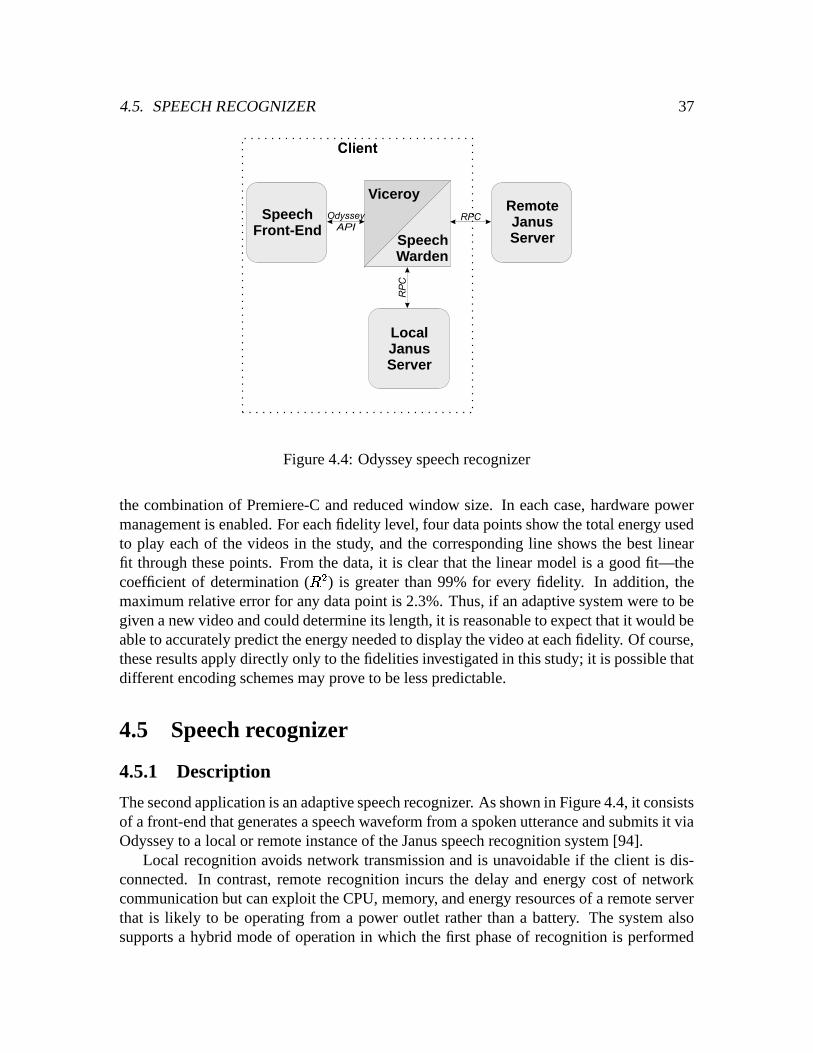
4.5. SPEECH RECOGNIZER 37
LocalJanusServer
RemoteJanusServer
Viceroy
SpeechWarden
SpeechFront-End
Figure 4.4: Odyssey speech recognizer
the combination of Premiere-C and reduced window size. In each case, hardware powermanagement is enabled. For each fidelity level, four data points show the total energy usedto play each of the videos in the study, and the corresponding line shows the best linearfit through these points. From the data, it is clear that the linear model is a good fit—thecoefficient of determination (
���) is greater than 99% for every fidelity. In addition, the
maximum relative error for any data point is 2.3%. Thus, if an adaptive system were to begiven a new video and could determine its length, it is reasonable to expect that it would beable to accurately predict the energy needed to display the video at each fidelity. Of course,these results apply directly only to the fidelities investigated in this study; it is possible thatdifferent encoding schemes may prove to be less predictable.
4.5 Speech recognizer
4.5.1 Description
The second application is an adaptive speech recognizer. As shown in Figure 4.4, it consistsof a front-end that generates a speech waveform from a spoken utterance and submits it viaOdyssey to a local or remote instance of the Janus speech recognition system [94].
Local recognition avoids network transmission and is unavoidable if the client is dis-connected. In contrast, remote recognition incurs the delay and energy cost of networkcommunication but can exploit the CPU, memory, and energy resources of a remote serverthat is likely to be operating from a power outlet rather than a battery. The system alsosupports a hybrid mode of operation in which the first phase of recognition is performed

38 CHAPTER 4. ENERGY-AWARE ADAPTATION
Utterance 1 Utterance 2 Utterance 3 Utterance 40
50
100
150
Ene
rgy
(Jou
les)
Idle
Janus
Odyssey
WaveLAN
Kernel
Base
line
Har
dwar
e-O
nly
Pow
er M
gmt.
Red
uced
Mod
el
Rem
ote
Rem
ote
- Red
uced
Mod
el
Hyb
ridH
ybrid
- R
educ
ed M
odel
This figure shows the energy used to recognize four spoken utterances from one to sevenseconds in length, ordered from right to left above. For each utterance, the first bar showsenergy consumption without hardware power management or fidelity reduction. The sec-ond bar shows the impact of hardware power management alone. The remaining barsshow the additional savings realized by adaptive strategies. The shadings within each bardetail energy usage by activity. Each measurement is the mean of five trials—the errorbars show 90% confidence intervals.
Figure 4.5: Energy impact of fidelity for speech recognition
locally, resulting in a compact intermediate representation that is shipped to the remoteserver for completion of the recognition. In effect, the hybrid mode uses the first phase ofrecognition as a type-specific compression technique that yields a factor of five reductionin data volume with minimal computational overhead.
Fidelity is lowered in this application by using a reduced vocabulary and a less complexacoustic model. This substantially reduces the memory footprint and processing requiredfor recognition, but degrades recognition quality. The system alerts the user of fidelitytransitions using a synthesized voice. The use of low fidelity is most compelling in the caseof local recognition on a resource-poor disconnected client, although it can also be used inhybrid and remote cases.
Although reducing fidelity limits the number of words available, the word-error ratemay not increase. Intuitively, this is because the recognizer makes fewer mistakes whenchoosing from a smaller set of words in the reduced vocabulary. This helps counterbalancethe effects of reducing the sophistication of the acoustic model.

4.5. SPEECH RECOGNIZER 39
0 2 4 6 8
Utterance Length (seconds)
0
20
40
60
80
100E
nerg
y (J
oule
s)
Hardware-Only Power Mgmt.Reduced Model
Figure 4.6: Predicting speech recognition energy use
This figure shows the relationship between system energy use, data fidelity, and utter-ance length. For each level of data fidelity, ten data points show the total energy usedto recognize different utterances (including the ones from Figure 4.5)—the correspond-ing line represents the best linear fit through these points. All measurements were takenwith hardware power management enabled. The (barely noticeable) error bars show 90%confidence intervals for energy use.
4.5.2 Results
Figure 4.5 presents measurements of client energy usage when recognizing four pre-recordedutterances using local, remote, and hybrid strategies at high and low fidelity. The baselinemeasurements correspond to local recognition at high fidelity without hardware power man-agement. Since speech recognition is compute-intensive, almost all the energy in this caseis consumed by Janus.
Hardware power management reduces client energy usage by 33–34%. Such a substan-tial reduction is possible because the display can be turned off and both the network anddisk can be placed in standby mode for the entire duration of an experiment. This assumesthat user interactions occur solely through speech, and that disk accesses can be avoidedbecause the vocabulary, language model and acoustic model fit entirely in physical mem-ory. More complex recognition tasks may trigger disk activity and hence show less benefitfrom hardware power management.
Lowering fidelity by using a reduced speech model results in a 25–46% reduction inenergy consumption relative to using hardware power management alone. This corresponds

40 CHAPTER 4. ENERGY-AWARE ADAPTATION
to a 50–65% reduction relative to the baseline.Remote recognition at full fidelity reduces energy usage by 33–44% relative to using
hardware power management alone. If fidelity is also reduced, the corresponding savings is42–65%. These figures are comparable to the energy savings for remote execution reportedin the literature for other compute-intensive tasks [69, 77]. As the shadings in the fourthand fifth bars of each data set in Figure 4.5 indicate, most of the energy consumed by theclient in remote recognition occurs with the processor idle—much of this is time spentwaiting for a reply from the server. Lowering fidelity speeds recognition at the server, thusshortening this interval and yielding additional energy savings.
Hybrid recognition offers slightly greater energy savings than remote recognition: 47–55% at full fidelity, and 53–70% at low fidelity, both relative to hardware-only power man-agement. Hybrid recognition increases the fraction of energy used by the local Janus code;but this is more than offset by the reduction in network transmission and idle time.
Overall, the net effect of combining hardware power management with hybrid, low-fidelity recognition is a 69–80% reduction in energy usage relative to the baseline. Inpractice, the optimal strategy will depend on resource availability and the user’s tolerancefor low-fidelity recognition. Chapter 7 explores this issue in greater detail.
Figure 4.6 shows speech recognizer energy use as a function of utterance length forfull and reduced fidelity with hardware power management enabled. For both fidelity lev-els, each data point shows the total energy used to recognize one of a set of ten spokenutterances—this set includes the four utterances from Figure 4.5. The corresponding linesshow the best linear fit through these points. The linear model for the baseline fidelityproduces a reasonable fit (93.7% coefficient of determination), while the fit is considerablybetter for the reduced fidelity (99.8%). At the baseline fidelity, the relative error for sixof the ten utterances is less than 10%; at the reduced fidelity, nine utterances have relativeerror less than 10%. While speech recognition is less predictable than video display, theseresults are quite encouraging—simple linear models appear to do a reasonably good job ofpredicting energy use.
4.5.3 Results for Itsy v1.5
I have ported Janus to the Itsy v1.5 pocket computer in order to explore the impact of dif-ferent hardware platforms on energy-aware adaptation. Figure 4.7 presents measurementsof client energy usage for the same four pre-recorded utterances when the speech front-endexecutes on the Itsy v1.5. Since the Itsy does not have a PCMCIA interface, a serial linkwas used as the network transport.
Because the Itsy is an experimental platform, there exists less system support for hard-ware power management than on the ThinkPad laptop. Thus, the results in Figure 4.7 donot reflect the possibility that one could disable the Itsy’s display and serial link when theyare not in use, or that one could reduce the processor clock frequency when CPU load islow.
Contrasting Figures 4.5 and 4.7 shows that the Itsy consumes more energy than the

4.5. SPEECH RECOGNIZER 41
Utterance 1 Utterance 2 Utterance 3 Utterance 40
50
100
150
200
Ene
rgy
(Jou
les)
IdleJanusOdysseyKernel
Base
line
Red
uced
Mod
el
Rem
ote
Rem
ote
- Red
uced
Mod
el
Hyb
ridH
ybrid
- R
educ
ed M
odel
This figure shows the energy used to recognize four spoken utterances from one to sevenseconds in length, ordered from right to left above. The client machine which executesthe recognitions is an Itsy v1.5 pocket computer—the results can be contrasted with Fig-ure 4.5 in which the client machine is an IBM ThinkPad 560 laptop. The first bar showsenergy consumption without fidelity reduction. The remaining bars show the additionalsavings realized by adaptive strategies. The shadings within each bar detail energy usageby activity. Each measurement is the mean of five trials—the (barely noticeable) errorbars show 90% confidence intervals.
Figure 4.7: Energy impact of fidelity for speech recognition on the Itsy v1.5
ThinkPad to perform local speech recognition, but significantly less energy to performhybrid and remote recognition. Although the Itsy is considerably more energy-efficient thanthe ThinkPad, its StrongArm processor is slower. More significantly, the Janus recognizerperforms a large number of floating-point operations, which are emulated in software on theItsy. These factors combine to make local speech recognition prohibitively slow. Althoughaverage power usage is much lower on the Itsy, the total energy needed for local recognitionis higher.
Use of the reduced quality speech model for local recognition provides considerablebenefit on the Itsy, reducing energy usage from 44–49%. During hybrid and remote execu-tion, use of the reduced speech model has little impact. Although the recognition completesmore quickly on the remote server, the Itsy expends very little energy during the additionaltime it must wait for full-quality recognition because its background power usage is verysmall.
Remote recognition uses much less energy on the Itsy. The energy savings from remoteexecution range from 92–94% for full-quality recognition and from 86–90% for reduced-quality recognition. Two factors contribute to this large savings: the lack of floating-pointsupport makes local processing less attractive, and the energy-efficiency of the hardware

42 CHAPTER 4. ENERGY-AWARE ADAPTATION
Execution ThinkPad 560X Itsy v1.5Location Fidelity Normalized Energy Normalized EnergyLocal Full 1.00 1.00Local Reduced 0.64 0.53Remote Full 0.61 0.06Remote Reduced 0.47 0.06Hybrid Full 0.48 0.09Hybrid Reduced 0.36 0.08
This figure compares speech recognition energy usage on the Itsy v1.5 and ThinkPad560X. Each row shows the average energy used to recognize an utterance on the two plat-forms with hardware power management enabled. Each data value is the geometric meanof energy usage, normalized to local energy usage at full fidelity, for the four utterancesshown in Figures 4.5 and 4.7.
Figure 4.8: Comparison of per-platform speech recognition energy use
platform means that very little energy is expended waiting for remote processing requeststo complete.
Hybrid recognition uses more energy than remote recognition on the Itsy, even thoughthe operation completes in less time. The energy impact of performing the first stage ofrecognition locally is greater than the total amount of energy spent waiting for recognitionto complete during fully-remote execution. This has two important implications for remoteexecution. First, it illustrates that tradeoffs between performance and energy conservationexist for common applications. Second, it shows that remote execution decisions must con-sider both the client and its available resources when deciding where to locate functionality.
The speech recognition results give some evidence that the effectiveness of energy-aware adaptation will increase as mobile hardware becomes more energy-efficient. Intu-itively, modifying application behavior can only affect dynamic power usage—backgroundpower usage is fixed by device energy characteristics. Energy-efficient hardware platforms,which have lower background power usage and a greater ratio of maximum dynamic tobackground power usage, will benefit more. The results in Figures 4.5 and 4.7 bear thisout. The maximum energy savings due to fidelity reduction and remote execution is only64–78% on the ThinkPad, but 92–94% on the more energy-efficient Itsy. However, theseresults are biased by the Itsy’s lack of floating-point support, which contributes to someof the energy differential. Figure 4.8 highlights the difference between the two platformsbe showing the energy usage of each fidelity and remote execution location normalized tolocal energy usage at full fidelity.

4.6. MAP VIEWER 43
AnvilMap
Server
Viceroy
MapWarden
Figure 4.9: Odyssey map viewer
4.6 Map viewer
4.6.1 Description
The third application that I measured was an adaptive map viewer named Anvil. As shownin Figure 4.9, Anvil fetches maps from a remote server via Odyssey and displays them onthe client. Fidelity can be lowered in two ways: filtering and cropping. Filtering eliminatesfine detail and less important features (such as secondary roads) from a map. Croppingpreserves detail, but restricts data to a geographic subset of the original map. The clientannotates the map request with the desired amount of filtering and cropping. The serverperforms any requested operations before transmitting the map data to the client.
4.6.2 Results
I measured the energy used by the client to fetch and display maps of four different cities.Viewing a map differs from the two previous applications in that a user typically needsa non-trivial amount of time to absorb the contents of a map after it has been displayed.This period, which I will refer to as think time, should logically be viewed as part of theapplication’s execution since energy is consumed to keep the map visible. In contrast, theuser needs negligible time after the display of the last video frame or the recognition of anutterance to complete use of the video or speech application.
Think time is likely to depend on both the user and the map being displayed. Myapproach to handling this variability was to use an initial value of 5 seconds and thenperform sensitivity analysis for think times of 0, 10 and 20 seconds. For brevity, Figure 4.10only presents detailed results for the 5 second case; for other think times, I present only thesummary information in Figure 4.11.
The baseline bars in Figure 4.10 show that most of the energy is consumed while thekernel executes the idle procedure; a significant portion of this can be attributed to back-ground power usage during the five seconds of think time. The shadings on the bars indicate

44 CHAPTER 4. ENERGY-AWARE ADAPTATION
San Jose Allentown Boston Pittsburgh0
50
100
150
Ene
rgy
(Jou
les)
IdleAnvilX Server OdysseyWaveLANKernel
Base
line
Har
dwar
e-O
nly
Pow
er M
gmt.
Min
or R
oad
Filte
r
Seco
ndar
y R
oad
Filte
r
Cro
pped
Cro
pped
- M
inor
Roa
d Fi
lter
Cro
pped
- Se
cond
ary
Roa
d Fi
lter
This figure shows the energy used to view U.S.G.S. maps of four cities. For each map, thefirst bar shows energy usage without hardware power management or fidelity reduction,with a 5 second think time. The second bar shows the impact of hardware power manage-ment alone. The remaining bars show the additional savings realized by degrading mapfidelity. The shadings within each bar detail energy usage by activity. Each measurementis the mean of ten trials—the error bars are 90% confidence intervals.
Figure 4.10: Energy impact of fidelity for map viewing
that network communication is a second significant drain on energy. The comparativelylarger confidence intervals for this application result from variation in the time required tofetch a map over the wireless network.
Hardware power management reduces energy consumption by about 9–19% relative tothe baseline. Although there is little opportunity for network power management while themap is being fetched, the network can remain in standby mode during think time. Since thedisk is never used, it can always remain in standby mode.
The third and fourth bars of each data set show the effect of fidelity reduction throughtwo levels of filtering. One filter omits minor roads, while the more aggressive filter omitsboth minor and secondary roads. The savings from the minor road filter range from 6–51%relative to hardware-only power management. The corresponding figure for the secondaryroad filter is 23–55%.
The fifth bar of each data set shows the effect of lowering fidelity by cropping a mapto half its original height and width. Energy usage at this fidelity is 14–49% less than withhardware-only power management. In other words, cropping is less effective than filteringfor these particular maps. Combining cropping with filtering results in an energy savings of36–66% relative to hardware-only power management, as shown by the rightmost bars ofeach data set. Relative to the baseline, this is a reduction of 46–70%. There is little savings
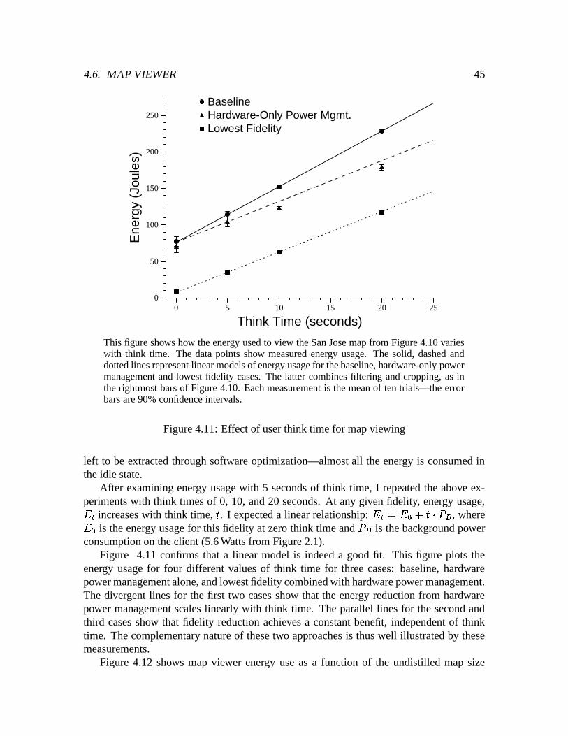
4.6. MAP VIEWER 45
0 5 10 15 20 25
Think Time (seconds)
0
50
100
150
200
250
Ene
rgy
(Jou
les)
BaselineHardware-Only Power Mgmt.Lowest Fidelity
This figure shows how the energy used to view the San Jose map from Figure 4.10 varieswith think time. The data points show measured energy usage. The solid, dashed anddotted lines represent linear models of energy usage for the baseline, hardware-only powermanagement and lowest fidelity cases. The latter combines filtering and cropping, as inthe rightmost bars of Figure 4.10. Each measurement is the mean of ten trials—the errorbars are 90% confidence intervals.
Figure 4.11: Effect of user think time for map viewing
left to be extracted through software optimization—almost all the energy is consumed inthe idle state.
After examining energy usage with 5 seconds of think time, I repeated the above ex-periments with think times of 0, 10, and 20 seconds. At any given fidelity, energy usage,� � increases with think time, � . I expected a linear relationship:
� � � � � � ��� �� , where� � is the energy usage for this fidelity at zero think time and �� is the background powerconsumption on the client (5.6 Watts from Figure 2.1).
Figure 4.11 confirms that a linear model is indeed a good fit. This figure plots theenergy usage for four different values of think time for three cases: baseline, hardwarepower management alone, and lowest fidelity combined with hardware power management.The divergent lines for the first two cases show that the energy reduction from hardwarepower management scales linearly with think time. The parallel lines for the second andthird cases show that fidelity reduction achieves a constant benefit, independent of thinktime. The complementary nature of these two approaches is thus well illustrated by thesemeasurements.
Figure 4.12 shows map viewer energy use as a function of the undistilled map size

46 CHAPTER 4. ENERGY-AWARE ADAPTATION
0 200 400 600 800 1000
Undistilled Map Size (KB)
0
20
40
60
80
Ene
rgy
(Jou
les)
Hardware-Only Power Mgmt.Minor Road FilterCombined
Figure 4.12: Predicting map viewer energy use
This figure shows the relationship between system energy use, data fidelity, and undistilledmap size. For each level of data fidelity, ten data points show the total energy used to viewsix maps (including the ones from Figure 4.10)—the corresponding line represents thebest linear fit through these points. All measurements were taken with hardware powermanagement enabled. The error bars show 90% confidence intervals for energy use.
for three fidelity levels: baseline, minor road filtering, and the combination of minor roadfiltering, secondary road filtering, and cropping. (The remaining fidelity levels are omittedfor clarity). For each fidelity, six data points show the total energy used to fetch and displaydifferent city maps, including the four from Figure 4.10. Since I have already shown thatthe energy cost of user think time is quite predictable, these results assume zero think time,and thereby isolate the variance in the energy cost of fetching and displaying maps.
Visual inspection of the linear fits reveals that energy usage corresponds closely toimage size only in the baseline case. Whereas the baseline has a coefficient of determinationof greater than 99%, the minor road filter and combined fidelities have
� �values of 36%
and 69% respectively. Clearly, the undistilled map size does not remain a good predictorwhen map fidelity is reduced.
When simple models do not yield good predictions, it is possible that additional infor-mation will give more accurate results. In the specific example of the map viewer, the per-centage of features omitted by a given filter may vary widely from map to map. However,if the map server were to store summary information with each map listing the occurrenceof different feature types, one could anticipate the effectiveness of a filter. This would al-low an adaptive system to determine the number of map features that would be fetched at

4.7. WEB BROWSER 47
0 10000 20000 30000 40000 50000
Number of Map Features
0
20
40
60
80
Ene
rgy
(Jou
les)
Hardware-Only Power Mgmt.Minor Road Filter
0 1000 2000 3000 4000 5000
Number of Map Features
0
2
4
6
8
Ene
rgy
(Jou
les)
Combined
Figure 4.13: Predicting map viewer energy use by number of features
This figure shows the relationship between system energy use, data fidelity, and the num-ber of map features. For each level of data fidelity, ten data points show the total energyused to view the six maps from Figure 4.12—the corresponding line represents the bestlinear fit through these points. All measurements were taken with hardware power man-agement enabled. The error bars show 90% confidence intervals for energy use.
various levels of filtering.Figure 4.13 shows the benefit of this additional information. It displays map viewer
energy use as a function of fidelity and the number of features fetched. For clarity, thedata is displayed in two graphs: the graph on the left shows the baseline and minor roadfilter fidelities, while the other graph shows the combined fidelity. Knowledge of the num-ber of features that will be omitted by the minor road filter makes predictions much moreaccurate—the
� �value for the minor-road filter fidelity is now 99%. Unfortunately, al-
though the linear fit for the combined fidelity improves, it is still quite poor with an� �
value of 79%. Although the model can anticipate the effect of filtering, it is still unable tocope with variation in the amount of features removed by cropping.
4.7 Web browser
4.7.1 Description
The fourth application is an adaptive Web browser based on Netscape Navigator, as shownin Figure 4.14. In this application, Odyssey and a distillation server located on either sideof a variable-quality network mediate access to Web servers. Requests from an unmodified

48 CHAPTER 4. ENERGY-AWARE ADAPTATION
DistillationServerNetscape
Viceroy
WebWarden
toWeb
serversPro
xy DistillationServer
Figure 4.14: Odyssey Web browser
Netscape browser are routed to a proxy on the client that interacts with Odyssey. After an-notating the request with the desired level of fidelity, Odyssey forwards it to the distillationserver which transcodes images to lower fidelity using lossy JPEG compression. This issimilar to the strategy described by Fox et al [23], except that control of fidelity is at theclient.
4.7.2 Results
As with the map application, a user needs some time after an image is displayed to absorbits contents. I therefore include energy consumed during user think time as part of theapplication. I use a baseline value of 5 seconds and perform sensitivity analysis for 0, 10,and 20 seconds.
Figure 4.15 presents measurements of the energy used to fetch and display four GIFimages of varying sizes. Hardware power management achieves reductions of 22–26%.The shadings on the first and second bars of each data set indicate that most of this savingsoccurs in the idle state, probably during think time.
The energy benefits of fidelity reduction are disappointing. As Figure 4.15 shows, theenergy used at the lowest fidelity is merely 4–14% lower than with hardware power man-agement alone; relative to baseline, this is a reduction of 29–34%. The maximum benefitof fidelity reduction is severely limited because the relative amount of energy used duringthink time (28 Watts) is much greater than the energy used to fetch and display an image,(2–16 Watts). Thus, even if fidelity reduction could completely eliminate the energy usedto fetch and display an image, energy use would drop only 9–36%.
Although Web fidelity reduction shows little benefit in this study, it may be quite usefulin other environments. For example, a more energy-efficient mobile device would use lessenergy during think time, increasing the possible benefit of fidelity reduction. Similarly, ifa high-speed network were unavailable, the energy benefit of distillation would increase.
The effect of varying think time is shown in Figure 4.16. The linear model introduced

4.7. WEB BROWSER 49
Image 1 Image 2 Image 3 Image 40
20
40
60
Ene
rgy
(Jou
les)
IdleNetscapeCellophaneX Server OdysseyWaveLANKernel
Base
line
Har
dwar
e-O
nly
Pow
er M
gmt.
JPEG
-75
JPEG
-50
JPEG
-25
JPEG
-5
This figure shows the energy used to display four GIF images from 110 B to 175 KB insize, ordered from right to left above. For each image, the first data bar shows energyconsumption at highest fidelity without hardware power management, assuming a thinktime of five seconds. The second bar shows the impact of hardware power managementalone. The remaining bars show energy usage as fidelity is lowered through increasinglyaggressive lossy JPEG compression. The shadings within each bar detail energy usage byactivity. Each measurement is the mean of ten trials—the error bars show 90% confidenceintervals.
Figure 4.15: Energy impact of fidelity for Web browsing
in Section 4.6.2 fits observations well for all three cases: baseline, hardware-only powermanagement, and lowest fidelity. The close spacing of the lines for the two latter casesreflects the small energy savings available through fidelity reduction. The divergence of thelines for the first two cases shows the importance of hardware power management duringthink time.
Figure 4.17 shows Web browser energy use as a function of the undistilled image sizefor three fidelity levels: baseline, JPEG 50, and JPEG 5. For each fidelity, seven data pointsshow the total energy used to fetch and display different images, including the four fromFigure 4.15. As with the map application, these results include no user think-time, therebyisolating the variation in energy used to fetch and display images. For this application,simple linear models yield reasonable predictions: the
� �values for baseline, JPEG 50,
and JPEG 5 are 91%, 93%, and 98% respectively.A related study of Netscape energy usage [64] looks at the relationship between energy
use and image size in more detail. It attributes some of the variation in energy use tothe Netscape application, speculating that the scheduling behavior of Netscape’s user-levelthreading package leads to non-deterministic effects. The study also finds that different

50 CHAPTER 4. ENERGY-AWARE ADAPTATION
0 5 10 15 20 25
Think Time (seconds)
0
50
100
150
200E
nerg
y (J
oule
s)BaselineHardware-Only Power Mgmt.Lowest Fidelity
This figure shows how the energy used to display Image 1 from Figure 4.15 varies withuser think time. The data points on the graph show measured energy usage for user thinktimes of 0, 5, 10, and 20 seconds. The solid, dashed and dotted lines represent linearmodels of energy consumption for the baseline, hardware-only power management, andlowest fidelity cases. Each measurement represents the mean of ten trials—the error barsare 90% confidence intervals.
Figure 4.16: Effect of user think time for Web browsing
images vary slightly in the amount of compression achieved for equivalent levels of JPEGquality.
4.8 Effect of concurrency
How does concurrent execution affect energy usage? One can imagine situations in whichtotal energy usage goes down when two applications execute concurrently rather than se-quentially. For example, once the screen has been turned on for one application, no addi-tional energy is required to keep it on for the second. One can also envision situations inwhich concurrent applications interfere with each other in ways that increase energy usage.For example, if physical memory size is inadequate to accommodate the working sets oftwo applications, their concurrent execution will trigger higher paging activity, possiblyleading to increased energy usage. Clearly, the impact of concurrency can vary dependingon the applications, their interleaving, and the machine on which they run.
What is the effect of lowering fidelity? The measurements reported in Sections 4.4

4.8. EFFECT OF CONCURRENCY 51
0 50 100 150
Unsdistilled Image Size (KB)
0
5
10
15
20
25E
nerg
y (J
oule
s)
Hardware-Only Power Mgmt.JPEG 50JPEG 5
Figure 4.17: Predicting Web browser energy use
This figure shows the relationship between system energy use, data fidelity, and undis-tilled image size. For each level of data fidelity, six data points show the total energy usedto fetch and display different GIF images (including the ones from Figure 4.15)—the cor-responding line represents the best linear fit through these points. All measurements weretaken with hardware power management enabled. The error bars show 90% confidenceintervals for energy use.
to 4.7 indicate that lowering fidelity tends to increase the fraction of energy consumptionattributable to the idle state. Concurrency allows background energy consumption to beamortized across applications. It is therefore possible in some cases for concurrency toenhance the benefit of lowering fidelity.
To confirm this intuition, I compared the energy usage of a composite applicationwhen executing in isolation and when executing concurrently with the video applicationdescribed in Section 4.4. The composite application consists of six iterations of a loop thatinvolves the speech, Web, and map applications described in Sections 4.5 to 4.7. The loopconsists of local recognition of two speech utterances, access of a Web page, access of amap, and five seconds of think time. The composite application models a user searchingfor Web and map information using speech commands, while the video application modelsa background newsfeed. This experiment takes between 80 and 160 seconds.
Figure 4.18 presents the results of the experiments for three cases: baseline, hardware-only power management, and minimal fidelity. In the first two cases, all applications ran atfull fidelity; in the third case, all ran at lowest fidelity. For each data set, the left bar showsenergy usage for the composite application in isolation, while the right bar shows energy
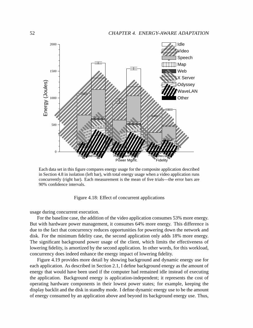
52 CHAPTER 4. ENERGY-AWARE ADAPTATION
Baseline Hardware-Only Power Mgmt.
Lowest Fidelity
0
500
1000
1500
2000E
nerg
y (J
oule
s)Idle
Video
Speech
Map
Web
X Server
Odyssey
WaveLAN
Other
Each data set in this figure compares energy usage for the composite application describedin Section 4.8 in isolation (left bar), with total energy usage when a video application runsconcurrently (right bar). Each measurement is the mean of five trials—the error bars are90% confidence intervals.
Figure 4.18: Effect of concurrent applications
usage during concurrent execution.For the baseline case, the addition of the video application consumes 53% more energy.
But with hardware power management, it consumes 64% more energy. This difference isdue to the fact that concurrency reduces opportunities for powering down the network anddisk. For the minimum fidelity case, the second application only adds 18% more energy.The significant background power usage of the client, which limits the effectiveness oflowering fidelity, is amortized by the second application. In other words, for this workload,concurrency does indeed enhance the energy impact of lowering fidelity.
Figure 4.19 provides more detail by showing background and dynamic energy use foreach application. As described in Section 2.1, I define background energy as the amount ofenergy that would have been used if the computer had remained idle instead of executingthe application. Background energy is application-independent; it represents the cost ofoperating hardware components in their lowest power states; for example, keeping thedisplay backlit and the disk in standby mode. I define dynamic energy use to be the amountof energy consumed by an application above and beyond its background energy use. Thus,
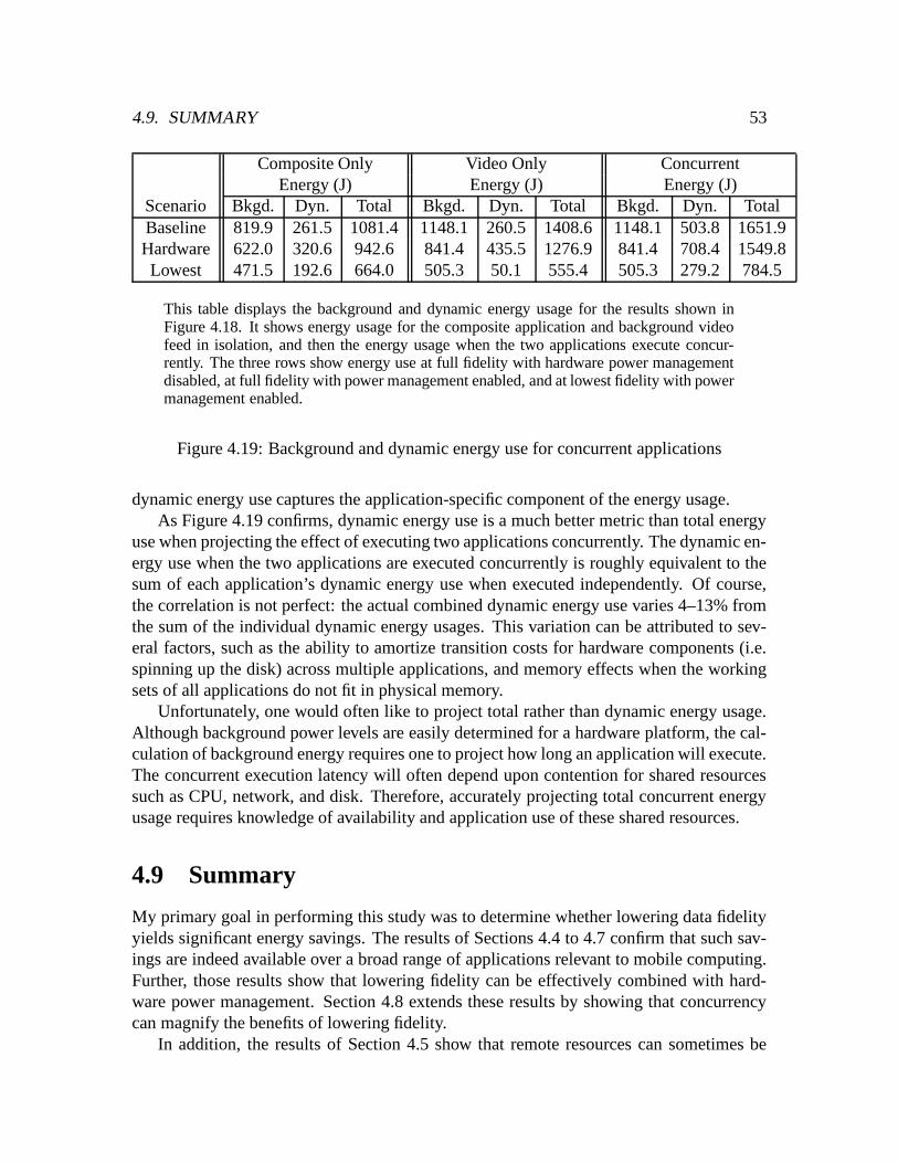
4.9. SUMMARY 53
Composite Only Video Only ConcurrentEnergy (J) Energy (J) Energy (J)
Scenario Bkgd. Dyn. Total Bkgd. Dyn. Total Bkgd. Dyn. TotalBaseline 819.9 261.5 1081.4 1148.1 260.5 1408.6 1148.1 503.8 1651.9Hardware 622.0 320.6 942.6 841.4 435.5 1276.9 841.4 708.4 1549.8
Lowest 471.5 192.6 664.0 505.3 50.1 555.4 505.3 279.2 784.5
This table displays the background and dynamic energy usage for the results shown inFigure 4.18. It shows energy usage for the composite application and background videofeed in isolation, and then the energy usage when the two applications execute concur-rently. The three rows show energy use at full fidelity with hardware power managementdisabled, at full fidelity with power management enabled, and at lowest fidelity with powermanagement enabled.
Figure 4.19: Background and dynamic energy use for concurrent applications
dynamic energy use captures the application-specific component of the energy usage.As Figure 4.19 confirms, dynamic energy use is a much better metric than total energy
use when projecting the effect of executing two applications concurrently. The dynamic en-ergy use when the two applications are executed concurrently is roughly equivalent to thesum of each application’s dynamic energy use when executed independently. Of course,the correlation is not perfect: the actual combined dynamic energy use varies 4–13% fromthe sum of the individual dynamic energy usages. This variation can be attributed to sev-eral factors, such as the ability to amortize transition costs for hardware components (i.e.spinning up the disk) across multiple applications, and memory effects when the workingsets of all applications do not fit in physical memory.
Unfortunately, one would often like to project total rather than dynamic energy usage.Although background power levels are easily determined for a hardware platform, the cal-culation of background energy requires one to project how long an application will execute.The concurrent execution latency will often depend upon contention for shared resourcessuch as CPU, network, and disk. Therefore, accurately projecting total concurrent energyusage requires knowledge of availability and application use of these shared resources.
4.9 Summary
My primary goal in performing this study was to determine whether lowering data fidelityyields significant energy savings. The results of Sections 4.4 to 4.7 confirm that such sav-ings are indeed available over a broad range of applications relevant to mobile computing.Further, those results show that lowering fidelity can be effectively combined with hard-ware power management. Section 4.8 extends these results by showing that concurrencycan magnify the benefits of lowering fidelity.
In addition, the results of Section 4.5 show that remote resources can sometimes be

54 CHAPTER 4. ENERGY-AWARE ADAPTATION
Application Think Baseline Hardware Fidelity CombinedTime (s.) Power Mgmt. Reduction
Video N/A 1.00 0.90–0.91 0.84–0.84 0.65–0.65Speech N/A 1.00 0.66–0.67 0.22–0.36 0.20–0.31
Map 0 1.00 0.80–1.01 0.06–0.13 0.07–0.185 1.00 0.81–0.91 0.38–0.67 0.31–0.54
10 1.00 0.74–0.84 0.53–0.77 0.42–0.5820 1.00 0.76–0.78 0.69–0.89 0.51–0.67
Web 0 1.00 0.85–1.06 0.40–0.75 0.32–0.545 1.00 0.74–0.78 0.88–0.97 0.66–0.71
10 1.00 0.75–0.78 0.93–0.98 0.70–0.7420 1.00 0.74–0.77 0.96–0.99 0.72–0.73
This table summarizes the impact of data fidelity on application energy consumption.Each entry shows the minimum and maximum measured energy consumption on the IBMThinkPad 560X for four data objects. The entries are normalized to baseline measure-ments of full fidelity objects with no power management. This data was extracted fromFigures 4.2, 4.5, 4.10, and 4.15.
Figure 4.20: Summary of the energy impact of fidelity
profitably employed to reduce the energy usage of a mobile client. However, the resultsalso provide a caution: performing computation remotely does not always lead to reducedclient energy use. The hybrid mode of speech recognition uses less energy than the fullyremote mode on the ThinkPad because the energy cost of performing a small amount ofcomputation locally is outweighed by the benefit of decreased energy usage for networktransmission.
The study also reveals that it is often possible to predict the energy impact of fidelityreduction. For the video, speech, and Web applications, simple linear models based onfidelity and input data size provide good fits for application energy use. This means thatan adaptive system could observe an application execute on several data objects at a givenfidelity level, construct a simple model, and use that model to project how much energywill be used when the application operates on new objects at that fidelity level.
The map application shows that achieving accurate energy predictions sometimes re-quires more work. Filtering based upon feature type yields considerable variation in en-ergy reduction. This variation can be accurately modeled, however, if the server stores asummary with each map listing the number of occurrences of each feature type. Croppingintroduces still more variation in energy use. Thus, the map application confirms that therecan often be a tradeoff between complexity and accuracy in predicting energy use.

4.9. SUMMARY 55
At the next level of detail, Figure 4.20 summarizes the results of Sections 4.4 to 4.7.For clarity, the data in each row is normalized to the baseline values.
The key messages of Figure 4.20 are:� There is significant variation in the effectiveness of fidelity reduction across data
objects.
The reduction can span a range as broad as 29% (0.38–0.67 for the map viewer, atthink time 5). The video player is the only application that shows little variationacross data objects. As mentioned above, this variation is often quite predictablewith the use of simple linear models.
� There is considerable variation in the effectiveness of fidelity reduction across appli-cations.
Holding think time constant at 5 seconds and averaging across data objects, the en-ergy usage for the four applications at lowest fidelity is 0.84, 0.28, 0.51 and 0.93relative to their baseline values. The mean is 0.64, corresponding to an average sav-ings of 36%.
� Combining hardware power management with lowered fidelity can sometimes reduceenergy usage below the product of the individual reductions.
This is seen most easily in the case of the video application, where the last columnis 0.65 rather than the expected value of 0.76, obtained by multiplying 0.9 and 0.84.Intuitively, this is because reducing fidelity decreases hardware utilization, therebyincreasing the opportunity for hardware power management.

56 CHAPTER 4. ENERGY-AWARE ADAPTATION

Chapter 5
A proxy approach for closed-sourceenvironments
The previous chapter showed that energy-aware applications can often significantly extendthe battery lifetimes of the laptop computers on which they operate by trading fidelity forreduced energy usage. However, since only multimedia, source-code available applicationsrunning on the Linux operating system were studied, it is not clear whether energy-awareadaptation can help the Windows office applications that users commonly run on laptopcomputers.
Thus, several important questions remain: Can one show significant energy reductionsfor office applications commonly executed on laptop computers? Is it possible to addenergy-awareness without access to application source code? Is this approach valid forapplications executing on source-code unavailable operating systems (i.e. Windows)? Inthis chapter, I will answer these questions by studying the potential benefits of energy-awareadaptation for Microsoft’s popular PowerPoint 2000 application.
5.1 Overview
As with many office applications, PowerPoint enables users to include increasing amountsof rich multimedia content in their documents—for example, charts, graphs, and images.Since these objects tend to be quite large, the processor, network, and disk activity neededto manipulate them accounts for significant energy expenditure. Yet, when editing a pre-sentation, a user may only need to modify and view a small subset of these objects. Thus, itmay be possible to significantly reduce PowerPoint energy consumption by presenting theuser with a distilled version of a presentation: one which contains only the information thatthe user is interested in viewing or editing.
One can use Puppeteer [14], component-based middleware developed by Rice Uni-versity, to perform such distillation. Puppeteer takes advantage of well-defined interfacesexported by applications to change behavior without source code modification. Using Pup-peteer, one can create a distilled version of a presentation which initially omits all multi-
57

58 CHAPTER 5. A PROXY APPROACH FOR CLOSED-SOURCE ENVIRONMENTS
PuppeteerServer Proxy
Client 1
Application
PuppeteerClient Proxy
API
Client 2
Application
PuppeteerClient Proxy
API
Data Sever 1 Data Sever 2 Data Sever 3
Low BW Link Low BW Link
High BW Link High BW LinkHigh BW Link
Tier 4
Tier 3
Tier 2
Tier 1
Figure 5.1: Puppeteer architecture
media content not on the first or master slide. Placeholders are inserted into the documentto represent omitted objects. Later, if the user wishes to edit or view a component, she mayclick on the placeholder, and Puppeteer will load the component and dynamically insert itinto the document. Thus, when the user edits only a subset of a document, the potential forsignificant energy savings exists.
In the remainder of this chapter, I explore the feasibility of adding energy-aware adap-tation to PowerPoint. The next section provides a more detailed description of Puppeteer,and Section 5.3 describes my energy measurement methodology for the Windows plat-form. Section 5.4 measures the impact of energy-aware adaptation while loading, editing,and saving PowerPoint documents, and Section 5.5 summarizes the results.
5.2 Puppeteer
Puppeteer adapts the behavior of component-based applications, such as Microsoft’s Pow-erPoint and Internet Explorer, in response to variation in resource availability in mobileenvironments. While Puppeteer’s design goals are similar to Odyssey’s, its implementationis quite different. It uses the exported APIs of applications and the structured nature of thedocuments they manipulate to change application behavior without source-code modifica-tion. Puppeteer thus acts as a proxy for an application.
Puppeteer currently supports two forms of adaptation: subsetting and versioning. Sub-setting loads only a portion of the elements of a document. Versioning loads differentversions of some elements, for example low-resolution distillations of images.

5.3. MEASUREMENT METHODOLOGY 59
Commercial applications such as Microsoft’s Office suite are ideally suited for Pup-peteer. These applications have well-defined document structures, allowing Puppeteer toparse documents to implement specific policies such as degrading all images of a certainsize. Further, such applications have rich external interfaces that enable Puppeteer to incre-mentally modify loaded documents. For example, Puppeteer can insert additional data orhigher-resolution versions of images using such APIs.
Figure 5.2 shows the Puppeteer architecture. There are four tiers: applications, Pup-peteer client proxies, Puppeteer server proxies, and data servers. Data servers are arbitraryrepositories of data such as Web servers, file servers, or databases. All communication be-tween applications and data servers pass through the Puppeteer client and server proxies.Applications and data servers remain completely unmodified—adaptation is performed byclient and server proxies working in concert.
Puppeteer adjusts to reduced bandwidth availability between a mobile client and dataservers by loading degraded versions of documents. Application-specific policies deter-mine which subset of components should be fetched and which should be degraded. Pup-peteer parses the document to uncover the structure of the data, fetches selected componentsat specific fidelity levels, and updates the application with the newly fetched data.
Once a degraded document version is loaded, the application returns control to the user.Although the application believes that it has loaded the original, full-quality document,Puppeteer maintains a list of degraded and omitted components. While editing or viewinga document, a user may double-click on a degraded component or on a placeholder for anomitted component. Puppeteer then fetches the component at its highest quality and insertsit into the document using the application’s external programming interface.
Puppeteer is currently being modified to allow users to save changes made to degradedversions of documents. Since Puppeteer understands document structure, it can parse themodified version on the client and send to the server only those components which havebeen modified. The server proxy can then merge the modified components into the full-quality version and save the resulting document.
5.3 Measurement methodology
All measurements reported in this chapter were collected in a client-server environmentsimilar to the one used in the previous chapter. PowerPoint executes on the client: an IBM560X laptop, as described in Section 2.2.1. The server is a 400 MHz Pentium II desktopwith 128 MB of memory. Both machines run the Windows NT 4.0 operating system. Themachines communicate using a 2 Mb/s 2.5 GHz Lucent WaveLan network. I added anadditional 32 MB of memory to the client, bringing the total to 96 MB—this was necessaryto run PowerPoint, Puppeteer, and Windows NT without thrashing.
Since PowerPoint source code is unavailable, it made little sense to port PowerScope toWindows to perform these measurements. Instead, I simply measured the amount of totalenergy consumed by the laptop between two points in program execution. The hardwaresetup used for Windows measurements is identical to that used for PowerScope measure-

60 CHAPTER 5. A PROXY APPROACH FOR CLOSED-SOURCE ENVIRONMENTS
Document Full-Quality DistilledPresentation Identifier Size (MB) Size (MB) Ratio
A 24666 15.02 1.67 0.11B 24758 11.42 0.47 0.04C 24890 7.26 0.83 0.11D 26295 3.11 3.11 1.00E 26141 2.23 1.32 0.59F 24773 1.72 0.11 0.07G 25189 1.07 0.36 0.34H 26388 0.87 0.75 0.86I 26140 0.20 0.20 1.00J 25132 0.08 0.08 1.00
Figure 5.2: Sizes of sample presentations
ments. I attached the probes of the HP3458a digital multimeter to the external power inputof the client laptop and removed the battery to eliminate the effects of charging. I alsoconnected the output pin of the client’s parallel port to the multimeter’s external trigger.
I created a dynamic library that allows applications to precisely indicate the start andend of each measurement. An application first calls the start measuring function,which records the current time and toggles the parallel port pin. Once the pin is toggled, themultimeter samples current levels at its maximum rate of 1357.5 times per second. Whenthe event being measured completes, the application calls the stop measuring function,which returns the elapsed time since the start measuring function was called.
To calculate total energy usage, I first derive the number of samples, � , that were takenbefore stop measuringwas called by multiplying the elapsed measurement time by thesample rate. The mean of the first � samples is the average current level. Multiplying thisvalue by the measured voltage for the laptop power supply yields the average power usage.This is multiplied by the elapsed time to calculate total energy usage.
I assume aggressive power management policies. All measurements were taken usinga disk-spindown threshold of 30 seconds (the minimum allowed by Windows NT). Thewireless network uses standard 802.11 power management. However, the display is notdisabled during measurements since PowerPoint is interactive.
5.4 Benefits of PowerPoint adaptation
5.4.1 Loading presentations
I first examined the potential benefit of loading distilled PowerPoint presentations. I mea-sured the energy used to fetch presentations from the remote server over the wireless net-work and render them on the client.
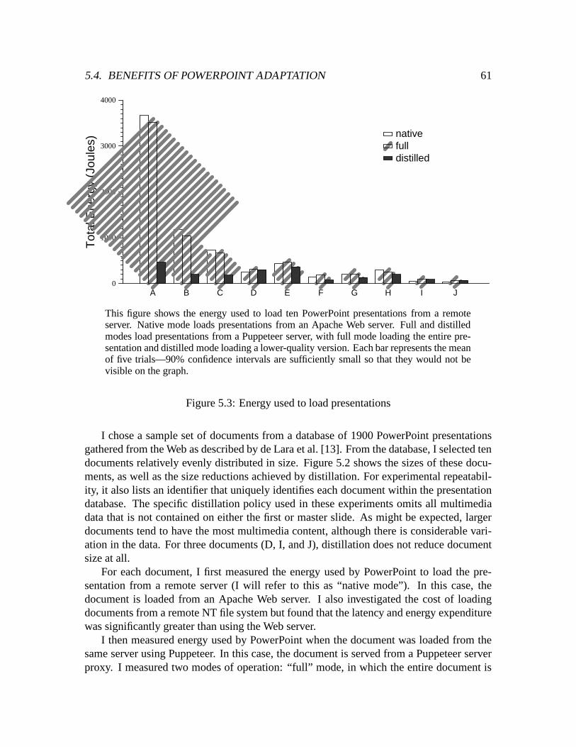
5.4. BENEFITS OF POWERPOINT ADAPTATION 61
A B C D E F G H I J0
1000
2000
3000
4000T
otal
Ene
rgy
(Jou
les)
nativefulldistilled
This figure shows the energy used to load ten PowerPoint presentations from a remoteserver. Native mode loads presentations from an Apache Web server. Full and distilledmodes load presentations from a Puppeteer server, with full mode loading the entire pre-sentation and distilled mode loading a lower-quality version. Each bar represents the meanof five trials—90% confidence intervals are sufficiently small so that they would not bevisible on the graph.
Figure 5.3: Energy used to load presentations
I chose a sample set of documents from a database of 1900 PowerPoint presentationsgathered from the Web as described by de Lara et al. [13]. From the database, I selected tendocuments relatively evenly distributed in size. Figure 5.2 shows the sizes of these docu-ments, as well as the size reductions achieved by distillation. For experimental repeatabil-ity, it also lists an identifier that uniquely identifies each document within the presentationdatabase. The specific distillation policy used in these experiments omits all multimediadata that is not contained on either the first or master slide. As might be expected, largerdocuments tend to have the most multimedia content, although there is considerable vari-ation in the data. For three documents (D, I, and J), distillation does not reduce documentsize at all.
For each document, I first measured the energy used by PowerPoint to load the pre-sentation from a remote server (I will refer to this as “native mode”). In this case, thedocument is loaded from an Apache Web server. I also investigated the cost of loadingdocuments from a remote NT file system but found that the latency and energy expenditurewas significantly greater than using the Web server.
I then measured energy used by PowerPoint when the document was loaded from thesame server using Puppeteer. In this case, the document is served from a Puppeteer serverproxy. I measured two modes of operation: “full” mode, in which the entire document is

62 CHAPTER 5. A PROXY APPROACH FOR CLOSED-SOURCE ENVIRONMENTS
A B C D E F G H I J0
1
2
Nor
mal
ized
Ene
rgy
nativefulldistilled
This figure shows the relative energy used to load ten PowerPoint presentations from aremote server, as described in Figure 5.3. For each data set, results are normalized to theamount of energy used to load the document in native mode.
Figure 5.4: Normalized energy used to load presentations
loaded, and “distilled” mode, in which a reduced-quality version is loaded.Figure 5.3 shows the total energy used to fetch the documents using native, full, and
distilled modes. In Figure 5.4, I show the relative impact for each document by normalizingeach value to the energy used by native mode. The energy savings achieved by distillationvary widely. Loading a distilled version of document A uses only 13% as much energy asnative mode, while distilling document J uses 137% more energy. On average, loading adistilled version of a document uses 60% of the energy used by native mode.
It is interesting to note that full mode can sometimes use less energy to fetch a documentthan native mode. This is because fetching a presentation with Puppeteer tends to useless power than native mode. Thus, even though native mode takes less time to fetch adocument, its total energy usage can sometimes be greater. Without source code, it isimpossible to know for certain why Puppeteer power usage is lower than native mode. Onepossibility is more efficient scheduling of network transmissions.
The results in Figures 5.3 and 5.4 show that while most documents benefit from distilla-tion, some suffer an energy penalty. This indicates that Puppeteer might profit by predictingwhether a document will benefit from distillation. If it predicts that a document will ben-efit, it could distill and fetch it; otherwise, it could forego distillation and fetch the entiredocument.

5.4. BENEFITS OF POWERPOINT ADAPTATION 63
A B C E F G H I J0
200
400
600
Tot
al E
nerg
y (J
oule
s)
full-qualitydistilled
This figure shows the amount of energy needed to page through a presentation. For eachdata set, the left bar shows energy use for a full-quality presentation, and the right barshows energy use for a reduced-quality version of the same presentation. Document D isomitted from this experiment since it contains only a single slide. Each bar represents themean of five trials—the error bars show 90% confidence intervals.
Figure 5.5: Energy used to page through presentations
One possible prediction method is to distill only presentations that have a size greaterthan a fixed threshold, reasoning that small documents are unlikely to contain significantmultimedia content. Analysis of the documents used in this study suggests that a reasonablethreshold is 0.5 MB. A strategy of distilling only presentations larger than 0.5 MB uses 52%of the energy of native mode to load the ten documents.
Another possible prediction method is to distill only those documents with a percentageof multimedia content greater than a threshold value. As shown in Figure 5.2, distillationdoes not reduce the sizes of three documents. If Puppeteer does not distill these documents,it uses only 51% of the energy of native mode to fetch the ten documents.
5.4.2 Editing presentations
I next measured how document distillation affects the energy needed to edit a presentation.While it is somewhat intuitive that loading a smaller, distilled version of a document canrequire less energy, it is less clear that distillation also reduces energy usage while thedocument is being displayed or edited.
Naturally, energy usage depends upon which activities a user performs. While a defini-tive measurement of potential savings requires a detailed analysis of user behavior, one canestimate such savings by looking at the energy used to perform common activities.

64 CHAPTER 5. A PROXY APPROACH FOR CLOSED-SOURCE ENVIRONMENTS
A B C E F G H I J0
200
400
600
Tot
al E
nerg
y (J
oule
s) full-quality - 2nd passfull-quality - 1st passdistilled - 2nd passdistilled - 1st pass
This figure shows the amount of energy needed to page through a presentation a secondtime. The energy needed to page through each presentation the first time is also shown forcomparison. For each data set, the left two bars show energy use for a full-quality presen-tation, and the right two bars show energy use for a reduced-quality version. Document Dis omitted from this experiment since it contains only a single slide. Each bar representsthe mean of five trials—the error bars show 90% confidence intervals.
Figure 5.6: Energy used to re-page through presentations
One very common activity is paging through the slides in a presentation. I createda Visual Basic program to simulate the actions of a user performing this activity. Theprogram loads the first slide, then sends PageDown keystrokes to PowerPoint until allremaining slides have been displayed. After sending each keystroke, the program waits forthe new slide to render, then pauses for a second to simulate user think-time.
I measured the energy used to page through both the full-quality and distilled versionsof each document. Figure 5.5 presents these results for nine of the ten presentations in thesample set—presentation D is omitted because it contains only a single slide. As shown bythe difference in height between each pair of bars in Figure 5.5, distilling a document withlarge amounts of multimedia content can significantly reduce the energy needed to pagethrough the document. Energy savings range from 1% to 30%, with an average of 13%.
After PowerPoint displays a slide, it appears to cache data allowing it to quickly re-render the slide, thereby reducing the energy needed for redisplay. This effect is shown inFigure 5.6, which displays the energy used to page through each document a second time.
For ease of comparison, Figure 5.6 also shows the energy needed to page through eachdocument the first time. Comparing the heights of corresponding bars shows that sub-

5.4. BENEFITS OF POWERPOINT ADAPTATION 65
0
100
200
300
400
Tot
al E
nerg
y (J
oule
s)
0
500
1000
1500
Tot
al E
nerg
y (J
oule
s)
noneauto-correctspell-checkinggrammar-checkingoffice assistant
(a) no interval (b) 100 ms. interval
This figure shows the amount of energy needed to perform background activities duringtext entry. The graph on the left shows energy use when text is entered without pause,and the graph on the right shows energy use with a 100 ms. pause between characters.Each bar shows the cumulative effect of performing background activities, so the leftmostbar in each graph was measured while no background activities were being performed,and the rightmost bar in each graph was measured while all background activities werebeing performed. Each bar represents the mean of five trials—the error bars show 90%confidence intervals.
Figure 5.7: Energy used by background activities during text entry
sequent slide renderings use less energy than the initial renderings. Thus, the benefit ofdistillation is smaller on subsequent traversals of the document: ranging from negligible to20% with an average value of 5%.
5.4.3 Background activities
I next measured the energy used to perform background activities such as auto-correctionand spell-checking. Whenever a user enters text, PowerPoint may perform backgroundprocessing to analyze the input and offer advice and corrections to the user. When batterylevels are critical, such background processing could be disabled to extend battery lifetime.
I measured the effect of auto-correction, spell-checking, style-checking, and providingadvice through the Office Assistant (paperclip). I created a Visual Basic program whichenters a fixed amount of text on a blank slide. The program sends keystrokes to PowerPoint,pausing for a specified amount of time between each keystroke.
Figure 5.7(a) shows the energy used to enter text with no pause between keystrokes;

66 CHAPTER 5. A PROXY APPROACH FOR CLOSED-SOURCE ENVIRONMENTS
Figure 5.7(b) shows energy usage with a 100 ms. pause between keystrokes. I first mea-sured energy usage with no background activities enabled, and then successively enabledauto-correction, spell-checking, style-checking, and the Office Assistant. Thus, the differ-ence between any bar in Figure 5.7 and the bar to its left shows the amount of additionalenergy used to perform a specific background activity. For example, the difference betweenthe first two bars in each graph shows the effect of auto-correction.
Figure 5.7 shows that auto-correction expends negligible energy when entering text—the additional energy can not be distinguished from experimental error. Spell-checking andstyle-checking incur a small additional cost. With no pause between entering characters,employing these options adds a 5.0% energy overhead—with a 100 ms. pause betweencharacters, the overhead is 3.3%.
The Office Assistant incurs a more significant energy penalty. With no pause betweentyping characters, enabling the Assistant leads to a 9.1% increase in energy use. With a100 ms. pause, energy use increases 4.9%. In fact, even when the user is performing noactivity, enabling the Office Assistant still consumes an additional 0.3 Watts, increasingpower usage 4.4% on the measured system. Adaptively disabling the Office Assistant cantherefore lead to a small but significant extension in battery lifetime.
5.4.4 Autosave
Autosave frequency is another potential dimension of energy-aware adaptation. After adocument is modified, PowerPoint periodically saves an AutoRecovery file to disk in orderto preserve edits in the event of a system or application crash. Autosave may be optionallyenabled or disabled—if it is enabled, the frequency of autosave is a configurable parameter.Since autosave is performed as a background activity, it often will have little effect uponperceived application performance. However, the energy cost is not negligible: the diskmust be spun up, and, for large documents, a considerable amount of data must be written.
Since periodic autosaves over the wireless network would be prohibitively slow, I as-sumed that documents are stored on local disk. I created a Visual Basic program to helpquantify the energy impact of autosave. The program loads a PowerPoint document, makesa small modification (adds one slide), and then performs no further activity for twentyminutes. To avoid spurious measurement of initial activity associated with loading andmodifying the presentation, I waited for ten minutes after the modification was made to thedocument before I began measuring power usage.
Figure 5.8 shows power usage for three autosave frequencies. For each presentation, thefirst bar shows power usage when the full-quality version of the document is modified and aone minute autosave frequency is specified. The next bar in each data set shows the effect ofa five minute autosave frequency. The final bar shows the effect of disabling autosave—thisis the maximum power reduction that can be achieved by modifying autosave parameters.
As can be seen by the difference between the first two bars of each data set, changingthe autosave frequency from 1 minute to 5 minutes reduces power usage 5–12%, withan average reduction of 8%. The maximum possible benefit is realized when autosave is

5.5. SUMMARY 67
A B C D E F G H I J0
2
4
6
8
Ave
rage
Pow
er (
Wat
ts)
1 min. autosave5 min. autosaveno autosave
This figure shows how the frequency of PowerPoint autosave affects power usage. Thethree bars in each data set show power use with a 1 minute autosave frequency, with a 5minute autosave frequency, and with autosave disabled. Each bar represents the mean offive trials—the error bars show 90% confidence intervals.
Figure 5.8: Effect of autosave options on application power usage
disabled. As shown by the difference between the first and last bars in each data set, thisreduces power usage 7–18% with an average reduction of 11%. Thus, depending uponthe user’s willingness to hazard data loss in the event of crashes, autosave frequency is apotentially useful dimension of energy-aware adaptation.
5.5 Summary
I began this chapter by asking several questions: Can one show significant energy reduc-tions for office applications commonly executed on laptop computers? Is it possible to addenergy awareness without access to application source code? Is this approach valid forapplications executing on source-code unavailable operating systems (i.e. Windows)?
As the results of Section 5.4 show, the answer to all these questions is “yes”. UsingPuppeteer’s component-based adaptation approach, one can add energy-awareness withoutapplication or operating system source code. Distillation reduces the energy needed toload PowerPoint presentations from a remote server by 49%. Distillation can also lead tosignificant energy savings when editing and saving presentations. Finally, I showed howmodifications such as disabling the Office Assistant and lowering autosave frequency canlead to further energy conservation.

68 CHAPTER 5. A PROXY APPROACH FOR CLOSED-SOURCE ENVIRONMENTS

Chapter 6
System support for energy-awareadaptation
The previous two chapters demonstrated the feasibility of energy-aware adaptation. Theyshowed that applications can modify their behavior to significantly reduce the energy usageof the platforms on which they execute. However, since energy-aware adaptation comes atthe cost of degraded fidelity, applications should only adapt their behavior when neces-sary. This chapter explores how system support can guide applications to make appropriateadaptation decisions.
The next section explores goal-directed adaptation, a feedback technique which esti-mates the importance of reducing energy usage. By measuring energy supply and demand,the operating system is able to determine the correct balance between energy conservationand application fidelity. Section 6.2 then shows how the system can improve the agility ofadaptation decisions by learning from a history of past application energy usage.
6.1 Goal-directed adaptation
Current operating systems provide little support for energy management. Typically, thesystem reports the expected remaining battery lifetime at the current rate of energy usage.In addition, the system usually provides a limited number of device-specific parametersthat modify hardware power management policies.
Users who wish to extend their computer’s battery lifetimes must manually adjust sev-eral parameters such as the screen brightness and disk spin-down timeout to select thecorrect level of energy conservation. In order to set these parameters correctly, they mustdevelop an intuitive notion of how each parameter affects energy use. Further, they mustperiodically observe the estimate for remaining battery lifetime in order to verify that thechosen settings are correct.
Goal-directed adaptation inverts this process by making energy management the re-sponsibility of the operating system. The user specifies only desired battery lifetime. Thesystem assumes responsibility for making the correct tradeoffs between quality and energy
69

70 CHAPTER 6. SYSTEM SUPPORT FOR ENERGY-AWARE ADAPTATION
conservation that ensure that the battery lasts for the specified duration. Rather than adjust-ing power management parameters, the system adjusts application fidelity, using feedbackto determine correct settings. The system also performs the task of monitoring remainingbattery lifetime to ensure that the chosen fidelity settings are correct.
6.1.1 Design considerations
The most important consideration in the design of goal-directed adaptation is ensuring thatthe specified time goal is met whenever feasible. Clearly, users will only trust the system tomanage their battery energy if it proves that it can reliably meet the specified goals. Whena user specifies an infeasible duration, one so large that the available energy is inadequateeven if all applications run at lowest fidelity, the system should detect the problem and alertthe user as soon as possible.
An important secondary goal is providing the best user experience possible. This trans-lates into two requirements: first, applications should offer as high a fidelity as possibleat all times; second, the user should not be jarred by frequent adaptations. Goal-directedadaptation balances these opposing concerns by striving to provide high average fidelitywhile using hysteresis to reduce the frequency of fidelity changes.
When the user specifies a battery lifetime, it is important to recognize that the durationrepresents the amount of work the user wishes to accomplish while on battery power. Adap-tive strategies that extend battery lifetime but accomplish less total work should thereforebe avoided. For example, consider a workload of scientific calculations performed on theItsy v1.5. Reducing processor clock frequency decreases the average power used to per-form a calculation, but increases total energy consumption. Thus, although battery lifetimeis extended, the total number of calculations performed will be decreased. This scenariomakes it clear that fidelity should only be reduced when applications use less total energyper unit of work at the reduced fidelity. All of the fidelity reductions studied in the previoustwo chapters have this property.
6.1.2 Implementation
The Odyssey platform for mobile computing, described in Section 2.3, provides the basisfor implementing goal-directed adaptation. I created a simple user interface that allowsusers to specify goals for battery duration and receive feedback about the feasibility of thespecified goals.
Further, I modified Odyssey to perform three tasks periodically. First, Odyssey deter-mines the residual energy available in the battery. Second, it predicts future energy demand.Third, based on these two pieces of information, it decides if applications should changefidelity and notifies them accordingly.

6.1. GOAL-DIRECTED ADAPTATION 71
Figure 6.1: User interface for goal-directed adaptation
User interface
Often the estimate for needed battery lifetime will be driven by external criteria—for ex-ample, the expected duration of a flight, commute, or meeting. Since the exact durationof such events is often unknown, Odyssey allows the user to respecify the time goal whennecessary. Whenever this happens, Odyssey either adapts to meet the new goal or notifiesthe user that it is infeasible.
Figure 6.1 shows the user interface for goal-directed adaptation. This interface is de-signed to be as simple as possible so as to avoid unnecessary user distraction. The userspecifies the goal for battery duration by adjusting the slider in the middle of the dialog.When conditions change, the user may readjust the slider to specify a new battery goal.As time passes and the battery drains, the slider moves to the left to express the change inexpected remaining battery lifetime. For example, the dialog in Figure 6.1 shows that theexpected remaining battery lifetime is 138 minutes. After one hour, the dialog will show 78minutes of remaining lifetime, assuming that the user does not adjust the battery goal in themeantime. While current operating systems provide similar dialogs, they are output-only;they do not provide users with the ability to change the expected battery lifetime.
The dialog also displays the state of battery management to the user. Figure 6.1 showsthe normal state; the battery lifetime is being managed by Odyssey and the specified goalappears feasible. If Odyssey determines that the goal is infeasible, the interface changesthe dialog title and displays a red background. This warns the user that the battery willexpire sooner than the specified time—the user may then decrease activity or specify ashorter duration. Similarly, when Odyssey determines that the battery will last longer thanthe specified duration even if all applications execute at their highest fidelities, the inter-

72 CHAPTER 6. SYSTEM SUPPORT FOR ENERGY-AWARE ADAPTATION
face changes the dialog title and displays a green background. If the mobile computer isconnected to wall-power, the slider is disabled since goal-directed adaptation is only mean-ingful when the battery is discharging.
Determining residual energy
Odyssey determines residual energy by measuring the amount of charge in the battery.Many modern mobile computers ship with a Smart Battery [79], a gas gauge chip which re-ports detailed information about battery state and power usage. On such platforms, Odysseyperiodically queries the Smart Battery chip to determine remaining battery capacity.
The specific query interface may be machine-dependent. For example, the Itsy v2.2contains a Dallas Semiconductor DS2437 Smart Battery chip [12]. Odyssey queries thebattery through a one-wire bus connected to a general purpose input/output (GPIO) pinof the StrongArm 1100 processor. A Linux device driver for this chip was developed byCompaq Western Research Lab. Once per minute, Odyssey performs an ioctl on thedevice to query remaining capacity.
The Advanced Configuration and Power Interface (ACPI) specification [36] providesa more standard interface to Smart Battery information. The Linux ACPI driver exportsbattery status information through the /proc interface. On the IBM ThinkPad T20 laptop,Odyssey reads the remaining capacity through this interface once every ten seconds.
While the above methods are best for deployed systems, they may not be ideal in lab-oratory settings. Older mobile computers such as the Itsy v1.5 and IBM ThinkPad 560Xlack the necessary hardware support for measuring battery capacity. Additionally, since anactual battery must be used to obtain measurements, it is difficult to control for non-idealbattery behavior. Finally, running large numbers of experiments is difficult because onemust recharge the battery after each trial.
To facilitate evaluation, Odyssey can optionally use a modulated energy supply. At thebeginning of evaluation, the initial value for the modulated supply is specified to Odyssey.As the evaluation proceeds, a digital multimeter samples the actual power usage of themobile computer and transmits the samples to Odyssey. When it receives a new sample,Odyssey assumes constant power consumption between samples and decrements the mod-ulated energy supply by the product of the sampled power usage and the sampling period.When the value of the modulated energy supply reaches zero, Odyssey reports that thebattery has expired.
Predicting future energy demand
To predict energy demand, Odyssey assumes that future behavior will be similar to recently-observed behavior. Odyssey uses smoothed observations of present and past power usageto predict future power use. This approach is in contrast to requiring applications to ex-plicitly declare their future energy usage—an approach that places unnecessary burden onapplications and is unlikely to be accurate.

6.1. GOAL-DIRECTED ADAPTATION 73
Odyssey uses methods similar to those described in the previous section to observepower usage. On the Itsy v2.2, Odyssey queries the Smart Battery to measure current andvoltage levels once per second. It multiplies the two values to calculate power usage. On theThinkPad T20, an artifact of the Linux ACPI driver prevents Odyssey from querying cur-rent and voltage levels. Instead, Odyssey estimates power usage by periodically samplingremaining battery capacity and dividing the difference in capacity by the sample period.When the battery supply is modulated, Odyssey uses the power samples collected by theexternal digital multimeter.
To smooth power estimates, Odyssey uses an exponential weighted average of the form:
new � ����������this sample
� � ������old
�(6.1)
where�
is the gain, a parameter that determines the relative weights of current and pastpower usage. Once future power usage has been estimated, it is multiplied by the timeremaining until the goal to obtain future energy demand.
Odyssey varies�
as energy drains, thus changing the tradeoff between agility and sta-bility. When the goal is distant, Odyssey uses a large
�. This biases adaptation toward
stability by reducing the number of fidelity changes—there is ample time to make adjust-ments later, if necessary. As the goal nears, Odyssey decreases
�so that adaptation is
biased toward agility. Applications now respond more rapidly, since the margin for error issmall.
Currently, Odyssey sets�
so that the half-life of the decay function is approximately10% of the time remaining until the goal. For example, if 30 minutes remain,
�is chosen
so that the present estimate will be weighted equally with more recent samples after ap-proximately 3 minutes have passed. Specifically, if one sample is collected per second, andT is the time remaining to the goal:
� � �� ����� ��� ������� (6.2)
The choice of 10% is based on a sensitivity analysis, discussed in Section 6.1.4.
Triggering adaptation
When predicted demand exceeds residual energy, Odyssey advises applications to reducetheir energy usage. Conversely, when residual energy significantly exceeds predicted de-mand, applications are advised to increase fidelity. In this chapter, fidelity reduction is thesole method of energy conservation—Chapter 7 describes the system support necessary tosupport remote execution as a further dimension of energy conservation.
The amount by which supply must exceed demand to trigger fidelity improvement isindicative of the level of hysteresis in Odyssey’s adaptation strategy. This value is the sumof two empirically-derived components: a variable component, 5% of residual energy, anda constant component, 1% of the initial energy available. The variable component reflects

74 CHAPTER 6. SYSTEM SUPPORT FOR ENERGY-AWARE ADAPTATION
the bias toward stability when energy is plentiful and toward agility when it is scarce;the constant component biases against fidelity improvements when residual energy is low.As a guard against excessive adaptation due to energy transients, Odyssey caps fidelityimprovements at a maximum rate of once every 15 seconds.
To meet the specified goal for battery duration, Odyssey tries to keep power demandwithin the zone of hysteresis. Whenever power demand exceeds those bounds, adaptationis necessary. Odyssey then determines which applications should change fidelity, as wellas the magnitude of change needed for each application. Ideally, the set of fidelity changesshould modify power demand so that it once again enters the zone of hysteresis.
Often, there will be many possible sets of adaptations that yield the needed changein power demand. In these cases, Odyssey must refer to an adaptation policy to decidewhich alternative is best. Although one can implement many different adaptation policies,my initial prototype used a simple one based on user-specified priorities. Each applicationspecifies a list of supported fidelities—lower fidelity levels are assumed to use less energythan higher fidelities. The user assigns static priorities to arbitrate between applications.Odyssey always degrades a lower-priority application before degrading a higher-priorityone—upgrades occur in reverse order. Once the lowest-priority application is degraded toits lowest fidelity level, Odyssey degrades the fidelity of the next lowest-priority applica-tion.
After an application adapts, Odyssey verifies whether the change in power demand issufficient. It resets the estimate of power demand to a value that is precisely in the middle ofthe zone of hysteresis—this represents an optimistic assumption that the change in fidelitywill prove sufficient. As Odyssey takes new power measurements, the estimate of powerdemand will either stay within the zone of hysteresis, indicating that the change in fidelitywas correct, or stray outside the bounds, indicating that additional adaptation is necessary.In the later case, Odyssey will continue to adapt application behavior until it reaches a valuewhere power demand stays within the zone of hysteresis.
In the rest of this chapter, this adaptation policy will be referred to as the incrementalpolicy, because it changes fidelity one step at a time. The incremental strategy is sufficientto evaluate goal-directed adaptation. However, it is clearly inadequate to model many of thepolicies that a user may wish to express. Section 6.2 describes the system support necessaryto support more detailed policies.
6.1.3 Basic validation
Experiment design
To validate goal-directed adaptation, I executed the two energy-aware applications de-scribed in Section 4.8: a composite application involving speech recognition, map viewingand Web access, run concurrently with a background video application. To obtain a con-tinuous workload, the composite application executes every 25 seconds. This has the effectof holding the amount of work (number of recognitions, image views, and map views)constant over time.
6.1. GOAL-DIRECTED ADAPTATION 75
The video application supports four fidelity levels: full-quality, Premiere-B, Premiere-C, and the combination of Premiere-C and reduction of the display window. The speechrecognition component of the composite application supports full and reduced qualityrecognition on the local machine. The map component has four fidelities: full-quality,minor road filtering, secondary road filtering, and the combination of secondary road fil-tering and cropping. The Web component supports the five fidelities shown in Figure 4.15.I prioritized these components so that speech had the lowest priority, and video, map, andWeb had successively higher priority.
Client applications execute on the IBM 560X laptop, and communicate with serversusing a 900 MHz 2 Mb/s Lucent WaveLAN wireless network. To isolate the performanceof goal-directed adaptation, Odyssey uses a modulated energy supply. In addition, Odysseyuses the incremental adaptation policy described in the previous section.
At the beginning of each experiment, I provided Odyssey with an initial energy valueand a time goal. I then executed the applications, allowing them to adapt under Odyssey’sdirection until the time goal was reached or the residual energy dropped to zero. The formeroutcome represents a successful completion of the experiment, while the latter represents afailure. I noted the total number of adaptations of each application during the experiment.I also noted the residual energy at the end of the experiment—a large value suggests thatOdyssey may have been too conservative in its adaptation decisions and that average fidelitycould have been higher.
All experiments used a 12,000 Joule modulated energy supply. This lasts 19:27 minuteswhen applications operate at highest fidelity, and 27:06 minutes at lowest fidelity. The dif-ference between the two values represents a 39.3% extension in battery life. I deliberatelychose a small initial energy value so that I could perform a large number of experiments ina reasonable amount of time. The value of 12,000 Joules is only about 14% of the nominalenergy in the IBM 560X battery. Extrapolating to full nominal energy, the workload wouldrun for 2:18 hours at highest fidelity, and 3:13 hours at lowest fidelity.
Results
Figures 6.2 and 6.3 show detailed results from two typical experiments: one with a 20minute goal, and the other with a 26 minute goal. Figure 6.2 shows how the supply ofenergy and Odyssey’s estimate of future demand change over time during the two exper-iments. In both trials, Odyssey meets the specified goal for battery duration. In addition,once the time goal is reached, residual energy is quite low. The graph also confirms thatestimated demand tracks supply closely. The most visible difference between the two trialsis the slope of the supply and demand lines. After an initial adaptation period of approxi-mately three minutes, Odyssey adjusts power usage in the 26 minute trial in order to extendbattery lifetime.
The four graphs of Figure 6.3 show how the fidelity of each application varies duringthe two experiments. For the 20 minute goal, the high priority Web and map applicationsremain at full fidelity throughout the experiment; the video degrades slightly; and speechruns mostly at low fidelity. For the 26 minute goal, the highest priority Web application runs

76 CHAPTER 6. SYSTEM SUPPORT FOR ENERGY-AWARE ADAPTATION
0 500 1000 1500
Elapsed Time (s)
0
5000
10000
15000E
nerg
y (J
oule
s)
Supply - 26 Minute GoalDemand - 26 Minute GoalSupply - 20 Minute GoalDemand - 20 Minute Goal
This figure shows how Odyssey meets user-specified goals for battery durations of 20 and26 minutes when running the composite and video applications described in Section 4.8.It shows how the modulated supply of energy and the estimated energy demand changeover time.
Figure 6.2: Example of goal-directed adaptation—supply and demand
mostly at the highest fidelity, while the other three applications run mostly at their lowestfidelities. The difference in fidelity levels between the two trials, shown most clearly forthe video application, accounts for the difference in power demand shown in Figure 6.2.For both time goals, applications adapt less frequently at the beginning of the experimentand more frequently as the time goal nears. This shows the effect of the variable gain whichmakes the system stable when the goal is distant and agile when the goal is near.
Figure 6.4 summarizes the results of five trials for each time goal of 20, 22, 24, and 26minutes. These results confirm that Odyssey is doing a good job of energy adaptation. Thedesired goal was met in every trial. In all cases, residual energy was very low: the largestaverage residue, for the 20 minute experiment, is still only 1.2% of the initial energy value.The average number of adaptations by applications is generally low, but there are somecases where it is high. However, the cases that exhibit high number of adaptations are anartifact of the small initial energy value, since the system is designed to exhibit greateragility when energy is scarce.

6.1. GOAL-DIRECTED ADAPTATION 77
0 500 1000 1500
Elapsed Time (s)
Max
Min
Spe
ech
Fid
elity
26 Minute Goal20 Minute Goal
0 500 1000 1500
Elapsed Time (s)
Max
Min
Vid
eo F
idel
ity
0 500 1000 1500
Elapsed Time (s)
Max
MinMap
Fid
elity
0 500 1000 1500
Elapsed Time (s)
Max
MinWeb
Fid
elity
This figure shows how Odyssey meets user-specified goals for battery durations of 20 and26 minutes when running the composite and video applications described in Section 4.8. Itshows changes in application fidelity. The applications are prioritized with speech havingthe lowest priority, and video, map, and Web having successively higher priority.
Figure 6.3: Example of goal-directed adaptation—application fidelity

78 CHAPTER 6. SYSTEM SUPPORT FOR ENERGY-AWARE ADAPTATION
Specified Goal Residue Number of AdaptationsDuration (s) Met Energy (J) Time (s) Speech Video Map Web
1200 100% 145.2 (25.3) 15.3 (1.9) 10.8 (1.6) 11.0 (4.0) 0.4 (0.9) 0.0 (0.0)1320 100% 107.5 (61.5) 12.9 (7.2) 2.8 (0.4) 28.2 (5.2) 1.6 (2.6) 0.0 (0.0)1440 100% 101.2 (22.3) 13.0 (4.5) 5.0 (7.9) 22.6 (9.8) 9.6 (3.8) 1.2 (1.8)1560 100% 60.2 (28.7) 8.7 (5.9) 1.0 (0.0) 6.0 (2.8) 15.4 (4.6) 7.6 (5.9)
This figure shows system behavior when the composite application executes concurrentlywith the video player. Each experiment uses a 12,000 Joule modulated energy supply.Each row shows the result of specifying a different battery-duration goal. The secondcolumn shows the percentage of trials in which the energy supply lasted for at least thespecified duration. The next two columns show the average residual energy at the endof the experiment. The remaining columns show the average number of adaptations per-formed by each application. Each entry represents the mean of five trials with standarddeviations given in parentheses.
Figure 6.4: Summary of goal-directed adaptation
6.1.4 Sensitivity to half-life
The choice of smoothing function is very important in the design of goal-directed adapta-tion. I therefore examined how changing the half-life parameter used to calculate the gain,�
, affects system performance. I used the same experimental setup as in Section 6.1.3. Onthe client, I executed the video application and displayed a half-hour video clip. I useda modulated energy supply of 13,000 Joules and specified a 30 minute time goal so thesupply would last for the entire video.
Figure 6.5 summarizes the results of five trials each for half-life values of 1%, 5%,10%, and 15%. A half-life of 1% is clearly too unstable—the system produces the largestresidue with this value, and the video player adapts excessively. For larger half-life values,the system is more stable. However, with a 15% half-life, the system is insufficiently agile,failing to meet the goal in one of the five trials. I have also encountered similar results inless detailed analysis of other adaptive applications. This led me to the current approach ofusing a 10% half-life to calculate the value of
�.
6.1.5 Validation with longer duration experiments
The short duration (20–30 minutes) of the experiments in Sections 6.1.3 and 6.1.4 allowedme to explore the behavior of Odyssey for many parameter combinations. Having es-tablished the feasibility of goal-directed adaptation, I then ran a small number of longerduration experiments to confirm its benefits in more realistic scenarios.
I used the same experimental setup as in section 6.1.3. I began each experiment with anenergy supply of 90,000 Joules, roughly matching a fully-charged ThinkPad 560X battery.I specified an initial time duration of 2:45 hours, but extended this goal by 30 minutes at

6.1. GOAL-DIRECTED ADAPTATION 79
Half-Life Goal Met Residue (J) Adaptations0.01 100% 204.6 (17.7) 93.6 (3.7)0.05 100% 124.1 (38.0) 33.2 (4.0)0.10 100% 129.2 (21.6) 14.6 (5.4)0.15 80% 97.6 (22.2) 6.8 (2.9)
This figure shows sensitivity to the half-life value used for smoothing. In each experiment,I assume a 13,000 Joule energy supply. The second column shows the percentage of trialsin which the energy supply lasted for at least the specified duration. The next columnshows the residual energy at the end of the experiment. The final column shows thenumber of adaptations performed. Each entry shows the mean of five trials with standarddeviation given in parentheses.
Figure 6.5: Sensitivity to half-life
the end of the first hour. This change reflects the possibility that a user may modify theestimate of how long the battery needs to last. Finally, I used a simple stochastic model toconstruct an irregular workload. During any given minute, each of four applications (video,speech, map, and Web) may independently be active or idle. An active application executesa fixed workload for one minute; for example, the video application shows a one minutevideo, and the map application fetches five maps with five seconds of think time after eachmap display. After each minute, there is a 10% chance of switching states; that is, an activeapplication stays active, and an idle one stays idle, with probability 0.9.
Figure 6.6 presents the results of five trials of this experiment, each generated with adifferent random number seed. In every case, Odyssey succeeded in meeting its time goal.Four of the five trials ended with a residual energy that was less than 1% of the initialsupply. Only in one trial (trial 3) was the residue noticeably higher (2.8%), implying thatOdyssey was too conservative in its adaptation.
In spite of the bursty workload, Figure 6.6 shows fewer adaptations than Figure 6.4,which had a steady workload. This is a consequence of two interactions between the hys-teresis strategy and the longer-duration goal. First, the zone of hysteresis is much larger,since it is proportional to total energy supply. Second, smoothing is more aggressive whenthe goal is distant. Combined, these two factors cause Odyssey to ignore minor fluctuationsin power usage except toward the end of each trial.
6.1.6 Overhead
The power overhead imposed by goal-directed adaptation is the sum of the overhead ofmeasuring power usage and the overhead of using these measurements to predict energy de-mand. The measurement overhead is quite low. Most Smart Battery solutions can providepower measurements at the frequency Odyssey requires using less than 10 mW. [12, 88].Additionally, if a mobile computer already includes a Smart Battery (as with the IBM T20laptop and Itsy v2.2), Odyssey imposes minimal additional measurement overhead.

80 CHAPTER 6. SYSTEM SUPPORT FOR ENERGY-AWARE ADAPTATION
Trial Goal Residual Number of AdaptationsMet Energy (J) Speech Video Map Web
1 Yes 345 1 5 5 12 Yes 381 1 10 7 113 Yes 2486 8 13 5 04 Yes 554 2 10 6 85 Yes 464 5 6 14 0
This figure shows system behavior for bursty workloads. In each trial, I assume an energysupply of 90,000 Joules. After one hour, the initial goal of 2.75 hours is extended by ahalf hour. Each row shows the result of a trial using a different randomly-generated work-load. The second column shows whether the energy supply lasted for at least the specifiedduration. The next column shows the residual energy at the end of the experiment. Theremaining columns show the number of adaptations performed by each application.
Figure 6.6: Longer duration goal-directed adaptation
I have measured Odyssey’s prediction overhead and found it to be only 4 mW. There-fore, the total power overhead imposed by goal-directed adaptation is less than 14 mW.—only 0.25% of the background power consumption of the IBM 560X.
6.2 Use of application resource history
The previous section showed that goal-directed adaptation can be successfully implementedwithout needing to anticipate how changes in application fidelity affect power usage. Theincremental adaptation policy allows Odyssey to eventually converge on the fidelity levelthat correctly balances energy use and application quality. Yet, when Odyssey can antic-ipate the relationship between fidelity and power use, it can be more agile in adapting tochanges in power demand. In addition, anticipating this relationship allows applicationsspecify a more natural range of fidelities and adaptation policies.
This section describes how Odyssey obtains these benefits by maintaining a historyof application energy usage. The work on which this section reports was done jointlywith Dushyanth Narayanan [64]. As applications execute, Odyssey monitors and logs thefidelities at which they operate and their corresponding energy consumption. From the data,Odyssey learns functions which relate fidelity and energy usage. From these functions,Odyssey predicts how power usage changes with fidelity.
Next, I examine in more detail the benefits of using application resource history topredict future behavior. Section 6.2.2 describes how Odyssey measures and logs energyusage. Section 6.2.3 describes how Odyssey uses the data to learn functions which predictapplication energy use; Sections 6.2.4 and 6.2.5 show how the learned functions are usedto improve adaptation decisions. Section 6.2.6 then demonstrates how Odyssey uses thehistory of application energy usage to increase the effectiveness of goal-directed adaptation.

6.2. USE OF APPLICATION RESOURCE HISTORY 81
6.2.1 Benefits of application resource history
If Odyssey cannot determine the relationship between fidelity and energy use, it will not beable to anticipate the magnitude of change in power usage that will result when applicationschange fidelity. Thus, when Odyssey desires to increase or decrease power use, it mustadapt application fidelity one discrete step at a time. Further, after each adaptation, it mustpause to assess how much power usage has changed.
This means that application fidelities must be carefully chosen, since the number offidelities affects the agility of the system. If a large number of fidelities are specified,Odyssey is sluggish to react to changes in power supply and demand. Before arriving at thecorrect fidelity, it must transition through many intermediate fidelity levels, pausing at eachone to assess the impact of the adaptation on power usage. Potentially, Odyssey may evenmiss the specified goal for battery duration if it is not sufficiently agile in adapting when adecrease in power usage is needed. At the other extreme, if only a small number of fidelitiesare specified, the system may oscillate between two widely-separated fidelity levels becauseno intermediate value is available, leading to an excessive number of adaptations.
However, when Odyssey can predict how fidelity changes will affect energy usage,it can calculate the exact change in application fidelity that will yield a desired changein power usage. It can then adjust fidelity directly to the new value without traversingthrough intermediate values. With this approach, the number of fidelity levels specified byan application will not directly impact system agility.
Use of energy history also lets applications support a more natural range of fidelities andadaptation policies. Applications can specify continuous dimensions of fidelity, whereas ifOdyssey uses the incremental policy, only a single, discrete dimension of fidelity can bespecified (since Odyssey can only adapt in discrete steps). Applications can also specifyadaptation policies which directly relate fidelity and energy use. For example, applicationsmay wish to specify policies such as “Choose the best fidelity that uses no more than x%of the energy of the highest fidelity” or “Degrade fidelity if the decrease in energy useis greater than the corresponding decrease in fidelity”. Odyssey can only evaluate suchpolicies if it is able to predict the amount of energy that will be used at different fidelities.
6.2.2 Recording application resource history
Odyssey’s fundamental unit of history is an operation: a discrete unit of work performed byan application at one of possibly many fidelities. For example, each application describedin Chapter 4 performs one basic operation: the video player displays videos, the speechrecognizer recognizes utterances, the map viewer displays maps, and the Web browserdisplays images.
Odyssey and applications collaborate to generate a history of application energy use.Applications initially describe the operations that they plan to execute, including possiblefidelities and input parameters, variables that affect the complexity of the operation. Theythen signal Odyssey when the execution of each operation begins and ends. During execu-tion, Odyssey measures energy usage. Later, when the operation completes, Odyssey logs

82 CHAPTER 6. SYSTEM SUPPORT FOR ENERGY-AWARE ADAPTATION
register_fidelity (char* conf_file,int* optype_id);
begin_fidelity_op (const char* dataname,int optype_id,int num_params,fid_param_val_t* params,int num_fidelities,fid_param_val_t* fidelities,int* opidp);
int end_fidelity_op (int optype_id,int opid,int failed);
Figure 6.7: Odyssey multi-fidelity API
its energy usage, fidelity, and input parameters.Figure 6.7 shows the relevant portion of Odyssey’s multi-fidelity API, through which
applications provide the information Odyssey needs to log resource usage. Initially, appli-cations call register fidelity() to describe the types of operations that they planto execute. For each operation type, the application specifies the name of a configurationfile. Odyssey returns a unique identifier for the operation type—the application uses theidentifier in future calls.
Figure 6.8 shows the configuration file for the Web browser described in Section 4.7.The first line specifies the names of the application and operation type. The next line namesa file to which resource history will be logged. The third line describes the single inputparameter to the operation, the number of bytes in the uncompressed image. The fourthline describes the single fidelity, which is the degree of JPEG compression to be employed.The configuration file specifies that this dimension of fidelity is continuous and ranges invalue between 5 and 100. Odyssey also allows applications to specify discrete parametersor fidelities which can take on one of several enumerated values. The remainder of theconfiguration file is not relevant to history logging, and will be described in Section 6.2.4.
Before executing an operation, applications call begin fidelity op(), which hastwo purposes. It asks Odyssey which fidelity should be used for the operation. It alsosignals Odyssey to begin measuring resource usage for the operation. The applicationspecifies the name of the data object being manipulated (i.e. the title of a video, the nameof a Web image, etc.), as well as the type of operation to be performed. The applicationalso specifies the specific values of input parameters to the operation. For example, the Webbrowser obtains the number of bytes of the image to be fetched from the HTML headersand passes the information to Odyssey. Odyssey returns the fidelity at which the operation

6.2. USE OF APPLICATION RESOURCE HISTORY 83
description web:fetchimagelogfile /usr/odyssey/etc/web.fetchimage.logparam imagesize ordered 0-10000000fidelity compression ordered 5-100mode normalhintfile /usr/odyssey/lib/web_fetchimage_hints.soutility web_fetchimage_utility
Figure 6.8: Sample configuration file for a Web browser
should be performed, as well as a unique handle by which the application can refer to theoperation.
After an operation completes, the application calls end fidelity op. This causesOdyssey to write an entry in the appropriate log file. Each entry includes resource usageinformation, such as the time and energy to execute the operation. Each entry also containsthe value of each input parameter and the fidelity at which the operation was performed.
Odyssey measures energy usage as described in Section 6.1.2. If the hardware platformsupports ACPI, Odyssey queries the amount of energy remaining in the battery at the startand end of each operation. The difference between the two values is the total energy usedby the operation. If battery level information is not available, Odyssey samples power us-age during operation execution, and calculates energy usage by multiplying average powerusage by execution time. For example, when executing on the Itsy v2.2, Odyssey reads cur-rent levels from the DS2437 Smart Battery chip six times per second. These measurementsare multiplied by the last voltage reading and the duration of the sample period to calculatethe total energy use during the measurement period. Odyssey accumulates the energy mea-surements taken during operation execution, and logs the sum as the total energy usage ofthe operation.
Both methods for measuring operation energy use are inadequate if more than one oper-ation executes simultaneously. With concurrent operations, it is unclear what percentage ofthe total energy expenditure should be attributed to each operation. One possible methodfor apportioning energy usage would be to allocate energy usage according to the per-centage of CPU, disk, network, and other resources used by the operation. However, thismethod requires detailed resource accounting, as well as per-platform calibration of theenergy costs of activities such as network transmissions and disk accesses. I have there-fore chosen the simpler approach of excluding from the history log any operation whichoverlaps with another simultaneous operation. This sacrifices some data, but increases theaccuracy of the logged values.

84 CHAPTER 6. SYSTEM SUPPORT FOR ENERGY-AWARE ADAPTATION
6.2.3 Learning from application resource history
From the history of application resource usage, Odyssey learns functions which relate in-put parameters and fidelity to energy usage. As the study of application energy usage inChapter 4 shows, simple linear models provide a good fit for many applications. Odysseysupports this common case by providing library routines which generate linear models ofenergy use from log data.
Odyssey reads the previously logged data whenever an application registers a new op-eration type. From the data, Odyssey generate a linear model of energy usage. If theoperation type has a continuous dimension of fidelity or a continuous input parameter, amodel is generated using linear regression. If more than one continuous dimension exists,multiple variable linear regression is used. When the operation type has one or more dis-crete dimensions, Odyssey generates a different linear model for each possible combinationof enumerated values. For example, the speech application discussed in Section 4.5.1 hasone discrete dimension of fidelity: it can use either a full-sized or reduced vocabulary forrecognition. For this application, Odyssey develops two separate linear models, one foreach possible fidelity.
Later, Odyssey queries the model to determine how much energy an operation is likelyto use if it is performed with different combinations of fidelity and input parameters. Some-times, there will not be enough data to return a specific prediction, for example, if the op-eration has not yet been performed for one of the possible values of an enumerated type.In this case, the predictor returns a more generic prediction for energy use, one that isgenerated from a model that ignores the enumerated type.
In theory, for some applications, the relationship between energy use and fidelity may bequite complex. Odyssey supports such applications by allowing them to supply application-specific functions for predicting energy usage. In practice, I have found that the defaultlinear models suffice for all applications that I have studied, including those described inChapter 4.
6.2.4 Using application resource history to evaluate utility
Odyssey uses the history of application resource usage to determine the best fidelity atwhich to execute operations. For each operation, Odyssey chooses the one that maximizesthe value of an application-specific utility function specified in the configuration file. Forexample, in Figure 6.8, the last two lines specify that the Web application’s utility functionis web fetchimage utility() in the library web fetchimage hints.so.
A utility function takes as input specific values for each input parameter and fidelitydimension, and returns a numerical result that represents the desirability of executing theoperation with those values. When an application calls begin fidelity op, Odysseysearches the space of possible fidelities to select the fidelity which maximizes the value ofthe utility function. Input parameters are fixed to those specified by the application in thebegin fidelity op call; fidelity varies as the search progresses.

6.2. USE OF APPLICATION RESOURCE HISTORY 85
extern fidelity desired_fidelity;
int utility (fidelity f)�
if (f == desired_fidelity)�
return (1);�else
�
return (0);��
Figure 6.9: Utility function for the incremental policy
The Odyssey multi-fidelity solver, further described in [64], exhaustively searches dis-crete dimensions of fidelity and uses gradient-descent heuristics to search continuous di-mensions. Thus, it is not guaranteed to find an optimal solution in all cases. The solveriteratively calls an operation’s utility function, and selects the fidelity at which the utilityfunction returns the highest value.
Energy-aware applications specify utility functions which balance fidelity and energyuse. Goal-directed adaptation determines the current importance of energy conservation;utility functions express a specific policy for adapting to that importance.
Section 6.1.3 described the simple incremental adaptation policy: each applicationspecifies a single, discrete dimension of fidelity, and Odyssey increases or decreases fi-delity by one step whenever supply and demand diverge. One can trivially express thispolicy as a utility function, shown in Figure 6.9. Odyssey represents the desired fidelity foran application with a global parameter, ��������� � �������� �� ��� . The utility function returns 1 ifthe fidelity passed into the function is equal to ��������� � �������� �� ��� , and 0 otherwise. Thus,the function will be maximized only when the input fidelity is equivalent to the desiredfidelity.
However, this simple policy has a clear drawback: the assumption that all operationsshould be performed at the same fidelity, irrespective of the values of the input parameters.Figure 6.10 illustrates why this assumption is incorrect. Each line shows how Web browserenergy use at a specific fidelity varies with an input parameter, the uncompressed imagesize. The highest fidelity, shown by the solid line, occurs when the image is shown withoutdistillation. The remaining two lines show energy usage when the image is distilled toJPEG quality levels of 99 and 95. Data points show specific measured energy values for twoimage sizes: 3.5 MB, and 720 KB. For large images, the highest fidelity uses more energysince it transmits the most data over the wireless network. However, for small images, thelower fidelities use more energy because image distillation introduces a significant latencywhich results in the client waiting longer for the image to arrive.

86 CHAPTER 6. SYSTEM SUPPORT FOR ENERGY-AWARE ADAPTATION
0 1000 2000 3000 4000
Undistilled Image Size (KB)
0
100
200
300
400E
nerg
y (J
oule
s)Undistilled JPEG-99JPEG-95
This figure shows how Web browser energy usage varies with fidelity and the size of theuncompressed image. The three lines show how energy usage changes with image size forthree different fidelities; the data points represent measured energy usage for two specificimage sizes.
Figure 6.10: Web energy use as a function of fidelity and image size
Now consider the following example scenario. Originally, the application can show allimages at the highest fidelity and still meet the specified goal for battery lifetime. However,when the user extends the goal, the system must adapt to reduce energy usage by a smallamount (5%). If the system lowers fidelity to JPEG-99, it saves energy if a large (3.5 MB)image is displayed, but uses more energy if a small (720 KB) image is displayed. The sys-tem could possibly select the JPEG-95 fidelity, which saves energy for both sizes. However,this needlessly degrades large images—JPEG-99 is sufficient to reduce energy usage 5%.Also, for images smaller than 500 KB, JPEG-95 uses more energy than the highest fidelity.
The above scenario shows that it is often impossible to select a fidelity which producesthe needed change in energy usage across all possible input parameters. Thus, it is infeasi-ble for goal-directed adaptation to adjust application fidelity directly; a fidelity choice thatis correct for one set of input parameters may not be correct for another. To surmount thisproblem, Odyssey introduces a layer of indirection in the form of a global feedback pa-rameter, � , that represents how critical energy conservation is at the current moment. Thevalue of the parameter ranges from 0, when energy usage is unimportant, to 1, when it isof utmost importance. When Odyssey wishes to adjust application behavior, it changes thevalue of � , rather than adjust application fidelity directly.

6.2. USE OF APPLICATION RESOURCE HISTORY 87
extern double c;extern fidelity min_fidelity, max_fidelity;
int utility (fidelity f)�
if ((energy(f) / energy(max_fidelity)) <= (1-c))�
return (goodness(f));�else if (f == min_fidelity)
�
return (0.01); /* Small value */�else
�
return (0);��
Figure 6.11: Utility function for history-based policy
The utility functions of energy-aware applications use the value of � to decide the cor-rect tradeoff between fidelity and energy use. For example, one could ask each applicationto select the best possible fidelity which uses only
��� ���
as much energy as the highestfidelity. When the value of � is 0.1, each application would reduce its energy usage byat least 10%. Given a specific fidelity value, the utility function for this policy, shown inFigure 6.11, uses the history of application energy usage to predict the amount of energyneeded to perform the operation at the specified fidelity. It compares that value to the en-ergy needed to perform the same operation at the highest possible fidelity. If the ratio ofthe two energy values is higher than desired, i.e. greater than
��� ���, the function returns
zero, signifying that the input fidelity should not be chosen. When the ratio between thetwo values is less than
��� ���, Odyssey returns a numerical value corresponding to the
goodness of the fidelity. Thus, the utility function selects the best fidelity supported bythe application that meets the goal for energy reduction. In the event that no fidelity pro-vides the desired energy reduction, the utility function returns a small positive value for thefidelity that conserves the most energy, ensuring that it will be selected.
Alternative policies are also possible. For example, one could select the fidelity whichyields the greatest “bang-for-the-buck”, i.e. the one which yields the greatest decrease inenergy usage for the smallest decrease in fidelity. In all such policies, the history of appli-cation energy usage plays a vital role. Odyssey can correctly evaluate such utility functionsonly by anticipating how much energy an operation will consume at various fidelity levels.
An important consideration is whether Odyssey should represent the importance ofenergy conservation with a single, global feedback parameter or with one parameter foreach currently running application. Multiple feedback parameters would allow Odyssey tooptimize energy usage across applications. For example, one application may be able toconserve a large amount of energy with a small decrease in fidelity, and thereby avoid the

88 CHAPTER 6. SYSTEM SUPPORT FOR ENERGY-AWARE ADAPTATION
need for other applications to adapt. However, the optimization problem is very complex—Odyssey would need to search the space of all possible fidelities for all applications si-multaneously, while possibly considering other important factors such as user-specifiedapplication priorities.
I have therefore chosen to simplify the problem by using only a single, global feed-back parameter. This allows Odyssey to implement “fair” adaptation policies, for example,asking each application to decrease energy usage by a fixed percentage. User-specified pri-orities can be easily incorporated. For instance, one could use an approach similar to lotteryscheduling [95] to prioritize applications; if one application has twice as many tickets asanother, it would be asked to reduce its energy usage only half as much as the other.
6.2.5 Using application resource history to improve agility
Odyssey uses the history of application energy usage to improve the agility of goal-directedadaptation. During normal operation, predicted energy demand remains close to the avail-able supply; it stays in a zone of hysteresis with a value no greater than the energy sup-ply and no lower than the 95% of the current supply minus 1% of the initial energy sup-ply. When demand strays significantly from supply, Odyssey changes the value of theglobal feedback parameter, � . When Odyssey increases � , application behavior is biasedtowards energy conservation; when Odyssey decreases � , applications execute operationswith higher fidelity.
Without application energy history, it is difficult for Odyssey to determine the amountby which it should adjust � . The incremental approach, as described in Section 6.1.2,adjusts � by a small, fixed amount, then pause to assess if the resulting change in powerdemand is sufficient. If many small steps are needed, the system is slow to react to changesin power supply and demand.
However, when application history is available, Odyssey adapts more agilely. Odysseyfirst calculates the current power demand as described in Section 6.1.2. It then calculatesthe ideal power demand, one that falls in the middle of the zone of hysteresis. If
�is the
current energy supply, � the time remaining to the goal, and� �
the initial energy supply, theideal power demand, � � �� �� is:
� � �� �� � � � � � ������ � � �� � � � ��� � � � (6.3)
In principle, Odyssey simply predicts the ideal value of � , �� � �� ��
, that will produce afuture power drain of � � �� �� . Then, Odyssey sets the value of � directly to �
� � �� ��without
needing to traverse through intermediate values.Unfortunately, Odyssey cannot calculate �
� � �� ��directly. Utility functions return the de-
sirability of each fidelity given a specific value of � . There exists no inverse function whichreveals what value of � would yield a specified fidelity (and, hence, a specified power drain).Because utility functions are application-specified, they are, in effect, black boxes, makingthe construction of the inverse function prohibitively difficult. Additionally, when diverse

6.2. USE OF APPLICATION RESOURCE HISTORY 89
Background Power
t = 0t = -5t = -10t = -15
Time
Power
2 W
4 W
6 W
Op 4
Op 3
Op 1Op 2
This figure shows a hypothetical example of how Odyssey calculates the impact of thechoice of the feedback parameter, � , on power demand. Odyssey calculates the dynamicenergy usage of each operation performed in the recent past—this is represented by theboxes labeled “Op 1” through “Op 4”. Odyssey adds each operation’s dynamic powerusage to the background power usage of the hardware platform to generate a waveformthat predicts how power usage would have varied over time, given a specific value of �
(0.1 in this case).
Figure 6.12: Example of operation history replay for � = 0.1
operations are being performed by multiple applications, the utility functions for each op-eration may return different fidelities depending upon operation type and the value of theinput parameters.
Odyssey takes a more indirect route to calculate �� � �� ��
. It assumes that the recent pastpredicts the future, and asks the following question: What (ideal) value of c would haveyielded the ideal power usage in the past?.
Odyssey maintains an in-memory list of operations that have executed recently. Eachlist item records the variables previously used to determine operation fidelity, includinginput parameters and resource availability. Odyssey can therefore revisit past fidelity de-cisions, and calculate what its decision would have been if conditions had been different.Specifically, Odyssey can determine what fidelity it would have chosen for various valuesof � .

90 CHAPTER 6. SYSTEM SUPPORT FOR ENERGY-AWARE ADAPTATION
Background Power
t = 0t = -5t = -10t = -15
Time
Power
2 W
4 W
6 W
Op 3Op 1
Op 2
Op 4
This figure continues the hypothetical example of how Odyssey calculates the impact ofthe choice of the feedback parameter, � , on power demand. It shows predicted powerdemand for � = 0.2.
Figure 6.13: Example of operation history replay for � = 0.2
To calculate �� � �� ��
, Odyssey replays the operation log to determine how power demandvaries with � . For a given value of � , Odyssey first determines the fidelity at which eachpast operation would have executed. It then predicts the amount of dynamic energy eachoperation would have used. It uses the history of application energy usage to predict thetotal energy that would have been used to perform an operation. From this value, it calcu-lates dynamic energy usage by subtracting out background power usage, i.e. the productof the background power usage of the mobile computer and the execution latency of theoperation.
Odyssey then constructs a hypothetical waveform that captures its prediction of howthe mobile computer’s power usage would have changed over time for the specified valueof � . The waveform reflects the background power usage of the machine and the predicteddynamic energy usage of each operation performed in the past. Finally, Odyssey calculatespower demand by applying the exponential smoothing function shown in Equation 6.1 tothe waveform.
Figure 6.12 shows a hypothetical example that helps illustrate this process. Here,

6.2. USE OF APPLICATION RESOURCE HISTORY 91
Odyssey predicts power demand when c is equal to 0.1. There are four recently exe-cuted operations—consider operation 1 which executed for 4 time units starting at time-15. Odyssey first determines the fidelity at which operation 1 would have executed if �
were equal to 0.1. It then predicts the operation’s dynamic energy usage by consulting thehistory of application energy usage. In this example, Odyssey predicts that operation 1’sdynamic energy usage would be 12 Watts. It also performs similar calculations for the otherthree operations.
Odyssey then generates the waveform that represents predicted power usage over time.Total power usage at any given time is the sum of the background power usage of thehardware platform and the dynamic power usage of each currently executing operation.As shown in Figure 6.12, Odyssey makes the simplifying assumption that operation powerusage is constant over the life of an operation. In this figure, the total power usage waveformis given by the area under all shaded regions.
Odyssey determines what its estimate for power demand would have been if it had seenpower usage equivalent to the generated waveform. It starts at the beginning of the wave-form and calculates the exponential weighted average of power demand using Equation 6.1.In the given example, Odyssey would predict power demand to be about 3.81 Watts. Thisentire calculation can be thought of as solving a function,
� ���
which maps � to powerdemand.
Figure 6.13 shows the same calculation for a different value of � . When � increases to0.2, Odyssey selects lower fidelity levels for each operation. Consequently, the dynamicenergy usage of each operation is lower than in Figure 6.12. For � � �� � , Odyssey wouldpredict power demand to be about 3.18 Watts.
Odyssey first determines the impact of the current value of � :� �
��� ����� � � ��. It then per-
forms a binary search on � to determine �� � �� ��
; i.e. the value of �� � �� ��
such that� �
�� � �� �� � �
� ���� ����� � � �
�is closest to � � �� �� � � ����� � � � . When this value is found, Odyssey sets the new
value of � to be �� � �� ��
, and changes its current estimate of power usage by� �
�� � �� �� � �
� ���� ����� � � �
�.
In the example given by Figures 6.12 and 6.13, if ��� ����� � � � were 0.1, and Odysseyneeded to reduce power demand by 0.63 Watts, then �
� � �� ��would be 0.2 since
� � �� � � �� � �� � � � ���� Watts.Why does Odyssey use each operation’s dynamic power usage to calculate �
� � �� ��? As
shown in Section 4.8, when multiple applications execute concurrently, dynamic powerusage is a much better metric than total power usage for calculating each application’simpact. Thus, dynamic power usage is a better metric for assessing the impact of changing
� when operations execute concurrently. Figures 6.12 and 6.13 illustrate this possibilitysince the execution of operations 3 and 4 overlap.
The use of dynamic power as a metric makes one important simplification: it assumesthat changing fidelity will not affect when subsequent operations are started. For exam-ple, when using a speech recognizer, a user may pause a fixed amount of time betweenutterances. Lowering fidelity may speed recognition and allow the user to start the nextrecognition sooner. Predicting such effects is difficult because the system must anticipate

92 CHAPTER 6. SYSTEM SUPPORT FOR ENERGY-AWARE ADAPTATION
0 20 40 60 80 100
Web Fidelity
0
50
100
150
Ene
rgy
(Jou
les)
This figure shows how energy varies with fidelity level for the Web browser described inSection 4.7. Fidelities 5–99 show the energy used by the client to wait for a remote serverto distill a 720 KB GIF image to the corresponding JPEG quality level, fetch the imagefrom the server, and display it to the user. Fidelity 100 shows the energy used to fetchand display the image without distillation. Each data point shows the average amount ofenergy used; the error bars are 90% confidence intervals.
Figure 6.14: Energy use as a function of fidelity for the Web browser
the usage pattern of the application; I have therefore chosen to ignore these effects in cal-culating �
� � �� ��. Errors due to this simplification will eventually be detected by the feedback
mechanism of goal-directed adaptation. However, they may cause Odyssey to convergemore slowly on the correct value of � .
6.2.6 Validation
Experimental design
I validated the benefit of application resource history by executing two experimental sce-narios: one which uses the incremental adaptation policy described in Section 6.1.2, andone which uses the history-based policy described in Section 6.2.5. Each scenario modelsthe actions of a user browsing digital photographs from an album stored on a remote server.The user loads 5 images per minute—each image is approximately 720 KB in size.
Odyssey and the Web browser execute on the client: an IBM 560X laptop computer.The images are stored on a local server running the Odyssey distiller and an Apache Web

6.2. USE OF APPLICATION RESOURCE HISTORY 93
0 2000 4000 6000 8000 10000
Time (seconds)
0
20000
40000
60000
80000
100000E
nerg
y (J
oule
s)
SupplyIdeal
This figure shows how the supply of energy changes over time when Odyssey uses theincremental adaptation policy. The solid line shows the actual change in energy usage—the dashed line shows the hypothetical change that would be achieved by an ideal adaptivepolicy.
Figure 6.15: Change in energy supply for the incremental policy
server. The two machines are connected by a 900 MHz 2 Mb/s Lucent WaveLAN wirelessnetwork.
The Web application performs one type of operation: fetching an image from the server.JPEG quality is the sole dimension of fidelity for the operation. It is specified as a discretedimension ranging from 5 to 100. There are 96 discrete fidelities, making this a challeng-ing scenario for the incremental adaptation policy. Fidelity 100 corresponds to loading anundistilled image—the remaining fidelities correspond to distilling the image to the equiva-lent JPEG quality level before fetching it from the remote server. The image size is the soleinput parameter for the operation. However, image size is not relevant in these experimentssince all images are of roughly the same size.
I first obtained a detailed history of energy usage by performing 4000 image loads froma set of similarly-sized digital photographs. Figure 6.14 summarizes the logged data foroperation energy usage. At any given fidelity, energy use is fairly predictable, with higherquality levels tending to use more energy than lower ones. There is a discontinuity in the

94 CHAPTER 6. SYSTEM SUPPORT FOR ENERGY-AWARE ADAPTATION
0 2000 4000 6000 8000 10000
Time (seconds)
0
20
40
60
80
100
Fid
elity
Web FidelityIdeal
This figure shows how Web fidelity changes over time when Odyssey uses the incrementaladaptation policy. The solid line shows actual Web fidelity levels—the dashed line showsthe hypothetical fidelity levels that would be selected by an ideal adaptive policy.
Figure 6.16: Change in fidelity for the incremental policy
data: fidelity 100 uses less energy than fidelities 97–99. The reduction in data transmittedover the network is small at fidelities 97–99. The energy savings due to reduced networkusage is less than the additional energy the client expends waiting for the server to distillthe image. At this image size, fidelities 97–99 are clearly inferior to fidelity 100 becausethey expend more energy to fetch a lower-quality image. Therefore, a correct adaptationpolicy should not employ these fidelities.
After gathering resource history data, I executed five trials for each adaptation policy.I used a modulated energy supply and specified an initial energy value of 90,000 Joules,roughly equivalent to the amount of energy in the ThinkPad’s battery. I specified an initialtime goal of 2.5 hours. After 1 hour of execution, I modified the time goal by specifyingthat the battery should last an additional 15 minutes.

6.2. USE OF APPLICATION RESOURCE HISTORY 95
0 2000 4000 6000 8000 10000
Time (seconds)
0
20000
40000
60000
80000
100000E
nerg
y (J
oule
s)
SupplyIdeal
This figure shows how the supply of energy changes over time when Odyssey uses thehistory-based adaptation policy. The solid line shows the actual change in energy usage—the dashed line shows the hypothetical change that would be achieved by an ideal adaptivepolicy.
Figure 6.17: Change in energy supply for the history-based policy
Results
Figures 6.15 and 6.16 show results from one typical trial using the incremental adaptationpolicy. The solid line in Figure 6.15 shows how energy supply changes over time; thedashed line shows the ideal rate of drain that would be achieved by a hypothetical, perfectadaptive strategy. In the trial, the rate of drain tracks the ideal fairly closely for the firsthour, although energy is used at a slightly higher rate during this time period. Once theuser requests an additional 15 minutes of battery life, the two lines diverge more noticeably.Odyssey uses too much energy after the adjustment and is never able to recover fully. Theenergy supply expires almost 3 minutes too early.
Figure 6.16 gives more insight into why Odyssey misses the time goal. The solid lineshows the fidelity levels used by the Web application throughout the trial. The dashed lineshows the fidelity levels that would be used by the ideal adaptive policy. The ideal policyuses knowledge of future activity to select the highest constant fidelity which will meet the

96 CHAPTER 6. SYSTEM SUPPORT FOR ENERGY-AWARE ADAPTATION
0 2000 4000 6000 8000 10000
Time (seconds)
0
20
40
60
80
100
Fid
elity
Web FidelityIdeal
This figure shows how Web fidelity changes over time when Odyssey uses the history-based adaptation policy. The solid line shows actual Web fidelity levels—the dashed lineshows the hypothetical fidelity levels that would be selected by an ideal adaptive policy.
Figure 6.18: Change in fidelity for the history-based policy
specified goal for battery life. The ideal policy does not have future knowledge of changesin the specified goal—hence, there is a change in fidelity at the 1 hour mark.
After the user changes the specified time goal at 3600 seconds, Web fidelity decreasesexponentially. Initially, changes in fidelity are relatively infrequent because the goal isdistant. As the goal nears, Odyssey is more agile and fidelity changes are more frequent.Web fidelity remains higher than ideal for a significant portion of time: from 3600 to 6435seconds, causing the laptop to expend too much energy during this period. Even thoughOdyssey tries to compensate by lowering fidelity for the remainder of the trial, it is unableto conserve enough energy to meet the specified goal for battery duration.
It is also interesting to note that the incremental adaptive policy chooses Web fidelities97–99 during the time period lasting from 1845 to 3113 seconds. Without applicationhistory, it cannot know that these fidelities are clearly inferior to fidelity 100. This accountsfor the slight overconsumption of energy during the first hour of the trial.
Figures 6.17 and 6.18 show results from one typical trial using the history-based adap-tation policy. As can be seen in Figure 6.17, the rate of drain of the energy supply tracks

6.2. USE OF APPLICATION RESOURCE HISTORY 97
Adaptation Goal Expiration Number ofPolicy Met? Time (s) Adaptations
Incremental 0% +79.7 (9.7) 56.8 (11.2)History-Based 100% -146.6 (11.2) 7.8 (1.3)
This figure compares the effectiveness of adaptation with and without the use of applica-tion resource history. The first row shows results without application history; the secondrow shows results when history is used to guide adaptation. For each scenario, the secondcolumn shows the percentage of trials that met the specified time goal. The third columnshows the average expiration time for the energy supply, relative to the specified timegoal. The final column lists the average number of adaptations per trial. Five trials wereperformed for each scenario—standard deviations are given in parentheses.
Figure 6.19: Summary of the effectiveness of application resource history
the ideal quite closely. Odyssey maintains a slight surplus throughout the trial and meetsthe goal for battery duration. Once the goal is reached, the amount of residual energyremaining is small: approximately 1.0% of the initial energy supply.
Figure 6.18 shows the corresponding changes in application fidelity. For the first hour,Odyssey chooses fidelities that are close to ideal. It also avoids the clearly inferior fidelitiesfrom 97 to 99. When the user respecifies the goal, Odyssey immediately decreases fidelity.The initially chosen fidelity is slightly less than ideal, reflecting Odyssey’s conservativebias. However, Odyssey soon detects the discrepancy and readjusts the fidelity to be closerto ideal. In contrast to the previous scenario, Odyssey is much more agile in convergingupon an acceptable fidelity level. Using application history, Odyssey requires only twoadaptations to reach a good fidelity choice—without application history, Odyssey is toosluggish, and fails to reach an acceptable fidelity.
Figure 6.19 summarizes the results of the five trials. Use of application resource historyprovides a clear benefit. All five trials that used resource history met the time goal—theenergy supply lasted an average of 79.7 seconds longer than the specified duration. Whenthe incremental policy was used, the energy supply expired too early in all trials—on av-erage, the supply expired 146.6 seconds before the time goal. Further, the average numberof adaptations is much smaller with the history-based policy because Odyssey convergesmuch more quickly upon acceptable fidelity levels.
The use of application history incurs some additional overhead, especially when Odysseydetermines a new value for the feedback parameter � . During the five trials, Odyssey spentan average of 0.83 seconds to calculate a new value for � . However, since this calculationoccurs relatively infrequently, an average of 8 times per 3.25 hour trial, the effect on overallperformance is minimal.
It is worth noting that this scenario represents a difficult challenge for the incrementalpolicy because the Web application has a large number of fidelities and the difference inenergy usage between two consecutive fidelity levels is usually very small. One can poten-tially avoid the problems encountered in this scenario if one carefully chooses the number

98 CHAPTER 6. SYSTEM SUPPORT FOR ENERGY-AWARE ADAPTATION
of potential fidelity levels for the application. For example, in the experiment reported inSection 6.1.3, I specified only five potential fidelities for the Web application. In addition,none of the five fidelities were clearly inferior to any other fidelity. Thus, with carefultuning and a bit of black magic, it is possible to make the incremental policy approachthe performance of the history-based policy. Conversely, one of the main benefits of thehistory-based policy is that it is self-tuning—it requires no special adjustments in order toyield acceptable results.
6.3 Summary
In this chapter, I have shown how goal-directed adaptation allows Odyssey to effectivelymanage battery energy as a resource. The user provides hints that specify how long amobile computer needs to operate on battery power, and Odyssey meets the specified goalsby adjusting the fidelity of energy-aware applications.
Odyssey monitors energy supply and demand to determine the current importance ofenergy conservation. It predicts future energy demand from measurements of past us-age. When there is substantial mismatch between predicted demand and available en-ergy, Odyssey notifies applications to adapt. Using this approach, I have demonstratedthat Odyssey can extend battery life to meet user-specified goals that vary by up to 30%.
I have also shown how the use of application resource history improves the effectivenessof goal-directed adaptation. When energy-aware applications execute, Odyssey monitorsand logs their energy use. From the logged data, it learns functions which relate fidelity andinput parameters to energy usage, allowing it to predict future application energy consump-tion. With these predictions, Odyssey can support a wider range of adaptation policies,including those which directly relate energy and fidelity. Further, Odyssey reacts moreagilely to changes in power demand, adjusting application fidelity to appropriate levelswithout the need to traverse through intermediate values.

Chapter 7
Remote execution
Whenever there exists the possibility of trading some dimension of quality or performancefor reduced energy usage, energy-aware adaptation is possible. While application fidelityis an important dimension of energy-aware adaptation, it is by no means the only one.
Remote execution is another such dimension. If applications execute part of their func-tionality on remote infrastructure, they may reduce their use of local hardware resourcesand conserve energy. However, energy reduction can come at a price. Remote executioncan lead to decreased performance, primarily due to the need to transfer data between localand remote machines. In such cases, energy-aware adaptation is necessary to balance thecompeting concerns of energy use and performance.
This chapter describes Spectra, a remote execution system designed for battery-poweredmobile clients used in pervasive computing environments. Spectra enables applications tocombine the mobility of small devices with the greater resources of large, wall-poweredcompute servers. Spectra provides applications with a mechanism for executing remoteoperations, while ensuring data consistency between local and remote machines. It mon-itors both application resource usage and the availability of resources in the environmentin order to provide dynamic advice to applications about how and where they can mostprofitably execute functionality. Spectra is tightly integrated with Odyssey and leveragesOdyssey’s support for energy-aware adaptation. Its advice lets applications dynamicallybalance the competing goals of performance, energy use, and application fidelity.
The next two sections discuss Spectra’s target environment and design considerations.Section 7.3 describes Spectra’s implementation, and Section 7.4 presents an evaluation ofthe system.
7.1 Target environment
Spectra is targeted at pervasive computing environments—such environments are saturatedwith computing and communication capability, yet gracefully integrated with human users.The need for graceful integration leads to smaller, less obtrusive computing devices. Sincepeople are naturally mobile, these devices are often battery powered, and their size limits
99

100 CHAPTER 7. REMOTE EXECUTION
the amount of energy that can be stored. In addition, device size constrains the availabilityof other resources such as compute power and storage capacity. Remote execution usingwireless networks to access compute servers fills a natural role in pervasive computing,allowing applications to combine the mobility of small devices with the greater resourcesof static, wall-powered compute servers
Future support for mobile applications will vary widely with location. Some well-conditioned environments may provide plentiful wireless bandwidth and powerful computeservers. Other locations may be resource-impoverished, with poor connectivity and littleinfrastructure support. Pervasive applications must therefore adapt to a changing environ-ment. When little infrastructure exists, they must execute most functionality on the mobileclient. However, when the environment is well-conditioned, they should discover and usethe resources offered.
A broad range of resource-hungry applications such as speech recognition, natural lan-guage translation, and augmented reality will be important in pervasive computing envi-ronments. These applications may be executed on a wide range of mobile hardware, frompowerful laptops to wristwatch-sized devices. While customizing these applications foreach platform is possible, it would be more desirable to create a single implementation thatadjusts its behavior to match the platform.
Variation in the environment and in client capability makes it quite difficult for de-velopers to statically determine which components of an application should be executedremotely. Instead, location decisions should be made dynamically when applications exe-cute.
Spectra simplifies the task of developing applications for pervasive computing. Appli-cations statically specify which code components might possibly profit from remote execu-tion. When applications execute, Spectra continually monitors resource supply and demandto advise them how and where they should execute the specified components. Spectra’s ad-vice lets applications adapt to changes in resource availability without requiring them toexplicitly specify their resource requirements. Instead, Spectra monitors application be-havior, models their resource usage, and predicts future resource needs.
Spectra targets applications which perform remote operations of one second or morein duration. Examples of such applications include speech recognition, rendering for aug-mented reality, and document preparation. Location decisions for these types of applica-tions significantly impact performance and energy consumption. Thus, it is often beneficialto invest some effort to ensure that the correct decision is made. Applications which per-form remote operations of shorter duration, for example, tens of milliseconds, will not ben-efit from Spectra since system overhead will negate the performance and energy benefitsachieved by making correct location decisions.
7.2 Design considerations
Pervasive computing introduces several unique challenges for remote execution. In thissection, I discuss these challenges and how they are addressed in the design of Spectra.

7.2. DESIGN CONSIDERATIONS 101
7.2.1 Competing goals for functionality placement
In pervasive computing environments, a remote execution system must reconcile multiple,possibly contradictory goals. Performance remains important, but is no longer the soleconsideration. It is also vital to conserve energy so as to prolong battery lifetime. Qualitymust also be considered explicitly, since a resource-poor mobile device may only be able toprovide a low fidelity version of a data object or computation, while a stationary machinemay be able to generate a better version. These goals will often conflict—for example,executing a code component on a remote server might offer reduced client energy usage atthe cost of increased execution time.
Spectra explicitly considers these competing goals when advising applications whereto place functionality. For each alternative placement, it predicts application performance,energy use, and quality. It then balances competing goals when selecting from the alter-natives using the system support for energy-aware adaptation discussed in the previouschapter. I have therefore chosen to tightly integrate Spectra and Odyssey. One can viewSpectra as an extension to Odyssey that supports remote execution as a second dimensionof energy-aware adaptation.
Together, Spectra and Odyssey advise applications how and where they should exe-cute functionality. By simultaneously considering both execution location and applicationfidelity, they can make better choices than if they considered location and fidelity indepen-dently.
7.2.2 Variation in resource availability
Pervasive computing is characterized by tremendous variation in resource availability. Net-work characteristics and remote infrastructure available for hosting computation vary withlocation. File cache state and CPU load on local and remote machines significantly im-pact application performance. Application energy consumption varies depending upon thespecific platform on which the application executes. Thus, variation in any resource cansignificantly change the optimal placement of functionality. A remote execution systemmust continually monitor resource availability and adapt to changes in the environment.
Spectra includes a set of resource monitors that measure local and remote resourceavailability. Each monitor measures a single resource or set of related resources—for ex-ample, the network monitor reports available bandwidth and latency to remote servers. Themonitors are implemented in a modular framework, which enables developers to easily addmeasurement capability for new resources.
7.2.3 Self-tuning operation
To predict the time and energy needed to execute a code component, the remote execu-tion system must match resource availability with the resource demands of the component.For example, the time needed to transfer data over a network can be roughly predicted by

102 CHAPTER 7. REMOTE EXECUTION
dividing the amount of data that the application will transfer by the available network band-width. Thus, a remote execution system must have a model of application resource demandin order to make correct placement decisions.
One possible approach would be to require applications to explicitly specify their re-source requirements. However, this seems infeasible for most applications. Many resourcesare important in pervasive computing, and an application would have to specify models foreach. Also, models for some resources are platform specific—application energy usage,for instance, depends upon hardware characteristics. The burden of specifying such mod-els seems too high; few developers would be willing to invest the necessary effort.
Spectra takes an alternate, self-tuning, approach. It observes applications execute, mea-sures their resource usage, and generates models of resource consumption. It then uses themodels to predict future demand.
7.2.4 Modification to application source code
Systems such as Coign [32] provide remote execution services without source code modifi-cation by exploiting externally visible object interfaces. This approach is attractive becauseit supports closed-source applications and requires little development effort. However, alittle application-specific knowledge can go a long way.
Spectra asks developers to specify possible methods of partitioning applications. Oftenthere will be only a few useful partitions. While developers will often have an intuitivenotion of which partitions are useful, it may prove difficult to automatically extract suchpartitions from source code. First, the best partitions may not occur along object bound-aries. Second, since the number of potential partitions is exponential with the number ofobjects, selecting partitions for large applications may be computationally intractable. Fi-nally, it will be impossible to support legacy applications which do not provide externallyvisible object interfaces.
Application-specific knowledge can also be used to improve models of resource de-mand. Often resource usage will depend upon a few application-specific parameters—forexample, the amount of CPU cycles required to translate a sentence from Spanish to En-glish often depends upon the length of the sentence to be translated. Spectra provides aninterface that allows applications to specify the operations they perform and the importantparameters that affect operation complexity. Spectra models consider the effect of theseparameters, leading to more accurate predictions.
I have tried to situate Spectra in a sweet spot of the design space. In exchange for aminimal amount of source code modification, Spectra provides significantly better adviceabout how and where to execute functionality than could be provided by a system thatrequires no application modification.
The benefits provided by Spectra increase with the amount of effort that developersinvest. For applications without an interactive interface such as a compiler or Latex, Spec-tra provides considerable benefit without source code modification. Spectra can executesuch applications entirely on a remote server or on the client. Spectra learns application

7.2. DESIGN CONSIDERATIONS 103
resource requirements and chooses the best location for execution. With some source codemodification, Spectra provides additional benefits. If one identifies specific code compo-nents that may benefit from remote execution and inserts Spectra calls in the application,Spectra chooses the best partitioning of functionality between local and remote machines.If one then adds the ability to execute these components at multiple fidelities, Spectra alsochooses the best fidelity for each component. Finally, one can specify input parametersfor each operation and application-specific prediction algorithms that improve the accu-racy of Spectra’s decisions. Thus, developers can choose the right amount of source codemodification for each application.
7.2.5 Granularity of remote execution
A key issue in the design of a remote execution system is the granularity of code that can beexecuted remotely. Fine-grained remote execution yields increased flexibility since it cre-ates more opportunities to locate functionality on remote servers. However, coarse-grainedremote execution may lead to better performance since it often reduces the volume of net-work transmission and amortizes the overhead of deciding where to locate functionalityover a larger unit of execution.
Since Spectra is designed to make intelligent placement decisions that balance com-peting goals and adjust to changes in resource availability, its decision overhead is non-negligible. Therefore, Spectra targets applications that perform relatively coarse-grainedoperations—currently one second or more in duration. Examples of such applications in-clude speech recognition and language translation. Applications that perform shorter re-mote operations, i.e. a few milliseconds in duration, will not benefit from Spectra sincesystem overhead will negate the performance and energy benefits achieved by making cor-rect location decisions.
7.2.6 Support for remote file access
Many of Spectra’s target applications access a large amount of file data. For remote execu-tion to yield correct results, file operations performed on remote servers must produce thesame results that would be produced if the operation were performed on the client. Sys-tems such as Butler [67] solve this problem by using a distributed file system that presentsa consistent file system image across all machines on which functionality may be executed.
Unfortunately, file consistency comes at significant cost in pervasive computing envi-ronments. Network connections to file servers often exhibit high latency, low bandwidth, orintermittent connectivity. When an application modifies files, it will block for long periodsof time waiting for data to be reintegrated to file servers.
This performance consideration led me to adopt the Coda file system [40]. Coda pro-vides strong consistency when network conditions are good. Under low bandwidth con-ditions, Coda buffers file modifications on the client to improve performance. Bufferedmodifications are reintegrated to file servers in the background. Until a modification is
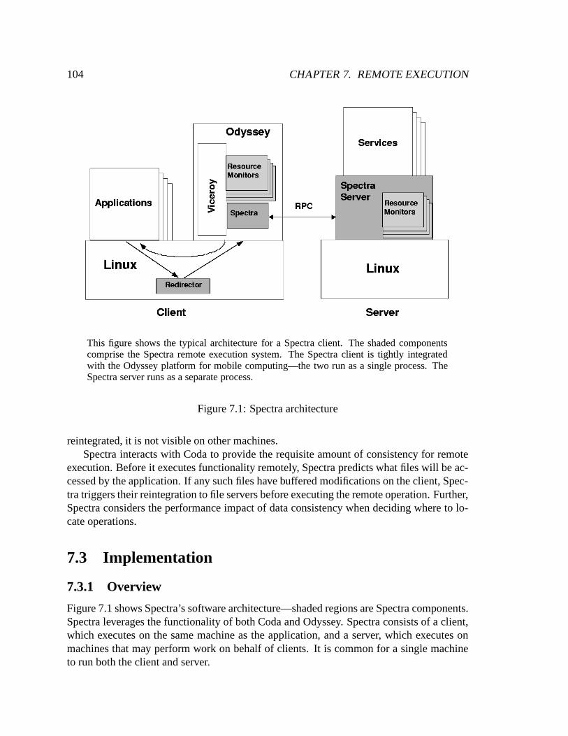
104 CHAPTER 7. REMOTE EXECUTION
This figure shows the typical architecture for a Spectra client. The shaded componentscomprise the Spectra remote execution system. The Spectra client is tightly integratedwith the Odyssey platform for mobile computing—the two run as a single process. TheSpectra server runs as a separate process.
Figure 7.1: Spectra architecture
reintegrated, it is not visible on other machines.Spectra interacts with Coda to provide the requisite amount of consistency for remote
execution. Before it executes functionality remotely, Spectra predicts what files will be ac-cessed by the application. If any such files have buffered modifications on the client, Spec-tra triggers their reintegration to file servers before executing the remote operation. Further,Spectra considers the performance impact of data consistency when deciding where to lo-cate operations.
7.3 Implementation
7.3.1 Overview
Figure 7.1 shows Spectra’s software architecture—shaded regions are Spectra components.Spectra leverages the functionality of both Coda and Odyssey. Spectra consists of a client,which executes on the same machine as the application, and a server, which executes onmachines that may perform work on behalf of clients. It is common for a single machineto run both the client and server.

7.3. IMPLEMENTATION 105
The tight integration between Spectra and Odyssey is reflected in Figure 7.1. The Spec-tra client and Odyssey execute as a single process. In addition, Spectra and Odyssey sharea common kernel module that is used to intercept and redirect calls made by applications.
The remainder of this section provides a detailed description of Spectra’s implementa-tion. Section 7.3.2 describes the extensions to the Odyssey API needed to support remoteexecution. Section 7.3.3 outlines the Spectra architecture. In Section 7.3.4, I describeSpectra’s resource measurement mechanism, and in Section 7.3.5, I show how these mea-surements are used to predict future application resource needs. Section 7.3.6 shows howSpectra ensures data consistency when operations are executed remotely. Section 7.3.7discusses how Spectra decides where functionality should be executed. Along with Sec-tions 7.3.4 and Section 7.3.5, the work reported in this section was performed jointly withDushyanth Narayanan. Finally, Section 7.3.8 describes the applications that have beenmodified to use Spectra.
7.3.2 Application interface
Spectra’s application interface is an extension of the Odyssey API described in Section 6.2.A Spectra application identifies code components that may possibly benefit from remote ex-ecution. It registers these components as operations, using the register fidelity opcall described in Section 6.2.4. Thus, Spectra broadens the definition of an operation to in-clude code components that may execute at one of possibly many locations, as well as codecomponents that may execute at one of possibly many fidelities.
When a Spectra application registers an operation, it specifies a set of possible execu-tion plans that represent different methods of partitioning functionality between local andremote machines. For example, the speech recognition application described in Section 4.5has three possible execution plans: local, remote, and hybrid. When the local executionplan is chosen, the recognition is done entirely on the client. When the remote plan is cho-sen, the recognition is done entirely on a remote server. When the hybrid plan is chosen,the computation is split—the first phase is done locally, and the remainder is done on aremote server.
Prior to executing an operation, the application calls begin fidelity op to deter-mine how and where the operation should execute. Odyssey and Spectra collaborate tochoose the best fidelity and location for execution. Odyssey chooses the fidelity at whichthe operation will be executed, and Spectra chooses which execution plan will be used.When the execution plan involves a remote server, Spectra also chooses a particular serverto use. In the speech example, Spectra chooses a remote server when it uses the hybrid orremote plan, but does not need to choose a server in the local case.
Spectra applications execute operations by making remote procedure calls (RPCs) tolocal and remote machines. Applications invoke remote services using the do remote opsystem call provided by Spectra. While applications could theoretically invoke remotefunctionality directly, use of this call allows Spectra to precisely measure the amount oflocal and remote resources used by the application. Additionally, Spectra acts as a central
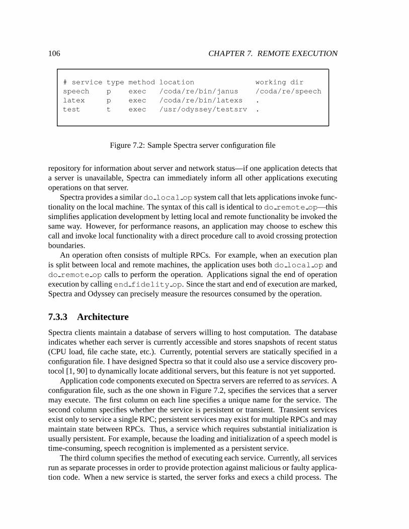
106 CHAPTER 7. REMOTE EXECUTION
# service type method location working dirspeech p exec /coda/re/bin/janus /coda/re/speechlatex p exec /coda/re/bin/latexs .test t exec /usr/odyssey/testsrv .
Figure 7.2: Sample Spectra server configuration file
repository for information about server and network status—if one application detects thata server is unavailable, Spectra can immediately inform all other applications executingoperations on that server.
Spectra provides a similar do local op system call that lets applications invoke func-tionality on the local machine. The syntax of this call is identical to do remote op—thissimplifies application development by letting local and remote functionality be invoked thesame way. However, for performance reasons, an application may choose to eschew thiscall and invoke local functionality with a direct procedure call to avoid crossing protectionboundaries.
An operation often consists of multiple RPCs. For example, when an execution planis split between local and remote machines, the application uses both do local op anddo remote op calls to perform the operation. Applications signal the end of operationexecution by calling end fidelity op. Since the start and end of execution are marked,Spectra and Odyssey can precisely measure the resources consumed by the operation.
7.3.3 Architecture
Spectra clients maintain a database of servers willing to host computation. The databaseindicates whether each server is currently accessible and stores snapshots of recent status(CPU load, file cache state, etc.). Currently, potential servers are statically specified in aconfiguration file. I have designed Spectra so that it could also use a service discovery pro-tocol [1, 90] to dynamically locate additional servers, but this feature is not yet supported.
Application code components executed on Spectra servers are referred to as services. Aconfiguration file, such as the one shown in Figure 7.2, specifies the services that a servermay execute. The first column on each line specifies a unique name for the service. Thesecond column specifies whether the service is persistent or transient. Transient servicesexist only to service a single RPC; persistent services may exist for multiple RPCs and maymaintain state between RPCs. Thus, a service which requires substantial initialization isusually persistent. For example, because the loading and initialization of a speech model istime-consuming, speech recognition is implemented as a persistent service.
The third column specifies the method of executing each service. Currently, all servicesrun as separate processes in order to provide protection against malicious or faulty applica-tion code. When a new service is started, the server forks and execs a child process. The

7.3. IMPLEMENTATION 107
service_init (&argc, &argv);while (1)
�
if (service_getop (&optype, &opid, path,&indata, &inlen) < 0)
�
return (-1);�
rc = run_latex (indata, inlen, &outdata, &outlen);
service_retop (opid, NULL, outdata, outlen);�
Figure 7.3: Sample service implementation
Spectra server uses two Unix pipes to communicate with the service.The last two columns in Figure 7.2 specify the location of the service executable and
the working directory in which it should be executed. Normally, service executables areplaced in the Coda file system. This simplifies deployment: any machine which is a Codaclient will execute the latest version of a service. As the last line shows, it is also possibleto execute services located on local file systems. However, the system maintainer is thenresponsible for ensuring consistency.
The Spectra server is multi-threaded, allowing it to accept multiple concurrent requests.Each RPC is handled by a separate thread, which routes the request to the appropriateservice. When a transient request is received, the server thread dynamically creates a newservice to handle the request. If a RPC requests a persistent service, the server threaddetermines if the specified service is currently running. If it is not running, the service canbe created on demand.
A persistent service may choose to handle multiple requests simultaneously. When aserver thread receives a RPC for a service, it assigns a unique identifier to the request andwrites the request to the service’s input pipe. When the service replies, it specifies theidentifier of the request to which it is replying.
Spectra provides an application library which simplifies service implementation. Fig-ure 7.3 shows the main loop of a simple service. The service init library functionparses the command line arguments and extracts Spectra-specific information, includingthe input and output pipes used to communicate with the Spectra server. In the main loop,the service calls service getop, which blocks until a request is received. The functionreturns the type of operation requested, a unique identifier associated with the request, andapplication-specific input data. The sample service has only one request type—servicesthat handle more than one request type multiplex on optype. When processing is com-

108 CHAPTER 7. REMOTE EXECUTION
init Initializes the monitor.term Called on termination.predict avail Predicts the amount of resources available
for operation execution.get measured cnt Returns the number of resources measured.start op Starts measuring resource usage for an operation.stop op Stops measuring resource usage. Returns the amount
of resource consumed.add usage Adjusts measurements to account for resources
consumed on a Spectra server.update predictions Refreshes the cached predictions of a
proxy monitor.
Figure 7.4: Resource monitor functions
plete, the service calls service retop, passing in the request identifier and application-specific output data.
7.3.4 Resource monitors
Spectra measures supply and demand for many different resources in order to make correctremote location decisions. This functionality is implemented as a set of resource monitors,code components that measure a single resource or a group of related resources. The re-source monitors are contained within a modular framework shared by Spectra clients andservers. In pervasive computing environments, it is difficult to anticipate what resourcesmight impact application execution—Spectra’s measurement framework makes it easy toadd new measurement capability. Further, the modular design allows one to implementseveral different methods of measuring a particular resource and choose the appropriatemethod for each particular execution environment.
Currently, Spectra’s implementation includes six types of monitors: CPU, network, bat-tery, file cache state, remote CPU, and remote file cache state. Each monitor provides thecommon set of functions shown in Figure 7.4. Prior to executing an operation, Spectragenerates a resource snapshot, which provides a consistent view of the local and remoteresources available for execution. Spectra first generates a list of servers that could possi-bly execute some portion of the operation; this list may include the local client machine.For each server in the list, Spectra iterates through the set of resource monitors, callingpredict avail. Each monitor returns predicted resource availability—for example,the network monitor returns predicted network bandwidth and latency for communicatingwith the specified server. The predictions in the snapshot are used to decide how and wherethe operation will execute.
During operation execution, the resource monitors observe application resource usage.Before executing an operation, Spectra calls start op, which alerts each monitor to be-

7.3. IMPLEMENTATION 109
gin observation. After the operation completes, Spectra calls stop op, which terminatesmeasurement and returns the amount of resources consumed. The add usage functionaccounts for resource usage on Spectra servers—the monitor adds reported resource con-sumption to the total resource usage of the operation.
Spectra logs measured resource consumption and creates models that predict futureresource demand. Thus, the more an operation is executed, the more accurately its resourceusage is predicted.
The CPU monitor
The CPU monitor predicts availability using a smoothed estimate of recent load. The mon-itor first determines the amount of competition for the local CPU by measuring the per-centage of CPU cycles recently used by other processes. It then calculates the percentageof cycles available for operation execution by assuming that background load will remainunchanged and that the operation will get a fair share of the CPU. It multiplies this valueby the processor speed to predict the number of CPU cycles per second the operation willreceive. Narayanan et al. [64] describe this prediction algorithm in more detail.
The monitor observes CPU usage by associating an operation with the identifier of theexecuting process. This distinguishes the CPU usage of concurrent operations. Beforeand after execution, the monitor observes CPU statistics for the executing process and itschildren using Linux’s /proc file system. It returns total cycles used by the operation.
The network monitor
The network monitor predicts network bandwidth and latency using an algorithm first de-veloped for Odyssey [68]. Predictions are based upon passive observation of communica-tion between the Spectra client and remote servers. The RPC package logs the sizes andelapsed times of short exchanges and bulk transfers. The short, small RPCs give an approx-imation of round trip time, while the long, large bulk transfers give an approximation ofthroughput. The network monitor periodically examines the recent transmission logs, anddetermines the instantaneous bandwidth available to the entire machine. It then estimateshow much of that bandwidth is likely to be available for communicating with each server,assuming that the first hop is the bottleneck link in the network. When the network monitoris queried, it returns the predicted latency and bandwidth available for communicating witha specified server.
Observing network usage is trivial since all client-server communication passes throughSpectra. Whenever an application performs a RPC, the network monitor records the numberof bytes sent and received. After the operation completes, the monitor returns total bytestransmitted, total bytes received, and the number of RPCs performed.

110 CHAPTER 7. REMOTE EXECUTION
The battery monitor
The implementation details of the battery monitor have already been described in Chap-ter 6. Each method of observing battery status and energy usage (Smart Battery, ACPI,and modulation) is implemented as a separate monitor. The modular design of the resourcemonitor framework makes it easy to select the appropriate measurement methodology whencompiling for different hardware platforms.
When asked to predict resource availability, the battery monitor returns the amountof energy remaining in the client’s battery (if the computer is currently battery-powered).It also returns the global feedback parameter, � , which represents the current importanceof energy conservation. During operation execution, the monitor observes energy usage.After the operation completes, it returns the total amount of energy consumed. Since itis difficult to distinguish the energy usage of concurrent operations, Spectra ignores datagathered from concurrently executed operations when modeling demand and predictingfuture energy needs.
The file cache state monitor
File cache state is an important resource in pervasive environments because data accessconsumes significant time and energy when items are unavailable locally. The file cachestate monitor estimates these costs by predicting which uncached objects will be accessedby an operation.
The file cache state monitor interacts with the Coda file system to predict cache state.Coda hides server access latency by caching files on clients. When the data accessed by anoperation is cached locally, the operation will take less time and consume less energy. Topredict this effect, the monitor asks Coda which files are in its cache. The monitor performsan ioctl on the Coda pseudo-device, which causes Coda to write a list of currently cachedfiles to a temporary file. Although it is possible that cache state will change slightly duringoperation execution, the changes are unlikely to be significant. The monitor also obtains anestimate of the rate at which uncached data will be fetched from file servers.
During operation execution, the monitor observes Coda file accesses by listening to aspecial Unix port. Upon operation completion, the monitor returns the names and sizes ofaccessed files. This method does not yet support concurrent operations. However, a similarapproach to that used by the CPU monitor could be used if Coda were to associate a processidentifier with each file access. Section 7.3.6 describes how this list of file accesses is usedto predict which files will be accessed during future operations.
The remote proxy monitors
Resource monitors on Spectra servers measure remote resource state. They communicatethis information to remote proxy monitors running on Spectra clients. Currently, Spectraservers execute local CPU and file state monitors, which communicate with remote CPUand file cache state proxy monitors on clients.

7.3. IMPLEMENTATION 111
Prior to operation execution, each proxy monitor predicts resource availability on serversthat could be used for execution. The proxy monitors cache availability information to im-prove performance. If a server has recently reported availability, the proxy returns thecached value. Otherwise, the proxy queries the server dynamically. The staleness thresholdis resource-specific—I currently use a one minute timeout for both CPU and file cache data.
Spectra periodically polls servers to determine if they are active. When a server sendsa positive acknowledgment, it also returns its resource snapshot, which includes the avail-ability of all measured resources. Upon receiving a snapshot, the Spectra client calls theupdate predictions function of each proxy monitor. This process lets Spectra updatethe resource status of servers that are not in active use.
When Spectra executes a remote RPC, server monitors observe resource usage andreport the total resource consumption as part of the RPC response. The Spectra client passesthis data to proxy monitors by calling their add usage functions. The proxy monitorsaccumulate server resource consumption and report the total when the operation completes.
7.3.5 Predicting resource demand
Spectra uses measurements of application resource usage to generate models that predictfuture demand. It assumes that the resources consumed by an operation will be similar tothose consumed by recent operations of similar type.
Spectra provides default predictors that model resource demand. For numerical datasuch as CPU and energy consumption, Spectra’s default predictor generates simple linearmodels of application behavior. The default file predictor is somewhat more complicated,and is described in the next section. We believe that Spectra’s default predictors will provesufficient for most applications; in fact, we use them for all current Spectra applications.However, we also recognize that some applications may require more complex predictorsto generate accurate predictions. Spectra therefore provides an interface through whichapplication-specific predictors can be specified.
When an application calls register fidelity, Spectra creates predictors for eachresource type. Each predictor reads the logged resource usage data and generates a pa-rameterized model of demand that is stored in memory. When subsequent operations areperformed, Spectra updates the in-memory model in addition to logging resource usage.
Each model predicts resource demand as a function of application fidelity and operationinput parameters. Fidelities and input parameters may be either discrete or continuous. Thedefault predictor uses binning to model discrete variables: it maintains a separate predictionfor each possible discrete value. The default predictor also maintains a generic predictionthat is independent of any discrete variable—this prediction is used whenever a specificcombination of discrete variables has not yet been encountered. The default predictor useslinear regression to model continuous variables. It adjusts for changes in application be-havior over time by giving more recent samples a greater weight in its predictions.
For some applications, resource usage depends heavily upon the specific data on whichan operation is performed. For example, the input document to the Latex document prepa-

112 CHAPTER 7. REMOTE EXECUTION
ration system will significantly affect resource usage: a 100 page document consumes moreCPU cycles and battery energy than a 2 page document.
Spectra’s default predictor anticipates this relationship with data-specific models of re-source usage. Applications such as Latex associate each operation with the name of adata object. The default predictor maintains a LRU cache of the most recent data objects.When asked to predict future demand, the predictor uses a data-specific model to predictresource usage if it finds such a model in its cache. Otherwise, it uses the more general,data-independent model. The size of the LRU cache is a parameter specified by applica-tions.
7.3.6 Ensuring data consistency
Since Coda relaxes data consistency under poor network conditions to achieve acceptableperformance, Spectra must interact with Coda to ensure that remotely-executed operationsread the same data that they would have read if they had been executed locally. This isvital for applications such as compilers and document processors that read files commonlymodified on clients.
Prior to executing an operation, Spectra predicts which files are likely to be accessed.Spectra provides a default file predictor that builds upon the numerical predictor describedin the previous section. In essence, the file predictor maintains a numerical prediction ofaccess likelihood for each file that may be accessed by an operation. When updating eachfile’s model, the file predictor assigns the value of 1 to a file access, and the value of 0 whena file is not accessed. Each resulting prediction thus represents the likelihood that a givenfile will be accessed.
Spectra uses the file predictor to estimate the cost of servicing cache misses. It comparesthe list of files that may be accessed by an operation to the list of cached files. For eachuncached file, it estimates the number of bytes of data that must be fetched from file serversby multiplying the file size by the predicted access likelihood. Summing this value overall files that may be accessed yields a prediction for the total number of bytes that must befetched to perform an operation. Spectra divides this prediction by the rate at which Codawill service cache misses to estimate the total amount of time that will be spent servicingcache misses.
Spectra uses the file predictor to maintain data consistency. Before executing an opera-tion remotely, Spectra ensures that all modifications to files with non-zero access likelihoodhave been reintegrated to file servers. Spectra also ensures that modifications made duringthe remote execution of an operation are immediately visible to the client. The file cachestate monitor provides a list of files accessed during an operation. The Spectra serverreintegrates all local modifications to those files and delays its reply to the RPC until thereintegration completes.
If a large amount of data must be reintegrated in poor network conditions, then dataconsistency significantly increases remote operation execution time. Spectra estimates theadded execution time before deciding where to execute an operation. It calculates the

7.3. IMPLEMENTATION 113
reintegration cost by multiplying the size of the modifications by the predicted bandwidthavailable to the file server. If the predicted reintegration costs are too high, Spectra avoidsthem by executing the operation locally.
7.3.7 Selecting the best option
When applications call begin fidelity op, Spectra selects a location and fidelity atwhich to perform the operation. It first determines which servers could possibly executethe operation. Then, Spectra and Odyssey poll the resource monitors to obtain a snapshotof resource availability on the client and potential remote servers. Finally, the Odysseymulti-fidelity solver, described in Section 6.2.4, is used to decide how and where to executethe operation. The server selects the alternative that maximizes an input utility function.Because it uses search heuristics, it is not guaranteed to select the optimal alternative—however, as the results in Section 7.4 show, it usually selects a very good option.
Spectra provides a default utility function that has so far proven sufficient for all Spec-tra applications. As with Spectra predictors, applications may override the default utilityfunction with an application-specific implementation. The default utility function evaluatesexecution alternatives by their impact on user metrics. User metrics measure performanceor quality perceptible to the end-user—they are thus distinct from resources, which are notdirectly observable by the user (other than by their effect on metrics). Spectra currentlyconsiders three user metrics: execution time, energy usage, and application fidelity.
A utility function represents a specific characterization of the desirability to the userof each possible alternative for execution. If the utility function poorly characterizes userpreferences, then the alternative selected by Spectra may not be the most desirable (evenwhen it maximizes the utility function). In my evaluation of Spectra, I assume that the util-ity function represents a good characterization of user preferences. A qualitative evaluationof the results in Section 7.4 suggests that the default utility function produces a reasonableapproximation of user preferences—the choices made by Spectra appear to be correct.
As the solver searches the space of possible alternatives, it calls the utility functionwith specific input parameters, fidelities, execution plans, and server choices. To evaluateeach alternative, the default utility function first predicts a context-independent value foreach metric: total execution time, total energy usage, and a vector representing applicationfidelity. It then weights each value by how important it currently is to the user. It returnsthe product of the weighted values as the utility of the alternative.
The default utility function predicts execution time to be the sum of local and remoteCPU time, network transmission time, time to service cache misses, and time to ensure dataconsistency. This simple model reflects Spectra’s current implementation, which does notallow computation and network transmission to overlap.
The utility function uses the models of operation resource usage described in Sec-tions 7.3.5 to predict resource demand. It matches demand to the prediction of resourceavailability contained in the resource snapshot. It calculates local CPU time by dividingthe predicted cycles needed for execution by the predicted amount of cycles per second

114 CHAPTER 7. REMOTE EXECUTION
available on the local machine. Remote CPU time is calculated similarly. Network trans-mission time is calculated by predicting the number of bytes to be transmitted and dividingby the available bandwidth. Spectra then adds the affect of latency by multiplying the pre-dicted number of round trips by the round-trip time. Spectra calculates the time to servicefile cache misses and ensure data consistency as described in the previous section.
The importance of execution time is application-specific. Therefore, Spectra requireseach application to provide a function that expresses the desirability of different latencyvalues. Many Spectra applications use the simple expression,
� ���where T is the predicted
execution time. This has the nice property that an operation that takes twice as long toexecute is only half as desirable to the user.
The default utility function predicts energy consumption using the history of past ap-plication energy usage, as described in Section 6.2.3. Spectra weights the importance ofenergy conservation by using goal-directed adaptation. The weighted energy component ofutility is calculated as
� � � � ��� �, where
�is predicted energy usage, � is the global feedback
parameter, and � is a constant (currently set to 10). The exponential function allows � to actas a weighting factor—high values of � cause energy usage to be the dominant componentof the utility calculation. Thus, when � is 0, energy usage does not impact utility at all, andwhen � is 1, energy usage has a very large impact. The value of � limits the maximum im-pact of energy usage on the utility calculation. Higher values of � make energy usage moredominant when energy conservation is extremely critical, but make the utility calculationvery sensitive to slight changes in the value of � when energy conservation is less critical. Ihave set the value of � to 10 to balance these concerns.
Fidelity is a multidimensional metric of application-specific quality. Since fidelity isfixed as an input to the utility function, no prediction is necessary. However, each applica-tion must provide a function which specifies the desirability of each fidelity as a numericalvalue. Spectra’s default utility function calls the provided function to obtain the application-specific desirability of the input fidelity.
7.3.8 Applications
Three applications have been modified to use Spectra: the Janus speech recognizer, theLatex document preparation system, and the Pangloss-lite natural language translator [24].I modified the first two applications, while Pangloss-lite was modified by SoYoung Park.
Speech recognition
The Janus speech recognizer was previously described in Section 4.5. It has three possibleexecution plans: local, hybrid, and remote. It also supports two fidelities: full-quality andreduced-quality recognition. Janus assigns reduced-quality recognition the value 0.5, andfull-quality recognition the value 1.0. For execution time, Janus specifies that utility isinversely proportional to the expected latency.
The speech recognizer can use a task-specific vocabulary to recognize utterances in aparticular context. Since the choice of vocabulary influences resource usage, Janus specifies

7.3. IMPLEMENTATION 115
the vocabulary name when executing an operation–this allows Spectra to generate data-specific predictions for recently used vocabularies. Since the data files accessed by Janusare typically static, there are no data consistency issues for the application.
Document preparation
The Latex document preparation system generates a graphical DVI file from multiple inputfiles. Latex only has a single fidelity, since documents must typically be generated at high-est quality. The application has two possible execution plans: local, in which all processingis done on the client, and remote, in which all processing is done on a remote server. Aswith Janus, Latex specifies that utility is inversely proportional to the expected latency.
I have modified Latex to use Spectra by creating two minimal code components: afront-end and a Spectra service. The front-end calls Spectra to select an execution location.It specifies the name of the top-level input file so Spectra can parameterize its predictionsby document. The service runs Latex as a child process when requested.
Data consistency is a significant consideration when executing Latex. The user willoften have locally modified one or more input files. Spectra must ensure that any modifica-tions are reintegrated before processing is done remotely,
Natural language translation
Pangloss-Lite translates text from one language to another. It can use up to three transla-tion engines: EBMT (example-based machine translation), glossary-based, and dictionary-based. Each engine returns a set of potential translations for phrases contained within theinput text. A language modeler combines the output of the engines to generate the finaltranslation.
Pangloss-Lite fidelity increases with the number of engines used for translation. Sincethe EBMT engine has the largest data set, it is assigned a fidelity of 0.5. The glossary-basedand dictionary-based engines produce subjectively worse translations—they are assignedfidelity levels of 0.3 and 0.2, respectively. When multiple engines are used, their respectivefidelities are added since the language modeler can combine their outputs to produce abetter translation. For example, when the EBMT and glossary-based engines are used, afidelity of 0.8 is assigned.
For Pangloss-Lite, any execution that takes longer than 5 seconds is undesirable—i.e.,the execution component of the utility function assigns it a value of 0. Conversely, alltranslations that take less than half a second are equally good; they are assigned a utilityvalue of 1. Translations that take time, T, between one half and five seconds are assignedutility
� � � ���� � � � � � ���� � .All three translation engines and the language modeler may be executed remotely.
While execution of each translation engine is optional, the language modeler must alwaysbe executed. Thus, there are 54 separate execution plans from which Spectra may choose.Pangloss-Lite seldom modifies its data files, so data consistency is of little concern.

116 CHAPTER 7. REMOTE EXECUTION
Baseline Energy Network CPU File cache0
50
100
Exe
cutio
n T
ime
(sec
onds
)
Local / ReducedLocal / FullHybrid / ReducedHybrid / FullRemote / ReducedRemote / FullSpectra
S S S S
S
This figure shows speech recognition execution time for the five resource scenarios de-scribed in Section 7.4.1. Each data set represents a different scenario. The first six barsshow the execution time for each possible combination of execution plan and fidelity. Ineach data set, the alternative selected by Spectra is marked with a “S”. The final bar ineach data set shows execution time when Spectra is used to select the best alternative.Each bar represents the mean of five trials—the error bars show 90% confidence intervals.
Figure 7.5: Speech recognition execution time
7.4 Validation
My validation of Spectra measured how well Spectra adapts to changes in resource avail-ability. I executed Janus, Latex, and Pangloss-Lite under a variety of scenarios in which Ivaried resource availability. For each scenario, I measured application latency and energyusage for each possible combination of fidelity, execution plan, and server choice. I alsoasked Spectra to choose one of the possible alternatives for application execution. If Spec-tra chose the best possible alternative, I considered the outcome successful; otherwise, Iconsidered it a failure. The results of this validation are shown in the next three sections.Section 7.4.4 provides a more detailed evaluation of the overhead of Spectra execution.
7.4.1 Speech recognition
For the speech recognition validation, I limited possible execution to two machines. Theclient machine, an Itsy v2.2 pocket computer, represents the type of small, highly-mobiledevices used for pervasive computing. Spectra used the Smart Battery energy monitor tomeasure Itsy energy usage. An IBM T20 laptop with a 700 MHz Pentium III processor and256 MB DRAM served as a possible remote server. Since the Itsy lacks a PCMCIA slot

7.4. VALIDATION 117
Energy0
10
20
30
40
Ene
rgy
(Jou
les) Local / Reduced
Local / FullHybrid / ReducedHybrid / FullRemote / ReducedRemote / FullSpectra
S
This figure shows speech recognition energy usage for the energy resource scenario de-scribed in Section 7.4.1. The first six bars show energy usage for each possible combi-nation of execution plan and fidelity. Spectra selected the Remote / Full alternative, soit is marked with a “S”. The final bar shows energy usage when Spectra is used to selectthe best alternative. Each bar represents the mean of five trials—the error bars show 90%confidence intervals.
Figure 7.6: Speech recognition energy usage
(such as is available on the Compaq iPAQ handheld), the two machines were connectedwith a serial link.
I first recognized 15 utterances so that Spectra could learn the application’s resourcerequirements. I then measured how well Spectra performed when recognizing a new utter-ance in five different resource scenarios.
Figure 7.5 shows measured execution time for each scenario. The first data set showsresults for the baseline scenario, in which both computers have no significant CPU activityand are connected to wall power. The first six bars show execution time for each alternativeavailable to Spectra. The local execution plan is clearly inferior to the hybrid and remoteplans, taking 3–9 times as long to execute. The large disparity is caused by the speech rec-ognizer’s substantial use of floating-point instructions, which are emulated in software onthe Itsy’s StrongArm processor. However, using the hybrid execution plan and performingsome computation locally takes less time than using the remote execution plan.
The “S” label in each scenario in Figure 7.5 indicates which alternative was chosen bySpectra. In the baseline scenario, Spectra correctly chooses the hybrid execution plan andfull vocabulary. This combination takes less time to execute than all but one alternative.The quicker alternative executes only slightly faster, but has a fidelity only half as desirable

118 CHAPTER 7. REMOTE EXECUTION
Baseline File cache Reintegrate Energy0
2
4
6
Exe
cutio
n T
ime
(sec
onds
) Local Remote ARemote BSpectra
SS
S
S
This figure shows Latex execution time when preparing a 14-page document in each ofthe four resource scenarios described in Section 7.4.2. Each data set represents a differ-ent scenario. The first three bars show the execution time for each possible executionlocation—the location selected by Spectra is marked with a “S”. The final bar in each dataset shows execution time when Spectra is used to select the best alternative. Each barrepresents the mean of five trials—the error bars show 90% confidence intervals.
Figure 7.7: Latex execution time for the small document
to the user. The last bar in each data set shows the execution time when Spectra choosesthe best alternative—the difference in height between this bar and the one indicated withan “S” shows Spectra’s decision overhead. In all scenarios the overhead is minimal—thedifference in height is within the 90% confidence intervals.
Each remaining scenario differs from the baseline by varying the availability of a singleresource. In the energy scenario, the client is battery-powered with an ambitious batterylifetime goal of 10 hours. The second data set in Figure 7.5 shows latency results for thisscenario, and Figure 7.6 shows measured energy usage. Since energy conservation is crit-ical, Spectra chooses the remote execution plan and the full vocabulary. Although hybridexecution takes less time, it consumes more energy because a portion of the computationis done on the client. As in the baseline scenario, Spectra correctly chooses to avoid thereduced vocabulary—the small energy and latency benefits do not outweigh the decreasein fidelity.
The network scenario halves the bandwidth between the client and server. This makesremote execution especially undesirable, and Spectra correctly chooses to use the hybridexecution plan and full vocabulary. The CPU scenario loads the client processor by exe-cuting a CPU-intensive background job. The cost of local computation increases, makingthe remote execution plan more attractive. Spectra chooses the remote plan because the
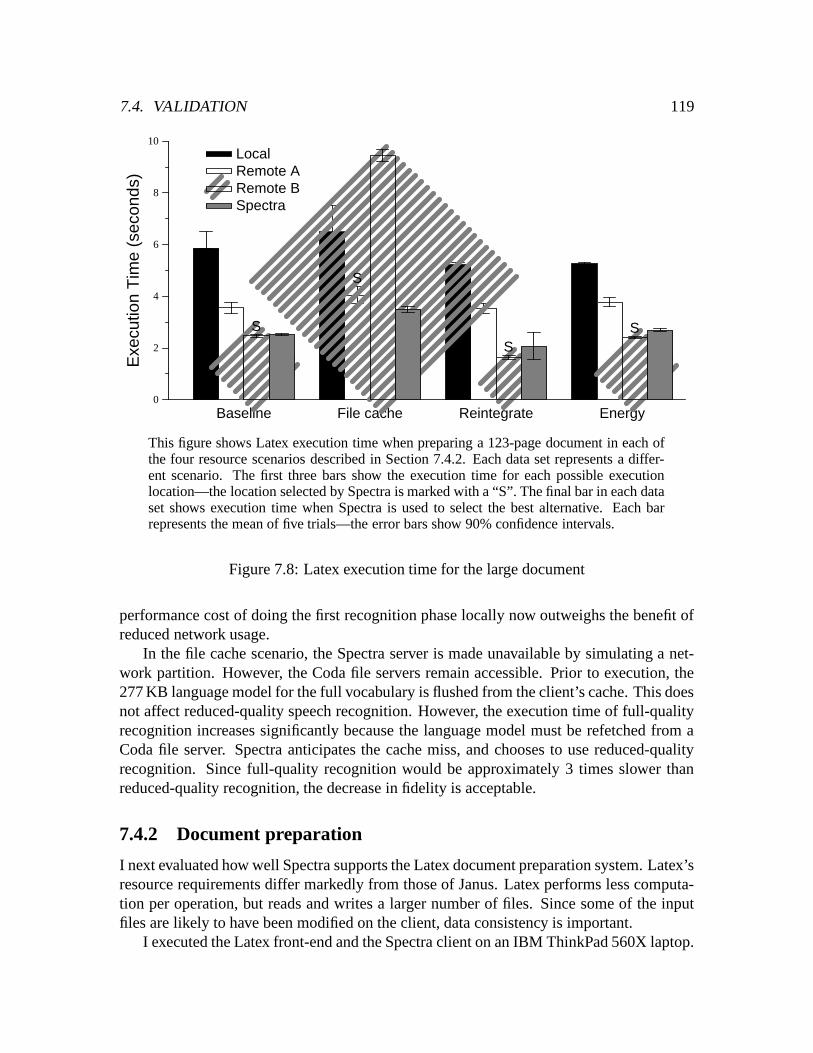
7.4. VALIDATION 119
Baseline File cache Reintegrate Energy0
2
4
6
8
10E
xecu
tion
Tim
e (s
econ
ds)
Local Remote ARemote BSpectra
S
S
SS
This figure shows Latex execution time when preparing a 123-page document in each ofthe four resource scenarios described in Section 7.4.2. Each data set represents a differ-ent scenario. The first three bars show the execution time for each possible executionlocation—the location selected by Spectra is marked with a “S”. The final bar in each dataset shows execution time when Spectra is used to select the best alternative. Each barrepresents the mean of five trials—the error bars show 90% confidence intervals.
Figure 7.8: Latex execution time for the large document
performance cost of doing the first recognition phase locally now outweighs the benefit ofreduced network usage.
In the file cache scenario, the Spectra server is made unavailable by simulating a net-work partition. However, the Coda file servers remain accessible. Prior to execution, the277 KB language model for the full vocabulary is flushed from the client’s cache. This doesnot affect reduced-quality speech recognition. However, the execution time of full-qualityrecognition increases significantly because the language model must be refetched from aCoda file server. Spectra anticipates the cache miss, and chooses to use reduced-qualityrecognition. Since full-quality recognition would be approximately 3 times slower thanreduced-quality recognition, the decrease in fidelity is acceptable.
7.4.2 Document preparation
I next evaluated how well Spectra supports the Latex document preparation system. Latex’sresource requirements differ markedly from those of Janus. Latex performs less computa-tion per operation, but reads and writes a larger number of files. Since some of the inputfiles are likely to have been modified on the client, data consistency is important.
I executed the Latex front-end and the Spectra client on an IBM ThinkPad 560X laptop.

120 CHAPTER 7. REMOTE EXECUTION
Energy0
10
20
30
40
Ene
rgy
(Jou
les)
Local Remote ARemote BSpectra
S
This figure shows Latex energy usage when preparing a 14-page document in the energyresource scenario described in Section 7.4.2. The first three bars show energy usage foreach possible execution location. Spectra selected Remote B, so that alternative is markedwith a “S”. The final bar shows energy usage when Spectra is used to select the bestlocation. Each bar represents the mean of five trials—the error bars show 90% confidenceintervals.
Figure 7.9: Latex energy usage for the small document
I ran Spectra servers on the laptop and on two remote servers; server A had a 400 MHzPentium II processor, server B had a more powerful 933 MHz Pentium III processor. Thus,there are three possible alternatives: local execution on the laptop, remote execution onserver A, and remote execution on server B. The laptop communicated with the serversusing a 2 Mb/s 2.6 GHz wireless WaveLAN network.
I used two documents for evaluation: the smaller document was 14 pages in length, andthe larger was 123 pages. I first executed Latex 10 times on each document to allow Spectrato learn application resource requirements. I then measured how well Spectra performedwhen preparing the documents in four different resource scenarios.
Figure 7.7 shows the measured execution time for preparation of the smaller document.The first data set shows the baseline scenario, in which all computers have no significantCPU activity and are connected to wall power. All files needed for document preparationare cached on every machine. Since little data is transmitted over the network, CPU speedis the primary consideration in this scenario. Remote execution proves faster than localexecution, with server B preparing the document more quickly than server A due to itsfaster processor. As shown by the “S” above the third bar, Spectra chooses to use serverB. The fourth bar in the data set shows that the time used by Spectra to choose the correct

7.4. VALIDATION 121
Energy0
20
40
60
Ene
rgy
(Jou
les)
Local Remote ARemote BSpectra
S
This figure shows Latex energy usage when preparing a 123-page document in the energyresource scenario described in Section 7.4.2. The first three bars show energy usage foreach possible execution location. Spectra selected Remote B, so that alternative is markedwith a “S”. The final bar shows energy usage when Spectra is used to select the bestlocation. Each bar represents the mean of five trials—the error bars show 90% confidenceintervals.
Figure 7.10: Latex energy usage for the large document
execution plan is minimal. Figure 7.8 shows similar results for the larger document.In the file cache scenario, server B does not have any document input files cached
locally. The execution of Latex is delayed while it fetches files from the server. Figures 7.7and 7.8 show that file cache misses greatly increases the time needed to execute Latex onserver B. Spectra correctly anticipates this and switches execution to server A for bothdocuments.
In the reintegrate scenario, a 70 KB input file for the smaller document is modified onthe client. Before preparing the smaller document on a remote server, Spectra must ensurethat the modified input file is reintegrated to the file servers. As Figure 7.7 shows, rein-tegration over the wireless network significantly increases execution time for both remoteexecution options. Since the modification already exists on the client, the speed of localexecution is unaffected. Spectra therefore chooses to use the local execution plan for thesmaller document.
The modified source file is not an input for the larger document. As Figure 7.8 shows,Spectra predicts that the modified file will not be needed and does not force reintegration.Spectra therefore chooses the fastest plan: execution on server B. In this scenario, data-specific prediction allows Spectra to choose the fastest execution plan for each document.

122 CHAPTER 7. REMOTE EXECUTION
Baseline File cache CPU0
20
40
60
80
100
Per
cent
ile
11 words23 words35 words47 words59 words
This figure shows the accuracy of Spectra’s choices for how and where to executePangloss-Lite operations. It shows results for five different sentences translated in threeresource scenarios. In each case, the 100 possible alternatives available to Spectra areranked by their utility—the height of each bar gives the percentile into which Spectra’schoice falls. Thus, a height of 99 indicates that Spectra’s choice is in the 99th percentile.Each bar represents the mean of five trials. The error bars show 90% confidence intervals.
Figure 7.11: Accuracy of Spectra choices for Pangloss-Lite
The energy scenario is identical to the reintegrate scenario, except that the client isdisconnected from wall power and a very aggressive goal for battery lifetime is specified.For the smaller document, Spectra chooses server B, even though this takes more time toexecute. Figure 7.9 shows the reason for this choice: remote execution on server B usesslightly less energy than the other options. Because energy is of paramount concern due tothe aggressive battery goal, Spectra opts for energy savings over a smaller execution time.The choice for the larger document is much clearer, since execution on server B saves bothtime and energy.
7.4.3 Natural language translation
I evaluated Pangloss-Lite using the same experimental setup as for Latex—this evaluationwas performed with the help of SoYoung Park. I translated a set of 129 sentences fromSpanish to English to allow Spectra to learn application resource requirements. I thenasked Spectra to choose the best option for translating five additional sentences of differentlength from Spanish to English.
Pangloss-Lite has more alternatives for execution than either previous application—Spectra may choose from 100 different combinations of location and fidelity. Due to the

7.4. VALIDATION 123
Baseline File cache CPU0.0
0.2
0.4
0.6
0.8
1.0R
elat
ive
Util
ity11 words23 words35 words47 words59 words
This figure shows the utility of using Spectra to choose how and where to executePangloss-Lite operations. It shows results for five different sentences translated in threeresource scenarios. Each bar shows the ratio of the utility when Spectra chooses an alter-native to the utility achieved when an oracle with no overhead makes the optimal choice.Thus, the ideal height of 1.0 indicates that Spectra has made the best possible choice andincurred no overhead. Each bar represents the mean of five trials—the error bars show90% confidence intervals.
Figure 7.12: Relative utility of Spectra choices for Pangloss-Lite
large number of alternatives, the results are presented in a different format. I rank thealternatives by the utility they achieved. Each bar in Figure 7.11 shows the percentile intowhich Spectra’s chosen alternative falls. A value of 99 indicates that Spectra has made anoptimal choice, while a value of 0 indicates that Spectra has made the worst possible choice.Each bar in Figure 7.12 compares the utility achieved when Spectra is used to choose analternative to the optimal utility that would be achieved if an oracle with no overhead chosethe best possible alternative. Even when Spectra chooses the optimal alternative, it usuallywill not achieve a ratio of 1.0 because its overhead increases overall translation time.
In the baseline scenario, all computers have no significant CPU activity, are connectedto wall power, and have all data files cached. For the three smallest sentences, Spectraexecutes all three translation engines. For the two larger sentences, Spectra does not ex-ecute the glossary-based engine. Its choice of which engines to execute is optimal for allsentences. This scenario shows the importance of modeling operation input parameters—Spectra correctly predicts that execution time will increase with sentence size and switchesto a lower fidelity to achieve acceptable performance for larger sentences.
Spectra runs the dictionary-based engine locally for the four smallest sentences and ex-ecutes all other components on server B. Remote execution yields significant performance

124 CHAPTER 7. REMOTE EXECUTION
improvements for the glossary-based and EBMT engines because they have large CPU re-quirements. The location of the dictionary-based engine and the language modeler does notaffect performance much because their processing requirements are small. Thus, althoughSpectra’s location choice for these two components is not optimal for all sentences, theperformance penalty is small (less than 0.07 seconds).
The baseline scenario illustrates an important property of Spectra. When alternativeshave significant difference in utility, Spectra almost always makes the correct decision. Ifit does choose an alternative that is not best, the utility of its choice is usually very close tooptimal. For the five sentences in the baseline scenario, the utility of Spectra’s choices areall within 2% of optimal. Even adding in the overhead of picking the correct alternative, asshown in Figure 7.12, the utility of Spectra’s choices are all within 7% of optimal.
In the file cache scenario, a 12 MB file needed by the EBMT engine was not in serverB’s cache. This made execution of the EBMT engine prohibitively slow on server B. Spec-tra therefore chose to use server A for remote execution in this scenario. Spectra executedall engines for the smallest sentence, but did not execute the glossary-based engine for theothers. Because server A is slower than server B, the application more quickly reaches thecrossover point where the the fidelity benefit of executing the glossary-based engine is lessthan the performance cost.
As with the baseline scenario, Spectra’s choices of which engines to execute are op-timal. While it chooses the correct location to execute the glossary-based and EBMTengines, it sometimes incorrectly places the dictionary-based engine and language mod-eler. However, the performance impact of these incorrect location decisions is less than0.1 seconds for all sentences. With decision overhead, the utilities achieved by Spectra arewithin 7% of optimal.
In the CPU scenario, I varied the file cache scenario by executing two CPU-intensiveprocesses on server A. This proved to be an interesting scenario, since the optimal choiceof server and engines to execute was different for each sentence. For the 11 and 35 wordsentences, Spectra’s only mistake was in locating the language modeler, and it achievedutility within 5% of optimal. For the 23 word sentence, Spectra made an optimal choice infour of five trials, but chose the incorrect server in one trial, leading to the high varianceshown in Figure 7.12. For the 47 word sentence, Spectra consistently chose to use server Awhen server B was optimal, and consequently achieved utility only 55% of optimal—thiswas the worst decision made by Spectra in any of our experiments. For the largest sentence,Spectra incorrectly chose to execute the glossary-based and dictionary-based engines infour trials when the combination of EBMT and dictionary-based engines was best.
In general, Spectra did an excellent job of choosing the best alternative for Pangloss-Lite execution. On average, it achieved 91% of the optimal utility.
7.4.4 Overhead
I measured Spectra’s overhead by performing a null operation, one which returns immedi-ately after being invoked. Figure 7.13 shows the amount of time needed to execute the null

7.4. VALIDATION 125
Activity No Servers 1 Server 5 Servers
register fidelity op 1.2 ms. 1.5 ms. 1.2 ms.begin fidelity op 8.3 ms. 13.1 ms. 65.5 ms.
file cache prediction�
5.2 ms. 8.5 ms. 8.5 ms.other resource prediction 0.8 ms. 1.6 ms. 7.2 ms.choosing an alternative 0.4 ms. 1.0 ms. 43.4 ms.other activity 1.9 ms. 2.0 ms. 6.4 ms.
do local op 5.9 ms. 4.7 ms. 5.1 ms.operation execution 4.9 ms. 4.0 ms. 4.0 ms.other activity 1.0 ms. 0.7 ms. 1.1 ms.
end fidelity op 2.1 ms. 2.1 ms. 2.2 ms.
total 18.4 ms. 21.4 ms. 74.0 ms.
This figure shows the amount of time Spectra takes to perform a null operation. The threecolumns show the amount of time spent on each activity when 0, 1, and 5 remote serversare available for execution. The times shown represent the mean of ten trials. This figureshows results for a relatively small local file cache (less than 100 files); for a full cache,measured time for file cache prediction is 359.6 ms.
Figure 7.13: Spectra overhead
operation when Spectra has 0, 1, and 5 remote servers on which it can choose to locate theoperation.
With no remote servers are available, the null operation takes 18 ms. to execute. Themajority of this time is spent in the begin fidelity op and do local op systemcalls. File cache prediction takes 5.2 ms. with a relatively empty cache; however, it cantake as long as 359.6 ms. when the file cache is full. The excessive overhead of file cacheprediction is due to the inefficient file system interface—every time a prediction is needed,Coda writes the entire cache state to a temporary file. If Spectra replaced this interface withone that sends incremental updates through a Unix socket whenever files are evicted from oradded to the cache, then the overhead of file prediction would be much less. The executionof the local operation takes 4.9 ms., mostly due to the cost of inter-process communication.
Spectra’s overhead increases with the number of potential servers. As Figure 7.13shows, the primary reason for the additional overhead is the time taken to choose the bestalternative. With each additional server, Spectra has more possible alternatives from whichto choose. However, total Spectra overhead is only 74 ms. with five servers, which is veryreasonable for the targeted set of applications—those that perform operations of a secondor more in duration.

126 CHAPTER 7. REMOTE EXECUTION
7.5 Summary
Remote execution is an important dimension of energy-aware adaptation. Applicationscan execute part of their functionality on remote servers to reduce their consumption ofbattery energy on a client machine. However, the goal of reducing energy consumptionwill often conflict with competing goals such as reducing execution time and maintaininghigh application fidelity.
Spectra provides the necessary system support to help applications arbitrate betweenthese competing goals. Spectra is designed for pervasive environments: it predicts theavailability of battery energy, file cache state, network bandwidth, and CPU cycles. It alsoobserves application resource usage to predict future needs. Using these predictions, itevaluates possible locations and fidelities for execution, and advises applications how andwhere they can best execute operations.
Evaluation of Spectra using a speech recognizer, a document preparation system, and anatural language translator shows that Spectra often chooses the best location and fidelityfor execution despite wide variation in resource availability. When Spectra does not makethe best decision, its choice is usually very close to optimal. Further, the overhead of thesystem is reasonable for applications which perform remote operations of a second or morein duration.

Chapter 8
Related work
This dissertation is one of the first comprehensive efforts to address higher-level energymanagement. To the best of my knowledge, it includes several novel contributions:
� It has described the design and implementation of PowerScope, the first tool to useprofiling to map energy consumption to program structure.
� It has shown that applications can modify their behavior to conserve significantamounts of energy when battery levels are critical. The key method of conservationis reduction of application fidelity.
� It has demonstrated that the operating system can effectively manage energy as aresource and meet user-specified goals for battery lifetime.
� It has shown how system support for remote execution can enable applications todynamically balance the competing goals of energy conservation, performance, andhigh fidelity.
While there is no single research effort which spans all the subjects discussed in thisdissertation, there is a large amount of work that intersects one or more areas. In this chap-ter, I discuss work related to each part of the dissertation. The next section describes otherapproaches to energy measurement. Section 8.2 describes related work in energy manage-ment, dividing this topic into efforts aimed at the higher levels of the system and effortsaimed at hardware devices. Section 8.3 summarizes the most relevant work in adaptiveresource management, and Section 8.4 describes work related to Spectra.
8.1 Energy measurement
While PowerScope is the first energy profiler, its development was aided by previous workin CPU profiling. In particular, the implementation of the System Monitor is closely relatedto similar sampling-based profilers designed to run continuously, such as Morph [100] andDCPI [3].
127

128 CHAPTER 8. RELATED WORK
Other than the profiling technique used by PowerScope, there are two main approachesto measuring application energy usage. The first approach, which I shall refer to as energyaccounting, measures the energy consumption of specific system activities. Then, whenapplications execute, the energy accounting tool counts the number of times each activityoccurs. By multiplying the number of occurrences by the energy usage per activity, the toolestimates total application energy usage.
PowerMeasure and StateProfiler, developed by Lorch and Smith [53, 54], provide en-ergy measurements for Apple Macintosh PowerBook Duo laptops. PowerMeasure bench-marks the power expended by hardware components such as the disk and CPU while theyoperate in various power states. For example, it measures the power expended by the harddisk when it is spinning and when it is idle. During application execution, StateProfilerrecords transitions between power states and uses the benchmark data to estimate total en-ergy consumption. The tools report average power usage and total energy expended byeach hardware component.
The Millywatt tool, developed by Cignetti et al. [11], estimates energy usage for ap-plications executing on PalmOS handheld computers. The tool models power usage foreach hardware device state, as well as the cost of transitioning between states. When ap-plications are executed in a modified simulator, the tool traps system calls to infer whentransitions occur between device power states. From this information, the tool estimatesthe energy usage of the simulated application.
Neugebauer and McAuley propose to incorporate energy accounting into the Neme-sis operating system [66]. They observe that Nemesis already provides accurate resourceaccounting of traditional resources such as CPU, network, display, and disk. Bellosa [5]performs energy accounting using CPU performance counters. He proposes counting thenumber of total instructions executed, number of floating-point instructions, and number ofcache misses to estimate the amount of energy consumed by the CPU and memory subsys-tem.
Energy accounting has several drawbacks. First, correct accounting relies on the com-pleteness of the energy model. The model developer must benchmark every hardware de-vice that may be a significant source of power consumption. The model must also includeall possible power states and transition costs for each device. This means that developingan accurate model is non-trivial. Further, a new model must be developed for each hard-ware platform on which energy measurements are needed. The second drawback is thataccounting does not capture variance in power expenditure within a single state. For ex-ample, CPU power usage varies with the instruction mix [87] and wireless network powerusage varies with the amount of channel congestion [77]. Finally, it is difficult to imagineexpending this approach to capture the effects of power management performed entirely inhardware, such as the 802.11 standard for wireless networks. One significant advantage ofenergy accounting is that it can separate out the energy consumption of asynchronous ac-tivities such as disk spin-up which PowerScope assigns to the currently executing process.A hybrid approach combining profiling and accounting may therefore be advantageous.
The second main approach to energy measurement is power analysis, which uses a

8.2. ENERGY MANAGEMENT 129
model of the energy cost of individual instructions to compute the total energy consumed bythe execution of a program. This approach is further sub-divided into instruction-level andarchitecture-level power analysis. Instruction-level power analysis is exemplified by Tiwariet al. [86, 87, 49], who construct per-instruction energy models for several processors bymeasuring the steady-state energy consumption of each instruction as it executes within atight loop. They augment their model by measuring the additional energy consumed byinter-instruction switching costs when two different instructions execute sequentially, andby measuring the effect of various stalls and cache misses. Klass et al. [42] develop amodel that closely approximates inter-instruction energy effects, but requires much fewermeasurements to construct.
Architecture-level power analysis uses a detailed hardware model to estimate powerand energy consumed by program execution. Two examples of this approach are Simple-Power [91] and Wattch [6], both of which extend the popular SimpleScalar framework toprovide power estimates. A similar approach is used by Simunic et al. [82] to develop acycle-accurate simulator specialized for Hewlett Packard’s SmartBadge platform.
Instruction-level and architecture-level power analysis is targeted at exploring alterna-tive hardware architectures and compiler optimizations. Unlike PowerScope, power anal-ysis does not require a physical hardware implementation, allowing hardware designers toexplore many possible architectures. However, because of the detailed nature of the mod-els, power analysis is most successful when applied to tight kernels of code such as thosefound in popular benchmark suites. It is not clear how power analysis can scale to ana-lyze the behavior of large, dynamic programs such as Web browsers. Power analysis alsodoes not model the energy effects of hardware components such as the network, disk, anddisplay—such components constitute a large portion of the total energy consumption ofmobile computers.
Several researchers have used more ad-hoc approaches to perform useful characteri-zations of the energy and power usage of mobile computers. Warren [96] examines therelationship between average power consumption and active (non-idle) power consump-tion, developing a methodology for predicting the active power consumption for applica-tions which are composed of idle and non-idle phases. Marsh and Zetel [60] measure thesteady state component power consumption for several laptop models, as well as the effectof several simple power-saving strategies. Ellis [18] measures the power consumption of aPalmPilot Professional while it operates in several different states, and Ikeda [34] reportson how the power usage of components of the IBM ThinkPad laptop has changed over time.
8.2 Energy management
Most previous work in energy management has concentrated on the lower-levels of thesystem. To date, very few efforts have focused on the operating system and applications.Next, I describe those efforts that focus on the higher-level of the system. Then, I discussprevious research in hardware energy management, addressing work in processor, network,and disk power management. I conclude by detailing comprehensive energy management

130 CHAPTER 8. RELATED WORK
approaches which span multiple layers.
8.2.1 Higher-level energy management
Ellis’ Milly Watt project [18, 89] is exploring the development of a power-based API thatallows a partnership between applications and the operating system in setting energy usepolicy. They have demonstrated that a power-aware page allocation policy coupled withdynamic hardware policies can dramatically improve memory energy-efficiency [47]. Thiswork opens a further dimension for energy-aware applications—by reducing their memoryfootprint, applications can allow the operating system to transition unneeded memory banksto low-power states.
Chase’s Muse architecture [8] reduces the energy needs of a hosting center by manag-ing server resources. Muse employs an economic model in which customers bid for ser-vice. When the marginal benefit of increased revenue from customers exceeds the dynamiccost of energy usage, Muse powers up additional servers. While Muse’s goal, maximizingservice center profit, is very different from Odyssey’s goal of meeting desired battery life-times, both systems share the general approach of trading reduction of service for energyconservation.
Several projects have explored the use of compiler optimizations for reducing applica-tion energy usage. Tiwari et al. [87, 86] examine the energy benefit of instruction-level op-timizations such as instruction reordering and energy-driven code generation. They achievelimited gains, mostly by exploiting processor-specific features. Simunic et al. [82] exam-ine energy-efficient optimizations for a MPEG application executing on a StrongArm 1100processor. They note that compiler optimizations produce only a 1% energy benefit for theapplication, while hand-crafted source code optimizations produce a 35% energy benefit.However, since their hand-coded optimizations also produce a 32% reduction in executiontime, it is not clear how much of the energy reduction is simply due to the faster executionachieved by improved software implementation. If compiler optimizations prove success-ful in reducing application energy usage, it is likely that they will be complementary toenergy-aware adaptation.
8.2.2 Processor energy management
Most processor energy management techniques exploit the energy benefits of reducing theCPU clock frequency. Burd and Broderson [7] use an analytic model to show that reducingCPU clock frequency, by itself, does not reduce processor energy usage. However, whencombined with dynamic voltage scaling, reducing the clock frequency can noticeably re-duce processor energy usage. This approach is used in many modern mobile processors,including the Transmeta Crusoe chip [63].
Given a processor which can operate at multiple clock frequencies and voltages, theoperating system must balance performance and energy conservation concerns to select thebest processor speed for operation. Scheduling for variable-speed processors is therefore

8.2. ENERGY MANAGEMENT 131
another dimension of energy-aware adaptation.There have been a great number of scheduling algorithms proposed for variable-speed
processors. They can be most easily classified along the axis of application transparency.At one end are scheduling algorithms which require no application modification. Thesetransparent algorithms infer application performance needs by observing their behavior. Atthe other end of the axis are algorithms which require applications to specify their perfor-mance requirements.
The first transparent scheduling algorithm was proposed by by Weiser et al. [97]. Theyobserve that for any given amount of computation to be completed within a specified timeperiod, the minimum energy is expended when the clock frequency is set so that the com-putation takes the entire time period. Their algorithm uses observations of recent CPU loadto predict future CPU needs. It adjusts the clock frequency to eliminate projected idle time.The clock frequency is recomputed at fixed time intervals, limiting the maximum delaypenalty that can be incurred by running at a reduced frequency. Both Govil et al. [27] andPering et al. [71] propose several alternatives to this algorithm and simulate their perfor-mance. They find that complex prediction schemes are often ineffective, but that simpleprediction schemes can outperform Weiser’s algorithm. Martin [62] extends Weiser’s algo-rithm to account for the effects of non-ideal batteries and memory hierarchies.
Grunwald et al. [29] measure the effectiveness of several transparent algorithms onan Itsy v1.5 modified to support voltage scaling. They find that predictions based uponCPU load observations are insufficient to provide energy savings while still meeting theperformance goals for real-time multimedia and interactive applications.
Another class of algorithms attempts to infer application processing requirements withmore detailed monitoring techniques. Flautner et al. [20] monitor inter-process communi-cation to classify tasks into interactive, periodic, producer, and consumer categories. Foreach process, they also monitor processing requirements to predict future CPU needs. Theyadjust processor frequency so that each application’s predicted computations will finishwithin the inferred deadlines, capping the maximum amount of performance degradationpossible. The PACE system [55], proposed by Lorch and Smith, monitors CPU activityand I/O events to associate processing with specific user interface events. They calculate astatistical model of the processing requirements for each event, and adjust CPU clock fre-quency to minimize energy usage while ensuring with high probability that processing forinteractive events completes within a 50 ms. deadline. Flautner notes a serious drawbackof this class of algorithms: when an application performs many different activities, eachof which has different processing requirements, it is very difficult to discriminate betweenactivities and maintain separate predictors for each activity. For such applications, genericpredictions may simply prove too inaccurate.
A final class of algorithms requires applications to specify their processing require-ments to the operating system. Pering [72] uses a real-time approach, in which applicationsspecify either a minimum rate at which they wish to execute, or a deadline by which aparticular unit of work needs to complete. The scheduler attempts to minimize energyconsumption by running at the lowest possible clock frequency and voltage that meets ap-

132 CHAPTER 8. RELATED WORK
plication constraints. Pillai and Shin [73] propose several similar algorithms which targetperiodic applications executing on an embedded processor. Shin et al [81] describe an al-ternative approach, in which the compiler automatically determines application processingrequirements and inserts explicit voltage scaling system calls into the application.
Odyssey’s design falls somewhere between the last two classes of algorithms. Like thetechniques proposed by Flautner and Lorch, Odyssey monitors application activity in orderto determine future processing needs. However, Odyssey requires that applications regis-ter operations and signal their execution. This allows Odyssey to overcome the difficultynoted by Flautner—Odyssey can determine which one of many possible activities is oc-curring and can accurately predict its processing requirements. At the same time, Odysseyrequires significantly less modification to application source code than the real-time classof algorithms. In particular, Odyssey does not require applications to specify their futureprocessing requirements. Finally, Odyssey is unique in providing the ability to account forshifting priorities between energy use and performance. While some voltage schedulingalgorithms provide tunable parameters that could be used to balance these concerns, theyprovide no guidance as to how these parameters should be set.
8.2.3 Storage power management
Most efforts to reduce storage energy consumption have concentrated on saving power byspinning down disk drives when they are not in use. Wilkes [98] first presented the idea ofadaptive disk power management, which uses a history of past disk activity to predict whenthe disk can be productively put in a low-power mode. He also hypothesized that a similaralgorithm might be useful for determining when disks should be restored to full-powermode.
Greenawalt [28] uses a stochastic model to investigate threshold policies for spinningdown the disk. The model assumes that disk requests follow a Poisson arrival pattern,which may not be particularly realistic. Douglis, Krishnan, and Marsh [17] compare fixed-threshold and predictive spin-down strategies with an optimal policy. They simulate thesestrategies for two traces of disk activity, and conclude that fixed-threshold strategies withshort timeouts are best, and that the performance of predictive strategies is hindered bythe randomizing effect of the buffer cache. Li et al. [51, 50] study several disk powermanagement parameters. Their results show that spinning down the disk after two secondsof inactivity saves more energy than any other fixed-timeout strategy, while producing asmall number of spin-up delays.
Douglis, Krishnan, and Bershad [16] explore adaptive strategies for spinning down thedisk. They define a new metric, bumps, to be the number of disk spin-ups that occurwhen the disk has been spun down for less than a parameterized multiple of the spin-updelay. They present simulation results that show that their adaptive strategies can achieve abetter balance between bumps and energy consumption than a fixed spin-down threshold.However, it is not clear that the bumps metric adequately reflects the adverse effect of spin-ups on the user. Golding et al. [26] present a taxonomy of algorithms for predicting idle

8.2. ENERGY MANAGEMENT 133
time, and apply these algorithms to the task of deciding when to power down the disk.They describe an implicit power-performance tradeoff where algorithms that are successfulin reducing energy consumption create more spin-up delays, and algorithms that create fewspin-up delays consume more energy. Lu et al. [57, 58, 56] also simulate several adaptivedisk power management algorithms and evaluate their operation under Windows NT.
Like the CPU policies described above, none of these disk algorithms account for dif-fering priorities between energy use and performance. In addition, the evaluations of thesealgorithms all assume that patterns of disk activities are fixed. They do not analyze thepossible beneficial effect of changing application or operating system behavior.
Other work in storage power management has focused on replacing hard-disk drives inmobile computers with other, low-power media. Douglis et al. [15] study the possibilityof using flash memory as a replacement for hard drives. They report that flash offers lowenergy consumption, good read performance, and acceptable write performance. Marshet al. [59] examine the possibility of using flash as a second-level buffer cache to reducepower consumption by allowing the hard disk to be idle more often. Schlosser et al. [80]note that MEMS-based storage may have significantly less power requirements than tradi-tional storage devices. If mobile computers contain multiple storage media, Odyssey couldpossibly make power-performance tradeoffs by adaptively deciding which media applica-tions should use.
8.2.4 Network power management
Stemm and Katz [85] measure the power consumption of several wireless network devicesand show that the majority of energy is consumed while these interfaces are idle. Theypropose a protocol that shuts down the interface when not in use, creating an implicit trade-off between energy consumption and the average delay for incoming packets. Kravets andKrishnan [43] also present a communication protocol for disabling wireless network in-terfaces when not in use. They discuss the tradeoff between energy consumption and theaverage delay for incoming packets, and show that an adaptive strategy performs betterthan a strategy with a fixed-length timeout. However, they do not provide any guidance forhow one should set the parameters of such an adaptive strategy.
Kravets, Schwan, and Calvert [44] study how communication protocol parameters, suchas the rate of packet acknowledgment, affect the energy consumption of a mobile host.They are in the process of developing a framework that monitors network conditions andadapts communication protocol parameters to reduce energy consumption. This frame-work is similar in spirit to Odyssey, but concentrates on the network layer rather than theapplication level.
In the realm of ad-hoc networking, Xu et al. [99] and Chen et al. [10] both proposerouting algorithms that disable some nodes in the network in order to conserve energy.Li et al. [52] advocate using a routing algorithm that maximizes the total lifetime of thenetwork, defined to be the amount of time until which a message cannot be sent due toinsufficient battery energy. Ad-hoc routing allows yet another dimension of energy-aware

134 CHAPTER 8. RELATED WORK
adaptation, in which the routing algorithm trades routing performance for decreased energyusage.
8.2.5 Comprehensive power management strategies
The Advanced Power Management (APM) specification [35] provides a standard interfacefor power management. It allows the operating system to query the power state of de-vices such as the hard drive and place these devices in low-power modes. More recently,the Advanced Configuration and Power Interface (ACPI) specification [36] has expandedthe APM interface by allowing detailed power management of individual hardware com-ponents. These initiatives define mechanisms for power management, but do not dictatepolicy. They are therefore complementary to the work described in this dissertation.
Lu, Simunic, and De Micheli [58] describe a software architecture in which user-levelpower managers collect utilization information from hardware devices and control thepower state of the devices. Simunic et al. [83] extend this idea by proposing a specificmodel of hardware device usage patterns, based upon time-independent semi-Markov de-cision processes. They show that their approach can achieve better results than alternativepolicies when managing processor, hard disk, and wireless network power states. Whiletheir power managers will play a role similar to Odyssey in determining which energy-performance tradeoffs to make, their work is at an earlier stage of maturity.
8.3 Adaptive resource management
My thesis has two important characteristics which differentiate it from the large body ofprevious work in adaptive resource management. First, energy is a largely unexplored re-source in this area. It differs from more commonly studied resources such as network andCPU in that present resource allocation decisions have a great impact on future resourceavailability. Second, Odyssey does not assume that applications have a-priori knowledgeof their resource (energy) requirements—instead Odyssey observes the behavior of appli-cations to infer their needs.
In addressing the challenge of managing energy as a resource, Odyssey builds upon sev-eral previous systems which have provided adaptive resource management. Chen’s workin the Amaranth project [75, 76, 48] addresses resource management in the presence ofmultiple QoS dimensions and multiple resources. This work targets environments in whichapplications specify their resource requirements and users specify their preferences withutility curves. Chen restricts the types of utility functions that users can specify, allowingher to calculate the optimal fidelity at which applications should execute. Odyssey takes adifferent approach, allowing application writers to specify code procedures which encapsu-late arbitrary utility functions, but not guaranteeing that applications will execute at optimalfidelities.
Like Amaranth, the ERDoS project [9] also targets multidimensional QoS data, re-quiring users to specify a benefit function detailing their preferences and applications to

8.4. REMOTE EXECUTION 135
describe their resource requirements. Odyssey differs from both ERDoS and Amaranth inthat it does not require applications to explicitly specify their resource requirements. Thishas considerable benefit when managing energy as a resource, since it is often difficult forapplications to know how much energy they will consume on different platforms and withdifferent power management settings.
The Rialto operating system [38] provides modular, user-centric resource managementthat attempts to dynamically maximize the user’s perceived utility of the entire system.Although Rialto provides a flexible framework for managing multiple resources, it is notclear whether battery could fit cleanly into the framework. Rialto makes the simplifyingassumption that resources can be allocated independently; however, an application’s energyuse clearly depends upon its usage of CPU, network, and disk resources. Also, Rialtorequires that applications be aware of their own resource requirements.
Goal-directed adaptation utilizes feedback control to perform resource management.Feedback-based approaches have been previously used for such resource management prob-lems as network congestion control [37] and CPU scheduling [84]. The SWiFT toolkit [25]takes a more general approach by providing a framework for building feedback-basedhighly adaptive systems using modular composition of simple building blocks. Odyssey’suse of feedback is unique in two ways. First, Odyssey extends the use of feedback to anovel domain, that of energy management. Second, Odyssey adjusts the statistical gainspecifically to reflect dynamically changing relative priorities for stability and agility in thesystem.
8.4 Remote execution
Remote execution is a well-established field in systems research. While most remote exe-cution systems target only performance benefits, a few recent systems have explored howremote execution can reduce application energy use.
Rudenko et al. [77] demonstrate the potential energy benefits of remote execution bycomparing the energy cost of executing several tasks both locally and remotely. TheirRPF framework [78] assists in migrating tasks and adaptively decides whether a given taskshould be executed locally or remotely based upon a history of past power consumption.Kunz’s toolkit [46] uses similar considerations to locate mobile code.
Although both systems monitor application execution time and RPF also monitors bat-tery use, neither monitors individual resources such as network and cache state, limitingtheir ability to cope with resource variation. The prediction models used in these systemsalso seem overly simplistic. Neither accounts for the performance impact of concurrentprocesses running on the client or server. In addition, neither exploits the full potential ofthe energy-performance tradeoff—they migrate jobs only in cases when both energy usageand performance are not adversely affected.
Kremer et al. [45] propose using compiler techniques to select tasks that might be exe-cuted remotely to save energy. At present, this analysis is static, and thus can not adapt tochanging resource conditions. Such compiler techniques are complementary to Spectra, in

136 CHAPTER 8. RELATED WORK
that they could be used to automatically select Spectra operations and insert Spectra callsinto executables.
Vahdat et al. [89] note issues considered in the design of Spectra: the need for application-specific knowledge and the difficulty of monitoring remote resources.
Butler [67] uses the AFS distributed file system to provide consistency between localand remote machines. Spectra’s use of Coda reflects a difference in target environments;AFS is an appropriate choice in fixed environments, but Coda’s support for disconnectedand weakly-connected operation is vital in mobile and pervasive environments.
Several remote execution systems designed for fixed environments analyze applicationbehavior to decide how to locate functionality. Coign [32] statically partitions objects ina distributed system by logging and predicting communication and execution costs. Aba-cus [2] monitors network and CPU usage to migrate functionality in a storage-area network,and Condor monitors goodput [4] to migrate processes in a computing cluster. Becausethese systems are not designed for pervasive environments, they do not monitor the rangeof resources considered by Spectra. In addition, they do not support adaptive applicationswhich modify their fidelity as well as their execution location.

Chapter 9
Conclusion
Energy management has been a critical problem since the earliest days of mobile comput-ing. There is continuing evidence that it will remain a challenge as the field evolves. Alarge research investment in low-power circuit design and hardware power managementhas led to more energy-efficient systems. Yet, there is a growing realization that more isneeded—the higher levels of the system, the operating system and applications, must alsocontribute to energy conservation.
This dissertation is one of the first detailed explorations of higher-level energy man-agement. It has put forth the thesis that energy-aware adaptation, the dynamic balancingof application quality and energy conservation, is an essential part of a comprehensive en-ergy management strategy. It has validated the thesis with two specific examples. The firstshows that applications can significantly reduce the energy usage of the platforms on whichthey execute by degrading their fidelity. The second shows that applications can adapt tovariation in resource availability by changing the location where functionality is executed.Finally, this dissertation has shown that the operating system can effectively manage batteryenergy as a resource. Using goal-directed adaptation, the operating system monitors energysupply and demand and uses feedback to meet user-specified goals for battery duration.
In the next section, I review the specific contributions of this dissertation in more detail.Then, in Section 9.2, I discuss some of the possible directions for future research generatedby this work. Section 9.3 concludes by reviewing the major lessons that should be takenfrom this research.
9.1 Contributions
This dissertation makes contributions in three major areas. The first area is conceptual—this consists of the novel ideas generated by this work. The second area is a set of artifacts:PowerScope, Odyssey, Spectra, and the other software systems that I have constructed tovalidate my thesis. The final area of contribution is the energy measurements and experi-mental results which validate the ideas presented in the dissertation.
137

138 CHAPTER 9. CONCLUSION
9.1.1 Conceptual contributions
Energy-aware adaptation is the primary concept studied in this dissertation. In order toachieve reduced energy usage, one must often sacrifice some dimension of performance orapplication quality. While energy-aware adaptation has many possible dimensions, I havestudied two specific ones to validate the concept: application fidelity and remote execution.This dissertation has shown that by embracing the dynamic tradeoffs available throughenergy-aware adaptation, mobile systems can significantly extend their battery lifetimes.
Goal-directed adaptation is the second key concept discussed in this dissertation. I haveshown that the operating system can effectively manage battery energy as a resource by us-ing feedback to meet user-specified goals for battery lifetime. By monitoring energy supplyand demand, the operating system can balance the competing concerns of application qual-ity and energy conservation. Thus, while energy-aware adaptation provides the mechanismfor achieving significant energy savings, goal-directed adaptation provides the guidance indeciding when energy conservation is appropriate.
The final important concept contained in this dissertation is the use of application re-source history to guide adaptation decisions. I have shown that an adaptive system canrespond more agilely and effectively to changes in energy demand by maintaining and con-sulting a history of previous application energy usage. In addition, the use of history allowsapplications to naturally express preferences which directly compare fidelity, performancegoals, and projected energy usage.
9.1.2 Artifacts
In the course of this dissertation, I have developed three major artifacts: the PowerScopeenergy profiler, the energy extensions to Odyssey, and the Spectra remote execution system.
PowerScope is the first tool that uses profiling to map energy consumption to applica-tion structure. It enables developers to optimize their code for energy-efficiency by usingstatistical profiling to identify those components responsible for the bulk of energy con-sumption. As improvements are made, PowerScope quantifies their benefits and helpsexpose the next target for optimization. Through successive refinement, developers canimprove a system to the point where energy consumption meets design goals.
I have made several improvements to the Odyssey platform for mobile computing. Pri-mary among these are the extensions for goal-directed adaptation that enable Odyssey tomonitor energy supply and demand and meet user-specified goals for battery lifetime. Ihave also added a modular resource measurement library to Odyssey—this library pro-vides a clean framework for monitoring all resources of concern to a client operating inmobile and pervasive environments. In addition to refitting Odyssey’s existing networkmeasurement into this framework, I have created measurers for energy and file cache state.
Spectra is the first remote execution system to balance the competing concerns of per-formance, application quality, and energy conservation. It is designed specifically forclients operating in pervasive environments—it monitors supply and demand of CPU, net-work, file cache, and energy resources. In addition, it contains mechanisms for ensuring
9.2. FUTURE WORK 139
the consistency of applications which execute part of their functionality remotely.
9.1.3 Evaluation results
The evaluation results in this dissertation contain several important insights for the de-velopment of higher-level energy management. First, I have shown that applications cansignificantly reduce their energy usage by modifying the quality of data presented to theuser. Further, these reductions are predictable and complementary to existing hardwarepower management techniques. These potential savings exist for many types of applica-tions: open-source and closed-source; CPU-intensive and network-intensive; and multime-dia and office applications.
The evaluation results also show that remote execution can be a significant source ofenergy savings for applications such as speech recognition, document processing, and lan-guage translation. However, they also reveal that caution must be taken when decidingwhere to locate functionality: the energy cost of additional network activity may often begreater than the savings achieved by reduced CPU usage. Often, the availability of network,CPU, and file cache resources significantly impacts the optimal placement of functionality.
Finally, the results contained in this dissertation show that goal-directed adaptation canmeet user-specified goals for battery lifetime that vary by as much as 30%. Further, the useof application resource history improves both the agility and effectiveness of goal-directedadaptation.
9.2 Future work
Energy management remains a relatively new topic in systems research. Consequently,each of the systems on which I have worked has opportunities for further improvement. Inthe rest of this section, I discuss some of the interesting paths for future research which Ihave not yet had the time to explore. Next, I describe possible improvement to the Pow-erScope energy profiler. In Sections 9.2.2 and 9.2.3, I discuss the possibility of bringingenergy-aware adaptation into the realms of hardware power management and closed-sourceoperating systems. In Sections 9.2.4 and 9.2.5, I speculate on possible extensions to theSpectra remote execution system.
9.2.1 Hybrid energy measurement
One of the drawbacks of PowerScope’s profiling approach to energy measurement is thatthe tool does a poor job of capturing the effects of asynchronous activity such as diskaccesses. The energy cost of an I/O request that triggers disk activity is erroneously chargedto the processes that execute while the request is being serviced, rather than to the processthat originally triggered the disk activity.
PowerScope’s accuracy could therefore be improved by incorporating some degree ofenergy accounting, as discussed in Section 8.1. The first step in this process is identifying

140 CHAPTER 9. CONCLUSION
which asynchronous activities are significant sources of energy usage—disk accesses andthe receipt of network packets are obvious candidates. Then, one could develop a bench-mark suite that measures the energy cost of these activities on each hardware platform.Finally, kernel modifications would be necessary to identify when each activity occurs.
Whenever PowerScope’s System Monitor takes a sample of system activity, it couldidentify which activities were occurring during sample collection. It could also record ad-ditional information that identifies the amount of each activity generated by a process—forexample, the number of disk accesses and network packets received. The Energy Analyzerwould then subtract the power and energy cost of asynchronous activities from each sam-ple, so that the energy assigned to a given process reflects only the cost of its own execution.It would assign energy impact of asynchronous activities to the process that initiated them.
The hybrid approach promises to incorporate the best features of accounting-based andprofile-based energy measurement. Energy accounting provides the ability to correctlyassign the energy costs of asynchronous activities, while profiling provides accurate energymeasurements without the need for complex models of energy consumption. Profilingalso provides the ability to differentiate subtle differences in power measurement within asingle hardware state; for example, the energy cost of executing different instructions. Acombination of the two techniques should therefore prove more accurate than when eitheris used in isolation.
9.2.2 Application-aware power management
This dissertation has explored only two dimensions of energy-aware adaptation: applicationfidelity and remote execution. Many other possible dimensions exist—of these, the mostobvious is hardware power management.
Current approaches to hardware power management make implicit tradeoffs betweenperformance and energy conservation. Modern processors reduce their clock frequency tosave energy. Hard disks spin down after periods of inactivity, saving energy but increasingthe time needed to service the next request. Wireless networks interfaces disable receiversfor short periods of time, saving energy at the cost of reduced throughput.
Yet, current approaches to hardware power management typically use only a singlepolicy for balancing energy and performance, typically hoping to exploit a knee in theenergy-performance curve. For example, the voltage scheduling algorithms discussed inSection 8.2.2 all attempt to maximally reduce energy consumption without significantly af-fecting the performance observed by the user. They do not adjust for the user’s dynamicallychanging priorities for performance and energy conservation.
Using a single policy seems unnecessarily restrictive. A user who plans to operate onbattery power for only a short time wants to maximize performance. In contrast, a user whowishes to accomplish the maximum possible quantity of work while operating on batterypower will be willing to sacrifice some performance for decreased energy usage. In ad-dition, the optimum tradeoff between energy usage and performance may vary dependingupon application workload. For example, when the user is running a remote shell appli-

9.2. FUTURE WORK 141
cation, the performance impact of disabling the network interface during idle periods mayhave a large impact on application quality, but the perceived impact of lowering the clientCPU speed may be negligible. A coordinated policy for trading energy usage and perfor-mance should therefore consider the possible benefits in terms of reduced energy usageand the possible costs in terms of reduced application performance before making powermanagement decisions for individual hardware components.
Since these considerations are essentially identical to those considered in this disser-tation for application fidelity and remote execution, it seems likely that Odyssey could besuccessfully extended to manage hardware power states. Odyssey’s knowledge of desiredbattery lifetime and ability to monitor energy supply and demand enable it to make appro-priate tradeoffs between energy consumption and application performance. For example,when battery levels are critical, it could use a more aggressive policy for setting clockfrequency, spinning down the disk, and managing network connectivity.
While extending Odyssey to include hardware power management certainly seems fea-sible, the interaction between data fidelity and hardware power management may be com-plex. For instance, when the demand for energy exceeds supply, it may be hard to decidewhether to lower application fidelity or use more aggressive power management strategies.Answering this question precisely will require the ability to estimate the potential energybenefits of various hardware power management strategies, as well as the ability to estimatetheir effect on application performance.
9.2.3 Support for adaptation in closed-source environments
Chapter 5 explored the feasibility of trading application fidelity for energy conservationin closed-source environments. It showed that for at least one popular application, i.e.PowerPoint, one can significantly decrease energy usage by lowering fidelity. The nextlogical step in this work is to implement system support for energy-aware adaptation in aclosed-source environment, specifically the Windows family of operating systems.
Odyssey currently has two features that would help in the task of porting system sup-port to Windows. First, the Viceroy is already implemented as a user-level process. Onecould replace the system call interface with a library-based implementation that uses IPCto communicate with the Viceroy process. Second, Odyssey does not currently enforceits resource decisions—the cooperative model of resource management is much easier tosupport in a closed-source environment.
The most challenging part of porting system support for energy-aware adaptation to aclosed-source environment would be the implementation of the resource measurers. Sincethese components perform detailed measurements of per-process CPU, network, and powerusage, they are most logically placed in the kernel. However, a user-space implementationis not infeasible. For example, Odyssey could use ACPI to measure power usage and checkbattery status.

142 CHAPTER 9. CONCLUSION
9.2.4 Extensions to Spectra
As Spectra is a relatively young system, there are a number of areas in which it could beimproved. My experience with the system suggests that making predictions often involvestradeoffs between speed and accuracy. For example, when estimating remote CPU avail-ability, Spectra can either use a slightly stale cached value, or it can query the server toobtain more accurate information. If the difference between possible alternatives is slight,as for example with short-running operations, Spectra would do better to make a “quickand dirty” decision using the stale, cached data. However, when possible alternatives differsignificantly, Spectra should invest more effort to choose the optimal alternative. This sug-gests that Spectra itself should be adaptive—it should balance the amount of effort used todecide between alternatives against the possible benefit of choosing the best alternative.
Another interesting area of future research is server provisioning. When a set of remoteservers is servicing multiple clients, load-balancing may improve performance. Addition-ally, Spectra might make more accurate predictions if it were to anticipate and adjust forqueueing delays on a server when multiple clients are requesting the same service.
One could also improve Spectra’s execution model by supporting parallel execution offunctionality on multiple machines. This could provide considerable benefit for applica-tions like Pangloss-lite, which have multiple code components which are not sequentiallydependent. If Spectra were to execute these components in parallel, it could provide resultssuperior to those achieved in Section 7.3.8.
Since resource logs can grow quite large for complex operations, Spectra would ben-efit from methods that compress log data without sacrificing significant semantic content.Finally, there are a number of additional applications which could benefit from Spectra’sremote execution services, including rendering for virtual reality and compilation.
9.2.5 Proactive service management
Spectra attempts to select the optimal location and fidelity for application execution giventhe current availability of resources in its environment. One can imagine a better sys-tem, one which is proactive. Such a system would not take the resource environment as agiven—instead, it would anticipate how it could change the environment to make it morefavorable for application execution.
For example, consider a situation where Spectra must repeatedly decide to performan operation on one of two servers: the first has a faster processor and a cold file cache;the second has is slower but has necessary files cached locally. Currently, Spectra wouldalways select the server with the slower processor if cache effects enable it to achieve fasterresponse times. However, if Spectra were proactive, it would simultaneously execute anoperation on the slower server and also warm the file cache of the faster server. The nexttime the operation is executed, Spectra would produce an even faster response than witheither of the options possible before.
The key to such behavior is proactive service management. Traditional service dis-covery protocols generates a list of candidate servers for a given operation. Given such a

9.3. CLOSING REMARKS 143
list, Spectra currently selects the best server to perform the operation. However, Spectracould be modified to identify possible corrective actions which would improve the desir-ability of each server. If a set of corrective actions would make a server more desirablethan the one selected, Spectra would initiate those actions. When Spectra next executes theoperation, the application will benefit from the improved resource environment. Possiblecorrective actions include warming the file cache, making CPU and network reservations,and switching to a different network interface.
9.3 Closing remarks
It appears likely that battery energy will continue to be a significant constraint in the designof mobile systems for the foreseeable future. Since size and weight considerations limitbattery capacity, reducing system energy usage will continue to be a primary concern.
Energy management should be addressed at every layer of the system. Low-powercircuit design and hardware power management provide only a partial solution. The higherlevels of the system can also make considerable contributions towards energy conservation.The results in this dissertation show that the use of fidelity reduction and remote executioncan significantly extend the battery lifetimes of mobile systems. Further, the results showthat energy conservation efforts at different levels of the system are complementary—forexample, fidelity reduction improves the effectiveness of hardware power management byincreasing the opportunity to put devices in low-power states.
Inevitably, energy management involves implicit tradeoffs between energy conserva-tion, performance, and application quality. Mobile systems should provide maximum flex-ibility by embracing these tradeoffs. When battery lifetime is critical, they should optimizetheir behavior for energy conservation. When battery lifetime is unimportant, they shouldmaximize performance and quality. Energy-aware adaptation provides the ability to realizeboth of these goals. It therefore will be a vital component of a complete energy manage-ment solution in future mobile systems.

144 CHAPTER 9. CONCLUSION

Bibliography
[1] Adjie-Winoto, W., Schartz, E., Balakrishnan, H., and Lilley, J. The design and im-plementation of an intentional naming system. In Proceedings of the 17th ACMSymposium on Operating Systems Principles (SOSP), pages 202–216, Kiawah Is-land, SC, December 1999.
[2] Amiri, K., Petrou, D., Ganger, G., and Gibson, G. Dynamic function placementfor data-intensive cluster computing. In Proceedings of the USENIX 2000 AnnualTechnical Conference, San Diego, CA, June 2000.
[3] Anderson, J. M., Berc, L. M., Dean, J., Ghemawat, S., Henzinger, M. R., Leung, S.-T. A., Sites, R. L., Vandevoorde, M. T., Waldspurger, C. A., and Weihl, W. E. Con-tinuous profiling: Where have all the cycles gone? In Proceedings of the 16thACM Symposium on Operating Systems Principles (SOSP), pages 1–14, Saint-Malo,France, October 1997.
[4] Basney, J. and Livny, M. Improving goodput by co-scheduling CPU and network ca-pacity. International Journal of High Performance Computing Applications, 13(3),Fall 1999.
[5] Bellosa, F. The benefits of event-driven energy accounting in power-sensitive sys-tems. In Proceedings of the 9th ACM SIGOPS European Workshop, Kolding, Den-mark, September 2000.
[6] Brooks, D., Tiwari, V., and Martonosi, M. Wattch: a framework for architectural-level power analysis and optimizations. In Proceedings of the 27th Annual Inter-national Symposium on Computer Architecture (ISCA), pages 83–94, Vancouver,Canada, June 2000.
[7] Burd, T. D. and Broderson, R. W. Processor design for portable systems. Journal ofVLSI Signal Processing, 13(2/3), August/September 1996.
[8] Chase, J. S., Anderson, D. C., Thakar, P. N., Vahdat, A. M., and Doyle, R. P. Mang-ing energy and server resources in hosting clusters. In Proceedings of the 18th Sym-posium on Operating Systems Principles (SOSP), pages 103–116, Banff, Canada,October 2001.
145

146 BIBLIOGRAPHY
[9] Chatterjee, S., Sydir, J., Sabata, B., and Lawrence, T. Modeling applications foradaptive QoS-based resource management. In Proceedings of the 2nd IEEE High-Assurance System Engineering Workshop (HASE97), August 1997.
[10] Chen, B., Jamieson, K., Balakrishnan, H., and Morris, R. Span: An energy-efficientcoordination algorithm for topology maintenance in Ad Hoc wireless networks. InProceedings of the 7th Annual International Conference on Mobile Computing andNetworking (MOBICOM ’01), pages 85–96, Rome, Italy, July 2001.
[11] Cignetti, T. L., Komarov, K., and Ellis, C. S. Energy Estimation Tools for the Palm.In Modeling, Analysis and Simulation of Wireless and Mobile Systems, Boston, MA,August 2000.
[12] Dallas Semiconductor Corp., 4401 South Beltwood Parkway, Dallas, TX. DS2437Smart Battery Monitor, 1999.
[13] de Lara, E., Wallach, D. S., and Zwaenepoel, W. Opportunities for bandwidth adap-tation in Microsoft Office documents. In Procceedings of the 4th USENIX WindowsSystems Symposium, Seattle, WA, August 2000.
[14] de Lara, E., Wallach, D. S., and Zwaenepoel, W. Puppeteer: Component-basedadaptation for mobile computing. In Proceedings of the 3rd USENIX Symposium onInternet Technologies and Systems, San Francisco, CA, March 2001.
[15] Douglis, F., Caceres, R., Kaashoek, F., Li, K., Marsh, B., and Tauber, J. Storagealternatives for mobile computers. In Proceedings of the 1st USENIX Symposium onOperating System Design and Implementation (OSDI), pages 25–37, Monterey, CA,November 1994.
[16] Douglis, F., Krishnan, P., and Bershad, B. Adaptive disk spin-down policies formobile computers. In Proceedings of the 2nd USENIX Symposium on Mobile andLocation-Independent Computing, pages 121–137, Ann Arbor, MI, April 1995.
[17] Douglis, F., Krishnan, P., and Marsh, B. Thwarting the power-hungry disk. InProceedings of 1994 Winter USENIX Conference, pages 293–307, San Francisco,CA, January 1994.
[18] Ellis, C. S. The case for higher-level power management. In Proceedings of the 7thIEEE Workshop on Hot Topics in Operating Systems (HotOS-VII), pages 162–167,Rio Rico, AZ, March 1999.
[19] Farkas, K. I., Flinn, J., Back, G., Grunwald, D., and Anderson, J. Quantifying the en-ergy consumption of a pocket computer and a Java virtual machine. In Proceedingsof the Joint International Conference on Measurement and Modeling of ComputerSystems (ACM SIGMETRICS), Santa Clara, CA, June 2000.

BIBLIOGRAPHY 147
[20] Flautner, K., Reinhardt, S., and Mudge, T. Dynamic voltage scaling on a low-powermicroprocessor. In Proceedings of the 7th Annual International Conference on Mo-bile Computing and Networking (MOBICOM ’01), pages 260–271, Rome, Italy, July2001.
[21] Flinn, J., de Lara, E., Satyanarayanan, M., Wallach, D. S., and Zwaenepoel, W. Re-ducing the energy usage of office applications. In Proceedings of the FIP/ACM In-ternational Conference on Distributed Systems Platforms (Middleware 2001), Hei-delberg, Germany, November 2001.
[22] Flinn, J., Farkas, K. I., and Anderson, J. Power and Energy Characterization of theItsy Pocket Computer (Version 1.5). Compaq Western Research Laboratory, Febru-ary 2000. Technical Note TN-56.
[23] Fox, A., Gribble, S. D., Brewer, E. A., and Amir, E. Adapting to network and clientvariability via on-demand dynamic distillation. In Proceedings of the Seventh In-ternational ACM Conference on Architectural Support for Programming Languagesand Operating Systems (ASPLOS-VII), pages 160–170, Cambridge, MA, October1996.
[24] Frederking, R. and Brown, R. D. The Pangloss-Lite machine translation system. InExpanding MT Horizons: Proceedings of the Second Conference of the Associationfor Machine Translation in the Americas, pages 268–272, Montreal, Canada, 1996.
[25] Goel, A., Steere, D., Pu, C., and Walpole, J. Adaptive resource management viamodular feedback control. In Proceedings of the 7th IEEE Workshop on Hot Topicsin Operating Systems (HotOS-VII), Rio Rico, AZ, March 1999.
[26] Golding, R., Bosch, P., Staelin, C., Sullivan, T., and Wilkes, J. Idleness is not sloth.In Proceedings of the Winter USENIX Conference, pages 201–212, New Orleans,LA, January 1995.
[27] Govil, K., Chan, E., and Wasserman, H. Comparing algorithms for dynamic speedsetting of a low-power CPU. In Proceedings of the 1st ACM International Confer-ence on Mobile Computing and Networking (MOBICOM ’95), pages 13–25, Berke-ley, CA, November 1995.
[28] Greenawalt, P. Modeling power management for hard disks. In Proceedings of theSymposium on Modeling and Simulation of Computer Telecommunication Systems,pages 62–66, Durham, NC, January 1994.
[29] Grunwald, D., Levis, P., III, C. B. M., Neufeld, M., and Farkas, K. I. Policies fordynamic clock scheduling. In Proceedings of the 4th USENIX Symposium on Oper-ating System Design and Implementation (OSDI), San Diego, CA, October 2000.

148 BIBLIOGRAPHY
[30] Haarsten, J. C. The Bluetooth radio system. IEEE Personal Communications,7(1):28–36, February 2000.
[31] Hamburgen, W. R., Wallach, D. A., Viredaz, M. A., Brakmo, L. S., Wald-spurger, C. A., Bartlett, J. F., Mann, T., and Farkas, K. I. Itsy: Stretching the boundsof mobile computing. IEEE Computer, 13(3):28–35, April 2001.
[32] Hunt, G. C. and Scott, M. L. The Coign automatic distributed partitioning system. InProceedings of the 3rd Symposium on Operating System Design and Implemetation(OSDI), pages 187–200, New Orleans, LA, February 1999.
[33] IBM Corporation, http://www.ibm.com/. IBM ThinkPad A Series Notebooks, May2001.
[34] Ikeda, T. ThinkPad low-power evolution. In IEEE International Symposium onLow-Power Electronics, pages 6–7, October 1995.
[35] Intel Corporation and Microsoft Corporation. Advanced Power Management (APM)BIOS Interface Specification, February 1996.
[36] Intel, Microsoft, and Toshiba. Advanced Configuration and Power Interface Specifi-cation, February 1998. http://www.teleport.com/˜acpi/.
[37] Jacobson, V. Congestion avoidance and control. In Proceedings of the Symposium onCommunications Architectures and Protocols (SIGCOMM), pages 314–329, Stan-ford, CA, August 1988.
[38] Jones, M. B., Leach, P. J., Draves, R. P., and Barrera, J. S. Modular real-time resourcemanagement in the Rialto operating system. In Proceedings of the Fifth Workshopon Hot Topics in Operating Systems (HotOS-V), pages 12–17, Orcas Island, WA,May 1995.
[39] Joseph, A. D., deLespinasse, A. F., Tauber, J. A., Gifford, D. K., and Kaashoek, M. F.Rover: A toolkit for mobile information access. In Proceedings of the 15th ACMSymposium on Operating System Principles (SOSP), Copper Mountain, CO, De-cember 1995.
[40] Kistler, J. J. and Satyanarayanan, M. Disconnected operation in the Coda file system.ACM Transactions on Computer Systems, 10(1), February 1992.
[41] Klaiber, A. The technology behind Crusoe processors. Technical report, TransmetaCorporation, January 2000.
[42] Klass, B., Thomas, D. E., Schmit, H., and Nagle, D. F. Modeling inter-instructionenergy effects in a digital signal processor. In Proceedings of the Power-DrivenMicroarchitecture Workshop, Barcelona, Spain, June 1998.

BIBLIOGRAPHY 149
[43] Kravets, R. and Krishnan, P. Power management techniques for mobile communica-tion. In Proceedings of The Fourth Annual ACM/IEEE International Conference onMobile Computing and Networking (MOBICOM ’98), pages 157–168, Dallas, TX,October 1998.
[44] Kravets, R., Schwan, K., and Calvert, K. Power-aware communication for mobilecomputers. In Proceedings of The 6th International Workshop on Mobile MultimediaCommunication, San Diego, CA, November 1999.
[45] Kremer, U., Hicks, J., and Rehg, J. M. Compiler-directed remote task execution forpower management. In Proceedings of the Workshop on Compilers and OperatingSystems for Low Power, Philadelphia, PA, October 2000.
[46] Kunz, T. and Omar, S. A mobile code toolkit for adaptive mobile applications. InProceedings of the 3rd IEEE Workshop on Mobile Computing Systems and Applica-tions, pages 51–59, Monterey, CA, December 2000.
[47] Lebeck, A. R., Fan, X., Zeng, H., and Ellis, C. S. Power aware page allocation. InProceedings of the 9th International Conference on Architectural Support for Pro-gramming Languages and Operating Systems (ASPLOS-IX), pages 115–126, Cam-bridge, MA, November 2000.
[48] Lee, C., Lehoczky, J., Rajkumar, R., and Siewiorek, D. On quality of service opti-mization with discrete QoS options. In Proceedings of the IEEE Real-Time Technol-ogy and Applications Symposium, June 1999.
[49] Lee, M. T.-C., Tiwari, V., Malik, S., and Fujita, M. Power analysis and low-powerscheduling techniques for embedded DSP software. IEEE Transactions on VLSISystems, 5(1):123–135, March 1997.
[50] Li, K. Towards a low power file system. Master’s thesis, Computer Science Division,University of California at Berkeley, May 1995.
[51] Li, K., Kumpf, R., Horton, P., and Anderson, T. A quantitative analysis of diskdrive power management in portable computers. In Proceedings of the 1994 WinterUSENIX Conference, pages 279–291, San Francisco, CA, January 1994.
[52] Li, Q., Aslam, J., and Rus, D. Online power-aware routing in wireless ad hoc net-works. In Proceedings of the 7th Annual International Conference on Mobile Com-puting and Networking (MOBICOM ’01), pages 97–107, Rome, Italy, July 2001.
[53] Lorch, J. R. A complete picture of the energy consumption of a portable computer.Master’s thesis, Department of Computer Science, University of California at Berke-ley, 1995.
[54] Lorch, J. R. and Smith, A. J. Apple Macintosh’s energy consumption. IEEE Micro,18(6):54–63, November/December 1998.

150 BIBLIOGRAPHY
[55] Lorch, J. R. and Smith, A. J. Improving dynamic voltage scaling algorithms withPACE. In Proceedings of the Joint International Conference on Measurement andModeling of Computer Systems (ACM SIGMETRICS), Cambridge, MA, June 2001.
[56] Lu, Y.-H., Chung, E.-Y., Simunic, T., Benini, L., and De Micheli, G. Quantitativecomparison of power management algorithms. In Proceedings of Design, Automa-tion, and Test in Europe, pages 157–161, Paris, France, March 2000.
[57] Lu, Y.-H. and De Micheli, G. Adaptive hard disk power management on personalcomputers. In Proceedings of the 9th Great Lakes Symposium on VLSI, pages 50–53,Ypsilanti, MI, March 1999.
[58] Lu, Y.-H., Simunic, T., and De Micheli, G. Software controlled power management.In Proceedings of the 7th International Workshop on Hardware/Software Codesign,pages 157–161, Rome, Italy, May 1999.
[59] Marsh, B., Douglis, F., and Krishnan, P. Flash memory file caching for mobilecomputers. In Proceedings of the 27th Hawaii Conference on Systems Sciences,pages 451–60, Maui, HI, 1994.
[60] Marsh, B. and Zenel, B. Power measurements of typical notebook computers.Technical Report MITL-TR-110-94, Matsushita Information Technology Labora-tory, May 1994.
[61] Martin, T. and Siewiorek, D. A power metric for mobile systems. In Proceedings ofthe 1996 International Symposium on Lower Power Electronics and Design, pages37–42, Monterey, CA, August 1996.
[62] Martin, T. L. Balancing Batteries, Power, and Performance: System Issues in CPUSpeed-Setting for Mobile Computing. PhD thesis, Department of Electrical andComputer Engineering, Carnegie Mellon University, 1999.
[63] McKenna, D. A methodology for evaluating mobile computing devices. Technicalreport, Transmeta Corporation, February 2000.
[64] Narayanan, D., Flinn, J., and Satyanarayanan, M. Using history to improve mo-bile application adaptation. In Proceedings of the 2nd IEEE Workshop on MobileComputing Systems and Applications, pages 30–41, Monterey, CA, August 2000.
[65] Narayanaswami, C. and Raghunath, M. T. Application design for a smart watch witha high resolution display. In Procceedings of the Fourth International Symposiumon Wearable Computers (ISWC’00), Atlanta, Georgia, October 2000.
[66] Neugebauer, R. and McAuley, D. Energy is just another resource: Energy accountingand energy pricing in the Nemesis OS. In Procceedings of the 8th Workshop on HotTopics in Operating Systems (HotOS-VIII), Schloss Elmau, Germany, May 2001.

BIBLIOGRAPHY 151
[67] Nichols, D. Using idle workstations in a shared computing environment. In Proceed-ings of the 11th ACM Symposium on Operating Systems Principles (SOSP), pages5–12, Austin, TX, November 1987.
[68] Noble, B. D., Satyanarayanan, M., Narayanan, D., Tilton, J. E., Flinn, J., andWalker, K. R. Agile application-aware adaptation for mobility. In Proceedings ofthe 16th ACM Symposium on Operating Systems Principles (SOSP), pages 276–287,Saint-Malo, France, October 1997.
[69] Othman, M. and Hailes, S. Power conservation strategy for mobile computers usingload sharing. Mobile Computing and Communications Review, 2(1), January 1998.
[70] Palm Corporation, http://www.palm.com/. Palm m505 Handheld.
[71] Pering, T., Burd, T., and Broderson, R. Dynamic voltage scaling and the design of alow-power microprocessor system. In Proceedings of the International Symposiumon Low Power Electronics and Design (ISLPED), Monterey, CA, August 1998.
[72] Pering, T., Burd, T., and Broderson, R. Voltage scheduling in the lpARM micro-processor system. In Proceedings of the International Symposium on Low PowerElectronics and Design (ISLPED), Rapallo, Italy, July 2000.
[73] Pillai, P. and Shin, K. G. Real-time dynamic voltage scaling for low-power embed-ded operating systems. In Proceedings of the 18th Symposium on Operating SystemsPrinciples (SOSP), pages 89–102, Banff, Canada, October 2001.
[74] Qualcomm Inc., San Diego, CA. Eudora Macintosh User Manual, 1993.
[75] Rajkumar, R., Lee, C., Lehoczky, J., and Siewiorek, D. A resource allocation modelfor QoS management. In Proceedings of the IEEE Real-Time Systems Symposium,December 1997.
[76] Rajkumar, R., Lee, C., Lehoczky, J., and Siewiorek, D. Practical solutions for QoS-based resource allocation problems. In Proceedings of the IEEE Real-Time SystemsSymposium, December 1998.
[77] Rudenko, A., Reiher, P., Popek, G. J., and Kuenning, G. H. Saving portable computerbattery power through remote process execution. Mobile Computing and Communi-cations Review, 2(1):19–26, January 1998.
[78] Rudenko, A., Reiher, P., Popek, G. J., and Kuenning, G. H. The Remote Process-ing Framework for portable computer power saving. In Proceedings of the ACMSymposium on Applied Computing, San Antonio, TX, February 1999.
[79] SBS Implementers Forum, http://www.sbs-forum.org/. Smart Battery Data Specifi-cation, Revision 1.1, December 1998.

152 BIBLIOGRAPHY
[80] Schlosser, S., Griffin, J., Nagle, D., and Ganger, G. Designing computer sys-tems with MEMS-based storage. In Proceedings of the 9th International Confer-ence on Architectural Support for Programming Languages and Operating Systems(ASPLOS-IX), pages 1–12, Cambridge, MA, November 2000.
[81] Shin, D., Kim, J., and Lee, S. Intra-task voltage scheduling for low-energy hard real-time applications. IEEE Design and Test of Computers, 18(2):20–30, March/April2001.
[82] Simunic, T., Benini, L., and De Micheli, G. Energy-efficient design of battery-powered embedded systems. In Proceedings of the 1999 International Symposiumon Low Power Electronics and Design, pages 212–217, November 1999.
[83] Simunic, T., Benini, L., Glynn, P., and Micheli, G. D. Dynamic power managementfor portable systems. In Proceedings of the 6th Annual International Conference onMobile Computing and Networking (MOBICOM ’00), pages 11–19, Boston, MA,August 2000.
[84] Steere, D. C., Goel, A., Gruenberg, J., McNamee, D., Pu, C., and Walpole, J.A feedback-driven proportional allocator for real-rate scheduling. In Proceedingsof the 3rd USENIX Symposium on Operating System Design and Implementation(OSDI), pages 145–158, New Orleans, LA, February 1999.
[85] Stemm, M. and Katz, R. H. Measuring and reducing energy consumption of networkinterfaces in hand-held devices. IEICE Transactions on Fundamentals of Electron-ics, Communications, and Computer Science, Special Issue on Mobile Computing,80(8):1125–1131, August 1997.
[86] Tiwari, V., Malik, S., and Wolfe, A. Power analysis of embedded software: A firststep towards software power minimization. IEEE Transactions on VLSI Systems,2(4), December 1994.
[87] Tiwari, V., Malik, S., Wolfe, A., and Tien-Chien, L. M. Instruction level poweranalysis and optimization of software. Journal of VLSI Signal Processing, 13(2):1–18, August 1996.
[88] USAR Systems, Inc., 568 Broadway, Suite 405, New York, NY. USAR ACPITrollerII - Zero-Power ACPI KBC with Built-in Smart Battery System Manager, 1999.
[89] Vahdat, A., Lebeck, A. R., and Ellis, C. S. Every Joule is precious: A case forrevisiting operating system design for energy efficiency. In Proceedings of the 9thACM SIGOPS European Workshop, Kolding, Denmark, September 2000.
[90] Viezades, J., Guttman, E., Perkins, C., and Kaplan, S. Service Location Protocol.IETF RFC 2165, June 1997.

BIBLIOGRAPHY 153
[91] Vijaykrishnan, N., Kandemir, M., Irwin, M. J., Kim, H. S., and Ye, W. Energy-drivenintegrated hardware-software optimizations using SimplePower. In Proceedings ofthe 27th Annual International Symposium on Computer Architecture (ISCA), pages95–106, Vancouver, Canada, June 2000.
[92] Viredaz, M. A. The Itsy Pocket Computer Version 1.5 User’s Manual. CompaqWestern Research Laboratory, July 1998. WRL Technical Note TN-54.
[93] Viredaz, M. A. and Wallach, D. A. Power Evaluation of a Handheld Computer: ACase Study. Compaq Western Research Laboratory, May 2001. WRL TechnicalNote 2001-1.
[94] Waibel, A. Interactive translation of conversational speech. IEEE Computer,29(7):41–48, July 1996.
[95] Waldspurger, C. A. and Weihl, W. E. Lottery scheduling: Flexible proportional-share resource mangement. In Proceedings of the 1st Symposium on Operating Sys-tems Design and Implementation (OSDI ’94), pages 1–11, Monterey, CA, November1994.
[96] Warren, J. Interaction between architecture performance and power consumption inmobile systems. Master’s thesis, Carnegie Mellon University, March 2000.
[97] Weiser, M., Welch, B., Demers, A., and Shenker, S. Scheduling for reduced CPUenergy. In Proceedings of the 1st USENIX Symposium on Operating System Designand Implementation (OSDI), pages 13–23, Monterey, CA, November 1994.
[98] Wilkes, J. Predictive power conservation. Technical Report HPL-CSP-92-5,Hewlett-Packard Laboratories, February 1992.
[99] Xu, Y., Heidemann, J., and Estrin, D. Geography-informed energy conservationfor ad hoc routing. In Proceedings of the 7th Annual International Conference onMobile Computing and Networking (MOBICOM ’01), pages 70–84, Rome, Italy,July 2001.
[100] Zhang, X., Wang, Z., Gloy, N., Chen, J. B., and Smith, M. D. System support forautomated profiling and optimization. In Proceedings of the 16th ACM Symposiumon Operating Systems Principles (SOSP), Saint-Malo, France, October 1997.