extending mri to the quantification of turbulence - diva portal
TRANSCRIPT

Linköping Studies in Science and Technology
Dissertations, No. 1297
Extending MRI to the Quantification of Turbulence Intensity
Petter Dyverfeldt
Department of Management and Engineering Department of Medical and Health Sciences Linköping University, Linköping, Sweden
Linköping, January 2010

ii
This work has been conducted in collaboration with the Center for Medical Image Science and Visualization (CMIV, http://www.cmiv.liu.se/) at Linköping University, Sweden. CMIV is acknowledged for provision of financial support and access to leading edge research infrastructure. The author also acknowledge the financial support provided the Swedish Research Council, the Swedish Heart-Lung Foundation, the Swedish Knowledge Foundation, the Center for Industrial Information Technology (CENIIT), the Medical Research Council of Southeast Sweden (FORSS), Agora for Life Science Technologies in Linköping (AgoraLink), and the Heart Foundation at Linköping University. Extending MRI to the Quantification of Turbulence Intensity Linköping Studies in Science and Technology Dissertations, No. 1297 Copyright © 2010 by Petter Dyverfeldt, unless otherwise noted. Department of Management and Engineering Department of Medical and Health Sciences Linköping University SE-581 83 Linköping, Sweden http://www.liu.se/cmr ISBN: 978-91-7393-453-4 ISSN: 0345-7524 Printed by LiU-Tryck, Linköping 2010. Cover, front page: Visualization of turbulent kinetic energy in the aorta of a patient with aortic coarctation and a minimally obstructive membrane in the left ventricular outflow tract.
Cover, back page: Visualization of turbulent kinetic energy in the flow downstream from a stented porcine heart valve prosthesis in an in vitro setting.
iii
Abstract
In cardiovascular medicine, the assessment of blood flow is fundamental to the understanding and detection of disease. Many pharmaceutical, interventional, and surgical treatments impact the flow. The primary purpose of the cardiovascular system is to drive, control and maintain blood flow to all parts of the body. In the normal cardiovascular system, fluid transport is maintained at high efficiency and the blood flow is essentially laminar. Disturbed and turbulent blood flow, on the other hand, appears to be present in many cardiovascular diseases and may contribute to their initiation and progression. Despite strong indications of an important interrelationship between flow and cardiovascular disease, medical imaging has lacked a non-invasive tool for the in vivo assessment of disturbed and turbulent flow. As a result, the extent and role of turbulence in the blood flow of humans have not yet been fully investigated. Magnetic resonance imaging (MRI) is a versatile tool for the non-invasive assessment of flow and has several important clinical and research applications, but might not yet have reached its full potential. Conventional MRI techniques for the assessment of flow are based on measurements of the mean velocity within an image voxel. The mean velocity corresponds to the first raw moment of the distribution of velocities within a voxel. An MRI framework for the quantification of any moment (mean, standard deviation, skew, etc.) of arbitrary velocity distributions is presented in this thesis. Disturbed and turbulent flows are characterized by velocity fluctuations that are superimposed on the mean velocity. The intensity of these velocity fluctuations can be quantified by their standard deviation, which is a commonly used measure of turbulence intensity. This thesis focuses on the development of a novel MRI method for the quantification of turbulence intensity. This method is mathematically derived and experimentally validated. Limitations and sources of error are investigated and guidelines for adequate application of MRI measurements of turbulence intensity are outlined. Furthermore, the method is adapted to the quantification of turbulence intensity in the pulsatile blood flow of humans and applied to a wide range of cardiovascular diseases. In these applications, elevated turbulence intensity was consistently detected in regions where highly disturbed flow was anticipated, and the effects of potential sources of errors were small. Diseased heart valves are often replaced with prosthetic heart valves, which, in spite of improved benefits and durability, continue to fall short of matching native flow patterns. In an in vitro setting, MRI was used to visualize and quantify turbulence intensity in the flow downstream from four common designs of prosthetic heart valves. Marked differences in the extent and degree of turbulence intensity were detected between the different valves.

iv
Mitral valve regurgitation is a common valve lesion associated with progressive left atrial and left ventricular remodelling, which may often require surgical correction to avoid irreversible ventricular dysfunction. The spatiotemporal dynamics of flow disturbances in mitral regurgitation were assessed based on measurements of flow patterns and turbulence intensity in a group of patients with significant regurgitation arising from similar valve lesions. Peak turbulence intensity occurred at the same time in all patients and the total turbulence intensity in the left atrium appeared closely related to the severity of regurgitation. MRI quantification of turbulence intensity has the potential to become a valuable tool in investigating the extent, timing and role of disturbed blood flow in the human cardiovascular system, as well as in the assessment of the effects of different therapeutic options in patients with vascular or valvular disorders.
v
Populärvetenskaplig sammanfattning
Hjärt- och kärlsjukdom är den vanligaste dödsorsaken i Sverige och övriga västvärlden. För att kunna lindra detta folkhälsoproblem behöver vi verktyg som kan hjälpa till att öka den grundläggande förståelsen och förbättra diagnostiken av de sjukdomar som drabbat vårt hjärta och våra blodkärl. Hjärt-kärlsystemets primära uppgift är att upprätthålla blodflöde till kroppens alla delar. Trots denna för organismen avgörande uppgift har metoder för att på ett tillräckligt sätt bedöma och kvantifiera anomalier i blodflödet saknats. I avhandlingen presenteras en metod för att mäta graden av turbulens i människans blodflöde med hjälp av magnetkamera. I det normala fallet är blodflödet i människans hjärt-kärlsystem i huvudsak laminärt, det vill säga välorganiserat och effektivt. I samband med hjärt-kärlsjukdomar som till exempel degenererande hjärtklaffar och kärlförträngningar kan turbulent flöde uppstå. Ett stort antal studier har påvisat att förhållandet mellan turbulent flöde och hjärt-kärlsjukdomar är dubbelriktat. Bland annat har det visats att turbulent flöde belastar kärlväggarna, något som misstänks vara kopplat till ateroskleros (åderförkalkning). Turbulens kan också skada blodkroppar och därmed bidra till utvecklingen av till exempel blodproppar. Turbulens är ett komplext fenomen som ofta förekommer i naturen och kan ses bland annat i röken som kommer ur en skorsten eller upplevas i samband med flygresor. Detta komplexa fenomen saknar en strikt definition och brukar istället beskrivas utifrån dess egenskaper. En typisk egenskap för turbulent flöde är förekomsten av slumpmässiga hastighetsfluktuationer i tid och rum. Standardavvikelsen på dessa hastighetsfluktuationer ger ett mått på turbulensintensitet – denna kvantifieras av den magnetkamera-metod som har utvecklats inom ramen för denna avhandling. Möjligheten att mäta turbulensintensitet medger nya angreppssätt gällande till exempel diagnostik av patienter med sjuka hjärtklaffar och bedömning av effekterna av olika kirurgiska ingrepp för att korrigera dessa klaffel. Avhandlingen innehåller resultat som påvisar markanta skillnader vad gäller utbredning och grad av turbulens i flödet genom olika typer av konstgjorda hjärtklaffar. En relativt vanlig klaffsjukdom är mitralisinsufficiens som innebär att klaffen mellan hjärtats vänstra förmak och kammare (mitralis) inte håller tätt. Följaktligen pumpas en del av blodet i den vänstra kammaren tillbaka till det vänstra förmaket istället för ut i kroppen. Med tiden kan detta leda till hjärtsvikt. I avhandlingen presenteras resultat från en studie där turbulensintensitet i blodflödet i hjärtats vänstra förmak uppmätts hos patienter med mitralisinsufficiens. Resultaten indikerar att utbredning och grad av turbulent flöde korrelerar mot graden av klaffel. Den presenterade metoden för mätning av turbulensintensitet kan komma att bidra med ny kunskap gällande turbulent blodflöde i hjärt-kärlsystemet och kopplingen mellan blodflöde och hjärt- och kärlsjukdomar. Vidare kan metoden visa sig vara värdefull vid bedömning av effekten av olika behandlingsstrategier för patienter med hjärt- och kärlsjukdomar.


vii
Acknowledgements
During my work on this thesis, I have had the privilege to be surrounded by many skillful colleagues and I would like to express my gratitude to all those who have aided me in my development as a scholar and gave me the possibility to complete this thesis. I owe my deepest gratitude to my supervisor Tino Ebbers who has given me a tremendous training and taught me how to approach science in a diligent manner. Tino has not only made available his support in a number of ways but has also had great patience and given me the freedom to work independently. Special thanks also go to my supportive co-supervisors Jan Engvall and Matts Karlsson for their encouragement and thoughtful insights to my work. Next, I want to acknowledge the deep influence that Ann Bolger has had on my work. Ann is a never ending source of inspiration and her unfailing support has meant a lot to me. It is a pleasure to thank past and present members of the cardiovascular MR group at Linköping University. Working in this multidisciplinary research group with commitment to the highest standards has been very stimulating. I am deeply grateful to John-Peder Escobar Kvitting and Carl Johan Carlhäll for their will to share their expertise and provide me with physiological perspectives of cardiovascular fluid dynamics. My co-worker Andreas Sigfridsson is acknowledged for his many intelligent ideas and critical contributions to my work. Our many discussions have been most valuable to this thesis. My work has also benefited from the great support that Henrik Haraldsson has provided. I would also like to thank colleagues and staff at CMIV, the division of cardiovascular medicine, the division of applied thermodynamics and fluid mechanics, and the rest of Linköping University who have contributed to this work in different ways. Marcel Warntjes has taught me many things about MRI. Johan Kihlberg has skillfully acquired most of the in vivo MRI data included in this thesis. Sören Hoff, Per Sveider and Bengt Ragnemalm made great efforts in manufacturing the in vitro flow loop. I would also like to extend my thanks to David Saloner and his group at the Vascular Imaging Research Center at the University of California San Francisco. My visit in San Francisco provided me with ample motivation for undertaking the writing of this thesis. Last, but not least, I wish to express my gratitude to my friends for always being there when I need them and to my parents for their continuous support. My most special thank you goes to Sabina - I can not imagine that I would have completed this thesis without your encouragement, patience and love. Petter Dyverfeldt
Linköping, January 2010


ix
List of Papers
This thesis is based on the following five papers, which will be referred to by their Roman numerals: PAPER I Dyverfeldt P, Sigfridsson A, Kvitting JPE, Ebbers T Quantification of Intravoxel Velocity Standard Deviation and Turbulence Intensity by Generalizing Phase-Contrast MRI Magnetic Resonance in Medicine, 2006;56:850-858.
[Erratum in Magnetic Resonance in Medicine, 2007;57:233] PAPER II Dyverfeldt P, Gårdhagen R, Sigfridsson A, Karlsson M, Ebbers T On MRI Turbulence Quantification Magnetic Resonance Imaging 2009;27(7):913-922. PAPER III Dyverfeldt P, Kvitting JPE, Sigfridsson A, Engvall J, Bolger AF, Ebbers T Assessment of Fluctuating Velocities in Disturbed Cardiovascular Blood Flow: In-Vivo Feasibility of Generalized Phase-Contrast MRI Journal of Magnetic Resonance Imaging, 2008;28:655-663. PAPER IV Kvitting JPE, Dyverfeldt P, Sigfridsson A, Franzén S, Wigström L, Bolger AF, Ebbers T In vitro Assessment of Flow Patterns and Turbulence Intensity in Prosthetic Heart Valves Using Generalized Phase-Contrast Magnetic Resonance Imaging Submitted PAPER V Dyverfeldt P, Kvitting JPE, Carlhäll CJ, Boano G, Sigfridsson A, Hermansson U, Bolger AF, Engvall J, Ebbers T Hemodynamic Aspects of Mitral Regurgitation Assessed by Generalized Phase-Contrast Magnetic Resonance Imaging Submitted (Articles reprinted with permission)


xi
Abbreviations and Nomenclature
2D Two-dimensional
3D Three-dimensional
CFD Computational fluid dynamics
FVE Fourier velocity encoding
IVSD Intravoxel velocity standard deviation
In vitro In an artificial environment outside the living organism
In vivo Within a living organism
k-space Spatial frequency domain in which the image is being sampled
kv Parameter that describes the motion sensitivity of an MRI pulse sequence
LDA Laser Doppler anemometry
MRI Magnetic resonance imaging
PC Phase-contrast
RF Radio-frequency
s(u) The distribution of spin velocities within a voxel
S(kv) The MRI signal as a function of kv
σ Standard deviation
TE Echo time
TKE Turbulent kinetic energy
TR Repitition time
u Velocity
U Mean velocity
u’ Velocity fluctuation
VENC Velocity encoding range
Voxel Volume element

xiii
Table of Contents
ABSTRACT .........................................................................................................................................III POPULÄRVETENSKAPLIG SAMMANFATTNING..................................................................... V ACKNOWLEDGEMENTS.............................................................................................................. VII LIST OF PAPERS............................................................................................................................... IX ABBREVIATIONS AND NOMENCLATURE ................................................................................XI TABLE OF CONTENTS.................................................................................................................XIII 1. INTRODUCTION ........................................................................................................................ 1 2. DISTURBED FLOW AND TURBULENCE ............................................................................. 3
2.1. INTENSITY AND KINETIC ENERGY OF TURBULENCE.............................................................. 3 2.2. THE REYNOLDS NUMBER....................................................................................................... 4 2.3. SCALES OF TURBULENCE ....................................................................................................... 4 2.4. EXPERIMENTAL FLUID MECHANICS OF TURBULENT FLOW .................................................. 5
3. DISTURBED BLOOD FLOW IN THE HUMAN CARDIOVASCULAR SYSTEM ............ 7 4. MAGNETIC RESONANCE IMAGING.................................................................................... 9
4.1. SIGNAL GENERATION............................................................................................................. 9 4.2. IMAGE FORMATION.............................................................................................................. 10 4.3. CARDIAC GATING ................................................................................................................ 12 4.4. MRI FLOW IMAGING............................................................................................................ 13
4.4.1. Phase-Contrast MRI Velocity Mapping ...................................................................... 14 4.4.2. Fourier Velocity Encoding MRI.................................................................................. 15
4.5. EFFECTS OF VELOCITY FLUCTUATIONS ON THE MRI SIGNAL............................................. 16 5. AIMS............................................................................................................................................ 19 6. GENERALIZED MRI FRAMEWORK FOR THE QUANTIFICATION OF ANY MOMENT OF ARBITRARY VELOCITY DISTRIBUTIONS ..................................................... 21
6.1. MEAN VELOCITY OF A VOXEL ............................................................................................. 22 6.2. STANDARD DEVIATION OF THE INTRAVOXEL VELOCITY DISTRIBUTION ............................ 23
7. QUANTIFICATION OF TURBULENCE INTENSITY USING MRI: THEORY AND VALIDATION..................................................................................................................................... 25
7.1. DERIVATION AND INTERPRETATION .................................................................................... 25 7.1.1. Generalized PC-MRI................................................................................................... 27 7.1.2. Sampling the Scales of Turbulence ............................................................................. 28
7.2. VALIDATION......................................................................................................................... 30 7.2.1. Experimental Setup ..................................................................................................... 30 7.2.2. Comparison between MRI and LDA ........................................................................... 31 7.2.3. Comparison with Computational Fluid Dynamics...................................................... 33
xiv
7.3. DYNAMIC RANGE................................................................................................................. 35 7.3.1. MRI Magnitude Data at Low SNR .............................................................................. 35 7.3.2. Characterization of the Dynamic Range ..................................................................... 36 7.3.3. Measurements of Turbulence Intensity using Multiple kv values ................................ 37 7.3.4. Guidelines for Setting the kv Parameter ...................................................................... 39
7.4. ON THE ASSUMPTION OF A SPECIFIC INTRAVOXEL VELOCITY DISTRIBUTION.................... 40 7.4.1. Velocity Distributions in Post-Stenotic Flow .............................................................. 40 7.4.2. Effects of Intravoxel Mean Velocity Variations .......................................................... 41
8. MEASUREMENTS OF TURBULENCE INTENSITY IN HUMAN CARDIOVASCULAR BLOOD FLOW ................................................................................................................................... 45
8.1. 3D CINE GENERALIZED PC-MRI: DATA ACQUISITION ....................................................... 45 8.2. VISUALIZATION.................................................................................................................... 46 8.3. IN VIVO ACCURACY: NOISE AND INTRAVOXEL MEAN VELOCITY VARIATIONS.................. 49
9. INVESTIGATIONS OF TURBULENCE INTENSITY IN DISEASED AND PROSTHETIC HEART VALVES .................................................................................................... 51
9.1. PROSTHETIC HEART VALVES............................................................................................... 51 9.2. MITRAL REGURGITATION .................................................................................................... 53
10. DISCUSSION ......................................................................................................................... 57 10.1. MOMENT FRAMEWORK........................................................................................................ 58 10.2. FUTURE WORK..................................................................................................................... 58
10.2.1. Scan Time .................................................................................................................... 58 10.2.2. Ghosting ...................................................................................................................... 59 10.2.3. Turbulence Stress Tensor and Pressure Field Estimations......................................... 59
10.3. POTENTIAL IMPACT.............................................................................................................. 60 10.3.1. Engineering Flows ...................................................................................................... 60 10.3.2. Valvular Disease ......................................................................................................... 60 10.3.3. Blood Trauma.............................................................................................................. 60 10.3.4. Atherosclerosis ............................................................................................................ 60
BIBLIOGRAPHY ............................................................................................................................... 63
1
1. Introduction
The primary purpose of the cardiovascular system is to drive, control and maintain blood flow to all parts of the body. In the normal cardiovascular system, fluid transport is maintained with high efficiency and well-organized, laminar, flow is prevalent. In many cardiovascular disease conditions, such as vascular and valvular stenoses, blood flow can become highly disturbed or turbulent, leading to pressure losses and the exposure of blood constituents and the vessel wall to abnormal fluid mechanical forces. In spite of many great efforts undertaken in recent years, cardiovascular disease represents a serious health problem and remains the leading cause of death in Sweden (1) as well as the western world in general (2). Improving this situation requires improvements in the basic understanding of the cardiovascular system in health and disease, as well as in the diagnosis of manifest and subclinical cardiovascular disease. Medical imaging has had limited ability to quantify and characterize disturbed and turbulent blood flow. As a result, cardiovascular blood flow in general and disturbed flow in particular is incompletely investigated. Cardiovascular diagnostics rely heavily on function estimation based on morphology. To improve the understanding of the role of hemodynamic factors in the pathogenesis of cardiovascular disease and to help pushing the medical effectiveness to the next level, tools for the in vivo assessment of disturbed and turbulent flow are needed (3, 4). This information would address a long-standing gap in the scientific and clinical armamentarium for studying and treating cardiac, valvular, and vascular diseases.


3
2. Disturbed Flow and Turbulence
Flow in which the fluid travels in a streamlined manner in parallel layers is referred to as laminar. The opposite of laminar flow is turbulent flow. Turbulence is one of the least understood problems in classical physics and throughout history has been firmly resistant to theoretical analysis. Turbulence lacks a strict definition and is instead typically described by its characteristics, the most prominent being apparent randomness in space and time. A frequently cited description of turbulent fluid motion is that of Hinze (5): “an irregular condition of flow in which the various quantities show a random variation with time and space coordinates, so that statistically distinct average values can be discerned”.
2.1. Intensity and Kinetic Energy of Turbulence As a result of the randomness of turbulence, it needs to be treated statistically. A distinct characteristic of non-laminar flow in general is the presence of fluctuating velocities (Figure 1). The fluctuation of velocity in an arbitrary direction, i, can be defined by the deviation of the velocity, ui, from the mean velocity, Ui, according to
iii Uuu −=' [m s-1] [2.1]
By definition, the mean value of ui’ is zero. This statistical separation of the mean and fluctuating velocity is referred to as Reynolds decomposition. The intensity of the velocity fluctuations can be measured in different directions by their standard deviation
2'ii uσ = [m s-1] [2.2]
which is one of the most common measures of turbulence intensity (6). σi2 is known as the
Reynolds, or turbulence, normal stress in direction i. The normal stresses appear in the diagonal of the Reynolds stress tensor (R)
R = ⎟⎟⎟⎟
⎠
⎞
⎜⎜⎜⎜
⎝
⎛
232313
322212
312121
'''''''''''''''
~''uuuuu
uuuuuuuuuu
ρuuρ ji [2.3]
where ρ is the fluid density. The Reynolds stress tensor is a 2nd order symmetric tensor and represents the average momentum flux due to velocity fluctuations. The first invariant of the Reynolds stress tensor is its trace, which is related to the turbulent kinetic energy (TKE) according to (6)
TKE = ∑=
3
1
2
21
iiσρ [J m-3] [2.4]
Being directly proportional to an invariant of the Reynolds stress tensor, the TKE is direction-independent.
Chapter 2
4
0 75 1500
5
10
time [ms]
velo
city
[m/s
]
uUU±σ
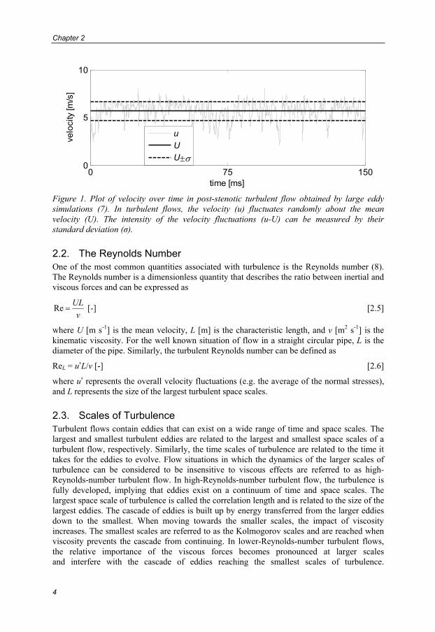
Figure 1. Plot of velocity over time in post-stenotic turbulent flow obtained by large eddy simulations (7). In turbulent flows, the velocity (u) fluctuates randomly about the mean velocity (U). The intensity of the velocity fluctuations (u-U) can be measured by their standard deviation (σ).
2.2. The Reynolds Number One of the most common quantities associated with turbulence is the Reynolds number (8). The Reynolds number is a dimensionless quantity that describes the ratio between inertial and viscous forces and can be expressed as
νUL
=Re [-] [2.5]
where U [m s-1] is the mean velocity, L [m] is the characteristic length, and ν [m2 s-1] is the kinematic viscosity. For the well known situation of flow in a straight circular pipe, L is the diameter of the pipe. Similarly, the turbulent Reynolds number can be defined as
ReL = u’L/ν [-] [2.6]
where u’ represents the overall velocity fluctuations (e.g. the average of the normal stresses), and L represents the size of the largest turbulent space scales.
2.3. Scales of Turbulence Turbulent flows contain eddies that can exist on a wide range of time and space scales. The largest and smallest turbulent eddies are related to the largest and smallest space scales of a turbulent flow, respectively. Similarly, the time scales of turbulence are related to the time it takes for the eddies to evolve. Flow situations in which the dynamics of the larger scales of turbulence can be considered to be insensitive to viscous effects are referred to as high-Reynolds-number turbulent flow. In high-Reynolds-number turbulent flow, the turbulence is fully developed, implying that eddies exist on a continuum of time and space scales. The largest space scale of turbulence is called the correlation length and is related to the size of the largest eddies. The cascade of eddies is built up by energy transferred from the larger eddies down to the smallest. When moving towards the smaller scales, the impact of viscosity increases. The smallest scales are referred to as the Kolmogorov scales and are reached when viscosity prevents the cascade from continuing. In lower-Reynolds-number turbulent flows, the relative importance of the viscous forces becomes pronounced at larger scales and interfere with the cascade of eddies reaching the smallest scales of turbulence.
Disturbed Flow and Turbulence
5
As these flows do not meet the criteria of a fully operable eddy cascade, they are often referred to as transitional or disturbed flows. Following Yellin (9), disturbed flow may be described as a regime of an otherwise laminar flow that contains transient velocity fluctuations. While text books of turbulence deal almost exclusively with the fully developed scenario, fluctuating flows in the human cardiovascular system may often be of the lower-Reynolds-number type. Irrespective of the specific nature of the flow, the standard deviation of the velocity fluctuations is commonly referred to as turbulence intensity and will be so in this thesis as well.
2.4. Experimental Fluid Mechanics of Turbulent Flow For statistical determination of turbulence quantities, ensemble averaging over an infinite number of repeated realizations of the experiment would be desirable (10). As this is not possible in practice, ensemble averaging is replaced by time or space averaging using a finite number of measurements. This is justified by considering turbulence to be ergodic, implying that it is statistically stationary with respect to time and space. In ergodic flows ensemble, time, and space averages of a turbulence quantity have the same value (10, 11). Irrespective of the choice of averaging approach, an important aspect of turbulence measurements is to sample all the scales of turbulence that are present in the region of interest. Conventionally in experimental fluid mechanics of turbulent flow, this is achieved by sampling a small spatial region over time. Established experimental methods that are able to quantify the intensity of velocity fluctuations include thermal anemometry, laser Doppler anemometry (LDA), and particle image velocimetry (PIV) (12-14). The specific challenges associated with measurements of turbulence quantities of each of these methods increase with higher levels of turbulence intensity (10, 15). Thermal anemometry methods, including hot-wire and hot-film anemometry, utilize electronically heated sensors that are exposed to the flowing fluid. The flow velocity is measured by exploiting its relationship to the convective heat transfer from the sensor. Thermal anemometry methods have the potential to achieve temporal resolutions up to 10-2 ms and spatial resolutions of a few micrometers. Thermal anemometry, in contrast to optical methods, can be used to measure turbulence quantities in the central parts of the cardiovascular system; this is an invasive process, however, where the sensor is placed via a catheter. Further introduction to the in vivo assessment of turbulence will follow in chapter 3. Optical methods for experimental fluid dynamics, including LDA and PIV, are based on the interaction of light with a fluid particle suspension. LDA transmits a laser beam through the suspension and exploits the fact that light scattered from the particles in the suspension experiences a frequency (Doppler) shift that is dependent on their speed. The maximum obtainable spatial and temporal resolutions in LDA are an order of magnitude lower than those from thermal anemometry. PIV employs digital image recording of two short-duration planar laser sheets. Velocity is computed based on the spatial displacement of the particles between the exposures. The spatial resolution of PIV is lower than that in LDA, but PIV has the advantage of being a two-dimensional (2D) method.

7
3. Disturbed Blood Flow in the Human
Cardiovascular System
While blood flow in the normal cardiovascular system appears to be remarkably free of turbulence, cardiovascular diseases including valvular and vascular stenoses and valvular insufficiencies can cause disturbed or turbulent blood flow (16-18). A direct consequence of turbulent cardiovascular blood flow is the decrease in blood transport efficiency that is caused by viscous dissipation, which is the major cause of pressure drop over tight stenoses (18). Fluctuations in velocity and pressure impose fluid mechanical forces on its surroundings. Exposure of blood constituents to these abnormal forces has been associated with hemolysis (19-21) as well as platelet activation and aggregation (22, 23). Furthermore, ample evidence supports the long-standing theory that disturbed hemodynamics play an important role in the initiation and progression of atherosclerosis (24-29). In spite of being associated with risk factors with widespread systemic impact such as smoking, hypertension, and elevated levels of cholesterol, atherosclerotic plaques are predominately initiated at branch points, sharp bends, and other regions of the arterial tree where the blood flow is altered. This is well demonstrated by the carotid artery bifurcation which appears to host a unique flow environment and is one of the most common sites for atherosclerotic disease (30). In the advanced stages of atherosclerotic disease, plaque rupture can lead to thrombosis and embolism which can obstruct the blood supply of heart or brain. While the intrinsic vulnerability of the plaque predisposes it to rupture, the rupture itself may be triggered by extrinsic fluid mechanical forces (31). In cardiovascular medicine, a commonly recognized feature of turbulence is the audible sounds that are created by fluctuations in pressure (32). These sounds can be detected by stethoscopes. For several decades, the stethoscope served as the critical tool for the localization and assessment of the severity of several cardiovascular diseases, including mitral regurgitation and aortic valve stenosis. With the advent of diagnostic imaging the role of auscultation has declined. Measurements of turbulence quantities in vivo have only been possible using highly invasive methods and as a result, the number of studies performed in humans is small (18, 33). Using catheter-based thermal anemometry, Stein and Sabbah (16) made measurements of turbulence intensity in seven healthy subjects, seven patients with aortic valve disease and one patient with aortic valve prosthesis. Their findings indicated that the ascending aortic blood flow is turbulent in patients with aortic valve disease and that it is disturbed in normal subjects. In the pulsatile blood flow of humans, turbulence occurs primarily during the decelerating period of the flow waveform because acceleration has a stabilizing effect on flow. This has been documented in studies performed in vitro (34, 35), in animal models (36), as well as in humans (16). An ultrasound approach to the assessment of disturbed and turbulent flows has been presented and utilized by Nygaard et al. (37, 38). They designed a perivascular Doppler ultrasound system permitting bi-directional measurements of turbulence intensity in surgically
Chapter 3
8
exposed aortas and applied this system to document turbulence in patients who underwent aortic valve replacement. Ultrasound has provided different approaches also to the non-invasive assessment of turbulence, including analysis of spectral broadening and computation of the standard deviation of mean velocities recorded from multiple cardiac cycles, which have been proposed and utilized in various settings (39-43). Non-invasive ultrasound techniques can be applied to the heart and arterial tree at those sites where adequate acoustic windows exist and with further development may prove to be valuable for the determination of turbulence quantities in vivo. The restriction of non-invasive ultrasound methods to measuring velocity only in the single direction defined by the transducer probe may be a limiting factor in the assessment of turbulence (44). Magnetic resonance imaging (MRI) is a versatile non-invasive tool for the quantification and characterization of blood flow (45-47). In contrast to the thermal, optical, and sonic methods described in this and the preceding chapter, MRI can be applied anywhere in the human body and the data can be acquired in three-dimensions (3D) and in an arbitrary number of directions. It is well known that the presence of velocity fluctuations affects the MRI signal (48-50) and the possibility of using MRI to quantify turbulence has been the focus of many studies (51-59). In spite of the significant work done, MRI methods for the measurement of turbulence quantities have not reached the status of applicability and no in vivo measurements have been reported.
9
4. Magnetic Resonance Imaging
Sub-atomic particles like electrons and atomic nuclei possess intrinsic magnetism. This implies that they have a spin angular momentum and a magnetic moment, which are proportional to each other via the gyromagnetic ratio. For the hydrogen proton, the gyromagnetic ratio is γ = 2.68x10⁸ rad/s/T. When exposed to an external magnetic field, B0, the magnetic moments, or spins, align with and undergo precession around that field. The rate of angular precession is described by the Larmor equation
ω0 = γ B0 [rad/s] [4.1]
where ω0 denotes the Larmor frequency. Fields strengths of 1.5 T and 3 T are typically used in clinical whole-body MRI scanners, in which case the Larmor frequency is 64 and 128 MHz, respectively. By altering the external magnetic field, the Larmor frequency can be varied; this is utilized to perform MR imaging and velocity measurements, as described in this chapter. Several achievements in the development of MRI have been recognized by the Noble Prize committee. In 1938, Rabi and co-workers (60) introduced the concept of using magnetic resonance to measure the magnetic moment of nuclei. Rabi was awarded the Nobel Prize in Physics in 1944. In 1946, Bloch (61) and Purcell (62) performed the first successful experiments to detect the magnetic resonance phenomenon and were subsequently awarded the Nobel Prize in Physics in 1952. The development of what is known today as MRI gained speed in the 1970’s when the utilization of magnetic field gradients to create images was described by Lauterbur (63, 64) and further developed by Mansfield (65). In 2003, Lauterbur and Mansfield shared the Nobel Prize in Physiology or Medicine.
4.1. Signal Generation By considering a macroscopic packet of spins, rather than considering each spin individually, a classical physics representation can be employed. In this way, the spin packet can be represented by its net magnetization vector M. In the relaxed state, M is aligned with the external magnetic field. The orientation of M can be altered by applying radio-frequency (RF) pulses that match the Larmor frequency. When the RF-pulse is switched off, the magnetization undergoes relaxation and thereby returns to its original alignment with the external magnetic field. The relaxation is described by the Bloch equation
zyxBMM ˆ1T
ˆ2T
ˆ2T
0MMMMγdt
d zyx −−−−×= [4.2]
where T1 and T2 are referred to as the spin-lattice (or longitudinal) and the spin-spin (or transversal) relaxation time, respectively. T1 describes the time it takes for the longitudinal component of M (Mz) to recover 63% of its initial value (M0), and is a result of the return of excited spins to their relaxed state. T2 reflects the time it takes for the transverse component of M (Mxy) to decay to 63% of its original value.

Chapter 4
10
The T2 decay is a result of the interaction between spins which makes them lose their phase coherence. Both T1 and T2 are tissue specific parameters; this can be exploited to distinguish different tissue types. As the magnetization returns to its original alignment with the external magnetic field a time-varying signal is induced in the receiver coil(s). This signal is known as the free-induction decay signal and is the basis for MRI.
4.2. Image Formation For the generation of images, magnetic field gradients are used. A magnetic field gradient vector G causes the magnetic field to vary spatially over the object being imaged and thus the Larmor frequency will depend on the position r according to
ω = γ (B0 + G·r) [4.3]
In this way, spins will accumulate phase according to
∫ ⋅=t
dttγφ0
')'( rG [4.4]
where G(t') describes the time-varying magnetic field gradient waveform and t' = 0 is the time for excitation. The time-varying magnetic field gradients in combination with the timing of the RF excitation are described by the pulse sequence. A 2D gradient-echo pulse sequence is illustrated in Figure 2. The time it takes to execute one cycle of the repetitive pulse sequence is referred to as the repetition time (TR). The time between the application of the RF pulse and the time point at which the echo signal strength reaches its maximum is called the echo time (TE). Signal readout can be made symmetrically or asymmetrically (partial echo) around TE. By the use of a quadrature detector, the signal induced in the receiver coil is split up into a real and an imaginary part. Under the assumption that the T2 relaxation time is much longer than the time for the application of the gradients, the resulting complex demodulated MRI signal is a function of the applied gradient waveform and the object being imaged, f(r), according to the Fourier transform
∫∫Ω
⋅−
Ω
−∫
== rrrrr
r defdeftS
tdtttγi
tφi 0
')'()'(),( )()()(
G
[4.5]
where Ω is the excited volume. The magnetic field gradient vector G(t’) controls the navigation in k-space (66, 67), which is the spatial frequency domain in which the image is being sampled (Figure 2).

Magnetic Resonance Imaging
11
Figure 2. 2D gradient echo pulse sequence (left) and the sampling of one line in k-space (right). A slice encoding gradient encodes a kz position. Prior to the occurrence of the echo signal, phase encoding determines the ky line to be sampled and the initial part of the readout gradient determines at what kx position to start. Sampling a row in k-space is achieved by the remaining portion of the readout gradient. To sample the complete 2D k-space, this scheme is repeated for a number of phase-encoding steps. In a 3D pulse sequence, phase-encoding gradients are added to the slice-encoding direction. The k-space variables can be written as
( ) ∫=t
dttπγt
0
')'(2
Gk [4.6]
In this way, equation 4.5 can be written as
( )( ) ∫Ω
⋅−= rr deftS πi rkk 2)( [4.7]
where S(k) is the k-space data. Taking the inverse Fourier transform gives the complex-valued image domain data. The image domain data can be presented in different ways. The most common way is to display a magnitude image, which is obtained by taking the modulus of the complex data (Figure 3).
Figure 3. The data acquired in MRI are stored in the k-space (a). The Fourier transform of the k-space gives the image domain data. Each voxel in the image can be represented by a complex-valued number (b). Most commonly the MRI data is shown as magnitude image (c). Another option is to display a phase image (d).
kx
ky
RF t´
Greadout
t´
Gslice
t´
Signal t´
Gphase
t´
Imag
Real φ
(a) (b) (c) (d)
Chapter 4
12
Different strategies for playing out the gradients G(t’) to traverse the k-space exist, each associated with specific advantages and limitations. The most basic way of collecting the k-space data is by Cartesian traversal in a row-by-row manner. This can be achieved using the pulse sequence described in Figure 2. The spatial coverage in image space is referred to as the field-of-view (FOV). In a dimension (x) of the image FOVx = xmax - xmin = 1/Δkx, where Δkx represent the spacing between two adjacent samples in the k-space. The spatial resolution in the image, δ, is inversely proportional to the size of the k-space according to δx = 1/(kx,max – kx,min). In this way, the minimum number of samples necessary to achieve a specific field-of-view and spatial resolution is Nx = FOVx/δx= (kx,max – kx,min)/Δkx. In 2D imaging, the spatial resolution is commonly referred to in terms of pixel size and slice thickness. In the case of 3D imaging, the spatial resolution is the size of an image volume element, or voxel.
4.3. Cardiac Gating By acquiring the k-space data at several instances of the cardiac cycle, time-resolved images can be obtained. This can be achieved by synchronizing the data acquisition to the cardiac cycle using electrocardiogram or photoplethysmograph controlled gating. Different methods to achieve cardiac gating exist. Prospective cardiac gating (68) utilizes a predefined acquisition time window and may thus be used when only a fraction of the cardiac cycle is of interest. In contrast to prospective gating, retrospective gating (69), often referred to as cine imaging, permits the acquisition of a complete cardiac cycle. This can be achieved by simultaneous data acquisition and monitoring of the electrocardiogram. Because of heart rate variations, the number of acquired time frames may differ between different heart beats. Therefore, a temporal sliding-window approach is usually employed to reconstruct the acquired data into a set of evenly distributed time frames. Using gating in the most basic configuration, one k-space line is acquired per cardiac cycle. Alternatively, a number of k-space lines can be acquired per cardiac cycle; this enables a tradeoff between scan time and temporal resolution and is commonly described as a segmented k-space acquisition. The number of steps in the temporal domain of the resulting k-t space corresponds to the number of acquired time frames, and the temporal separation between each step determines the temporal resolution.

Magnetic Resonance Imaging
13
4.4. MRI Flow Imaging Spins with constant velocity that move parallel to a magnetic field gradient will acquire a phase shift proportional to their velocity; therefore, MRI has an inherent sensitivity to motion. Including motion terms up to the first order, the spin position vector r can be written as
r(t) = r0+ut [4.8]
Inserting into the phase accumulation function (equation 4.4) gives
[ ] 1000
0 ')'(),( MuMur ⋅+⋅=∫ +⋅= γγdtttγtφt
rGr [4.9]
where M0 and M1 are the 0th and 1st moments of the applied gradient waveform. M1 determines the sensitivity of the gradient waveform to first order motion. In MRI applications where specific motion sensitivity is wanted, the motion sensitivity in the pulse sequence is typically controlled by adding bipolar gradients (Figure 4), and the other gradients are configured so as to produce a zero net M1 (gradient moment nulling). In analogy with the k-space description of spatial encoding, velocity-encoding can be expressed in terms of a velocity kv-space where
kv = γM1 [4.10]
may be referred to as the velocity frequency encoding. In the ideal case, kv defines a proportionality between the phase-shift of a spin packet and its velocity. However, due to factors other than spin motion, such as magnetic field inhomogeneities, an additional phase-shift, φadd, is introduced. Adding φadd and the kv-dimensions, the complex-valued MRI signal can be written as
( ) ∫ ∫ ⎟⎟⎠
⎞⎜⎜⎝
⎛= ⋅−+⋅−
R V
iφiπi ddesefS ruurkk ukrk vv )()(, add2
[4.11]
where s(u) represents the distribution of spin velocities that are present in a voxel. R and V indicate integral over space and velocity, respectively. Taking the inverse Fourier transform with respect to the spatial variables gives
( ) ∫ ⋅−=V
iφi desefS uurk ukvv )()( add [4.12]
Figure 4. An ideal bipolar gradient.
t´0 τ 2τ
+G
-G
Chapter 4
14
4.4.1. Phase-Contrast MRI Velocity Mapping The most common MRI technique for the measurement of fluid flow velocity is phase-contrast MRI (PC-MRI) velocity mapping (70, 71). Other names used in the literature to describe this technique include velocity-encoded, flow-sensitive, phase-difference, and phase-mapping MRI. PC-MRI velocity mapping may be viewed as a special case of Fourier velocity encoding (FVE) (72, 73), which will be described in the next section. If the intravoxel spin velocity distribution s(u) is symmetric about the mean velocity U, the argument of the complex-valued MRI signal S(kv) in equation 4.12, its phase-shift, is related to the mean velocity according to
addφφ +⋅= Ukv [4.13]
The effects of intravoxel spin velocity distributions that are not symmetric about the mean velocity have been described by Hamilton et al. (74), among others, and will be explored further in chapter 6. As the additional phase-shift φadd is independent of kv, it can be eliminated by subtracting the phase-shifts of two sets of data, or flow-encoding segments, acquired with different 1st gradient moments:
Ukv ⋅Δ=Δφ [4.14]
where Δkv is proportional to the net 1st gradient moment of two flow-encoding segments. In this way, the mean velocity, U, of the spins within a voxel can be obtained by exploiting that
vφ kU ΔΔ= / [4.15]
which is done in PC-MRI velocity mapping. The two most common approaches to achieving a flow-encoding of Δkv may be referred to as symmetric and asymmetric. Symmetric implies that the two segments needed for one-directional flow-encoding are acquired with +½kv and -½kv, respectively. In asymmetric flow-encoding, the same Δkv is obtained by acquiring one segment with a zero 1st gradient moment and the other with a flow-sensitivity of kv. A critical parameter in PC-MRI velocity mapping is the velocity encoding range (VENC), which is defined as the velocity that gives a phase shift of π radians. The VENC is related to Δkv according to
vπ kΔ= /VENC [4.16]
If the true velocity is outside the ±VENC range, the measured velocity estimate aliases back into that range and can thus not be unambiguously determined. Although velocity aliasing can be corrected for to some extent (75), this is something that is usually avoided by appropriate tuning of the VENC parameter. Consequently, when carrying out a PC-MRI velocity mapping measurement it is valuable to have an estimate of the highest expected velocity in the region of interest. To create time-resolved velocity images that cover a complete cardiac cycle, PC-MRI is typically combined with cine imaging (76, 77). The two flow-encoding segments needed for a one-directional velocity measurement are often acquired in an interleaved manner, implying that data for both segments are acquired during each cardiac cycle. Interleaved flow-encoding reduces artifacts due to subject motion at the cost of temporal resolution.
Magnetic Resonance Imaging
15
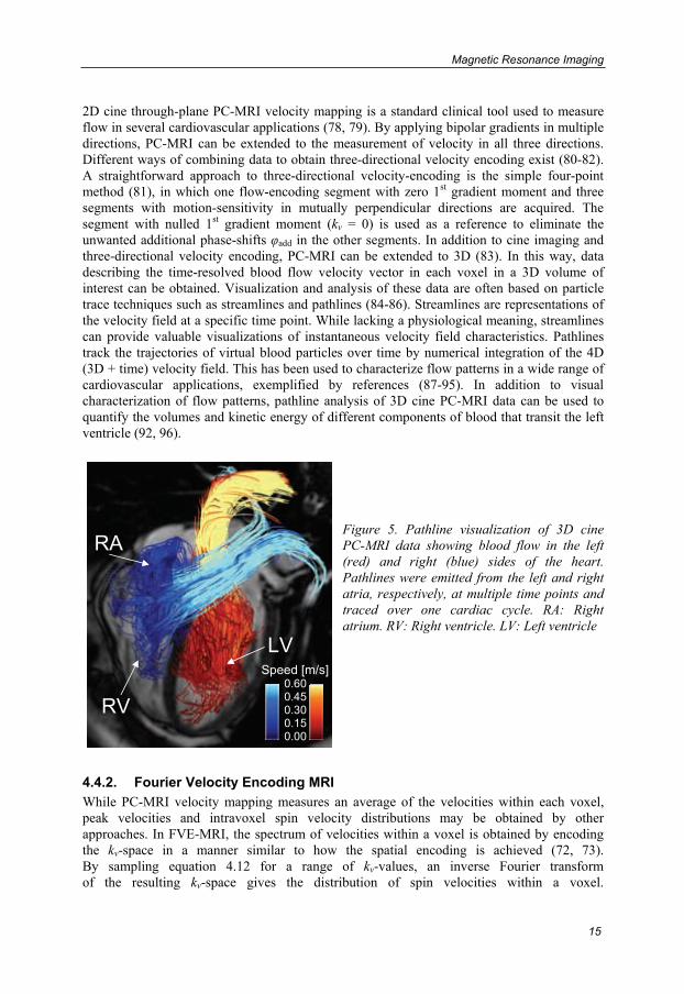
2D cine through-plane PC-MRI velocity mapping is a standard clinical tool used to measure flow in several cardiovascular applications (78, 79). By applying bipolar gradients in multiple directions, PC-MRI can be extended to the measurement of velocity in all three directions. Different ways of combining data to obtain three-directional velocity encoding exist (80-82). A straightforward approach to three-directional velocity-encoding is the simple four-point method (81), in which one flow-encoding segment with zero 1st gradient moment and three segments with motion-sensitivity in mutually perpendicular directions are acquired. The segment with nulled 1st gradient moment (kv = 0) is used as a reference to eliminate the unwanted additional phase-shifts φadd in the other segments. In addition to cine imaging and three-directional velocity encoding, PC-MRI can be extended to 3D (83). In this way, data describing the time-resolved blood flow velocity vector in each voxel in a 3D volume of interest can be obtained. Visualization and analysis of these data are often based on particle trace techniques such as streamlines and pathlines (84-86). Streamlines are representations of the velocity field at a specific time point. While lacking a physiological meaning, streamlines can provide valuable visualizations of instantaneous velocity field characteristics. Pathlines track the trajectories of virtual blood particles over time by numerical integration of the 4D (3D + time) velocity field. This has been used to characterize flow patterns in a wide range of cardiovascular applications, exemplified by references (87-95). In addition to visual characterization of flow patterns, pathline analysis of 3D cine PC-MRI data can be used to quantify the volumes and kinetic energy of different components of blood that transit the left ventricle (92, 96).
Figure 5. Pathline visualization of 3D cine PC-MRI data showing blood flow in the left (red) and right (blue) sides of the heart. Pathlines were emitted from the left and right atria, respectively, at multiple time points and traced over one cardiac cycle. RA: Right atrium. RV: Right ventricle. LV: Left ventricle
4.4.2. Fourier Velocity Encoding MRI While PC-MRI velocity mapping measures an average of the velocities within each voxel, peak velocities and intravoxel spin velocity distributions may be obtained by other approaches. In FVE-MRI, the spectrum of velocities within a voxel is obtained by encoding the kv-space in a manner similar to how the spatial encoding is achieved (72, 73). By sampling equation 4.12 for a range of kv-values, an inverse Fourier transform of the resulting kv-space gives the distribution of spin velocities within a voxel.
LV
RV
RA
0.600.450.300.150.00
Speed [m/s]
Chapter 4
16
In analogy with the definitions of spatial field-of-view and resolution (section 4.2), the velocity field-of-view and the velocity resolution are defined as FOVv = 1/Δkv and δv = 1/(kv,max – kv,min), respectively. Consequently, the number of flow-encoding segments necessary to achieve a specific velocity field-of-view and resolution in FVE is N = FOVv/δv= (kv,max – kv,min)/Δkv. As a complete spatiotemporal k-t space is acquired for each value of kv, many potential applications of FVE are not feasible due to the inherently long scan time. Depending on the specific application, different tradeoffs can be used to reduce the imaging time (97-102). Examples of applications where FVE have demonstrated feasibility include the quantification of peak velocities in flow jets (103, 104) and the determination of wall shear rate, which is the velocity gradient at the vessel wall (105, 106). A useful FVE approach for the quantification of turbulence intensity has not yet been reported.
4.5. Effects of Velocity Fluctuations on the MRI Signal The presence of velocity fluctuations, as in disturbed and turbulent flows, decreases the MRI signal magnitude under the influence of a magnetic field gradient (48-50, 107, 108). Mechanisms involved in the reduction of the signal magnitude due to velocity fluctuations include ghosting and intravoxel phase dispersion. Ghosting is caused by variations in the mean signal phase and amplitude between readouts and results in displacement of the signal contributions from their correct position. Because of the random nature of velocity fluctuations, the displaced signal appears as blurry streaks in the image. Intravoxel phase dispersion is caused by the presence of a distribution of spin velocities within a voxel, which gives rise to destructive interference of signal phases. Of the mechanisms involved in creating signal loss due to velocity fluctuations, intravoxel phase dispersion has been shown to be the largest determinant (49, 109). Similar to intravoxel phase dispersion due to velocity fluctuations, spatial mean velocity gradients also give rise to a distribution of velocities within a voxel and can thereby also cause signal loss. The relative impact of signal loss caused by mean velocity variations has been reported to be small if compared to signal loss caused by velocity fluctuations (109). Many clinical applications depend on accurate PC-MRI mean velocity measurements in flow fields that may be turbulent, for example downstream from a stenosis. A decrease in MRI signal amplitude leads to an increased uncertainty in the mean velocity estimates, so minimizing signal loss is important in preserving the accuracy of PC-MRI velocity mapping (107, 110, 111). A frequently mentioned approach to decreasing signal loss is to reduce TE. However, the diminished signal loss that has been observed in studies evaluating the effect of reduced TE are more likely the result of concomitant modifications in the gradient waveform, rather than the shorter TE itself (49, 107). While minimization of signal loss is of paramount importance in many applications, another research direction has focused on relating the signal loss to hemodynamic parameters. For example, it has been suggested that the degree and amount of signal loss in itself could be used for hemodynamic grading of vascular stenosis (112) and valvular stenosis and regurgitation (113). However, the utility of semi-quantitative approaches for hemodynamic evaluation that are based on signal loss alone is limited because variation in imaging parameters will greatly affect the extent and degree of the signal loss (114).
Magnetic Resonance Imaging
17
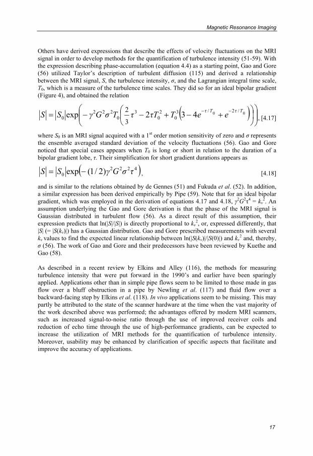
Others have derived expressions that describe the effects of velocity fluctuations on the MRI signal in order to develop methods for the quantification of turbulence intensity (51-59). With the expression describing phase-accumulation (equation 4.4) as a starting point, Gao and Gore (56) utilized Taylor’s description of turbulent diffusion (115) and derived a relationship between the MRI signal, S, the turbulence intensity, σ, and the Lagrangian integral time scale, T0, which is a measure of the turbulence time scales. They did so for an ideal bipolar gradient (Figure 4), and obtained the relation
( ) ⎟⎟⎠
⎞⎜⎜⎝
⎛⎟⎠⎞
⎜⎝⎛ +−+−−= −− 00 /2/3
02
03
0222
0 432exp3
2 TτTτ eeTTττTσGγSS , [4.17]
where S0 is an MRI signal acquired with a 1st order motion sensitivity of zero and σ represents the ensemble averaged standard deviation of the velocity fluctuations (56). Gao and Gore noticed that special cases appears when T0 is long or short in relation to the duration of a bipolar gradient lobe, τ. Their simplification for short gradient durations appears as
( )42220 )2/1(exp τσGγSS −= , [4.18]
and is similar to the relations obtained by de Gennes (51) and Fukuda et al. (52). In addition, a similar expression has been derived empirically by Pipe (59). Note that for an ideal bipolar gradient, which was employed in the derivation of equations 4.17 and 4.18, γ2G2τ4 = kv
2. An assumption underlying the Gao and Gore derivation is that the phase of the MRI signal is Gaussian distributed in turbulent flow (56). As a direct result of this assumption, their expression predicts that ln(|S|/|S|) is directly proportional to kv
2, or, expressed differently, that |S| (= |S(kv)|) has a Gaussian distribution. Gao and Gore prescribed measurements with several kv values to find the expected linear relationship between ln(|S(kv)|/|S(0)|) and kv
2 and, thereby, σ (56). The work of Gao and Gore and their predecessors have been reviewed by Kuethe and Gao (58). As described in a recent review by Elkins and Alley (116), the methods for measuring turbulence intensity that were put forward in the 1990’s and earlier have been sparingly applied. Applications other than in simple pipe flows seem to be limited to those made in gas flow over a bluff obstruction in a pipe by Newling et al. (117) and fluid flow over a backward-facing step by Elkins et al. (118). In vivo applications seem to be missing. This may partly be attributed to the state of the scanner hardware at the time when the vast majority of the work described above was performed; the advantages offered by modern MRI scanners, such as increased signal-to-noise ratio through the use of improved receiver coils and reduction of echo time through the use of high-performance gradients, can be expected to increase the utilization of MRI methods for the quantification of turbulence intensity. Moreover, usability may be enhanced by clarification of specific aspects that facilitate and improve the accuracy of applications.


19
5. Aims
The aim of this thesis was to develop an MRI method that permits non-invasive quantification of turbulence intensity in the pulsatile blood flow of humans. The specific sub aims were to:
• Develop a framework for the quantification of turbulence intensity using MRI. • Validate the derived method by in vitro comparison with established approaches for
experimental fluid mechanics. • Extend the method to the in vivo determination of turbulence intensity. • Address fluid mechanical aspects of cardiovascular disease using the method.

21
6. Generalized MRI Framework for the
Quantification of any Moment of Arbitrary
Velocity Distributions
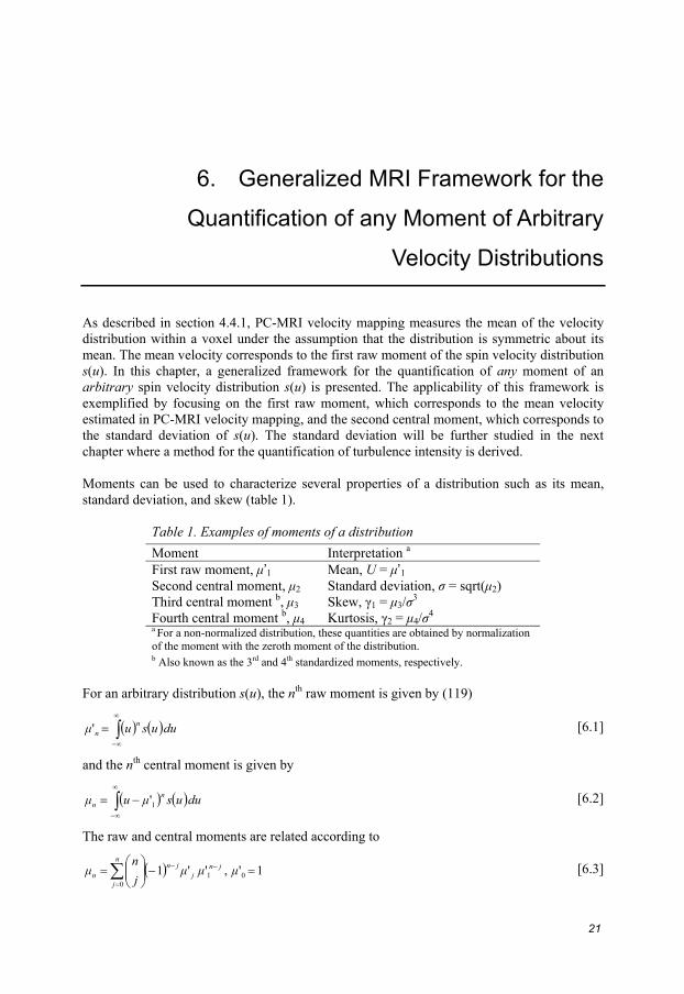
As described in section 4.4.1, PC-MRI velocity mapping measures the mean of the velocity distribution within a voxel under the assumption that the distribution is symmetric about its mean. The mean velocity corresponds to the first raw moment of the spin velocity distribution s(u). In this chapter, a generalized framework for the quantification of any moment of an arbitrary spin velocity distribution s(u) is presented. The applicability of this framework is exemplified by focusing on the first raw moment, which corresponds to the mean velocity estimated in PC-MRI velocity mapping, and the second central moment, which corresponds to the standard deviation of s(u). The standard deviation will be further studied in the next chapter where a method for the quantification of turbulence intensity is derived. Moments can be used to characterize several properties of a distribution such as its mean, standard deviation, and skew (table 1).
Table 1. Examples of moments of a distribution Moment Interpretation a First raw moment, μ’1 Mean, U = μ’1 Second central moment, μ2 Standard deviation, σ = sqrt(μ2) Third central moment b, μ3 Skew, γ1 = μ3/σ3 Fourth central moment b, μ4 Kurtosis, γ2 = μ4/σ4 a For a non-normalized distribution, these quantities are obtained by normalization of the moment with the zeroth moment of the distribution. b Also known as the 3rd and 4th standardized moments, respectively.
For an arbitrary distribution s(u), the nth raw moment is given by (119)
( ) ( )duusuμ nn ∫
∞
∞−
=' [6.1]
and the nth central moment is given by
( ) ( )duusμuμ nn ∫
∞
∞−
−= 1' [6.2]
The raw and central moments are related according to
( ) 1',''1 010
=−⎟⎟⎠
⎞⎜⎜⎝
⎛= −
=
−∑ μμμjn
μ jnj
n
j
jnn [6.3]

Chapter 6
22
Moment in the function domain (velocity-space) corresponds to derivation in the transform domain (kv-space) at kv = 0 (120). The raw moments of the intravoxel velocity distribution s(u) are related to the MRI signal S(kv) according to
( ) ( ) 0=
∞
∞−
=∫ vkvnv
nnn kS
dkdiduusu [6.4]
Thus, to obtain the nth moment of arbitrary intravoxel spin velocity distributions, the nth derivative of the MRI signal S(kv) with respect to kv at kv = 0 needs to be determined.
6.1. Mean Velocity of a Voxel As described in section 4.4.1, PC-MRI velocity mapping estimates the mean velocity under the assumption that s(u) is symmetric about its mean. To obtain the mean velocity without this or any other assumptions, the first derivative of S(kv) at kv = 0 needs to be determined. Letting T(kv) = S(kv)/S(0), where S(0) corresponds to the zeroth moment of s(u), represent a normalized MRI signal, PC-MRI velocity mapping can be derived from the moment theory described above. As s(u) is real, S(kv), and thereby also the normalized distribution T(kv), is Hermitian. The real part of an Hermitian function, x(kv) = real(T(kv)), is an even function and the imaginary part, y(kv) = imag(T(kv)), is an odd function. By exploiting that the limit of dx(kv)/dkv as kv approaches zero is zero it can be seen that the first derivative of T(kv)
( )0, →→+= v
vvvv
v kdkdyi
dkdyi
dkdx
dkkdT [6.5]
Thus, for small values of kv, the first raw moment it related to the imaginary part of the MRI signal according to
( )vv
v
dkdy
dkkdT
iμ −==1' [6.6]
By also exploiting that the limits of y(kv) and x(kv) as kv approaches zero is zero and one, respectively, it can be seen that the first derivative of the argument of T(kv)
( )( )( )
0,/1
1arctanarg 22 →→−
+=⎥
⎦
⎤⎢⎣
⎡⎟⎠⎞
⎜⎝⎛= v
v
vv
vv
v
kdkdy
xdkdxy
dkdyx
xyxy
dkdkT
dkd [6.7]
Thus, for small values of kv, the derivative of arg(T(kv)) is equal to the derivative of the imaginary part of the MRI signal. If the velocity u is represented by u = U + udev, where U is the mean velocity of a voxel and udev is the deviation of each spin’s velocity from the mean velocity of the voxel, as done by Hamilton et al. (74), it is found that
( )
⎟⎟⎠
⎞⎜⎜⎝
⎛++−=
=⎟⎟⎠
⎞⎜⎜⎝
⎛+=
⎟⎟⎠
⎞⎜⎜⎝
⎛=
∫
∫
∫
∞
∞−
−
∞
∞−
−−
∞
∞−
−
devdev
devdev
dev
dev
)(arg
)(arg
)(arg)(arg
dueuUsUk
dueuUse
dueuskT
uikv
uikUik
uikv
v
vv
v
[6.8]

Generalized MRI Framework for the Quantification of any Moment of Arbitrary Velocity Distributions
23
As a real symmetric function has a real Fourier transform, the last term in equation 6.8 will be zero if the distribution is symmetric. Thus, if s(u) is symmetric about its mean, arg(T(kv)) is linear on the interval |kv| < π / U and its derivative at kv = 0 can be obtained from measurements made with larger values of kv. This, in combination with the relationship between the first derivatives of T(kv) and arg(T(kv)) at kv = 0 (equations 6.5-6.7), leads to the following approach for the estimation of the mean velocity U (the first raw moment of s(u)) that does not require measurements solely at kv ~ 0:
( )( ) ( )( ) ( )( )v
v
v
v
kkSS
kkT
Uarg0argarg −
=−= , |kv| < π / U [6.9]
or, more generally,
( )( ) ( )( )v
vv
kkSkS
UΔ
−= 12
argarg, |∆kv| < π / U [6.10]
which corresponds to equation 4.15 used in PC-MRI velocity mapping (section 4.4.1).
6.2. Standard Deviation of the Intravoxel Velocity Distribution The standard deviation of s(u) (intravoxel velocity standard deviation (IVSD)) corresponds to the square-root of the second central moment of s(u), μ2, which is related to the first and second raw moments according to
2122 '' μμμ −= [6.11]
μ’2 is the root-mean-square (RMS) of the velocity. Letting ( ) ( ) ( )0/ SkSkT vv = , μ’2 can for small kv be estimated by a finite difference approximation:
( ) ( ) ( )202
2
22'
v
vvk
v
v
kkTkT
dkkTdμ
v
−+−−≈−= = [6.12]
Writing T(kv) in polar form and using Euler’s formula, the rightmost term in equation 6.12 can be written as
( ) ( ) ( ) ( )( )22
cos222
v
vv
v
vv
kkθkT
kkTkT −
=−+−
− [6.13]
where θ is the argument of T(kv) and related to μ’1 according to the previous section. A Taylor series expansion of ( )( )vkθcos around kv = 0 gives
( ) ( )( ) ( )( ) ( ) ( ) ( )22
22
12cos22v
v
vv
v
v
v
vv kΟdk
kθdkTk
kTk
kθkT+⎟⎟
⎠
⎞⎜⎜⎝
⎛+
−=
− [6.14]
A Taylor expansion of |T(kv)| in the second term on the right hand side of equation 6.14 around kv = 0 gives ( ) ( )21 vv kΟkT += and thus for small kv:
( ) ( )( ) 2122 '
0/12' μ
kSkS
μv
v +−
= [6.15]
where the relationship between θ and μ’1 derived in the previous section has been exploited.
Chapter 6
24
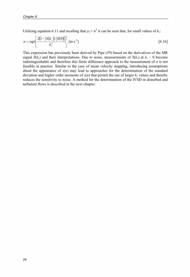
Utilizing equation 6.11 and recalling that μ2 = σ
2 it can be seen that, for small values of kv:
( ) ( )( )⎥⎦
⎤⎢⎣
⎡ −= 2
0/12sqrt
v
v
kSkS
σ [m s-1] [6.16]
This expression has previously been derived by Pipe (59) based on the derivatives of the MR signal S(kv) and their interpretations. Due to noise, measurements of S(kv) at kv ~ 0 become indistinguishable and therefore this finite difference approach to the measurement of σ is not feasible in practice. Similar to the case of mean velocity mapping, introducing assumptions about the appearance of s(u) may lead to approaches for the determination of the standard deviation and higher order moments of s(u) that permit the use of larger kv values and thereby reduces the sensitivity to noise. A method for the determination of the IVSD in disturbed and turbulent flows is described in the next chapter.

25
7. Quantification of Turbulence Intensity using
MRI: Theory and Validation
(Papers I and II) In this chapter, a method for the quantification of the intensity of velocity fluctuations in disturbed or turbulent flows is described. A derivation of this method is presented in section 7.1, followed by in vitro validation in section 7.2. In sections 7.3 and 7.4, potential pitfalls and sources of error in MRI quantification of turbulence intensity, along with approaches for minimizing their effects, are investigated.
7.1. Derivation and Interpretation As described in section 2.4, for statistically stationary (ergodic) flows, turbulence quantities can be measured by using temporal and/or spatial sampling, given that the sampling is made in a way that adequately encompasses the turbulence scales. When these conditions are satisfied, the IVSD would correspond to a measurement of the turbulence intensity, σ, as done by optical and thermal anemometry methods. As described in chapter 6, the IVSD corresponds to the square root of the second central moment of s(u), and to measure this moment without making assumptions about the appearance of s(u) the second derivative of the MRI signal S(kv) at kv = 0 is required. This is difficult in practice because of noise. Therefore, as done in PC-MRI velocity mapping, it may be convenient to introduce an assumption about the appearance of s(u). The probability density functions of turbulent velocity fluctuations are often found to be close to Gaussian, whereas those of derivatives of the velocity fluctuations are not (6, 121). Support for why the velocity distribution is often found to be close to Gaussian may be obtained from the central limit theorem which states that for a set of N independent random variables [X1, X2, …, Xn] where each Xi have an arbitrary probability distribution, the joint probability distribution approaches a Gaussian distribution as the number of samples increases. Approximating s(u) to be Gaussian distributed thus seems like a reasonable model for disturbed and turbulent flows. Assumptions of Gaussian behavior of velocity fluctuations has previously been employed by several investigators studying the effect of turbulence on the MRI signal (51, 56, 122). Employing the Gaussian model, s(u) can be expressed as the Gaussian probability density function
( )22
'2
1
21)(
Uuσe
πσus
−−
= [7.1]
where σ, the standard deviation of s(u), is the turbulence intensity.
Chapter 7
26
Inserting equation 7.1 into equation 4.12 gives
vv
addiUk
kσφi
v eCekS−−−= 2
22
)( [7.2]
where the scaling factor C, influenced by relaxation parameters, spin density and receiver gain, has been introduced. By combining the expressions of two flow-encoding segments acquired with different 1st gradient moments, S(kv1) and S(kv2), the scaling factor C and the additional phase term can be eliminated:
)(2
)(21
21222
21)()( vv
vv kkiUkkσ
vv ekSkS−−
−−
= [7.3]
Taking the absolute value and rearranging gives
( ) ( )( )⎥⎥
⎦
⎤
⎢⎢
⎣
⎡
−= 22
21
12/ln2
sqrtvv
vv
kk
kSkSσ ,
21 vv kk ≠ [7.4]
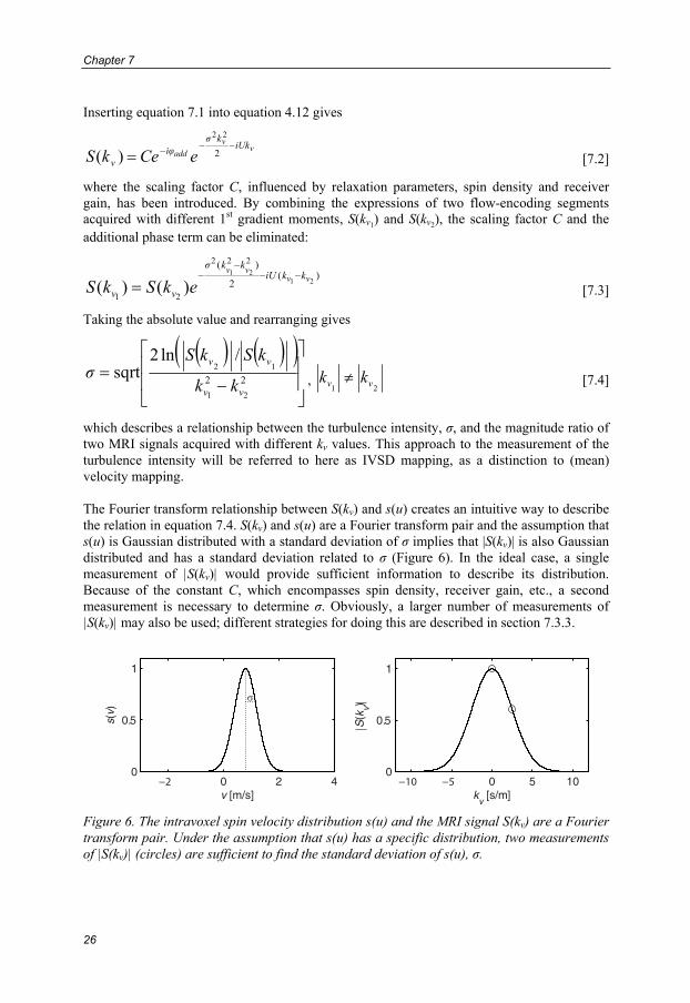
which describes a relationship between the turbulence intensity, σ, and the magnitude ratio of two MRI signals acquired with different kv values. This approach to the measurement of the turbulence intensity will be referred to here as IVSD mapping, as a distinction to (mean) velocity mapping. The Fourier transform relationship between S(kv) and s(u) creates an intuitive way to describe the relation in equation 7.4. S(kv) and s(u) are a Fourier transform pair and the assumption that s(u) is Gaussian distributed with a standard deviation of σ implies that |S(kv)| is also Gaussian distributed and has a standard deviation related to σ (Figure 6). In the ideal case, a single measurement of |S(kv)| would provide sufficient information to describe its distribution. Because of the constant C, which encompasses spin density, receiver gain, etc., a second measurement is necessary to determine σ. Obviously, a larger number of measurements of |S(kv)| may also be used; different strategies for doing this are described in section 7.3.3.
0 2 40
0.5
1
s(v)
v [m/s]0 5 10
0
0.5
1
S(k
v)
kv [s/m]
Figure 6. The intravoxel spin velocity distribution s(u) and the MRI signal S(kv) are a Fourier transform pair. Under the assumption that s(u) has a specific distribution, two measurements of |S(kv)| (circles) are sufficient to find the standard deviation of s(u), σ.

Quantification of Turbulence Intensity using MRI: Theory and Validation
27
IVSD mapping may be described as a velocity-analogue to diffusion-weighted MRI, where the diffusion constant D is obtained from the expression S(b) = S(0)e-bD, where b is a factor depending on the magnetic field gradients and their timing (123). Two or more b values are used to obtain the diffusion. In the derivation of this expression, diffusion is considered to be homogeneous and unrestricted, and thereby Gaussian. In spite of the similarities, diffusion effects are negligible in IVSD measurements of turbulence intensity because the gradient strengths and durations used in IVSD measurements result in b values much smaller than those used in diffusion measurements. IVSD mapping may also be viewed as a model-based approach to FVE. In FVE, described in section 4.4.2, a range of kv values are used to sample S(kv) so that s(u) can be obtained by inverse Fourier transformation. With the assumption that s(u) has a specific distribution, the distribution of its Fourier transform S(kv) is known. If one of the measurements of S(kv) is taken at kv = 0, equation 7.4 can be written as
( )⎥⎦
⎤⎢⎣
⎡= 2
)(/)0(ln2sqrt
v
v
kkSS
σ [7.5]
which corresponds to Gao and Gore’s expression for the case when the bipolar gradient duration, τ, is short if compared to the eddy evolution time, T0 (equation 4.18) (56). This similarity reflects the fact that as the derivation of IVSD mapping utilizes equation 4.12, which encompasses motion terms up to the first order, it is assumed that τ << T0. Experimental methods for the determination of T0 have been described but would have limited applicability in vivo (57, 124). However, as suggested by Gao and Gore (56), T0 can be estimated by l / σ, where l, the characteristic length, is approximated to be one third of the vessel diameter. Based on measurements made in vivo (to be presented in chapter 8), T0 down to 10 ms is a representative minimum estimate for human cardiovascular applications. Consequently, as the duration of a bipolar gradient lobe is around 0.5 ms on modern clinical MRI scanners, the short time-scale assumption, τ << T0, seems to be valid and preferable. As described in section 6.2, equation 6.16, which would permit determination of σ in absence of noise, has also been derived by Pipe (59). To mitigate the noise-sensitivity, Pipe made an empirical adjustment to his derivation which resulted in equation 7.5 and showed that these equations produce the same results for small values of kv.
7.1.1. Generalized PC-MRI If one of the measurements of S(kv) is taken at kv = 0, the data needed to obtain σ can be acquired with an asymmetrically encoded PC-MRI pulse sequence, which is available on many clinical MRI scanners. In this case, the non-zero kv is related to the VENC parameter used in PC-MRI velocity mapping according to kv = π / VENC. Note that this generalized usage of the complex-valued PC-MRI signal permits the estimation of both the turbulence intensity, from the signal magnitude, and the mean velocity, from the signal phase, based on data acquired with a standard PC-MRI pulse sequence. Similar to three-directional velocity-encoding in PC-MRI velocity mapping, the simple four-point method enables three-directional IVSD-encoding. As described in section 2.1, the turbulence intensity, σ, in three mutually perpendicular directions permits the computation of the TKE (equation 2.4), which is a direction independent measure of turbulence intensity.
Chapter 7
28
In PC-MRI velocity mapping, the VENC parameter defines a strict dynamic range. As phase wraps have no effect on the signal magnitude, the dynamic range of IVSD mapping in not in the same way dictated by the VENC. Instead, the VENC defines the point of maximum IVSD sensitivity, σ~ :
σ~ = 1 / kv = π / VENC [7.6]
When the optimal VENCs (kv) for mean velocity and IVSD estimation are not too different, these quantities can be reconstructed from the same data set. The dynamic range of IVSD mapping will be further investigated in section 7.3.
7.1.2. Sampling the Scales of Turbulence In disturbed flows, accurate measurements of the intensity of the velocity fluctuations, σ, as well as the mean velocity U, require sufficient sampling of the turbulence scales (10). Conventional experimental fluid dynamics methods, such as LDA and thermal anemometry, estimate the intensity of velocity fluctuations by taking the standard deviation of repeated velocity measurements in a small spatial region (point). Using these methods a large number of measurements are needed to ensure sufficient sampling of the turbulence (time) scales. The MRI signal is built up by all spins within a voxel, which has a specific spatial extent and is sampled at several points in time during the buildup of the k-space. The spatial sampling of the turbulence scales is simply determined by the spatial extent of the voxel, which captures all space scales smaller than the voxel size. The size of the largest turbulence space scales can be larger that the spatial extent of the voxels, implying that temporal sampling may be necessary to sufficiently capture the largest turbulence scales. How well the temporal dimension assists in sampling the turbulence scales is dependent on the time separation between each sample. When the flow-encoding is fast compared to the evolution of the turbulence scales, so that τ << T0, eddies appear stationary over the short duration of the bipolar gradient. The Lagrangian integral time scale T0 is an order of magnitude representation of the statistical memory of the flow. With this in mind, it may be preferable to keep the consecutive samples temporally separated by more than T0. As stated before, the minimum T0 in human cardiovascular applications is expected to be around 10 ms. For in vivo applications where cardiac gating is used, two consecutive samples (k-space lines) will be temporally separated by the duration of one cardiac cycle and this is not an issue. If a multiple number of phase-encoding lines are acquired per cardiac cycle, an interleaved flow-encoding scheme will keep the consecutive samples separated by at least two TRs for one-directional measurements and four TRs for three-directional measurements, which is about the same order of magnitude as the minimum T0 expected for human cardiovascular applications. In terms of contributions from the temporal domain to the sampling of the turbulence scales, beneficial effects would be expected from signal averaging of multiple acquisitions, given that there is a sufficient temporal separation between the repeated acquisitions of a given phase-encoding line. Increasing the sampling density of the k-space in the phase and slice encoding directions may provide similar effects. The necessity to perform adequate sampling of the turbulence scales applies not only to measurements of turbulence intensity, but also to PC-MRI and FVE approaches for the measurement of mean and peak velocities. As described briefly in section 4.5, variations of the flow field between the acquisitions of the individual phase-encoding lines of a complete k-space cause displacement of the acquired signal in the phase- and slice-encoding directions of the image volume, referred to as ghosting artifacts. Thus, while these variations may be beneficial for the sampling of the turbulence scales, they also induce errors in the estimates. An approach to estimate the combined effect

Quantification of Turbulence Intensity using MRI: Theory and Validation
29
of ghosting and other SNR issues on the accuracy of MRI turbulence measurements has been proposed by Elkins et al. (118). The extent of signal that is displaced from its correct position depends on the encoding strength and therefore, as |kv1| ≠ |kv2|, ghosting can also cause overestimation of the turbulence intensity. As many voxels in a vessel displace signal to each other, it is difficult to quantitatively assess the severity of this artifact for general cases.
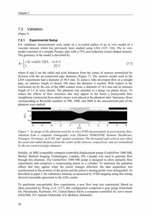
Chapter 7
30
7.2. Validation (Paper I)
7.2.1. Experimental Setup For validation, measurements were made on a re-scaled replica of an in vitro model of a vascular stenosis which has previously been studied using LDA (125, 126). The in vitro model consisted of a straight Perspex pipe with a 75% area-reduction cosine-shaped stenosis. The geometry of the model is described by
( )( )⎪⎩
⎪⎨⎧ <<−+−
>=
22,4/2/cos112,1
ZπZZ
R [7.7]
where R and Z are the radial and axial distances from the center of stenosis normalized by division with the un-constricted pipe diameter (Figure 7). The stenosis model used in the LDA experiments had a diameter of 50.4 mm. To achieve fully developed flow in a straight pipe, an entrance length of almost 100 times the diameter is needed. With respect to the restrictions set by the size of the MRI scanner room, a diameter of 14.6 mm and an entrance length of 1.5 m were chosen. The phantom was attached to a pump via plastic hoses. To reduce the effects of flow structures that may appear in the hoses a honeycomb flow straightener constructed from plastic straws were placed at the phantom inlet. Stationary flows corresponding to Reynolds numbers of 500, 1000, and 2000 in the unconstricted part of the phantom were studied.
Z [-]
R [-
]
-5 -4 -3 -2 -1 0 1 2 3 4 5
-0.5
0
0.5
Figure 7. An image of the phantom used for in vitro IVSD measurements in post-stenotic flow, obtained from a computer tomography scan (Siemens SOMATOM, Siemens Healthcare, Erlangen, Germany), at 0.263 mm3 spatial resolution. The horizontal and vertical axes show the axial and radial distances from the center of the stenosis, respectively, and are normalized by the un-constricted pipe diameter. Initially, an MRI compatible computer-controlled displacement pump (CardioFlow 1000 MR, Shelley Medical Imaging Technologies, London, ON, Canada) was used to generate flow through this phantom. The CardioFlow 1000 MR pump is designed to allow pulsatile flow experiments and comprises a reciprocating piston in a cylinder. To minimize the pulsation effects that may appear when the piston changes direction, the data acquisition was synchronized to the position of the piston and the piston’s turning points were disregarded. As described in paper I, the turbulence intensity as measured by IVSD mapping using this setting showed reasonable agreement to the LDA results. To ameliorate non-pulsatile flow experiments, a new flow loop was constructed. Based on ideas presented by Wong et al. (127), this configuration comprised a gear pump (Gearchem G6, Pulsafeeder, Rochester, NY, United States) fed by a computer-controlled AC-servo motor (MAC800, JVL Industri Elektronik A/S, Blokken, Denmark).
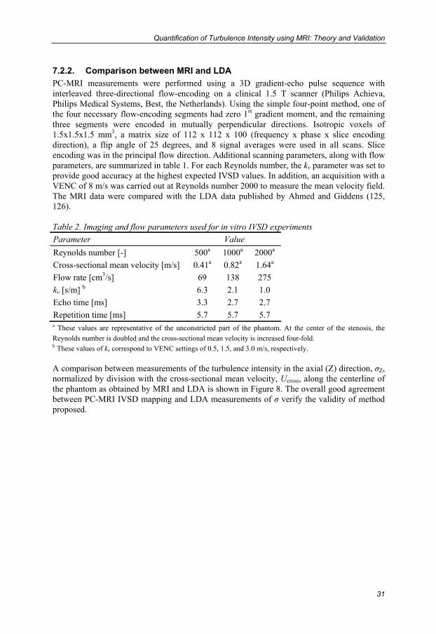
Quantification of Turbulence Intensity using MRI: Theory and Validation
31
7.2.2. Comparison between MRI and LDA PC-MRI measurements were performed using a 3D gradient-echo pulse sequence with interleaved three-directional flow-encoding on a clinical 1.5 T scanner (Philips Achieva, Philips Medical Systems, Best, the Netherlands). Using the simple four-point method, one of the four necessary flow-encoding segments had zero 1st gradient moment, and the remaining three segments were encoded in mutually perpendicular directions. Isotropic voxels of 1.5x1.5x1.5 mm3, a matrix size of 112 x 112 x 100 (frequency x phase x slice encoding direction), a flip angle of 25 degrees, and 8 signal averages were used in all scans. Slice encoding was in the principal flow direction. Additional scanning parameters, along with flow parameters, are summarized in table 1. For each Reynolds number, the kv parameter was set to provide good accuracy at the highest expected IVSD values. In addition, an acquisition with a VENC of 8 m/s was carried out at Reynolds number 2000 to measure the mean velocity field. The MRI data were compared with the LDA data published by Ahmed and Giddens (125, 126). Table 2. Imaging and flow parameters used for in vitro IVSD experiments Parameter Value Reynolds number [-] 500a 1000a 2000a Cross-sectional mean velocity [m/s] 0.41a 0.82a 1.64a Flow rate [cm3/s] 69 138 275 kv [s/m] b 6.3 2.1 1.0 Echo time [ms] 3.3 2.7 2.7 Repetition time [ms] 5.7 5.7 5.7 a These values are representative of the unconstricted part of the phantom. At the center of the stenosis, the Reynolds number is doubled and the cross-sectional mean velocity is increased four-fold. b These values of kv correspond to VENC settings of 0.5, 1.5, and 3.0 m/s, respectively. A comparison between measurements of the turbulence intensity in the axial (Z) direction, σZ, normalized by division with the cross-sectional mean velocity, Ucross, along the centerline of the phantom as obtained by MRI and LDA is shown in Figure 8. The overall good agreement between PC-MRI IVSD mapping and LDA measurements of σ verify the validity of method proposed.

Chapter 7
32
0 1 2 3 4 5 6 7 8 90
0.5
1 Re 500σ
z / U
cros
s [-]
0 1 2 3 4 5 6 7 8 90
0.5
1 Re 1000
σz/U
cros
s [-]
0 1 2 3 4 5 6 7 8 90
0.5
1 Re 2000
σz/U
cros
s [-]
Z [-]
Figure 8. Turbulence intensity along the centerline of the stenosis phantom at Reynolds number 500, 1000, and 2000. MRI measurements (solid lines with markers) are compared with LDA data (circles) published by Ahmed and Giddens (126). Z denotes the distance from the center of the stenosis and has been normalized by the un-occluded pipe diameter. In comparing σ as obtained by MRI and LDA along the centerline of the stenosis phantom, it is apparent that the MRI curve at Reynolds number 2000 is displaced if compared with the LDA curve. The same observation can be made in comparing the mean velocity along the centerline of the phantom, where jet deceleration takes place earlier in the MRI data (Figure 9). This highlights that although great care was taken to mimic the experimental setting used in the LDA measurements, differences are inevitable and therefore the flow fields are different. If compared to the MRI data, the LDA data is sparse and it is difficult to determine the shapes and peak values for σLDA along the centerline at Reynolds number 500 and 1000. LDA measurements of the mean velocity along the centerline were not available for these Reynolds numbers. For Reynolds number 2000, the mean velocity plots indicate that the plateau of constant high-speed flow in the jet that emanates from the stenosis was shorter in the MRI setup if compared to the LDA setup (Figure 9).
0 1 2 3 4 5 6 7 8 90
1
2
3
4
Uz/U
cros
s [-]
Z [-] Figure 9. Mean velocity along the centerline of the stenosis phantom at Reynolds number 2000. MRI measurements (solid lines with markers) are compared with the LDA data (circles) of Ahmed and Giddens (125). Z indicates the distance from the center of the stenosis.

Quantification of Turbulence Intensity using MRI: Theory and Validation
33
7.2.3. Comparison with Computational Fluid Dynamics To permit the assessment of MRI measurements of turbulence intensity on a flow field in which the actual turbulence intensity is known, a PC-MRI simulation method has been developed (128). This simulation method combines time-resolved computational fluid dynamics (CFD) data describing velocity fluctuations with pulse-sequences and RF pulses exported directly from the MRI scanner software. The MRI signal is obtained by solving the Bloch equations using an Eulerian-Lagrangian approach, in which the particle trajectories of virtual spin packets are computed from the time-resolved CFD data. In this way, complete simulations of MRI measurements on fluctuating velocity fields can be made. Figures 10-12 show results of PC-MRI simulations performed on CFD data obtained by large-eddy simulations (7) of the stenosis geometry described above, at Reynolds number 1000. These PC-MRI simulations were carried out using the pulse sequence described in section 7.2.2. The voxel size was 2x2x2 mm3 and kv was set to 2.1. The strong agreement between the turbulence intensity in the CFD data and the full-scale PC-MRI simulations are encouraging and indicate the good accuracy that can be achieved by MRI measurements of turbulence intensity. Included in the plots are also PC-MRI measurements carried out under similar conditions. The shape and peak value of the turbulence intensity along the centerline of the phantom in the measured data agree well with the simulation, apart from an unknown artifact that hampers the PC-MRI measurement data around Z = 3 in Figure 10b. Good agreement is also seen in the images (Figure 11) and plots (Figure 12) of turbulence intensity in a cross section prior to the jet re-attachment zone where fluctuating velocities are present in the jet’s shear layer. All figures show the turbulence intensity in the axial (Z) direction of the phantom. The data in Figure 10 a and b, were obtained with slice- and frequency-encoding in the axial direction, respectively. As described previously, the view-to-view variations that occur in MRI measurements of fluctuating flow cause ghosting artifacts which means that the signal is displaced from its correct position. This artifact occurs primarily in the phase- and slice-encoding directions. As a result, in the geometry used here, σZ as obtained with slice-encoding in the axial direction has higher uncertainty than σZ obtained with frequency-encoding in that direction. In the frequency-encoding direction of the pulse sequence sampling is fast and ghosting artifacts are negligible. On the other hand, the motion encoding and spatial encoding are temporally separated, leading to displacement of the motion-encoded estimates in the resulting image. This effect can be observed in comparing the CFD and simulated PC-MRI data in Figure 10b around Z = 4 where velocity is high. In the phase- and slice-encoding directions, these encodings can be merged or placed closer to each other and displacement is usually negligible. The different effects of artifacts associated with phase-encoding and frequency-encoding are worth taking into account when planning an MRI turbulence intensity measurement.

Chapter 7
34
2 3 4 5 6 7 8 9 100
0.2
0.4
0.6
0.8
1
Z [-]
σz [
m/s
]
CFD
PC-MRI simulationPC-MRI measurement
a
2 3 4 5 6 7 8 9 100
0.2
0.4
0.6
0.8
1
Z [-]
σz [
m/s
]
CFD
PC-MRI simulationPC-MRI measurement
b
Figure 10. Turbulence intensity (σ) along the centerline of a stenotic flow phantom as obtained by PC-MRI simulations (solid lines). The PC-MRI simulations were carried out on CFD data resolving the velocity fluctuations (dotted lines). Shown in the figures are also plots of turbulence intensity as obtained by measurements carried out under similar flow conditions (dashed lines). Subpanels A and B show data obtained with phase- and frequency-encoding in the axial direction (Z), respectively. The horizontal axis show the distance from the center of the stenosis, in the unit of pipe diameters.
Y [
-]
a
-0.5 0 0.5-0.5
0
0.5
X [-]
b
-0.5 0 0.5-0.5
0
0.5c
-0.5 0 0.5-0.5
0
0.5
Figure 11. Turbulence intensity in a cross section of the flow phantom near its re-attachment zone as obtained by CFD (a), PC-MRI simulation (b), and PC-MRI measurement (c). X and Y denote distance from the center of the pipe.

Quantification of Turbulence Intensity using MRI: Theory and Validation
35
-0.5 0 0.50
0.5
1
X [-]
σ z [m/s
]a
-0.5 0 0.50
0.5
1
Y [-]
σ z [m/s
]
b
Figure 12. Turbulence intensity (σ) profiles across the stenotic flow phantom near its re-attachment zone as obtained by PC-MRI simulations (solid lines). The PC-MRI simulations were carried out on CFD data resolving the velocity fluctuations (dotted lines). Shown in the figures are also plots of turbulence intensity as obtained by measurements carried out under similar flow conditions (dashed lines). X and Y denote distance from the center of the pipe.
7.3. Dynamic Range As described in section 7.1, MRI quantification of turbulence intensity using IVSD mapping is based on the signal magnitude ratio between two or more flow-encoding segments acquired with gradient waveforms that differ only in the 1st moment of the bipolar gradients (kv). In this way, factors such as spin density, relaxation effects, and signal void due to magnetic field inhomogeneities caused by the presence of ferromagnetic metal, which are not affected by kv, do not affect the validity of the technique but will affect its dynamic range. Given that one of the two flow-encoding segments needed for IVSD mapping is taken at kv = 0, best sensitivity is obtained if the non-zero measurement is taken where |S(kv)| has its steepest gradient. If σ~ represents a true σ, or a σ-of-interest, this is achieved with kv = 1/σ~ and corresponds to a signal magnitude ratio |S(kv)|/|S(0)| = e-1/2 ≈ 0.6. When σ~ kv << 1, the difference in signal magnitude between S(0) and S(kv) will be poor and estimates of σ will be resolved with lower accuracy. This has previously been pointed out by Kuethe and Gao (58). However, because of the non-zero mean value of MRI magnitude data at low SNR (129, 130), noise may also cause bias.
7.3.1. MRI Magnitude Data at Low SNR When σ~ kv >> 1, the ‘true’ signal magnitude in S(kv) will approach zero. However, as the modulus of S(kv) is used, the effective noise will have a non-zero mean value (129, 130) and the measured signal magnitude will be an overestimation of the ‘true’ magnitude. Consequently, when σ~ kv >> 1, the measured turbulence intensity will be an underestimation of σ~ . Following the approach proposed for diffusion-weighted imaging by Jones and Basser (131), an estimation of the point at which the true signal magnitude equals the mean magnitude of the noise, nm can be obtained simply by replacing |S(kv)| in equation 7.5 by nm. This gives an estimation of σ at which noise on average dominate the measured signal, implying an underestimation of σ:
( )[ ]m/)0(ln2ˆ nSsqrtkσ v = [7.8]
To verify this expression and evaluate its applicability, turbulence intensity measurements with varying kv settings were performed under identical flow settings (Reynolds number 1000) in the stenosis phantom described in section 7.2. For each kv setting, an estimation of

Chapter 7
36
the mean magnitude of the noise was inserted into equation 7.8 to generate estimations of the peak turbulence intensity, σ , that could be measured without on average being underestimated due to noise. As shown in Figure 13, these estimations well represents the peak values of turbulence intensity that could be measured with the different kv settings. Note that for kv = 2.6, the peak values were accurately resolved in the present case.
0 2 4 6 80
0.2
0.4
0.6
0.8
1
]
[m/s
]
Figure 13. The effects of varying the kv parameter in IVSD measurements. The plots show the IVSD, σ, in the axial direction along the centerline of the flow phantom described in section 7.2 with kv set to 5.2 (fat dotted line), 3.5 (dashed) and 2.6 (solid) s/m. The thin horizontal lines show the corresponding peak IVSD value, σ , that could be measured without being underestimated due to noise. The principal flow direction is from left to right. Z denotes the distance from the center of the stenosis and has been normalized by the un-occluded pipe diameter.
7.3.2. Characterization of the Dynamic Range To characterize the impact of noise on the dynamic range of MRI measurements of turbulence intensity, tailor-made simulations were carried out. A theoretically ideal MR signal Stheory(kv·σtrue) was generated by computing equation 7.2 for values of kv·σtrue ranging from 0 to 4.5. Gaussian distributed noise with zero mean and variance 0.0025 was added to the real and the imaginary parts of Stheory(kv·σtrue) to generate a simulated measured signal Smeasured(kv·σtrue) with a maximum SNR of 1/sqrt(0.0025) = 20 for kv·σtrue = 0. In this way, |Smeasured(kv·σtrue)| had a Rician distribution (129) and represented the signal magnitude that for a given combination of kv·σtrue would have been measured at the present SNR. Using equation 7.5, simulated measurements of the turbulence intensity, σmeasured, were obtained for each value of kv·σtrue. This process was repeated 100,000 times to obtain the mean and standard deviation of Smeasured and σmeasured. The dynamic range of MRI measurements of turbulence intensity as characterized using this simulation approach is shown in Figure 14, where the error bars show the uncertainty in the estimates due to noise. If compared to the theoretically ideal MRI signal magnitude |Stheory(kv·σtrue)|, the simulation of the measured signal magnitude |Smeasured(kv·σtrue)| is overestimated at low SNR (upper panel), as predicted. In the lower panel, the turbulence intensity obtained by simulated IVSD mapping, σmeasured, normalized by multiplication with kv, is plotted against kv·σtrue (solid line). When kv·σtrue becomes large, noise dominates the measured signal magnitude and σmeasured approaches σ (dashed line). As predicted by theory, best accuracy is obtained at kv·σ = 1 (circle).

Quantification of Turbulence Intensity using MRI: Theory and Validation
37
0 0.5 1 1.5 2 2.5 3 3.5 40
0.2
0.4
0.6
0.8
1|S
0 0.5 1 1.5 2 2.5 3 3.5 40
1
2
3
4
kv true
k vm
easu
red
Stheory
Smeasured
| |
| |
|
Figure 14. Dynamic range in MRI measurements of turbulence intensity at SNR ≤ 20. The solid lines show the mean of 100,000 estimates and the error bars represent ± one standard deviation. The dotted lines show the theoretical appearance in absence of noise. Upper panel: Compared to the theoretical signal behavior (|Stheory(kvσtrue)|), the measured signal (|Smeasured(kvσtrue)|) is overestimated at low SNR. Lower panel: Measured vs. true turbulence intensity is compared to the theoretical (identity) relation. The dashed line shows the maximum value of kvσmeasured that can be measured without, on average, being underestimated at the present SNR and was computed using equation 7.8. The circle indicates the turbulence intensity measured with lowest uncertainty.
7.3.3. Measurements of Turbulence Intensity using Multiple kv values When more scan time is available, if compared to the case of two kv values for the determination of turbulence intensity in one direction, measurements with multiple kv values or repeated measurements using the same kv values can be applied. If multiple kv values are used, the samples of |S(kv)| may be fitted to the Gaussian curve either in a weighted or non-weighted fashion. To investigate the different strategies for utilizing a given scan time and their effects on the dynamic range, the simulation of two-point turbulence intensity mapping described above was compared with the following approaches that would require a two-fold increase in scan time:
• three averages of S(kv·σtrue = 1), • standard least-squares fit of four measurements of S(kv·σtrue) using four different kv-
values, and • weighted least-squares fit of four measurements of S(kv·σtrue) using four different kv-
values. The weights were empirically set according to a Gaussian filter with standard deviation of 0.2, centered at |S(kv)|/|S(0)| = 0.6.
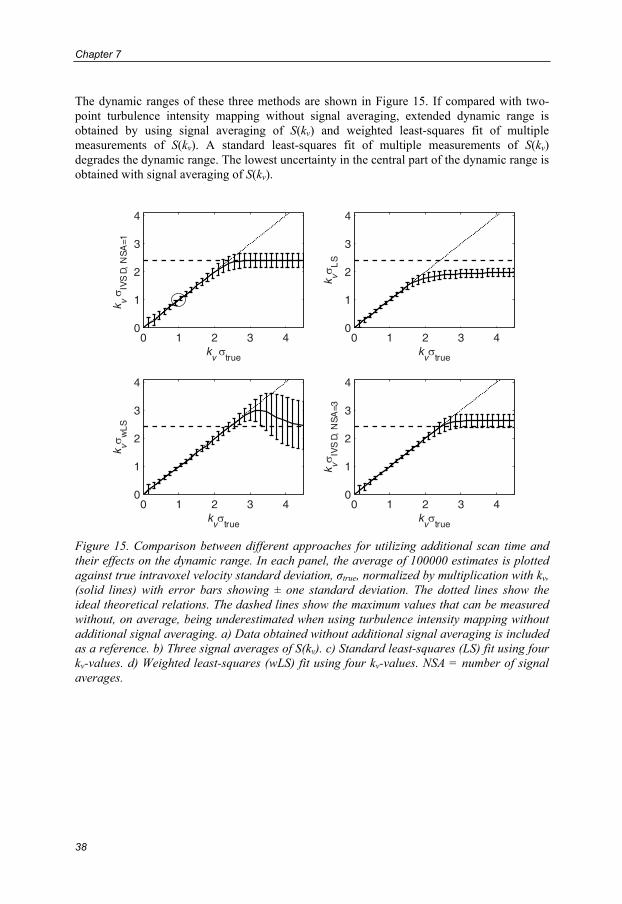
Chapter 7
38
The dynamic ranges of these three methods are shown in Figure 15. If compared with two-point turbulence intensity mapping without signal averaging, extended dynamic range is obtained by using signal averaging of S(kv) and weighted least-squares fit of multiple measurements of S(kv). A standard least-squares fit of multiple measurements of S(kv) degrades the dynamic range. The lowest uncertainty in the central part of the dynamic range is obtained with signal averaging of S(kv).
0 1 2 3 40
1
2
3
4
kv true
k vIV
SD,
NS
A=1
0 1 2 3 40
1
2
3
4
kv true
k vL
S
0 1 2 3 40
1
2
3
4
kv true
k vw
LS
0 1 2 3 40
1
2
3
4
kv true
k vIV
SD,
NS
A=3
Figure 15. Comparison between different approaches for utilizing additional scan time and their effects on the dynamic range. In each panel, the average of 100000 estimates is plotted against true intravoxel velocity standard deviation, σtrue, normalized by multiplication with kv, (solid lines) with error bars showing ± one standard deviation. The dotted lines show the ideal theoretical relations. The dashed lines show the maximum values that can be measured without, on average, being underestimated when using turbulence intensity mapping without additional signal averaging. a) Data obtained without additional signal averaging is included as a reference. b) Three signal averages of S(kv). c) Standard least-squares (LS) fit using four kv-values. d) Weighted least-squares (wLS) fit using four kv-values. NSA = number of signal averages.

Quantification of Turbulence Intensity using MRI: Theory and Validation
39
7.3.4. Guidelines for Setting the kv Parameter With respect to noise, best accuracy in MRI measurements of turbulence intensity is obtained when the product kv·σ equals one, which corresponds to 40% signal loss in S(kv). The kv parameter determines how fast the signal dephases. When σ is low, a strong encoding is necessary to obtain a dephasing that results in a detectable signal loss. If the kv·σ product becomes too small, S(kv) and S(0) will be indistinguishable due to noise. This might not be of great concern to many applications, since uncertainty in low σ values is presumably acceptable when the kv parameter has been set to accurately resolve greater turbulence intensities. In cases where σ is high, kv should be small to prohibit complete signal dephasing. When kv is set too high in relation to the σ values of interest (kv·σ >> 1), S(kv) will loose most of its true signal and will therefore be dominated by noise. Because of the non-zero mean value of low SNR MRI magnitude data this will lead to an overestimation of |S(kv)|, resulting in an underestimation of σ. Using equation 7.8, the influence of noise on the dynamic range can be estimated prior to a measurement to assist in optimizing the parameter settings, as well as retrospectively to assess the dynamic range in an acquired data set. Improved dynamic range assessment may be achieved by reconstructing the data in SNR units (132). The acceptable deviation from kv·σ = 1 depends on the SNR and it is therefore beneficial to maintain a high SNR in the regions of interest. When multiple measurements can be performed, extended dynamic range can be obtained by using signal averaging or by using a weighted fit of multiple measurements of |S(kv)| with different kv settings. When a σ of interest can be approximated, signal averaging may be the best option as it provides the lowest uncertainty in the central parts of the dynamic range. In general, an overall increase in signal magnitude will have beneficial effects on the dynamic range of IVSD mapping and it is therefore important to maintain a high signal-to noise ratio (SNR) in the regions of interest. In order to set the kv parameter so as to obtain good accuracy at the peak σ values in a flow, these values needs to be estimated prior to the measurement. This can be compared to the choice of VENC in PC-MRI velocity mapping, which is commonly made based on prior knowledge of approximate peak velocities in the studied flow condition. Estimation of peak velocities needed to set the VENC in velocity mapping can be obtained from Doppler ultrasound or found in the literature. Corresponding knowledge for values of σ is not yet as widely available; continuing applications of the technique will provide data that ameliorate the choice of kv in future studies.

Chapter 7
40
7.4. On the Assumption of a Specific Intravoxel Velocity Distribution If the intravoxel spin velocity distribution s(u) can be assumed to have a specific distribution, the IVSD can be estimated without directly measuring the second derivative of S(kv) at kv = 0. For the assessment of IVSD in disturbed and turbulent flow, a Gaussian model has been employed. Consequently, errors will occur when s(u) is not Gaussian distributed.
7.4.1. Velocity Distributions in Post-Stenotic Flow To estimate the appearance of s(u) and |S(kv)| in realistic disturbed flow, time-resolved CFD data describing non-pulsatile flow at Reynolds number 2000 in the stenosis geometry (section 7.2) were employed (7). Voxels of 2x2x2 mm3 in the high-resolved CFD flow-field (50 μs temporal resolution, 6 million cells) were considered. To obtain a high spin density, each voxel was sampled at 20 time points which were separated by at least 20 ms. In this way, each voxel comprised about 40000 virtual spins (2000 cells in the CFD mesh x 20 time steps). The intravoxel velocity distribution, s(u), was obtained by computing a probability density estimate of the velocities of the virtual spins within each voxel. From s(u) and the velocities of the virtual spins, S(kv) was computed using equation 4.12. Although based on simulated data of a phantom and computed from a considerably smaller amount of (virtual) spins than what is present in vivo, these distributions may represent reasonable estimates of what can be expected in human cardiovascular blood flow. Representative examples of s(u) and |S(kv)| are shown in Figure 16, and are compared with the Gaussian model. Notably, even though s(u) is not perfectly Gaussian, |S(kv)| is well approximated by the Gaussian model near kv = 0. Deviations from the Gaussian model are most pronounced for large values of kv where the signal amplitude is low. As described in the previous section, this region should be avoided also due to SNR issues. The right column (solid lines) in Figure 16 shows the percentage error in the estimated turbulence intensity resulting from the Gaussian model. The circles indicate the error obtained if the kv parameter is set to match the highest turbulence intensity in the present flow. In the examples shown here this error is less than 4%. The dashed lines in the right column show the percentage error if using the relationship in equation 6.16, which was obtained from a finite difference approximation of the second derivative of S(kv) at kv = 0. These plots reflect that equations 6.16 (valid for only small kv but for arbitrary distributions) and 7.5 (Gaussian model) produce the same result for small kv, as previously shown by Pipe (59).

Quantification of Turbulence Intensity using MRI: Theory and Validation
41
0 1 2
0
50
Rel
. err
or [%
]
kv ˜ [ ]
0 1 2
0
50
Rel
. err
or [%
]
kv ˜ [ ]
0 1 2
0
50
Rel
. err
or [%
]
kv ˜ [ ]
0 1 2
0
50
Rel
. err
or [%
]
kv ˜ [ ]
0 2 4 6 80
0.5
1
u[m/ s]
s(u
)
0 50
0.5
1
kv [m/ s]
|S(k
v)|
0 2 4 6 80
0.5
1
u[m/ s]
s(u
)
0 50
0.5
1
kv [m/ s]
|S(k
v)|
0 2 4 6 80
0.5
1
u[m/ s]
s(u
)
0 50
0.5
1
kv [m/ s]
|S(k
v)|
0 2 4 6 80
0.5
1
u[m/ s]
s(u
)
0 50
0.5
1
kv [m/ s]
|S(k
v)|
Figure 16. s(u) (left column) and |S(kv)| (middle column) in the post-stenotic region of a numerical flow phantom. Solid lines: the actual appearance of s(u) and |S(kv)|. Dotted lines: Gaussian model of s(u) with standard deviation as measured by IVSD mapping and the corresponding |S(kv)|. Right column, solid lines: The percentage error in the IVSD estimation plotted against kv·σ~ , where σ~ is the maximum expected turbulence intensity. The circles indicate the percentage error at the used kv (= 1 / σ~ ). Dashed lines: relative error if using equation 6.16.
7.4.2. Effects of Intravoxel Mean Velocity Variations The presence of intravoxel mean velocity variations, as caused by shear flow or spatial acceleration in a stenosis, will contribute to the intravoxel spin velocity distribution and thereby violate the assumption that s(u) has a Gaussian distribution. Denoting the intravoxel distribution of the mean velocity variations as sMVV(u) and the distribution of the velocity fluctuations as sturb(u), the actual intravoxel spin velocity distribution can be described by the convolution
( ) ( ) ( )ususus turbMVV ∗= [7.9]
which implies that
( ) ( ) ( )vvv kSkSkS turbMVV= [7.10]
where S(kv) is the measured signal.

Chapter 7
42
Rearranging and inserting in equation 7.5 gives
⎥⎥⎦
⎤
⎢⎢⎣
⎡⎟⎟⎠
⎞⎜⎜⎝
⎛−=
)()0(
ln2sqrtMVV
MVV2
2IVSDturb
vv kSS
kσσ [7.11]
where σIVSD is the measured turbulence intensity. This provides a way of estimating, and correcting, for the effects of mean velocity variations on the estimates. The expression predicts that the effects of mean velocity variation decreases with increased turbulence intensity and with increased kv. By approximating the intravoxel mean velocity variations as a linear velocity gradient over a voxel, sMVV(u) can be modeled as a boxcar (uniform) distribution. In this way, the quotient |SMVV(kv)|/|SMVV(0)| becomes |sinc(a kv / 2)|, where a is the velocity difference over the voxel. a can readily be estimated from conventional PC-MRI velocity data. This approach to the estimation of the effects of intravoxel mean velocity variations was applied to the numerical flow phantom described above. Velocity differences of up to 1 m/s over a voxel (2 mm) were present at the site of the stenosis, as shown in Figure 17. Relative to the σ value of interest, defined by σ~ = 1/kv, the maximum contribution from spatial acceleration was less than 3%, in spite of the high acceleration. In the disturbed flow regime around Z = 3, where the elevated values of σIVSD are located, the contribution was less than 1%. Further evaluations of the effects of intravoxel mean velocity variations were made in a range of human cardiovascular disease conditions which will be presented in the next chapter. In disturbed flow regions at sites of aortic coarctation and aortic valve prosthesis, mean velocity variations were estimated to contribute to the measured turbulence intensity by less than 5% in general. Strong vortical flow, giving rise to mean velocity variations within voxels, can be expected to surround the flow jet prior to the reattachment zone in the stenosis phantom. The good accuracy of the turbulence intensity estimates obtained in this regime (Figure 11 and Figure 12) supports the in vivo findings in suggesting that the effect of intravoxel mean velocity variations on MRI measurements of turbulence intensity is negligible. This is also in agreement with previous studies (109).
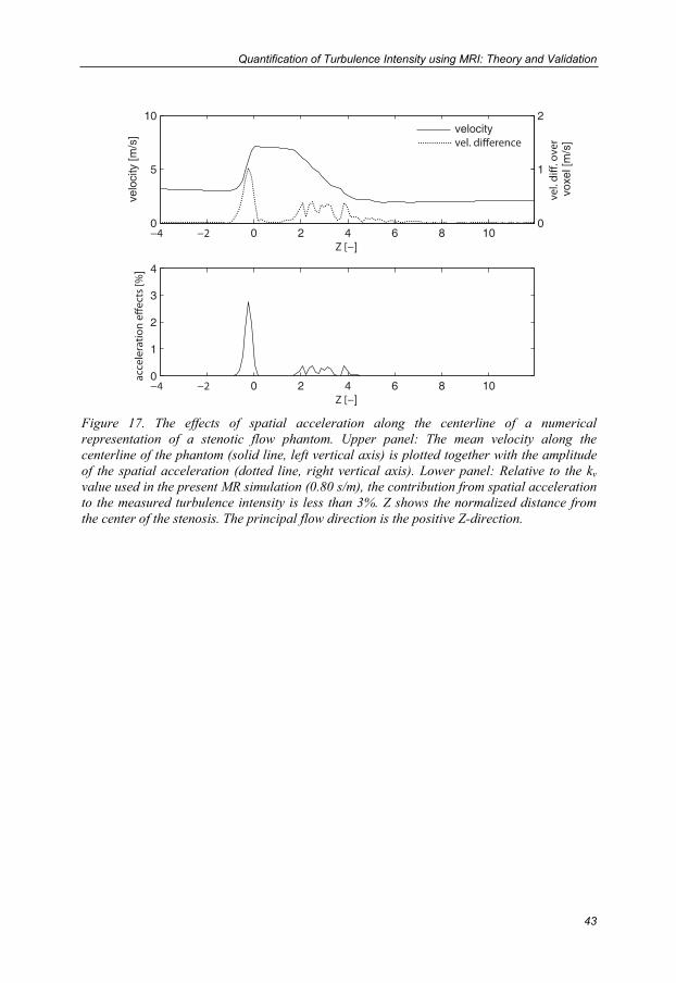
Quantification of Turbulence Intensity using MRI: Theory and Validation
43
0 2 4 6 8 100
5
10
]
velo
city
[m/s
]
0 2 4 6 8 100
1
2
3
4
]
]
0
1
2
voxe
l [m
/s]
velocity
Figure 17. The effects of spatial acceleration along the centerline of a numerical representation of a stenotic flow phantom. Upper panel: The mean velocity along the centerline of the phantom (solid line, left vertical axis) is plotted together with the amplitude of the spatial acceleration (dotted line, right vertical axis). Lower panel: Relative to the kv value used in the present MR simulation (0.80 s/m), the contribution from spatial acceleration to the measured turbulence intensity is less than 3%. Z shows the normalized distance from the center of the stenosis. The principal flow direction is the positive Z-direction.


45
8. Measurements of Turbulence Intensity in
Human Cardiovascular Blood Flow
(Paper III) Extension of IVSD mapping to the quantification of turbulence intensity in the pulsatile blood flow of humans was evaluated by making time-resolved 3D PC-MRI measurements in a range of cardiovascular diseases. Four subjects were included in the study:
• 29-year-old healthy volunteer (male); aortic flow was studied. • 80-year-old male with mild aortic valve regurgitation demonstrated on
echocardiography; left ventricular flow was studied. • 71-year-old male 14 months status post implantation of a stented aortic valve
(Carpentier-Edwards PERIMOUNT, 25 mm diameter). Based on echocardiography, the valve prosthesis had normally opening leaflets and a normal transvalvular pressure gradient. Ascending aortic flow was studied.
• 60-year-old female 46 years status post aortic coarctation repair with an end-to-end anastomosis distal to the left subclavian artery. Signs of restenosis in the anastomosis area were present. In addition, echocardiography also demonstrated the presence of an abnormal minimally obstructive membrane in the left ventricular outflow tract.
8.1. 3D Cine Generalized PC-MRI: Data Acquisition A flow-compensated 3D cine gradient-echo pulse sequence with three-directional flow-encoding was employed. The three-directional flow-encoding scheme consisted of a reference flow-encoding segment, S(0), and a differentially encoded segment, S(kv), in each direction, thus permitting the reconstruction of both the mean velocity and the IVSD in three directions. As in the case of MRI mean velocity mapping, in vivo measurements of turbulence intensity need to be synchronized to the cardiac cycle; this was achieved using vectorcardiogram controlled cardiac gating. Data were acquired during free breathing; to suppress respiratory effects, a navigator gating method was applied. The navigator monitored the position of the diaphragm during the scanning and imaging data were only accepted at end expiration. Without the application of approaches that reduce the scan time, a three-directional 3D cine PC-MRI examination of the human thoracic aorta may take about 40 minutes. To enable a trade-off between the temporal resolution and scan time k-space segmentation was used, implying that multiple k-space lines were acquired per cardiac cycle. With respect to the consideration that maximization of the time between the acquisitions of consecutive k-space lines may be favorable to the sampling of the turbulence scales, the flow-encodes were interleaved to keep the consecutive samples in each flow-encoding segment temporally separated by at least 4 TRs. Further scan time reductions were achieved using parallel imaging by sensitivity encoding (SENSE) (133). All measurements were made on a clinical 1.5 T scanner (Philips Achieva, Philips Medical Systems, Best, the Netherlands).

Chapter 8
46
In all subjects except the coarctation patient, the mean velocity and turbulence intensity of each voxel were reconstructed from the same data set. The kv (VENC) parameter was chosen to provide good accuracy at the highest expected turbulence intensity, which was estimated based on the severity of the disease and velocity estimates available from clinical Doppler ultrasound examinations. In the coarctation patient, an additional scan was made to acquire the mean velocity data. Scanning parameters are summarized in table 2. Table 2. In Vivo Imaging Parameters
Parameter Healthy Volunteer
Aortic Insufficiency
Patient
Valve Prosthesis
Patient
Coarctation Patient, Velocity
Coarctation Patient, IVSD
kv [s/m] 2.24 2.62 1.57 0.90 2.24 Field of View [mm] 278x278x48 300x300x75 300x300x60 272x272x60 288x288x54 Matrix Size 96x 96x16 112x112x24 112x112x20 80x80x20 96x96x18 Echo Time [ms] 3.0 3.0 3.7 3.0 3.0 Repetition Time [ms] 5.2 5.1 6.7 5.4 5.1 SENSE - 2 2 2 - k-space segmentation factor b 3 2 2 3 4
Temporal resolution [ms] 62.4 40.8 53.6 64.8 81.6 Scan Time c 7 min 45 sec 10 min 40 sec 10 min 34 sec 6 min 4 sec 10 min 3 sec a In each of these subjects, both the standard deviation of the intravoxel spin velocity distribution (IVSD) and the velocity were reconstructed from the same data set. b Number of k-space lines (in each of the four flow-encoding segments) acquired per cardiac cycle. c The scan time is exclusive of the navigator gating efficiency.
8.2. Visualization Based on the turbulence intensity in three directions, the direction-independent quantity TKE was computed for each voxel (see section 2.1). The extent and degree of disturbed flow were visualized using surfaces color-coded according to TKE. The surfaces were selected and oriented to encompass the specific regions of interest in each subject. The velocity data were visualized using pathlines and streamlines. Visualizations of streamlines and TKE at the time-point of peak TKE are shown in figures 18-21. These visualizations were made using commercially available software (EnSight, CEI Inc., Apex, NC, United States).
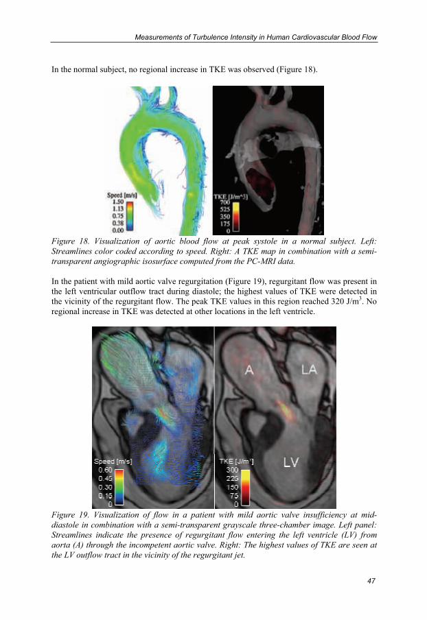
Measurements of Turbulence Intensity in Human Cardiovascular Blood Flow
47
In the normal subject, no regional increase in TKE was observed (Figure 18).
Figure 18. Visualization of aortic blood flow at peak systole in a normal subject. Left: Streamlines color coded according to speed. Right: A TKE map in combination with a semi-transparent angiographic isosurface computed from the PC-MRI data. In the patient with mild aortic valve regurgitation (Figure 19), regurgitant flow was present in the left ventricular outflow tract during diastole; the highest values of TKE were detected in the vicinity of the regurgitant flow. The peak TKE values in this region reached 320 J/m3. No regional increase in TKE was detected at other locations in the left ventricle.
Figure 19. Visualization of flow in a patient with mild aortic valve insufficiency at mid-diastole in combination with a semi-transparent grayscale three-chamber image. Left panel: Streamlines indicate the presence of regurgitant flow entering the left ventricle (LV) from aorta (A) through the incompetent aortic valve. Right: The highest values of TKE are seen at the LV outflow tract in the vicinity of the regurgitant jet.

Chapter 8
48
The systolic flow in the ascending aorta of the patient with aortic valve prosthesis was characterized by high speed flow immediately downstream from the valve and complex flow patterns in the ascending aorta (Figure 20a). Elevated turbulence intensity was detected distal to the prosthesis. The highest values of TKE were present in the central part of the lumen downstream from the valve (Figure 20b). Elevated values of TKE were also observed at the outer wall of the ascending aorta. Peak TKE was about 700 J/m3.
Figure 20. Aortic blood flow at peak systole in a patient with aortic valve prosthesis. Left: Streamlines indicate high-speed flow downstream from the valve and complex flow patterns in the ascending aorta. Right: The highest values of TKE were observed downstream from the valve and at the outer wall of the ascending aorta. In the patient with an aortic coarctation (Figure 21), a distinct flow jet was present distal to the constriction. The highest values of TKE, up to 1000 J/m3, were found downstream from the flow jet; high values were also observed in the jet’s shear-layer. In addition, elevated values of TKE of up to 450 J/m3 were detected in the aortic root downstream from the subvalvular membrane that was present in this patient.
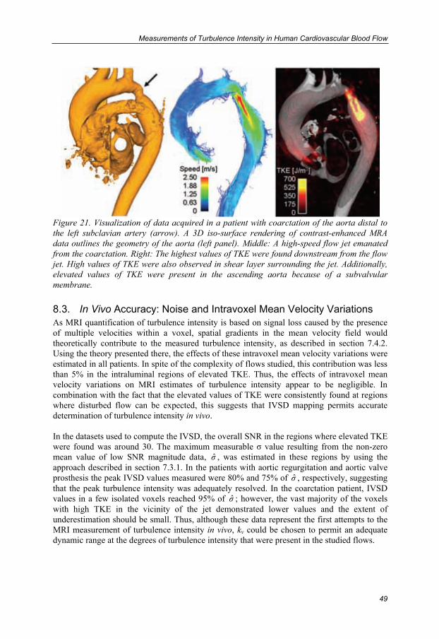
Measurements of Turbulence Intensity in Human Cardiovascular Blood Flow
49
Figure 21. Visualization of data acquired in a patient with coarctation of the aorta distal to the left subclavian artery (arrow). A 3D iso-surface rendering of contrast-enhanced MRA data outlines the geometry of the aorta (left panel). Middle: A high-speed flow jet emanated from the coarctation. Right: The highest values of TKE were found downstream from the flow jet. High values of TKE were also observed in shear layer surrounding the jet. Additionally, elevated values of TKE were present in the ascending aorta because of a subvalvular membrane.
8.3. In Vivo Accuracy: Noise and Intravoxel Mean Velocity Variations As MRI quantification of turbulence intensity is based on signal loss caused by the presence of multiple velocities within a voxel, spatial gradients in the mean velocity field would theoretically contribute to the measured turbulence intensity, as described in section 7.4.2. Using the theory presented there, the effects of these intravoxel mean velocity variations were estimated in all patients. In spite of the complexity of flows studied, this contribution was less than 5% in the intraluminal regions of elevated TKE. Thus, the effects of intravoxel mean velocity variations on MRI estimates of turbulence intensity appear to be negligible. In combination with the fact that the elevated values of TKE were consistently found at regions where disturbed flow can be expected, this suggests that IVSD mapping permits accurate determination of turbulence intensity in vivo. In the datasets used to compute the IVSD, the overall SNR in the regions where elevated TKE were found was around 30. The maximum measurable σ value resulting from the non-zero mean value of low SNR magnitude data, σ , was estimated in these regions by using the approach described in section 7.3.1. In the patients with aortic regurgitation and aortic valve prosthesis the peak IVSD values measured were 80% and 75% of σ , respectively, suggesting that the peak turbulence intensity was adequately resolved. In the coarctation patient, IVSD values in a few isolated voxels reached 95% of σ ; however, the vast majority of the voxels with high TKE in the vicinity of the jet demonstrated lower values and the extent of underestimation should be small. Thus, although these data represent the first attempts to the MRI measurement of turbulence intensity in vivo, kv could be chosen to permit an adequate dynamic range at the degrees of turbulence intensity that were present in the studied flows.


51
9. Investigations of Turbulence Intensity in
Diseased and Prosthetic Heart Valves
Non-invasive time-resolved 3D measurements of turbulence intensity and TKE give access to a class of data that has not previously been accessible in vivo. MRI may also add valuable information to the in vitro assessment of flow, both in medical and engineering applications. While conventional experimental techniques for the in vitro measurement of turbulence intensity are one- or two-dimensional and restricted to specific phantom designs, MRI permit 3D measurements and has few restrictions in terms of phantom design (134).
9.1. Prosthetic Heart Valves (Paper IV) Current prosthetic heart valve designs have proven benefits but continue to fall short of matching the hemodynamics of native heart valves (135). Studies performed both in vitro and in vivo have shown that the flow fields downstream from prosthetic heart valves can be highly disturbed and turbulent (16, 38, 136). To assess the differences in the extent and degree of turbulence intensity in common prosthetic heart valves under similar flow conditions, IVSD mapping was applied in an in vitro setting where stationary flow at 200 cm3/s was flowing through a custom made phantom (Figure 22). Four different aortic valves were studied: Björk-Shiley Monostrut tilting-disc (Shiley Inc, Irvine, CA, United States), St. Jude Medical Standard bileaflet (St. Jude Medical Inc, St Paul, MN, United States), Medtronic Mosaic stented and Medtronic Freestyle stentless porcine (Medtronic Inc, Minneapolis, MN, United States) (Table 3). Separate acquisitions with different kv settings were prescribed to acquire 3D mean velocity (kv = 2.24 s/m ⇔ VENC = 1.40 m/s) and TKE data (kv = 3.49 s/m ⇔ VENC = 0.90 m/s). Isotropic voxels of 2x2x2 mm3 were used in all scans. Distinct differences in the extent and degree of TKE were detected between the four common types of prosthetic valves, as visualized in Figure 22.

Chapter 9
52
Figure 22. Visualizations of the flow fields created by different designs of prosthetic heart valves in a phantom setting. In the background, an isosurface generated from the PC-MRI magnitude data shows the shape of the phantom (dark gray). Sparse streamlines, gray-scale encoded according to speed, outline the mean velocity field. Color-coded isosurfaces generated from the TKE data show the 3D extension of elevated values of TKE (red-yellow-white). The principal flow direction is from left to right in the images. a) Tilting-disc, b) bileaflet, c) stented porcine valve, and d) stentless porcine valve. For each valve, the peak flow speed and the peak TKE were estimated. In addition, a measure of the total flow disorder created by each valve was obtained by integrating the TKE values in the ovoid-shaped chamber downstream from the valve. The integration was done over an equal volume for all valves, starting at the most proximal site where signal void was absent for all four valves, and ending at the site where the oval-shaped outflow chamber ends. These data are presented in table 3. In the present in vitro setting, the peak and total TKE downstream from the valve were not determined by the valves’ effective orifice areas alone. Table 3. Prosthetic heart valves studied and results on velocity and TKE
Björk-Shiley Monostrut®
(Tilting disc)
St. Jude Medical Standard®
(Bileaflet)
Medtronic Mosaic®
(Stented)
Medtronic Freestyle®
(Stentless) Diameter (mm) 27 27 27 27 Effective orifice area (cm2) a 3.34 4.09 2.81 3.75 Maximum flow speed [m/s] 1.0 1.1 1.5 1.1 Peak TKE [J/m3] 100 115 200 145 Total TKE [mJ] 0.9 1.2 2.7 1.4 a In vitro effective orifice area (137).
(a) (b)
(c) (d)
TKE [J/m3] 0 75 150
Speed [m/s] 0.00 0.50 1.00
Investigations of Turbulence Intensity in Diseased and Prosthetic Heart Valves
53
9.2. Mitral Regurgitation (Paper V) The ability of IVSD mapping to enable assessment of the spatiotemporal dynamics of disturbed flow in a specific patient group was investigated in patients with clinically significant mitral valve regurgitation. In mitral regurgitation a high-speed flow jet emanates into the LA at ventricular systole as a result of the incompetent valve. The high-speed jet, contributing both pressure and volume, can cause highly disturbed blood flow in the LA. Seven subjects were included in the study: five patients previously scheduled for mitral valve repair due to prolapse of the middle scallop of the posterior mitral leaflet, and two normal subjects. 3D cine PC-MRI data were acquired using the same basic configuration as described in section 8.1. The kv parameter was set to 2.09 s/m in the patients, which corresponds to a VENC of 1.50 m/s. Rather than attempting to capture the peak velocities in the regurgitant jets, which were estimated to be around 6 m/s by echocardiography, the kv was chosen to provide good accuracy in the turbulence intensity estimates and to permit analysis of flow patterns elsewhere than in the jet. In the normal subjects, a VENC of 1.00 m/s was used. Other scanning parameters included: TR 5.9-6.5 ms, TE 3.4-3.7 ms, flip angle 8°, SENSE reduction factor 2, and voxel size 3x3x3 mm3. Two k-space lines in each flow-encoding segment were acquired per cardiac cycle, resulting in a temporal resolution of about 50 ms. Excluding the navigator gating efficiency, scan time was 10-15 minutes. Both the mean velocity and the turbulence intensity were reconstructed from the single 3D cine PC-MRI dataset acquired in each subject. Based on the turbulence intensity in three directions, the TKE was computed according to equation 2.4. As expected with the VENC set to 1.50 m/s, the velocity data in the high-speed regurgitant jet were aliased, and as a result the jet was not well visualized. Based on previous Doppler ultrasound recordings and the available MRI data, four of the patients had eccentric regurgitant jets directed towards the interatrial septum (Figure 23). One patient had a more central jet. While velocity aliasing occurred in the jet, determination of flow patterns at other intracardiac regions remained feasible (Figure 23).
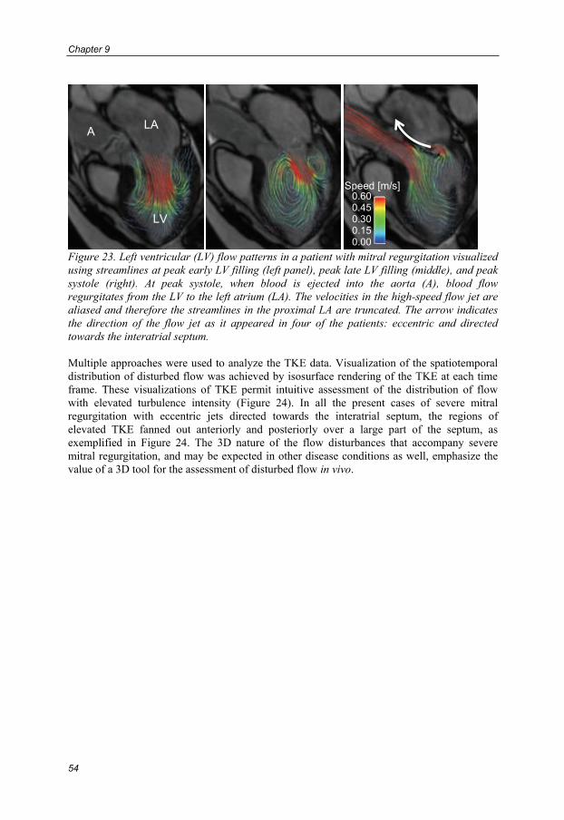
Chapter 9
54
Figure 23. Left ventricular (LV) flow patterns in a patient with mitral regurgitation visualized using streamlines at peak early LV filling (left panel), peak late LV filling (middle), and peak systole (right). At peak systole, when blood is ejected into the aorta (A), blood flow regurgitates from the LV to the left atrium (LA). The velocities in the high-speed flow jet are aliased and therefore the streamlines in the proximal LA are truncated. The arrow indicates the direction of the flow jet as it appeared in four of the patients: eccentric and directed towards the interatrial septum. Multiple approaches were used to analyze the TKE data. Visualization of the spatiotemporal distribution of disturbed flow was achieved by isosurface rendering of the TKE at each time frame. These visualizations of TKE permit intuitive assessment of the distribution of flow with elevated turbulence intensity (Figure 24). In all the present cases of severe mitral regurgitation with eccentric jets directed towards the interatrial septum, the regions of elevated TKE fanned out anteriorly and posteriorly over a large part of the septum, as exemplified in Figure 24. The 3D nature of the flow disturbances that accompany severe mitral regurgitation, and may be expected in other disease conditions as well, emphasize the value of a 3D tool for the assessment of disturbed flow in vivo.
LA A
LV
Speed [m/s] 0.600.450.300.150.00

Investigations of Turbulence Intensity in Diseased and Prosthetic Heart Valves
55
Figure 24. Visualization of the TKE data at late systole in a patient with an eccentric regurgitant jet (upper row) and a patient with a central jet (lower row). Color-coded isosurfaces generated from the TKE data are shown in combination with semi-transparent morphological images in a 3-chamber view (left) and a short-axis view seen from base to apex (right). LV: left ventricle, A: ascending aorta. The data shown in the upper row is typical for all the patients with eccentric jets directed towards the LA septum, where flow with high TKE is distributed over the interatrial septum.
LA
LV
A
600450300150
0
TKE [J/m3]
LA
LV
A
(b) (a)
(d) (c)

Chapter 9
56
A measure of the total extent of LA flow distortion created by the regurgitation was obtained by integrating the TKE over the entire LA volume for all time frames of the cardiac cycle. In terms of the temporal evolution of TKE, the highest values were consistently present at late systole (Figure 25) when the velocities of the mitral regurgitation jet were declining. As expected, TKE was low in the normal subjects (Figure 25). The average LA TKE per cardiac cycle was compared with the regurgitant volume; these quantities appear to relate strongly (Figure 26).
0 20 40 60 80 1000
10
20
30
40
Percentage of RR-interval [%]
Tot
al T
KE
[m
J]
normals
patients
Figure 25. Temporal evolution of the total TKE in the left atrium. In the normal subjects (dashed lines), the TKE is low throughout the cardiac cycle. The mitral regurgitant patients (solid lines) demonstrate marked increases in TKE over a large part of the cardiac cycle, with peak values occurring in late systole. The horizontal axis indicates the time in the cardiac cycle, expressed as the percentage of the RR-interval. Ventricular systole comprises the initial 35-40% of the cardiac cycle.
0 20 40 60 800
2
4
6
8
10
12
14
16
18
Regurgitant volume [ml]
Ave
rage
TK
E f
or o
ne h
eart
beat
[m
J]
normals
patients
Figure 26. The average TKE in the left atrium over one cardiac cycle plotted against the regurgitant volume for each subject. The average TKE was obtained by taking the sum of the total TKE for all time frames in one cardiac cycle and dividing by the number of time frames.
57
10. Discussion
In this thesis, a method for the non-invasive quantification of turbulence intensity has been presented. This method addresses a long-standing gap in the scientific and clinical armamentarium for assessing and understanding cardiovascular diseases, which are often accompanied by disturbed and turbulent flow. The turbulence intensity corresponds to the standard deviation of the flow velocity fluctuations that are present in such flows. As described in paper I, the proposed method quantifies turbulence intensity via a measurement of the IVSD by exploiting the effects of velocity fluctuations on the MRI signal. Conventionally, fluid mechanics experiments based on optical and thermal anemometry measure turbulence intensity by sampling the velocity in the temporal domain. In MRI, spatiotemporal sampling is performed. When the flow is ergodic and the turbulence scales are adequately sampled, turbulence intensity as obtained by IVSD mapping is equivalent to optical and thermal anemometry, assuming that those methods are adequately applied. In this thesis, the proposed MRI method for quantification of turbulence intensity is validated using theoretical, numerical, and experimental approaches. In addition, findings that support the potential of MRI quantification of turbulence intensity have recently been reported by Elkins et al. (118). Several potential sources of error in MRI quantification of turbulence intensity were investigated in paper II. The approach for the assessment of the dynamic range of IVSD mapping presented there provides a means to assess the uncertainty in measured turbulence intensity estimates. Further, an approach to estimate, and correct for, the effects of signal loss caused by intravoxel mean velocity variations was presented and applied to data obtained by MRI simulations as well as in vivo measurements. The findings demonstrated that the contribution of intravoxel mean velocity variations to the measured turbulence intensity value is negligible compared to the effects of velocity fluctuations. In paper III, turbulence intensity data were acquired across a spectrum of cardiovascular diseases; these data represent the first ever time-resolved 3D turbulence intensity measurements in humans and demonstrate the in vivo feasibility of the technique. Application studies performed in vitro (paper IV) and in vivo (paper V) demonstrate the technique’s potential for assessment of disturbed and turbulent flow in prosthetic devices and advanced cardiovascular disease.

Chapter 10
58
10.1. Moment Framework MRI has several important applications in the assessment of cardiovascular blood flow but might not yet have reached its full potential. The most common MRI method for the assessment of flow measures the mean velocity of a voxel under the assumption that the velocity distribution within the voxel is symmetric about its mean. The mean velocity corresponds to the first raw moment of the intravoxel spin velocity distribution. As described in this thesis, MRI has the potential to quantify any moment (mean, standard deviation, skew, etc.) of arbitrary intravoxel spin velocity distributions. As a first application of this framework, a method for the quantification of turbulence intensity has been developed. By permitting interpretations of different operations and quantification problems in both the velocity domain and the transform domain, the moment framework may prove to be fertile ground for the development of new MRI methods for the quantification of hemodynamic parameters. The framework may also be of help in the refinement of existing methods. The method for quantification of turbulence intensity presented in this thesis employs a Gaussian model of s(u) to determine the IVSD in disturbed and turbulent flows. As described in paper I, several other distributions may be used as well. In laminar flow regions, where velocity fluctuations are absent, the effects of spatial acceleration may be exploited to study fluid mechanical parameters other than turbulence intensity. High spatial acceleration is typical for flow near the vessel wall and it has previously been suggested that the concomitant signal loss could be used to estimate the wall shear stress (59), which is one of the fluid mechanical stresses that acts on the vessel wall. The wall shear stress is given by the wall shear rate multiplied by the dynamic viscosity of the fluid. Acting directly on the vessel wall, the wall shear stress has been implicated in the pathogenesis of atherosclerosis (138, 139). Several methods for the assessment of wall shear stress based on extrapolation of MRI velocity data have been proposed but are highly sensitive to spatial resolution and partial volume artifacts (140-142). Additionally, the estimates of wall shear rate derived from MRI velocity data might not always be related to the actual wall shear rate (143). By resolving velocities on a subvoxel level, the FVE-MRI approach (105, 106) mentioned in section 4.4.2 addresses many of the limitations associated with WSS assessment based on mean velocity data. Using the moment framework, estimations of the statistical dispersion of the intravoxel velocity distribution near the vessel wall, rather than in fluctuating intraluminal flow, may be achieved by applying a model that is tailored to the expected flow field; this approach is currently under investigation. In addition, partial volume effects may potentially be accounted for by extending the model and utilize multiple measurements of S(kv). This would permit wall shear rate estimations in voxels that contain both flowing blood and vessel wall.
10.2. Future Work As the technique has not yet been widely applied, there are most likely several opportunities for improving the MRI quantification of turbulence intensity and tailoring the data acquisition to the specific question.
10.2.1. Scan Time The relatively long scan time of 3D cine PC-MRI may hamper its utility in large scale studies and clinical applications. 2D measurements of turbulence intensity may be an option when a full 3D coverage of the flow of interest is not necessary. However, in 2D MRI, spins with different velocities and different motion trajectories may experience a different number of RF
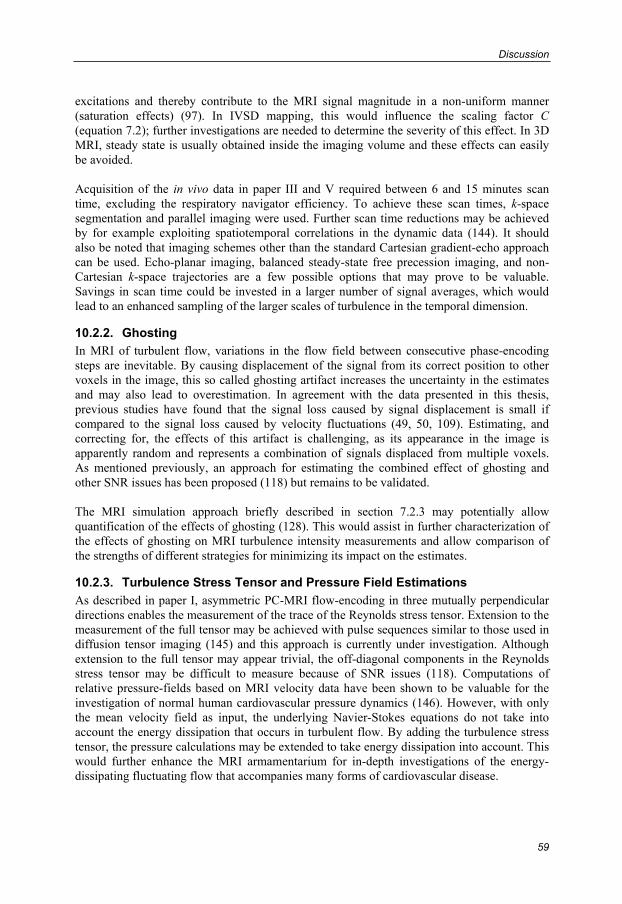
Discussion
59
excitations and thereby contribute to the MRI signal magnitude in a non-uniform manner (saturation effects) (97). In IVSD mapping, this would influence the scaling factor C (equation 7.2); further investigations are needed to determine the severity of this effect. In 3D MRI, steady state is usually obtained inside the imaging volume and these effects can easily be avoided. Acquisition of the in vivo data in paper III and V required between 6 and 15 minutes scan time, excluding the respiratory navigator efficiency. To achieve these scan times, k-space segmentation and parallel imaging were used. Further scan time reductions may be achieved by for example exploiting spatiotemporal correlations in the dynamic data (144). It should also be noted that imaging schemes other than the standard Cartesian gradient-echo approach can be used. Echo-planar imaging, balanced steady-state free precession imaging, and non-Cartesian k-space trajectories are a few possible options that may prove to be valuable. Savings in scan time could be invested in a larger number of signal averages, which would lead to an enhanced sampling of the larger scales of turbulence in the temporal dimension.
10.2.2. Ghosting In MRI of turbulent flow, variations in the flow field between consecutive phase-encoding steps are inevitable. By causing displacement of the signal from its correct position to other voxels in the image, this so called ghosting artifact increases the uncertainty in the estimates and may also lead to overestimation. In agreement with the data presented in this thesis, previous studies have found that the signal loss caused by signal displacement is small if compared to the signal loss caused by velocity fluctuations (49, 50, 109). Estimating, and correcting for, the effects of this artifact is challenging, as its appearance in the image is apparently random and represents a combination of signals displaced from multiple voxels. As mentioned previously, an approach for estimating the combined effect of ghosting and other SNR issues has been proposed (118) but remains to be validated. The MRI simulation approach briefly described in section 7.2.3 may potentially allow quantification of the effects of ghosting (128). This would assist in further characterization of the effects of ghosting on MRI turbulence intensity measurements and allow comparison of the strengths of different strategies for minimizing its impact on the estimates.
10.2.3. Turbulence Stress Tensor and Pressure Field Estimations As described in paper I, asymmetric PC-MRI flow-encoding in three mutually perpendicular directions enables the measurement of the trace of the Reynolds stress tensor. Extension to the measurement of the full tensor may be achieved with pulse sequences similar to those used in diffusion tensor imaging (145) and this approach is currently under investigation. Although extension to the full tensor may appear trivial, the off-diagonal components in the Reynolds stress tensor may be difficult to measure because of SNR issues (118). Computations of relative pressure-fields based on MRI velocity data have been shown to be valuable for the investigation of normal human cardiovascular pressure dynamics (146). However, with only the mean velocity field as input, the underlying Navier-Stokes equations do not take into account the energy dissipation that occurs in turbulent flow. By adding the turbulence stress tensor, the pressure calculations may be extended to take energy dissipation into account. This would further enhance the MRI armamentarium for in-depth investigations of the energy-dissipating fluctuating flow that accompanies many forms of cardiovascular disease.

Chapter 10
60
10.3. Potential Impact
10.3.1. Engineering Flows Non-invasive measurements of turbulence intensity in 3D may prove to be a valuable resource also beyond the field of cardiovascular medicine. In many engineering flow applications, the multidimensional and multidirectional turbulence intensity data obtainable with MRI, in combination with its minimal restrictions in terms of phantom design, can add to the data currently obtained by LDA and PIV (116).
10.3.2. Valvular Disease In paper IV, IVSD mapping was applied to measure turbulence intensity in the flow fields created by common designs of prosthetic heart valves. Distinct differences in the extent, location, and degree of turbulence intensity were detected. Paper III included data on TKE in a patient with a stented aortic valve prosthesis. Further investigation of prosthetic valve-associated TKE in vivo may allow the in vitro findings to be extended to representative conditions of pulsatile flow and anatomic surroundings. This may provide novel information regarding how to optimize prosthetic valve performance with best approaches to surgical implantation and anatomic orientation (147, 148). In paper V, time-resolved 3D measurements of turbulence intensity were made in the left heart of patients with clinically significant mitral regurgitation. The results of that study, which represents the first application of MRI turbulence intensity measurements to a specific patient group, suggest that the total TKE in the left atrium is closely related to the regurgitation volume.
10.3.3. Blood Trauma The fluid mechanical forces in turbulent flows may have important effects on blood constituents (149). In vitro experiments and studies performed in animal models have provided data that support that turbulent flow can cause hemolysis (20, 21) and platelet activation (22) and that there might exist thresholds for when this occurs. Thresholds based on measurements of the TKE or the complete Reynolds stress tensor would permit in vivo risk stratification of hemolysis and platelet activation.
10.3.4. Atherosclerosis Hemodynamic forces regulate endothelial cell function, and turbulent flow has been correlated with endothelial processes leading to atherosclerosis (28, 150). Non-invasive correlation of turbulence intensity with endothelial responses such as surface receptor and gene alterations would open new avenues for disease recognition and management of patients at risk for the development and progression of atherosclerosis. In the advanced stages of atherosclerosis, vulnerable stenotic plaques are at risk for rupture. Stenotic plaques which create similar degrees of constriction but which have different shapes will cause different stresses on the vessel wall (151). This suggests that the risk of plaque progression and rupture might also differ with the specific plaque geometry. The decision to operate on asymptomatic stenotic plaques is currently based on the degree of stenosis rather than any other morphologic characteristic of the plaque. This incongruity may largely be attributed to the lack of clinical tools for studying the hemodynamic impact of specific stenoses. Measurements of turbulence intensity may help in characterizing the specific distortions created by a stenosis in vivo (Figure 27) (152), and lead to a more reliable approach to selecting patients with the most to gain from surgical endarterectomy.
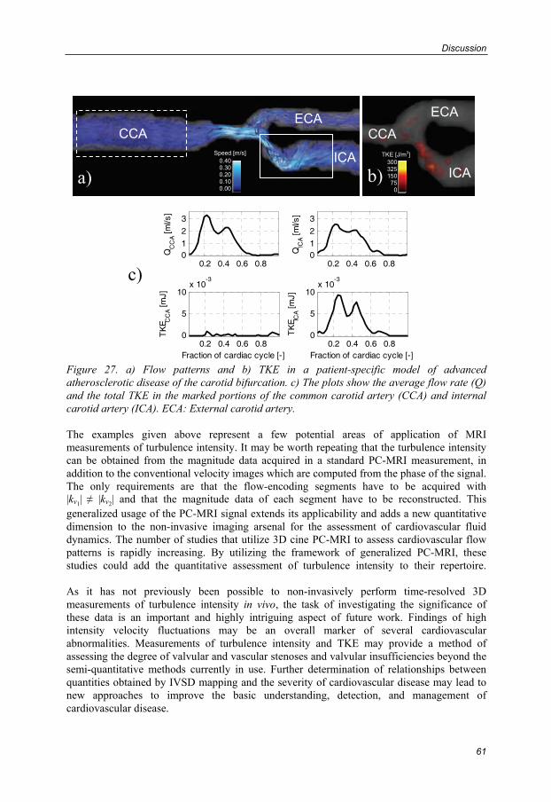
Discussion
61
Figure 27. a) Flow patterns and b) TKE in a patient-specific model of advanced atherosclerotic disease of the carotid bifurcation. c) The plots show the average flow rate (Q) and the total TKE in the marked portions of the common carotid artery (CCA) and internal carotid artery (ICA). ECA: External carotid artery. The examples given above represent a few potential areas of application of MRI measurements of turbulence intensity. It may be worth repeating that the turbulence intensity can be obtained from the magnitude data acquired in a standard PC-MRI measurement, in addition to the conventional velocity images which are computed from the phase of the signal. The only requirements are that the flow-encoding segments have to be acquired with |kv1| ≠ |kv2| and that the magnitude data of each segment have to be reconstructed. This generalized usage of the PC-MRI signal extends its applicability and adds a new quantitative dimension to the non-invasive imaging arsenal for the assessment of cardiovascular fluid dynamics. The number of studies that utilize 3D cine PC-MRI to assess cardiovascular flow patterns is rapidly increasing. By utilizing the framework of generalized PC-MRI, these studies could add the quantitative assessment of turbulence intensity to their repertoire. As it has not previously been possible to non-invasively perform time-resolved 3D measurements of turbulence intensity in vivo, the task of investigating the significance of these data is an important and highly intriguing aspect of future work. Findings of high intensity velocity fluctuations may be an overall marker of several cardiovascular abnormalities. Measurements of turbulence intensity and TKE may provide a method of assessing the degree of valvular and vascular stenoses and valvular insufficiencies beyond the semi-quantitative methods currently in use. Further determination of relationships between quantities obtained by IVSD mapping and the severity of cardiovascular disease may lead to new approaches to improve the basic understanding, detection, and management of cardiovascular disease.
a)
CCA
ICA
ECA
b)
CCA
ICA
ECA
0.2 0.4 0.6 0.801
2
3
QC
CA [m
l/s]
0.2 0.4 0.6 0.801
2
3
QIC
A [m
l/s]
0.2 0.4 0.6 0.80
5
10x 10
-3
TK
E CC
A [m
J]
Fraction of cardiac cycle [-]0.2 0.4 0.6 0.8
0
5
10x 10
-3
TK
E ICA [m
J]
Fraction of cardiac cycle [-]
c)
30032515075
0
TKE [J/m3] 0.400.300.200.100.00
Speed [m/s]

63
Bibliography
1. Causes of Death 2007. The National Board of Health and Welfare (Socialstyrelsen), Centre for Epidemiology; 2009 [cited 2009 Oct 27]. Available from: http://www.socialstyrelsen.se.
2. Lopez AD, Mathers CD, Ezzati M, Jamison DT, Murray CJL. Global and regional burden of disease and risk factors, 2001: systematic analysis of population health data. The Lancet 2006;367(9524):1747-1757.
3. Yoganathan AP, Chandran KB, Sotiropoulos F. Flow in prosthetic heart valves: state-of-the-art and future directions. Annals of Biomedical Engineering 2005;33(12):1689-94.
4. Richter Y, Edelman ER. Cardiology Is Flow. Circulation 2006;113:2679-2682.
5. Hinze JO. Turbulence. New York: McGraw-Hill; 1975.
6. Mathieu J, Scott J. An Introduction to Turbulent Flow. Cambridge: Cambridge University Press; 2000.
7. Gårdhagen R, Lantz J, Carlsson F, Karlsson M. Large eddy simulation of flow through a stenosed pipe. In: American Society of Mechanical Engineers Summer Bioengineering Conference; 2008; Marco Island, Florida, United States.
8. Reynolds O. An experimental investigation of the circumstances which determine whether the motion of water shall be direct or sinuous, and of the law of resistance in parallel channels. Philosophical Transactions of the Royal Society of London 1883;174:935-982.
9. Yellin EL. Laminar-turbulent transition process in pulsatile flow. Circulation Research 1966;19(4):791-804.
10. Romane GP, Ouellette NT, Xu H, Bodenschatz E, Steinberg V, Meneveau C, Katz J. Measurements of Turbulent Flow. In: Tropea C, Yarin AL, Foss JF, editors. Handbook of Experimental Fluid Mechanics. Berlin: Springer-Verlag; 2007.
11. Deissler RG. Turbulent fluid motion. Philadelphia: Taylor and Francis; 1998.
12. Comte-Bellot G. Hot-wire anemometry. Annual Review of Fluid Mechanics 1976;8(1):209-231.
13. Buchhave P, George Jr WK, Lumley JL. The measurement of turbulence with the laser-Doppler anemometer. Annual Review of Fluid Mechanics 1979;11(1):443-503.
14. Westerweel J. Fundamentals of digital particle image velocimetry. Measurement Science and Technology 1997;8:1379-1392.

Bibliography
64
15. Tavoularis S. Measurement in fluid mechanics. New York: Cambridge University Press; 2005.
16. Stein PD, Sabbah HN. Turbulent blood flow in the ascending aorta of humans with normal and diseased aortic valves. Circulation Research 1976;39(1):58-65.
17. Ku DN. Blood flow in arteries. Annual Review of Fluid Mechanics 1997;29(1):399-434.
18. Nichols W, O'Rourke M. McDonald's Blood Flow in Arteries. 5th ed. London: Hodder Arnold; 2005.
19. Sutera SP, Mehrjardi MH. Deformation and fragmentation of human red blood cells in turbulent shear flow. Biophysical Journal 1975;15(1):1-10.
20. Sallam AM, Hwang NH. Human red blood cell hemolysis in a turbulent shear flow: contribution of Reynolds shear stresses. Biorheology 1984;21(6):783-97.
21. Kameneva MV, Burgreen GW, Kono K, Repko B, Antaki JF, Umezu M. Effects of turbulent stresses upon mechanical hemolysis: experimental and computational analysis. American Society for Artificial Organs (ASAIO) Journal 2004;50(5):418-423.
22. Stein PD, Sabbah HN. Measured turbulence and its effect on thrombus formation. Circulation Research 1974;35(4):608-614.
23. Becker RC, Eisenberg P, Turpie AG. Pathobiologic features and prevention of thrombotic complications associated with prosthetic heart valves: fundamental principles and the contribution of platelets and thrombin. American Heart Journal 2001;141(6):1025-1037.
24. Davies PF, Remuzzi A, Gordon EJ, Dewey CF, Gimbrone Jr MA. Turbulent fluid shear stress induces vascular endothelial cell turnover in vitro. Proceedings of the National Academy of Sciences 1986;83(7):2114-2117.
25. Malek AM, Alper SL, Izumo S. Hemodynamic shear stress and its role in atherosclerosis. Journal of the American Medical Association 1999;282(21):2035-2042.
26. Gimbrone Jr MA, Topper JN, Nagel T, Anderson K, Garcia-Cardena G. Endothelial dysfunction, hemodynamic forces, and atherogenesis. Annals of the New York Academy of Sciences 2000;902:230-240.
27. VanderLaan PA, Reardon CA, Getz GS. Site specificity of atherosclerosis: site-selective responses to atherosclerotic modulators. Arteriosclerosis Thrombosis and Vascular Biology 2004;24(1):12-22.
28. Brooks AR, Lelkes PI, Rubanyi GM. Gene expression profiling of vascular endothelial cells exposed to fluid mechanical forces: relevance for focal susceptibility to atherosclerosis. Endothelium 2004;11(1):45-57.
Bibliography
65
29. Cheng C, Tempel D, van Haperen R, van der Baan A, Groseveld F, Daemen MJAP, Kramp R, de Crom R. Atherosclerotic lesion size and vulnerability are determined by patterns of fluid shear stress. Circulation 2006;113:2744-2753.
30. Wakhloo AK, Lieber BB, Seong J, Sadasivan C, Gounis MJ, Miskolczi L, Sandhu JS. Hemodynamics of carotid artery atherosclerotic occlusive disease. Journal of Vascular and Interventional Radiology 2004;15(1 Pt 2):S111-121.
31. Falk E, Shah PK, Fuster V. Coronary plaque disruption. Circulation 1995;92(3):657-671.
32. Sabbah H, Stein P. Turbulent blood flow in humans: its primary role in the production of ejection murmurs. Circulation Research 1976;38(6):513-525.
33. Fung YC. Biodynamics: Circulation. New York: Springer-Verlag; 1984.
34. Nerem RM, Seed WA. An in vivo study of aortic flow disturbances. Cardiovascular Research 1972;6(1):1-14.
35. Peacock J, Jones T, Tock C, Lutz R. The onset of turbulence in physiological pulsatile flow in a straight tube. Experiments in Fluids 1998;24(1):1-9.
36. Seed W, Wood N. Velocity patterns in the aorta. Cardiovascular Research 1971;5(3):319-330.
37. Nygaard H, Hasenkam JM, Pedersen EM, Kim WY, Paulsen PK. A new perivascular multi-element pulsed Doppler ultrasound system forin vivo studies of velocity fields and turbulent stresses in large vessels. Medical and Biological Engineering and Computing 1994;32(1):55-62.
38. Nygaard H, Paulsen PK, Hasenkam JM, Pedersen EM, Rovsing PE. Turbulent stresses downstream of three mechanical aortic valve prostheses in human beings. Journal of Thoracic and Cardiovascular Surgery 1994;107:438-446.
39. Cloutier G, Allard L, Durand LG. Characterization of blood flow turbulence with pulsed-wave and power Doppler ultrasound imaging. Journal of Biomechanical Engineering 1996;118(3):318-325.
40. Cloutier G, Chen D, Durand LG. Performance of time-frequency representation techniques to measure blood flow turbulence with pulsed-wave Doppler ultrasound. Ultrasound in Medicine and Biology 2001;27(4):535-550.
41. Poepping TL, Nikolov HN, Rankin RN, Lee M, Holdsworth DW. An in vitro system for Doppler ultrasound flow studies in the stenosed carotid artery bifurcation. Ultrasound in Medicine and Biology 2002;28(4):495-506.
42. Isaaz K, Bruntz JF, Da Costa A, Winninger D, Cerisier A, de Chillou C, Sadoul N, Lamaud M, Ethevenot G, Aliot E. Noninvasive quantitation of blood flow turbulence in patients with aortic valve disease using online digital computer analysis of Doppler velocity data. Journal of the American Society of Echocardiography 2003;16(9):965-974.

Bibliography
66
43. Wong EY, Nikolov HN, Thorne ML, Poepping TL, Rankin RN, Holdsworth DW. Clinical Doppler ultrasound for the assessment of plaque ulceration in the stenosed carotid bifurcation by detection of distal turbulence intensity: a matched model study. European Radiology 2009;19(11):2739-2749.
44. Grigioni M, Daniele C, D'Avenio G, Barbaro V. On the monodimensional approach to the estimation of the highest reynolds shear stress in a turbulent flow. Journal of Biomechanics 2000;33(6):701-708.
45. Ståhlberg F, Ericsson A, Nordell B, Thomsen C, Henriksen O, Persson BR. MR imaging, flow and motion. Acta Radiologica 1992;33(3):179-200.
46. Gatehouse PD, Keegan J, Crowe LA, Masood S, Mohiaddin RH, Kreitner KF, Firmin DN. Applications of phase-contrast flow and velocity imaging in cardiovascular MRI. Eur Radiol 2005;15(10):2172-2184.
47. Hope TA, Herfkens RJ. Imaging of the Thoracic Aorta with Time-Resolved Three-Dimensional Phase-Contrast MRI: A Review. Seminars in thoracic and cardiovascular surgery 2008;20(4):358-364.
48. Evans AJ, Blinder RA, Herfkens RJ, Spritzer CE, Kuethe DO, Fram EK, Hedlund LW. Effects of turbulence on signal intensity in gradient echo images. Investigative Radiology 1988;23(7):512-518.
49. Gatenby JC, McCauley TR, Gore JC. Mechanisms of signal loss in magnetic resonance imaging of stenoses. Medical Physics 1993;20(4):1049-1057.
50. Oshinski JN, Ku DN, Pettigrew RI. Turbulent fluctuation velocity: the most significant determinant of signal loss in stenotic vessels. Magnetic Resonance in Medicine 1995;33(2):193-199.
51. de Gennes PG. Theory of Spin Echoes in a Turbulent Fluid. Physics Letters 1969;29A(1):20-21.
52. Fukuda K, Hirai A. A pulsed NMR study on the flow of fluid. Journal of the Physical Society of Japan 1979;47:1999-2006.
53. Nalcioglu O, Cho Z, Xiang Q, Ahn C. Incoherent flow imaging. In: International Workshop on Physics and Engineering of Computerized Multidimensional Imaging and Processing; 1986; Newport Beach, California, United States. p. 285-289.
54. Xiang QS, Nalcioglu O. Measurement of mean and variance of velocity fields within each voxel by NMR imaging. IEEE transactions on medical imaging 1988;7(4):364-367.
55. Kuethe DO. Measuring distributions of diffusivity in turbulent fluids with magnetic-resonance imaging. Physical Review A 1989;40(8):4542-4551.
56. Gao JH, Gore JC. Turbulent flow effects on NMR imaging: measurement of turbulent intensity. Medical Physics 1991;18(5):1045-1051.
57. Gatenby JC, Gore JC. Mapping of turbulent intensity by magnetic resonance imaging. Journal of Magnetic Resonance B 1994;104(2):119-126.
Bibliography
67
58. Kuethe DO, Gao JH. NMR signal loss from turbulence: Models of time dependence compared with data. Physical Review E 1995;51(4):3252-3262.
59. Pipe JG. A simple measure of flow disorder and wall shear stress in phase contrast MRI. Magnetic Resonance in Medicine 2003;49(3):543-550.
60. Rabi II, Zacharias JR, Millman S, Kusch P. A new method of measuring nuclear magnetic moment. Physical Review 1938;53(4):318-318.
61. Bloch F. Nuclear induction. Physical Review 1946;70(7-8):460-474.
62. Purcell EM, Torrey HC, Pound RV. Resonance absorption by nuclear magnetic moments in a solid. Physical Review 1946;69(1-2):37-38.
63. Lauterbur PC. Image Formation by Induced Local Interactions: Examples Emloying Nuclear Magnetic Resonance. Nature 1973;242:190-191.
64. Lauterbur PC. Magnetic Resonance Zeugmatography. Pure and Applied Chemistry 1974:149-157.
65. Mansfield P. Multi-planar image formation using NMR spin echoes. Journal of Physics C 1977;10(L55):349-352.
66. Twieg D. The k-trajectory formulation of the NMR imaging process with applications in analysis and synthesis of imaging methods. Medical Physics 1983;10(5):610-621.
67. Ljunggren S. A simple graphical representation of Fourier-based imaging methods. Journal of Magnetic Resonance 1983;54(2):338-343.
68. Lanzer P, Barta C, Botvinick EH, Wiesendanger HU, Modin G, Higgins CB. ECG-synchronized cardiac MR imaging: method and evaluation. Radiology 1985;155(3):681-686.
69. Glover GH, Pelc NJ. A rapid-gated cine MRI technique. Magnetic Resonance Annual 1988:299-333.
70. Bryant DJ, Payne JA, Firmin DN, Longmore DB. Measurement of flow with NMR imaging using a gradient pulse and phase difference technique. Journal of Computer Assisted Tomography 1984;8(4):588-593.
71. van Dijk P. Direct cardiac NMR imaging of heart wall and blood flow velocity. Journal of Computer Assisted Tomography 1984;8(3):429-436.
72. Moran PR. A flow velocity zeugmatographic interlace for NMR imaging in humans. Magnetic Resonance Imaging 1982;1(4):197-203.
73. Redpath TW, Norris DG, Jones RA, Hutchison JM. A new method of NMR flow imaging. Physics in Medicine and Biology 1984;29(7):891-895.
74. Hamilton CA, Moran PR, Santago P, 2nd, Rajala SA. Effects of intravoxel velocity distributions on the accuracy of the phase-mapping method in phase-contrast MR angiography. Journal of Magnetic Resonance Imaging 1994;4(5):752-755.
Bibliography
68
75. Xiang QS. Temporal phase unwrapping for CINE velocity imaging. Journal of Magnetic Resonance Imaging 1995;5(5):529-534.
76. Pelc NJ, Herfkens RJ, Shimakawa A, Enzmann DR. Phase contrast cine magnetic resonance imaging. Magnetic Resonance Quarterly 1991;7(4):229-254.
77. Nayler GL, Firmin DN, Longmore DB. Blood flow imaging by cine magnetic resonance. Journal of Computer Assisted Tomography 1986;10(5):715-722.
78. Pennell DJ, Sechtem UP, Higgins CB, Manning WJ, Pohost GM, Rademakers FE, van Rossum AC, Shaw LJ, Kent Yucel E. Clinical Indications for Cardiovascular Magnetic Resonance (CMR): Consensus Panel Report. Journal of Cardiovascular Magnetic Resonance 2004;6(4):727-765.
79. Hendel RC, Patel MR, Kramer CM, Poon M, Carr JC, Gerstad NA, Gillam LD, Hodgson JMB, Kim RJ. ACCF/ACR/SCCT/SCMR/ASNC/NASCI/SCAI/SIR 2006 Appropriateness Criteria for Cardiac Computed Tomography and Cardiac Magnetic Resonance Imaging A Report of the American College of Cardiology Foundation Quality Strategic Directions Committee Appropriateness Criteria Working Group, American College of Radiology, Society of Cardiovascular Computed Tomography, Society for Cardiovascular Magnetic Resonance, American Society of Nuclear Cardiology, North American Society for Cardiac Imaging, Society for Cardiovascular Angiography and Interventions, and Society of Interventional Radiology. Journal of the American College of Cardiology 2006;48(7):1475-1497.
80. Dumoulin CL, Souza SP, Darrow RD, Pelc NJ, Adams WJ, Ash SA. Simultaneous acquisition of phase-contrast angiograms and stationary-tissue images with Hadamard encoding of flow-induced phase shifts. Journal of Magnetic Resonance Imaging 1991;1(4):399-404.
81. Pelc NJ, Bernstein MA, Shimakawa A, Glover GH. Encoding strategies for three-direction phase-contrast MR imaging of flow. Journal of Magnetic Resonance Imaging 1991;1(4):405-413.
82. Zhong X, Helm PA, Epstein FH. Balanced multipoint displacement encoding for DENSE MRI. Magnetic Resonance in Medicine 2009;61(4):981-988.
83. Wigström L, Sjöqvist L, Wranne B. Temporally resolved 3D phase-contrast imaging. Magnetic Resonance in Medicine 1996;36(5):800-803.
84. Napel S, Lee DH, Rutt BK. Visualizing three-dimensional flow with simulated streamlines and three-dimensional phase-contrast MR imaging. Journal of Magnetic Resonance Imaging 1992;2(2):143-153.
85. Buonocore MH. Visualizing blood flow patterns using streamlines, arrows, and particle paths. Magnetic Resonance in Medicine 1998;40(2):210-226.
86. Wigström L, Ebbers T, Fyrenius A, Karlsson M, Engvall J, Wranne B, Bolger AF. Particle trace visualization of intracardiac flow using time-resolved 3D phase contrast MRI. Magnetic Resonance in Medicine 1999;41(4):793-799.
87. Kilner PJ, Yang GZ, Wilkes AJ, Mohiaddin RH, Firmin DN, Yacoub MH. Asymmetric redirection of flow through the heart. Nature 2000;404(6779):759-761.
Bibliography
69
88. Fyrenius A, Wigström L, Ebbers T, Karlsson M, Engvall J, Bolger AF. Three dimensional flow in the human left atrium. Heart 2001;86(4):448-455.
89. Kozerke S, Hasenkam JM, Pedersen EM, Boesiger P. Visualization of flow patterns distal to aortic valve prostheses in humans using a fast approach for cine 3D velocity mapping. Journal of Magnetic Resonance Imaging 2001;13(5):690-698.
90. Kvitting JPE, Ebbers T, Wigström L, Engvall J, Olin CL, Bolger AF. Flow patterns in the aortic root and the aorta studied with time-resolved, 3-dimensional, phase-contrast magnetic resonance imaging: implications for aortic valve-sparing surgery. Journal of Thoracic and Cardiovascular Surgery 2004;127(6):1602-1607.
91. Markl M, Draney MT, Hope MD, Levin JM, Chan FP, Alley MT, Pelc NJ, Herfkens RJ. Time-resolved 3-dimensional velocity mapping in the thoracic aorta: visualization of 3-directional blood flow patterns in healthy volunteers and patients. Journal of Computer Assisted Tomography 2004;28(4):459-468.
92. Bolger AF, Heiberg E, Karlsson M, Wigström L, Engvall J, Sigfridsson A, Ebbers T, Kvitting JPE, Carlhäll CJ, Wranne B. Transit of blood flow through the human left ventricle mapped by cardiovascular magnetic resonance. Journal of Cardiovascular Magnetic Resonance 2007;9(5):741-747.
93. Bammer R, Hope TA, Aksoy M, Alley MT. Time-resolved 3D quantitative flow MRI of the major intracranial vessels: Initial experience and comparative evaluation at 1.5T and 3.0T in combination with parallel imaging. Magnetic Resonance in Medicine 2007;57(1):127-140.
94. Frydrychowicz A, Harloff A, Jung B, Zaitsev M, Weigang E, Bley TA, Langer M, Hennig J, Markl M. Time-resolved, 3-dimensional magnetic resonance flow analysis at 3 T: visualization of normal and pathological aortic vascular hemodynamics. Journal of Computer Assisted Tomography 2007;31(1):9-15.
95. Hope TA, Markl M, Wigström L, Alley MT, Miller DC, Herfkens R. Comparison of flow patterns in ascending aortic aneurysms and volunteers using four-dimensional magnetic resonance velocity mapping. Journal of Magnetic Resonance Imaging 2007;26(6):1471-1479.
96. Eriksson J, Carlhäll CJ, Dyverfeldt P, Engvall J, Bolger AF, Ebbers T. Improved visualization and quantification of 4D blood flow in the human left ventricle. In: ISMRM Workshop on Cardiovascular Flow, Function and Tissue Mechanics; 2009; Sintra, Portugal.
97. Tsai CM, Olcott EW, Nishimura DG. Flow quantification using low-spatial-resolution and low-velocity-resolution velocity images. Magnetic Resonance in Medicine 1999;42(4):682-690.
98. Galea D, Lauzon M, Drangova M. Peak velocity determination using fast Fourier velocity encoding with minimal spatial encoding. Medical Physics 2002;29:1719-1728.
99. Nayak KS, Hu BS, Nishimura DG. Rapid quantitation of high-speed flow jets. Magnetic Resonance in Medicine 2003;50(2):366-372.
Bibliography
70
100. Hansen MS, Baltes C, Tsao J, Kozerke S, Pruessmann KP, Boesiger P, Pedersen EM. Accelerated dynamic Fourier velocity encoding by exploiting velocity-spatio-temporal correlations. Magnetic Resonance Materials in Physics, Biology and Medicine 2004;17(2):86-94.
101. DiCarlo JC, Hargreaves BA, Nayak KS, Hu BS, Pauly JM, Nishimura DG. Variable-density one-shot Fourier velocity encoding. Magnetic Resonance in Medicine 2005;54(3):645-655.
102. Carvalho JL, Nayak KS. Rapid quantitation of cardiovascular flow using slice-selective Fourier velocity encoding with spiral readouts. Magnetic Resonance in Medicine 2007;57(4):639-646.
103. Macgowan CK, Kellenberger CJ, Detsky JS, Roman K, Yoo SJ. Real-time Fourier velocity encoding: an in vivo evaluation. Journal of Magnetic Resonance Imaging 2005;21(3):297-304.
104. Baltes C, Hansen MS, Tsao J, Kozerke S, Rezavi R, Pedersen EM, Boesiger P. Determination of peak velocity in stenotic areas: Echocardiography versus kt SENSE accelerated MR Fourier velocity encoding. Radiology 2008;246(1):249-257.
105. Frayne R, Rutt BK. Measurement of fluid-shear rate by Fourier-encoded velocity imaging. Magnetic Resonance in Medicine 1995;34(3):378-87.
106. Carvalho JL, Nielsen JF, Nayak KS. Carotid wall shear rate measured with spiral Fourier velocity encoding. In:16th International Society for Magnetic Resonance in Medicine; 2008; Toronto.
107. Ståhlberg F, Thomsen C, Sondergaard L, Henriksen O. Pulse sequence design for MR velocity mapping of complex flow: notes on the necessity of low echo times. Magnetic Resonance Imaging 1994;12(8):1255-1262.
108. Urchuk SN, Plewes DB. Mechanisms of flow-induced signal loss in MR angiography. Journal of Magnetic Resonance Imaging 1992;2(4):453-462.
109. Siegel Jr JM, Oshinski JN, Pettigrew RI, Ku DN. Computational simulation of turbulent signal loss in 2D time-of-flight magnetic resonance angiograms. Magnetic Resonance in Medicine 1997;37(4):609-614.
110. Siegel Jr JM, Oshinski JN, Pettigrew RI, Ku DN. The accuracy of magnetic resonance phase velocity measurements in stenotic flow. Journal of Biomechanics 1996;29(12):1665-1672.
111. O'Brien KR, Cowan BR, Jain M, Stewart RA, Kerr A, Young AA. MRI phase contrast velocity and flow errors in turbulent stenotic jets. Journal of Magnetic Resonance Imaging 2008;28(1):210-218.
112. Prince M, Schoenberg S, Ward J, Londy F, Wakefield T, Stanley J. Hemodynamically significant atherosclerotic renal artery stenosis: MR angiographic features. Radiology 1997;205(1):128-136.

Bibliography
71
113. Nishimura T, Yamada N, Itoh A, Miyatake K. Cine MR imaging in mitral regurgitation: comparison with color Doppler flow imaging. American Journal of Roentgenology 1989;153(4):721-724.
114. Suzuki J, Caputo GR, Kondo C, Higgins CB. Cine MR imaging of valvular heart disease: display and imaging parameters affect the size of the signal void caused by valvular regurgitation. American Journal of Roentgenology 1990;155(4):723-727.
115. Taylor GI. Diffusion by continuous movements. Proceedings of the London Mathematical Society 1921;20(2):196–211.
116. Elkins CJ, Alley MT. Magnetic resonance velocimetry: applications of magnetic resonance imaging in the measurement of fluid motion. Experiments in Fluids 2007;43(6):823-858.
117. Newling B, Poirier C, Zhi Y, Rioux J, Coristine A, Roach D, Balcom B. Velocity Imaging of Highly Turbulent Gas Flow. Physical Review Letters 2004;93(15):154503.
118. Elkins CJ, Alley MT, Saetran L, Eaton JK. Three-dimensional magnetic resonance velocimetry measurements of turbulence quantities in complex flow. Experiments in Fluids 2009;46(2):285-296.
119. Råde L, Westergren B. BETA: Mathematics Handbook. Lund: Studentlitteratur; 1989.
120. Bracewell RN. Fourier analysis and imaging. New York: Plenum Publishing Corporation; 2003.
121. Warhaft Z. Passive scalars in turbulent flows. Annual Review of Fluid Mechanics 2000;32(1):203-240.
122. Gach HM, Lowe IJ. Measuring flow reattachment lengths downstream of a stenosis using MRI. Journal of Magnetic Resonance Imaging 2000;12(6):939-948.
123. Stejskal EO, Tanner JE. Spin diffusion measurements: Spin echoes in the presence of a time-dependent field gradient. Journal of Chemical Physics 1965;42(1):288-192.
124. Stepišnik J, Callaghan P. The long time tail of molecular velocity correlation in a confined fluid: observation by modulated gradient spin-echo NMR. Physica B 2000;292(3-4):296-301.
125. Ahmed SA, Giddens DP. Velocity measurements in steady flow through axisymmetric stenoses at moderate Reynolds numbers. Journal of Biomechanics 1983;16(7):505-516.
126. Ahmed SA, Giddens DP. Flow disturbance measurements through a constricted tube at moderate Reynolds numbers. Journal of Biomechanics 1983;16(12):955-963.
127. Wong P, Graves M, Lomas D. Integrated physiological flow simulator and pulse sequence monitoring system for MRI. Medical and Biological Engineering and Computing 2008;46(4):399-406.
128. Petersson S, Dyverfeldt P, Gårdhagen R, Karlsson M, Ebbers T. Simulation of phase-contrast MRI of turbulent flow. In: ISMRM Workshop on Cardiovascular Flow, Function and Tissue Mechanics; 2009; Sintra, Portugal.
Bibliography
72
129. Gudbjartsson H, Patz S. The Rician distribution of noisy MRI data. Magnetic Resonance in Medicine 1995;34(6):910-914.
130. Henkelman RM. Measurement of signal intensities in the presence of noise in MR images. Medical Physics 1985;12(2):232-233.
131. Jones DK, Basser PJ. “Squashing peanuts and smashing pumpkins”: How noise distorts diffusion-weighted MR data. Magnetic Resonance in Medicine 2004;52(5):979-993.
132. Kellman P, McVeigh ER. Image reconstruction in SNR units: a general method for SNR measurement. Magnetic Resonance in Medicine 2005;54(6):1439-1447.
133. Pruessmann KP, Weiger M, Scheidegger MB, Boesiger P. SENSE: sensitivity encoding for fast MRI. Magnetic Resonance in Medicine 1999;42(5):952-962.
134. Elkins CJ, Markl M, Pelc NJ, Eaton JK. 4D magnetic resonance velocimetry for mean velocity measurements in complex turbulent flow. Experiments in Fluids 2003;34:494-503.
135. Mayer JE, Jr. In search of the ideal valve replacement device. Journal of Thoracic and Cardiovascular Surgery 2001;122(1):8-9.
136. Nyboe C, Funder JA, Smerup MH, Nygaard H, Hasenkam JM. Turbulent stress measurements downstream of three bileaflet heart valve designs in pigs. European Journal of Cardio-Thoracic Surgery 2006;29(6):1008-1013.
137. Yoganathan AP, Travis BR. Fluid dynamics of prosthetic valves. In: Otto CM, editor. The practice of clinical echocardiology. Philadelphia: W.B. Saunders Company; 2002.
138. Fry DL. Acute vascular endothelial changes associated with increased blood velocity gradients. Circulation Research 1968;22(2):165-197.
139. Caro CG, Fitz-Gerald JM, Schroter RC. Atheroma and arterial wall shear observation, correlation and proposal of a shear dependent mass transfer mechanism for atherogenesis. Proceedings of the Royal Society of London. Series B, Biological Sciences 1971;177(1046):109-133.
140. Lou Z, Yang WJ, Stein PD. Errors in the estimation of arterial wall shear rates that result from curve fitting of velocity profiles. Journal of Biomechanics 1993;26(4-5):383-390.
141. Masaryk AM, Frayne R, Unal O, Krupinski E, Strother CM. In vitro and in vivo comparison of three MR measurement methods for calculating vascular shear stress in the internal carotid artery. American Journal of Neuroradiology 1999;20(2):237-245.
142. Stalder AF, Russe MF, Frydrychowicz A, Bock J, Hennig J, Markl M. Quantitative 2D and 3D phase contrast MRI: optimized analysis of blood flow and vessel wall parameters. Magnetic Resonance in Medicine 2008;60(5):1218-1231.
143. Arbabi A. Investigating the Feasibility of using PC-MRI Velocity Data to Estimate the Wall Shear Stress [Master Thesis]. Linköping: Linköping University; 2009. LiTH-IMT/ERASMUS-R-09/35—SE.
Bibliography
73
144. Tsao J, Boesiger P, Pruessmann KP. kt BLAST and kt SENSE: dynamic MRI with high frame rate exploiting spatiotemporal correlations. Magnetic Resonance in Medicine 2003;50(5):1031-1042.
145. Basser PJ, Mattiello J, LeBihan D. MR diffusion tensor spectroscopy and imaging. Biophysical Journal 1994;66(1):259-267.
146. Ebbers T, Wigström L, Bolger AF, Wranne B, Karlsson M. Noninvasive measurement of time-varying three-dimensional relative pressure fields within the human heart. Journal of Biomechanical Engineering 2002;124(3):288-293.
147. Olin CL, Bomfim V, Halvazulis V, Holmgren AG, Lamke BJ. Optimal insertion technique for the Björk-Shiley valve in the narrow aortic ostium. The Annals of Thoracic Surgery 1983;36(5):567-576.
148. Laas J, Kleine P, Hasenkam MJ, Nygaard H. Orientation of tilting disc and bileaflet aortic valve substitutes for optimal hemodynamics. The Annals of Thoracic Surgery 1999;68(3):1096-1099.
149. Sutera SP. Flow-induced trauma to blood cells. Circulation Research 1977;41(1):2-8.
150. García-Cardeña G, Comander JI, Blackman BR, Anderson KR, Gimbrone Jr MA. Mechanosensitive Endothelial Gene Expression Profiles. Annals of the New York Academy of Sciences 2001;947:1-6.
151. Stroud JS, Berger SA, Saloner D. Influence of stenosis morphology on flow through severely stenotic vessels: implications for plaque rupture. Journal of Biomechanics 2000;33(4):443-455.
152. Dyverfeldt P, Acevedo-Bolton G, Ebbers T, Saloner D. PC-MRI determination of flow patterns and turbulent kinetic energy in patient-specific models of carotid disease. In: ISMRM Workshop on Cardiovascular Flow, Function and Tissue Mechanics; 2009; Sintra, Portugal.