extending removal and distance-removal models for ... · iv list of tables 3.1 percent bias of...
TRANSCRIPT

Extending removal and distance-removal models for abundance estimation
by modeling detections in continuous time
by
Adam Martin-Schwarze
A dissertation submitted to the graduate faculty
in partial fulfillment of the requirements for the degree of
DOCTOR OF PHILOSOPHY
Major: Statistics
Program of Study Committee:
Jarad Niemi, Major Professor
Philip Dixon, Major Professor
Petrutza Caragea
Stephen Dinsmore
Mark Kaiser
Iowa State University
Ames, Iowa
2017
Copyright c© Adam Martin-Schwarze, 2017. All rights reserved.

ii
TABLE OF CONTENTS
LIST OF TABLES . . . . . . . . . . . . . . . . . . . . . . . . . . . . . . . . . . . . iv
LIST OF FIGURES . . . . . . . . . . . . . . . . . . . . . . . . . . . . . . . . . . . vi
ABSTRACT . . . . . . . . . . . . . . . . . . . . . . . . . . . . . . . . . . . . . . . . xii
CHAPTER 1. INTRODUCTION . . . . . . . . . . . . . . . . . . . . . . . . . . 1
1.1 Point-count survey datasets . . . . . . . . . . . . . . . . . . . . . . . . . . . . . 1
1.2 Continuous-time removal-only models . . . . . . . . . . . . . . . . . . . . . . . 2
1.3 Continuous-time distance-removal models . . . . . . . . . . . . . . . . . . . . . 3
CHAPTER 2. ASSESSING THE IMPACTS OF TIME TO DETECTION
DISTRIBUTION ASSUMPTIONS ON DETECTION PROBABILITY
ESTIMATION . . . . . . . . . . . . . . . . . . . . . . . . . . . . . . . . . . . . 6
2.1 Introduction . . . . . . . . . . . . . . . . . . . . . . . . . . . . . . . . . . . . . . 8
2.2 Interval-censored point counts . . . . . . . . . . . . . . . . . . . . . . . . . . . . 10
2.3 Continuous time-to-detection N-mixture models . . . . . . . . . . . . . . . . . . 10
2.4 Simulation studies . . . . . . . . . . . . . . . . . . . . . . . . . . . . . . . . . . 15
2.5 Ovenbird analysis . . . . . . . . . . . . . . . . . . . . . . . . . . . . . . . . . . . 21
2.6 Discussion . . . . . . . . . . . . . . . . . . . . . . . . . . . . . . . . . . . . . . . 22
CHAPTER 3. DEFINING AND MODELING TWO INTERPRETATIONS
OF PERCEPTION IN REMOVAL-DISTANCE MODELS OF POINT-
COUNT SURVEYS . . . . . . . . . . . . . . . . . . . . . . . . . . . . . . . . . 28
3.1 Introduction . . . . . . . . . . . . . . . . . . . . . . . . . . . . . . . . . . . . . . 29
3.2 Distance-removal data . . . . . . . . . . . . . . . . . . . . . . . . . . . . . . . . 33

iii
3.3 Distance-removal models based on three different joint distributions for observed
times and distances . . . . . . . . . . . . . . . . . . . . . . . . . . . . . . . . . . 33
3.4 Simulation studies . . . . . . . . . . . . . . . . . . . . . . . . . . . . . . . . . . 39
3.5 Discussion . . . . . . . . . . . . . . . . . . . . . . . . . . . . . . . . . . . . . . . 43
CHAPTER 4. ESTIMATING AVIAN ABUNDANCE IN ROW-CROPPED
FIELDS WITH PRAIRIE STRIPS: ASSESSING A DISTANCE-REMOVAL
MODEL WITH TWO FORMS OF PERCEPTIBILITY . . . . . . . . . . . 48
4.1 Introduction . . . . . . . . . . . . . . . . . . . . . . . . . . . . . . . . . . . . . . 50
4.2 STRIPs point-count distance-removal surveys . . . . . . . . . . . . . . . . . . . 50
4.3 Model specification, priors, and fit criteria . . . . . . . . . . . . . . . . . . . . . 52
4.4 STRIPs analysis . . . . . . . . . . . . . . . . . . . . . . . . . . . . . . . . . . . 54
4.5 Discussion . . . . . . . . . . . . . . . . . . . . . . . . . . . . . . . . . . . . . . . 60
CHAPTER 5. CONCLUSION . . . . . . . . . . . . . . . . . . . . . . . . . . . . 65
5.1 Data considerations . . . . . . . . . . . . . . . . . . . . . . . . . . . . . . . . . 66
5.2 Modeling considerations . . . . . . . . . . . . . . . . . . . . . . . . . . . . . . . 68
APPENDIX A. SUPPORTING TABLES AND FIGURES FOR CHAPTER 2 72
APPENDIX B. SUPPORTING DERIVATIONS, TABLES, AND FIGURES
FOR CHAPTER 3 . . . . . . . . . . . . . . . . . . . . . . . . . . . . . . . . . . 93
APPENDIX C. SUPPORTING FIGURES FOR CHAPTER 4 . . . . . . . . . 120
REFERENCES . . . . . . . . . . . . . . . . . . . . . . . . . . . . . . . . . . . . . . 127

iv
LIST OF TABLES
3.1 Percent bias of median posterior expected abundance for event, state,
and combined models fit to event and state data at various levels of
availability and perceptibility . . . . . . . . . . . . . . . . . . . . . . . 42
3.2 Observed 50% coverage percentages for expected abundance for event,
state, and combined models fit to event and state data at various levels
of availability and perceptibility . . . . . . . . . . . . . . . . . . . . . . 42
4.1 Counts by species over 511 point-count surveys by truncation distance
and detection distance . . . . . . . . . . . . . . . . . . . . . . . . . . . 54
A.1 Simulation parameters used in Sections 2.4.1 & 2.4.2 . . . . . . . . . . 72
A.2 Simulation parameters used in Section 2.4.3 . . . . . . . . . . . . . . . 73
A.3 Summary of mixture vs. non-mixture model fits when the detection
probability is p(det) = 0.50 . . . . . . . . . . . . . . . . . . . . . . . . . 74
A.4 Summary of mixture vs. non-mixture model fits when the detection
probability is p(det) = 0.65 . . . . . . . . . . . . . . . . . . . . . . . . . 74
A.5 Summary of mixture vs. non-mixture model fits when the detection
probability is p(det) = 0.80 . . . . . . . . . . . . . . . . . . . . . . . . . 75
A.6 Summary of mixture vs. non-mixture model fits when the detection
probability is p(det) = 0.95 . . . . . . . . . . . . . . . . . . . . . . . . . 75
A.7 Summary of models fits across families of TTDD when true detection
probability is p(det) = 0.50 . . . . . . . . . . . . . . . . . . . . . . . . . 76
A.8 Summary of models fits across families of TTDD when true detection
probability is p(det) = 0.65 . . . . . . . . . . . . . . . . . . . . . . . . . 76

v
A.9 Summary of models fits across families of TTDD when true detection
probability is p(det) = 0.80 . . . . . . . . . . . . . . . . . . . . . . . . . 77
A.10 Summary of models fits across families of TTDD when true detection
probability is p(det) = 0.95 . . . . . . . . . . . . . . . . . . . . . . . . . 77
B.1 Bias of median posterior detection probability for event, state, and com-
bined models fit to event and state data at various levels of availability
and perceptibility . . . . . . . . . . . . . . . . . . . . . . . . . . . . . . 115
B.2 Observed 50% coverage percentages for estimates of detection probabil-
ity for event, state, and combined models fit to event and state data at
various levels of availability and perceptibility . . . . . . . . . . . . . . 115
B.3 Bias of median posterior availability for event, state, and combined mod-
els fit to event and state data at various levels of availability and per-
ceptibility . . . . . . . . . . . . . . . . . . . . . . . . . . . . . . . . . . 115
B.4 Observed 50% coverage percentages for estimates of availability for event,
state, and combined models fit to event and state data at various levels
of availability and perceptibility . . . . . . . . . . . . . . . . . . . . . . 116
B.5 Bias of median posterior perceptibility for event, state, and combined
models fit to event and state data at various levels of availability and
perceptibility . . . . . . . . . . . . . . . . . . . . . . . . . . . . . . . . 117
B.6 Observed 50% coverage percentages for estimates of perceptibility for
event, state, and combined models fit to event and state data at various
levels of availability and perceptibility . . . . . . . . . . . . . . . . . . 118
B.7 Percent bias of median posterior expected abundance based on 400 ob-
servations rather than 800 (compare to Table 3.1) . . . . . . . . . . . . 119
B.8 Observed 50% coverage percentages for estimates of expected abundance
based on 400 observations rather than 800 (compare to Table 3.2) . . . 119

vi
LIST OF FIGURES
2.1 Illustration of fitting mixture exponential and mixture gamma time-to-
detection distributions (TTDDs) to interval-censored removal-sampled
observations . . . . . . . . . . . . . . . . . . . . . . . . . . . . . . . . . 11
2.2 Comparisons of posterior estimates of detection probability (medians
and coverage) for mixture and non-mixture TTDDs in Section 2.4.1 . . 17
2.3 Representative examples of posterior distributions for p(det) and survey-
level log-scale abundance when data simulations and models use expo-
nential and/or gamma TTDDs . . . . . . . . . . . . . . . . . . . . . . 18
2.4 Comparisons of posterior estimates of detection probability (medians
and coverage) across TTDD families in Section 2.4.2 . . . . . . . . . . 19
2.5 Posterior parameter estimates for all models fit to Ovenbird data . . . 23
3.1 Theoretical densities of observed detection times conditional on observed
distances and vice versa for both state and event models . . . . . . . . 32
3.2 Posterior estimates for log(expected survey-level abundance) from a rep-
resentative complete replicate set of simulations . . . . . . . . . . . . . 41
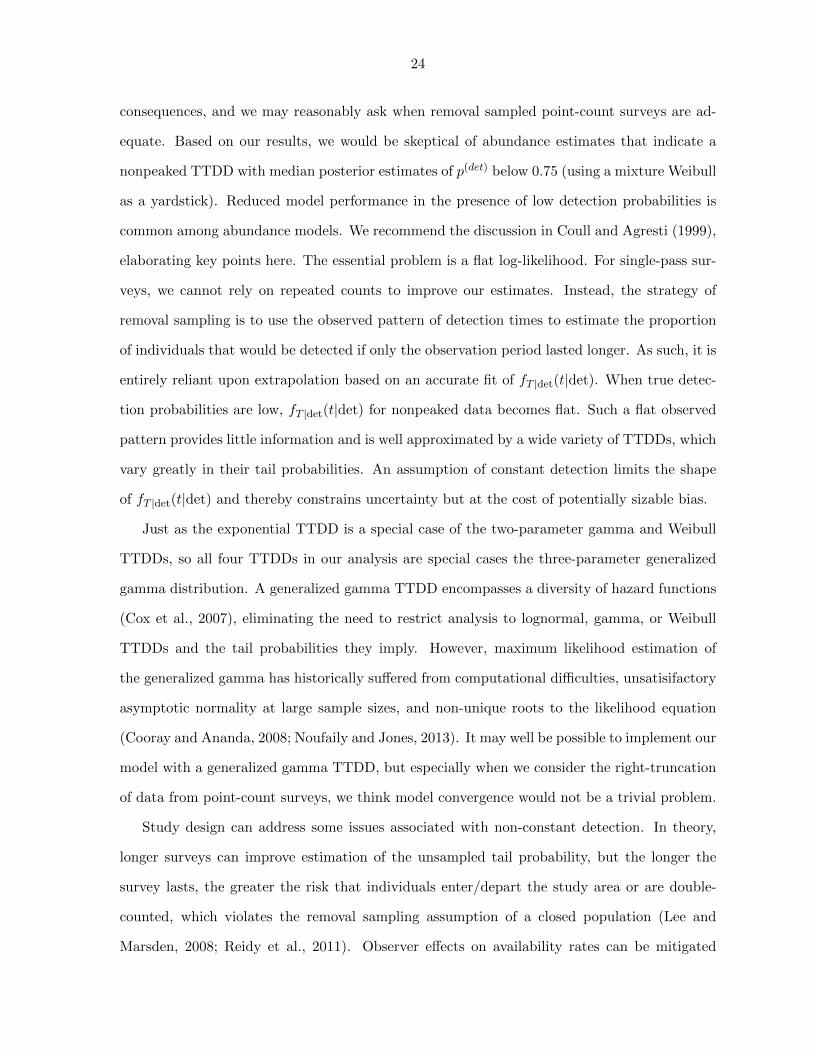
3.3 Model comparisons of event and state models using expected predictive
accuracy (∆elpd) . . . . . . . . . . . . . . . . . . . . . . . . . . . . . . 44
4.1 Schematic of designs featuring 4-8 meter prairie strips spaced at dis-
tances of 40 meters in rowcrop-planted fields . . . . . . . . . . . . . . . 51
4.2 Density of counts by species as a function of distance (i.e., counts scaled
by distance) . . . . . . . . . . . . . . . . . . . . . . . . . . . . . . . . . 55

vii
4.3 Total detections by time interval for each species plus empirical density
plots of observed distances by time interval for all species . . . . . . . 56
4.4 Posterior estimates of abundance density marginally across all surveys
for models fit with varying truncation distances . . . . . . . . . . . . . 57
4.5 Posterior estimates for each species of: (i) expected log-scale abundance
per survey by treatment-year, and (ii) pairwise comparisons among
treatments . . . . . . . . . . . . . . . . . . . . . . . . . . . . . . . . . . 58
4.6 Posterior marginal estimates of abundance density (per km2), detection
probability, availability, and perceptibility for each species . . . . . . . 59
4.7 Posterior availability and perceptibility estimates for all species . . . . 60
A.1 Posterior estimates of p(det) across TTDD families from Section 2.4.3 . 78
A.2 Posterior parameter estimates for all models fit to the simulated non-
mixture exponential dataset in Section 2.4.3 . . . . . . . . . . . . . . . 79
A.3 Posterior parameter estimates for all models fit to the simulated expo-
nential mixture dataset in Section 2.4.3 . . . . . . . . . . . . . . . . . . 80
A.4 Posterior parameter estimates for all models fit to the simulated non-
peaked non-mixture gamma dataset in Section 2.4.3 . . . . . . . . . . . 81
A.5 Posterior parameter estimates for all models fit to the simulated non-
peaked gamma mixture dataset in Section 2.4.3 . . . . . . . . . . . . . 82
A.6 Posterior parameter estimates for all models fit to the simulated peaked
non-mixture gamma dataset in Section 2.4.3 . . . . . . . . . . . . . . . 83
A.7 Posterior parameter estimates for all models fit to the simulated peaked
gamma mixture dataset in Section 2.4.3 . . . . . . . . . . . . . . . . . 84
A.8 Posterior parameter estimates for all models fit to the simulated non-
peaked non-mixture lognormal dataset in Section 2.4.3 . . . . . . . . . 85
A.9 Posterior parameter estimates for all models fit to the simulated non-
peaked lognormal mixture dataset in Section 2.4.3 . . . . . . . . . . . . 86
viii
A.10 Posterior parameter estimates for all models fit to the simulated peaked
non-mixture lognormal dataset in Section 2.4.3 . . . . . . . . . . . . . 87
A.11 Posterior parameter estimates for all models fit to the simulated peaked
lognormal mixture dataset in Section 2.4.3 . . . . . . . . . . . . . . . . 88
A.12 Posterior parameter estimates for all models fit to the simulated non-
peaked non-mixture Weibull dataset in Section 2.4.3 . . . . . . . . . . 89
A.13 Posterior parameter estimates for all models fit to the simulated non-
peaked Weibull mixture dataset in Section 2.4.3 . . . . . . . . . . . . . 90
A.14 Posterior parameter estimates for all models fit to the simulated peaked
non-mixture Weibull dataset in Section 2.4.3 . . . . . . . . . . . . . . . 91
A.15 Posterior parameter estimates for all models fit to the simulated peaked
Weibull mixture dataset in Section 2.4.3 . . . . . . . . . . . . . . . . . 92
B.1 Posterior estimates of detection probability p(det) from a representative
complete replicate set of simulations . . . . . . . . . . . . . . . . . . . 114
B.2 Posterior estimates for availability pa from a representative complete
replicate of simulations for event, state, and combined models fit to
event and state data at various levels of availability and perceptibility 116
B.3 Posterior estimates for perceptibility from a representative complete
replicate of simulations for event, state, and combined models fit to
event and state data at various levels of availability and perceptibility 117
B.4 Model comparisons between combined and true models in expected pre-
dictive accuracy (∆elpd) . . . . . . . . . . . . . . . . . . . . . . . . . . 118
C.1 Posterior marginal estimates of abundance density (per km2), detec-
tion probability, availability, and perceptibility for each species at every
truncation distance. . . . . . . . . . . . . . . . . . . . . . . . . . . . . . 120
C.2 All posterior parameter estimates at all truncation distances for Amer-
ican robins. . . . . . . . . . . . . . . . . . . . . . . . . . . . . . . . . . 121

ix
C.3 All posterior parameter estimates at all truncation distances for common
yellowthroat. . . . . . . . . . . . . . . . . . . . . . . . . . . . . . . . . . 122
C.4 All posterior parameter estimates at all truncation distances for dickcissels.123
C.5 All posterior parameter estimates at all truncation distances for eastern
meadowlarks. . . . . . . . . . . . . . . . . . . . . . . . . . . . . . . . . 124
C.6 All posterior parameter estimates at all truncation distances for killdeer. 125
C.7 All posterior parameter estimates at all truncation distances for red-
winged blackbirds. . . . . . . . . . . . . . . . . . . . . . . . . . . . . . 126

x
ACKNOWLEDGEMENTS
Since my first year in Snedecor Hall, I have felt I am among my people. I grok the way
statisticians interact with and make sense of the world. I owe thanks and much of my sense
of belonging to the Department of Statistics, its faculty and staff. The Department hosts an
uncommonly communal academic culture. I feel respected and valued, and I sense clearly the
Department’s desire for me to succeed. To a person, I have found the faculty helpful and
accessible.
I wish to thank Jess Severe, who has been indispensible in navigating all things administra-
tive. I owe thanks to the statistical consulting group. Not only has consulting helped pay for my
studies, but it has imbued me with a science-oriented context for statistics, which is downright
fundamental to my understanding and practice of the discipline. I am grateful to many in my
cohort of graduate students, who love nothing better than to brainstorm and debate answers
to homework problems. Two fellow students have been indispensible. Many, many thanks to
Lendie Follett, boon consulting companion and strangely kindred spirit. Many, many thanks
to Gabriel Demuth – nearly every good idea in this dissertation has been refined and tempered
in cross-campus discussions; there are days I feel I have learned as much in dialogue with Gabe
as through my coursework.
I offer thanks to Dr. Gerald Niemi and the Natural Resources Research Institute for sharing
point-count survey data from the Minnesota Forest Breeding Bird Survey. These data are, in
a real sense, the source of my dissertation. Thanks likewise go to Dr. Lisa Schulte Moore and
the STRIPs project for sharing point-count distance-removal data with which to appraise my
distance-removal model.
I have been fortunate with my duo of co-advisors, who have diligently, patiently propelled
me along the multi-dimensional path that is modern-day statistics. To Philip, I am most

xi
grateful for your sense of perspective, which orients my sense of proportion and which ways are
forward and up. To Jarad, I am grateful for your ceaseless energy and high standards. If ever
somebody praises me on the cleanliness of my code or the organization of my file directories,
the credit should transmit to you.
Lastly and most importantly, my love and deepest gratitude go to my wife Angie and
daughter Clare. The daily sacrifices of family before the altar of graduate school are understood
by those who have endured it. There is nothing I more eagerly anticipate than the return of
time with my family.

xii
ABSTRACT
In this disseration, we estimate abundance from removal-sampled animal wildlife point-
count surveys, focusing on models to account for heterogeneous detection probabilities. In con-
trast to many published models, our research treats individual times to detection as continuous-
time responses. Adopting this method enables us to ask questions that are impractical under
existing discrete-time models. We accomplish our analyses by using a parametric survival
analysis approach within the N-mixture class of hierarchical animal abundance models. In
Chapter 2, we construct models for removal-sampled data that allow detection rates to change
systematically over the course of each observation period. Most studies assume detection rates
are constant, but our analysis demonstrates this assumption to be very informative, leading
to biased and overly precise estimates. Non-constant models prove less biased with better
coverage statistics over a range of simulated datasets. In Chapter 3, we extend the continuous-
time modeling approach to distance-removal sampled surveys. We introduce a new model that
successfully integrates two subtly different existing mechanisms for modeling distance-removal
surveys: one that focuses on detecting available individuals and one that focuses on detecting
availability cues (e.g. bird calls). We articulate the distinctions between the two and place
them with current terminology for availability and perceptibility. Our new model accurately
estimates abundance and detection from datasets simulated via either mechanism, but models
that assume only one mechanism are often not robust to misspecification. In Chapter 4, we ap-
ply our model from Chapter 3 to six avian species monitored in removal- and distance-sampled
point-count surveys in Iowa agricultural fields. We articulate several ways in which the model
does not match data characteristics, and we identify priorities for developing this model in
order to make it more flexible and feasible.

1
CHAPTER 1. INTRODUCTION
Statistical models for wildlife surveys must account for variations in detection probability
across individual site surveys in order to generate reliable estimates of species abundance (Pol-
lock et al., 2002; Nichols et al., 2009). To estimate detection probabilities, we decompose the
process of detection into two stages: an animal must make itself available to be detected by
producing a detectable cue (e.g. a movement or an audible call), and an observer conduct-
ing the study must perceive the available animal (Farnsworth et al., 2002; McCallum et al.,
2005; Nichols et al., 2009). Two methods that have proven useful in estimating these stages
separately are point-count removal sampling (Farnsworth et al., 2002) and distance sampling
(Buckland et al., 2001). Point-count removal sampled data contain times to first detection for
each observed animal. The pattern of these detection times provides information about how
often animals produce detectable cues. Distance sampled data contain distances from the ob-
server for each observed animal. The pattern of detection distances provides information about
the observer’s ability to perceive cues and also allows abundance estimation per unit area.
In this dissertation, we examine the statistical analysis of single-visit removal-sampled and
distance-removal-sampled point-count surveys. The statistical idea that motivates our work
is that removal-sampled times to detection should be modeled as continuous responses rather
than discrete, as is often done. This idea invites a parametric survival analysis approach, which
in turn facilitates our ability to ask new questions and formulate new models.
1.1 Point-count survey datasets
The models we present in this dissertation analyze single-species data from removal-sampled
and removal-distance-sampled single-visit avian point-count surveys. We draw upon two multi-

2
species datasets: the Minnesota Forest Breeding Bird Project (MNFB) (Hanowski et al., 1995)
and the Science-based Trials of Rowcrops Integrated with Prairie Strips (STRIPs) at Iowa State
University. The MNFB dataset features 381 ten-minute survey periods conducted by trained
observers during which the first detection time for each bird is censored into nine intervals. This
relatively fine scale of interval-censoring is atypical for removal-sampled datasets but proves
invaluable for our purpose of estimating time-varying detection rates. The dataset also contains
coarsely interval-censored distances, which we do not use in our analyses. The STRIPs dataset
features 511 five-minute survey periods all conducted by the same observer. Detection times are
censored into five intervals, and distances are measured to the nearest meter with a laser range
finder. The possession of exact distances proves to be a computational advantage in applying
distance-removal models. Both datasets contain records about survey sites (e.g. habitat) and
observation conditions (e.g. time of day, wind conditions) which we use as covariates in our
models.
1.2 Continuous-time removal-only models
Historically, removal models assume both discrete time responses and constant rates of
detection (Moran, 1951; Seber, 1982; Farnsworth et al., 2002; Royle, 2004a). In our opinion,
these two assumptions have been mutually reinforcing. Observers typically censor detections
according to predetermined intervals, which may vary in length (Ralph et al., 1995). A standard
analysis subdivides the survey period into equal-duration intervals. For any individual animal
at a given survey, the probability of detection during any interval (given that it has not already
been detected) is assumed to be constant. However, there are many reasons to believe that
detection rates are not constant during point-count surveys (Alldredge et al., 2007a; Lee and
Marsden, 2008). Indeed, avian point-count surveys frequently exhibit elevated counts during the
first interval. Some models adopt an ad hoc approach to this pattern by specifying a separate
detection probability for just the first interval (Farnsworth et al., 2002; Efford and Dawson,
2009; Etterson et al., 2009), but this approach does not change the underlying assumption that
detection rates are constant across the remaining survey intervals.
We approach removal-sampled detection times as fundamentally continuous responses

3
(Solymos et al., 2013; Borchers and Cox, 2016) that follow a time-to-detection distribution
(TTDD). When observation protocols dictate interval-censored record-keeping, we can still
calculate interval-specific detection probabilities by integrating the TTDD accordingly, but the
very act of doing so encourages us to contemplate a variety of forms for the TTDD. So, beyond
the constant-rate default exponential distribution, we postulate TTDDs that follow gamma,
lognormal, and Weibull distributions.
In turn, the consideration of non-constant TTDDs causes a heightened awareness of the
roles that right-truncation and extrapolation play in removal analysis. Right-trunctation occurs
because animals not detected during the observation window are never detected and therefore
not known to exist. Indeed, this is the central question in removal sampling: how many
animals were never detected? Removal modeling addresses right-truncation by fitting a TTDD
to observed times and then extrapolating it into the unobserved period. The quality of that
extrapolation depends upon both: (i) how well the TTDD matches the observed pattern of the
data, and (ii) how well the TTDD matches the pattern of the ‘unobserved data’.
The modeling of non-constant detection rates in removal-only abundance estimation, and
our ability to fit TTDDs to both observed and unobserved detection times, is the subject matter
of Chapter 2.
1.3 Continuous-time distance-removal models
Unified modeling of removal- and distance-sampled data is a recent innovation (Farnsworth
et al., 2005; McCallum et al., 2005), and unified modeling within a hierarchical context that al-
lows for mixed effects is even more recent (Borchers et al., 2013; Solymos et al., 2013; Amundson
et al., 2014; Borchers and Cox, 2016). To some degree, the approaches implemented in these
models reflect their split heritage. On one side are removal-inspired models based largely on
avian point-counts. They model the joint distribution of observed times and distances as a
multinomial response, reflecting the interval-censoring often used in collection of both data
types. On the other side are distance-inspired models based largely on shipboard marine mam-
mal line transects. They model distance as continuous and treat time mainly as a proxy for
forward distance relative to the ship. The two model types likewise focus on different ranges

4
of animal behaviors and of habitats.
It is therefore unsurprising that the two model lineages differ in how they synthesize removal
and distance methods. In particular, with regard to an observer’s perception of animals in the
field, the two modeling approaches differ on the fundamental observational unit for percepti-
bility. Discrete-time models (Diefenbach et al., 2007; Solymos et al., 2013; Amundson et al.,
2014) functionally emphasize the perception of available animals. Continuous-time models —
including Borchers and Cox (2016) and extension of our own work from Chapter 2 — func-
tionally emphasize the perception of availability cues produced by animals. Neither modeling
approach is wrong, but they embody different assumptions and yield differing inference.
In Chapter 3, we detail the differences between these model types with regard to definitions,
assumptions, and mathematics. We use simulation studies to demonstrate the differences. We
then compose a combined hierarchical distance-removal model that successfully integrates both
the discrete- and continuous-time approaches. Like its antecedents, the combined model can
incorporate mixed effects for abundance, availability, and perceptibility of animals according
to site-level and survey-level covariates and effects.
In Chapter 4, we test drive our new combined distance-removal model using point-count
survey field data. We identify limitations of the model with respect to data issues, and we
build upon the experience to prioritize future developments of the model.

CHAPTER 2. ASSESSING THE IMPACTS OF TIME TO DETECTION
DISTRIBUTION ASSUMPTIONS ON DETECTION PROBABILITY
ESTIMATION
A paper submitted to the Journal of Agricultural, Biological, and Environmental Statistics
Adam Martin-Schwarze, Jarad Niemi, and Philip Dixon
Abstract
Abundance estimates from animal point-count surveys require accurate estimates of detec-
tion probabilities. The standard model for estimating detection from removal-sampled point-
count surveys assumes that organisms at a survey site are detected at a constant rate; however,
this assumption can often lead to biased estimates. We consider a class of N-mixture models
that allows for detection heterogeneity over time through a flexibly defined time-to-detection
distribution (TTDD) and allows for fixed and random effects for both abundance and detec-
tion. Our model is thus a combination of survival time-to-event analysis with unknown-N,
unknown-p abundance estimation. We specifically explore two-parameter families of TTDDs,
e.g. gamma, that can additionally include a mixture component to model increased probabil-
ity of detection in the initial observation period. Based on simulation analyses, we find that
modeling a TTDD by using a two-parameter family is necessary when data have a chance of
arising from a distribution of this nature. In addition, models with a mixture component can
outperform non-mixture models even when the truth is non-mixture. Finally, we analyze an
Ovenbird data set from the Chippewa National Forest using mixed effect models for both abun-
dance and detection. We demonstrate that the effects of explanatory variables on abundance
6

7
and detection are consistent across mixture TTDDs but that flexible TTDDs result in lower
estimated probabilities of detection and therefore higher estimates of abundance.
Keywords: abundance; availability; hierarchical model; Markov chain Monte Carlo; N-
mixture model; point counts; removal sampling; Stan; survival analysis

8
2.1 Introduction
Abundance estimates from animal point-count surveys require accurate estimates of detec-
tion probabilities. Removal sampling, where individuals are solely counted on their first capture,
provides one established methodology for estimating detection probabilities (Farnsworth et al.,
2002). A standard assumption in removal sampling is a constant detection rate throughout the
observation period, but this assumption is often unjustified (Alldredge et al., 2007a; Lee and
Marsden, 2008). In particular, animal behaviors such as intermittent singing in birds and frogs
or diving in whales (Scott et al., 2005; Diefenbach et al., 2007; Reidy et al., 2011), differences
in behavior across subgroups of animals (Otis et al., 1978; Farnsworth et al., 2002), observer
impacts on animal behaviors (McShea and Rappole, 1997; Rosenstock et al., 2002; Alldredge
et al., 2007a), and variations in observer effort, e.g. saturation or lack of settling down period
(Petit et al., 1995; Lee and Marsden, 2008; Johnson, 2008), can all lead to time-varying rates
of detection.
In this manuscript, we develop a model for scenarios where detection rates are not constant
over time. We analyze times to first detection as time-to-event data, as is done in parametric
survival analysis, defining a continuous random variable T for each individual’s time to first
detection with a probability density function (pdf) fT (t) and cumulative distribution function
(cdf) FT (t). We refer to the distribution of T as a time-to-detection distribution (TTDD).
One common strategy to deal with data that do not fit a constant-detection assumption is
to model the TTDD as a mixture of two distributions — a continuous-time distribution and
a point mass for increased detection probability in the initial observation period (Farnsworth
et al., 2002, 2005; Efford and Dawson, 2009; Etterson et al., 2009; Reidy et al., 2011). However,
this is not yet the standard (Solymos et al., 2013; Amundson et al., 2014; Reidy et al., 2016).
We consider the choice of whether to include a mixture component in conjunction with TTDDs
with non-constant rates and apply the term mixture TTDD when the TTDD has a discrete
and continuous component.
Unlike most survival analyses, the number of individuals N present at a survey is unknown
and may be the primary quantity of interest. We embed the TTDD in a hierarchical framework

9
for multinomial counts called an N-mixture model (Wyatt, 2002; Royle, 2004b), which is an
entirely different use of ‘mixture’ from the mixture models in the previous paragraph. For
our purposes, the N-mixture framework provides three clear benefits: 1) it handles counts
within a flexible multinomial data framework (Royle and Dorazio, 2006) which accords with
the interval-censored data collection that is customary in point-count surveys (Ralph et al.,
1995), 2) the hierarchical structure readily lends itself to including abundance- and detection-
related covariates and random effects (Dorazio et al., 2005; Etterson et al., 2009; Amundson
et al., 2014), and 3) for a Bayesian analysis, we can sample the posterior joint distribution
of N-mixture parameters straight-forwardly using Markov chain Monte Carlo (MCMC). The
N-mixture framework models abundance as a latent variable with a Poisson or other discrete
distribution and independently models detection probabilities. Several previous studies have
employed the N-mixture framework to analyze removal sampled point-count data (Royle, 2004a;
Dorazio et al., 2005; Etterson et al., 2009; Solymos et al., 2013; Amundson et al., 2014; Reidy
et al., 2016).
Framing a model in terms of time-to-detection leads to two practical differences vis-a-vis
constant-detection models. First, in order to model covariate and random effects on detection,
we perform mixed effects linear regression on the log of the rate parameter as in Solymos
et al. (2013), whereas most existing studies instead construct regression models on the logit
of the equal-interval detection probability. The latter is not possible when detection rates
are not constant. Second, because we can obtain interval-specific detection probabilities from
the TTDD by partitioning its cdf (Figure 2.1), we can directly model the data according to
their existing interval structure rather than subdividing the observation period into intervals of
equal duration. Indeed our model fits exact time-to-detection data, whereas existing constant-
detection removal models only approximate exact data by subdividing the observation interval
into a large number of fine equal-duration intervals (Reidy et al., 2011; Amundson et al., 2014).
Section 2.2 provides a description of the interval-censored time-to-detection avian point
count data under consideration. Section 2.3 introduces an N-mixture model with a generically
defined TTDD for estimating abundance from removal-sampled point-count surveys. Section
2.4 provides three simulation studies to assess the impact of TTDD choice on estimated detec-

10
tion probability. Section 2.5 analyzes an Ovenbird data set under different TTDDs to determine
the impact of this choice on estimated detection probability and therefore estimated abundance.
2.2 Interval-censored point counts
Our analysis is motivated by avian point-count surveys in Chippewa National Forest from
2008-2013 as part of the Minnesota Forest Breeding Bird Project (MNFB) (Hanowski et al.,
1995). For our analysis, we focus on Ovenbird counts selected from one habitat type: sawtimber
red pine stands with no recent logging activity. Each stand had up to four sites with sufficient
geographical distance between sites to reduce or eliminate overlapping territories. This dataset
includes 947 Ovenbirds counted in 381 surveys at 65 sites with site-specific variables including
site age, stock density, and an indicator of select-/partial-cut logging during the 1990s.
Single-visit (per year) point-count surveys were conducted by trained observers at each site
once annually (weather permitting). Fourteen different observers conducted surveys during
the study period and 69% of surveys in our dataset involved observers in their first year at
the MNFB. Survey durations were 10 minutes, with times to first detection censored into nine
intervals: a two-minute interval followed by eight one-minute intervals. During each survey,
the Julian date, time of day, and temperature were recorded.
While we focus on the estimation of detection probability in avian populations, the approach
we describe is appropriate for point-count surveys of any species. The methodology allows the
analysis of data with 1) recorded first (possible censored) detection of each individual, 2) site-
specific explanatory variables, and 3) survey-specific explanatory variables.
2.3 Continuous time-to-detection N-mixture models
Before considering interval censoring and explanatory variables, we first present the sce-
nario of exact times to detections with no explanatory variables. We then incorporate interval
censoring and follow with inclusion of fixed and random effects for abundance and detection.

11
Time
Den
sity
0 C
p(det) = 0.71
1−p(det)
Cou
nts
per
Min
ute
Time0 2 3 4 5 6 7 8 9 10
05
1015
2025
3035
Time
Den
sity
0 C
p(det) = 0.94
1 − γ
Figure 2.1 Illustration of fitting mixture exponential (left) and mixture gamma (right) time–to-detection distributions (TTDDs) to interval-censored removal-sampled observa-tions (center). The mixture TTDD consists of a continuous TTDD (thick line)plus a mixture component of first-interval detections (light gray rectangle), consti-tuting γ and 1− γ proportions of the population, respectively. We estimate p(det)
as the proportion of the TTDD before the end of the observation period C, leavingan estimated proportion 1− p(det) undetected.
2.3.1 Distributions for exact times to detection
Suppose that, for each survey s (s = 1, . . . , S), Ns individuals are present. Imagine an ob-
server could remain at the survey location until every individual is detected, recording the time
to detection tsb (for bird, b = 1, . . . , Ns) for each. Assuming detection times for all individuals
at a survey are independent, identically distributed according to a common time-to-detection
distribution (TTDD), we define Tsb as a random variable with cumulative distribution function
(cdf) FT (t) and probability density function (pdf) fT (t). In practice, times to first detection
are truncated due to a finite survey length of C, meaning each individual has detection prob-
ability p(det) = FT (C). The conditional distribution of observed detection times consequently
has pdf fT |det(t|det) = fT (t)/FT (C) for 0 < t < C, cdf FT |det(t|det) =∫ t0 fT |det(x|det)dx, and
instantaneous detection rate, or hazard function, h(t) = fT (t)/[1− FT (t)].
A common choice for TTDD is an exponential distribution, i.e. Tsbind∼ Exp(ϕ), which
imposes a constant first detection rate, i.e. h(t) = ϕ. By choosing another TTDD, we can allow
for a systematic non-constant detection regime. For example, to model an observer effect where:
(i) the observer’s arrival suppresses or stimulates detectable cues, but (ii) individuals acclimate

12
and gradually return to constant detection, a gamma TTDD would be appropriate. Like the
gamma TTDD, Weibull and lognormal TTDDs offer the flexibility of a two-parameter form and
allow rates to increase or decrease during the survey. All three TTDDs may provide reasonable
empirical approximations of non-constant detection, though the shapes of the distributions
differ, potentially leading to differing inference. For instance, when detection rates vary across
individuals, the result is a marginal detection rate that decreases over time. Whether the
marginal rate is best approximated by a gamma, lognormal, Weibull, or some other TTDD
depends on just how rates vary across individuals.
To facilitate the later inclusion of fixed and random effects, we use the following rate-based
parameterizations: T ∼ Exp(ϕ), E[T ] = 1/ϕ; T ∼ Ga(α,ϕ), E[T ] = α/ϕ; T ∼ We(α,ϕ),
E[T ] = Γ(1 + 1/α)/ϕ; and T ∼ LN(ϕ, α), E[T ] = exp(α2/2)/ϕ. This parameterization of the
lognormal relates to the standard (µ, σ2) parameterization by ϕ = exp(−µ) and α = σ. The
exponential distribution is a special case of both the gamma and Weibull distributions when
α = 1. We employ a log link to model ϕ, and therefore our model is equivalent to a generalized
linear model with a log link on the mean detection time.
2.3.2 TTDDs in an N-mixture model
A basic N-mixture model describes observed survey-level abundance n(obs) with a hier-
archy where n(obs)s
ind∼ Binomial(Ns, p
(det))
and Nsind∼ Po(λ). We can decompose Ns into
observed and unobserved portions: n(obs)ind∼ Po(λp(det)) and, independently, n
(unobs)s
ind∼
Po(λ[1− p(det)]
). Although alternative distributions can be considered, e.g. negative bino-
mial, our experience with Ovenbird point counts suggests that, after accounting for appro-
priate explanatory variables, the resulting abundances are likely underdispersed rather than
overdispersed, and thus we will use the Poisson assumption here.
The above definitions complete our exact-time homogenous-survey data model, consisting

13
of distributions for counts and observed detection times:
n(obs)sind∼ Po(λp(det))
p(ts) =∏
b=1...n(obs)s
fT |det(tsb| det, α, ϕ) (2.1)
p(det) = FT (C|α,ϕ)
where ts is a vector of observed times at survey s.
2.3.3 Interval-censored times to detection
Due to the harried process of avian point counts, times to first detection are typically not
recorded exactly, but are instead censored into I intervals. Let Ci for i = 1, . . . , I indicate the
right endpoint of the ith interval then CI is the total survey duration and, letting C0 = 0,
the ith interval is (Ci−1, Ci]. Let nsi be the number of individuals counted during interval
i on survey s, n(obs)s =
∑Ii=1 nsi, and ns = (ns1, . . . , nsI). Assuming independence amongst
individuals and sites, we have nsind∼ Mult
(n(obs)s ,ps
), where ps = (ps1, . . . , psI) and psi =
FT |det(Ci|det)− FT |det(Ci−1|det) =∫ Ci
Ci−1fT |det(t)dt, see Figure 2.1.
2.3.4 Detection heterogeneity across subgroups
It is common in avian point counts to observe increased detections in the first interval
relative to an exponential distribution. This is often understood to reflect unmodeled detection
heterogeneity across behavioral groups in the study population. Failure to account for such
heterogeneity in the constant-detection scenario leads to negative bias in abundance estimates
(Otis et al., 1978). To accommodate this empirical observation, many models of interval-
censored removal times define a TTDD with a mixture component to increase the probability
of observing individuals in the first interval (Farnsworth et al., 2002; Royle, 2004a; Farnsworth
et al., 2005; Alldredge et al., 2007a; Etterson et al., 2009; Reidy et al., 2011). We specify a
mixture TTDD with mixing parameter γ ∈ [0, 1], a point-mass during the first observation
interval, and a continuous-time detection distribution F(C)T (t). The mixture TTDD cdf is
defined: FT (t) = (1− γ) + γF(C)T (t) for t > 0. If γ = 1, the non-mixture model is recovered.

14
2.3.5 Incorporating explanatory variables
As discussed in Section 2.2, explanatory variables are available for sites and for surveys.
Generally, we suspect that site variables, e.g. habitat, will affect abundance and survey vari-
ables, e.g. time of day, will affect detection probability. Thus, we allow for incorporating
explanatory variables on both the abundance and detection.
To incorporate explanatory variables on abundance, we model the expected survey abun-
dance λs with log-linear mixed effects, i.e. log(λs) = XAs β
A+ZAs ξA where XA
s are explanatory
variables, βA is a vector of fixed effects, ZAs specifies random effect levels, and ξAjind∼ N(0, σ2A[j])
are random effects where A[j] assigns the appropriate variance for the jth abundance random
effect.
To incorporate explanatory variables on detection probability, we let the continuous portion
of the TTDD depend on the explanatory variables through the now site-specific parameter ϕs.
Specifically, we model log(ϕs) = XDs β
D + ZDs ξD, where XD
s are explanatory variables, βD is a
vector of fixed effects, ZDs specifies random effect levels, ξDjind∼ N(0, σ2D[j]) are random effects
where D[j] assigns the appropriate variance for the jth detection random effect. For simplicity,
we assume the shape parameter α as constant across sites.
2.3.6 Estimation
For ease of reference, the final full model is provided in Equation (2.2) where the conditioning
of the TTDD cdf on α and ϕs is made explicit.
n(obs)sind∼ Po(λsp
(det)s )
nsind∼ Mult(n(obs)s ,ps); ps = (ps1, . . . , psI)
p(det)s = FT (CI |α,ϕs)
ps1 =[(1− γ) + γF
(C)T (C1|α,ϕs)
]/p(det)s (2.2)
psi = γ[F
(C)T (Ci|α,ϕs)− F (C)
T (Ci−1|α,ϕs)]/p(det)s
log(λs) = XAs β
A + ZAs ξA; ξAj
ind∼ N(0, σ2A[j])
log(ϕs) = XDs β
D + ZDs ξD; ξDj
ind∼ N(0, σ2D[j])
15
We adopt a Bayesian approach and therefore require a prior over the model parameters. To
ease construction of a default prior for this model, we standardize all explanatory variables and
then construct priors to be diffuse within a reasonable range of values. Normal prior mean and
standard deviation (sd) for the abundance intercept was set at a median abundance of 3 birds
per site and a 95% probability of 0-14 birds present (counted and uncounted). Normal prior
mean and sd for the detection intercept were chosen so that, based on an intercept-only non-
mixture model with α = 1: (i) median prior detection probability was p(det)s = 0.50, and (ii)
95% of the prior detection probability was within p(det)s ∈ (0.01, 1.0). Normal priors for fixed
effect parameters were centered at zero with standard deviations matching the appropriate
intercept term. All standard deviations and α were given half-Cauchy priors with location 0
and scale 1 for the untruncated Cauchy, and the mixture parameter γ was assigned a Unif(0,1)
prior in mixture models. All scalar parameters were assumed independent a priori.
We fit the models by MCMC sampling using the Bayesian statistical software Stan, imple-
mented via the R package rstan version 2.8.0 (Stan Development Team, 2016). We discarded
half of the iterations as warmup and thinned by 10. We monitored convergence of the MCMC
chains using Geweke z-score diagnostics (Geweke et al., 1991) and reran models if lack of con-
vergence was indicated by a non-normal distribution of the z-scores or if the effective sample
size for any parameter was below 1000. The number of iterations used depended on the model
and is detailed later. For most models, we accepted Stan defaults for initial values; however,
gamma and Weibull models sometimes failed to run unless care was taken in the specification
of initial values.
2.4 Simulation studies
We conducted three simulation studies to explore the behavior of models with non-constant
TTDDs. The first study compares mixture vs non-mixture models. The second study compares
the TTDD families. In the first two studies, we utilized intercept only models to focus attention
on robustness of the TTDD choice in the most simple of scenarios. For the third study, we
included fixed and random effects for both abundance and detection and again compared the
distribution families. In all simulation studies, we focused on accuracy in estimation of p(det)

16
which then translated into estimation of abundance.
In the following analyses we distinguish two categories of purely continuous TTDDs: peaked
and nonpeaked. Detection rates h(t) of peaked distributions generally increase over time, while
detection rates of nonpeaked distributions generally decrease over time. More formally, we
define a peaked TTDD as having a mode greater than zero (or C1 for lognormal) while a
nonpeaked TTDD has a mode of zero (or less than C1), but we consider exponential TTDDs
to be neither peaked nor nonpeaked.
2.4.1 Mixture versus non-mixture TTDDs
To assess the need for incorporating a mixture component to increase the probability of
detection in the initial interval as discussed in Section 2.3.3, we simulated 5600 intercept-only
datasets: 100 replicates using 4 values of p(det) (0.50, 0.65, 0.80, and 0.95) from each of 14
TTDDs (each combination of peaked/nonpeaked, mixture/non-mixture, and exponential/gam-
ma/Weibull/lognormal, where exponential models are considered nonpeaked). We chose true
parameter values (Table A.1) and the number of surveys (381) to mimic the Ovenbird analysis
(Section 2.5). In particular, we set parameters such that (i) in nonpeaked models, 70% of
detected individuals were observed during the first two minutes, and (ii) in peaked models, the
detection mode for ‘hard to detect’ individuals occured at 5 minutes.
We fit each dataset with two models: mixture and non-mixture versions of the distribution
family, e.g. exponential, used to simulate the data. For each dataset-analysis combination, we
sampled > 90,000 iterations which showed no evidence of lack of convergence according to the
Geweke diagnostic and reached over 1,000 effective samples for all parameters.
For each dataset and inference model combination, we summarize the analysis across sim-
ulations by averaging the posterior median and reporting coverage for 90% credible intervals.
If analyses are providing reasonable estimates of p(det), we expect the average median to be
unbiased and the coverage to be close to 90%. Figure 2.2 provides a summary of these quanti-
ties. When a mixture model is used to simulate the data (lower row of plots), there is clearly
a benefit to using a mixture model for inference. Using a non-mixture model for inference,
the credible interval coverage is near zero for most models with the exponential model overes-
17
Nonpeaked Exponential Peaked
● ●●
●
● ●●
●
● ●●
●
● ●●
●
●
●
●
●
●
●
●
●
● ● ●
●
●●
●
●
0.2
0.4
0.6
0.8
1.0
0.2
0.4
0.6
0.8
1.0
Non−
Mixed
Mixed
50 65 80 95 50 65 80 95 50 65 80 95Actual Detection Probability
Est
imat
ed D
etec
tion
Pro
babi
lity
Nonpeaked Exponential Peaked
● ●● ●
●
● ●●
● ●
●
●
●● ●
●
● ● ● ●● ●● ●
● ● ● ●
● ●
● ●
0.0
0.5
1.0
0.0
0.5
1.0
Non−
Mixed
Mixed
50 65 80 95 50 65 80 95 50 65 80 95Actual Detection Probability
Cov
erag
e
Inference Model● ●
Non−mix Exponential
Non−mix Gamma
Non−mix Lognormal
Non−mix Weibull
Mix Exponential
Mix Gamma
Mix Lognormal
Mix Weibull
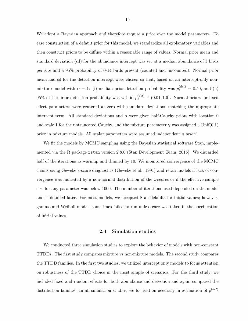
Figure 2.2 Comparisons of mixture and non-mixture TTDDs. Left : Average posterior me-dian detection probabilities across 100 replicate simulations. Dashed lines showunbiased estimation. Right : Coverage of 90% credible intervals across 100 repli-cate simulations. Dashed lines depict a 95% range of observed coverage that isconsistent with nominal coverage. Rows: Data simulated from non-mixture (up-per) or mixture (lower) TTDDs. Columns: Data simulated from nonpeaked (left),exponential (center), or peaked (right) TTDDs. Each inference model was fit onlyto datasets from the same TTDD family (e.g. lognormal to lognormal).
timating p(det) and the other models underestimating. When a non-mixture model is used to
simulate the data (upper row of plots), there are no clearly discernable differences between the
ability of a non-mixture or mixture model to capture p(det). These results support the general
default use of a mixture model over a non-mixture model.
For nonpeaked datasets, estimates of p(det) from the same TTDD inference model differed by
only 1-5% between p(det) = 0.50 and p(det) = 0.65 simulations (Tables A.3 to A.6), and credible
intervals had roughly the same widths. This suggests that, when data are nonpeaked with true
detection probabilities less than 65-80%, the patterns of detections over time are insufficient
for distinguishing between moderate and low values of p(det). In these cases, mixture inference
models estimated higher detection probabilities than did non-mixture models.

18
Nonpeaked Exponential Peaked
0.0
2.5
5.0
7.5
10.0
0.0
2.5
5.0
7.5
0.0
2.5
5.0
7.5
10.0
0
10
20
pdet = 0.5
pdet = 0.65
pdet = 0.8
pdet = 0.95
0.0 0.5 1.0 0.0 0.5 1.0 0.0 0.5 1.0Posterior Detection Probability
Den
sity
Nonpeaked Exponential Peaked
0
2
4
6
0
2
4
6
0
2
4
6
8
0
3
6
9
12
pdet = 0.5
pdet = 0.65
pdet = 0.8
pdet = 0.95
1.0 1.5 2.0 2.5 1.0 1.5 2.0 2.5 1.0 1.5 2.0 2.5Posterior log(Abundance) per Survey
Den
sity
Inference Model Family: Exponential Gamma
Figure 2.3 Representative examples of posterior distributions for p(det) (left panel) and sur-vey-level log-scale abundance (right panel). Data are simulated from nonpeakedgamma (left column), exponential (center), and peaked gamma (right) mixtureTTDDs. True detection probabilities vary by row and are shown for comparison(dashed vertical line). Inference models are either exponential mixture (light gray)or gamma mixture (dark gray) TTDDs.
2.4.2 Constant vs. non-constant detection mixture TTDDs
The previous section addressed model mis-specification in terms of the mixture component.
Now we turn to model misspecification of the distribution family. We simulated 100 replicates
of intercept-only datasets from the 7 different mixture TTDD models using the same detection
probabilties and parameters as in the previous section, and we fit them with mixture models
from each of exponential, gamma, lognormal, and Weibull families.
Figure 2.3 illustrates representative examples of posterior distributions for p(det) and site-
level log(abundance) when data and models were from the exponential and gamma mixture
TTDDs. Posterior distributions under exponential inference models accurately captured true
detection probabilities when the simulation model was exponential, but they overestimated (un-
derestimated) detection probabilities when the simulation model was nonpeaked (peaked). In
contrast, gamma family posteriors, which have added flexibility from having a shape parameter,
accurately captured the truth in most scenarios although with increased uncertainty.

19
Nonpeaked Peaked
●●
●
●
● ● ●
●
● ●●
●
● ● ●●
●●
●
●
●●
●●
● ●●
●
0.40.60.81.0
0.40.60.81.0
0.40.60.81.0
0.40.60.81.0
Exponential
Gam
ma
Lognormal
Weibull
50 65 80 95 50 65 80 95Actual Detection Probability
Est
imat
ed D
etec
tion
Pro
babi
lity
Nonpeaked Peaked● ●
●●
●● ●
●
●● ●
●
●● ●
●
● ●● ●
● ●
● ●
●●
●●
0.0
0.5
1.0
0.0
0.5
1.0
0.0
0.5
1.0
0.0
0.5
1.0
Exponential
Gam
ma
Lognormal
Weibull
50 65 80 95 50 65 80 95Actual Detection Probability
Cov
erag
e
Inference Model ●Exponential Gamma Lognormal Weibull
Figure 2.4 Comparisons of TTDDs across families. Left : Average posterior median detec-tion probabilities across 100 replicate simulations. Dashed lines show unbiasedestimation. Right : Coverage of 90% credible intervals across 100 replicate simu-lations. Dashed lines depict a 95% range of observed coverage that is consistentwith nominal coverage. Rows: Data simulated from mixture exponential, gamma,lognormal, or Weibull TTDDs. Columns: Data simulated from nonpeaked or ex-ponential (left) or peaked (right) TTDDs. All data and inference models usedmixture TTDDs.
Figure 2.4 and Tables A.7 to A.10 summarize posterior estimates of p(det) and coverage from
90% credible intervals across all TTDD families. The poorest estimation of p(det) occurred for
the exponential inferential model when the data simulation model had a peak, because the two
parameters (rate and mixing parameter) did not provide enough flexibility to adequately fit a
TTDD with both an initial increase and a delayed mode. As a result, the exponential model
underestimated the actual detection probability. In contrast, the exponential model typically
overestimated detection probability for nonpeaked simulated data. However, exponential model
estimates were both less biased and more precise when the data actually derived from an
exponential mechanism.
When comparing the different three-parameter TTDDs, model misspecification was not as
serious an issue because the models could better account for the patterns in time to detection.
Even so, estimates of p(det) amongst the three models differed by as much as 0.15. As in the
previous simulation study, estimates of p(det) from nonpeaked datasets changed little as true

20
values of p(det) decreased below 65-80%. For nonpeaked datasets, gamma TTDDs produced
larger estimates of p(det) than did Weibull TTDDs, with lognormal TTDDs producing the lowest
of all. For peaked datasets, the order of Weibull estimates were larger than gamma estimates.
Our results do not favor the use of one of these TTDDs over the others.
2.4.3 Models including covariates and random effects
The previous sections studied effects of time to detection assumptions in the context of
no explanatory variables. We now incorporate fixed and random effects for abundance and
detection to ascertain whether models differ in their estimates of effect sizes. We simulated
data from each of the 7 mixture TTDDs and fit models from exponential, gamma, lognormal,
and Weibull mixture models.
We simulated data using the median posterior parameter estimates obtained in the analysis
of Ovenbird data in Section 2.5. As those models differed in their estimates of p(det), so the
simulated datasets featured different true values of p(det). Because fitted Ovenbird models did
not yield peaked distributions, we simulated peaked data by: (i) using the same intercepts,
shape parameters, and mixing parameters as for peaked data (p(det) = 0.80) in previous simu-
lations, (ii) using median covariate and random effects from the Ovenbird estimates, and (iii)
scaling the detection intercept and random effect to achieve true detection probabilities ≈ 0.8
with a detection mode at 5 minutes. See Table A.2 for actual parameter values. Because of
the difficulty in integrating random effects over all sites, approximate posterior distributions
for the study-wide marginal p(det) were obtained by simulating data from each MCMC sample
and calculating the proportion of simulated Ovenbirds that were observed.
Computation times for this simulation study were much greater than for the other studies
because partitions of the cdf, e.g. F(C)T (Ci|α,ϕs), had to be calculated separately for every
survey; also, sampling often required 2-8 as many iterations. Average times for exponential,
lognormal, Weibull, and gamma model fits were 2.6, 5.1, 5.3, and 25+ hours, respectively, as
compared to only 2.0, 3.0, 3.3, and 5.3 minutes for the intercept-only models. Due to the
computation times involved, we fit each model only once.
The results from this simulation are qualitatively similar to the Ovenbird analysis (Figure

21
2.5) and thus we only briefly review the results here and provide the corresponding figures and
tables in Appendix A. Patterns in posterior estimates of overall detection probabilities with
respect to family TTDD forms were largely the same as in the previous simulation studies for
appropriate values of p(det) – the inclusion of explanatory variables did not make models more
robust to violations of constant-detection assumptions (Figure A.1). Posteriors for abundance-
related fixed and random effects were the same regardless of which TTDD was assumed (Ap-
pendix ?? and figures therein). Posteriors for the mixing parameter γ and detection-related
fixed and random effects were the same across gamma, lognormal, and Weibull mixture models
but were narrower and location-shifted for the exponential mixture model.
2.5 Ovenbird analysis
We fit the Ovenbird dataset with exponential, gamma, lognormal, and Weibull mixture
models. For the abundance half of our model, we used four covariates plus two random effects.
The covariates were: (a) site age, (b) survey year, (c) an indicator of whether the site stock
density was over 70%, and (d) an indicator of whether the site experienced select-/partial-cut
logging during the 1990s. We associated random effects with each survey year and each stand.
For the detection half of our model, we used covariates for: (a) Julian date, (b) time of day,
(c) temperature, (d) an indicator of whether it is the observer’s first year in the database,
and (e) an interaction between (a) and (d) to approximate a new observer’s learning curve.
We associated random effects with each observer. Preliminary model fits did not support
the inclusion of quadratic terms for any detection covariates. We centered and standardized all
continuous covariates prior to fitting models. We ran chains 250,000-375,000 iterations; Geweke
diagnostics showed no indication of lack of fit, and effective sample sizes were over 1000 for all
parameters.
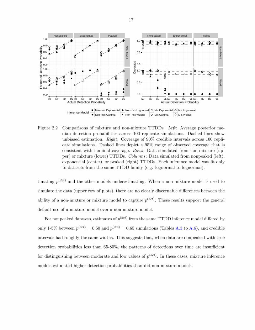
Figure 2.5 presents posterior medians and credible intervals for model parameters, overall
detection probability p(det), and the logarithm of total Ovenbird abundance. Estimates for the
shape parameter α from the gamma and Weibull models are consistent with the data arising
from an exponential distribution, although the uncertainty on this parameter remains relatively
large.

22
Abundance covariate coefficient estimates were virtually the same across all models. The
95% credible intervals for two of the abundance parameters (site age and logging) do not
contain zero, thereby suggesting notable effects. Select- and partial-cut logging events of the
1990s depressed local Ovenbird abundance during the study perior to roughly 25-50% of the
abundance for unlogged sites. Credible intervals for site age coefficient indicate that each decade
of age increases abundance from 1.5-13%. Credible intervals for detection parameters do not
indicate significant effects, after adjusting for the other predictors, for any of the included
predictors.
In spite of the similarity of effect parameter estimates, the posterior distributions for de-
tection probability and abundance differ greatly between the exponential and non-exponential
models. It is clear that the assumption of constant detection leads to much higher and more
precise estimates of detection than would be obtained if we are unwilling to make that assump-
tion.
2.6 Discussion
We formulated a model for single-species removal-sampled point-count survey data that
allows for non-constant detection rates. The model accommodates both interval-censored and
exact times to detection. Our model adopts a time-to-event approach within a hierarchical
N-mixture framework, and it allows times to first detection to be modeled according to flexibly
defined TTDD families. Our results show that non-constant TTDDs can return reasonable
estimates of detection probabilities across a variety of time-to-detection data patterns, whereas
traditional constant-rate TTDDs return biased and overly precise estimates when data deviate
from the constant-rate assumption, even when they include a mixture for heterogeneity across
groups. Because the exponential TTDD is a special case of both gamma and Weibull TTDDs,
we can interpret the differences in estimation between models as resulting from the information
conveyed by the assumption of constant detection.
We have additionally demonstrated for non-constant models the utility of using a mixture
TTDD formulation. Inference models with a mixture component are accurate under most
scenarios whether the data have a mixture or not, whereas inference models without the mixture
23
●
●
●
●
●
●
●
●
●
●
●
●
●
●
●
●
●
●
●
●
●
●
●
●
●
●
●
●
●
●
●
●
●
●
●
●
●
●
●
●
●
●
●
●
●
●
●
●
●
●
●
●
●
●
●
●
●
●
●
●
●
●
●
●
●
●
●
●
●
●
●
Intercept (A) Site Age (A) Year (A) Stock Density (A)
Logging (A) Year Std Dev (A) Stand Std Dev (A) Intercept (D)
Julian Date (D) Time of Day (D) Temperature (D) First Year (D)
JulDate x FirstYr (D) Observer Std Dev (D) γ α
p(det) log10(Abundance)
Lognormal MixWeibull Mix
Gamma MixExponential Mix
Lognormal MixWeibull Mix
Gamma MixExponential Mix
Lognormal MixWeibull Mix
Gamma MixExponential Mix
Lognormal MixWeibull Mix
Gamma MixExponential Mix
Lognormal MixWeibull Mix
Gamma MixExponential Mix
0.8 1.2 1.6 2.0 0.05 0.10 0.15 0.20 −0.2 −0.1 0.0 0.1 0.2 −0.2 0.0 0.2
−1.4 −1.2 −1.0 −0.8 0.0 0.1 0.2 0.3 0.4 0.50.00 0.05 0.10 0.15 0.20 −5 −4 −3 −2 −1
−0.4 −0.2 0.0 0.2 0.4 −0.4 −0.2 0.0 −0.25 0.00 0.25 −0.5 0.0 0.5 1.0
−0.50 −0.25 0.00 0.25 0.50 0.750.00 0.25 0.50 0.75 0.5 0.6 0.7 0.8 0.9 1.0 1 2 3
0.4 0.6 0.8 3.0 3.2 3.4
Posterior Parameter Estimates
Mod
el
Figure 2.5 Posterior medians (black dots) with 50% (wider line) and 95% (narrowerline) cred-ible intervals for the mixing parameter (γ), shape parameter (α) as well as abun-dance (A) and detection (D) fixed effects and random effect standard deviations.Posteriors are also available for the overall probability of detection and the abun-dance across all sites.
can be badly biased when the data do feature a mixture.
If the estimation of effect parameters and the roles of explanatory variables are the primary
interest, then our results suggest that the exact choice of TTDD may not be important. Abun-
dance effect estimates are similar regardless of the chosen TTDD. Detection effect estimates,
while conditional on the mixing parameter γ, are similar across all mixture non-exponential
TTDDs. These findings may well not hold if the same covariate is modeled in both abundance
and detection models (Kery, 2008).
If the estimation of abundance is the primary interest, then the choice of TTDD has large
24
consequences, and we may reasonably ask when removal sampled point-count surveys are ad-
equate. Based on our results, we would be skeptical of abundance estimates that indicate a
nonpeaked TTDD with median posterior estimates of p(det) below 0.75 (using a mixture Weibull
as a yardstick). Reduced model performance in the presence of low detection probabilities is
common among abundance models. We recommend the discussion in Coull and Agresti (1999),
elaborating key points here. The essential problem is a flat log-likelihood. For single-pass sur-
veys, we cannot rely on repeated counts to improve our estimates. Instead, the strategy of
removal sampling is to use the observed pattern of detection times to estimate the proportion
of individuals that would be detected if only the observation period lasted longer. As such, it is
entirely reliant upon extrapolation based on an accurate fit of fT |det(t|det). When true detec-
tion probabilities are low, fT |det(t|det) for nonpeaked data becomes flat. Such a flat observed
pattern provides little information and is well approximated by a wide variety of TTDDs, which
vary greatly in their tail probabilities. An assumption of constant detection limits the shape
of fT |det(t|det) and thereby constrains uncertainty but at the cost of potentially sizable bias.
Just as the exponential TTDD is a special case of the two-parameter gamma and Weibull
TTDDs, so all four TTDDs in our analysis are special cases the three-parameter generalized
gamma distribution. A generalized gamma TTDD encompasses a diversity of hazard functions
(Cox et al., 2007), eliminating the need to restrict analysis to lognormal, gamma, or Weibull
TTDDs and the tail probabilities they imply. However, maximum likelihood estimation of
the generalized gamma has historically suffered from computational difficulties, unsatisifactory
asymptotic normality at large sample sizes, and non-unique roots to the likelihood equation
(Cooray and Ananda, 2008; Noufaily and Jones, 2013). It may well be possible to implement our
model with a generalized gamma TTDD, but especially when we consider the right-truncation
of data from point-count surveys, we think model convergence would not be a trivial problem.
Study design can address some issues associated with non-constant detection. In theory,
longer surveys can improve estimation of the unsampled tail probability, but the longer the
survey lasts, the greater the risk that individuals enter/depart the study area or are double-
counted, which violates the removal sampling assumption of a closed population (Lee and
Marsden, 2008; Reidy et al., 2011). Observer effects on availability rates can be mitigated

25
by introducing a settling down period but at the potential cost of a serious reduction in total
observations (Lee and Marsden, 2008). An alternative to removal sampling is to record complete
detection records (all detections for every individual) instead of just the first (Alldredge et al.,
2007a); however, this may not be feasible in studies like MNFB where many species are observed
simultaneously
Versions of time-varying models have been described for trap-based removal sampling and
continuous-time capture-recapture. Time variation has been modeled through a non-constant
hazard function (Schnute, 1983; Hwang and Chao, 2002), a randomly varying detection prob-
ability across trapping sessions (Wang and Loneragan, 1996), and constant detection proba-
bilities that vary randomly from individual to individual (Mantyniemi et al., 2005; Laplanche,
2010). Most of these approaches resulted marginally in a decreasing (nonpeaked) detection
function over time. Their results generally echo what we have presented here. Schnute (1983)
found that the equivalent of a mixture exponential adequately described their data. Wang and
Loneragan (1996), Hwang and Chao (2002), and Mantyniemi et al. (2005) all found constant-
detection models to be flawed, producing underestimates of abundance and too-narrow error
estimates; these resulted in inadequate coverage and also overstatement of effect significance.
Point-count survey data often include the recorded distance between observer and detected
organism. Because our focus has been on modeling variations in detection rates during the
survey period, we have not incorporated distance into our model. Consequently, our application
of a TTDD represents an averaging across distance classes, which induces systematic bias in
estimates of abundance (Efford and Dawson, 2009; Laake et al., 2011; Solymos et al., 2013). To
be consistent with the continuous time-to-event approach, distance can be incorporated into the
detection model as an event-level modifier as is done in Borchers and Cox (2016). This approach
is distinct from earlier integrations of removal- and distance sampling, where distance has been
treated as an interval-/survey-level modifier (Farnsworth et al., 2005; Diefenbach et al., 2007;
Solymos et al., 2013; Amundson et al., 2014). The differences between these implementations
may impact estimates of detection and abundance, especially in the presence of behavioral
heterogeneity in availability rates across subgroups of the study population. This is an area of
ongoing exploration.

26
We recommend that time-heterogeneous detection rates be explicitly modeled in single-
species analyses involving removal-sampled point-count survey data where estimation of detec-
tion probability or abundance is a primary objective. The assumption of constant detection,
while computationally simple and reasonable as a null model, proves to be rather informative
and can result in pronounced bias. Meanwhile, the causes of non-constant detection – i.e.,
observer effects on behavior and systematic variations in observer effort – are both plausible
and not trivially discounted. It would be nice if the data itself could inform us whether con-
stant detection is a reasonable assumption; however, our preliminary efforts to diagnose this
assumption using deviance information criterion (DIC) and posterior predictive check statis-
tics have led to weak and sometimes erroneous findings. Development of such a diagnostic tool
would be useful, but given the limitations of first time-to-detection data, we are not confident
a reliable tool could be easily developed. We believe that more informative data collection,
such as complete time-to-detection histories and microphone arrays, offer more effective tools
for time-to-event modeling going forward.

CHAPTER 3. DEFINING AND MODELING TWO
INTERPRETATIONS OF PERCEPTION IN REMOVAL-DISTANCE
MODELS OF POINT-COUNT SURVEYS
Abstract
Removal and distance modeling are two common methods to adjust counts for imperfect
detection in point-count surveys. Removal modeling uses first detection times to estimate
how often animals are available to be detected. Distance modeling uses detection distances
to estimate perceptibility, the ability of an observer to detect available animals. Several re-
cent articles have formulated models to combine the approaches into a single removal-distance
framework. We observe that these models employ but do not distinguish between two distinct
interpretations of perceptibility one based on perceiving available individuals, the other on
perceiving availability cues. Both are correct in certain situations. We apply Bayesian analysis
of a hierarchical N-mixture model to simulated and actual avian point counts. We show that
the choice of perceptibility model affects bias and coverage in abundance estimation, espe-
cially when animals are frequently available but hard to perceive. We introduce a three-stage
model for detection that incorporates availability and both kinds of perceptibility. Our model
is unbiased with nominal coverage for data simulated from either perceptibility model.
Keywords: abundance; perceptibility; distance sampling; removal sampling; point counts;
Bayesian; N-mixture model; Stan
28

29
3.1 Introduction
Abundance estimation from animal point-count surveys requires accurate estimates of de-
tection probabilities; otherwise, estimates can be biased or can disproportionately represent
abundance across surveys. For animals present during the survey, the process of detection can
be decomposed into two stages: first, an individual must make itself available by producing
some cue that can be detected, and second, the observer conducting the survey must perceive
the availability cue (Farnsworth et al., 2002; McCallum et al., 2005; Nichols et al., 2009). To
model the first stage, we can estimate the rate of availability events (cues) when the point-
count survey uses a removal sampling protocol in which times to first detection are recorded
for every individual observed (Farnsworth et al., 2002). For the second stage, when the survey
uses a distance sampling protocol, we can characterize the probability of perceiving an avail-
able individual based on its distance from the observer (Buckland et al., 2001; Buckland, 2004).
Removal-only analyses underestimate abundance per survey site, because they implicitly as-
sume all available individuals are detected. Distance-only models underestimate abundance,
because they imply that all individuals at the survey are available.
Several authors have recently outlined approaches for combining removal modeling and
distance modeling into a single framework (Farnsworth et al., 2005; McCallum et al., 2005;
Diefenbach et al., 2007; Borchers et al., 2013; Solymos et al., 2013; Amundson et al., 2014;
Borchers and Cox, 2016). In reviewing these analyses, we have observed two distinct interpre-
tations for the perception stage of detection: one based on available individuals, the other based
on availability events. In a distance-only model, we would model both interpretations in the
same fashion, and their contributions to detection would be unidentifiable, but in a combined
removal-distance model, we can model them differently so that their contributions to detection
become identifiable. In this manuscript, we articulate a model for each of these interpretations
alone, demonstrate that the choice of model impacts estimation of abundance, and suggest a
three-stage detection model that incorporates the availability stage and both interpretations of
perception.

30
3.1.1 Two types of perceptibility
We illustrate the terminology in this section with a fictional survey of burrowing owls
(Athene cunicularia). Burrowing owls stand near their nest burrows most of the day and are
primarily observed visually (Thomsen, 1971; Conway and Simon, 2003). Imagine a single point-
count survey at which four owls are present. Owl A is inside its burrow where it cannot be
detected. Owl B stands near its burrow where it can be detected by an observer in the right
location, but during this particular survey the observer happens to stand where the line of
sight between observer and owl is obstructed by vegetation or topography, and so the observer
cannot detect Owl B. Owl C stands in a location in the observer’s line of sight but the observer
fails to detect it. Owl D stands in the observer’s line of sight and is detected.
We reserve the term availability for the probability pa an individual at a survey produces
any detectable cue during the observation period. By convention, availability quantifies an
animal’s behavior and is not related to the observation process. As such, it cannot be a
function of distance to an observer, observer ID, observer fatigue, etc. We model the detection
process in continuous-time, so we frame availability as resulting from distinct availability events,
the frequency of which is expressed through animal’s availability rate (Borchers and Cox, 2016;
Martin-Schwarze et al., 2016). Availability rates quantify the frequency and conspicuousness of
either discrete events (e.g. a bird call in an auditory survey) or continuously available animals
(e.g. an owl standing near its nest). In our example, Owl A is not available, because it produces
no detectable cues during the survey. Owls B, C, and D are all available, because they produce
detectable cues — i.e, it is a visual survey and they are outside their burrows where they could
be seen by an observer in the right position.
Although Owl B is available, there is no way the observer can detect Owl B because of visual
obstructions. Similarly, in an auditory survey, an observer cannot detect an animal located in
an acoustic shadow. Such animals are in undetectable states. An animal’s state characterizes
whether its availability events can possibly be detected by the observer conducting the survey.
Its state results from the observation process — usually its location vis-a-vis the observer
— not from animal behavior. We introduce the term state perceptibility for the probability

31
that an available animal is in a detectable state. We expect state perceptibility to be a non-
increasing function of an animal’s distance from the observer. In our example, Owl B is not
state perceptible, but Owls C and D are both state perceptible.
Available animals in a detectable state can still go undetected if the observer fails to perceive
them. For instance, Owl C produces availability cues and is detectable, but the observer does
not see it. Likewise, a detectable bird can go uncounted if it sings but is not heard during
an auditory survey. Detection requires that the observer perceives at least one of the animal’s
availability events. We introduce the term event perceptibility for the probability that any
given availability event for a state perceptible individual is detected. Like state perceptibility,
event perceptibility is a non-increasing function of distance from the observer. Owls C and D
are both available and in detectable states, but Owl C goes undetected because the observer
fails to perceive any of its availability events, while Owl D does get detected when the observer
perceives one of its availability events.
Following convention, we define perceptibility as the probability pp an observer detects an
individual that has made itself available at any time during the survey (Farnsworth et al., 2002;
McCallum et al., 2005; Nichols et al., 2009). ‘Perceptibility’ thus encompasses both state and
event perceptibilities. It follows that detection probability during a survey is the product of
availability and perceptibility: p(det) = papp.
3.1.2 Comparing state and event models
In reviewing published removal-distance models, we find inconsistency across models for
perceptibility and generally the implementation of just one type of perceptibility. Some studies
model perceptibility using state perceptibility (Diefenbach et al., 2007; Solymos et al., 2013;
Amundson et al., 2014) while others employ event perceptibility (Hayes and Buckland, 1983;
Farnsworth et al., 2005; McCallum et al., 2005; Borchers et al., 2013; Borchers and Cox, 2016).
With the exception of Borchers et al. (2013), authors do not distinguish between the two per-
ceptibilities, and only the model in Borchers and Cox (2016) is sufficiently generic to encompass
both. We use the terms state model and event model to denote models employing solely state
perceptibility or event perceptibility.

32
0.0
0.5
1.0
0.00 0.25 0.50 0.75 1.00Distance
Den
sity
0.0
0.5
1.0
1.5
0.00 0.25 0.50 0.75 1.00Distance
Timet = 1
t = 3
t = 5
t = 7
t = 9
0.0
0.1
0.2
0.3
0.0 2.5 5.0 7.5 10.0Time
Den
sity
0.0
0.1
0.2
0.3
0.0 2.5 5.0 7.5 10.0Time
Distancer=0.1
r=0.3
r=0.5
r=0.7
r=0.9
Figure 3.1 Theoretical conditional densities from state and event models with 92% availabilityand 50% state or event perceptibility (depending on plot). Plots show a 10-minutesurvey scaled so that the maximum distance allowed in the analysis is one. Upperleft: State model distribution of observed distances conditioned on detection attime t. Because of independence between detected distances and times, the densityis the same across all times. Upper right: Event model distribution of observeddistances conditioned on detection at time t. Average detection distance increasesover time. Lower left: State model distribution of detection time conditioned ondistance r. Because of independence, the density is the same across all distances.Lower right: Event model distribution of detection time conditioned on distancer. Average detection time increases with distance.
State and event models can lead to different inference. The main difference manifests in
the joint distribution for detected times and distances (Figure 3.1). In a state model, the
distributions of detected times and distances prove to be independent. Indeed, a defining
characteristic of state models is that availability can be estimated from detection times alone
and perceptibility can be estimated from detection distances alone. However, in an event model
the distributions of detected times and distances are not independent with the result that the
average detected distance increases with time and vice versa. It is not possible to separately
estimate availability and perceptibility in an event model.
Both state and event models can be understood as special cases of a three-stage combined

33
model featuring availability and both perceptibility types. The state model is equivalent to a
combined model when event perceptibility is one – i.e., availability cues from state perceptible
animals are always perceived. The event model is equivalent to a combined model when state
perceptibility is one – i.e., all available animals are state perceptible.
Section 3.2 describes the distance- and removal-sampled point-count survey data that mo-
tivate our model. Section 3.3 formulates state, event, and combined models to estimate abun-
dance for these data. Section 3.4 provides two simulation studies to assess the relative perfor-
mance of each model.
3.2 Distance-removal data
Though we analyze only simulated data in this chapter, our models are motivated by avian
point-count surveys in Chippewa National Forest from 2008-2013 as part of the Minnesota
Forest Breeding Bird Project (MNFB) (Hanowski et al., 1995). We applied a removal-only
model to this dataset in the previous chapter, but it also contains coarsely binned distance
data. The essential data structure we consider is removal- and distance-sampled avian point-
count surveys. For simplicity, we assume detection times and distances are recorded precisely
and that surveys last 10 minutes. Though our simulations do not involve observers-recorded
covariates for habitat and observation conditions for each survey, we describe and code the
models to incorporate them.
3.3 Distance-removal models based on three different joint distributions
for observed times and distances
We formulate state, event, and combined models for removal-sampled point-count surveys
that include data for uncensored detection times and distances. These models follow a hierar-
chical N-mixture framework (Royle, 2004b). The models share a common form for the posterior
distribution at any survey, given the same availability rate for all individuals:
p(θ|n(obs), r, t) ∝ p(n(obs)|θ, p(det)
)(∏i=1
f (ri, ti|θ, p(det))
)p(θ) (3.1)

34
where n(obs) is the count, r = r1, . . . , rn(obs) and t = t1, . . . , tn(obs) are distances and times
to first detection with joint distribution f(·), p(det) is the marginal probability of detection
across possible distances at the survey, and p(θ) are priors for the Bayesian analysis of the
model parameters θ. While p(det) is a deterministic function of θ, we write it explicitly to
highlight its role in calculations. Thus, the posterior density consists of three components:
(i) the probability of the observed count, (ii) the joint probability of distances and times
conditioned on detection, and (iii) the priors. The three models share the same approach for
the first and third components, but they differ in their calculations of the second component
and of p(det). In the following sections, we derive these three components and p(det) for each
of the state, event, and combined models; further, we explain how to simulate data from each
model.
3.3.1 Modeling counts
Consider s = 1, ..., S surveys at which local abundance follows a Poisson distribution Ns ∼
Po(λs), where λs is the expected survey abundance. An observer visits each location, conducts
a survey of duration C, and records the count of individuals observed n(obs)s ≤ Ns, as well as
the distance and first time at which each individual is detected. Each individual present at
the survey i = 1, ..., Ns has its own probability of detection psi(det|rsi), which is a function
of its distance from the observer rsi and a survey-specific instantaneous rate of availability
ϕs(t). We assume that individuals do not move during the survey. We can calculate a survey-
specific average probability of individual detection ps(det) by integrating psi(det|rsi) over the
distribution of individual distances from the observer fR(r). Given the Poisson abundance and
independent detection events, it follows that the distribution for observed counts is n(obs)s ∼
Po (λsps(det)).
3.3.2 Modeling detection: state model
A state model features a distance-dependent survey-specific state perceptibility gSs (r) de-
fined as the probability an individual is state perceptible given that it has been available at
any time during the survey. Because the state model assumes event perceptibility is one, gSs (r)

35
is also the probability of detecting an individual given it has been available during the survey.
By definition, gSs (r) is not affected by the individual’s rate of availability. The probability of
detection for an individual at distance r is then ps(det|r, C) = gSs (r)pa(C) where pa(C) is the
availability according to: pa(C) = 1 − exp(−∫ C0 ϕs(t)dt
). It follows that the probability of
detection at a survey of duration C is:
ps(det) =
∫ w
0ps(det|r, C)fR(r)dr = pa(C)
∫ w
0gSs (r)fR(r)dr (3.2)
where w is the maximum distance used in the analysis. The joint distribution of detected
distances (0 < r < w) and times (0 < t < C) that gives rise to ps(det) can be solved:
fR,T |det(r, t|det) = fR(r)fT |R(t|r)/ps(det) = fR(r)
∂
∂t(ps(det|r, t))
/ps(det) (3.3)
=fR(r)gSs (r)∫ w
0 gSs (r)fR(r)dr
ϕ(t) exp(−∫ t0 ϕ(u)du
)pa(C)
(3.4)
= fR|det(r|det)fT |det(t|det) (3.5)
This joint distribution has two noteworthy aspects. First, it is the independent product of
the densities for detected distances and for times to first detection; this therefore allows us to
model detection distances and times separately. Second, when conditioning on detection, the
distribution of times to first detection fT |det(t|det) is equivalent to the conditional distribution
of times to first availability. In the event model, the joint distribution fR,T |det(r, t|det) shares
neither of these characteristics.
3.3.3 Modeling detection: event model
In an event model, gEs (r) defines a distance-dependent survey-specific probability of detect-
ing any given availability event. We assume detections of events from the same animal are
independent. From the availability rate and event perceptibility, we calculate the rate of detec-
tion ϕDs (r, t) = gEs (r)ϕs(t). Applying standard survival analysis results, the joint distribution
of distances and first times to detection (0 < t <∞) given rate of availability is:
fR,T (r, t) = fT |R(t|r)fR(r) =
[ϕDs (r, t) exp
(−∫ t
0ϕDs (r, u)du
)]fR(r), (3.6)

36
The average probability of detection for an individual at the survey becomes:
ps(det) =
∫ w
0
∫ C
0fR,T (r, t)dtdr =
∫ w
0
[1− exp
(−∫ C
0ϕDs (r, t)dt
)]fR(r)dr. (3.7)
The distribution of detected distances and first times to detection is then fR,T |det(r, t|det) =
fR,T (r, t)/ps(det) for 0 < r < w and 0 < t < C. Due to the form of ϕDs (r, t) in the exponent,
the joint distribution cannot be factored into independent distributions of distance and time.
Consequently, unlike with the state model, the distribution of first detection times is a function
of distance and is distinct from the distribution of first times to availability.
3.3.4 Modeling detection: combined model
We combine the components of event and state models to create a combined model con-
sisting of state perceptibility, availability, and event perceptibility. Functionally, the combined
model treats the rate of detection ϕDs (r, t) from the event model as a distance-dependent avail-
ability rate input to the state model. This is seen when we present the distributions for first
times to detection (0 < t <∞) conditioned on distance for each of the three models:
State: fT |R(t|r) = gSs (r)ϕs(t) exp
(−∫ t
0ϕs(u)du
)(3.8)
Event: fT |R(t|r) = gEs (r)ϕs(t) exp
(−∫ t
0gEs (r)ϕs(u)du
)(3.9)
Combined: fT |R(t|r) = gSs (r)gEs (r)ϕs(t) exp
(−∫ t
0gEs (r)ϕs(u)du
)(3.10)
From the above, given a distribution of distances fR(r), we calculate the survey-specific detec-
tion probability as ps(det) =∫ w0
∫ C0 fT |R(t|r)fR(r)dtdr and the joint distribution of detected
distances and times as fT |R(t|r)fR(r)/ps(det) for 0 < r < w and 0 < t < C.
3.3.5 Simple scenario
We consider a simple scenario based upon the following assumptions: (i) a uniform dis-
tribution of individuals in space, which for circular point-count surveys translates to fR(r) =
2r/w2, r ≤ w; (ii) typical half-normal perceptibility functions gEs (r) = exp(−(r/wσEs)2) and
gSs (r) = exp(−(r/wσSs)2), where σEs and σSs are survey-specific parameters scaling the radius

37
of event- and state- perceptibilities relative to w; and (iii) rates of availability that are con-
stant over time ϕs(t) = ϕs. Applying these assumptions, we obtain the following survey-level
probability functions:
State model:
fR,T |det(r, t|det) =2r
w2gSs (r)ϕs exp(−ϕst)
/p(det) (3.11)
p(det) = σ2Ss(1− gSs (w)
)(1− exp(−ϕsC)) (3.12)
Event model:
fR,T |det(r, t|det) =2r
w2gEs (r)ϕs exp
(−gEs (r)ϕst
)/p(det) (3.13)
p(det) = 1− σ2Es[E1
(gEs (w)ϕsC
)− E1 (ϕsC)
](3.14)
Combined model:
fR,T |det(r, t|det) =2r
w2gSs (r)gEs (r)ϕs exp
(−gEs (r)ϕst
)/p(det) (3.15)
p(det) =2
w2
∫ w
0rgSs (r)
(1− exp
(−gEs (r)ϕsC
)dr)
(3.16)
where E1(·) is an exponential integral function defined as: E1(x) =∫∞x e−u/u du. Neither
the exponential integral nor the integral in Equation (3.16) has an analytical solution. In our
models, we used a modified version of exponential integral calculations in Press (1992), and
we derived a series approximation to Equation (3.16) using integration by parts (see Equation
(B.29)).
3.3.6 Simulating from the models
The appropriate steps for simulating data from a combined model with known parameters
are: (i) sample local abundance Ns for each survey from p (Ns|λs, ps(det)), (ii) sample distances
rsi for each individual from fR(r), (iii) determine for each individual whether or not it is
state-perceptible using a Bernoulli(gSs (r)
)draw, and then (iv) sample times tsi for each state-
perceptible individual from the event model formula for fT |R(t|r). Only mark as detected
the state-perceptible individuals with tsi < C. To simulate from a state model, substitute

38
gEs (r) = 1, which is equivalent to using the state model form of fT |R(t|r) in step (iv). To
simulate from an event model, simply skip step (iii), since the model assumes gSs (r) = 1.
3.3.7 Modeling parameters
We model the expected abundance, the rate of availability, and both perceptibility distance
parameters (λs, ϕs, σEs, and σSs) on the log-scale, since all are constrained to be at least zero.
Although we do not use any forms of heterogeneity in this study, we can incorporate survey-level
covariates and effects for all of these parameters through log-linear mixed effects regression. For
instance, we may model event-perceptibility in avian counts as a function of vegetation density
and observer ID. We can handle these effects as fixed or random. The resultant regression
equation is: log(σEs) = XEs β
E + ZEs ξE where XE
s are standardized covariates, βE is a vector
of fixed effects, ZEs specifies random effect levels, and ξEjind∼ N(0, τ2E[j]) are random effects with
[j] assigning the appropriate variance for the jth random effect.
We may additionally model latent detection heterogeneity among h = 1, ...,H subgroups
of individuals by using a mixture formulation (Farnsworth et al., 2002; Martin-Schwarze et al.,
2016). A simple way to model such heterogeneity is to define H different intercept parameters
for the modeling of the availability rate, each representing some proportion of the population
γh such that∑
h γh = 1. We calculate p(h)s (det) and f
(h)(R,T |det)(r, t|det) for each subgroup using
equations in Section 3.3.5 and then calculate survey-level detection probability as the weighted
sum across subgroups, e.g. ps(det) =∑
h γhphs(det). In practice, H is no larger than 2.
3.3.8 Priors
We adopt a Bayesian approach and therefore require a prior over the model parameters.
We construct priors to be diffuse within a reasonable range of values, which are defined both
by typical counts and by the limits of model performance. Even under the best of conditions,
performance of unknown-N binomial abundance models such as N-mixture models is known to
deteriorate when detection probabilites fall below 30-40% (Olkin et al., 1981). Conversely, as
detection probabilities increase, abundance estimates approach the observed counts, and the
practical difference between estimating 99.00% detection versus 99.99% detection is frivolous.

39
We use datasets with average counts from 2 to 4 per survey. So, for the abundance intercept
term, we chose a Normal(1.5, 1) prior, which placed median prior abundance at 4.5 individuals
present per survey with 95% of prior probability between (0.63, 31.8). For the availability rate
intercept term, we chose a Normal(-1.8,1) prior, establishing a median prior availability rate
of 0.165 cues per minute with 95% prior probability between (0.023, 1.17). Converting these
values to availability over a 10-minute survey placed the prior median at 0.81 availability with
95% prior probability between (0.21, 1.00). For both perceptibility distance intercepts, we
chose Normal(0.35,1) priors with median at 0.79 state-perceptibility and 95% prior probability
between (0.05, 1.00); the median and confidence intervals were similar for event-perceptibility
at median prior availability. Combining the priors for availability and perceptibility led to
roughly uniform priors for detection probability in the event and state models. In the com-
bined model, the cumulative effect of all three availabilty/perceptibility priors was a median
detection probability of 0.35 with 95% prior probability between (0.015, 0.95). We recommend
standardizing covariates before analysis and using normal priors for fixed effects with mean
zero and a standard deviations matching the appropriate intercept term. All scalar parameters
were assumed independent a priori.
3.4 Simulation studies
We conducted a simulation study in two parts to explore how inference relies on the choice
of perceptibility model. The first part compared state and event models across an array of
detection probabilities and abundances. The second part examined the ability of a combined
model to fit data from either of the single-perceptibility models. In order to examine model
behavior under simple conditions, we used the scenario described in Section 3.3.5 meaning no
covariates, random effects, or detection heterogeneity between subgroups of individuals.
We simulated 50 replicates of 64 intercept-only datasets as follows: 2 models × 2 sample
sizes × 4 availabilities × 4 perceptibilities. We simulated data from either an event model or a
state model. The total number of observed individuals n(obs) was either 400 or 800 across 200
surveys such that the expected abundance was the same at all surveys. We used four levels of
the availability rate ϕ (0.51, 1.05, 1.77, and 3.91 events per survey) leading to availability pa =

40
0.40, 0.65, 0.83, or 0.98. We calculated levels of the perceptibility distance parameter σEs or
σEs to obtain average perceptibility pp = 0.40, 0.65, 0.83, or 0.98. Because these simulations
are conditioned on an exact count total, they require slightly different simulation steps than
described earlier in Section 3.3.6 (see Appendix B for details).
We fit event and state models to each dataset by MCMC sampling using the Bayesian sta-
tistical software Stan, implemented via the R package rstan version 2.12.1 (Stan Development
Team, 2016). We sampled four MCMC chains of 6250 iterations thinned by a factor of 5,
discarding the first half as warmup. We diagnosed lack of convergence with a Gelman-Rubin
potential scale reduction factor R < 1.1 (Gelman and Rubin, 1992), and we set a minimum
number of effective samples for all quantities (λ, ϕ, σEs, σSs, p(det)) of 1000.
To summarize analyses across replicates, we focused on survey abundance λ but also consid-
ered detection probability p(det), availability pa, and perceptibility pp. For each, we calculated
the average bias or percent bias of posterior median estimates and coverage for 50% and 90%
credible intervals. For direct comparison between models fit to the same dataset, we estimated
the difference in their expected predictive accuracy (∆elpd) using Pareto-smoothed importance-
sampled leave-one-out cross-validation (PSIS-LOO; ?)) via the R package loo (Vehtari et al.,
2016). Comparing ∆elpd to its standard error yields a z-score which, under assumptions
of asymptotic normality, can provide support in favor of one model in a manner related to
Watanabe-Akaike information criterion (WAIC).
To compare the performance of combined models to event and survey models, we used
the same 50 replications of simulated datasets and fit combined models to the most extreme
availability/perceptibility pairs: (pa, pp) = (0.40, 0.40), (0.40, 0.98), (0.98, 0.40), (0.98, 0.98)
plus one intermediate pairing (pa, pp) = (0.83, 0.65). We used the same convergence and
effective sample size standards as before. For the low-perceptibility datasets, this required
longer MCMC sampling: 15,000 iterations thinned by a factor of 10.
3.4.1 Simulation results
We summarize posterior estimates of survey-level abundance across replicates. Summaries
of posterior estimates for pa, pp, and p(det) echo those for abundance and are presented in

41
pp = 0.4 pp = 0.65 pp = 0.83 pp = 0.98
●
●
●
●
●
●
●
●
●
●
●
●
●
●
●
●
●
●
●
●
●
●
●
●
●
●
●
●
●
●
●
●
●
●
●
●
●
●
●
●
●
●
●
●
●
●
●
●
●
●
●
●
●
●
●
●
●
●
●
●
●
●
●
●
●
●
●
●
●
●
●
●
●
●
Combined Model
Event Model
State Model
Combined Model
Event Model
State Model
Combined Model
Event Model
State Model
Combined Model
Event Model
State Model
Combined Model
Event Model
State Model
Combined Model
Event Model
State Model
Combined Model
Event Model
State Model
Combined Model
Event Model
State Model
Event
Event
Event
Event
State
State
State
State
pa =
0.4p
a =0.65
pa =
0.83p
a =0.98
pa =
0.4p
a =0.65
pa =
0.83p
a =0.98
2 3 4 2 3 4 2 3 4 2 3 4Posterior log(expected survey−level abundance)
Figure 3.2 Caterpillar plot of posterior estimates for log(expected survey-level abundance)from a representative complete replicate set of simulations. Vertical gray barsshow the true value, dots show the posterior median estimate, and horizontal linesshow 95% credible intervals. Rows show the availability and model used in datasimulation. Columns show the perceptibility used in data simulation.
Appendix B. Table 3.1 presents average percent bias of posterior median abundance on the
count scale, while Table 3.2 displays estimated coverage of 50% credible intervals. In both
tables, correctly specified models occupy the upper-left and lower-center quadrants. Figure 3.2
shows posterior median log-scale abundance and 95% credible intervals from a representative
complete replicate of simulations with n(obs) = 800.
The tables and figure all tell the same story. For correctly specified and combined models,
abundance estimates were generally unbiased, and coverage rates matched nominal levels; how-
ever, the models were not robust to misspecification. State models fit to event data resulted
in positively biased abundance estimates by as much as 71% often with low or zero coverage.
Event models fit to state data were negatively biased by as much as 44% also with low or zero
coverage. Except at the lowest availability or highest perceptibility, bias was consistently larger
than ±10%. Event model abundance estimates were always lower than state model estimates,

42
PerceptibilityEvent model State model Combined model
Data Availability 0.40 0.65 0.83 0.98 0.40 0.65 0.83 0.98 0.40 0.65 0.98
Eve
nt
0.40 -14 -7 -7 -4 35 25 8 2 -6 -00.65 -2 -1 -1 2 62 39 16 70.83 0 -1 1 -0 69 40 19 5 30.98 0 -1 0 0 71 41 19 4 4 4
Sta
te
0.40 -28 -22 -15 -2 -3 -0 -3 3 -16 10.65 -26 -21 -13 -1 -1 1 -1 40.83 -29 -24 -15 -2 -1 1 -2 3 -20.98 -44 -35 -17 -2 -0 -1 -2 2 -1 2
Table 3.1 Percent bias of median posterior expected abundance (calculated from the log-scalebias averaged over 50 replicates). Rows indicate the availability and model used fordata simulation. Columns indicate the perceptibility used in data simulation andthe model used for inference. Total observations n(obs) = 800.
PerceptibilityEvent model State model Combined model
Data Availability 0.40 0.65 0.83 0.98 0.40 0.65 0.83 0.98 0.40 0.65 0.98
Eve
nt
0.40 50 56 52 34 18 22 46 48 64 420.65 36 52 44 58 0 0 24 480.83 44 50 50 66 0 0 6 46 600.98 56 62 76 100 0 0 0 28 40 28
Sta
te
0.40 20 34 52 42 54 36 50 48 40 500.65 2 6 12 48 42 48 46 460.83 0 0 0 56 54 50 62 58 420.98 0 0 0 82 58 58 46 80 54 80
Table 3.2 Observed 50% coverage percentages for estimates of expected abundance based on50 replicates with 800 observations per dataset. Rows indicate the availability andmodel used for data simulation. Columns indicate the perceptibility used in datasimulation and the model used for inference. Coverage values between (36, 64) arewithin a 95% confidence interval for nominal coverage.
and combined model estimates were intermediate. The differences among models were most
pronounced when availability was high and perceptibility was low. These results demonstrate
that the choice of event or state perceptibility model can lead to sizable differences in abun-
dance estimation, but combined models are flexible enough to accurately model data generated
from either mechanism.
Under two conditions, differences between models were less pronounced. First, when true
perceptibility was very high (98%), abundance estimates differed by no more than 6%. Second,
at very low availability (40%), coverage rates improved for all misspecified models owing to
substantially wider credible intervals and a decline in bias for the event data / state model

43
case. Combined and correctly specified models were negatively biased for the low availability,
low perceptibility scenario.
Differences in ∆elpd between event and survey models were greatest when availability was
high and perceptibility was low (Figure 3.3). In these circumstances, especially for the 800-
observation datasets, ∆elpd signified the true model as more likely. However, the ability of
∆elpd to favor either event or state models was not consistently evident in many scenarios where
the magnitude of bias in abundance estimation was from 15% as high as 50%. Differences in
∆elpd between combined and correctly specified models did not consistently support one model
in any of the scenarios (Figure B.4).
Decreasing the total number of observations n(obs) from 800 to 400 increased posterior
uncertainty but did not appreciably worsen bias (Table B.7). Consequently, n(obs) = 400
estimates of coverage for misspecified models were closer to nominal rates in some scenarios,
but the general pattern of bias and coverage in relation to availability, perceptibility, and data
and inference models remained. The use of fewer observations decreased the difference in ∆elpd
between correctly and incorrectly specified models.
3.5 Discussion
We have distinguished between two approaches that have been used in modeling removal-
distance sampled data. In so doing, we have: (i) added to and refined availability-perceptibility
terminology, (ii) described and demonstrated the statistical distinction between these models,
and (iii) formulated a combined model that reconciles both approaches.
We have introduced new terminology distinguishing between two kinds of perceptibility —
state perceptibility based on perceiving available individuals and event perceptibility based on
perceiving availability events. In the process, we have revisited the definitions of availability
and availability rate. Event perceptibility is easily confused with the availability rate because
their similar roles in determining the effective detection rate(i.e., ϕD(r, t) = gE(r)ϕ(t)
). State
perceptibility is easily confused with availability, because animals that we consider to be avail-
able but not state perceptible – e.g. have a line of sight blocked by vegetation – may fit others’
definition of not being available (Marsh and Sinclair, 1989). In our definitions, we segregate the
44
pp = 0.4 pp = 0.65 pp = 0.83 pp = 0.98
●
●
●
●
●
●
●
●
●
●
●
●
●
●
●
●
●
●
●
●
●
●
●
●
●
●
●
●
●
●
●
●
●
●
●
●
●
●
●
●
●
●
●
●
●
●
●
●
●
●
●
●
●
●
●
●
●
●
●
●
●
●
●
●
400
800
400
800
400
800
400
800
400
800
400
800
400
800
400
800
Event
Event
Event
Event
State
State
State
State
pa =
0.4p
a =0.65
pa =
0.83p
a =0.98
pa =
0.4p
a =0.65
pa =
0.83p
a =0.98
−2.5 0.0 2.5 5.0 7.5 10.0−2.5 0.0 2.5 5.0 7.5 10.0−2.5 0.0 2.5 5.0 7.5 10.0−2.5 0.0 2.5 5.0 7.5 10.0∆elpd / se(∆elpd)
Num
ber
of O
bser
vatio
ns
Figure 3.3 Model comparison using difference between misspecified model and true modelin expected predictive accuracy (∆elpd) relative to the standard error of thatdifference. Dashed vertical lines show 95% confidence intervals for the hypothesisthat models are equally predictive – i.e., ∆elpd is zero. Large dots shows themedian value across all simulated datasets, while horizontal lines show the central90% quantiles.
roles of animal behavior and the observation process (Johnson, 2008). Availability quantifies
animal behavior and conspicuousness, including frequency and amplitude of availability cues,
but it is not affected by the presence or location of an observer. Put differently, if a bird is
available in a forest, and nobody is there to hear it, then it is still available. State and event
perceptibilities quantify an observer’s ability to detect an animal or its availability cues, re-
spectively. The observer’s ability is affected by distance to the observer, vegetation and lines of
sight between animal and observer, the observer’s visual and auditory acuity, observer fatigue,
etc. Mathematics perhaps provides a cleaner definition — perceptibility effects change with
distance from the observer whereas availability effects do not. We believe that elucidation of
these terms is helpful in conceptualizing distance-removal models.
We showed how the difference in defining perceptibility between state and event models
translates into a different joint distribution for observed times and distances. Further, we con-
45
trasted model inference under a range of availability-perceptibility scenarios and showed that
misspecification of the perceptibility type can lead to biased abundance estimates with poor
coverage. State models can overestimate abundance from data featuring event perceptibility.
Event models can underestimate abundance from data featuring state perceptibility. Estimates
were most similar when either the perceptibility was high or the availability was low. These
findings conform with intuition. When perceptibility is high, then distance has little effect on
detection, and the definition of perceptibility should have little impact. We should expect to
encounter high perceptibility in analyses where the maximum distance allowed in the analysis
is small. When availability is low, then most animals are available only once during the survey
if they are available at all. An event model for data in which animals provide up to only one
detectable cue should behave the same as a state model in which animals are either perceived
when available or not perceived at all. We can likewise assert the converse: a state model
behaves like an event model in which animals are only available once. From this perspective,
intuition says that inference from state models and event models will most differ when avail-
ability is high, and the contrast will be sharpest when perceptibility is low. Our results support
this intuition.
State models should be most appropriate for removal-distance point-count surveys where
available animals are hard to miss but where detection probabilities decline with distance.
Visual studies of highly conspicuous animals in patchy landscapes may match this description.
Event models should be most appropriate for surveys where all animals are state-perceptible but
where detection of availability cues declines with distance. Auditory bird surveys may match
this description. However, we believe most surveys are a blend of the two, where some available
animals simply cannot be detected and where some availability cues will pass undetected.
We composed a new combined distance-removal model that incorporates both state and
event perceptibilities. In the combined model, detection becomes a four-stage process requiring:
presence, state perceptibility, availability, and perception of at least one availability event. We
demonstrated that the combined model accurately estimated abundance across a range of
availability-perceptibility scenarios, whether the data-generating mechanism was a state model
or an event model. We therefore recommend using a combined model for any distance-removal

46
analysis. In effect, a state model is just a special case of the combined model when all availability
cues from perceptible animals are perceived, while an event model is just the special case when
all available animals are state perceptible.
The examples we have provided were designed to prove a concept under simplistic condi-
tions. Field data will feature heterogeneity at the survey-level in abundance, availability, and
each type of perceptibility. Our derivations and code already provide for the addition of het-
erogeneity. Section 3.3.7 explains how to incorporate covariates, survey-level random effects,
and subgroup heterogeneity into any of the state, event, or combined models. The Stan model
code in Appendix B already includes the necessary code.
Our models can be modified for interval-censored observations of time and/or distance. This
requires that we write the joint distribution of detected times and distances in Equation (3.1)
with a multinomial distribution. For a model with constant availability rate(s) and half-normal
perceptibility functions, we provide the necessary equations for each interval-censoring case in
Appendix B.

CHAPTER 4. ESTIMATING AVIAN ABUNDANCE IN
ROW-CROPPED FIELDS WITH PRAIRIE STRIPS: ASSESSING A
DISTANCE-REMOVAL MODEL WITH TWO FORMS OF
PERCEPTIBILITY
Abstract
In the previous chapter, we devised an abundance model for removal- and distance-sampled
data that combines two kinds of perceptibility. In this chapter, we evaluate that model by
fitting it to field data for six avian species from Iowa State University’s STRIPs project. The
STRIPs project is designed to measure the impacts of prairie buffer strips planted in row-
cropped fields. The data cover 511 point-count surveys over 2 years and 11 locations with
species counts from 220 to 1168 birds. We model fixed abundance effects based on field type
and year; availability rate as a function of Julian date, time of day, and cloud cover; and
event perceptibility affected by wind. We include random effects of location on abundance
and survey date on availability. Plus, we include subgroup heterogeneity in availability. We
found that agricultural fields containing strips of prairie vegetation hosted greater abundance
than rowcropped fields for 3 of 6 species. Time of day and time of year affected availability
rates for most species. Several data features violated model assumptions, pointing to model
limitations and directions for its improvement. These included: pooling of auditory and visual
detections, movement of animals away from the observer, modeling for flocks, and incorporation
of linear habitat features. We realized that established rules of thumb for declaring a maximum
detection distance may not be appropriate for this model. Future feasibility of this model will
48

49
depend upon developing more flexible tools to calculate the joint distribution of observed times
and distances.
Keywords: abundance; perceptibility; distance sampling; removal sampling; point counts;
Bayesian; N-mixture model; Stan

50
4.1 Introduction
In Chapter 3, we devised a framework that integrates removal and distance models while
also distinguishing two kinds of distance-based perceptibility. State-perceptibility posits that
individual available animals may be either detectable or not detectable by a given observer.
Event-perceptibility states that individual availability cues from state-perceptible animals will
either be detected or not detected. Thus, each detection requires four factors: (i) an animal
is present, (ii) the animal is state-perceptible by the observer, (iii) the animal produces some
availability cue(s), and (iv) the observer perceives one or more of the availability cues. We
demonstrated this combined distance-removal model using simulated covariate-free data across
a range of values for availability, perceptibility, and sample size. In this Chapter, we evaluate
our model’s performance with field data, fitting it to six species observed as part of Iowa State
University’s STRIPs project. Our primary focus is model appraisal, with actual biological
interpretation being a secondary priority. In applying the model, we encounter many challenges
relating to data collection and patterns. These challenges help define the model’s limitations
and identify priorities for its further development.
Section 4.2 describes the avian point-count data used in this analysis. Section 4.3 details
modeling decisions including choice of covariates, priors, and Bayesian model fitting. Section 4.4
presents posterior model estimates and inference across the six species. Section 4.5 catalogues
the limitations faced in applying this model to these data and delineates reasonable steps for
the model’s improvement.
4.2 STRIPs point-count distance-removal surveys
The STRIPs project at Iowa State University (www.prairiestrips.org) investigates the im-
pacts of planting native prairie vegetation strips within row-cropped farm fields. One project
goal is to evaluate the effects of prairie strips on bird use and habitat. Therefore, multi-species
unlimited-radius point-count surveys were conducted in 2015-2016 at paired strips and non-
strips sites. Locations were chosen at 11 properties in central and southern Iowa. Each location
consisted of: (i) a field with prairie strips (Figure 4.1) and (ii) a 100% row-cropped partner field

51
Figure 4.1 Schematic of designs featuring 4-8 meter prairie strips spaced at distances of40 meters in rowcrop-planted fields. (Source: Iowa Agriculture Water Alliance,http://www.iowaagwateralliance.com/prairie-strips/).
chosen for comparable environmental factors. At three locations, the prairie strips consisted of
existing prairie-like buffer features rather than of prairie strips planted as part of the STRIPs
project. These existing features were termed ‘proxy-strips’ in contrast to the planted ’strips’
treatments. Prairie strips were at least four meters wide and spaced about 40 meters apart,
constituting 10-20% of field area.
A single observer conducted point count surveys within each field at 3-8 sites (totaling
119 sites) separated by 200 meters in most cases. She surveyed each site up to seven times
during 2015-16 between early May to early August for a total of 511 surveys. Point counts
lasted five minutes and used a removal-sampling protocol, meaning the observer recorded data
for the first detection of each individual and ignored subsequent detections. For each bird
counted, the observer recorded the species, detection type (auditory or visual), distance to
detection, and time to detection. Detection distances were ascertained using a laser range
finder, though recorded distances evidenced a tendency to round to the nearest multiple of
10 or 25 meters. Depending on species, we had to discard the 1-7% of distance observations
recorded simply as ‘200+’. Detection times were censored into one-minute intervals. For flocks
of birds, the observer recorded each individual but did not follow a consistent rule for classifying
such detections as auditory or visual. At the start and end of each day’s surveys (usually 6-15
point-count surveys per day), observation conditions were recorded for temperature, wind, and
cloud cover. We averaged the start and end values for analysis.

52
4.3 Model specification, priors, and fit criteria
4.3.1 Model specification
We separately fit the simple (constant availability, uniform density) combined distance-
removal models from Chapter 3 to detection data from each of the six most frequently ob-
served bird species: red-winged blackbird, dickcissel, American robin, Eastern meadowlark,
common yellowthroat, and killdeer. We implemented the joint distribution of detection times
and distances appropriate for time-censored data in Equation (B.23). For simplicity, we made
no distinction between auditory and visual detections, nor did we treat flocked birds differently
than individual birds. These models included heterogeneity through covariates on abundance,
availability, and event perceptibility. We also specified a term for subgroup heterogeneity in
availability rates, as described in Section 3.3.7. This resulted in two availability intercepts: a
‘hard-to-detect’ intercept βAvl01 and an ‘easy-to-detect’ intercept βAvl02 . To enforce βAvl02 > βAvl01 ,
we modeled βAvl02 = βAvl01 + βg where βg ≥ 0.
For abundance covariates on the log-scale expected abundance, we designated fixed effects
with interactions between treatment (control, strips, proxy-strips) and year (2015, 2016) plus
location-specific random effects. In addition to the availability subgroup heterogeneity term
noted above, we regressed the log-scale availability rate on time of day, Julian date, and cloud
cover. We included wind speed as a log-scale modifier for the event-perceptibility detection
radius σEs. We did not model any heterogeneity in state-perceptibility terms. We centered
and scaled all continuous covariates.
An important consideration in these models is the choice of w, the maximum observed dis-
tance or ‘truncation point’. Right-truncation of distances removes outliers and facilitates fitting
of distance functions; however, truncating too many observations leads to larger uncertainty
of estimated abundance densities (Buckland et al., 2001). For point-count surveys, Buckland
et al. (2001) recommended choosing w based on the distance function g(r) so that g(w) ≈ 0.10,
which implies perceptibility of pp = 0.39. They also proposed a less satisfactory alternative of
truncating 10% of observations. Applied to the STRIPs data, these rules lead to truncation
points between 165-250 meters. However, in contrast to conventional distance sampling, our

53
model features two distance functions and a model for availability, so the best choice of w may
be different. Indeed, in Chapter 3, we observed that combined models fit to low-availability,
low-perceptibility datasets (pa = pp = 0.4) tended to underestimate abundance (bias = - 16%)
by overestimating availability (bias = 7%). In the context of our model, it may be prudent to
truncate data further so as to achieve pp larger than 0.4. We therefore opted to fit separate
models using multiple truncation points: w = 99, 149, 174, 199, and 224.
4.3.2 Priors
We used the same priors for availability rate, event-, and state-perceptibility intercept terms
as in Section 3.3.8: βAvl01 ∼ N(−1.8, 1), βE0 ∼ N(0.35, 1), and βS0 ∼ N(0.35, 1), respectively.
Because survey durations were only five minutes instead of ten, the median prior availability
was 0.56 with 95% prior probability between (0.11, 1.00). The above availability prior was for
‘hard-to-detect’ birds. We defined a prior for THE difference in availability rates between easy-
and hard-to-detect birds AS βg ∼ Exponential(0.5), which placed the median prior difference
in log-scale availability rates at 1.39 but allowed for differences both small and large. For the
availability rate mixing term γ1, defined as the proportion of birds that were ‘hard-to-detect’,
we used a Uniform(0,1) prior.
Because the priors for abundance, availability, and both perceptibilities all interact in calcu-
lating the effective prior on detection probability p(det), we chose to define different abundance
priors for each species. This allowed us to keep the effective prior on detection probability
consistent. We set abundance priors empirically so that the observed count was slightly above
60% of median prior abundance: βAb0 ∼ N(log(mean count)
0.61 , 0.49)
. Because we used a cell-means
parameterization for abundance fixed effects, each effect shared the same prior. The decrease
in variance (we used 1.0 in Chapter 3) places lower prior probability on large abundances,
especially those corresponding to p(det) < 0.10.
We selected N(0, 1) priors for availability and perceptibility covariate terms. We chose
half-Cauchy(0, 1) priors for random effect variances. Both are the same as in Chapter 3.

54
4.3.3 Model fitting
We fit all models by MCMC sampling using the Bayesian statistcal softward Stan, imple-
mented via the R packages rstan version 2.12.1 (Stan Development Team, 2016). We sampled
four chains of 10,000 iterations thinned by 10, except for w = 99 models, which had 20,000
iterations thinned by 20. We discarded half of all samples as warmup. We diagnosed conver-
gence using the Gelman-Rubin potential scale reduction factor R < 1.1 (Gelman and Rubin,
1992).
4.4 STRIPs analysis
4.4.1 Data summary
Detection Type Maximum Distance (w)
Species Total Auditory Visual 224 199 174 149 99
American robin 284 237 47 221 212 182 143 94
Common yellowthroat 253 239 13 237 231 216 191 137
Dickcissel 558 502 56 532 516 499 448 322
Eastern meadowlark 283 258 24 257 239 213 177 105
Killdeer 220 129 91 208 197 191 169 117
Red-winged blackbird 1168 507 661 1117 1071 993 860 587
Table 4.1 Counts by species over 511 point-count surveys. ‘Maximum Distance’ columns showcounts within each given truncation radius — e.g. if we fit a model for Killdeer withtruncation radius w = 174 meters, the sample size would be 191 observations.
Unlimited-range counts by species spanned from 220 to 1168 birds across 511 surveys, al-
though right-truncation of distances diminished usable counts sizeably (Table 4.1). Over 83%
of counts were auditory, except for killdeer (58%) and red-winged blackbirds (43%). Em-
pirical distance functions (Figure 4.2) reveal marked differences between auditory and visual
detections. The observer rarely recorded visual detections beyond 100m, but visual detections
account for most detections within 50m. These plots suggest that our assumption of equal avail-
ability/detection for auditory and visual detections cannot be justified. Additionally, plots for
most species do not fit a half-normal form. In particular, the shortage of detections at near dis-
tances in American robins, dickcissels, eastern meadowlarks, and killdeer indicates that birds
may move away from the observer before surveys begin. Plots of marginal detection times
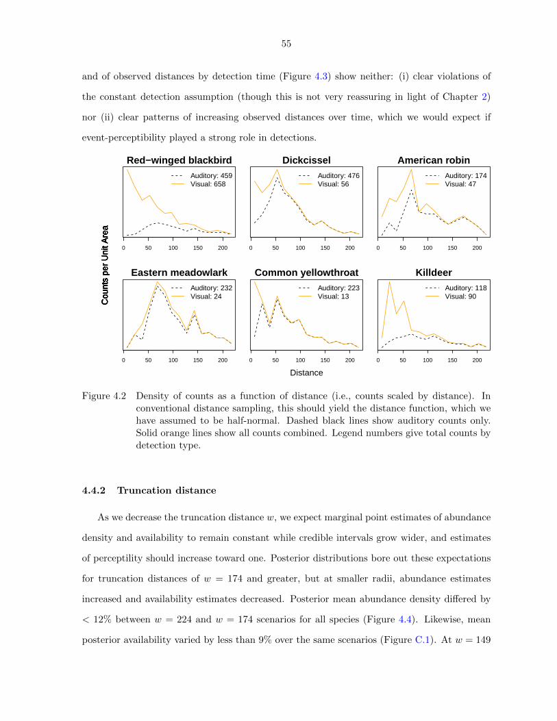
55
and of observed distances by detection time (Figure 4.3) show neither: (i) clear violations of
the constant detection assumption (though this is not very reassuring in light of Chapter 2)
nor (ii) clear patterns of increasing observed distances over time, which we would expect if
event-perceptibility played a strong role in detections.
0 50 100 150 200
Red−winged blackbird
tabl
e(cu
ts[[1
]])/m
idpo
ints
Auditory: 459Visual: 658
Cou
nts
per
Uni
t Are
a
0 50 100 150 200
Dickcissel
tabl
e(cu
ts[[1
]])/m
idpo
ints
Auditory: 476Visual: 56
Cou
nts
per
Uni
t Are
a
0 50 100 150 200
American robin
tabl
e(cu
ts[[1
]])/m
idpo
ints
Auditory: 174Visual: 47
Cou
nts
per
Uni
t Are
a
0 50 100 150 200
Eastern meadowlark
tabl
e(cu
ts[[1
]])/m
idpo
ints
Auditory: 232Visual: 24
Cou
nts
per
Uni
t Are
a
0 50 100 150 200
Common yellowthroat
Distance
tabl
e(cu
ts[[1
]])/m
idpo
ints
Auditory: 223Visual: 13
Cou
nts
per
Uni
t Are
a
0 50 100 150 200
Killdeer
tabl
e(cu
ts[[1
]])/m
idpo
ints
Auditory: 118Visual: 90
Cou
nts
per
Uni
t Are
a
Figure 4.2 Density of counts as a function of distance (i.e., counts scaled by distance). Inconventional distance sampling, this should yield the distance function, which wehave assumed to be half-normal. Dashed black lines show auditory counts only.Solid orange lines show all counts combined. Legend numbers give total counts bydetection type.
4.4.2 Truncation distance
As we decrease the truncation distance w, we expect marginal point estimates of abundance
density and availability to remain constant while credible intervals grow wider, and estimates
of perceptility should increase toward one. Posterior distributions bore out these expectations
for truncation distances of w = 174 and greater, but at smaller radii, abundance estimates
increased and availability estimates decreased. Posterior mean abundance density differed by
< 12% between w = 224 and w = 174 scenarios for all species (Figure 4.4). Likewise, mean
posterior availability varied by less than 9% over the same scenarios (Figure C.1). At w = 149

56
0 1 2 3 4 5
010
020
030
040
050
060
0
Minutes
Cou
nt
AMROCOYEDICKEAMEKILLRWBL
0 100 200 300
0.00
00.
004
0.00
8
Red−winged blackbird
0 100 200 300
0.00
00.
004
0.00
8
Dickcissel
0 100 200 300
0.00
00.
004
0.00
8
American robinMinute
12345
0 100 200 300
0.00
00.
004
0.00
8
Eastern meadowlark
0 100 200 300
0.00
00.
004
0.00
8Common yellowthroat
Distance0 100 200 300
0.00
00.
004
0.00
8
Killdeer
Den
sity
Figure 4.3 Left: Density plots of observed distances conditioned on the time interval of detec-tion. Note: for fifth minute, densities reflect ≤ 20 detections for all but red-wingedblackbirds. Right: Total number of birds detected during each minute of observa-tion.
and w = 99, except for dickcissels, posterior mean abundance density increased on the order of
14-32% and 40-70%, respectively, with credible intervals becoming 30-60% and 40-190% wider.
Posterior availability estimates at w = 149 remained unchanged for most species but dropped
relatively 11-21% for red-winged blackbirds and eastern meadowlarks. At w = 99, for all species
except dickcissels and killdeer, posterior availability declined a total 23-35% with accompanying
increases in posterior perceptibility. Irregularities surfaced for two species at w = 149 —
red-winged blackbirds showed a bimodal posterior such we sometimes encountered with high-
availability / low-perceptibility simulations in Chapter 3, and perceptibility for American robins
strangely declined.
Buckland et al. (2001) recommended choosing w so that g(w) = 0.10. Based on this
standard, most of our models returned truncation points near 170 meters (or 240 meters for
American robins and eastern meadowlarks). The selection of w involves a trade-off between
detection probability and sample size that we have not yet explored enough to make a firm
recommendation. However, considering the consistency of larger-radius estimates and the in-

57
congruity of w = 149 results for two species, for simplicity’s sake we proceed for the rest of this
chapter using the w = 174 for all species. In general, the choice of truncation radius had little
effect on posterior estimates of covariate effects.
●
●
●
●
●
●
●
●
●
●
●
●
●
●
●
●
●
●
●
●
●
●
●
●
●
●
●
●
●
●
Eastern meadowlark Killdeer Red−winged blackbird
American robin Common yellowthroat Dickcissel
10 20 30 40 20 30 40 60 80 100 120 140
10 15 20 25 30 20 30 40 50 60 40 45 50 55 60 65
99
149
174
199
224
99
149
174
199
224
99
149
174
199
224
99
149
174
199
224
99
149
174
199
224
99
149
174
199
224
Estimated Density (per km2)
Trun
catio
n P
oint
Figure 4.4 Caterpillar plots of posterior abundance density marginally across all surveys.Black lines show 95% credible intervals, orange lines show 50% credible intervals,and black dots show posterior medians.
4.4.3 Estimates and inference
The motivating question behind these point-count surveys is whether prairie strip fields host
more birds than rowcropped (control) fields. Figure 4.5 shows expected log-scale abundance
for each treatment-year and compares treatments pairwise averaged across years. Both proxy-
strip and strips sites hosted greater abundance than control sites for dickcissels and red-winged
blackbirds, with proxy-strip sites being more abundant than strips sites for red-winged black-
birds. Strips sites were more abundant than the other treatment sites for common yellowthroat.
Pairwise comparisons within other species had 95% credible intervals that contained zero and
therefore did not attain the usual standard of statistical significance. Still, control treatments
tended to be less abundant than proxy-strips and strips treatments for eastern meadowlarks
and killdeer, respectively.

58
●
●
●
●
●
●
●
●
●
●
●
●
●
●
●
●
●
●
●
●
●
●
●
●
●
●
●
●
●
●
●
●
●
●
●
●
●
●
●
●
●
●
Eastern meadowlark Killdeer Red−winged blackbird
American robin Common yellowthroat Dickcissel
−1 0 1 2 3 −1 0 1 2 3 −1 0 1 2 3
Location StDevStrips 2016Strips 2015Proxy 2016Proxy 2015
Control 2016Control 2015
Location StDevStrips 2016Strips 2015Proxy 2016Proxy 2015
Control 2016Control 2015
Log−Scale Abundance
Trea
tmen
t Effe
cts
●
●
●
●
●
●
●
●
●
●
●
●
●
●
●
●
●
●
Eastern meadowlark Killdeer Red−winged blackbird
American robin Common yellowthroat Dickcissel
−1 0 1 −1 0 1 −1 0 1
Proxy minus StripsControl minus StripsControl minus Proxy
Proxy minus StripsControl minus StripsControl minus Proxy
Log−Scale Abundance
Trea
tmen
t Diff
eren
ces
●
●
●
●
●
●
●
●
●
●
●
●
●
●
●
●
●
●
●
●
●
●
●
●
●
●
●
●
●
●
●
●
●
●
●
●
●
●
●
●
●
●
Eastern meadowlark Killdeer Red−winged blackbird
American robin Common yellowthroat Dickcissel
−1 0 1 2 3 −1 0 1 2 3 −1 0 1 2 3
Location StDevStrips 2016Strips 2015Proxy 2016Proxy 2015
Control 2016Control 2015
Location StDevStrips 2016Strips 2015Proxy 2016Proxy 2015
Control 2016Control 2015
Log−Scale Abundance
Trea
tmen
t Effe
cts
●
●
●
●
●
●
●
●
●
●
●
●
●
●
●
●
●
●
Eastern meadowlark Killdeer Red−winged blackbird
American robin Common yellowthroat Dickcissel
−1 0 1 −1 0 1 −1 0 1
Proxy minus StripsControl minus StripsControl minus Proxy
Proxy minus StripsControl minus StripsControl minus Proxy
Log−Scale Abundance
Trea
tmen
t Diff
eren
ces
Figure 4.5 Posterior estimates of expected log-scale abundance per survey by treatment-year.‘Location StDev’ quantifies location-to-location variability. ‘X minus Y ’ entriesshow pairwise differences between treatments averaged over years. Black linesshow 95% credible intervals, orange lines show 50% credible intervals, and blackdots show posterior medians.
Estimated detection probabilities were low, often below 30% (Figure 4.6). Abundance
estimation at such low detection levels can be unstable to small perturbations in the data
(Olkin et al., 1981). One explanation for the low detection is the use of 5-minute surveys rather
than the 10-minute surveys used in Chapters 2 & 3. Median posterior marginal availability
ranged from 0.46-0.69, but in a 10-minute survey, the same rate of detection cues would result
in availability closer to 0.7-0.9.
Models for all species estimated high event-perceptibility, meaning the observer detected
most or nearly all availability cues. Viewed in terms of data patterns, a high event-perceptibility
reflects that detection distances did not increase appreciably during the survey interval (Figure
4.3). Looking at just the posterior distributions for the log-scale event-perceptibility intercept
term (Figure 4.6), a low-end estimate of 0.5 translates to an average 84% detection probability

59
●
●
●
●
●
●
●
●
●
●
●
●
●
●
●
●
●
●
●
●
●
●
●
●
Density Pr(Detection) Availability Perceptibility
25 50 75 0.2 0.3 0.4 0.3 0.4 0.5 0.6 0.7 0.3 0.4 0.5 0.6 0.7
Red−winged blackbirdKilldeer
Eastern meadowlarkDickcissel
Common yellowthroatAmerican robin
Spe
cies
Figure 4.6 Posterior marginal estimates of abundance density (per km2), detection proba-bility, availability, and perceptibility. By definition, Pr(Detection) = availability× perceptibility. Black lines show 95% credible intervals, orange lines show 50%credible intervals, and black dots show posterior medians.
for any single availability cue at a survey site. Most of the posteriors lie between 1.0-1.5, which
translate to 94-98% detection of availability cues.
Estimates of state-perceptibility were much lower, signifying a classic distance-detection
trend. Posterior distributions for the log-scale state-perceptibility intercept term (Figure 4.7)
closely mirror overall estimates of perceptibility (Figure 4.6) — again illustrating that event-
perceptibility plays a comparatively small role in overall perceptibility. For most species, pos-
terior perceptibility was near 0.4, which was a predictable consequence of choosing the w = 174
truncation point (see Section 4.3.1). These estimates indicate that American robins and eastern
meadowlarks are more readily detected at larger distances than are other species. However,
these two species also evidenced the strongest doughnut-hole effect — i.e., few detections at
near distances (Figure 4.2).
Figure 4.7 shows posterior estimates for availability and perceptibility parameters. Esti-
mates by species across all truncation distances may be found in Figures C.2 – C.7. Killdeer
were the only species to show no signs of subgroup heterogeneity in availability, as seen in
posterior estimation of the mixing parameter and the ‘Easy-Hard Difference’. For all other
species, easy-to-detect birds were nearly always available during the survey (a low easy-to-
detect intercept of -0.5 corresponds to 95% availability during a 5-minute survey). As such,
the mixture of availability rates mainly describes increase of first-interval detections observed
relative to what would be expected from a purely exponential time-to-detection distribution.
Red-winged blackbirds were more often available later in the day, while common yellowthroats

60
were more available early. Most species were more often available early in the year than later,
though dickcissels were available more often later in the season. Examination of random effects
on availability by survey date suggests that the effect of Julian date is actually quadratic for
dickcissels and killdeer, peaking for both 2-3 weeks into June. Likely, this trend accounts for
the high estimates day-to-day variation in availability for these two species. There were no
discernible effects of cloud cover on availability or of wind conditions on event perceptibility.
●
●
●
●
●
●
●
●
●
●
●
●
●
●
●
●
●
●
●
●
●
●
●
●
●
●
●
●
●
●
●
●
●
●
●
●
●
●
●
●
●
●
●
●
●
●
●
●
●
●
●
●
●
●
●
●
●
●
●
●
●
●
●
●
●
●
Event: Intercept Event: Wind State: Intercept
Avail: Time of Day Avail: Julian Date Avail: Cloud Cover Avail: Date StDev
Avail: Hard−to−Detect Avail: Easy−to−Detect Avail: Easy−Hard Diff Avail: Mixing
0 1 2 3 0 1 −0.4 −0.2 0.0 0.2
−0.4 0.0 0.4 −1 0 1 2 −0.4 0.0 0.4 0.0 0.5 1.0 1.5 2.0 2.5
−4 −3 −2 −2 −1 0 1 2 3 0 1 2 3 4 5 0.25 0.50 0.75
RWBLKILL
EAMEDICK
COYEAMRO
RWBLKILL
EAMEDICK
COYEAMRO
RWBLKILL
EAMEDICK
COYEAMRO
RWBLKILL
EAMEDICK
COYEAMRO
RWBLKILL
EAMEDICK
COYEAMRO
RWBLKILL
EAMEDICK
COYEAMRO
RWBLKILL
EAMEDICK
COYEAMRO
RWBLKILL
EAMEDICK
COYEAMRO
RWBLKILL
EAMEDICK
COYEAMRO
RWBLKILL
EAMEDICK
COYEAMRO
RWBLKILL
EAMEDICK
COYEAMRO
Spe
cies
Figure 4.7 Posterior availability and perceptibility estimates. Top row: log-scale availabilityrate intercepts for hard- and easy-to-detect birds, their difference, and the mixingparameter γ giving the proportion of birds that are hard-to-detect. Middle row:covariates on the log-scale availability rate plus random day-to-day availabilityvariability (‘Date StDev’). Bottom row: log-scale intercept terms for event- andstate-perceptibility plus a wind covariate on event-perceptibility. Black lines show95% credible intervals, orange lines show 50% credible intervals, and black dotsshow the posterior mean.
4.5 Discussion
One way to gain insight into a model is to apply it to a not wholly appropriate dataset.
In fitting our two-perceptibility distance-removal model to avian species from the STRIPs

61
experiment, we encountered several violations of assumptions that show the model’s limitations
and point the way to further development. These violations include: pooling of auditory and
visual detections, a doughnut-hole effect, flocks, and maybe non-random location of survey sites.
The inference resulted in apparent contradictions in perceptibility estimates and a heightened
awareness of the role of truncation distance in model results. Based on Chapter 2, we would
like to believe that effect size estimates may be robust to model misspecification, although
abundance estimates will not. However, given the degree of mismatch between our model and
patterns in the STRIPs data, we would be cautious interpreting even effect sizes.
One simple and practical improvement to our model would be to parameterize abundance
in terms of abundance density rather than counts per survey site. This would facilitate com-
parisons of models using different truncation distances. It would also simplify specification of
priors, as the abundance prior would not be influenced by truncation radius.
We modeled auditory and visual cues identically, but Figure 4.2 illustrates that the observed
distance functions for the two modes of detection were clearly different. Visual detections
accounted for most observations at short radius, whereas auditory detections predominated at
distance. To our knowledge, nobody has undertaken to model both detection types for a single
dataset, in part because visual detections rarely account for more than 15% of point-count
survey observations (Alldredge et al., 2007b; Brewster and Simons, 2009). Our results suggest
that this assumption at least merits further investigation. Because our model operates within a
continuous-time parametric survival analysis framework, it is straight-forward conceptually to
accommodate two competing modes of detection, even if it will prove technically more difficult
to implement. A two-mode model would require separate auditory and visual functions for
availability, event-perceptibility, and state-perceptibility. We might first simplify the model by
assuming that auditory state-perceptibility is 100%, thus making the modeled population a
mixture of birds that are and are not visually state-perceptible. For visually state-perceptible
birds, detection rates conditional on radius could then be expressed as the superposition of
homogeneous visual and auditory Poisson processes. Birds that are not state-perceptible would
be detected solely from the auditory Poisson process. Ultimately, this model would result in
two joint distributions of observed distances and times: one for auditory detections and one

62
for visual detections. Because of the need for adequate sample size, the red-winged blackbird
data would be well-suited to this exercise.
A second obstacle to fitting our model was the doughnut-hole effect, which was likely caused
by movement away from the observer (Fewster et al., 2008; Borchers and Cox, 2016). This
pattern can lead to overestimation of perceptibility and underestimation of abundance. It was
clearly evident in STRIPs detections of American robins, eastern meadowlards, and killdeer.
Borchers and Cox (2016) accounted for movement away from observers in a line transect context
by specifying a non-uniform distribution of animals fR(r) in space. Their model had event-
perceptibility but not state-perceptibility, so fR(r) was identifiable with respect to their versions
of the distance function gE(r). However, they noted that models without time-to-detection data
risked confounding between the distribution function fR(r) and the detection function. In the
context of our combined state- and event-perceptibility model, we can see that confounding
arises not from the absence of time-to-detection data per se, but from the inclusion of a state-
perceptibility term. Referring to Eq. (3.10), in our combined model the joint distribution of
detected times and distances is:
fR,T |det(r, t|det) =fR(r)fT |R(t|r)
p(det)I(0 < r < w, 0 < t < C)
=fR(r)gS(r)gE(r)ϕ(t) exp
(−∫ t0 g
E(r)ϕ(u)du)
p(det)I(·)
= fR(r)gS(r)× unrelated terms
so that inference about the doughnut-hole distribution of fR(r) is entirely reliant upon the
chosen forms of fR(r) and gS(r).
For red-winged blackbirds, one-sixth of all detections appeared in clusters of five or more
birds, while half of detections occurred singly. A simple strategy for modeling clusters treats
each flock as an ‘object of interest’ (i.e., single detection) and computes abundance by adjusting
for estimated average flock size; however, if flock size influences detection probability, more
sophisticated methods are needed (Buckland, 2004). The STRIPs data are further complicated
because records of auditory/visual detections for clusters was inconsistent.
Our assumption of uniform avian density relies on the random location of survey sites with

63
respect to the population of interest (Buckland et al., 2001). If sites are not randomly located
with respect to linear features (e.g. roads), we can adjust the density function fR(r) accordingly
(Marques et al., 2010) . While STRIPs survey sites appear to have been placed in a triangular
grid, we do not know design details beyond this. It is possible that the placement of survey
sites relative to prairie strips or habitat beyond field edges influenced model estimates.
Our perceptibility results pose a seeming contradiction: individual availability cues were
detected reliably at large distances (high event-perceptibility), but perceptibility dropped off
considerably within 100 meters (40% state-perceptibility). These results would be sensible for
visual surveys of an eye-catching species on a patchwork landscape, but for largely auditory
counts, they are problemmatic. In terms of data patterns, the estimated state-perceptibility
captures the fact that the number of detections declined with distance. The estimated event-
perceptibility reflects that observed distances did not appreciably change with time during a
survey — phrased differently, the distribution of observed times and distances was not much
different from the independent product of the marginal distributions. We surmise these results
stem from data patterns not mechanistically addressed in the model. The two main suspects
are: (i) competing visual and auditory detections, and (ii) the doughnut effect.
Perceptibility estimates depend upon the chosen truncation distance. Selecting a truncation
point w in distance sampling involves a trade-off. At larger radii, estimated perceptibility
decreases and thereby can lead to large uncertainty in estimated abundance – essentially, large
portions of the analyst-defined survey area provide few observations to inform estimation. At
small radii, truncation gets rid of too many field observations — plus, small radii exacerbate
the impact of movement toward or away from the observer. Conventional distance sampling
recommends choosing w for point-count surveys so that perceptibility is roughly 0.40. However,
our model featues a second type of perceptibility plus an availability term that are not part of
conventional distance sampling. Further, we noted in Chapter 3 that abundance estimates for
low-perceptibility species can be biased low when availability is also low. We believe traditional
standards for selecting a truncation distance may not apply to our model. We intend to augment
Chapter 3 with an additional simulation study quantifying the bias and uncertainty that results
from selecting a truncation radius.

64
The bulk of issues described above are well-known challenges in distance modeling with
an established literature exploring them and strategizing remedies. While those strategies are
transferrable to our model, their implementations unfortunately are not. For every change
to assumptions about availability, perceptibility, or population distribution in our model, we
must rederive the calculations for the joint distribution of observed times and distances. The
constant-rate, half-normal-distance, uniform-density model we have exhibited is the easy sce-
nario. For most other forms, none of the integrals are analytic, so each modification requires
new numerical approximations for detection probabilities. If this model is to be broadly fea-
sible, we will need to develop a more flexible, perhaps approximate, method for incorporating
changes.

65
CHAPTER 5. CONCLUSION
We have proposed two classes of models that leverage detection time and distance patterns
in order to estimate abundance from single-species removal-sampled point-count data. These
models implement continuous-time parametric survival analysis of detections within a hierar-
chical N-mixture framework, thereby modeling mixed effects for abundance, availability, and
perception. In terms of the generic posterior distribution from Equation (3.1):
p(θ|n(obs), r, t) ∝ p(n(obs)|θ, p(det)
)(∏i=1
f (ri, ti|θ, p(det))
)p(θ) (5.1)
our models utilize the observed distributions of time and distance — f (ri, ti|θ, p(det)) — in
order to more accurately and flexibly estimate detection and its related parameters. Each
model extends the range of hypotheses that can be addressed with these kinds of data.
In Chapter 2, we formulated a removal-only model that allows detection rates to change
systematically during a survey period. We demonstrated that time-to-detection distributions
(TTDDs) based on two-parameter families (e.g. gamma) provide a flexible alternative to the
standard assumption of constant detection rates. The constant rate assumption, on the other
hand, can be rather too informative, leading to biased, overly precise abundance estimates.
We recommend that non-constant TTDDs be used in analyses where abundance estimation
is a primary objective. However, if abundance and detection effect estimates are the primary
objective, our results suggest these may be robust to the choice of TTDD. Relative abundance
estimates obtained from constant-detection models may still be useful if treated as a kind of
detection-weighted index for abundance (Johnson, 2008). Further research is required on this
question.
In Chapters 3, we reconciled two distinct approaches to distance-removal modeling, one
emphasizing detectable animals and the other emphasizing detectable cues. In the process,

66
we defined two types of perceptibility and clarified their relationship to availability. Our sim-
ulations showed that single-perceptibility state and event models return differing inference,
especially under conditions of low perceptibility and high availability. We combined both per-
ceptibility types into a single model which frames detection as a four-stage process requiring:
presence, state perceptibility, availability, and perception of at least one availability event. This
combined state-event model yielded accurate abundance estimates across all scenarios. Based
on these results, we recommend implementing a dual-perceptibility approach for all distance-
removal models.
In Chapter 4, we evaluated the four-stage distance-removal model by applying it to point-
count surveys of six species from the STRIPs project at Iowa State University. Several data
features violated model assumptions, pointing to model limitations and directions for its im-
provement. Problematic data features included the pooling of auditory and visual detections,
movement of animals away from the observer, flocks, and linear habitat structures. Future
improvements for the model should prioritize: (i) guidelines for identifying of an appropriate
distance truncation radius, and (ii) flexibility in the calculation of the joint distribution of ob-
served times and distances so that users can easily change forms of the abundance, availability,
and perceptibility models.
5.1 Data considerations
Models of detection rely upon extrapolating a pattern of times and distances for observed
individuals — f (ri, ti|θ, p(det)) from Equation (5.1) — to realistically describe the pattern
for unobserved individuals. If a chosen TTDD and/or perceptibility model fails to adequately
describe either observed and/or unobserved detection patterns, then abundance estimates will
be wrong. From our vantage as modelers, some modifications to data collection could improve
model performance. The basic strategies are: (i) more exact data, (ii) longer surveys (iii) more
complete data, and (iv) less distorted data. We discuss these with a focus on avian surveys.
With the advent of laser range finders, observers already collect exact distances (within
practicality). If observers can also collect exact detection times, then model precision should
improve, though due to observer saturation this may be easier said than done. Early in our

67
explorations, we fit constant-rate removal-only models to 10-minutes surveys censored into three
or nine intervals. Detection parameter credible intervals were roughly 20% narrower when using
the nine-interval data. We likewise expect that analyses based on exact data will yield more
precise results than those based on interval-censored data. A simulation study could quantify
the benefit of using exact times relative to interval-censoring under various scenarios. Using
exact distances and times can also speed MCMC sampling. Calculating the joint distribution
for each observation f (ri, ti|θ, p(det)) is a simple functional evaluation for exact data, but
for interval-censored data, it involves integration across the censored units. When analytic
solutions are available (e.g. the simple scenario used in Chapters 3 & 4), we can bypass the
integration step, but when they are not available, numeric integration will be required for every
observation within each MCMC iteration.
Longer surveys could provide better estimation of TTDD shape and detection probability.
However, birds are mobile and a 10-minute survey already stretches credulity in terms of
population closure (Lee and Marsden, 2008; Reidy et al., 2011; Hutto, 2016). We think that
well-designed longer duration studies could supplement point-count surveys, with availability
information being transmitted through model priors. Diefenbach et al. (2007) conducted one-
hour observations of sparrows that had been tagged and fitted with radiotransmitters. Such
a long-term observation potentially provides a good characterization of TTDDs over time.
Unfortunately, the methodology is labor-intense and only monitors a few birds at any time.
Alldredge et al. (2007a) proposed the collection of complete detection history data. Censor-
ing observations in time, they recorded every interval during which each bird sang rather than
just the first interval. Although our models are not constructed for complete detection data,
we endorse this approach because it retains all observations and potentially helps to charac-
terize behavioral subgroups (hard- and easy-to-detect). Drawbacks are that this may become
overwhelming for an observer in a multi-species study, and repeat observations of an individual
are not independent.
A major concern of ours has been the distortion of theoretical distributions used in modeling,
especially due to observer effects. Our use of two-parameter TTDDs can approximate observer
effects in removal-only models, but if we assume that observer effects diminish with distance,

68
this has the potential to be a more complex problem in distance-removal models. Therefore,
design-based solutions are desireable. Settling down periods at the outset of a survey may
address the non-constant detection dimension of this problem, but they come at a heavy cost
in terms of total count and distortions to the spatial distribution of animals (Lee and Marsden,
2008).
We are hopeful about advances in microphone surveys. Microphone arrays have the poten-
tial to address every one of the above issues, yielding exact-time, unlimited-duration, complete-
history, observer-free detections. Campbell and Francis (2012) used microphone arrays to test
for observer effects. They monitored sites before and during observer-conducted avian point-
count surveys and found no change in microphone-recorded detection rates or distances. To be
sure, there are technological obstacles to overcome, including identification and classification
of individual calls, triangulation of distances under varying conditions, and data management
(Blumstein et al., 2011).
5.2 Modeling considerations
Our top priority for model development is a simulation study for choosing the truncation
point w for the distance-removal model. Buckland et al. (2001) suggest selecting w in a con-
ventional distance sampling point-count analysis so that perceptibility is roughly 0.40, but our
model is more complex due to the additions of an availability model and an event-perceptibility
model. Further, our simulation results from Chapter 3 for models fit to low-perceptibility (0.40)
datasets suggest that abundance estimates may be biased when availability is low. A simulation
study should help characterize the trade-off between uncertainty at large radii versus sample
size at small radii.
We have utilized simulation studies to quantify bias and coverage over a large number of
model fits, but we have not delved into model diagnostics for evaluating single model fits, nor
selection tools for comparing related models fit to the same dataset. Early efforts in these
directions have not been promising with regard to time-to-detection data. Posterior predictive
checks based on the marginal distribution of detection times only showed clear misspecification
for the most egregious of model misfits in Chapter 2. Likewise, comparison of DIC values led

69
to correct model selection for only the same set of egregious scenarios, and it also sometimes
produced erroneous selection. In Chapter 3, the ∆elpd statistic (based on leave-one-out in-
formation criterion and related to WAIC) only pointed to the correct state or event model in
scenarios of where they most sharply contrasted, and it was not consistently informative in
scenarios featuring abundance bias from 15% to as high as 50%. For both model diagnostics
and model comparison, the main barricade to progress with time-to-detection data is extrap-
olation. A wide variety of models can provide reasonable fits for detected individuals while
differing substantially in predictions for unobserved individuals. There is no way to choose
between such models without either collecting extra data or imposing assumptions. We are
not concerned about goodness-of-fit for the distance component of the data. The established
method is to bin distance observations and calculate χ2 statistics (Buckland et al., 2001). Es-
pecially in state models, which treat distance events as independent from time events, we see
no reason to doubt the existing method.
One obvious continuation of our research is to merge the models from Chapters 2 & 3
and create a non-constant detection distance-removal model. We have already established the
theoretical architecture for this in Chapter 3; it ‘just’ remains to implement the calculations. Of
the three TTDDs we considered, we recommend beginning with a Weibull for the distribution
of detection times given distance fT |R(t|r). In simulations, the Weibull generally seemed more
accurate than the lognormal. Meanwhile, we want to avoid the gamma distribution because it
has a non-analytic cdf, meaning that calculations of ps(det) =∫ w0
∫ C0 fT |R(t|r)fR(r)dtdr from
Section 3.3.4 would require a double numeric integration.
As with modeling non-constant detection, we also would like the flexibility to model per-
ceptibility functions gE(r) and gS(r) as other than half-normal. The flexibility of perceptibility
functions in conventional distance sampling is one of the chief attractions of the approach.
In particular, the distance function can be modeled using a key function plus series adjust-
ment (Buckland et al., 2001; Miller and Thomas, 2015), which is flexible enough to conform to
many empirical distributions. Assuming constant-rate detection, calculations for p(det) in our

70
combined model (Equation (B.26))
p(det) =2
w2
w∫0
rgS(r)[1− e−gE(r)ϕC
]dr (5.2)
would become as complicated as the proposed perceptibility functions, but would only require
a single integration:
In general, the integrations required to calculate detection probabilities limit the flexibility
of our distance-removal model. If we wish to make model implementation more broadly feasible,
we must explore improvements. At present, our hierarchical model consists of four sub-models
plus a site-level animal distribution function: abundance, availability, state perceptibility, and
event perceptibility, plus fR(r). Each has an assumed form — right now, those are Poisson,
exponential, half-normal, half-normal, and uniform, respectively. Changes to any of these (ex-
cept abundance) necessitate derivation of a new integral to obtain p(det), and as things stand,
that requires a new numerical integration/approximation. This can also add a computational
burden if data are interval-censored in distance or time, because the MCMC sampling may
additionally involve numerical integrations for each observation during each MCMC iteration.
We think step-function approximations of distance-related functions would lead to simpler
computations and greater flexibility with regard to the selection of perceptibility functions.
The basic idea is to replace the joint distribution of observed times and distances
f (r, t|θ, p(det)) =f (r, t|θ)
p(det|θ)
from Equation (5.1) with an approximation
f (r, t|θ, p(det)) ≈ f (r, t|θ)
p(det|θ)
where p(det|θ) is based on the step-function approximations. At present, during each sampling
iteration our Stan model calculates p(det|θ) for each survey using a series approximation to
Equation (3.16) implemented through integration by parts (see Equation (B.31)). If we want to
change perceptibility functions with the current code, we would need to re-derive both Equa-
tion (3.16) and Equation (B.31). Step-function approximations would make it easier to code
changes to the perceptibility functions. Step-function approximations replace the integration

71
over distance with a summation over distance increments:
p(det|θ) =∑r∈Rj
fR(r)
C∫0
fT |R(t|r) dt
(5.3)
where Rj are increments of the approximating step functions over which gS(r), gE(r), and
fR(r) take constant values. The integral in Equation (5.3) is just a scaled cdf of the distance-
dependent TTDD, recalling from Equation (3.10):
fT |R(t|r) = gSs (r)gEs (r)ϕs(t) exp
(−∫ t
0gEs (r)ϕs(u)
)(5.4)
The key point is: if we want to change the perceptibility functions gS(r) and/or gE(r), then we
only need to recode the functions for gS(r) and gE(r); we do not need to rederive an integral
with respect to distance or its series approximation.

72
APPENDIX A. SUPPORTING TABLES AND FIGURES FOR
CHAPTER 2
Tables
Family Mixture Peaked γ ϕ α
Exponential Non-mixture -1.827
Mixture 0.65 -2.138
Gamma Non-mixture Nonpeaked -3.279 0.257
Peaked -0.746 3.371
Mixture Nonpeaked 0.65 -2.773 0.577
Peaked 0.65 -1.210 2.491
Lognormal Non-mixture Nonpeaked -0.341 2.330
Peaked -1.872 0.512
Mixture Nonpeaked 0.65 -1.462 1.674
Peaked 0.65 -1.992 0.618
Weibull Non-mixture Nonpeaked -1.165 0.418
Peaked -2.042 1.829
Mixture Nonpeaked 0.65 -2.063 0.687
Peaked 0.65 -2.201 1.621
Table A.1 Table of parameter values used to generate data for: (i) the mixture vs. non-mix-ture simulation, and (ii) the constant vs. non-constant rate simulation. Here γis a mixing parameter for the proportion of ‘hard to detect’ individuals, ϕ is thedetection rate parameter, and α is the shape parameter.

73
Family
Mixture
Peak
βA 1
βA 2
βA 3
βA 4
βD 1
βD 2
βD 3
βD 4
βD 5
Exponen
tial
Non-m
ixture
0.122
0.002
0.094
-1.039
-0.01
-0.056
0.118
0.249
0.164
Mixture
0.124
0.012
0.064
-1.07
-0.068
-0.146
0.03
0.312
0.27
Gamma
Non-m
ixture
Nonpeaked
0.129
-0.001
0.098
-1.039
0.048
-0.104
-0.12
0.141
0.129
Peaked
0.129
-0.001
0.098
-1.039
0.048
-0.104
-0.12
0.141
0.129
Mixture
Nonpeaked
0.128
-0.005
0.079
-1.051
-0.048
-0.126
-0.042
0.21
0.2
Peaked
0.128
-0.005
0.079
-1.051
-0.048
-0.126
-0.042
0.21
0.2
Lognorm
al
Non-m
ixture
Nonpeaked
0.126
0.031
0.096
-1.047
0.163
-0.099
-0.071
0.31
0.079
Peaked
0.126
0.031
0.096
-1.047
0.163
-0.099
-0.071
0.31
0.079
Mixture
Nonpeaked
0.126
0.017
0.07
-1.068
0.006
-0.14
-0.038
0.341
0.191
Peaked
0.126
0.017
0.07
-1.068
0.006
-0.14
-0.038
0.341
0.191
Weibull
Non-m
ixture
Nonpeaked
0.129
0.011
0.102
-1.04
0.101
-0.104
-0.127
0.204
0.086
Peaked
0.129
0.011
0.102
-1.04
0.101
-0.104
-0.127
0.204
0.086
Mixture
Nonpeaked
0.129
-0.002
0.081
-1.049
-0.028
-0.122
-0.069
0.204
0.183
Peaked
0.129
-0.002
0.081
-1.049
-0.028
-0.122
-0.069
0.204
0.183
Family
Mixture
Peak
Intercep
tAIntercep
tDσA1
σA2
σD
γα
Exponential
Non-m
ixture
0.975
-1.146
0.139
0.094
0.242
Mixture
1.097
-1.97
0.13
0.091
0.259
0.647
Gamma
Non-m
ixture
Nonpeaked
1.383
-3.941
0.121
0.072
0.39
0.316
Peaked
1.134
-0.746
0.121
0.072
0.39
3.371
Mixture
Nonpeaked
1.215
-2.7
0.121
0.079
0.332
0.79
0.597
Peaked
1.134
-1.21
0.121
0.079
0.332
0.65
2.491
Lognorm
al
Non-m
ixture
Nonpeaked
1.613
-2.444
0.151
0.077
0.353
3.287
Peaked
1.134
-1.872
0.151
0.077
0.353
0.512
Mixture
Nonpeaked
1.282
-2.051
0.14
0.079
0.312
0.706
1.467
Peaked
1.134
-1.992
0.14
0.079
0.312
0.65
0.618
Weibull
Non-m
ixture
Nonpeaked
1.57
-3.137
0.131
0.074
0.383
0.387
Peaked
1.134
-2.042
0.131
0.074
0.383
1.829
Mixture
Nonpeaked
1.294
-2.354
0.122
0.078
0.344
0.814
0.653
Peaked
1.134
-2.201
0.122
0.078
0.344
0.65
1.621
Tab
leA
.2T
ab
leof
par
amet
erva
lues
use
dto
gen
erat
ed
ata
for
sim
ula
tion
sw
ith
cova
riat
es(S
ecti
on2.
4.3)
.H
ere,γ
isa
mix
ing
par
amet
erfo
rth
ep
rop
orti
onof
‘hard
tod
etec
t’in
div
idu
als,β
’sar
efi
xed
effec
ts,σ
’sar
era
nd
omeff
ect
stan
dar
dd
evia
tion
s,α
isa
shap
ep
aram
eter
,an
dsu
per
scri
pts
ofA
andD
ind
icat
eab
un
dan
cean
dd
etec
tion
par
amet
ers,
resp
ecti
vely
.

74
Non-mixture model Mixture modelMed p Q(p) 50% 90% Med p Q(p) 50% 90%
TTDD
usedto
simulate
data
Non-m
ixture
Nonpk. Gamma 0.67 0.84 0.11 0.94 0.76 0.92 0.00 0.70
Lognormal 0.54 0.60 0.81 1.00 0.68 0.88 0.05 0.79Weibull 0.55 0.61 0.79 0.99 0.69 0.84 0.16 0.87Exponential 0.49 0.45 0.51 0.93 0.45 0.30 0.47 0.86
Peaked Gamma 0.48 0.46 0.57 0.90 0.57 0.72 0.42 0.85
Lognormal 0.49 0.45 0.53 0.93 0.54 0.69 0.37 0.89Weibull 0.48 0.48 0.40 0.91 0.59 0.74 0.37 0.80
Mixture Nonpk. Gamma 0.62 0.76 0.42 0.99 0.71 0.86 0.10 0.89
Lognormal 0.50 0.47 0.95 1.00 0.64 0.84 0.09 0.97Weibull 0.50 0.47 0.92 1.00 0.64 0.77 0.39 0.98Exponential 0.88 1.00 0.00 0.00 0.50 0.49 0.54 0.95
Peaked Gamma 0.24 0.01 0.00 0.00 0.52 0.53 0.76 0.99
Lognormal 0.18 0.00 0.00 0.00 0.49 0.47 0.66 0.97Weibull 0.18 0.00 0.00 0.00 0.52 0.52 0.80 1.00
Table A.3 Summary of mixture vs. non-mixture model fits when the detection probability isp(det) = 0.50. In all cases, the inference model family matches the dataset family.Med p: average across simulations of the posterior median of p(det). Q(p): averageproportion of the posterior distribution of p(det) that is larger than the true value.50% and 90% coverage is expressed as the proportion of 100 simulations for whichthe true value of p(det) lies within the appropriate credible interval.
Non-mixture model Mixture modelMed p Q(p) 50% 90% Med p Q(p) 50% 90%
TTDD
usedto
simulate
data
Non-m
ixture
Nonpk. Gamma 0.69 0.59 0.78 0.98 0.78 0.79 0.35 0.90
Lognormal 0.59 0.31 0.45 0.91 0.73 0.69 0.63 0.90Weibull 0.60 0.38 0.59 0.99 0.73 0.68 0.59 0.94Exponential 0.64 0.47 0.50 0.85 0.61 0.29 0.33 0.82
Peaked Gamma 0.64 0.44 0.46 0.89 0.68 0.66 0.51 0.85
Lognormal 0.64 0.47 0.36 0.87 0.67 0.63 0.44 0.79Weibull 0.61 0.40 0.46 0.88 0.69 0.67 0.46 0.88
Mixture Nonpk. Gamma 0.60 0.36 0.78 1.00 0.71 0.63 0.81 0.99
Lognormal 0.52 0.13 0.12 0.74 0.67 0.54 0.93 1.00Weibull 0.51 0.17 0.23 0.82 0.66 0.52 0.92 1.00Exponential 0.93 1.00 0.00 0.00 0.63 0.46 0.45 0.87
Peaked Gamma 0.26 0.00 0.00 0.00 0.58 0.34 0.51 0.95
Lognormal 0.20 0.00 0.00 0.00 0.61 0.41 0.58 0.92Weibull 0.19 0.00 0.00 0.00 0.56 0.34 0.44 0.95
Table A.4 Summary of mixture vs. non-mixture model fits when the detection probability isp(det) = 0.65. In all cases, the inference model family matches the dataset family.Med p: average across simulations of the posterior median of p(det). Q(p): averageproportion of the posterior distribution of p(det) that is larger than the true value.50% and 90% coverage is expressed as the proportion of 100 simulations for whichthe true value of p(det) lies within the appropriate credible interval.

75
Non-mixture model Mixture modelMed p Q(p) 50% 90% Med p Q(p) 50% 90%
TTDD
usedto
simulate
data
Non-m
ixture
Nonpk. Gamma 0.75 0.39 0.45 0.92 0.83 0.62 0.55 0.91
Lognormal 0.71 0.29 0.29 0.82 0.82 0.61 0.63 0.91Weibull 0.72 0.34 0.41 0.86 0.82 0.60 0.59 0.93Exponential 0.80 0.49 0.54 0.88 0.78 0.32 0.48 0.86
Peaked Gamma 0.79 0.44 0.45 0.87 0.81 0.59 0.45 0.90
Lognormal 0.80 0.48 0.52 0.95 0.81 0.60 0.53 0.92Weibull 0.78 0.37 0.38 0.84 0.81 0.57 0.49 0.92
Mixture Nonpk. Gamma 0.64 0.11 0.11 0.59 0.75 0.38 0.64 1.00
Lognormal 0.58 0.06 0.04 0.27 0.74 0.33 0.51 0.98Weibull 0.54 0.04 0.01 0.23 0.70 0.27 0.46 1.00Exponential 0.96 1.00 0.00 0.00 0.78 0.45 0.42 0.86
Peaked Gamma 0.28 0.00 0.00 0.00 0.72 0.30 0.40 0.80
Lognormal 0.22 0.00 0.00 0.00 0.78 0.45 0.46 0.87Weibull 0.22 0.00 0.00 0.00 0.69 0.29 0.33 0.88
Table A.5 Summary of mixture vs. non-mixture model fits when the detection probability isp(det) = 0.80. In all cases, the inference model family matches the dataset family.Med p: average across simulations of the posterior median of p(det). Q(p): averageproportion of the posterior distribution of p(det) that is larger than the true value.50% and 90% coverage is expressed as the proportion of 100 simulations for whichthe true value of p(det) lies within the appropriate credible interval.
Non-mixture model Mixture modelMed p Q(p) 50% 90% Med p Q(p) 50% 90%
TTDD
usedto
simulate
data
Non-m
ixture
Nonpk. Gamma 0.95 0.44 0.59 0.95 0.96 0.62 0.61 0.96
Lognormal 0.94 0.42 0.47 0.87 0.96 0.65 0.44 0.90Weibull 0.94 0.46 0.43 0.90 0.96 0.67 0.52 0.84Exponential 0.95 0.54 0.48 0.90 0.94 0.37 0.42 0.89
Peaked Gamma 0.95 0.43 0.44 0.89 0.95 0.50 0.40 0.88
Lognormal 0.95 0.50 0.44 0.88 0.95 0.54 0.44 0.88Weibull 0.95 0.53 0.49 0.91 0.96 0.65 0.42 0.85
Mixture Nonpk. Gamma 0.85 0.04 0.03 0.22 0.91 0.25 0.31 0.77
Lognormal 0.85 0.03 0.03 0.16 0.92 0.28 0.38 0.86Weibull 0.71 0.01 0.01 0.02 0.87 0.22 0.28 0.68Exponential 0.99 1.00 0.00 0.00 0.94 0.41 0.51 0.85
Peaked Gamma 0.37 0.00 0.00 0.00 0.94 0.39 0.41 0.83
Lognormal 0.27 0.00 0.00 0.00 0.94 0.40 0.43 0.83Weibull 0.28 0.00 0.00 0.00 0.93 0.36 0.47 0.80
Table A.6 Summary of mixture vs. non-mixture model fits when the detection probability isp(det) = 0.95. In all cases, the inference model family matches the dataset family.Med p: average across simulations of the posterior median of p(det). Q(p): averageproportion of the posterior distribution of p(det) that is larger than the true value.50% and 90% coverage is expressed as the proportion of 100 simulations for whichthe true value of p(det) lies within the appropriate credible interval.

76
Exponential mixture model Gamma mixture model
Med p Q(p) 50% 90% Med p Q(p) 50% 90%
Data
Mixture
Nonpk. Gamma 0.84 0.99 0.00 0.05 0.71 0.86 0.10 0.89
Lognormal 0.89 1.00 0.00 0.00 0.78 0.93 0.01 0.56Weibull 0.86 1.00 0.00 0.02 0.73 0.89 0.03 0.82Exponential 0.50 0.49 0.54 0.95 0.54 0.57 0.84 1.00
Peaked Gamma 0.31 0.06 0.05 0.32 0.52 0.53 0.76 0.99
Lognormal 0.26 0.02 0.00 0.09 0.59 0.68 0.52 0.91Weibull 0.30 0.05 0.05 0.28 0.49 0.46 0.75 1.00
Lognormal mixture model Weibull mixture model
Med p Q(p) 50% 90% Med p Q(p) 50% 90%
Data
Mixture
Nonpk. Gamma 0.63 0.80 0.23 0.99 0.63 0.74 0.54 0.98
Lognormal 0.64 0.84 0.09 0.97 0.68 0.83 0.21 0.95Weibull 0.63 0.81 0.18 0.99 0.64 0.77 0.39 0.98Exponential 0.49 0.45 0.77 1.00 0.54 0.56 0.87 0.99
Peaked Gamma 0.45 0.36 0.60 1.00 0.55 0.58 0.77 0.98
Lognormal 0.49 0.47 0.66 0.97 0.64 0.75 0.43 0.87Weibull 0.43 0.30 0.51 0.97 0.52 0.52 0.80 1.00
Table A.7 Summary of models fits across family of TTDD when true detection probabilityis p(det) = 0.50. All data and inference models have mixture components. Medp: average across simulations of the posterior median of p(det). Q(p): averageproportion of the posterior distribution of p(det) that is larger than the true value.50% and 90% coverage is expressed as the proportion of simulations for which thetrue value of p(det) lies within the appropriate credible interval.
Exponential mixture model Gamma mixture model
Med p Q(p) 50% 90% Med p Q(p) 50% 90%
Data
Mixture
Nonpk. Gamma 0.83 0.96 0.04 0.21 0.71 0.63 0.81 0.99
Lognormal 0.91 1.00 0.00 0.00 0.82 0.86 0.19 0.70Weibull 0.87 0.98 0.01 0.09 0.75 0.72 0.54 0.97Exponential 0.63 0.46 0.45 0.87 0.60 0.38 0.70 1.00
Peaked Gamma 0.33 0.01 0.02 0.05 0.58 0.34 0.51 0.95
Lognormal 0.30 0.00 0.00 0.00 0.71 0.68 0.48 0.88Weibull 0.32 0.00 0.00 0.00 0.53 0.25 0.31 0.89
Lognormal mixture model Weibull mixture model
Med p Q(p) 50% 90% Med p Q(p) 50% 90%
Data
Mixture
Nonpk. Gamma 0.63 0.43 0.87 1.00 0.63 0.45 0.94 1.00
Lognormal 0.67 0.54 0.93 1.00 0.73 0.66 0.68 0.98Weibull 0.64 0.46 0.97 1.00 0.66 0.52 0.92 1.00Exponential 0.55 0.24 0.39 0.95 0.58 0.36 0.69 1.00
Peaked Gamma 0.50 0.16 0.21 0.65 0.62 0.44 0.59 0.98
Lognormal 0.61 0.41 0.58 0.92 0.77 0.79 0.34 0.78Weibull 0.47 0.11 0.13 0.48 0.56 0.34 0.44 0.95
Table A.8 Summary of models fits across family of TTDD when true detection probabilityis p(det) = 0.65. All data and inference models have mixture components. Medp: average across simulations of the posterior median of p(det). Q(p): averageproportion of the posterior distribution of p(det) that is larger than the true value.50% and 90% coverage is expressed as the proportion of simulations for which thetrue value of p(det) lies within the appropriate credible interval.

77
Exponential mixture model Gamma mixture model
Med p Q(p) 50% 90% Med p Q(p) 50% 90%
Data
Mixture
Nonpk. Gamma 0.86 0.83 0.25 0.59 0.75 0.38 0.64 1.00
Lognormal 0.93 1.00 0.00 0.01 0.88 0.80 0.33 0.72Weibull 0.89 0.93 0.11 0.36 0.79 0.49 0.66 0.99Exponential 0.78 0.45 0.42 0.86 0.70 0.25 0.32 0.91
Peaked Gamma 0.37 0.00 0.00 0.00 0.72 0.30 0.40 0.80
Lognormal 0.34 0.00 0.00 0.00 0.85 0.77 0.24 0.65Weibull 0.38 0.00 0.00 0.00 0.65 0.16 0.22 0.54
Lognormal mixture model Weibull mixture model
Med p Q(p) 50% 90% Med p Q(p) 50% 90%
Data
Mixture
Nonpk. Gamma 0.65 0.16 0.16 0.85 0.67 0.23 0.34 0.99
Lognormal 0.74 0.33 0.51 0.98 0.81 0.55 0.59 0.97Weibull 0.66 0.17 0.22 0.87 0.70 0.27 0.46 1.00Exponential 0.61 0.11 0.12 0.52 0.64 0.21 0.24 0.85
Peaked Gamma 0.64 0.09 0.10 0.41 0.77 0.49 0.46 0.93
Lognormal 0.78 0.45 0.46 0.87 0.90 0.90 0.13 0.40Weibull 0.57 0.04 0.02 0.19 0.69 0.29 0.33 0.88
Table A.9 Summary of models fits across family of TTDD when true detection probabilityis p(det) = 0.80. All data and inference models have mixture components. Medp: average across simulations of the posterior median of p(det). Q(p): averageproportion of the posterior distribution of p(det) that is larger than the true value.50% and 90% coverage is expressed as the proportion of simulations for which thetrue value of p(det) lies within the appropriate credible interval.
Exponential mixture model Gamma mixture model
Med p Q(p) 50% 90% Med p Q(p) 50% 90%
Data
Mixture
Nonpk. Gamma 0.94 0.30 0.38 0.83 0.91 0.25 0.31 0.77
Lognormal 0.97 0.91 0.07 0.44 0.96 0.72 0.46 0.82Weibull 0.94 0.29 0.37 0.76 0.91 0.25 0.32 0.76Exponential 0.94 0.41 0.51 0.85 0.92 0.26 0.33 0.82
Peaked Gamma 0.55 0.00 0.00 0.00 0.94 0.39 0.41 0.83
Lognormal 0.47 0.00 0.00 0.00 0.97 0.80 0.27 0.65Weibull 0.57 0.00 0.00 0.00 0.89 0.08 0.09 0.43
Lognormal mixture model Weibull mixture model
Med p Q(p) 50% 90% Med p Q(p) 50% 90%
Data
Mixture
Nonpk. Gamma 0.81 0.11 0.10 0.35 0.87 0.23 0.22 0.68
Lognormal 0.92 0.28 0.38 0.86 0.95 0.55 0.57 0.92Weibull 0.82 0.10 0.15 0.34 0.87 0.22 0.28 0.68Exponential 0.82 0.09 0.09 0.38 0.88 0.20 0.25 0.65
Peaked Gamma 0.91 0.09 0.10 0.42 0.97 0.79 0.26 0.63
Lognormal 0.94 0.40 0.43 0.83 0.98 0.98 0.01 0.12Weibull 0.84 0.01 0.00 0.03 0.93 0.36 0.47 0.80
Table A.10 Summary of models fits across family of TTDD when true detection probabilityis p(det) = 0.95. All data and inference models have mixture components. Medp: average across simulations of the posterior median of p(det). Q(p): averageproportion of the posterior distribution of p(det) that is larger than the true value.50% and 90% coverage is expressed as the proportion of simulations for which thetrue value of p(det) lies within the appropriate credible interval.

78
Figures
Gamm nonpeak Logn nonpeak Weib nonpeak Exponential Gamm peak Logn peak Weib peak
●
●
●
●
●
●
●
●
●
●
●
●
●
●
●
●
●
●
●
●
●
●
●
●
●
●
●
●
Weibull
Lognormal
Gamma
Exponential
0.5
0.7
0.9
0.5
0.7
0.9
0.5
0.7
0.9
0.5
0.7
0.9
0.5
0.7
0.7
0.9
0.3
0.5
0.7
Detection Probability
Infe
renc
e M
odel
Figure A.1 Caterpillar plots of posterior estimates of p(det) from Section 2.4.3. Black linesshow 95% credible intervals, orange lines show 50% credible intervals, and blackdots show posterior medians. ‘X’ marks the expected marginal probability ofdetection based on true parameter values. Data and models include fixed andrandom effects for both abundance and detection processes. All data and inferencemodels include mixture components. Each plot presents one simulated dataset.

79
●
●
●
●
●
●
●
●
●
●
●
●
●
●
●
●
●
●
● ●
●
●
●
●
●
●
●
●
●
β1A β2
A β3A β4
A
β1D β2
D β3D β4
D
β5D γ InterceptA InterceptD
σA12 σA2
2 σD2
Exponential
Exponential Mix
Exponential
Exponential Mix
Exponential
Exponential Mix
Exponential
Exponential Mix
0.00 0.05 0.10 0.15 0.20 −0.2 −0.1 0.0 0.0 0.2 0.4 −1.50 −1.25 −1.00 −0.75
−0.2 −0.1 0.0 0.1 −0.20 −0.15 −0.10 −0.05 0.00 0.10 0.15 0.20 0.25 0.30 0.350.1 0.2 0.3 0.4 0.5 0.6
0.0 0.1 0.2 0.3 0.4 0.90 0.95 1.00 0.6 0.8 1.0 −1.4 −1.2 −1.0
0.0 0.1 0.2 0.3 0.1 0.2 0.3 0.1 0.2 0.3 0.4 0.5
Parameter Estimate
Mod
el
Data: Exponential
Figure A.2 Caterpillar plots of posterior parameter estimates from all models fit to the simu-lated non-mixture exponential dataset (from simulations involving covariates andrandom effects). Black and orange lines depict central 95% and 50% credibleintervals, respectively. The black dot is the posterior meadian. The blue ’X’ isthe true parameter value and is positioned on the correctly specified model. β’sare fixed effect parameters, σ’s are random effect standard deviations, and γ is amixing parameter. Parameters designated with an ’A’ are abundance parameters;those designated with a ’D’ are detection parameters.

80
●
●
●
●
●
●
●
●
●
●
●
●
●
●
●
●
●
●
●
●
●
●
●
●
●
●
●
●
●
●
●
●
●
●
●
●
●
●
●
●
●
●
●
●
●
●
●
●
●
●
●
●
●
●
●
●
●
●
●
●
●
●
●
●
●
●
●
●
●
●
●
●
●
●
●
●
●
β1A β2
A β3A β4
A
β1D β2
D β3D β4
D
β5D γ InterceptA InterceptD
Shape σA12 σA2
2 σD2
ExponentialExponential Mix
Gamma MixLognormal Mix
Weibull Mix
ExponentialExponential Mix
Gamma MixLognormal Mix
Weibull Mix
ExponentialExponential Mix
Gamma MixLognormal Mix
Weibull Mix
ExponentialExponential Mix
Gamma MixLognormal Mix
Weibull Mix
0.0 0.1 0.2 −0.2 0.0 0.2 −0.2 0.0 0.2 0.4 −1.50 −1.25 −1.00 −0.75
−0.25 0.00 0.25 0.50 0.75 −0.4 −0.3 −0.2 −0.1 0.0 0.1 −0.1 0.0 0.1 0.2 0.3 0.0 0.4 0.8
−1.0 −0.5 0.0 0.6 0.7 0.8 0.9 1.00.4 0.8 1.2 1.6 −4 −3 −2 −1
1 2 3 0.2 0.4 0.6 0.8 0.1 0.2 0.3 0.0 0.2 0.4 0.6
Parameter Estimate
Mod
el
Data: Exponential Mixture
Figure A.3 Caterpillar plots of posterior parameter estimates from all models fit to the sim-ulated exponential mixture dataset (from simulations involving covariates andrandom effects). Black and orange lines depict central 95% and 50% credibleintervals, respectively. The black dot is the posterior meadian. The blue ’X’ isthe true parameter value and is positioned on the correctly specified model. β’sare fixed effect parameters, σ’s are random effect standard deviations, and γ is amixing parameter. Parameters designated with an ’A’ are abundance parameters;those designated with a ’D’ are detection parameters.

81
●
●
●
●
●
●
●
●
●
●
●
●
●
●
●
●
●
● ●
●
●
●
●
●
●
●
●
●
●
●
●
β1A β2
A β3A β4
A
β1D β2
D β3D β4
D
β5D γ InterceptA InterceptD
Shape σA12 σA2
2 σD2
Gamma
Gamma Mix
Gamma
Gamma Mix
Gamma
Gamma Mix
Gamma
Gamma Mix
0.1 0.2 −0.1 0.0 0.1 0.2−0.2 0.0 0.2 0.4 −1.6 −1.4 −1.2 −1.0 −0.8
−0.75 −0.50 −0.25 0.00 0.25 −0.2 0.0 0.2 0.4 −0.6 −0.4 −0.2 0.0 −0.5 0.0 0.5 1.0
−0.4 0.0 0.4 0.8 0.7 0.8 0.9 1.0 1.2 1.6 2.0 −7 −6 −5 −4 −3
0.4 0.6 0.8 0.0 0.1 0.2 0.3 0.40.00 0.05 0.10 0.15 0.20 0.25 0.5 1.0
Parameter Estimate
Mod
el
Data: Gamma Nonpeaked
Figure A.4 Caterpillar plots of posterior parameter estimates from all models fit to the simu-lated nonpeaked non-mixture gamma dataset (from simulations involving covari-ates and random effects). Black and orange lines depict central 95% and 50%credible intervals, respectively. The black dot is the posterior meadian. The blue’X’ is the true parameter value and is positioned on the correctly specified model.β’s are fixed effect parameters, σ’s are random effect standard deviations, and γis a mixing parameter. Parameters designated with an ’A’ are abundance param-eters; those designated with a ’D’ are detection parameters.

82
●
●
●
●
●
●
●
●
●
●
●
●
●
●
●
●
●
● ●
●
●
●
●
●
●
●
●
●
●
●
●
β1A β2
A β3A β4
A
β1D β2
D β3D β4
D
β5D γ InterceptA InterceptD
Shape σA12 σA2
2 σD2
Gamma
Gamma Mix
Gamma
Gamma Mix
Gamma
Gamma Mix
Gamma
Gamma Mix
0.10 0.15 0.20 0.25 0.0 0.1 0.2 0.1 0.2 0.3 0.4 0.5 0.6 −1.0 −0.8 −0.6 −0.4 −0.2
0.05 0.10 0.15 0.20−0.16 −0.12 −0.08 −0.04 −0.20 −0.16 −0.12 −0.08 0.00 0.05 0.10 0.15 0.20
0.05 0.10 0.15 0.20 0.250.980 0.985 0.990 0.995 1.0000.7 0.8 0.9 1.0 1.1 1.2 −1.1 −1.0 −0.9 −0.8 −0.7 −0.6
2.75 3.00 3.25 3.50 0.0 0.1 0.2 0.3 0.4 0.00 0.05 0.10 0.15 0.00 0.05 0.10 0.15 0.20
Parameter Estimate
Mod
el
Data: Gamma Nonpeaked Mixture
Figure A.5 Caterpillar plots of posterior parameter estimates from all models fit to the sim-ulated nonpeaked gamma mixture dataset (from simulations involving covariatesand random effects). Black and orange lines depict central 95% and 50% credibleintervals, respectively. The black dot is the posterior meadian. The blue ’X’ isthe true parameter value and is positioned on the correctly specified model. β’sare fixed effect parameters, σ’s are random effect standard deviations, and γ is amixing parameter. Parameters designated with an ’A’ are abundance parameters;those designated with a ’D’ are detection parameters.

83
●
●
●
●
●
●
●
●
●
●
●
●
●
●
●
●
●
●
●
●
●
●
●
●
●
●
●
●
●
●
●
●
●
●
●
●
●
●
●
●
●
●
●
●
●
●
●
●
●
●
●
●
●
●
●
●
●
●
●
●
●
●
●
●
●
●
●
●
●
●
●
●
●
●
●
●
●
●
β1A β2
A β3A β4
A
β1D β2
D β3D β4
D
β5D γ InterceptA InterceptD
Shape σA12 σA2
2 σD2
Exponential MixGamma
Gamma MixLognormal Mix
Weibull Mix
Exponential MixGamma
Gamma MixLognormal Mix
Weibull Mix
Exponential MixGamma
Gamma MixLognormal Mix
Weibull Mix
Exponential MixGamma
Gamma MixLognormal Mix
Weibull Mix
0.10 0.15 0.20 0.25 −0.2 0.0 0.2 −0.2 0.0 0.2 0.4 −1.0 −0.8 −0.6 −0.4
−0.25 0.00 0.25 0.50 −0.50 −0.25 0.00 −0.4 −0.2 0.0 0.2 0.0 0.5 1.0
0.0 0.5 1.00.6 0.7 0.8 0.9 1.00.8 1.2 1.6 2.0 −6 −5 −4 −3 −2
1 2 3 0.2 0.4 0.6 0.05 0.10 0.15 0.20 0.25 0.50 0.75 1.00
Parameter Estimate
Mod
el
Data: Gamma Peaked
Figure A.6 Caterpillar plots of posterior parameter estimates from all models fit to the simu-lated peaked non-mixture gamma dataset (from simulations involving covariatesand random effects). Black and orange lines depict central 95% and 50% credibleintervals, respectively. The black dot is the posterior meadian. The blue ’X’ isthe true parameter value and is positioned on the correctly specified model. β’sare fixed effect parameters, σ’s are random effect standard deviations, and γ is amixing parameter. Parameters designated with an ’A’ are abundance parameters;those designated with a ’D’ are detection parameters.

84
●
●
●
●
●
●
●
●
●
●
●
●
●
●
●
●
●
●
●
●
●
●
●
●
●
●
●
●
●
●
●
●
●
●
●
●
●
●
●
●
●
●
●
●
●
●
●
●
●
●
●
●
●
●
●
●
●
●
●
●
●
●
●
●
●
●
●
●
●
●
●
●
●
●
●
●
●
●
β1A β2
A β3A β4
A
β1D β2
D β3D β4
D
β5D γ InterceptA InterceptD
Shape σA12 σA2
2 σD2
Exponential MixGamma
Gamma MixLognormal Mix
Weibull Mix
Exponential MixGamma
Gamma MixLognormal Mix
Weibull Mix
Exponential MixGamma
Gamma MixLognormal Mix
Weibull Mix
Exponential MixGamma
Gamma MixLognormal Mix
Weibull Mix
−0.05 0.00 0.05 0.10 −0.2 −0.1 0.0 0.1 0.2 0.3 0.0 0.2 0.4 −1.4 −1.2 −1.0 −0.8
−0.2 0.0 0.2 0.4 −0.3 −0.2 −0.1 0.0 0.1 −0.3 −0.2 −0.1 0.0 0.1 −0.25 0.00 0.25 0.50
0.0 0.2 0.4 0.6 0.65 0.70 0.75 0.80 0.85 1.0 1.5 2.0 2.5 −6 −4 −2
1 2 0.1 0.2 0.3 0.4 0.5 0.00 0.05 0.10 0.15 0.20 0.0 0.1 0.2 0.3 0.4
Parameter Estimate
Mod
el
Data: Gamma Peaked Mixture
Figure A.7 Caterpillar plots of posterior parameter estimates from all models fit to the simu-lated peaked gamma mixture dataset (from simulations involving covariates andrandom effects). Black and orange lines depict central 95% and 50% credibleintervals, respectively. The black dot is the posterior meadian. The blue ’X’ isthe true parameter value and is positioned on the correctly specified model. β’sare fixed effect parameters, σ’s are random effect standard deviations, and γ is amixing parameter. Parameters designated with an ’A’ are abundance parameters;those designated with a ’D’ are detection parameters.

85
●
●
●
●
●
●
●
●
●
●
●
●
●
●
●
●
●
● ●
●
●
●
●
●
●
●
●
●
●
●
●
β1A β2
A β3A β4
A
β1D β2
D β3D β4
D
β5D γ InterceptA InterceptD
Shape σA12 σA2
2 σD2
Lognormal
Lognormal Mix
Lognormal
Lognormal Mix
Lognormal
Lognormal Mix
Lognormal
Lognormal Mix
0.05 0.10 0.15 0.20 0.0 0.1 −0.1 0.0 0.1 0.2 0.3 0.4 −1.3 −1.1 −0.9 −0.7 −0.5
−0.25 0.00 0.25 −0.2 −0.1 0.0 0.1 0.2 0.3 −0.4 −0.2 0.0 0.2 0.0 0.4 0.8 1.2
−0.5 0.0 0.5 0.7 0.8 0.9 1.0 1.0 1.2 1.4 1.6 1.8 −3.0 −2.5 −2.0 −1.5 −1.0
2 3 4 0.0 0.1 0.2 0.30.00 0.05 0.10 0.15 0.20 0.25 0.50 0.75 1.00
Parameter Estimate
Mod
el
Data: Lognormal Nonpeaked
Figure A.8 Caterpillar plots of posterior parameter estimates from all models fit to the sim-ulated nonpeaked non-mixture lognormal dataset (from simulations involving co-variates and random effects). Black and orange lines depict central 95% and 50%credible intervals, respectively. The black dot is the posterior meadian. The blue’X’ is the true parameter value and is positioned on the correctly specified model.β’s are fixed effect parameters, σ’s are random effect standard deviations, and γis a mixing parameter. Parameters designated with an ’A’ are abundance param-eters; those designated with a ’D’ are detection parameters.

86
●
●
●
●
●
●
●
●
●
●
●
●
●
●
●
●
●
● ●
●
●
●
●
●
●
●
●
●
●
●
●
β1A β2
A β3A β4
A
β1D β2
D β3D β4
D
β5D γ InterceptA InterceptD
Shape σA12 σA2
2 σD2
Lognormal
Lognormal Mix
Lognormal
Lognormal Mix
Lognormal
Lognormal Mix
Lognormal
Lognormal Mix
0.05 0.10 0.15 0.20 0.25 −0.2 −0.1 0.0 0.1 0.2 0.0 0.2 0.4 −1.0 −0.8 −0.6 −0.4 −0.2
0.05 0.10 0.15 0.20 −0.09 −0.06 −0.03 −0.18 −0.15 −0.12 −0.09 0.20 0.25 0.30 0.35
0.10 0.15 0.20 0.25 0.9925 0.9950 0.9975 1.0000 0.8 1.0 1.2 1.4 −2.10−2.05−2.00−1.95−1.90
0.46 0.48 0.50 0.52 0.54 0.2 0.4 0.6 0.1 0.2 0.3 0.05 0.10 0.15 0.20
Parameter Estimate
Mod
el
Data: Lognormal Nonpeaked Mixture
Figure A.9 Caterpillar plots of posterior parameter estimates from all models fit to the simu-lated nonpeaked lognormal mixture dataset (from simulations involving covariatesand random effects). Black and orange lines depict central 95% and 50% credibleintervals, respectively. The black dot is the posterior meadian. The blue ’X’ isthe true parameter value and is positioned on the correctly specified model. β’sare fixed effect parameters, σ’s are random effect standard deviations, and γ is amixing parameter. Parameters designated with an ’A’ are abundance parameters;those designated with a ’D’ are detection parameters.

87
●
●
●
●
●
●
●
●
●
●
●
●
●
●
●
●
●
●
●
●
●
●
●
●
●
●
●
●
●
●
●
●
●
●
●
●
●
●
●
●
●
●
●
●
●
●
●
●
●
●
●
●
●
●
●
●
●
●
●
●
●
●
●
●
●
●
●
●
●
●
●
●
●
●
●
●
●
●
β1A β2
A β3A β4
A
β1D β2
D β3D β4
D
β5D γ InterceptA InterceptD
Shape σA12 σA2
2 σD2
Exponential MixGamma Mix
LognormalLognormal Mix
Weibull Mix
Exponential MixGamma Mix
LognormalLognormal Mix
Weibull Mix
Exponential MixGamma Mix
LognormalLognormal Mix
Weibull Mix
Exponential MixGamma Mix
LognormalLognormal Mix
Weibull Mix
0.10 0.15 0.20 0.25 −0.2 0.0 0.2 0.0 0.2 0.4 −1.2 −1.0 −0.8 −0.6
−0.4 −0.2 0.0 0.2 0.4 0.6 −0.2 0.0 0.2 −0.2 0.0 0.2 0.4 −0.5 0.0 0.5 1.0
0.0 0.5 1.0 0.6 0.7 0.8 0.9 1.0 0.8 1.2 1.6 −4 −3 −2 −1
1 2 3 4 0.2 0.4 0.6 0.8 0.00 0.05 0.10 0.15 0.0 0.3 0.6 0.9 1.2
Parameter Estimate
Mod
el
Data: Lognormal Peaked
Figure A.10 Caterpillar plots of posterior parameter estimates from all models fit to the sim-ulated peaked non-mixture lognormal dataset (from simulations involving covari-ates and random effects). Black and orange lines depict central 95% and 50%credible intervals, respectively. The black dot is the posterior meadian. Theblue ’X’ is the true parameter value and is positioned on the correctly specifiedmodel. β’s are fixed effect parameters, σ’s are random effect standard deviations,and γ is a mixing parameter. Parameters designated with an ’A’ are abundanceparameters; those designated with a ’D’ are detection parameters.

88
●
●
●
●
●
●
●
●
●
●
●
●
●
●
●
●
●
●
●
●
●
●
●
●
●
●
●
●
●
●
●
●
●
●
●
●
●
●
●
●
●
●
●
●
●
●
●
●
●
●
●
●
●
●
●
●
●
●
●
●
●
●
●
●
●
●
●
●
●
●
●
●
●
●
●
●
●
●
β1A β2
A β3A β4
A
β1D β2
D β3D β4
D
β5D γ InterceptA InterceptD
Shape σA12 σA2
2 σD2
Exponential MixGamma Mix
LognormalLognormal Mix
Weibull Mix
Exponential MixGamma Mix
LognormalLognormal Mix
Weibull Mix
Exponential MixGamma Mix
LognormalLognormal Mix
Weibull Mix
Exponential MixGamma Mix
LognormalLognormal Mix
Weibull Mix
0.05 0.10 0.15 0.20 0.25 −0.4 −0.2 0.0 0.2 −0.4 −0.2 0.0 0.2 −1.50 −1.25 −1.00 −0.75
−0.6 −0.4 −0.2 0.0 −0.4 −0.3 −0.2 −0.1 0.0 −0.2 −0.1 0.0 0.1 0.0 0.4 0.8 1.2
0.0 0.2 0.4 0.6 0.7 0.8 0.9 1.0 1.5 2.0 2.5 −5 −4 −3 −2 −1
1 2 3 4 0.2 0.4 0.6 0.8 0.0 0.1 0.2 0.0 0.1 0.2 0.3 0.4
Parameter Estimate
Mod
el
Data: Lognormal Peaked Mixture
Figure A.11 Caterpillar plots of posterior parameter estimates from all models fit to the sim-ulated peaked lognormal mixture dataset (from simulations involving covariatesand random effects). Black and orange lines depict central 95% and 50% credi-ble intervals, respectively. The black dot is the posterior meadian. The blue ’X’is the true parameter value and is positioned on the correctly specified model.β’s are fixed effect parameters, σ’s are random effect standard deviations, andγ is a mixing parameter. Parameters designated with an ’A’ are abundanceparameters; those designated with a ’D’ are detection parameters.

89
●
●
●
●
●
●
●
●
●
●
●
●
●
●
●
●
●
● ●
●
●
●
●
●
●
●
●
●
●
●
●
β1A β2
A β3A β4
A
β1D β2
D β3D β4
D
β5D γ InterceptA InterceptD
Shape σA12 σA2
2 σD2
Weibull
Weibull Mix
Weibull
Weibull Mix
Weibull
Weibull Mix
Weibull
Weibull Mix
0.00 0.05 0.10 0.15 −0.2 −0.1 0.0 0.1 −0.2 0.0 0.2 0.4 −1.4 −1.2 −1.0 −0.8 −0.6
−0.2 0.0 0.2 0.4 0.6−0.6 −0.4 −0.2 0.0 0.2 0.4 0.6 −0.8 −0.4 0.0 0.4
−0.5 0.0 0.5 0.7 0.8 0.9 1.0 1.0 1.5 2.0 2.5 −6 −5 −4 −3 −2
0.5 0.7 0.9 0.0 0.1 0.2 0.3 0.4 0.00 0.05 0.10 0.15 0.20 0.0 0.2 0.4 0.6
Parameter Estimate
Mod
el
Data: Weibull Nonpeaked
Figure A.12 Caterpillar plots of posterior parameter estimates from all models fit to the sim-ulated nonpeaked non-mixture Weibull dataset (from simulations involving co-variates and random effects). Black and orange lines depict central 95% and50% credible intervals, respectively. The black dot is the posterior meadian. Theblue ’X’ is the true parameter value and is positioned on the correctly specifiedmodel. β’s are fixed effect parameters, σ’s are random effect standard deviations,and γ is a mixing parameter. Parameters designated with an ’A’ are abundanceparameters; those designated with a ’D’ are detection parameters.

90
●
●
●
●
●
●
●
●
●
●
●
●
●
●
●
●
●
● ●
●
●
●
●
●
●
●
●
●
●
●
●
β1A β2
A β3A β4
A
β1D β2
D β3D β4
D
β5D γ InterceptA InterceptD
Shape σA12 σA2
2 σD2
Weibull
Weibull Mix
Weibull
Weibull Mix
Weibull
Weibull Mix
Weibull
Weibull Mix
0.05 0.10 0.15 0.20 −0.2 0.0 0.2 −0.1 0.0 0.1 0.2 0.3 −1.50 −1.25 −1.00 −0.75
−0.05 0.00 0.05 0.10 0.15 −0.25 −0.20 −0.15 −0.10−0.20 −0.15 −0.10 −0.05 0.1 0.2 0.3
−0.1 0.0 0.1 0.97 0.98 0.99 1.000.6 0.8 1.0 1.2 1.4 −2.4 −2.3 −2.2 −2.1
1.7 1.8 1.9 2.0 2.1 0.2 0.4 0.6 0.05 0.10 0.15 0.20 0.00 0.05 0.10 0.15
Parameter Estimate
Mod
el
Data: Weibull Nonpeaked Mixture
Figure A.13 Caterpillar plots of posterior parameter estimates from all models fit to the simu-lated nonpeaked Weibull mixture dataset (from simulations involving covariatesand random effects). Black and orange lines depict central 95% and 50% credi-ble intervals, respectively. The black dot is the posterior meadian. The blue ’X’is the true parameter value and is positioned on the correctly specified model.β’s are fixed effect parameters, σ’s are random effect standard deviations, andγ is a mixing parameter. Parameters designated with an ’A’ are abundanceparameters; those designated with a ’D’ are detection parameters.

91
●
●
●
●
●
●
●
●
●
●
●
●
●
●
●
●
●
●
●
●
●
●
●
●
●
●
●
●
●
●
●
●
●
●
●
●
●
●
●
●
●
●
●
●
●
●
●
●
●
●
●
●
●
●
●
●
●
●
●
●
●
●
●
●
●
●
●
●
●
●
●
●
●
●
●
●
●
●
β1A β2
A β3A β4
A
β1D β2
D β3D β4
D
β5D γ InterceptA InterceptD
Shape σA12 σA2
2 σD2
Exponential MixGamma Mix
Lognormal MixWeibull
Weibull Mix
Exponential MixGamma Mix
Lognormal MixWeibull
Weibull Mix
Exponential MixGamma Mix
Lognormal MixWeibull
Weibull Mix
Exponential MixGamma Mix
Lognormal MixWeibull
Weibull Mix
0.05 0.10 0.15 0.20 −0.3 −0.2 −0.1 0.0 0.1 0.2 −0.3 −0.2 −0.1 0.0 0.1 0.2 −1.4 −1.2 −1.0 −0.8
−0.6 −0.3 0.0 −0.6 −0.4 −0.2 0.0 −0.2 0.0 0.2 −0.5 0.0 0.5
−0.5 0.0 0.5 1.0 0.6 0.7 0.8 0.9 1.0 1.0 1.5 2.0 −5 −4 −3 −2
1 2 3 4 0.2 0.4 0.6 0.00 0.05 0.10 0.15 0.0 0.3 0.6 0.9
Parameter Estimate
Mod
el
Data: Weibull Peaked
Figure A.14 Caterpillar plots of posterior parameter estimates from all models fit to the simu-lated peaked non-mixture Weibull dataset (from simulations involving covariatesand random effects). Black and orange lines depict central 95% and 50% credi-ble intervals, respectively. The black dot is the posterior meadian. The blue ’X’is the true parameter value and is positioned on the correctly specified model.β’s are fixed effect parameters, σ’s are random effect standard deviations, andγ is a mixing parameter. Parameters designated with an ’A’ are abundanceparameters; those designated with a ’D’ are detection parameters.

92
●
●
●
●
●
●
●
●
●
●
●
●
●
●
●
●
●
●
●
●
●
●
●
●
●
●
●
●
●
●
●
●
●
●
●
●
●
●
●
●
●
●
●
●
●
●
●
●
●
●
●
●
●
●
●
●
●
●
●
●
●
●
●
●
●
●
●
●
●
●
●
●
●
●
●
●
●
●
β1A β2
A β3A β4
A
β1D β2
D β3D β4
D
β5D γ InterceptA InterceptD
Shape σA12 σA2
2 σD2
Exponential MixGamma Mix
Lognormal MixWeibull
Weibull Mix
Exponential MixGamma Mix
Lognormal MixWeibull
Weibull Mix
Exponential MixGamma Mix
Lognormal MixWeibull
Weibull Mix
Exponential MixGamma Mix
Lognormal MixWeibull
Weibull Mix
0.05 0.10 0.15 0.20 −0.2 0.0 0.2 0.4 −0.2 0.0 0.2 −1.8 −1.6 −1.4 −1.2 −1.0 −0.8
−0.4 −0.2 0.0 0.2 −0.5 −0.4 −0.3 −0.2 −0.1 0.0 −0.3 −0.2 −0.1 0.0 0.1 −0.8 −0.4 0.0 0.4
−0.3 0.0 0.3 0.6 0.9 0.7 0.8 0.9 1.0 1.5 2.0 2.5 3.0 −6 −4 −2
0.5 1.0 1.5 2.0 0.0 0.2 0.4 0.6 0.0 0.1 0.2 0.0 0.2 0.4 0.6
Parameter Estimate
Mod
el
Data: Weibull Peaked Mixture
Figure A.15 Caterpillar plots of posterior parameter estimates from all models fit to the simu-lated peaked Weibull mixture dataset (from simulations involving covariates andrandom effects). Black and orange lines depict central 95% and 50% credibleintervals, respectively. The black dot is the posterior meadian. The blue ’X’is the true parameter value and is positioned on the correctly specified model.β’s are fixed effect parameters, σ’s are random effect standard deviations, andγ is a mixing parameter. Parameters designated with an ’A’ are abundanceparameters; those designated with a ’D’ are detection parameters.

93
APPENDIX B. SUPPORTING DERIVATIONS, TABLES, AND
FIGURES FOR CHAPTER 3
Data simulation
In Section 3.3.6, we described a process for simulating datasets from event, state, and
combined models with known expected abundance, availability, and perceptibility parameters.
However, the steps are different for creating datasets with a fixed number of observations such
as we used in our simulation studies, because we simulate from a known count n(obs) and
vector of relative abundances λ′ rather than from a vector of known expected abundances
λ. The first step is to randomly draw the number of observed individuals at each survey,
for which the following fact is useful. Assuming a vector n(obs) of S independent Poisson
random variables with expectations αλ′1p1(det), . . . , αλ′SpS(det) where α is constant that scales
relative abundance to expected abundance (α = λ/λ′), if we constrain the sum of those random
variables such that∑S
s=1 n(obs)s = n(obs), it follows that n(obs) ∼ Mult(n(obs),p) where ps =
λ′sps(det)/∑S
i=1 λ′ipi(det). After we draw n(obs) in this way, then for each survey we randomly
sample individuals, each with its own distance (rsi), state-perceptibility, and detection time
(tsi) following steps (ii)-(iv) from Section 3.3.6. We discard individuals that are either not
state-perceptible or not detected during the survey period (i.e., tsi > C), and we keep sampling
individuals until we have n(obs)s at each survey.
Technically, in the above simulation the true total abundance(∑S
s=1 αλ′s
)is unknown,
which means that estimates of bias (such as in Table 3.1) are based on an estimate of the
expected abundance(∑S
s=1 αλ′s
)across all possible simulations. We choose the estimator
α = n(obs)/λ′p, where the bar notation denotes the average across all surveys. This estimator
is the maximum likelihood estimate, but it is also derived from the asymptotic behavior of

94
E(α|n(obs),λ′,p) as S →∞.
We now calculate the bias of α as a substitute for E(α|n(obs),λ′,p) in our simulation
studies. It can be shown via Bayes Rule that:
E(α|n(obs),λ′,p) =
∞∫0
αp(n(obs)|α,λ′,p) fα|λ′,p(α|λ′,p)
p(n(obs)|λ′,p)dα
=
∞∫0
exp(−α
∑Si=1 λ
′ipi
)α1+n(obs)
fα|λ′,p(α|λ′,p) dα
∞∫0
exp(−α
∑Si=1 λ
′ipi
)αn
(obs)fα|λ′,p(α|λ′,p) dα
The choice of a prior density fα|λ′,p(α|λ′,p) matters little for large simulations so long as it is
relatively non-informative. As an example, let us choose an improper uniform prior on 0 < α <
∞. Because both the numerator and denominator above simplify to kernels of gamma densities,
we solve E(α|n(obs),λ′,p) = α+ (λ′pS)−1, and the second term shrinks to zero as S →∞. In
our simulations we used S = 200, λi = λ, and pi = p, meaning that even when p = 0.16, the
discrepancy in survey-level abundance estimates was only(E(α|n(obs),λ′,p
)− α
)λ = 0.03.
It is worth noting that the improper uniform prior on α is not a good prior (Kahn, 1987; Link,
2013). More often, N-mixture models invoke an improper 1/α prior, for which it happens that
α and E(α|n(obs),λ′,p) are equivalent.
Supplemental equations for analyses of interval-censored data involving
constant availability rates
Terminology:
• We define equations for a single survey of duration C; we avoid survey subscripts
• T = random variable for time-to-detection (0 < T <∞)
• R = random variable for distance-to-detection (0 < R < w)
• ϕ = Constant availability rate
• f(r) = 2r/w2 = a uniform density of individuals in a circulary survey of radius w
• gS(r) = exp(−(r/wσS)2) = state perceptibility function
• gE(r) = exp(−(r/wσE)2) = event perceptibility function

95
In this section, we consider the analysis of interval-censored detection times and/or dis-
tances. Our goal is to provide, for each model and each censoring scenario, the joint distri-
bution of detected times and distances based on detection fR,T |det(r, t|det). Where applicable,
we discuss numeric approximation of non-analytic integrals. We omit survey subscripts for
notational simplicity.
State model
The state model is the easy case. For a state model, average perceptibility at a survey is:
pp =
∫ w
0gS(r)fR(r)dr =
∫ w
0
2r
w2gS(r)dr = σ2S
(1− gS(w)
)(B.1)
This integral appears frequently with half-normal perceptibility functions.
In a state model, a proportion (1 − gS(r)) of available animals at any distance will never
be detected, even in a survey of infinite duration. Therefore, if we do not condition on de-
tection, neither the density for time to detection given distance fT |R(t|r) nor the joint density
of detection times and distances fR,T (r, t) is a proper probability distribution (i.e., the total
probability is less than one). We address this below by specifying a point-mass at t =∞. Note
that the state-model assumption of independence between observed distances fR|det(r|det) and
times fT |det(t|det) leads to easy integration in step (B.4).
fT |R(t|r) = gS(r)ϕ e−ϕt + (1− gS(r))I(t =∞) (B.2)
fR,T (r, t) =2r
w2gS(r)ϕ e−ϕt +
2r
w2(1− gS(r))I(t =∞) (B.3)
p(det) =
w∫0
C∫0
fR,T (r, t) dt dr = σ2S(1− gS(w)
) (1− e−ϕC
)(B.4)
Censored distances, times, or both
For a time t and a distance r in interval R′ = (rL, rU ):
p(r ∈ R′, t |det) =
∫ rUrL
fR,T (r, t) dr
p(det)=σ2S(ϕe−ϕt
) (gS(rL)− gS(rU )
)p(det)
(B.5)
For a distance r and a time t in interval T ′ = (tL, tU ):
p(r, t ∈ T ′ |det) =
∫ rUrL
fR,T (r, t) dt
p(det)=
2r gS(r)(e−ϕtL − e−ϕtU
)w2 p(det)
(B.6)

96
For data that are both distance- and time-censored so that (r, t) ∈ R′×T ′, independence within
fR,T |det(r, t|det) makes the integration straight-forward:
p(r ∈ R′, t ∈ T ′ |det) =
∫ rUrL
∫ tUtLfR,T (r, t) dt dr
p(det)=σ2S(e−ϕtL − e−ϕtU
)(gS(rL)− gS(rU ))
p(det)
(B.7)
Event model
For the event model, it is useful to know (e.g. in Equation (B.11)):
∂e−gE(r)ϕt
∂r=
2rgE(r)ϕte−gE(r)ϕt
w2σ2E(B.8)
Noting that fT |R(t|r) ∼ Exponential(gE(r)ϕ
), we introduce the probability distributions:
fT |R(t|r) = gE(r)ϕ e−gE(r)ϕt (B.9)
fR,T (r, t) =2r
w2gE(r)ϕ e−g
E(r)ϕt (B.10)
We defer the calculation of p(det) until the doubly-censored case below.
Censored distances, times, or both
For a time t and a distance r in interval R′ = (rL, rU ):
p(r ∈ R′, t |det) =
∫ rUrL
fR,T (r, t) dr
p(det)=σ2E(e−g(rU )ϕt − e−g(rL)ϕt
)t p(det)
(B.11)
For a distance r and a time t in interval T ′ = (tL, tU ):
p(r, t ∈ T ′ |det) =
∫ rUrL
fR,T (r, t) dt
p(det)=
2r(e−g
E(r)ϕtL − e−gE(r)ϕtU)
w2 p(det)(B.12)
Before calculating detection probabilities for distance- and time-censored analysis, we pause to
introduce notation and a couple of identities for the exponential integral E1(·):
E1(x) =
∫ ∞x
e−t
tdt (B.13)
aE1(bx) =
∫ ∞x
ae−bt
tdt (B.14)∫ xU
xL
ae−bt
tdt = aE1(bxL)− aE1(bxU ) (B.15)

97
To find the joint detection probability for distance- and time-censored data, we integrate Equa-
tion (B.11):
p(r ∈ R′, t ∈ T ′ |det) =
∫ tU
tL
p(r ∈ R′, t | det) dt (B.16)
=1
p(det)
∫ tU
tL
σ2E
[e−g(rU )ϕt
t− e−g(rL)ϕt
t
]dt (B.17)
=σ2E[E1(g(rU )ϕtL)− E1(g(rU )ϕtU )− E1(g(rL)ϕtL) + E1(g(rL)ϕtU )
]p(det)
(B.18)
The exponential integral is undefined at zero: limx→0
E1(x) =∞. Fortunately, via series expansion
it can be shown that limx→0
(E1(x)− E1(ax)) = log a. So, when tL = 0, then
E1(g(rU )ϕtL)− E1(g(rL)ϕtL) = log
(g(rL)ϕ
g(rU )ϕ
)=r2U − r2L(σEw)2
(B.19)
To calculate p(det), we observe that p(det) is the numerator of Equation (B.18) when R′ =
(0, w) and T ′ = (0, C). Applying Equation (B.19) yields:
p(det) = 1− σ2E[E1
(gE(w)ϕC
)− E1(ϕC)
](B.20)
To calculate p(det) within a Stan model (see model code later in Appendix), we modified a
numeric recipe from Press (1992) to create a user-defined function.
Combined model
We begin with the same distributions:
fT |R(t|r) = gS(r)gE(r)ϕe−gE(r)ϕt (B.21)
fR,T (r, t) =2r
w2gS(r)gE(r)ϕe−g
E(r)ϕt (B.22)
Censored distances, times, or both
For a distance r and a time t in interval T ′ = (tL, tU ):
p(r, t ∈ T ′ | det) =
∫ tUtLfR,T (r, t) dt
p(det)=
2r gS(r)(exp
(−gE(r)ϕtL
)− exp
(−gE(r)ϕtU
))w2 p(det)
(B.23)

98
For the two remaining censored probability functions and for the survey-level detection prob-
ability, there is no algebraic simplification:
p(r ∈ R′, t | det) =
∫ rU
rL
fR,T |det(r, t|det) dr (B.24)
p(r ∈ R′, t ∈ T ′ | det) =
∫ rU
rL
p(r, t ∈ T ′ |det) dr (B.25)
p(det) =2
w2
w∫0
rgS(r)[1− e−gE(r)ϕC
]dr (B.26)
In all three cases, solution requires an integration of the generic form:
w∫0
re−ar2e−be
−cr2
dr (B.27)
To calculate p(det), we used integration-by-parts to derive a series approximation to Equation
(B.27). Because the second term in Equation (B.29) below has the same form as the original
integral on the left-hand side of Eq. (B.28), we are able to apply integration-by-parts iteratively
to an arbitrary precision.
w∫0
re−ar2e−be
−cr2
dr =
w∫0
e−be−cr2 ∂
∂r
(−e−ar2
2a
)dr (B.28)
=
(−e−ar2e−be
−cr2
2a
)r=wr=0
+bc
a
w∫0
re−(a+c)r2e−be
−cr2
dr (B.29)
= −e−ar2e−be
−cr2
2
∞∑j=0
(bc)je−jcr2
j∏i=0
(a+ ic)
∣∣∣∣∣∣∣∣∣r=w
r=0
(B.30)
=e−b
2
∞∑j=0
(bc)j
j∏i=0
(a+ ic)
− e−aw2e−be
−cw2
2
∞∑j=0
(bc)je−jcw2
j∏i=0
(a+ ic)
(B.31)
Substituting a = 1/(σSw)2, b = ϕC, and c = 1/(σEw)2 yields an infinite sum for the (expanded)
second term of the integrand in Eq. (B.26). As for the first term of the expanded integral in
Eq. (B.26), we have already seen it before back in Eq. (B.1). There may be computationally
faster approximations possible.

99
Stan Models
State Model
# This model fits datasets using survey -level perceptibility.
# Notes: the original model in Amundson et al.:
# (1) has zero -inflated abundance
# (2) does not allow for group heterogeneity in availability
# Note: the only changes vis -a-vis event -level model are:
# (1) pdet|r = g(r) * (1-exp(-phi * tau))
# (2) the distribution for f_{t,r|det} is here: f_t * f_r / pdet ... i.e. f_{t,r} =
independent product of f_t * f_r
functions{
real g_r(real r, real sigma){
return exp(-(r/sigma)^2);
}
}
data {
# Data dimensions
int <lower=0> n_surv; # Number of surveys
int <lower=0> n_bird; # Total birds counted
int <lower=1,upper=2> groups; # Number of behavioral groups to be modeled (only two for
now)
# Methodologically defined parameters
real <lower=0> tau; # Duration of surveys
real <lower=0> maxdist; # Maximum distance used
# Fixed Effects
int <lower=0> n_bab; # Number of abundance fixed effects
int <lower=0> n_bavl; # Number of availability fixed effects
int <lower=0> n_bpst; # Number of state perceptibility fixed effects
matrix[n_surv ,n_bab] Xab; # Abundance fixed effect covariates
matrix[n_surv ,n_bavl] Xavl; # Availability fixed effect covariates
matrix[n_surv ,n_bpst] Xpst; # State perceptibility fixed effect covariates
# Random Effects
int <lower=0> n_rab; # Number of abundance random effects
int <lower=0> n_ravl; # Number of availability random effects
int <lower=0> n_rpst; # Number of state perceptibility random effects
int <lower=0> n_rabs[n_rab ]; # Number of levels for each abundance random effect
--- an (n_rab)-length vector
int <lower=0> n_ravls[n_ravl ]; # Number of levels for each availability random
effect --- an (n_ravl)-length vector
int <lower=0> n_rpsts[n_rpst ]; # Number of levels for each state perceptibility
random effect --- an (n_rpst)-length vector
int <lower=1> vab_id[sum(n_rabs)]; # Effect -category ID for each effect level --- this
is a vector of indices.
# length(vab_id) = total number of abundance random effect levels across all random
effects = sum(n_rabs).
int <lower=1> vavl_id[sum(n_ravls)]; # Effect -category ID for each effect level --- this
is a vector of indices.
int <lower=1> vpst_id[sum(n_rpsts)]; # Effect -category ID for each effect level --- this
is a vector of indices.
int Zab[n_surv ,n_rab ]; # Matrix of random effect levels associated with
each survey
int Zavl[n_surv ,n_ravl ];
int Zpst[n_surv ,n_rpst ];
# Counts and times
int <lower=0> n_bysurv[n_surv ]; # Counts by survey
real <lower=0> time_obs[n_bird ]; # Observed detection times

100
real <lower=0> dist_obs[n_bird ]; # Observed distances
int <lower=1, upper=n_surv > surv_obs[n_bird ]; # Survey ID associated with each bird
detected
}
transformed data {
}
parameters {
# Fixed effects
real intcpt_ab; # Abundance intercept
real intcpt_avl; # Availability intercept
real intcpt_pst; # State perceptibility intercept
vector <lower =0>[groups -1] intcpt_g; # Difference between hard - and easy -to-detect
intercepts
vector[n_bab] bab; # Abundance fixed effects
vector[n_bavl] bavl; # Availability fixed effects
vector[n_bpst] bpst; # State perceptibility fixed effects
# Random effects
vector <lower =0>[n_rab] sigma_ab; # Abundance random effect standard deviation(s)
vector <lower =0>[ n_ravl] sigma_avl; # Availability random effect standard deviation(s)
vector <lower =0>[ n_rpst] sigma_pst; # State perceptibility random effect standard
deviation(s)
vector[sum(n_rabs)] rab; # Vector of estimated abundance random effects for
all levels
vector[sum(n_ravls)] ravl; # Vector of estimated availability random effects for
all levels
vector[sum(n_rpsts)] rpst; # Vector of estimated state perceptibility random
effects for all levels
# Other parameters
vector <lower=0,upper=1>[groups -1] gamma; # Mixing parameter. gamma = hard -to -detect , (1-
gamma) = easy -to -detect
}
transformed parameters {
vector[n_surv] log_lambda; # log(expected survey abundance)
vector[n_surv] log_phi_vec; # log(fixed and rdm effects on
availability ... ignores intercepts , which vary by group)
matrix[n_surv ,groups] log_phi_avail; # log(survey availability rate parameter)
for each group
vector[n_surv] log_pst_sig; # log(distance parameter)
matrix <lower =0>[n_surv ,groups] phi_avail; # Survey availability rate parameter
matrix <lower=0, upper=1>[n_surv ,groups] pdet; # Probability of detection by survey x
group
vector <lower=0, upper=1>[ n_surv] p_surv; # Probability of detection by survey
across groups
vector <lower=0, upper=1>[ groups] mixing; # Mixing vector , sums to 1
row_vector[groups] int_vec; # Vector of detection intercepts
# expected abundance
for (s in 1: n_surv) log_lambda[s] = intcpt_ab; # Intercepts
if(n_bab > 0) log_lambda = log_lambda + Xab*bab; # Fixed effects
if(n_rab > 0)
for (s in 1: n_surv)
for (i in 1:n_rab) log_lambda[s] = log_lambda[s] + rab[Zab[s,i]]; # Random effects
# Availability rate
if(n_bavl > 0)
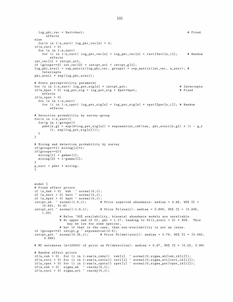
101
log_phi_vec = Xavl*bavl; # Fixed
effects
else
for(s in 1: n_surv) log_phi_vec[s] = 0;
if(n_ravl > 0)
for (s in 1: n_surv)
for (i in 1: n_ravl) log_phi_vec[s] = log_phi_vec[s] + ravl[Zavl[s,i]]; # Random
effects
int_vec [1] = intcpt_avl;
if (groups ==2) int_vec [2] = intcpt_avl + intcpt_g [1];
log_phi_avail = rep_matrix(log_phi_vec , groups) + rep_matrix(int_vec , n_surv); #
Intercepts
phi_avail = exp(log_phi_avail);
# State perceptibility parameter
for (s in 1: n_surv) log_pst_sig[s] = intcpt_pst; # Intercepts
if(n_bpst > 0) log_pst_sig = log_pst_sig + Xpst*bpst; # Fixed
effects
if(n_rpst > 0)
for (s in 1: n_surv)
for (i in 1: n_rpst) log_pst_sig[s] = log_pst_sig[s] + rpst[Zpst[s,i]]; # Random
effects
# Detection probability by survey -group
for(s in 1: n_surv){
for(g in 1: groups){
pdet[s,g] = exp(2* log_pst_sig[s]) * exponential_cdf(tau , phi_avail[s,g]) * (1 - g_r
(1, exp(log_pst_sig[s])));
}
}
# Mixing and detection probability by survey
if(groups ==1) mixing [1]=1;
if(groups ==2){
mixing [1] = gamma [1];
mixing [2] = 1-gamma [1];
}
p_surv = pdet * mixing;
}
model {
# Fixed effect priors
if (n_bab > 0) bab ~ normal (0,1);
if (n_bavl > 0) bavl ~ normal (0,1);
if (n_bpst > 0) bpst ~ normal (0,1);
intcpt_ab ~ normal (1.5 ,1); # Prior expected abundance: median = 4.48, 95% CI =
(0.631 , 31.8)
intcpt_avl ~ normal (-1.8,1); # Prior Pr(avail): median = 0.809, 95% CI = (0.208 ,
1.00)
# Below ~30% availability , binomial abundance models are unreliable.
# At upper end of CI , phi = 1.17, leading to Pr(t_avail < 2) = 90%. This
may be low for some species ,
# but if that is the case , then non -availability is not an issue.
if (groups ==2) intcpt_g ~ exponential (0.5);
intcpt_pst ~ normal (0.35 ,1); # Prior Pr(det|avail): median = 0.79, 95% CI = (0.040 ,
0.995)
# MC estimates (n=10000) of prior on Pr(detection): median = 0.47, 95% CI = (0.02, 0.98)
# Random effect priors
if(n_rab > 0) for (i in 1:sum(n_rabs)) rab[i] ~ normal(0,sigma_ab[vab_id[i]]);
if(n_ravl > 0) for (i in 1:sum(n_ravls)) ravl[i] ~ normal(0,sigma_avl[vavl_id[i]]);
if(n_rpst > 0) for (i in 1:sum(n_rpsts)) rpst[i] ~ normal(0,sigma_pst[vpst_id[i]]);
if(n_rab > 0) sigma_ab ~ cauchy (0,1);
if(n_ravl > 0) sigma_avl ~ cauchy (0,1);

102
if(n_rpst > 0) sigma_pst ~ cauchy (0,1);
# Other parameter priors
if (groups ==2) gamma ~ beta (1,1);
# Data models
n_bysurv ~ poisson_log(log(p_surv) + log_lambda);
# Increment the log -likelihood for the joint distribution of (r,t):
for(b in 1: n_bird){ # log(f_{r,t}|det) = log(f_r|det) + log(f_t|det) in this
model
# log(f_r|det) = log(2r/w^2 * g(r)) = constant + log(r) + log(g(r))
target += log(dist_obs[b]) +
log(g_r(dist_obs[b], exp(log_pst_sig[surv_obs[b]])*maxdist));
}
if (groups ==2) for(b in 1: n_bird){
# f_t|det = [gamma*dexp(t,phi1) + (1-gamma)*dexp(t,phi2)] / pdet
target += log(mixing [1] * exp(exponential_lpdf(time_obs[b] | phi_avail[surv_obs[b],1])
) +
mixing [2] * exp(exponential_lpdf(time_obs[b] | phi_avail[surv_obs[b],2])
)) -
log(p_surv[surv_obs[b]]);
}
if (groups ==1) for(b in 1: n_bird){
target += exponential_lpdf(time_obs[b] | phi_avail[surv_obs[b],1]) -
log(p_surv[surv_obs[b]]);
}
}
generated quantities {
int <lower=0> unobserved[n_surv ]; # Sampled uncounted birds
int <lower=0> totN[n_surv ]; # Sampled total birds
real <lower=0,upper=1> global_p; # Sampled overall detection probability
vector <upper =0>[ n_surv] log_lik; # LogLikelhood for LOO / WAIC calculations. Survey
is the observational unit.
# Surprisingly , neither TotN nor global_p can be vectorized:
for (s in 1: n_surv) {
unobserved[s] = poisson_rng(exp(log_lambda[s] + log(1-p_surv[s]))); # Uncounted ~ Po(\
lambda *(1-p))
totN[s] = n_bysurv[s] + unobserved[s];
log_lik[s] = poisson_log_lpmf(n_bysurv[s] | log(p_surv[s]) + log_lambda[s]);
}
# Calculate log -likelihood for (n, r, t | \lambda , \varphi , \sigma)... same as above
if(groups ==2) for(b in 1: n_bird){
log_lik[surv_obs[b]] = log_lik[surv_obs[b]] + log(2) - 2*log(maxdist) +
log(dist_obs[b]) + log(g_r(dist_obs[b], exp(log_pst_sig[surv_obs[b]])*
maxdist)) +
log(mixing [1] * exp(exponential_lpdf(time_obs[b] | phi_avail[surv_obs[b
],1])) +
mixing [2] * exp(exponential_lpdf(time_obs[b] | phi_avail[surv_obs[b
],2]))) -
log(p_surv[surv_obs[b]]);
}
if(groups ==1) for(b in 1: n_bird){
log_lik[surv_obs[b]] = log_lik[surv_obs[b]] + log(2) - 2*log(maxdist) +
log(dist_obs[b]) + log(g_r(dist_obs[b], exp(log_pst_sig[surv_obs[b]])*
maxdist)) +
exponential_lpdf(time_obs[b] | phi_avail[surv_obs[b],1]) -
log(p_surv[surv_obs[b]]);
}
# This calculation is split into 2 pieces , because of integers , reals , and the C++
oddity that: int/int = int
global_p = sum(n_bysurv);
global_p = global_p / sum(totN);
103
// totN[s] = n_bysurv[s] + unobserved[s];
// for (i in 1: n_ints) {
// yrep[s,i] = poisson_rng(exp(log_mu_ab[ii[s]+i]));
// p_int[i] = exp(log_p[s,i]); # Estimated p[s,i]
// lpn_BK[s,i] = poisson_log(y[s,i], exp(log_mu_ab[ii[s]+i]));
// dev1 = dev1 - 2 * lpn_BK[s,i];
// }
}

104
Event Model
##### Outstanding Issues:
functions{
# This code fits the exponential integral aka E1().
# Code is adapted from "Numerical Recipes in C", chapter 6.3:
# http :// www.aip.de/groups/soe/local/numres/bookcpdf/c6 -3.pdf
real E1(real x){
int MAXIT;
real a;
real b;
real c;
real d;
real del;
real fact;
real h;
real ans;
real EULER;
real EPS;
real FPMIN;
EULER =0.57721566490153286060651209008240243104215933593992;
MAXIT =100;
FPMIN =1.0e-30;
EPS =1.0e-7;
if (x < 0.0 || (x==0.0)){
reject ("Bad arguments in expint ");
} else {
if (x > 1.0) {
b = x+1.0;
c = 1.0/ FPMIN;
d = 1.0/b;
h = d;
for (i in 1:MAXIT){
a = -i*(i);
b = b+2.0;
d = 1.0/(a*d+b);
c = b+a/c;
del = c*d;
h = h*del;
if (fabs(del -1.0) < EPS) {
ans=h*exp(-x);
return ans;
}
}
reject (" Continued fraction failed in expint ");
} else {
ans = -log(x)-EULER; // Set first term.
fact = 1.0;
for (i in 1:MAXIT){
fact = -(x/i)*fact;
del = -fact/i;
ans = ans + del;
if (fabs(del) < fabs(ans)*EPS) return ans;
}
reject (" Series failed in expint ");
}
}
return ans;
}
real g_r(real r, real sigma){
return exp(-(r/sigma)^2);
}
}
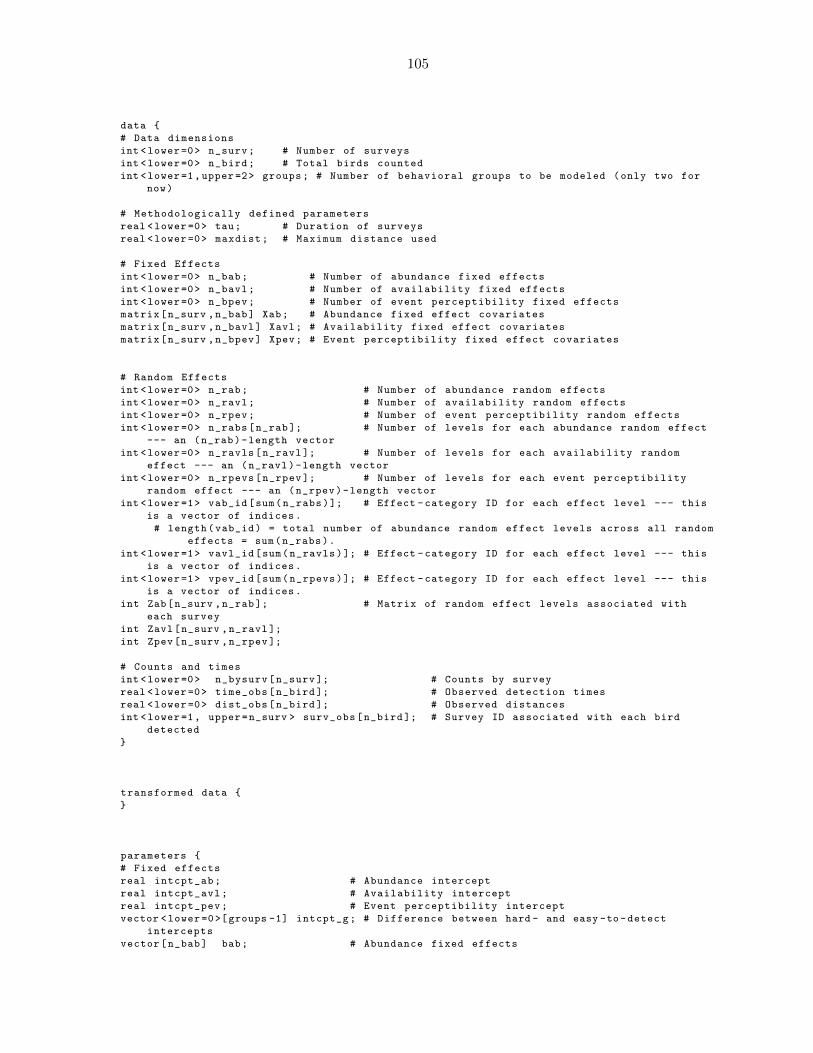
105
data {
# Data dimensions
int <lower=0> n_surv; # Number of surveys
int <lower=0> n_bird; # Total birds counted
int <lower=1,upper=2> groups; # Number of behavioral groups to be modeled (only two for
now)
# Methodologically defined parameters
real <lower=0> tau; # Duration of surveys
real <lower=0> maxdist; # Maximum distance used
# Fixed Effects
int <lower=0> n_bab; # Number of abundance fixed effects
int <lower=0> n_bavl; # Number of availability fixed effects
int <lower=0> n_bpev; # Number of event perceptibility fixed effects
matrix[n_surv ,n_bab] Xab; # Abundance fixed effect covariates
matrix[n_surv ,n_bavl] Xavl; # Availability fixed effect covariates
matrix[n_surv ,n_bpev] Xpev; # Event perceptibility fixed effect covariates
# Random Effects
int <lower=0> n_rab; # Number of abundance random effects
int <lower=0> n_ravl; # Number of availability random effects
int <lower=0> n_rpev; # Number of event perceptibility random effects
int <lower=0> n_rabs[n_rab ]; # Number of levels for each abundance random effect
--- an (n_rab)-length vector
int <lower=0> n_ravls[n_ravl ]; # Number of levels for each availability random
effect --- an (n_ravl)-length vector
int <lower=0> n_rpevs[n_rpev ]; # Number of levels for each event perceptibility
random effect --- an (n_rpev)-length vector
int <lower=1> vab_id[sum(n_rabs)]; # Effect -category ID for each effect level --- this
is a vector of indices.
# length(vab_id) = total number of abundance random effect levels across all random
effects = sum(n_rabs).
int <lower=1> vavl_id[sum(n_ravls)]; # Effect -category ID for each effect level --- this
is a vector of indices.
int <lower=1> vpev_id[sum(n_rpevs)]; # Effect -category ID for each effect level --- this
is a vector of indices.
int Zab[n_surv ,n_rab ]; # Matrix of random effect levels associated with
each survey
int Zavl[n_surv ,n_ravl ];
int Zpev[n_surv ,n_rpev ];
# Counts and times
int <lower=0> n_bysurv[n_surv ]; # Counts by survey
real <lower=0> time_obs[n_bird ]; # Observed detection times
real <lower=0> dist_obs[n_bird ]; # Observed distances
int <lower=1, upper=n_surv > surv_obs[n_bird ]; # Survey ID associated with each bird
detected
}
transformed data {
}
parameters {
# Fixed effects
real intcpt_ab; # Abundance intercept
real intcpt_avl; # Availability intercept
real intcpt_pev; # Event perceptibility intercept
vector <lower =0>[groups -1] intcpt_g; # Difference between hard - and easy -to-detect
intercepts
vector[n_bab] bab; # Abundance fixed effects

106
vector[n_bavl] bavl; # Availability fixed effects
vector[n_bpev] bpev; # Event perceptibility fixed effects
# Random effects
vector <lower =0>[n_rab] sigma_ab; # Abundance random effect standard deviation(s)
vector <lower =0>[ n_ravl] sigma_avl; # Availability random effect standard deviation(s)
vector <lower =0>[ n_rpev] sigma_pev; # Event perceptibility random effect standard
deviation(s)
vector[sum(n_rabs)] rab; # Vector of estimated abundance random effects for
all levels
vector[sum(n_ravls)] ravl; # Vector of estimated availability random effects for
all levels
vector[sum(n_rpevs)] rpev; # Vector of estimated event perceptibility random
effects for all levels
# Other parameters
vector <lower=0,upper=1>[groups -1] gamma; # Mixing parameter. gamma = hard -to-detect , (1-
gamma) = easy -to -detect
}
transformed parameters {
vector[n_surv] log_lambda; # log(expected survey abundance)
vector[n_surv] log_phi_vec; # log(fixed and random effects on
availability ... ignores intercepts , which vary by group)
matrix[n_surv ,groups] log_phi_avail; # log(survey availability rate parameter)
for each group
vector[n_surv] log_pev_sig; # log(distance parameter)
# If we have individual -level random effects , it may be necessary to define a survey -
level rate parameter
matrix <lower =0>[n_surv ,groups] phi_avail; # Survey availability rate parameter
matrix <lower=0, upper=1>[n_surv ,groups] pdet; # Probability of detection by survey x
group
vector <lower=0, upper=1>[ n_surv] p_surv; # Probability of detection by survey
across groups
vector <lower=0, upper=1>[ groups] mixing; # Mixing vector , sums to 1
row_vector[groups] int_vec; # Vector of detection intercepts
# Expected abundance
for (s in 1: n_surv) log_lambda[s] = intcpt_ab; # Intercepts
if(n_bab > 0) log_lambda = log_lambda + Xab*bab; # Fixed effects
if(n_rab > 0)
for (s in 1: n_surv)
for (i in 1:n_rab) log_lambda[s] = log_lambda[s] + rab[Zab[s,i]]; # Random effects
# Availability rate
if(n_bavl > 0)
log_phi_vec = Xavl*bavl; # Fixed
effects
else
for(s in 1: n_surv) log_phi_vec[s] = 0;
if(n_ravl > 0)
for (s in 1: n_surv)
for (i in 1: n_ravl) log_phi_vec[s] = log_phi_vec[s] + ravl[Zavl[s,i]]; # Random
effects
int_vec [1] = intcpt_avl;
if (groups ==2) int_vec [2] = intcpt_avl + intcpt_g [1];
log_phi_avail = rep_matrix(log_phi_vec , groups) + rep_matrix(int_vec , n_surv); #
Intercepts
phi_avail = exp(log_phi_avail);
# Event perceptibility parameter
for (s in 1: n_surv) log_pev_sig[s] = intcpt_pev; # Intercepts
if(n_bpev > 0) log_pev_sig = log_pev_sig + Xpev*bpev; # Fixed
effects
if(n_rpev > 0)

107
for (s in 1: n_surv)
for (i in 1: n_rpev) log_pev_sig[s] = log_pev_sig[s] + rpev[Zpev[s,i]]; # Random
effects
# Detection probability by survey -group
for(s in 1: n_surv){
for(g in 1: groups){
pdet[s,g] = 1 + exp(2* log_pev_sig[s]) * (E1(phi_avail[s,g]*tau) - E1(phi_avail[s,g]*
tau*g_r(1, exp(log_pev_sig[s]))));
}
}
# Mixing and detection probability by survey
if(groups ==1) mixing [1]=1;
if(groups ==2){
mixing [1] = gamma [1];
mixing [2] = 1-gamma [1];
}
p_surv = pdet * mixing;
}
model {
# Fixed effect priors
if (n_bab > 0) bab ~ normal (0,1);
if (n_bavl > 0) bavl ~ normal (0,1);
if (n_bpev > 0) bpev ~ normal (0,1);
intcpt_ab ~ normal (1.5 ,1); # Prior expected abundance: median = 4.48, 95% CI =
(0.631 , 31.8)
intcpt_avl ~ normal (-1.8,1); # Prior Pr(avail): median = 0.809, 95% CI = (0.208 ,
1.00)
# Below ~30% availability , binomial abundance models are unreliable.
# At upper end of CI , phi = 1.17, leading to Pr(t_avail < 2) = 90%. This
may be low for some species ,
# but if that is the case , then non -availability is not an issue.
if (groups ==2) intcpt_g ~ exponential (0.5);
intcpt_pev ~ normal (0.35 ,1); # Prior Pr(det|avail): median = 0.79, 95% CI = (0.040 ,
0.995)
# MC estimates (n=10000) of prior on Pr(detection): median = 0.58, 95% CI = (0.02, 1.00)
# Random effect priors
if(n_rab > 0) for (i in 1:sum(n_rabs)) rab[i] ~ normal(0,sigma_ab[vab_id[i]]);
if(n_ravl > 0) for (i in 1:sum(n_ravls)) ravl[i] ~ normal(0,sigma_avl[vavl_id[i]]);
if(n_rpev > 0) for (i in 1:sum(n_rpevs)) rpev[i] ~ normal(0,sigma_pev[vpev_id[i]]);
if(n_rab > 0) sigma_ab ~ cauchy (0,1);
if(n_ravl > 0) sigma_avl ~ cauchy (0,1);
if(n_rpev > 0) sigma_pev ~ cauchy (0,1);
# Other parameter priors
if (groups ==2) gamma ~ beta (1,1);
# Data models
n_bysurv ~ poisson_log(log(p_surv) + log_lambda);
# Increment the log -likelihood for the joint distribution of (r,t):
if(groups ==2) for(b in 1: n_bird){ # See the first section of derivations.pdf for the
exposition of this beastly equation
target += log(dist_obs[b]) +
log(mixing [1]* exp(exponential_lpdf(time_obs[b] | g_r(dist_obs[b],exp(
log_pev_sig[surv_obs[b]])*maxdist)*phi_avail[surv_obs[b],1])) +
mixing [2]* exp(exponential_lpdf(time_obs[b] | g_r(dist_obs[b],exp(
log_pev_sig[surv_obs[b]])*maxdist)*phi_avail[surv_obs[b],2]))) -
log(p_surv[surv_obs[b]]);
}
if(groups ==1) for(b in 1: n_bird){ # See the first section of derivations.pdf for the
exposition of this beastly equation

108
target += log(dist_obs[b]) +
exponential_lpdf(time_obs[b] | g_r(dist_obs[b],exp(log_pev_sig[surv_obs[b]])
*maxdist)*phi_avail[surv_obs[b],1]) -
log(p_surv[surv_obs[b]]);
}
}
generated quantities {
int <lower=0> unobserved[n_surv ]; # Sampled uncounted birds
int <lower=0> totN[n_surv ]; # Sampled total birds
real <lower=0,upper=1> global_p; # Sampled overall detection probability
vector <upper =0>[ n_surv] log_lik; # LogLikelhood for LOO / WAIC calculations. Survey
is the observational unit.
# Surprisingly , neither TotN nor global_p can be vectorized:
for (s in 1: n_surv) {
unobserved[s] = poisson_rng(exp(log_lambda[s] + log(1-p_surv[s]))); # Uncounted ~ Po(\
lambda *(1-p))
totN[s] = n_bysurv[s] + unobserved[s];
log_lik[s] = poisson_log_lpmf(n_bysurv[s] | log(p_surv[s]) + log_lambda[s]);
}
# Calculate log -likelihood for (n, r, t | \lambda , \varphi , \sigma)... same as above
if(groups ==2) for(b in 1: n_bird){
log_lik[surv_obs[b]] = log_lik[surv_obs[b]] + log(2) - 2*log(maxdist) + log(dist_obs[b
]) +
log(mixing [1]* exp(exponential_lpdf(time_obs[b] | g_r(dist_obs[b],exp(
log_pev_sig[surv_obs[b]])*maxdist)*phi_avail[surv_obs[b],1])) +
mixing [2]* exp(exponential_lpdf(time_obs[b] | g_r(dist_obs[b],exp(
log_pev_sig[surv_obs[b]])*maxdist)*phi_avail[surv_obs[b],2]))) -
log(p_surv[surv_obs[b]]);
}
if(groups ==1) for(b in 1: n_bird){
log_lik[surv_obs[b]] = log_lik[surv_obs[b]] + log(2) - 2*log(maxdist) + log(dist_obs[b
]) +
exponential_lpdf(time_obs[b] | g_r(dist_obs[b],exp(log_pev_sig[surv_obs[b
]])*maxdist)*phi_avail[surv_obs[b],1]) -
log(p_surv[surv_obs[b]]);
}
# This calculation is split into 2 pieces , because of integers , reals , and the C++
oddity that: int/int = int
global_p = sum(n_bysurv);
global_p = global_p / sum(totN);
// for (i in 1: n_ints) {
// yrep[s,i] = poisson_rng(exp(log_mu_ab[ii[s]+i]));
// p_int[i] = exp(log_p[s,i]); # Estimated p[s,i]
// lpn_BK[s,i] = poisson_log(y[s,i], exp(log_mu_ab[ii[s]+i]));
// dev1 = dev1 - 2 * lpn_BK[s,i];
// }
}

109
Combined Model
##### Outstanding Issues:
functions{
# Perceptibility function
real g_r(real r, real sigma){
return exp(-(r/sigma)^2);
}
# Pr(detection) involves an integral that can only be approximated by an infinite sum
# ’eval_int ’ evaluates that integral at one bound of integration
# a = 1/ sigma_pst ... NOT sigma_pst ^2
# b = phi*tau (where tau = C = duration of survey)
# c = 1/ sigma_pev ... NOT sigma_pev ^2
# Code adapted from Derivations.pdf
real eval_int(real r, real a, real b, real c){
int MAXIT;
real eaebc;
real denom;
real EPS; # Tolerance
real psumj; # Partial sum through j terms
real summand;
MAXIT =50;
denom = 1;
eaebc = - 0.5 * exp(-(a*r)^2) * exp(-b*exp(-(c*r)^2));
EPS = fabs (1.0e-15 / eaebc);
psumj = 0.0;
for (j in 0:MAXIT){
denom = denom * (a^2 + j*c^2);
summand = (b*c^2)^j * exp(-j*(c*r)^2) / denom;
psumj = psumj + summand;
if (fabs(summand) < EPS) return psumj * eaebc;
}
reject ("Error ");
return 99999; # Compiler wants to see a return statement , even though the ’reject ’
statement stops the code;
}
# Calculate pdet from the eval_int () function and equations derived in Derivations.pdf
real detcalc(real w, real a, real b, real c){
real ans;
ans = (a*w)^(-2)*(1.0-exp(-(a*w)^2)) - 2/(w^2) * (eval_int(w, a, b, c) - eval_int
(0.0, a, b, c));
return ans;
}
}
data {
# Data dimensions
int <lower=0> n_surv; # Number of surveys
int <lower=0> n_bird; # Total birds counted
int <lower=1,upper=2> groups; # Number of behavioral groups to be modeled (only two for
now)
# Methodologically defined parameters
real <lower=0> tau; # Duration of surveys
real <lower=0> maxdist; # Maximum distance used
# Fixed Effects
int <lower=0> n_bab; # Number of abundance fixed effects
int <lower=0> n_bavl; # Number of availability fixed effects
int <lower=0> n_bpev; # Number of event -perceptibility fixed effects
int <lower=0> n_bpst; # Number of state -perceptibility fixed effects
matrix[n_surv ,n_bab] Xab; # Abundance fixed effect covariates
matrix[n_surv ,n_bavl] Xavl; # Availability fixed effect covariates

110
matrix[n_surv ,n_bpev] Xpev; # Event -perceptibility fixed effect covariates
matrix[n_surv ,n_bpst] Xpst; # State -perceptibility fixed effect covariates
# Random Effects
int <lower=0> n_rab; # Number of abundance random effects
int <lower=0> n_ravl; # Number of availability random effects
int <lower=0> n_rpev; # Number of event -perceptibility random effects
int <lower=0> n_rpst; # Number of state -perceptibility random effects
int <lower=0> n_rabs[n_rab ]; # Vector of numbers of levels for each abundance
random effect
int <lower=0> n_ravls[n_ravl ]; # Vector of numbers of levels for each
availability random effect
int <lower=0> n_rpevs[n_rpev ]; # Vector of numbers of levels for each
perceptibility random effect
int <lower=0> n_rpsts[n_rpst ]; # Vector of numbers of levels for each
perceptibility random effect
int <lower=1> vab_id[sum(n_rabs)]; # Effect -category ID for each effect level ---
this is a vector of indices.
# length(vab_id) = total number of abundance random effect levels across all random
effects = sum(n_rabs).
int <lower=1> vavl_id[sum(n_ravls)]; # Effect -category ID for each effect level ---
this is a vector of indices.
int <lower=1> vpev_id[sum(n_rpevs)]; # Effect -category ID for each effect level --- this
is a vector of indices.
int <lower=1> vpst_id[sum(n_rpsts)]; # Effect -category ID for each effect level --- this
is a vector of indices.
int Zab[n_surv ,n_rab ]; # Matrix of random effect levels associated with
each survey
int Zavl[n_surv ,n_ravl ];
int Zpev[n_surv ,n_rpev ];
int Zpst[n_surv ,n_rpst ];
# Counts and times
int <lower=0> n_bysurv[n_surv ]; # Counts by survey
real <lower=0> time_obs[n_bird ]; # Observed detection times
real <lower=0> dist_obs[n_bird ]; # Observed distances
int <lower=1, upper=n_surv > surv_obs[n_bird ]; # Survey ID associated with each bird
detected
}
transformed data {
}
parameters {
# Fixed effects
real intcpt_ab; # Abundance intercept
real intcpt_avl; # Availability intercept
real intcpt_pev; # Event -perceptibility intercept
real intcpt_pst; # State -perceptibility intercept
vector <lower =0>[groups -1] intcpt_g; # Difference between hard - and easy -to-detect
intercepts
vector[n_bab] bab; # Abundance fixed effects
vector[n_bavl] bavl; # Availability fixed effects
vector[n_bpev] bpev; # Event -perceptibility fixed effects
vector[n_bpst] bpst; # State -perceptibility fixed effects
# Random effects
vector <lower =0>[n_rab] sigma_ab; # Abundance random effect standard deviation(s)
vector <lower =0>[ n_ravl] sigma_avl; # Availability random effect standard deviation(s)
vector <lower =0>[ n_rpev] sigma_pev; # Event -perceptibility random effect standard
deviation(s)
vector <lower =0>[ n_rpst] sigma_pst; # State -perceptibility random effect standard
deviation(s)

111
vector[sum(n_rabs)] rab; # Vector of estimated abundance random effects for
all levels
vector[sum(n_ravls)] ravl; # Vector of estimated availability random effects for
all levels
vector[sum(n_rpevs)] rpev; # Vector of estimated event -perceptibility random
effects for all levels
vector[sum(n_rpsts)] rpst; # Vector of estimated state -perceptibility random
effects for all levels
# Other parameters
vector <lower=0,upper=1>[groups -1] gamma; # Mixing parameter. gamma = hard -to-detect , (1-
gamma) = easy -to -detect
}
transformed parameters {
vector[n_surv] log_lambda; # log(expected survey abundance)
vector[n_surv] log_phi_vec; # log(fixed and random effects on
availability ... ignores intercepts , which vary by group)
matrix[n_surv ,groups] log_phi_avail; # log(survey availability rate parameter)
for each group
vector[n_surv] log_pev_sig; # log(event distance parameter)
vector[n_surv] log_pst_sig; # log(state distance parameter)
# If we have individual -level random effects , it may be necessary to define a survey -
level rate parameter
matrix <lower =0>[n_surv ,groups] phi_avail; # Survey availability rate parameter
matrix <lower=0, upper=1>[n_surv ,groups] pdet; # Probability of detection by survey x
group
vector <lower=0, upper=1>[ n_surv] p_surv; # Probability of detection by survey
across groups
vector <lower=0, upper=1>[ groups] mixing; # Mixing vector , sums to 1
row_vector[groups] int_vec; # Vector of detection intercepts
# Expected abundance
for (s in 1: n_surv) log_lambda[s] = intcpt_ab; # Intercepts
if(n_bab > 0) log_lambda = log_lambda + Xab*bab; # Fixed effects
if(n_rab > 0)
for (s in 1: n_surv)
for (i in 1:n_rab) log_lambda[s] = log_lambda[s] + rab[Zab[s,i]]; # Random effects
# Availability rate
if(n_bavl > 0)
log_phi_vec = Xavl*bavl; # Fixed
effects
else
for(s in 1: n_surv) log_phi_vec[s] = 0;
if(n_ravl > 0)
for (s in 1: n_surv)
for (i in 1: n_ravl) log_phi_vec[s] = log_phi_vec[s] + ravl[Zavl[s,i]]; # Random
effects
int_vec [1] = intcpt_avl;
if (groups ==2) int_vec [2] = intcpt_avl + intcpt_g [1];
log_phi_avail = rep_matrix(log_phi_vec , groups) + rep_matrix(int_vec , n_surv); #
Intercepts
phi_avail = exp(log_phi_avail);
# Event perceptibility parameter
for (s in 1: n_surv) log_pev_sig[s] = intcpt_pev; # Intercepts
if(n_bpev > 0) log_pev_sig = log_pev_sig + Xpev*bpev; # Fixed
effects
if(n_rpev > 0)
for (s in 1: n_surv)
for (i in 1: n_rpev) log_pev_sig[s] = log_pev_sig[s] + rpev[Zpev[s,i]]; # Random
effects
# State perceptibility parameter

112
for (s in 1: n_surv) log_pst_sig[s] = intcpt_pst; # Intercepts
if(n_bpst > 0) log_pst_sig = log_pst_sig + Xpst*bpst; # Fixed
effects
if(n_rpst > 0)
for (s in 1: n_surv)
for (i in 1: n_rpst) log_pst_sig[s] = log_pst_sig[s] + rpst[Zpst[s,i]]; # Random
effects
# Detection probability by survey -group
for(s in 1: n_surv){
for(g in 1: groups){
pdet[s,g] = detcalc(1, exp(-log_pst_sig[s]), tau*phi_avail[s,g], exp(-log_pev_sig[s
]));
# Function call: detcalc(real w, real a, real b, real c)
# a = 1/ sigma_s = exp(-log_pst_sig)
# b = phi*tau (where tau = C = duration of survey)
# c = 1/ sigma_e = exp(-log_pev_sig)
}
}
# Mixing and detection probability by survey
if(groups ==1) mixing [1]=1;
if(groups ==2){
mixing [1] = gamma [1];
mixing [2] = 1-gamma [1];
}
p_surv = pdet * mixing;
}
model {
# Fixed effect priors
if (n_bab > 0) bab ~ normal (0,1);
if (n_bavl > 0) bavl ~ normal (0,1);
if (n_bpev > 0) bpev ~ normal (0,1);
if (n_bpst > 0) bpst ~ normal (0,1);
intcpt_ab ~ normal (1.5 ,1); # Prior expected abundance: median = 4.48, 95% CI =
(0.631 , 31.8)
intcpt_avl ~ normal (-1.8,1); # Prior Pr(avail): median = 0.809, 95% CI = (0.208 ,
1.00)
# Below ~30% availability , binomial abundance models are unreliable.
# At upper end of CI , phi = 1.17, leading to Pr(t_avail < 2) = 90%. This
may be low for some species ,
# but if that is the case , then non -availability is not an issue.
if (groups ==2) intcpt_g ~ exponential (0.5);
intcpt_pev ~ normal (0.35 ,1); # Prior Pr(det|avail): median = 0.79, 95% CI = (0.040 ,
0.995)
intcpt_pst ~ normal (0.35 ,1); # Prior Pr(det|avail): median = 0.79, 95% CI = (0.040 ,
0.995)
# MC estimates (n=10000) of prior on Pr(detection): median = 0.35, 95% CI = (0.015 ,
0.95)
# Random effect priors
if(n_rab > 0) for (i in 1:sum(n_rabs)) rab[i] ~ normal(0,sigma_ab[vab_id[i]]);
if(n_ravl > 0) for (i in 1:sum(n_ravls)) ravl[i] ~ normal(0,sigma_avl[vavl_id[i]]);
if(n_rpev > 0) for (i in 1:sum(n_rpevs)) rpev[i] ~ normal(0,sigma_pev[vpev_id[i]]);
if(n_rpst > 0) for (i in 1:sum(n_rpsts)) rpst[i] ~ normal(0,sigma_pst[vpst_id[i]]);
if(n_rab > 0) sigma_ab ~ cauchy (0,1);
if(n_ravl > 0) sigma_avl ~ cauchy (0,1);
if(n_rpev > 0) sigma_pev ~ cauchy (0,1);
if(n_rpst > 0) sigma_pst ~ cauchy (0,1);
# Other parameter priors
if (groups ==2) gamma ~ beta (1,1);

113
# Data models
n_bysurv ~ poisson_log(log(p_surv) + log_lambda);
# Increment the log -likelihood for the joint distribution of (r,t):
if(groups ==2) for(b in 1: n_bird){ # See the third section of derivations.pdf for the
exposition
target += log(dist_obs[b]) +
log(g_r(dist_obs[b], exp(log_pst_sig[surv_obs[b]])*maxdist)) +
log(mixing [1]* exp(exponential_lpdf(time_obs[b] | g_r(dist_obs[b],exp(
log_pev_sig[surv_obs[b]])*maxdist)*phi_avail[surv_obs[b],1])) +
mixing [2]* exp(exponential_lpdf(time_obs[b] | g_r(dist_obs[b],exp(
log_pev_sig[surv_obs[b]])*maxdist)*phi_avail[surv_obs[b],2]))) -
log(p_surv[surv_obs[b]]);
}
if(groups ==1) for(b in 1: n_bird){
target += log(dist_obs[b]) +
log(g_r(dist_obs[b], exp(log_pst_sig[surv_obs[b]])*maxdist)) +
exponential_lpdf(time_obs[b] | g_r(dist_obs[b],exp(log_pev_sig[surv_obs[b]])
*maxdist)*phi_avail[surv_obs[b],1]) -
log(p_surv[surv_obs[b]]);
}
}
generated quantities {
int <lower=0> unobserved[n_surv ]; # Sampled uncounted birds
int <lower=0> totN[n_surv ]; # Sampled total birds
real <lower=0,upper=1> global_p; # Sampled overall detection probability
vector <upper =0>[ n_surv] log_lik; # LogLikelhood for LOO / WAIC calculations. Survey
is the observational unit.
# Surprisingly , neither TotN nor global_p can be vectorized:
for (s in 1: n_surv) {
unobserved[s] = poisson_rng(exp(log_lambda[s] + log(1-p_surv[s]))); # Uncounted ~ Po(\
lambda *(1-p))
totN[s] = n_bysurv[s] + unobserved[s];
log_lik[s] = poisson_log_lpmf(n_bysurv[s] | log(p_surv[s]) + log_lambda[s]);
}
# Calculate log -likelihood for (n, r, t | \lambda , \varphi , \sigma)... same as above
if(groups ==2) for(b in 1: n_bird){
log_lik[surv_obs[b]] = log_lik[surv_obs[b]] + log(2) - 2*log(maxdist) + log(dist_obs[b
]) +
log(g_r(dist_obs[b], exp(log_pst_sig[surv_obs[b]])*maxdist)) +
log(mixing [1]* exp(exponential_lpdf(time_obs[b] | g_r(dist_obs[b],exp(
log_pev_sig[surv_obs[b]])*maxdist)*phi_avail[surv_obs[b],1])) +
mixing [2]* exp(exponential_lpdf(time_obs[b] | g_r(dist_obs[b],exp(
log_pev_sig[surv_obs[b]])*maxdist)*phi_avail[surv_obs[b],2]))) -
log(p_surv[surv_obs[b]]);
}
if(groups ==1) for(b in 1: n_bird){
log_lik[surv_obs[b]] = log_lik[surv_obs[b]] + log(2) - 2*log(maxdist) + log(dist_obs[b
]) +
log(g_r(dist_obs[b], exp(log_pst_sig[surv_obs[b]])*maxdist)) +
exponential_lpdf(time_obs[b] | g_r(dist_obs[b],exp(log_pev_sig[surv_obs[b
]])*maxdist)*phi_avail[surv_obs[b],1]) -
log(p_surv[surv_obs[b]]);
}
# This calculation is split into 2 pieces , because of integers , reals , and the C++
oddity that: int/int = int
global_p = sum(n_bysurv);
global_p = global_p / sum(totN);
}

114
Supplementary tables and figures
pp = 0.4 pp = 0.65 pp = 0.83 pp = 0.98
●
●
●
●
●
●
●
●
●
●
●
●
●
●
●
●
●
●
●
●
●
●
●
●
●
●
●
●
●
●
●
●
●
●
●
●
●
●
●
●
●
●
●
●
●
●
●
●
●
●
●
●
●
●
●
●
●
●
●
●
●
●
●
●
●
●
●
●
●
●
●
●
●
●
Combined Model
Event Model
State Model
Combined Model
Event Model
State Model
Combined Model
Event Model
State Model
Combined Model
Event Model
State Model
Combined Model
Event Model
State Model
Combined Model
Event Model
State Model
Combined Model
Event Model
State Model
Combined Model
Event Model
State Model
Event
Event
Event
Event
State
State
State
State
pa =
0.4p
a =0.65
pa =
0.83p
a =0.98
pa =
0.4p
a =0.65
pa =
0.83p
a =0.98
0.00 0.25 0.50 0.75 1.000.00 0.25 0.50 0.75 1.000.00 0.25 0.50 0.75 1.000.00 0.25 0.50 0.75 1.00Posterior detection probability
Figure B.1 Caterpillar plot of posterior estimates for detection probability p(det) from a rep-resentative complete replicate set of simulations. Vertical gray bars show the truevalue, dots show the posterior median estimate, and horizontal lines show 95%credible intervals. Rows show the availability and model used in data simulation.Columns show the perceptibility used in data simulation.

115
Perceptibility
Event model State model Combined modelData Availability 0.40 0.65 0.83 0.98 0.40 0.65 0.83 0.98 0.40 0.65 0.98
Event
0.40 0.03 0.02 0.03 0.02 -0.04 -0.05 -0.02 -0.00 0.01 0.010.65 0.01 0.01 0.01 -0.01 -0.10 -0.12 -0.07 -0.040.83 -0.00 0.00 -0.00 0.00 -0.13 -0.15 -0.11 -0.03 -0.020.98 -0.00 0.00 -0.00 -0.00 -0.16 -0.18 -0.13 -0.04 -0.01 -0.03
State
0.40 0.06 0.08 0.06 0.01 0.01 0.01 0.01 -0.01 0.03 0.000.65 0.09 0.11 0.09 0.01 0.00 -0.00 0.01 -0.020.83 0.14 0.17 0.13 0.02 0.00 -0.00 0.02 -0.02 0.010.98 0.32 0.34 0.17 0.02 0.00 0.00 0.02 -0.01 0.00 -0.01
Table B.1 Bias of median posterior detection probability. Rows indicate the availability andmodel used for data simulation. Columns indicate the perceptibility used in datasimulation and the model used for inference. Total observations n(obs) = 800.
PerceptibilityEvent model State model Combined model
Data Availability 0.40 0.65 0.83 0.98 0.40 0.65 0.83 0.98 0.40 0.65 0.98
Eve
nt
0.40 52 56 54 34 16 22 46 48 62 420.65 34 52 44 56 0 0 20 440.83 36 46 32 48 0 0 6 42 460.98 40 42 42 40 0 0 0 2 30 2
Sta
te
0.40 20 34 52 42 56 34 46 46 41 500.65 2 6 12 40 38 48 42 440.83 0 0 0 42 46 48 60 48 400.98 0 0 0 0 38 50 44 64 38 66
Table B.2 Observed 50% coverage percentages for estimates of detection probability based on50 replicates with 800 observations per dataset. Rows indicate the availability andmodel used for data simulation. Columns indicate the perceptibility used in datasimulation and the model used for inference. Coverage values between (36, 64) arewithin a 95% confidence interval for nominal coverage.
Perceptibility
Event model State model Combined modelData Availability 0.40 0.65 0.83 0.98 0.40 0.65 0.83 0.98 0.40 0.65 0.98
Even
t
0.40 0.07 0.03 0.03 0.04 -0.09 -0.08 -0.03 0.02 0.03 0.030.65 0.01 0.00 0.00 0.00 -0.21 -0.17 -0.09 -0.020.83 -0.00 0.01 -0.01 0.01 -0.26 -0.20 -0.12 -0.01 -0.010.98 -0.00 -0.00 -0.00 -0.00 -0.22 -0.17 -0.11 -0.02 -0.01 -0.00
State
0.40 0.13 0.11 0.06 0.02 0.02 0.01 0.01 0.01 0.07 0.020.65 0.11 0.11 0.06 0.02 -0.01 -0.01 -0.00 -0.010.83 0.09 0.08 0.04 0.02 0.00 -0.00 0.00 0.00 0.020.98 0.01 0.00 0.00 0.00 0.00 -0.00 -0.00 -0.00 0.00 0.00
Table B.3 Bias of median posterior availability. The apparent disappearance of bias for eventmodels fit to state data at high availability reflects the fact there’s little room tobe biased when availability is already 98%. Rows indicate the availability andmodel used for data simulation. Columns indicate the perceptibility used in datasimulation and the model used for inference. Total observations n(obs) = 800.

116
pp = 0.4 pp = 0.65 pp = 0.83 pp = 0.98
●
●
●
●
●
●
●
●
●
●
●
●
●
●
●
●
●
●
●
●
●
●
●
●
●
●
●
●
●
●
●
●
●
●
●
●
●
●
●
●
●
●
●
●
●
●
●
●
●
●
●
●
●
●
●
●
●
●
●
●
●
●
●
●
●
●
●
●
●
●
●
●
●
●
Combined Model
Event Model
State Model
Combined Model
Event Model
State Model
Combined Model
Event Model
State Model
Combined Model
Event Model
State Model
Combined Model
Event Model
State Model
Combined Model
Event Model
State Model
Combined Model
Event Model
State Model
Combined Model
Event Model
State Model
Event
Event
Event
Event
State
State
State
State
pa =
0.4p
a =0.65
pa =
0.83p
a =0.98
pa =
0.4p
a =0.65
pa =
0.83p
a =0.98
0.25 0.50 0.75 1.00 0.25 0.50 0.75 1.00 0.25 0.50 0.75 1.00 0.25 0.50 0.75 1.00Posterior availability
Figure B.2 Caterpillar plot of posterior estimates for availability pa from a representativecomplete replicate set of simulations. Vertical gray bars show the true value,dots show the posterior median estimate, and horizontal lines show 95% credibleintervals. Rows show the availability and model used in data simulation. Columnsshow the perceptibility used in data simulation.
PerceptibilityEvent model State model Combined model
Data Availability 0.40 0.65 0.83 0.98 0.40 0.65 0.83 0.98 0.40 0.65 0.98
Eve
nt
0.40 50 46 42 28 20 24 46 38 62 320.65 38 56 40 62 0 0 10 480.83 40 44 52 44 0 0 0 56 600.98 30 52 50 54 0 0 0 0 36 58
Sta
te
0.40 22 34 48 38 56 38 54 44 45 380.65 12 8 24 50 46 46 52 460.83 0 2 18 38 46 50 54 48 360.98 6 36 40 38 42 36 34 48 42 36
Table B.4 Observed 50% coverage percentages for estimates of availability based on 50 repli-cates with 800 observations per dataset. Rows indicate the availability and modelused for data simulation. Columns indicate the perceptibility used in data simula-tion and the model used for inference. Coverage values between (36, 64) are withina 95% confidence interval for nominal coverage.
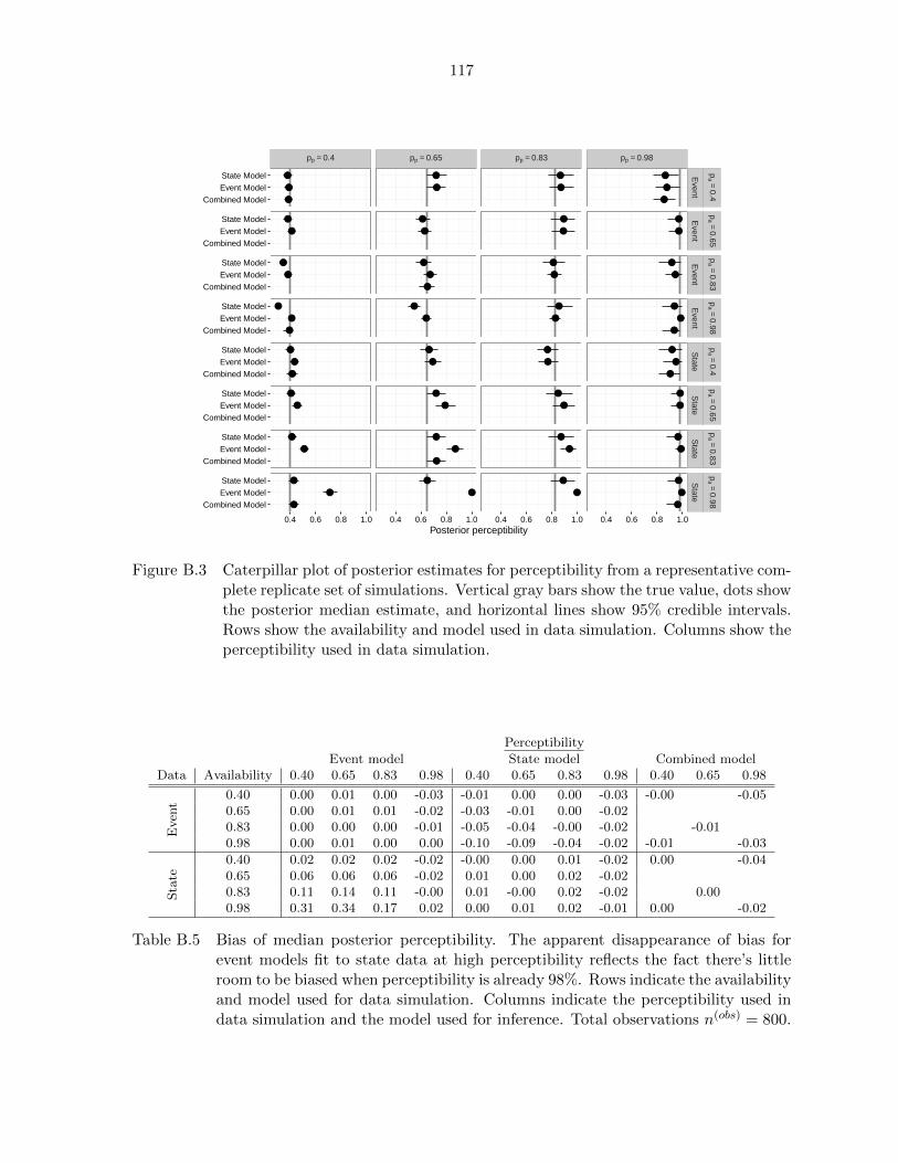
117
pp = 0.4 pp = 0.65 pp = 0.83 pp = 0.98
●
●
●
●
●
●
●
●
●
●
●
●
●
●
●
●
●
●
●
●
●
●
●
●
●
●
●
●
●
●
●
●
●
●
●
●
●
●
●
●
●
●
●
●
●
●
●
●
●
●
●
●
●
●
●
●
●
●
●
●
●
●
●
●
●
●
●
●
●
●
●
●
●
●
Combined Model
Event Model
State Model
Combined Model
Event Model
State Model
Combined Model
Event Model
State Model
Combined Model
Event Model
State Model
Combined Model
Event Model
State Model
Combined Model
Event Model
State Model
Combined Model
Event Model
State Model
Combined Model
Event Model
State Model
Event
Event
Event
Event
State
State
State
State
pa =
0.4p
a =0.65
pa =
0.83p
a =0.98
pa =
0.4p
a =0.65
pa =
0.83p
a =0.98
0.4 0.6 0.8 1.0 0.4 0.6 0.8 1.0 0.4 0.6 0.8 1.0 0.4 0.6 0.8 1.0Posterior perceptibility
Figure B.3 Caterpillar plot of posterior estimates for perceptibility from a representative com-plete replicate set of simulations. Vertical gray bars show the true value, dots showthe posterior median estimate, and horizontal lines show 95% credible intervals.Rows show the availability and model used in data simulation. Columns show theperceptibility used in data simulation.
Perceptibility
Event model State model Combined modelData Availability 0.40 0.65 0.83 0.98 0.40 0.65 0.83 0.98 0.40 0.65 0.98
Even
t
0.40 0.00 0.01 0.00 -0.03 -0.01 0.00 0.00 -0.03 -0.00 -0.050.65 0.00 0.01 0.01 -0.02 -0.03 -0.01 0.00 -0.020.83 0.00 0.00 0.00 -0.01 -0.05 -0.04 -0.00 -0.02 -0.010.98 0.00 0.01 0.00 0.00 -0.10 -0.09 -0.04 -0.02 -0.01 -0.03
State
0.40 0.02 0.02 0.02 -0.02 -0.00 0.00 0.01 -0.02 0.00 -0.040.65 0.06 0.06 0.06 -0.02 0.01 0.00 0.02 -0.020.83 0.11 0.14 0.11 -0.00 0.01 -0.00 0.02 -0.02 0.000.98 0.31 0.34 0.17 0.02 0.00 0.01 0.02 -0.01 0.00 -0.02
Table B.5 Bias of median posterior perceptibility. The apparent disappearance of bias forevent models fit to state data at high perceptibility reflects the fact there’s littleroom to be biased when perceptibility is already 98%. Rows indicate the availabilityand model used for data simulation. Columns indicate the perceptibility used indata simulation and the model used for inference. Total observations n(obs) = 800.

118
PerceptibilityEvent model State model Combined model
Data Availability 0.40 0.65 0.83 0.98 0.40 0.65 0.83 0.98 0.40 0.65 0.98E
vent
0.40 52 56 50 58 40 52 50 62 60 00.65 52 58 50 76 6 46 38 680.83 48 50 64 74 2 26 58 60 600.98 44 46 42 48 0 2 40 72 38 12
Sta
te
0.40 26 40 42 76 50 44 48 68 53 60.65 2 12 26 70 46 50 52 500.83 0 2 0 82 38 46 50 62 440.98 0 0 0 0 38 42 38 72 42 56
Table B.6 Observed 50% coverage percentages for estimates of perceptibility based on 50replicates with 800 observations per dataset. Rows indicate the availability andmodel used for data simulation. Columns indicate the perceptibility used in datasimulation and the model used for inference. Coverage values between (36, 64) arewithin a 95% confidence interval for nominal coverage.
pp = 0.4 pp = 0.65 pp = 0.83 pp = 0.98
●
●
●
●
●
●
●
●
●
●
●
●
●
●
●
●
●
●
●
●
400
800
400
800
400
800
400
800
400
800
400
800
400
800
400
800
Event
Event
Event
Event
State
State
State
State
pa =
0.4p
a =0.65
pa =
0.83p
a =0.98
pa =
0.4p
a =0.65
pa =
0.83p
a =0.98
−10 −5 0 −10 −5 0 −10 −5 0 −10 −5 0∆elpd / se(∆elpd)
Num
ber
of O
bser
vatio
ns
Figure B.4 Model comparisons between combined and true models in expected predictiveaccuracy (∆elpd) relative to the standard error of that difference. Dashed verticallines show 95% confidence intervals for the hypothesis that models are equallypredictive – i.e., ∆elpd is zero. Large dots shows the median value across allsimulated datasets, while horizontal lines show the central 90% quantiles.

119
PerceptibilityEvent model State model Combined model
Data Availability 0.40 0.65 0.83 0.98 0.40 0.65 0.83 0.98 0.40 0.65 0.98
Eve
nt
0.40 -18 -16 -10 -6 19 11 3 -0 -10 -20.65 -4 -0 2 5 55 35 17 120.83 3 1 -0 1 73 41 16 7 90.98 -1 -0 0 0 71 40 17 6 4 6
Sta
te
0.40 -30 -21 -13 -4 -9 -1 -2 2 -22 -10.65 -22 -20 -13 -1 4 0 -1 50.83 -28 -25 -15 -1 -0 -1 -2 6 -50.98 -48 -35 -17 -2 -2 -1 -4 3 -2 3
Table B.7 Percent bias of the median posterior expected abundance (calculated from log-scalebias averaged over 50 replicates). Rows indicate the availability and model usedfor data simulation. Columns indicate the perceptibility used in data simulationand the model used for inference. Total observations n(obs) = 400.
PerceptibilityEvent model State model Combined model
Data Availability 0.40 0.65 0.83 0.98 0.40 0.65 0.83 0.98 0.40 0.65 0.98
Eve
nt
0.40 50 48 52 54 38 50 50 46 64 500.65 48 58 46 50 0 8 30 400.83 56 54 44 78 0 0 28 42 480.98 56 54 72 100 0 0 8 16 54 20
Sta
te
0.40 24 36 48 44 54 40 56 56 40 520.65 16 16 24 52 54 40 58 520.83 0 0 2 70 56 52 54 58 460.98 0 0 0 100 54 50 54 82 54 82
Table B.8 Observed 50% coverage percentages for estimates of expected abundance based on50 replicates with 800 observations per dataset. Rows indicate the availability andmodel used for data simulation. Columns indicate the perceptibility used in datasimulation and the model used for inference. Coverage values between (36, 64) arewithin a 95% confidence interval for nominal coverage.

120
APPENDIX C. SUPPORTING FIGURES FOR CHAPTER 4
Supplementary figures
●
●
●
●
●
●
●
●
●
●
●
●
●
●
●
●
●
●
●
●
●
●
●
●
●
●
●
●
●
●
●
●
●
●
●
●
●
●
●
●
●
●
●
●
●
●
●
●
●
●
●
●
●
●
●
●
●
●
●
●
●
●
●
●
●
●
●
●
●
●
●
●
●
●
●
●
●
●
●
●
●
●
●
●
●
●
●
●
●
●
●
●
●
●
●
●
●
●
●
●
●
●
●
●
●
●
●
●
●
●
●
●
●
●
●
●
●
●
●
●
Density Pr(Detection) Availability Perceptibility
Red−
winged
blackirdK
illdeerE
asternm
eadowlark
Dickcissel
Com
mon
yellowthroat
Am
ericanrobin
40 80 120 0.2 0.4 0.6 0.2 0.4 0.6 0.80.2 0.4 0.6 0.8 1.0
99149174199224
99149174199224
99149174199224
99149174199224
99149174199224
99149174199224
Dis
tanc
e
Figure C.1 Posterior marginal estimates of abundance density (per km2), detection proba-bility, availability, and perceptibility. By definition, Pr(Detection) = availability× perceptibility. Black lines show 95% credible intervals, orange lines show 50%credible intervals, and black dots show posterior medians.

121
●
●
●
●
●
●
●
●
●
●
●
●
●
●
●
●
●
●
●
●
●
●
●
●
●
●
●
●
●
●
●
●
●
●
●
●
●
●
●
●
●
●
●
●
●
●
●
●
●
●
●
●
●
●
●
●
●
●
●
●
●
●
●
●
●
●
●
●
●
●
●
●
●
●
●
●
●
●
●
●
●
●
●
●
●
●
●
●
●
●
Event: Intercept Event: Wind State: Intercept
Avail: Mixing Avail: Time of Day Avail: Julian Date Avail: Cloud Cover Avail: Date StDev
Abund: Strips 2016 Abund: Location StDev Avail: Hard−to−Detect Avail: Easy−to−Detect Avail: Easy−Hard Diff
Abund: Control 2015 Abund: Proxy 2015 Abund: Strips 2015 Abund: Control 2016 Abund: Proxy 2016
1 2 3 −0.5 0.0 0.5 1.0 1.5 −0.5 0.0 0.5 1.0
0.4 0.5 0.6 0.7 0.8 −0.8 −0.4 0.0 0.4 −1.5 −1.0 −0.5 −0.75−0.50−0.250.00 0.25 0.0 0.5 1.0 1.5
−1.0 −0.5 0.0 0.5 0.4 0.6 0.8 1.0 1.2 −4 −3 −2 2 3 4 5 2 3 4 5
−1.0 −0.5 0.0 0.5 −0.5 0.0 0.5 1.0 −1.0 −0.5 0.0 0.5 −1.0 −0.5 0.0 0.5 −1.0 −0.5 0.0 0.5 1.0
99
149
174
199
224
99
149
174
199
224
99
149
174
199
224
99
149
174
199
224
99
149
174
199
224
99
149
174
199
224
99
149
174
199
224
99
149
174
199
224
99
149
174
199
224
99
149
174
199
224
99
149
174
199
224
99
149
174
199
224
99
149
174
199
224
99
149
174
199
224
99
149
174
199
224
99
149
174
199
224
99
149
174
199
224
99
149
174
199
224
Trun
catio
n D
ista
nce
American Robins
Figure C.2 Posterior parameter estimates. All estimates are on the log-scale for the appro-priate model component. Abundance: treatment-year effects plus random loca-tion-specific variability. Availability: availability rate intercepts for hard- andeasy-to-detect birds, their difference, and the mixing parameter γ giving the pro-portion of birds that are hard-to-detect; covariates for time of day, Julian date,and cloud cover; random day-to-day availability variability. Event perceptibility:intercept terms and a covariate for wind. State perceptibility: intercept term.Black lines show 95% credible intervals, orange lines show 50% credible intervals,and black dots show the posterior mean.
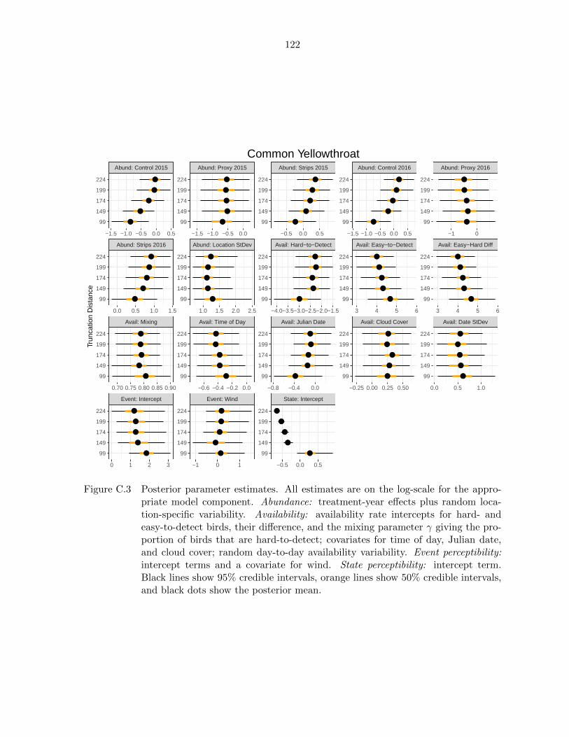
122
●
●
●
●
●
●
●
●
●
●
●
●
●
●
●
●
●
●
●
●
●
●
●
●
●
●
●
●
●
●
●
●
●
●
●
●
●
●
●
●
●
●
●
●
●
●
●
●
●
●
●
●
●
●
●
●
●
●
●
●
●
●
●
●
●
●
●
●
●
●
●
●
●
●
●
●
●
●
●
●
●
●
●
●
●
●
●
●
●
●
Event: Intercept Event: Wind State: Intercept
Avail: Mixing Avail: Time of Day Avail: Julian Date Avail: Cloud Cover Avail: Date StDev
Abund: Strips 2016 Abund: Location StDev Avail: Hard−to−Detect Avail: Easy−to−Detect Avail: Easy−Hard Diff
Abund: Control 2015 Abund: Proxy 2015 Abund: Strips 2015 Abund: Control 2016 Abund: Proxy 2016
0 1 2 3 −1 0 1 −0.5 0.0 0.5
0.70 0.75 0.80 0.85 0.90 −0.6 −0.4 −0.2 0.0 −0.8 −0.4 0.0 −0.25 0.00 0.25 0.50 0.0 0.5 1.0
0.0 0.5 1.0 1.5 1.0 1.5 2.0 2.5 −4.0−3.5−3.0−2.5−2.0−1.5 3 4 5 6 3 4 5 6
−1.5 −1.0 −0.5 0.0 0.5 −1.5 −1.0 −0.5 0.0 −0.5 0.0 0.5 −1.5 −1.0 −0.5 0.0 0.5 −1 0
99
149
174
199
224
99
149
174
199
224
99
149
174
199
224
99
149
174
199
224
99
149
174
199
224
99
149
174
199
224
99
149
174
199
224
99
149
174
199
224
99
149
174
199
224
99
149
174
199
224
99
149
174
199
224
99
149
174
199
224
99
149
174
199
224
99
149
174
199
224
99
149
174
199
224
99
149
174
199
224
99
149
174
199
224
99
149
174
199
224
Trun
catio
n D
ista
nce
Common Yellowthroat
Figure C.3 Posterior parameter estimates. All estimates are on the log-scale for the appro-priate model component. Abundance: treatment-year effects plus random loca-tion-specific variability. Availability: availability rate intercepts for hard- andeasy-to-detect birds, their difference, and the mixing parameter γ giving the pro-portion of birds that are hard-to-detect; covariates for time of day, Julian date,and cloud cover; random day-to-day availability variability. Event perceptibility:intercept terms and a covariate for wind. State perceptibility: intercept term.Black lines show 95% credible intervals, orange lines show 50% credible intervals,and black dots show the posterior mean.
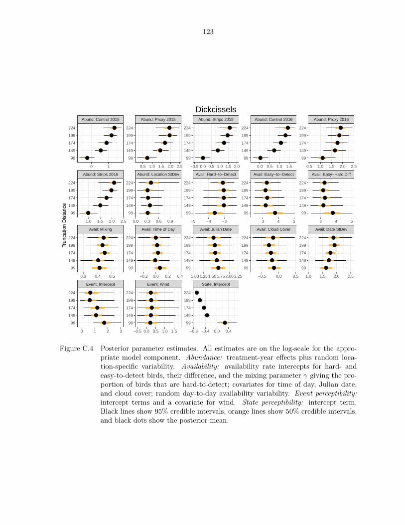
123
●
●
●
●
●
●
●
●
●
●
●
●
●
●
●
●
●
●
●
●
●
●
●
●
●
●
●
●
●
●
●
●
●
●
●
●
●
●
●
●
●
●
●
●
●
●
●
●
●
●
●
●
●
●
●
●
●
●
●
●
●
●
●
●
●
●
●
●
●
●
●
●
●
●
●
●
●
●
●
●
●
●
●
●
●
●
●
●
●
●
Event: Intercept Event: Wind State: Intercept
Avail: Mixing Avail: Time of Day Avail: Julian Date Avail: Cloud Cover Avail: Date StDev
Abund: Strips 2016 Abund: Location StDev Avail: Hard−to−Detect Avail: Easy−to−Detect Avail: Easy−Hard Diff
Abund: Control 2015 Abund: Proxy 2015 Abund: Strips 2015 Abund: Control 2016 Abund: Proxy 2016
0 1 2 3 −0.5 0.0 0.5 1.0 1.5 −0.8 −0.4 0.0 0.4
0.3 0.4 0.5 −0.2 0.0 0.2 0.4 1.00 1.25 1.50 1.75 2.00 2.25 −0.5 0.0 0.5 1.0 1.5 2.0 2.5
1.0 1.5 2.0 2.5 0.0 0.3 0.6 0.9 −5 −4 −3 3 4 5 3 4 5
0 1 0.5 1.0 1.5 2.0 2.5 −0.5 0.0 0.5 1.0 1.5 2.0 0.0 0.5 1.0 1.5 0.5 1.0 1.5 2.0 2.5
99
149
174
199
224
99
149
174
199
224
99
149
174
199
224
99
149
174
199
224
99
149
174
199
224
99
149
174
199
224
99
149
174
199
224
99
149
174
199
224
99
149
174
199
224
99
149
174
199
224
99
149
174
199
224
99
149
174
199
224
99
149
174
199
224
99
149
174
199
224
99
149
174
199
224
99
149
174
199
224
99
149
174
199
224
99
149
174
199
224
Trun
catio
n D
ista
nce
Dickcissels
Figure C.4 Posterior parameter estimates. All estimates are on the log-scale for the appro-priate model component. Abundance: treatment-year effects plus random loca-tion-specific variability. Availability: availability rate intercepts for hard- andeasy-to-detect birds, their difference, and the mixing parameter γ giving the pro-portion of birds that are hard-to-detect; covariates for time of day, Julian date,and cloud cover; random day-to-day availability variability. Event perceptibility:intercept terms and a covariate for wind. State perceptibility: intercept term.Black lines show 95% credible intervals, orange lines show 50% credible intervals,and black dots show the posterior mean.

124
●
●
●
●
●
●
●
●
●
●
●
●
●
●
●
●
●
●
●
●
●
●
●
●
●
●
●
●
●
●
●
●
●
●
●
●
●
●
●
●
●
●
●
●
●
●
●
●
●
●
●
●
●
●
●
●
●
●
●
●
●
●
●
●
●
●
●
●
●
●
●
●
●
●
●
●
●
●
●
●
●
●
●
●
●
●
●
●
●
●
Event: Intercept Event: Wind State: Intercept
Avail: Mixing Avail: Time of Day Avail: Julian Date Avail: Cloud Cover Avail: Date StDev
Abund: Strips 2016 Abund: Location StDev Avail: Hard−to−Detect Avail: Easy−to−Detect Avail: Easy−Hard Diff
Abund: Control 2015 Abund: Proxy 2015 Abund: Strips 2015 Abund: Control 2016 Abund: Proxy 2016
1 2 3 0 1 −0.50.0 0.5 1.0 1.5 2.0 2.5
0.4 0.6 0.8 −0.4 −0.2 0.0 0.2 0.4 −2.0 −1.5 −1.0 −0.25 0.00 0.25 0.50 0.0 0.5 1.0
−0.5 0.0 0.5 1.0 0.5 1.0 1.5 −4 −3 −2 1 2 3 4 5 1 2 3 4 5
−1.0 −0.5 0.0 0.5 0.0 0.5 1.0 −0.5 0.0 0.5 1.0 −1.5 −1.0 −0.5 0.0 0.5 −1 0
99
149
174
199
224
99
149
174
199
224
99
149
174
199
224
99
149
174
199
224
99
149
174
199
224
99
149
174
199
224
99
149
174
199
224
99
149
174
199
224
99
149
174
199
224
99
149
174
199
224
99
149
174
199
224
99
149
174
199
224
99
149
174
199
224
99
149
174
199
224
99
149
174
199
224
99
149
174
199
224
99
149
174
199
224
99
149
174
199
224
Trun
catio
n D
ista
nce
Eastern Meadowlarks
Figure C.5 Posterior parameter estimates. All estimates are on the log-scale for the appro-priate model component. Abundance: treatment-year effects plus random loca-tion-specific variability. Availability: availability rate intercepts for hard- andeasy-to-detect birds, their difference, and the mixing parameter γ giving the pro-portion of birds that are hard-to-detect; covariates for time of day, Julian date,and cloud cover; random day-to-day availability variability. Event perceptibility:intercept terms and a covariate for wind. State perceptibility: intercept term.Black lines show 95% credible intervals, orange lines show 50% credible intervals,and black dots show the posterior mean.

125
●
●
●
●
●
●
●
●
●
●
●
●
●
●
●
●
●
●
●
●
●
●
●
●
●
●
●
●
●
●
●
●
●
●
●
●
●
●
●
●
●
●
●
●
●
●
●
●
●
●
●
●
●
●
●
●
●
●
●
●
●
●
●
●
●
●
●
●
●
●
●
●
●
●
●
●
●
●
●
●
●
●
●
●
●
●
●
●
●
●
Event: Intercept Event: Wind State: Intercept
Avail: Mixing Avail: Time of Day Avail: Julian Date Avail: Cloud Cover Avail: Date StDev
Abund: Strips 2016 Abund: Location StDev Avail: Hard−to−Detect Avail: Easy−to−Detect Avail: Easy−Hard Diff
Abund: Control 2015 Abund: Proxy 2015 Abund: Strips 2015 Abund: Control 2016 Abund: Proxy 2016
0 1 2 0 1 −0.6 −0.4 −0.2 0.0
0.00 0.25 0.50 0.75 1.00 −0.5 0.0 −1.5 −1.0 −0.5 0.0 −1.0 −0.5 0.0 0.5 1.0 1.5 2.0 2.5 3.0
−1.0 −0.5 0.0 0.5 0.5 1.0 1.5 2.0 −4 −3 −2 0 1 2 3 4 0 1 2 3 4
−1.0 −0.5 0.0 0.5 0.0 0.5 1.0 1.5 2.0 −1.0 −0.5 0.0 0.5 −1.5 −1.0 −0.5 0.0 0.5 −1.5−1.0−0.5 0.0 0.5 1.0
99
149
174
199
224
99
149
174
199
224
99
149
174
199
224
99
149
174
199
224
99
149
174
199
224
99
149
174
199
224
99
149
174
199
224
99
149
174
199
224
99
149
174
199
224
99
149
174
199
224
99
149
174
199
224
99
149
174
199
224
99
149
174
199
224
99
149
174
199
224
99
149
174
199
224
99
149
174
199
224
99
149
174
199
224
99
149
174
199
224
Trun
catio
n D
ista
nce
Killdeer
Figure C.6 Posterior parameter estimates. All estimates are on the log-scale for the appro-priate model component. Abundance: treatment-year effects plus random loca-tion-specific variability. Availability: availability rate intercepts for hard- andeasy-to-detect birds, their difference, and the mixing parameter γ giving the pro-portion of birds that are hard-to-detect; covariates for time of day, Julian date,and cloud cover; random day-to-day availability variability. Event perceptibility:intercept terms and a covariate for wind. State perceptibility: intercept term.Black lines show 95% credible intervals, orange lines show 50% credible intervals,and black dots show the posterior mean.

126
●
●
●
●
●
●
●
●
●
●
●
●
●
●
●
●
●
●
●
●
●
●
●
●
●
●
●
●
●
●
●
●
●
●
●
●
●
●
●
●
●
●
●
●
●
●
●
●
●
●
●
●
●
●
●
●
●
●
●
●
●
●
●
●
●
●
●
●
●
●
●
●
●
●
●
●
●
●
●
●
●
●
●
●
●
●
●
●
●
●
Event: Intercept Event: Wind State: Intercept
Avail: Mixing Avail: Time of Day Avail: Julian Date Avail: Cloud Cover Avail: Date StDev
Abund: Strips 2016 Abund: Location StDev Avail: Hard−to−Detect Avail: Easy−to−Detect Avail: Easy−Hard Diff
Abund: Control 2015 Abund: Proxy 2015 Abund: Strips 2015 Abund: Control 2016 Abund: Proxy 2016
0 1 2 3 0 1 2 −0.50 −0.25 0.00
0.4 0.6 0.8 −0.1 0.0 0.1 0.2 0.3 −1.5 −1.0 −0.5 −0.9 −0.6 −0.3 0.0 0.3 1.0 1.5 2.0 2.5
1.2 1.6 2.0 0.25 0.50 0.75 1.00 1.25 −4 −3 −2 −1 2 3 4 2 3 4
0.5 1.0 1.5 2.0 1.5 2.0 2.5 3.0 1.0 1.5 2.0 0.5 1.0 1.5 2.0 1.5 2.0 2.5
99
149
174
199
224
99
149
174
199
224
99
149
174
199
224
99
149
174
199
224
99
149
174
199
224
99
149
174
199
224
99
149
174
199
224
99
149
174
199
224
99
149
174
199
224
99
149
174
199
224
99
149
174
199
224
99
149
174
199
224
99
149
174
199
224
99
149
174
199
224
99
149
174
199
224
99
149
174
199
224
99
149
174
199
224
99
149
174
199
224
Trun
catio
n D
ista
nce
Red−Winged Blackbirds
Figure C.7 Posterior parameter estimates. All estimates are on the log-scale for the appro-priate model component. Abundance: treatment-year effects plus random loca-tion-specific variability. Availability: availability rate intercepts for hard- andeasy-to-detect birds, their difference, and the mixing parameter γ giving the pro-portion of birds that are hard-to-detect; covariates for time of day, Julian date,and cloud cover; random day-to-day availability variability. Event perceptibility:intercept terms and a covariate for wind. State perceptibility: intercept term.Black lines show 95% credible intervals, orange lines show 50% credible intervals,and black dots show the posterior mean.

127
BIBLIOGRAPHY
Alldredge, M. W., Pollock, K. H., Simons, T. R., Collazo, J. A., Shriner, S. A., and Johnson,
D. (2007a). Time-of-detection method for estimating abundance from point-count surveys.
The Auk, 124(2):653–664.
Alldredge, M. W., Simons, T. R., and Pollock, K. H. (2007b). A field evaluation of distance
measurement error in auditory avian point count surveys. Journal of Wildlife Management,
71(8):2759–2766.
Amundson, C. L., Royle, J. A., and Handel, C. M. (2014). A hierarchical model combining
distance sampling and time removal to estimate detection probability during avian point
counts. The Auk, 131(4):476–494.
Blumstein, D. T., Mennill, D. J., Clemins, P., Girod, L., Yao, K., Patricelli, G., Deppe, J. L.,
Krakauer, A. H., Clark, C., Cortopassi, K. A., et al. (2011). Acoustic monitoring in terres-
trial environments using microphone arrays: applications, technological considerations and
prospectus. Journal of Applied Ecology, 48(3):758–767.
Borchers, D. L. and Cox, M. J. (2016). Distance sampling detection functions: 2d or not 2d?
Biometrics.
Borchers, D. L., Zucchini, W., Heide-Jørgensen, M., Canadas, A., and Langrock, R. (2013). Us-
ing hidden Markov models to deal with availability bias on line transect surveys. Biometrics,
69(3):703–713.
Brewster, J. P. and Simons, T. R. (2009). Testing the importance of auditory detections in
avian point counts. Journal of Field Ornithology, 80(2):178–182.

128
Buckland, S. T. (2004). Advanced Distance Sampling. Oxford University Press.
Buckland, S. T., Anderson, D. R., Burnham, K. P., Laake, J. L., Borchers, D. L., and Thomas,
L. (2001). Introduction to Distance Sampling Estimating Abundance of Biological Popula-
tions. Oxford University Press.
Campbell, M. and Francis, C. M. (2012). Using microphone arrays to examine effects of
observers on birds during point count surveys. Journal of Field Ornithology, 83(4):391–402.
Conway, C. J. and Simon, J. C. (2003). Comparison of detection probability associated with
burrowing owl survey methods. The Journal of Wildlife Management, 72(3):501–511.
Cooray, K. and Ananda, M. M. (2008). A generalization of the half-normal distribution with
applications to lifetime data. Communications in StatisticsTheory and Methods, 37(9):1323–
1337.
Coull, B. A. and Agresti, A. (1999). The use of mixed logit models to reflect heterogeneity in
capture-recapture studies. Biometrics, 55(1):294–301.
Cox, C., Chu, H., Schneider, M. F., and Munoz, A. (2007). Parametric survival analysis and
taxonomy of hazard functions for the generalized gamma distribution. Statistics in Medicine,
26(23):4352–4374.
Diefenbach, D. R., Marshall, M. R., Mattice, J. A., Brauning, D. W., and Johnson, D. (2007).
Incorporating availability for detection in estimates of bird abundance. The Auk, 124(1):96–
106.
Dorazio, R. M., Jelks, H. L., and Jordan, F. (2005). Improving removal-based estimates
of abundance by sampling a population of spatially distinct subpopulations. Biometrics,
61(4):1093–1101.
Efford, M. G. and Dawson, D. K. (2009). Effect of distance-related heterogeneity on population
size estimates from point counts. The Auk, 126(1):100–111.

129
Etterson, M. A., Niemi, G. J., and Danz, N. P. (2009). Estimating the effects of detection
heterogeneity and overdispersion on trends estimated from avian point counts. Ecological
Applications, 19(8):2049–2066.
Farnsworth, G. L., Nichols, J. D., Sauer, J. R., Fancy, S. G., Pollock, K. H., Shriner, S. A.,
Simons, T. R., Ralph, C., and Rich, T. (2005). Statistical approaches to the analysis of
point count data: a little extra information can go a long way. USDA Forest Service General
Technical Report PSW–GTR–191, pages 735–743.
Farnsworth, G. L., Pollock, K. H., Nichols, J. D., Simons, T. R., Hines, J. E., Sauer, J. R., and
Brawn, J. (2002). A removal model for estimating detection probabilities from point-count
surveys. The Auk, 119(2):414–425.
Fewster, R. M., Southwell, C., Borchers, D. L., Buckland, S. T., and Pople, A. R. (2008). The
influence of animal mobility on the assumption of uniform distances in aerial line-transect
surveys. Wildlife Research, 35(4):275–288.
Gelman, A. and Rubin, D. B. (1992). Inference from iterative simulation using multiple se-
quences. Statistical Science, pages 457–472.
Geweke, J. et al. (1991). Evaluating the accuracy of sampling-based approaches to the calcu-
lation of posterior moments, volume 196. Federal Reserve Bank of Minneapolis, Research
Department Minneapolis, MN, USA.
Hanowski, J., Niemi, G. J., et al. (1995). Experimental design considerations for establishing
an off-road, habitat specific bird monitoring program using point counts. Monitoring bird
populations by point counts. General Technical Report PSW-GTR-149. Pacific Southwest
Research Station, Forest Service, US Department of Agriculture, Albany, CA, pages 145–
150.
Hayes, R. and Buckland, S. (1983). Radial-distance models for the line-transect method. Bio-
metrics, 39(1):29–42.

130
Hutto, R. L. (2016). Should scientists be required to use a model-based solution to adjust for
possible distance-based detectability bias? Ecological Applications, 26(5):1287–1294.
Hwang, W.-H. and Chao, A. (2002). Continuous-time capture-recapture models with covariates.
Statistica Sinica, 12(4):1115–1131.
Johnson, D. H. (2008). In defense of indices: the case of bird surveys. The Journal of Wildlife
Management, 72(4):857–868.
Kahn, W. D. (1987). A cautionary note for Bayesian estimation of the binomial parameter n.
The American Statistician, 41(1):38–40.
Kery, M. (2008). Estimating abundance from bird counts: binomial mixture models uncover
complex covariate relationships. The Auk, 125(2):336–345.
Laake, J., Collier, B., Morrison, M., and Wilkins, R. (2011). Point-based mark-recapture dis-
tance sampling. Journal of Agricultural, Biological, and Environmental Statistics, 16(3):389–
408.
Laplanche, C. (2010). A hierarchical model to estimate fish abundance in alpine streams by
using removal sampling data from multiple locations. Biometrical Journal, 52(2):209–221.
Lee, D. C. and Marsden, S. J. (2008). Adjusting count period strategies to improve the accuracy
of forest bird abundance estimates from point transect distance sampling surveys. Ibis,
150(2):315–325.
Link, W. A. (2013). A cautionary note on the discrete uniform prior for the binomial n. Ecology,
94(10):2173–2179.
Mantyniemi, S., Romakkaniemi, A., and Arjas, E. (2005). Bayesian removal estimation of
a population size under unequal catchability. Canadian Journal of Fisheries and Aquatic
Sciences, 62(2):291–300.
Marques, T., Buckland, S., Borchers, D., Tosh, D., and McDonald, R. (2010). Point transect
sampling along linear features. Biometrics, 66(4):1247–1255.
131
Marsh, H. and Sinclair, D. F. (1989). Correcting for visibility bias in strip transect aerial
surveys of aquatic fauna. The Journal of Wildlife Management, 53(4):1017–1024.
Martin-Schwarze, A., Niemi, J., and Dixon, P. (2016). Assessing the impacts of time to
detection distribution assumptions on detection probability estimation. arXiv preprint
arXiv:1612.00168v2.
McCallum, D. A. et al. (2005). A conceptual guide to detection probability for point counts and
other count-based survey methods. USDA Forest Service General Technical Report PSW–
GTR–191, pages 754–761.
McShea, W. and Rappole, J. (1997). Variable song rates in three species of passerines and
implications for estimating bird populations. Journal of Field Ornithology, 68(3):367–375.
Miller, D. L. and Thomas, L. (2015). Mixture models for distance sampling detection functions.
PloS One, 10(3):e0118726.
Moran, P. (1951). A mathematical theory of animal trapping. Biometrika, 38(3–4):307–311.
Nichols, J. D., Thomas, L., and Conn, P. B. (2009). Inferences about landbird abundance from
count data: recent advances and future directions. Springer.
Noufaily, A. and Jones, M. (2013). On maximization of the likelihood for the generalized
gamma distribution. Computational Statistics, 28(2):1–13.
Olkin, I., Petkau, A. J., and Zidek, J. V. (1981). A comparison of n estimators for the binomial
distribution. Journal of the American Statistical Association, 76(375):637–642.
Otis, D. L., Burnham, K. P., White, G. C., and Anderson, D. R. (1978). Statistical inference
from capture data on closed animal populations. Wildlife Monographs, (62):3–135.
Petit, D. R., Petit, L. J., Saab, V. A., and Martin, T. E. (1995). Fixed-radius point counts
in forests: factors influencing effectiveness and efficiency. Technical Report PSW-GTR-149,
USDA Forest Service.

132
Pollock, K. H., Nichols, J. D., Simons, T. R., Farnsworth, G. L., Bailey, L. L., and Sauer, J. R.
(2002). Large scale wildlife monitoring studies: statistical methods for design and analysis.
Environmetrics, 13(2):105–119.
Press, W. H. (1992). Numerical Recipes in Fortran 77: The Art of Scientific Computing.
Ralph, C. J., Droege, S., and Sauer, J. R. (1995). Managing and monitoring birds using point
counts: Standards and applications. Technical Report PSW-GTR-149, USDA Forest Service.
Reidy, J. L., Thompson, F. R., and Bailey, J. (2011). Comparison of methods for estimat-
ing density of forest songbirds from point counts. The Journal of Wildlife Management,
75(3):558–568.
Reidy, J. L., Thompson III, F. R., Amundson, C., and ODonnell, L. (2016). Landscape and
local effects on occupancy and densities of an endangered wood-warbler in an urbanizing
landscape. Landscape Ecology, 31(2):365–382.
Rosenstock, S. S., Anderson, D. R., Giesen, K. M., Leukering, T., Carter, M. F., and Thomp-
son III, F. (2002). Landbird counting techniques: current practices and an alternative. The
Auk, 119(1):46–53.
Royle, J. (2004a). Generalized estimators of avian abundance from count survey data. Animal
Biodiversity and Conservation, 27(1):375–386.
Royle, J. A. (2004b). N-mixture models for estimating population size from spatially replicated
counts. Biometrics, 60(1):108–115.
Royle, J. A. and Dorazio, R. M. (2006). Hierarchical models of animal abundance and occur-
rence. Journal of Agricultural, Biological, and Environmental Statistics, 11(3):249–263.
Schnute, J. (1983). A new approach to estimating populations by the removal method. Cana-
dian Journal of Fisheries and Aquatic Sciences, 40(12):2153–2169.
Scott, T. A., Lee, P.-Y., Greene, G. C., McCallum, D. A., et al. (2005). Singing rate and
detection probability: an example from the Least Bell’s Vireo (Vireo belli pusillus). In

133
Proceedings of the Third International Partners in Flight Conference, US Department of
Agriculture Forest Service, Pacific Southwest Research Station, General Technical Report
PSW-GTR-191, Albany, CA, USA, pages 845–853.
Seber, G. A. F. (1982). The Estimation of Animal Abundance. Griffin London.
Solymos, P., Matsuoka, S. M., Bayne, E. M., Lele, S. R., Fontaine, P., Cumming, S. G.,
Stralberg, D., Schmiegelow, F. K., and Song, S. J. (2013). Calibrating indices of avian
density from non-standardized survey data: making the most of a messy situation. Methods
in Ecology and Evolution, 4(11):1047–1058.
Stan Development Team (2016). Rstan: the R interface to Stan, Version 2.12.1.
Thomsen, L. (1971). Behavior and ecology of burrowing owls on the Oakland Municipal Airport.
The Condor, 73(2):177–192.
Vehtari, A., Gelman, A., and Gabry, J. (2016). loo: Efficient leave-one-out cross-validation
and WAIC for Bayesian models. R package version 1.0.0.
Wang, Y.-G. and Loneragan, N. R. (1996). An extravariation model for improving confidence
intervals of population size estimates from removal data. Canadian Journal of Fisheries and
Aquatic Sciences, 53(11):2533–2539.
Wyatt, R. J. (2002). Estimating riverine fish population size from single-and multiple-pass
removal sampling using a hierarchical model. Canadian Journal of Fisheries and Aquatic
Sciences, 59(4):695–706.