extending the capabilities of the mooring analysis … of dynamic mooring ... apparatus, product, or...

NREL is a national laboratory of the U.S. Department of Energy Office of Energy Efficiency & Renewable Energy Operated by the Alliance for Sustainable Energy, LLC

This report is available at no cost from the National Renewable Energy Laboratory (NREL) at www.nrel.gov/publications.

Contract No. DE-AC36-08GO28308

Extending the Capabilities of the Mooring Analysis Program: A Survey of Dynamic Mooring Line Theories for Integration into FAST Preprint M. Masciola, J. Jonkman, and A. Robertson National Renewable Energy Laboratory

To be presented at the 33rd International Conference on Ocean, Offshore and Arctic Engineering San Francisco, California June 8 – 13, 2014

Conference Paper NREL/CP-5000-61159 March 2014

NOTICE

The submitted manuscript has been offered by an employee of the Alliance for Sustainable Energy, LLC (Alliance), a contractor of the US Government under Contract No. DE-AC36-08GO28308. Accordingly, the US Government and Alliance retain a nonexclusive royalty-free license to publish or reproduce the published form of this contribution, or allow others to do so, for US Government purposes.

This report was prepared as an account of work sponsored by an agency of the United States government. Neither the United States government nor any agency thereof, nor any of their employees, makes any warranty, express or implied, or assumes any legal liability or responsibility for the accuracy, completeness, or usefulness of any information, apparatus, product, or process disclosed, or represents that its use would not infringe privately owned rights. Reference herein to any specific commercial product, process, or service by trade name, trademark, manufacturer, or otherwise does not necessarily constitute or imply its endorsement, recommendation, or favoring by the United States government or any agency thereof. The views and opinions of authors expressed herein do not necessarily state or reflect those of the United States government or any agency thereof.


Available electronically at http://www.osti.gov/scitech

Available for a processing fee to U.S. Department of Energy and its contractors, in paper, from:

U.S. Department of Energy Office of Scientific and Technical Information P.O. Box 62 Oak Ridge, TN 37831-0062 phone: 865.576.8401 fax: 865.576.5728 email: mailto:[email protected]

Available for sale to the public, in paper, from:

U.S. Department of Commerce National Technical Information Service 5285 Port Royal Road Springfield, VA 22161 phone: 800.553.6847 fax: 703.605.6900 email: [email protected] online ordering: http://www.ntis.gov/help/ordermethods.aspx

Cover Photos: (left to right) photo by Pat Corkery, NREL 16416, photo from SunEdison, NREL 17423, photo by Pat Corkery, NREL 16560, photo by Dennis Schroeder, NREL 17613, photo by Dean Armstrong, NREL 17436, photo by Pat Corkery, NREL 17721.

Printed on paper containing at least 50% wastepaper, including 10% post consumer waste.

http://www.osti.gov/scitech

mailto:[email protected]

mailto:[email protected]

http://www.ntis.gov/help/ordermethods.aspx

1


EXTENDING THE CAPABILITIES OF THE MOORING ANALYSIS PROGRAM: A SURVEY OF DYNAMIC MOORING LINE THEORIES FOR INTEGRATION INTO FAST

Marco Masciola National Renewable Energy Laboratory

Golden, Colorado USA

Jason Jonkman National Renewable Energy Laboratory


Amy Robertson National Renewable Energy Laboratory


ABSTRACT Techniques to model dynamic mooring lines take various forms. The most widely used models include a heuristic representation of the physics (such as a lumped-mass system), a finite-element analysis discretization of the lines (discretized in space), or a finite-difference model (which is discretized in both space and time). In this paper, the authors explore the features of the various models, weigh the advantages of each, and propose a plan for implementing one dynamic mooring line model into the open-source Mooring Analysis Program (MAP). MAP is currently used as a module for the FAST offshore wind turbine computer-aided engineering (CAE) tool to model mooring systems quasi-statically, although dynamic mooring capabilities are desired. Based on the exploration in this paper, the lumped-mass representation is selected for implementation in MAP based on its simplicity, low computational cost, and ability to provide physics similar to those captured by higher-order models. To begin, the underlying theories defining the three classes of dynamic mooring line models are identified and explored. This leads to insight into the capabilities of each representation. These capabilities are weighed against the current needs of the FAST wind turbine CAE tool, to which MAP will be coupled. Based on the assessment, a plan for integrating the dynamic mooring line theory into the current MAP structure is developed. Common problems arising from the determination of the model static equilibrium and known issues with numerical stability are addressed. Because MAP is a module that FAST can call, a plan consistent with the FAST modularization framework principles is described. Adding dynamic mooring line capabilities extends the features in MAP

and also allows uncoupled analysis to be performed through MAP’s native Python bindings.

NOMENCLATURE cubic spline coefficients

damping force vector N elasticity matrix N

cable axial stiffness N cable bending stiffness Nm2

time and space dependent force N nth longitudinal natural frequency Hz nth transverse natural frequency Hz

hydrodynamic force vector [hx hy hz] N curvature parameter unstretched cable length m mass matrix kg external applied moment Nm

internal element bending moment Nm internal bending moment vector Nm 3 × 3 rotation matrix

global position vector m position vector on a line at (s,t) m unstretched distance along the line m tension in the ith element N tangential pretension at fairlead N

element tension force vector N/m time s inputs

axial cable displacement m gravitational force vector N

translational cable displacement m continuous state equations

2


continuous states global frame coordinates m

outputs constraint equations

constraint states relaxation parameter artificial force N

fluid and cable density, respectively kg/m3 cable mass per length kg/m Lagrange multiplier interpolation (shape) function

1 INTRODUCTION As a publicly disseminated, open-source program to model mooring systems, the Mooring Analysis Program (MAP) tool is designed for use in parallel with the FAST offshore wind turbine computer-aided engineering (CAE) tool developed by the National Renewable Energy Laboratory (NREL) [1]. The FAST tool is developed to model, simulate, and analyze a wide range of land-based, fixed-bottom offshore, and floating offshore wind turbines. Among its features, FAST is a coupled aero-hydro-servo-elastic tool that models the aerodynamic loads, turbine control system, tower and blade flexibility, and hydrodynamic loads from irregular waves and currents in offshore wind turbines. Historically, FAST has had the capability to model mooring systems with nonintersecting, homogenous cables using a quasi-static approximation, but in the new FAST modularization framework [2], MAP is now used as a replacement for the old model. MAP improves on the traditional quasi-static functionalities by adding the ability to model multisegmented mooring systems; however, a dynamic mooring line model is needed. This paper discusses the introduction of a dynamic mooring line model in MAP configured to the requirements of the FAST modularization framework. MAP currently can model multisegmented, quasi-static (MSQS) mooring systems [3]. The existing theory in MAP is based on conventional closed-form analytical cable models solved simultaneously with force-balance equations to ensure static equilibrium of the interconnected system. The theory is similar to that outlined in Peyrot and Goulois [4], but the solution procedure is fundamentally different because the problem is solved with a monolithic perspective. MAP is designed to be an independent library accessible from third-party software written in Python, Fortran, C, or C++. It has binaries released for Windows, OSX, and Linux platforms, and is constructed with FAST framework definitions in mind. This last feature offers the flexibility for MAP to be used as a design tool or a simulation program. Although MAP’s MSQS model has widespread utility for rapid prototyping, design, and modeling of mooring systems, it has well-known limitations because it lacks inertial effects, bending, torsion, shear stiffness, and hydrodynamic loads. The inability to represent contoured

bathymetries with quasi-static models is another well-known limitation [5,6]. A dynamic mooring line model can resolve these limitations by capturing the true system physics more accurately and eliminating the geometric limitations that plague closed-form analytical models. In this context, “geometric limitations” refer to “S” shaped cable profiles that cannot be achieved by closed-form continuous analytical models [7] and mooring lines resting on an inclined seabed [8]. 1.1 DYNAMIC MOORING LINE CAPABILITIES Dynamic mooring line models are distinct from quasi-static models because they can account for inertia effects, internal damping, and drag loading. In particular, dynamic mooring lines propagate longitudinal u(s,t) and transverse w(s,t) vibrations as shown in FIGURE 1 and Fig. 2. These vibrations are ignored in quasi-static models, although there are more advanced continuous analytical models that attempt to capture a limited vibration mode range [9,10]. As Fig. 1 suggests, the transverse cable vibrations impart a distinct set of internal cable loads that are not captured in quasi-static analysis. These frequencies are estimated as [11]

, (1) where n is an integer representing the nth mode shape. Equally as important are the longitudinal vibrations propagating axially along the mooring line with frequency

. (2) Equations (1) and (2) are regarded as estimates because the boundary conditions can be different from the fixed-fixed condition used in their derivation. The strength of the platform-cable coupling is dependent on many parameters [12], but the platform-mass to cable-mass ratio is one common proxy for identifying the strength of this coupling [5]. The severity of the sea state also implies the importance of using a dynamic mooring model in the simulation as demonstrated in the DeepCwind semisubmersible tank test campaign [12,13]. Because of the limitations with quasi-static analysis, a dynamic mooring formulation is viewed as a rigorous approach for measuring ultimate and fatigue loads in floating offshore wind turbine moorings. This is the primary motivation for adding this capability in FAST through the MAP module. Dynamic mooring models also feature the ability to easily model cable/seabed contact with irregularly contoured seafloors [14] and impact with the seafloor, as well as the capacity to capture fluid drag loading and vortex-induced vibrations [15].

3


FIGURE 1: MOTION OF A SINGLE TETHER UNDERGOING TRANSVERSE w(s, t) OSCILLATIONS IN A TENSION-LEG

PLATFORM (TLP). FIGURE IS ADAPTED FROM [12]. 1.2 SYNOPSIS OF THIS WORK This paper serves two purposes. The first is to investigate the various mooring dynamic models used in past offshore system modeling efforts. The second is to select one dynamic mooring model, and reshape its formulation to meet the requirements of the FAST modularized framework for integration into the FAST CAE tool. Although there are a number of dynamic mooring line representations ranging from finite-element analysis (FEA), finite-difference (FD), and lumped-mass (LM), most models achieve similar results as long as a sufficiently fine discretization is used. Simplifications can be introduced into the model to reduce computational expense, and a common omission is bending, torsion, and shear stiffness. Cable bending effects are important in low-tension towing maneuvers [16] and for fatigue analysis in taut systems, such as at the tendon roots in TLPs [17], but bending also augments the stability of the numerical model [18,19].

FIGURE 2: TRANSVERSE (TOP) AND LONGITUDINAL

(BOTTOM) VIBRATIONS IN A CABLE ARE A FUNCTION OF BOTH TIME (t) AND DISTANCE ALONG THE LINE (s).

FIGURE IS ADAPTED FROM [12]. This paper concentrates on the differences in formulation among the dynamic model families, limitations of the solution techniques, and expected computational efforts. Classifying the model in this fashion helps justify the use of a particular dynamic mooring line formulation based on what has been done in the past, the current capabilities of FAST, and the desired features. 2 MOORING LINE THEORIES Mooring line dynamic theories are categorized into two main groups: FEA models and FD models. A third subcategory, the LM model, can be derived from the FEA process, so it is regarded as a simplification of a higher-order model. It is valuable, however, to describe the distinct features of all three models to understand the capabilities and cost each bring to a dynamics simulation. The earliest discretized cable models emerged in the late 1950s [20] as heuristic representations of the physical system. At this time, FEA was still being pioneered [21]. It was not in widespread use and not a candidate for cable system modeling. The LM representation matured over the next two decades [22], which naturally led to FEA concepts being applied to the cable dynamics problem [23]. As Ketchman and Lou [23] demonstrated, however, the LM methodology converges onto the same results as FEA representations as long as the discretization size is sufficiently small. Discretized cable systems comprise a system of nodes and elements. Take, for example, the structure illustrated in Fig. 3. This cable array is modeled as a system of N+1 nodes and N visco-elastic elements. The position of the ith node is defined in the global [x,y,z] coordinate frame using vector ri. Definitions of the

4


element stiffness term t, damping term b, hydrodynamic force h, and weight term w depend on the formulation used, which will be introduced later when the LM model is discussed. When bending and torsion stiffness is included, the derivation becomes burdened, and a discretization of the continuous formulation must be adopted to obtain the equation of motion. The continuous cable with bending and torsion loads included, but with shear neglected, can be shown to be equivalent to [24,25]

(3)

, (4) where () is a time derivative, (’) is a spatial derivative, and represents the per-unit-length equivalent to ( ); hence, the governing formulation is in the form of a partial differential equation (PDE). The spatial derivatives are needed to resolve the slope (curvature) of the line element between adjacent nodes to calculate bending moments. Equation (3) is a summation of forces along the line element, and Equation (4) states that the internal moment n must balance the applied external moment m and the internal moment arm that results from strain and damping. Effects from bending are included in Equation (3) by rewriting Equation (4) in terms of (t’+b’) and substituting it into Equation (3). There are two methods to resolve Equations (3) and (4). One method applies Galerkin’s method to eliminate the spatial derivatives and reduce the PDE to an ordinary differential equation (ODE); this leads to FEA and higher-order LM formulations [26]. An FEA discretization of M leads to a diagonally dominant matrix populated with off-diagonal terms. If the mass matrix is reduced to a diagonal matrix, the formulation adopted is considered to be a LM matrix, which yields the LM formulation in [35]; this is regarded as a “high-order” LM model. Some LM models go even further and discretize the stiffness matrix and force terms without interpolation functions [27,34,44]; this is regarded as a “low-order” LM model. The second discretization method involves a Taylor series expansion of the differential terms to estimate derivatives about an operating point; this leads to the FD approach. From a simple heuristic cable model, the FEA and FD approaches take form. Equations (3) and (4) spawn the growth of most discretized cable models that include bending effects. 2.1 LUMPED-MASS MODEL There are several variations of the LM model [8,16,18,27,28,29,30], each echoing a different formulation based on specific needs and derivation processes. A model is defined as an LM system if the mass matrix is strictly diagonal

[26]. As was done in other works [31], the force terms can be discretized based on Galerkin’s expansion in an LM model, but the fundamental interest of preserving a diagonal mass matrix must be maintained. The benefit of an LM model is that the mass matrix does not need to be inverted, using either iterative (i.e., Krylov sequence) [32] or direct (i.e., LU factorization) methods, which can be cumbersome as the matrix size grows. This eliminates added computation to give results quickly. Lumped-mass approximations work well for cable systems because the chain of elements can easily (naturally) be arranged to lie in series (see Fig. 3). In comparison, consistent mass formulations achieve matrices with an upper and lower bandwidth of two [31,33]. Consequently, the LM formulation is an acceptable simplification for a single-line system with elements in series. The mass matrix bandwidth will increase, however, when three or more elements connect to a single node, such as nets and the web systems considered in [4]. In these scenarios, the LM approach could lose accuracy and the LM model might miss coupling terms. The LM representation traditionally has been derived heuristically using Newton-Euler methods, but it can also be obtained based on Lagrange and Hamiltonian mechanics [34]. Elements contain the spring and damper properties; nodes contain the system mass properties. Without bending or torsional effects, the equation of motion for the LM model is obtained based on a summation of forces at the nodes [18,28]:

, (5)

FIGURE 3: DIAGRAM OF THE LM MODEL. ELEMENTS

CONTAIN THE SPRING AND DAMPING PROPERTIES OF THE SYSTEM; NODES CONTAIN THE MASS PROPERTIES.

5


which is a second-order differential equation describing the motion of the ith node in the cable kinematic chain shown in Fig. 3. Note that Equation (5) was derived purely on the basis of Newton’s equation. No concepts from FEA were brought in, and the equation was obtained without the aid of Equations (3) and (4). The internal element forces bi and ti depend not only on the position of the ith node, but also on the motion relative to adjacent nodes i+1 and i-1. The gravitational force vector wi is the net weight of the node in fluid. The hydrodynamic force vector hi represents the viscous drag loading and other exogenous external loads applied at the node. Hydrodynamic viscous loads and inertial loads from wave kinematics (i.e., the Froude-Krylov force) are largely neglected in hi based on the assumption that line elements are far from the sea surface, but added-mass effects related to the acceleration of the surrounding fluid resulting from the line element motion are included in Mi in Equation (5). This is important for capturing the correct translational oscillation frequency akin to Equation (1), because the cable will have a larger apparent mass in seawater compared to air. Equation (5) is regarded as a low-order LM formulation because bending effects are omitted. Equations (3) and (4) were later used to derive a high-order LM formulation in [35] by introducing bending stiffness, which takes the form of

. (6) The LM formulation in [35] adopts a similar interpretation to Equation (5), except an additional internal force term is included to account for bending effects. As a result, bending resistance in this specific instance of the LM model can be disabled without changing the solution approach of the original formulation. One notable feature of this interpretation is that only three equations need to be integrated to include axial forces and bending effects, although torsion is neglected. 2.2 FINITE-ELEMENT MODEL FEA cable models have matured over the past four decades [25,36,37,38] to include several advanced features, including cable pay-out [39], hybrid models combining FEA with analytical solutions [14], and advanced numerical integration strategies to augment stability [40]. Notably, FEA models are capable of yielding higher quality results with lower discretization resolution compared to LM representations [20,38]. In theory, Equation (5) can be interpreted to represent the consistent formulation of an FEA cable model, but an alternative formulation will be examined for the purpose of appreciating the diversity of techniques used in practice. A specific modern FEA implementation with bending stiffness is given in Garrett [25,41] and Ran [33]. The derivation process initiated in [25,33,41] is similar to the comprehensive, high-order LM approach in [35], and is based on a discretization of

Equations (3) and (4). The LM and FEA models, however, differ on several important points:

Mass matrix discretization Boundary condition discretization Discretization of the external and internal forces.

The following integral equation describes the equation of motion for a generic system expressed in an FEA formulation:

, (7) which is shown to be analogous to Equation (6) in [25,33,41] with internal cable damping omitted. The important concept to keep in mind is that an interpolation function, Φi, is needed to discretize the force, mass matrix, and stiffness matrix. For cable systems including bending, additional algebraic equations are needed to resolve the radius of curvature (slope) along the line:

. (8) The combination of Equations (6)/(7) and (8) is known collectively as a differential-algebraic equation (DAE) when solved together [42]. The constraint in Equation (8) originates from solving the radius of curvature, where λ is a Lagrange multiplier, which is analogous to coefficients used in the cubic spline functions for the LM representation in [35]. The interpolation functions, Φi, are a function of λi. In practice, Equation (8) is usually solved explicitly (based on previous time-step information), thus reducing the DAE formulation into an ODE. Although the method in [25,33,41] is based on Galerkin’s method of weighted residuals, a different basis function can be used to obtain the equation of motion for the discretized cable system [43]. In [25,33,35,41], Φi is based on piece-wise cubic polynomials passing through the nodes to represent the suspended cable as a twisted spline. Unlike the LM formulations, the FEA cable representation uses the interpolation function Φi to assemble the consistent mass matrix M. Regardless of the discretization procedure, the FEA model and variations of the LM model can be expressed as Equation (6). 2.3 FINITE-DIFFERENCE MODEL The FD approach is based on a Taylor series expansion of the governing PDEs to reduce the PDEs into ODEs and algebraic equation relations [45]. The FD approach differs from FEA by replacing piece-wise gradients with first-order difference functions. In other words, FEA computes derivatives of the basis function exactly; FD estimates the gradients. Equation (3) can be discretized in both space and time, with the FD formulation ostensibly defined as [46‒48]

6


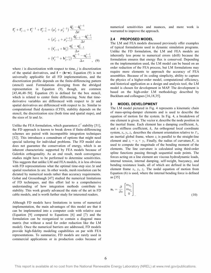
, (9) where i is discretization with respect to time, j is discretization of the spatial derivatives, and f = (h+w). Equation (9) is not universally applicable for all FD implementations, and the discretization profile depends on the finite-differencing pattern (stencil) used. Formulations diverging from the abridged representation in Equation (9), though, are common [45,46,48‒50]. Equation (9) is defined for the box stencil, which is related to center finite differencing. Note that time-derivative variables are differenced with respect to Δt and spatial derivatives are differenced with respect to Δs. Similar to computational fluid dynamics (CFD), stability depends on the stencil, the discretization size (both time and spatial steps), and the sizes of Δt and Δs. Unlike the FEA formulation, which guarantees L2 stability [51], the FD approach is known to break down if finite-differencing schemes are paired with incompatible integration techniques [52]. This introduces a conundrum of options that might need special tailoring for individual problems. The FD model also does not guarantee the conservation of energy, which is an inherent characteristic supported by FEA models because of Galerkin orthogonality. As an end result, mesh convergence studies might have to be performed to determine sensitivities. This suggests that unlike LM and FEA models, it is less obvious with FD representations what the optimal time-step size Δt and spatial resolution Δs are. In other words, mesh resolution can be dictated by numerical needs rather than accuracy requirements. Gobat and Grosenbaugh [47] studied the numerical limitations of FD techniques, and this effort led to a comprehensive understanding of how integration methods contribute to stability. This work greatly advanced the state of the art in FD cable models, and is worth further study for interested readers. Although FD models have limitations in terms of numerical implementation, the main advantages of this model are that it can be implemented into a computer code with relative ease (Equation [9] compared to Equations [6] and [7) and the formulation can be reorganized to contain a diagonal mass matrix (but without a need for order reduction like the LM model). Once the numerical barriers are addressed, FD models provide high-fidelity modeling capabilities on par with FEA representations. To summarize, FD models are rarely used in commercial applications or in production codes because of

numerical sensitivities and nuances, and more work is warranted to improve the approach.

2.4 PROPOSED MODEL The LM and FEA models discussed previously offer examples of typical formulations used in dynamic simulation programs. Unlike the FD formulation, the LM and FEA models are inherently less prone to numerical errors (drift) because the formulation ensures that energy flux is conserved. Depending on the implementation used, the LM model can be based on an order reduction of the FEA process, but LM formulations may require more elements to approach the accuracy of FEA assemblies. Because of its coding simplicity, ability to capture the physics of a higher-order model, computational efficiency, and historical application as a design and analysis tool, the LM model is chosen for development in MAP. The development is based on the high-order LM methodology described by Buckham and colleagues [16,18,35]. 3 MODEL DEVELOPMENT The LM model pictured in Fig. 4 represents a kinematic chain of mass-spring-damper elements and is used to describe the equation of motion for the system. In Fig. 4, a breakdown of one element is given. The vector ri describe the node position in the inertial frame. Each element has a damping coefficient, bi, and a stiffness coefficient, ki. An orthogonal local coordinate system, xi, yi, zi, describes the element orientation relative to F0, an inertial global frame, where zi is parallel to the straight-line element and zi = xi × yi. Finally, the radius of curvature, , is used to compute the magnitude of the bending moment of the elements. The line curvature is calculated using third-order spline functions passing through sequential node points. The forces acting on a line element are viscous hydrodynamic loads, internal tension, internal damping, self-weight, buoyancy, and bending resistance loads, all of which are defined in the local element frame xi, yi, zi. The nodal equation of motion from Equation (6) is used, where the internal bending force is defined as [35]

. (10)

7


FIGURE 4: DEFINITION OF ELEMENT AND NODE

COMPONENTS WITHIN THE LM MODEL. q(s) IS A CUBIC SPLINE FUNCTION INTERPOLATED THROUGH ALL THE

NODE POINTS.

3.1 LINE KINEMATICS Defining the line kinematics and system coordinate frame is the first step in obtaining the equation of motion. Alternative derivations can also be found in [16,18,27,28,31,35]. Let

(11) represent the transformation matrix relating the body-frame coordinates to a global inertial frame. As a result,

, (12) where Li + Δi is the stretched length of the ith element. From trigometric relations, the Euler angles θi and φi are given by

(13) and

(14) if cosθi > sinθi, and

(15)

otherwise. The inverse tangent calculation should capture angles across the full range of the unit circle (i.e., from 0–2π). From Equation (12), it is evident that the stretched line length is equivalent to the magnitude of the difference between ri and ri+1:

. (16) 3.2 INTERNAL FORCES Internal forces are derived from three sources: strain, damping, and bending resistance. Strain is proportional to the element stiffness, ki, which is the element axial stiffness EA/Li. Internal forces occur in the direction parallel to zi, so

(17) and

, (18) where Δi is readily known from Equation (16). Equation (17) is set to zero if Δi < 0, because cables cannot support compressive loads. Applying internal damping in structural members is a delicate issue [53], but it is generally accepted to be proportional to the relative velocity between nodes:

. (19) Deciding a coefficient for bi is a matter being debated within structural modeling circles, but a strong argument states that damping can be stiffness and mass proportional (i.e., Rayleigh damping) [11]. With certain integration schemes, though, structural damping is not recommended because this leads to conservative results [40]. This is especially true for most implicit integration techniques that include numerical dissipation. The effort of deriving the internal bending force was treated rigorously in [16,18,35]; readers are encouraged to refer to those texts for a detailed treatment of the bending stiffness formulation. As demonstrated by earlier works, the bending stiffness is given by the quantity

8


, (20)

where and equate the magnitude and axis (direction) at which the bending moment is applied in the local element frame. Equation (20) is expressed in an inertial reference frame consistent with Equation (6) once the Euler rotational sequence is performed. The spatial curvature parameter can be determined by [54]

, (21) where is the magnitude of the radius of curvature, is the

discrete form of q(s) to represent a three-dimensional cubic

spline expressed in a Frenet-Serret frame, and is the second

derivative of the spline function with respect to s. is a third-

order polynomial function evaluated for the ith element and is valid between the two nodes bounding an element:

. (22) It is essential for slopes of adjacent piece-wise elements to match, such that

. (23) An algorithm describing the process to obtain the piece-wise spline function can be found in [55]. The X,Y components of the curvature parameter are determined using

. (24) The slope of the cubic spline function passing through the nodes is the critical component to determine the bending force magnitude. When the spline function, , is a straight line, the

bending moment vanishes and Equation (20) is zero. As an

alternative, if a cable element can be represented by a straight-line spline function, Ci=Di=0 in Equation (22), and in Equation (21) is zero. 3.3 EXTERNAL FORCES External forces applied to the system arise from hydrodynamic loading, gravity, and seabed contact. To maximize code reuse and avoid duplicating actions performed in other FAST modules, hydrodynamic loads are calculated using a separate hydrodynamics module as exemplified in [56]. The hydrodynamic loads are based on the cable node motion and wave kinematics, which are used as input in a relative form of Morison’s equation to capture the element added-mass and quadratic drag forces. Buoyancy loads are also computed by the hydrodynamics module. The mapping of forces at discrete locations along the line occurs through the “mesh library,” which is a component defined in the FAST standard library [57]. Users only need to be concerned with providing the right inputs to the mesh library to obtain the desired outputs. More details on the mesh library are found in [64], but assuming the lumped hydrodynamic load, hx,y,z, is defined for the ith node, the force defined in vector form is

. (25) The terms resulting from gravity are found using

, (26) which is the net weight of the node in a vacuum. Seabed resistance forces are included through using an additional spring term. This spring is engaged when the Zi node position drops below a certain threshold. The formulation for this quantity resembles Equation (17), but requires Equation (18) to be rewritten to include this additional force. Some formulations include a two-parameter spring model with damping to relax the recoiling effect caused by a sudden onset of the contact force [14,48]. 3.4 CABLE STATICS Cable statics are an important preliminary step in running a dynamics simulation, but numerical limitations drive this delicate matter. Because the objective of a dynamic mooring line model is to address a dynamics problem, the statics problem is largely viewed as an afterthought. The performance of the dynamic model, however, is strongly dependent on the quality of the initial starting point of the nodes and stretched element lengths. A statics solution is achieved by removing all time-dependent variables in Equation (6), then solving the resulting nonlinear

9


equations. Minimizing these functions is an immensely difficult task because the Jacobian matrix used by the nonlinear root-finding algorithm is poorly conditioned [44]. Several approaches to solving the statics problem exist, and the chosen path is a matter of preference. The simple approach is dynamic relaxation [58,59], which involves executing a dynamics simulation with large damping values until transients dissipate. Another approach implements an artificial force term into Equation (6) that is initially set equal to the (unbalanced) node forces [19,60,61]

, (27) where the j subscript is the solve step. For the first solve step,

, (28) βj ranges from {1,0}, where βi = 1 at the first solve, and βj = 0 at convergence. A third approach uses a shooting algorithm, which involves a rewrite of the equations being solved by converting Equation (6) from an initial value problem to a boundary condition problem [44,62,63]. The approach to be implemented in MAP will be selected from one of these methods.

4 FAST FRAMEWORK AMALGAMATION The FAST modularization framework can be considered to be an application program interface that defines the guidelines and standard practices for modules being integrated into the latest version of the FAST wind turbine CAE tool [1,57]. This framework compartmentalizes different components modeled in the wind turbine to separate the physics of the system. Although for most modules, communication with other modules is essential (such as hydrodynamic force mapping on a structural model [56]), the information-passing corridor is managed by the

FAST glue code. In this regard, module developers are responsible for defining the quantities exchanged between modules and the information passed to and from FAST. This leads to extensible modules that can be separated away from the core glue code, allowing modules to conduct independent studies without redefining the source code. To draw parallels between the LM model and the FAST framework, the single-point mooring in Fig. 3 is used to define a mooring anchored to the seabed at node N+1 and attached to a floating wind turbine at node 1. Figure 5 demonstrates the flow of information between FAST and the proposed LM component of the MAP module. The passage of information and program flow illustrated falls under the auspice of the FAST “loose-coupling” definition. Under the loose-coupling definition, each individual module is responsible for executing the solve routines and integration of differential equations (when necessary) for that module. The particular definition of each data structure is interpreted by the FAST glue code to describe the action taken on that variable. 4.1 DATA STRUCTURES Data structures are used to define the interaction of variables between the FAST glue code and modules. For example, parameters p are constant, time-invariant values throughout the simulation, such as sea density, gravitational constant, or the anchor position of a line element. Likewise, continuous states, x(t), are those with which a differential equation is associated [57]

. (29) Constraint states z are variables iterated by a root-finding algorithm to find the minimum of a function

FIGURE 5: INPUTS, OUTPUTS, AND INTERNAL STATES FOR THE LM MODULE IN MAP. THIS FLOWCHART IS DEFINED FOR LOOSE COUPLING [1,56,57].

10


, (30)

with a requirement that

. (31) Otherwise, the matrix in Equation (31) is rank deficient and a bounded inverse does not exist around a solution. Equation (31) is defined as the Jacobian matrix determinant, where the Jacobian matrix is used to find the roots of Equation (30). It becomes evident from Equations (29) and (30) that FAST is formulated as a multibody dynamics system and the solution is structured as a DAE [42]. The formulation, though, reduces to a conventional ODE when constraints z are not present. In the context of a dynamic cable model for FAST, the inputs to MAP would be the position and velocity of the node attaching to the floating platform and hydrodynamic loads on all nodes:

. (32) The values in Equation (32) are transferred from the glue code using a mesh, because the node position and velocity are related to the platform global motion as computed by FAST. Outputs from MAP consist of the force and moment at the node attaching to the platform, and the position and velocity of all intermediate nodes between the fairlead and anchor. The intermediate nodes are mapped as meshes so kinematic information can be received by an external hydrodynamics module to calculate viscous loads. As a result,

, (33) where the moments mbx

1 and mby

1 at the cable root are

calculated using the procedure in [35]. The output vector is information passed back to the FAST glue code to advance to the next time-step sequence. In this application, the constraint variable, z, consists of the coefficients’ cubic polynomial function, , in Equation (22). As a result, the constraints are

. (34) The continuous state consists of nodes whose position and velocity are obtained by way of numerical integration. They are defined as the nodes lying between the anchor point and fairlead:

. (35) The node attaching to the floating vessel at i=1 has prescribed motion supplied by the FAST glue code, and it does not have an associated differential equation. Likewise, the anchor node is fixed, so it is encapsulated within p. The remaining variables, such as , θi and φi , are preserved in a database named “other states.” Storage of these variables in the other states derived type is allowable because they are explicitly derived from x, z, p, or u. 4.2 EQUATIONS In this application of the LM model, two sets of equations are necessary to complete the FAST definitions. The first, the continuous equations, are those that can be differentiated with time. This was previously defined in Equation (6), rewritten as the following ODE:

. (36) The second state equations, the constraint equations, are those iterating on the constraint variables, z(t), to minimize a function. In this case, the functions minimized are those providing the solution to the cubic spline interpolation function in Equation (22). An example algorithm is given in [55]. 5 SUMMARY This paper surveys the various dynamic modeling line theories that are currently used in offshore modeling applications. Advantages of each model are considered, and although each model has merit, the LM model is selected for incorporation in MAP. The LM model is selected for the following reasons: Computational performance is optimized for diverse

applications: A diagonal mass matrix may omit acceleration

coupling terms, but limitations can be rectified by increasing the mesh resolution.

11


• Sensitivities of the numerical approaches are well studied. • Incorporation of bending stiffness is available as a user

option: − Over the past two decades, the abilities of LM models

have improved significantly to the extent that high-order bending stiffness models have been included.

− Bending can be disabled at run time. When bending stiffness is disabled, ni = 0 in Equation (6).

Equations describing the LM model are reconstructed in the FAST framework context. Although this paper explores the framework from a loose-coupling standpoint, this model can be expanded to include essentials for tight coupling. As a land-based and floating wind turbine modeling tool, FAST is responsible for combining several physics to aid in the simulation of these devices. To assist in the integration of various physics, the modularization framework has been developed to help encapsulate data, encourage code reuse, and enable state linearization (e.g., for eigen analysis) and tight-coupling dynamic analysis. This paper explains a new dynamic mooring line module in the context of this new framework. MAP is a module developed for FAST that is currently capable of quasi-static modeling. By adding a dynamic mooring line representation, MAP will enable coupled analysis in FAST. Future work will involve implementation, verification, and validation of this LM model within MAP and application of the coupled code to the analysis of promising floating offshore wind concepts. REFERENCES [1] Jonkman, J., and Buhl, M., 2005, “FAST User’s Guide,”

NREL/EL-500-38230, NREL, Golden, CO. [2] Jonkman, J., 2013, “The New Modularization Framework

for the FAST Wind Turbine CAE Tool,” 51st AIAA Aerospace Meeting, Dallas, TX, January 7–10.

[3] Masciola, M., Jonkman, J., and Robertson, A., 2013, “Implementation of a Multisegmented, Quasi-Static Cable Model,” 23rd International Offshore and Polar Engineering (ISOPE) Conference, Anchorage, AK, June 30–July 5.

[4] Peyrot, A. H., and Goulois, A. M., 1979, “Analysis of Cable Structures,” J. Computer & Structures, 10, pp. 805–813.

[5] Mekha, B., Johnson, C., and Roesset, J., 1996, “Implications of Tendon Modeling on Nonlinear Response of TLP,” J. Structural Eng., 122(2), 142–149.

[6] Adrezin, R., Bar-Avi, P., and Benaroya, H., 1996, “Dynamic Response of Compliant Offshore Structures – Review,” J. Aerospace Eng., 9(4), 114–131.

[7] Irvine, M., 1993, Cable Structures, Dover Publications, Mineola, NY.

[8] Chai, Y., Varyani, K., and Barltrop, N., 2002, “Semianalytical Quasi-Static Formulation for Three-Dimensional Partially Grounded Mooring System Problems,” Ocean Eng., 29, pp. 627–649.

[9] Griffin, O. M., and Rosenthal, F., 1989, “The Dynamic Of Slack Marine Cables,” J. Offshore Mech. Arct. Eng., 11(4), pp. 298–302.

[10] Starossek, U., 1994, “Cable Dynamics – a Review,” J. Structural Eng. Int., 4, pp. 171–176.

[11] Inman, D., 2007, Engineering Vibrations, Prentice Hall, Upper Saddle River, NJ.

[12] Masciola, M., Nahon, M., and Driscoll, F., 2012, “Preliminary Assessment of the Importance of Platform-Tendon Coupling in a Tension Leg Platform,” J. Offshore Mech. Arct. Eng., 135(3).

[13] Masciola, M., Jonkman, J., Robertson, A., Coulling, A., and Goupee, A., 2013, “Assessment of the Importance of Mooring Dynamics on the Global Response of the DeepCwind Floating Semisubmersible Offshore Wind Turbine,” 23rd International Offshore and Polar Engineering (ISOPE) Conference, Anchorage, AK, June 30–July 5.

[14] Gatti-Bono, C., and Perkins, N. C., 2004, “Numerical Simulations of Cable/Seabed Interactions,” J. Int. Soc. Offshore and Polar Eng., 14(2).

[15] Nicoll, R. A., 2004, “Dynamic Simulation of Marine Risers with Vortex Induced Vibrations,” Master’s Thesis, University of Victoria, British Columbia, Canada.

[16] Buckham, B., Driscoll, F. R., and Nahon, M., 2004, “Development of a Finite Element Cable Model for Use in Low-Tension Dynamics Simulation,” J. Applied Mech., 71(4), pp. 476–485.

[17] Dalane, J. I., 1997, “Fatigue Reliability – Measured Response of the Heidrun TLP Tethers,” Marine Structures, 10(10), pp. 611–628.

[18] Buckham, B., Nahon, M., Seto, M., Zhao, X., and Lambert, C., 2003, “Dynamic of a Towed Underwater Vehicle System: Part 1: Model Development,” Ocean Eng., 30(4), pp. 453–470.

[19] Powell, G., and Simons, J., 1981, “Improved Iteration Strategy for Nonlinear Structures,” J. Numerical Methods in Eng., 17, pp. 1455–1467.

[20] Walton, T. S., and Polacheck, W., 1960, “Calculation of Transient Motion of Submerged Cables,” Mathematics of Computation, 14(69), pp. 27–46.

[21] Turner, M. J., Clough, R. W., Martin, H. C., and Topp, L. J., 1956, “Stiffness and Deflection Analysis of Complex Structures,” J. Aeronautical Sciences, 23(9), pp. 805–854.

[22] Merchant, H. C., and Kelf, M. A., 1973, “Non-Linear Analysis of Submerged Buoy Systems,” Proc. MTS/IEEE Oceans, 1, pp. 390–395.

[23] Ketchman, J. J., and Lou, Y. K., 1975, “Application of the Finite Element Method to Towed Cable Dynamics,” Proc. MTS/IEEE Oceans, 1, 98–107.

12


[24] Nordgren, R. P., 1974, “On the Computation of the Motion of Elastic Rods,” J. Applied Mechanics, 4(2), pp. 777–780.

[25] Garret, D. L., 1982, “Dynamic Analysis of Slender Rods,” J. Energy Resource Technology, 104, pp. 302–306.

[26] Zienkiewicz, O. C., and Taylor, R. L., 1977, The Finite Element Method, Vol. 3, McGraw-Hill, London, UK.

[27] Lambert, C., Nahon, M., and Chalmers, D., 2007, “Implementation of an Aerial Positioning System with Cable Control,” IEEE/ASME Transactions on Mechatronics, 12(1), pp. 32–40.

[28] Nahon, M., 1999, “Dynamics and Control of a Novel Radio Telescope Antenna,” AIAA Modeling and Simulation Technologies Conference and Exhibit, pp. 214–222.

[29] Huang, S., 1994, “Dynamic Analysis of Three-Dimensional Marine Cables,” J. Waterway, Port Coastal, and Ocean Eng., 21(6), pp. 587–605.

[30] Williams, P., Trivaila, P., 2007, “Dynamics of Circularly Towered Cable Systems, Part 1: Optimal Configurations an their Stability,” J. Guidance, Control and Dynamics, 30(2), pp. 753–765.

[31] Driscoll, F., Lueck, R., and Nahon, M., 2000, “Development and Validation of a Lumped-Mass Dynamics Model of a Deepsea ROV System,” Applied Ocean Research, 22(3), pp. 169–182.

[32] Golub, G., and Van Loan, C. F., 1996, Matrix Computations, 3rd Ed., Johns Hopkins, Baltimore, MD.

[33] Ran, Z., 2000, “Coupled Dynamic Analysis of Floating Structures in Waves and Currents,” Ph.D. Thesis, Texas A&M University, College Station, TX.

[34] Rupe, R. C., and Thresher, R. W., 1975, “The Anchor-Last Deployment Problem for Inextensible Mooring Lines,” Transactions of the ASME, (74-WA), pp. 1046–1052.

[35] Buckham, B. J., 2003, “Dynamics Modeling of Low-Tension Tethers for Submerged Remotely Operated Vehicles,” Ph.D. Thesis, University of Victoria, British Columbia, Canada.

[36] Kennedy, R. M., 1981, “Crosstrack Dynamics of a Long Cable Towed in the Ocean,” IEEE OCEANS’81, Boston, MA, September 16–18, pp. 966–970.

[37] Lo, A., and Leonard, J. W., 1982, “Dynamic Analysis of Underwater Cables,” J. Eng. Mechanics Division, 108(4), pp. 605–621.

[38] Leonard, J. W., and Nath, J. H., 1981, “Comparison of Finite Element and Lumped Parameter Method for Oceanic Cables,” Eng. Structures, 3(3), pp. 153–167.

[39] Wang, P. H., Fung, R. F., and Lee, M. J., 1998, “Finite Element Analysis of a Three-Dimensional Underwater Cable with Time-Dependent Length,” J. Sound and Vibration, 209(2), pp. 223–249.

[40] Chung, J., and Hulbert, G. M., 1993, “A Time Integration Algorithm for Structural Dynamic with Improved Numerical Dissipation: the Generalize-α Method,” J. App. Mech., 60, pp. 371–375.

[41] Garrett, D. L., 2005, “Coupled Analysis of Floating Production Systems,” Ocean Eng., 32, pp. 802–816.

[42] Asher, U. M., and Petzold, L. R., 1998, “Computer Methods for Ordinary-Differential Equations and Differential-Algebraic Equations,” Society for Industrial and Applied Mathematics (SIAM), Philadelphia, PA.

[43] Kaczmarczyk, S., and Ostachowicz, W., 2003, “Transient Vibration Phenomena in Deep Mine Hoisting Cables: Part 1: Mathematical Model,” J. Sound and Vibration, 363(2), pp. 219–244.

[44] Masciola, M., Nahon, M., and Driscoll, F., 2012, “Static Analysis of the Lumped Mass Cable Model Using a Shooting Algorithm,” J. Waterway, Port, Coastal, Ocean Eng., 138(2), pp. 164–171.

[45] Chiou, R., 1989, “Nonlinear Hydrodynamic Response of Curved Singly Connected Cables,” Ph.D. Thesis, Oregon State University, Corvallis, OR.

[46] Gobat, J., 2000, “The Dynamics of Geometrically Compliant Mooring Systems,” Ph.D. Thesis, Woods Hole Oceanographic Institute and Massachusetts Institute of Technology, Woods Hole, MA.

[47] Gobat, J., and Grosenbaugh, M., 2006, “Time-Domain Numerical Simulation of Ocean Cable Structures,” Ocean Eng., 33(10), pp. 1373–1400.

[48] Sachin, G., and Perkins, N. C., 2007, “Modeling of Cables with High and Low Tension Zones Using a Hybrid Rod-Catenary Formulation, arXiv preprint Physics/0702224.

[49] Mehrabi, A., and Tabatabai, H., 1998, “Unified Finite Difference Formulation for Free Vibration of Cables,” J. Struct. Eng., 124(11), pp. 1313–1322.

[50] Ablow, C. M., and Schechter, S., 1983, “Numerical Simulation of Undersea Cable Dynamics,” Ocean Eng., 10, pp. 443–457.

[51] Liu, Y., Shu, C. W., Tadmor, E., and Zhang, M., 2002, “L2 Stability Analysis of the Discontinuous Galerkin Method and a Comparison between the Central and Regular Discontinuous Galerkin Methods,” Georgia Institute of Technology, Atlanta School of Mathematics, Atlanta, GA.

[52] Hughes, T. J. R., 1977, “Unconditionally Stable Algorithms for Nonlinear Heat Conduction,” Comp. Methods in App. Mech. and Eng., 10, pp. 135–139.

[53] Hall, J. F., 2006, “Problems Encountered from the Use (or Misuse) of Rayleigh Damping,” Earthquake Eng. & Struct. Dynamics, 35(5), pp. 525–545.

[54] O’Neill, B., 1966, Elementary Differential Geometry, Academic Press, New York, NY.

[55] Flannery, B. P., Press, W. H., Teukolosky, S. A., and Vetterline, W., 1992, Numerical Recipes in C, Press Syndicate of University of Cambridge, New York, NY.

[56] Song, H., Damiani, R., Robertson, A., and Jonkman, J., 2013, “A New Structural-Dynamics Module for Offshore Multimember Substructures within the Wind Turbine Computer-Aided Engineering Tool FAST,” 23rd International Offshore and Polar Engineering (ISOPE) Conference, Anchorage, AK, June 30–July 5.

13


[57] Jonkman, J., 2013, “The New Modularization Framework for the FAST Wind Turbine CAE Tool,” 51st AIAA Aerospace Sciences Meeting, Dallas, TX, January 7–10.

[58] Webster, R. L., 1980, “On the Static Analysis of Structures with Strong Geometric Nonlinearity,” Computers & Structures, 11(1), pp. 137–145.

[59] Wu, S., 1995, “Adaptive Dynamic Relaxation Technique for Static Analysis of Catenary Mooring,” Marine Structures, 8(5), pp. 585–599.

[60] Zueck, R., 1995, “Stable Numerical Solver for Cable Structures,” Int. Symposium on Cable Dynamics, Liege, Belgium.

[61] Powell, G., and Simons, J., 1981, “Improved Iteration Strategy for Nonlinear Structures,” J. Numerical Methods in Eng., 17(10), pp. 1455–1467.

[62] De Zoysa, A. P. K., 1978, “Steady-State Analysis of Undersea Cable,” Ocean Eng., 5(3), pp. 209–223.

[63] Friswell, M., 1995, “Steady-State Analysis of Underwater Cables,” J. Waterway, Port, Coastal, Ocean Eng., 121(2), pp. 98–104.

[64] Sprague, M. A., Jonkman, J. M., and Jonkman, B. J., 2014, “FAST Modular Wind Turbine CASE Tool: Nonmatching Spatial and Temporal Meshes,” AIAA Science and Technology Forum (SciTech 2014), Reston VA, January 13–17.

extending the capabilities of the mooring analysis … of dynamic mooring ... apparatus, product, or...

Documents