extending the data warehouse for service provisioning data … · · 2008-03-20extending the data...

Data & Knowledge Engineering 59 (2006) 700–724

www.elsevier.com/locate/datak

Extending the data warehouse for service provisioning data

Yannis Kotidis *

AT&T Labs-Research, 180 Park Ave., Florham Park, NJ 07932, United States

Received 1 December 2004; received in revised form 14 November 2005; accepted 15 November 2005Available online 15 December 2005

Abstract

The last few years, there has been an extensive body of literature in data warehousing applications that primarily focuseson basket-type (transactional) data, common in retail industries. In this paper we focus on service provisioning data, that isdata that is recorded internally in an organization for provisioning certain business related tasks. Coupling the recordeddata with the underlying process and business-practice(s) that generate them is crucial for end-to-end analysis. Our frame-work is based on a graph description of the process (called a sketch) that is generating this data. Using this sketch, we for-malize a new class of aggregate queries that consolidate data from a part of the process, based on a user defined pathexpression. We then show how to build a compact, non-redundant collection of summary (aggregate) tables and indicesfor this new type of queries. We first explore how to select a minimum set of views to answer queries with path-expressionsover the given sketch. For queries that also include aggregation, we define two partial orders among the views. The first isused to pick the minimum set of aggregate views to answer any query with no false dismissals, while the second describes anaugmented set that allows fewer false positives. Computing a non-materialized aggregate is done through appropriaterewriting of the user query. We describe two indexing schemes that use phantom (non-materialized) aggregate values to expe-dite query processing. Experimental results show these schemes to perform well on synthetic and real datasets.� 2005 Elsevier B.V. All rights reserved.

Keywords: Data warehouse; Workflow; Materialized views

1. Introduction

The astonishing success of information technology has resulted in an explosive growth in the amount ofdata that is being recorded in daily basis on various domains. This abundance of data has in-turn driventhe data warehousing sector into a major segment of the information technology market and, subsequently,has attracted a lot of interest from the academic community. The data warehouse is an integrated informa-tional store that provides stable, point-in-time data for decision support applications. Data-rich industries,like retail and financial services, have been the most typical users of data warehousing technology for the obvi-ous reason that they have large quantities of good quality internal and external data available, to which theyneed to add value.

0169-023X/$ - see front matter � 2005 Elsevier B.V. All rights reserved.

doi:10.1016/j.datak.2005.11.003

* Tel.: +1 9733608347.E-mail addresses: [email protected], [email protected]

mailto:[email protected]

mailto:[email protected]

Y. Kotidis / Data & Knowledge Engineering 59 (2006) 700–724 701

Often data is recorded internally in an organization for provisioning certain business related tasks. Duringthe last few decades there has been an increasing trend to computerize every possible business process andeliminate manual hand-offs. Workflow management and Customer Relationship Management (CRM) soft-ware are being used to help manage customer relationships in an efficient and organized manner. For example,in the telecom sector, accepting a new customer for long distance service involves several steps from entry andverification of personal data to third party verification (a process in which a designated third party confirmsthe customer’s intention to change service), and finally placing a new entry in the company’s billing database.A process known as revenue assurance verifies the beginning-to-end completeness, accuracy, and integrity ofthe capture, recording, billing, and reporting of all revenue-producing events from customer order entrythrough collection.

The type of data generated from these processes does not conform to the basket paradigm, regularly used indata warehousing. Informally, a service provisioning database contains a large collection of customer records.Each record describes a sequence of events that captures the interaction between a customer’s order and var-ious components of the organization. Presumably, there is a well defined workflow that describes the flow ofevents for incorporating a customer’s order [43]. Each customer record is an instance of some part of thisworkflow process annotated with timing information and other business related attributes. Each order is thentreated as an ‘‘entity’’, which flows through the service’s workflow. Network traffic is another example inwhich the recorded data conforms to an underlying structure: the network topology. Any end-to-end commu-nication of network elements uses a collection of network paths directed by the routing protocols and thephysical interconnect among them.

When trying to apply conventional data warehousing techniques for a service provisioning database, we arefaced with the problem of mapping the recorded data into a relational schema in a way that allows complexanalytical queries over the recorded information with respect to the structural properties of the process thatgenerates these records. In our framework, the user expresses his intention to analyze the data at a particularresolution for some portion of the process by providing what we call a sketch of the process. The sketch is agraph representation of the underlying process, containing nodes representing ‘‘states’’ and edges representing‘‘transitions’’. Given a sketch, we explore how to build a compact, non-redundant collection of summarytables and indices to facilitate flexible decision support analysis.

As we will demonstrate, conventional relational implementations are incapable of providing flexible ana-lysis of the recorded data with respect to a given sketch [16]. In the basket-data paradigm a multi-dimensionalapproach is used, in which data, representing transactions, is projected and aggregated using a set of dimen-sions (like products and customers). In a service provisioning database the structural properties of the sketchare the dimensions of interest. In this paper we introduce pair-wise aggregate queries as a means to describethe scope of an interesting aggregation. Such a query consists of a path expression over the graph (sketch) thatcollects relevant recorded information from parts of the underlying process and a user defined aggregate func-tion F that consolidates this data. We first formally define pair-wise aggregate queries and then show how toexpress more complex expressions and evaluate them as a series of pair-wise queries. In addition, we exploreoperations that allow us to zoom in and out of certain states of the process, or exclude parts we are not inter-esting in. As will be explained these operations are naturally mapped into pair-wise queries that consolidatethe underlying records.

For large datasets, evaluating pair-wise aggregate queries on the fly can be prohibitively expensive. Oftenthere is no efficient way to simultaneously evaluate path and aggregate expressions over the data. Materializedviews can be used to speed up query processing and also shield the user from the details of mapping a complexaggregate expression to the underlying relational schema. We first show how to optimize execution of querieswith path expressions using a non-redundant collection of views materialized as bitmapped indexes [10,42,50].For queries that also contain aggregations we propose the use of pair-wise aggregate views that contain pre-computed results of pair-wise queries and discuss different materialization policies. These views can be used toanswer arbitrary pair-wise aggregate queries without imposing any false negatives (i.e. omit records thatshould have been in the answer) and with provably less cost than a regular index scan. We then show howto rewrite queries to use these views based on a partial order that we define among them. This rewriting worksefficiently using an indexing scheme that partitions the records of a view on non-materialized phantom aggre-

gates, in a way that allows efficient evaluation of subsequent queries against these aggregates.

702 Y. Kotidis / Data & Knowledge Engineering 59 (2006) 700–724

1.1. Map

The rest of the paper is organized as follows: Section 2 motivates the problem from two practical applica-tions. Section 3 discusses related work. In Section 4 we introduce our framework, define pair-wise queries andmaterialized pair-wise views and discuss the shortcomings of various relational models for the service provi-sioning data. In Sections 5 and 6 we show how to choose from, index and query these aggregate views foranswering user queries. Finally Section 7 contains the experiments and in Section 8 we draw the conclusions.

2. Motivation

We here present two examples of service provisioning that will help us better motivate the discussion.

2.1. Telephone service provisioning

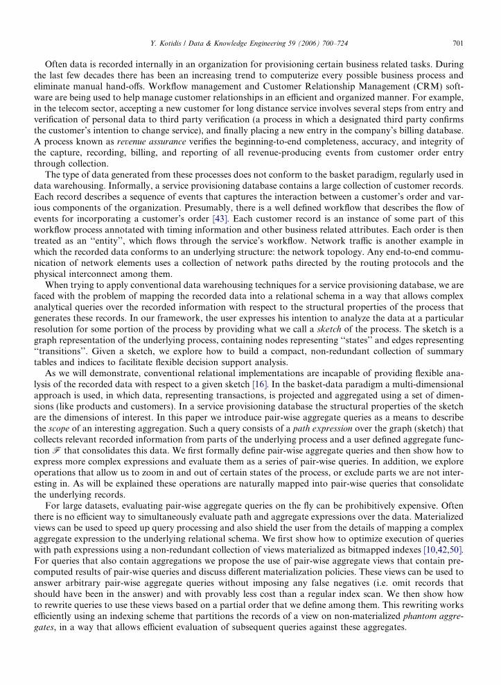
Telephone service provisioning includes several steps, starting with the reception of customer’s order andending with the establishment (or modification) of service. The workflows related to this process are typicallyvery complicated because orders require processing by many departments. Fig. 1 provides a simplified highlevel view of this workflow for long distance orders. There are five major states modeled in this example. Cre-

ate involves all actions related to the reception and creation of a new order. TPV stands for third-party ver-ification and LEC stands for Local Exchange Carrier. The latter state includes all communications with theLEC to establish the caller as a new customer. State Billing involves all actions related to creation or modi-fication of a customer’s billing record. Finally, state Complete denotes the successful completion of the wholeprocess. A customer’s order is modeled as an entity that flows through this process. States TPV and LEC areonly used for orders that involve creation of a new long distance service. Orders of customers that call to mod-ify their plans (e.g. sign to a new promotion) skip these states. Each of the five main states can be expandedand modeled in more details. Depending on the application, we might want to ‘‘drill-down’’ on a state andanalyze the flow of records at a finer granularity.

The user expresses his intention to analyze the data at a particular resolution for some portion of this pro-cess by providing what we call a sketch. A sketch is a directed acyclic graph (DAG) describing states and tran-sitions that he is interested in (later on we extend our discussion for sketches with cycles). For example if theuser is interested in the five depicted states of the workflow of Fig. 1, the sketch is simply a DAG represen-tation of the process in which each state is mapped to a node and each transition is mapped to an edge. Inthis example the process at this particular level happens to be acyclic too but this is not required in general.

A sketch is an abstraction of the whole process and is used to filter those events that flow through the spec-ified nodes and edges of the DAG. For example if there were a Failed state in the process that is not included inthe sketch then the analysis will only target records of orders that have successfully completed. Analysis will bebased on data attributes collected by the recording mechanisms as well as the structural properties of the givensketch. Examples of such queries include:

1. Retrieve all orders that passed through states TPV and LEC (e.g. new long distance customers).2. Find all orders for which an intermediate transition from state Create to state Complete took more than 8 h,

while the order was completed in less than a day (e.g. trace ‘‘hidden delays’’).3. Find all orders that were modified (possibly due to initial data entry errors) more than once between states

TPV and Billing.

Create

TPV LEC

Billing Complete

Fig. 1. Telephone service provisioning example.

SS H1 H2 H3 TT

H0

Fig. 2. Delivery service provisioning example.


Query (1) is an example of a path-query, discussed in Section 5. Query (2) inquires timing informationrecorded as the order flows through the process. This is critical for most service ordering systems as user sat-isfaction is primarily based on timely processing of his orders [6,17]. Surprisingly, the area of handling time-related issues and detecting potential problems has not received adequate attention in the workflow literature[17]. For query (3) we exploit a version attribute attached to each record that counts all modifications to theorder.

2.2. Delivery service provisioning

Fig. 2 depicts a number of ‘‘hubs’’ Hi that are used to interconnect two sites S and T. Examples of such ascenario can be found in different domains. In a network service provisioning system, S and T can be two sub-networks and hubs Hi will be the network elements (e.g. routers) that provide the interconnect among thesetwo networks. In a packet delivery service (like FedEx) the picture of Fig. 2 may describe the network of com-pany’s locations and the connectivity among them. Connecting paths may have different capacities, band-width, latencies etc. Some connections are bi-directional while others not, as shown in the figure. Assumingthat we want to provision delivery of services from site S to site T, our sketch is obtained by making allbi-directional edges in the figure be pointing from left to right. Given this sketch, the queries that we are inter-ested in include:

4. Find all flows from S to T that utilized hub H0.5. Find all flows from S to T that stopped at least at 3 hubs.6. Find all flows from H1 to H3 for which each transition required at least 1 day.

Query (4) is a simplified path-query on a single node. In query (5) we ‘‘aggregate’’ multiple paths from S toT by counting the number of intermediate hubs in a flow from S to T. An equivalent, but more cumbersome,way to state the query is to ask for all flows of the form S! H1! H2! H3! T, S! H0! H1!H2! H3! T or S! H0! H1! H3! T. Finally query (6) requests a specific path from the sketch alongwith additional timing constraints.

3. Related work

Within the past decade we have witnessed renewed excitement in decision support tools and applications.Advances in information technology and globalization of businesses created the right combination of ‘‘sup-ply’’ and ‘‘demand’’ to fuel the data warehousing field.

The primal goal of a data warehouse is to provide an integrated data store for the execution of complexanalytical queries. Such queries often involve aggregation. Because of the size of the data at-hand and theplethora of choices for ad hoc grouping and aggregation, data warehouses rely on pre-computation and exten-sive indexing of the data. Bitmapped indexes and their variations [41,10,42,50] have found their way into mostindustrial solutions. Another form of pre-computation is the use of materialized views containing frequentlyasked aggregates. Engineering questions, such as how many and which views to materialize under a space and/or update time constraint and an expected query workload have led to several view selection algorithms[28,47,48,27,4] as well as alternative dynamic organizations [34,45,46]. In this paper, we too rely on pre-com-putation for speeding up aggregate queries that arise in the process of analyzing service provisioning data. Ourdefinition of pair-wise queries has been motivated from related literature on recursive queries (e.g.


[35,31,44,49]). As will be explained, we use the structural properties of the underlying process that generatesthe data to define a partial order among the views. Our primary focus is on selecting the minimum number ofviews that can answer any query of interest without false dismissals. If additional resources are available, usingthe partial order we define among the views, one can easily modify the algorithms of e.g. [28] for selectingadditional views in the materialized set. Implementation of the aggregate views we discuss in this paper canbe done using bitmapped indexes and other standard relational tools like B-trees. We further exploit thedependencies among the views (that have been discovered from analyzing the process) to extend traditionalindexing schemes and achieve even better query performance.

Dimensional modeling is a specialization of the traditional ER modeling [12,40]. It distinguishes facts (likecredit-card transactions), from dimensions that provide a context for the facts (like time, product, location).Most common examples of dimensional modeling include the stars schema, the snowflake schema and theirextensions like the federated star schemas [33,11]. In the service provision example, the underlying processprovides the context within which data is modeled and analyzed. In this paper, we assume that the underlyingprocess is given. When the process is unknown, one can infer it using mining techniques such as the onesdescribed in [1,14].

Workflow management systems are extensively used for process simulation, in order to identify bottlenecksand analyze execution durations of business tasks [17,38,30]. They are also used in office automation forassignment of tasks and execution monitoring (triggering alarms when deadlines are missed, exemptionhandling etc.) [32]. In the database community there has been extensive work on extending transactions forworkflow applications [13,39,9,5,21,7,3]. In this paper we focus on modeling and organizing the data forpost-processing and analysis. Our work aims on utilizing existing data warehousing techniques for the process-ing and analysis of data generated from real business processes. This is an area that has received little attentionin the literature. Grigori et al. in [26] discuss a set of Business Process Intelligence tools for cleaning and aggre-gating workflow logs into a warehouse for analysis, prediction and optimization of business processes. In [18]the authors make a case for using data On-Line Analytical Processing (OLAP) tools in analyzing workflowlogs and present a generic data warehouse design. In [8] the authors identify some major challenges in design-ing data warehouses for managing workflow data such as the presence of multiple related facts that lead tocomplicated schemas, the complexity of aggregations required due to this fact and the volatility of workflowmodels that may require frequent substantial changes in the warehouse design. The authors of [36] follow anobject-oriented approach driven by use case and object models for modeling business requirements for thedata warehouse.

4. A framework for service provisioning data

4.1. Data model

We first provide a formal definition of a sketch. Given a process that is being provisioned, a sketch is adirected acyclic graph G(V,E) with the following properties: each node v in V corresponds to a particular stateof the process (seen at the desirable resolution). An edge e = (v1,v2) represents a valid transition between cor-responding states v1 and v2 in the process that we are observing. There is a set S 2 V of starting nodes in thesketch i.e. nodes that have no incoming edges in G(V,E). Similarly all nodes with no outgoing edges form a setof terminal nodes T. In Section 5.3 we extend the definition to graphs that include cycles.

A record r is called relevant to a sketch G(V,E) if it describes a transition from some starting node s 2 S to aterminal node t 2 T through nodes of V � S � T using edges in E. For this model we assume that informationis being recorded at every edge traversed in r and stored in attributes called measures. For simplicity in thenotation we will only refer to examples with a single numeric measure denoted as x. In that case, a recordr is an ordered set of pairs:

r ¼ fðe1; x1Þ; . . . ; ðekr ; xkrÞg ð1Þ
R denotes the whole collection of records that are relevant to the sketch. Sometimes, specific nodes may havemeasure data recorded too. This is useful in order to trace intra-node processing. In these cases, we replacesuch a node v with a linked pair v1, v2. Edge (v1,v2) is then used to store the intra-node measure.

A B C E

F

D

Fig. 3. Simple sketch.

Table 1Examples of valid records for the sketch of Fig. 3

Original representation Dual representation

r1 = {(e(A,B), 5), (e(B,C), 7), (e(C,D), 8), (e(D,E), 2)} rd1 ¼ fðvA; 5Þ; ðvB; 7Þ; ðvC ; 8Þ; ðvD; 2Þ; ðvE ;aÞg

r2 = {(e(A,B), 6), (e(B,D), 4), (e(D,E), 3)} rd2 ¼ fðvA; 6Þ; ðvB; 8Þ; ðvD; 3Þ; ðvE;aÞg

r3 = {(e(A,B), 4), (e(B,F), 1)} rd3 ¼ fðvA; 4Þ; ðvB; 1Þ; ðvF ;aÞg


A dual representation of a record, denoted as rd is derived by using state information 1:

1 a dbe om

rd ¼ fðve11 ; x1Þ; ðve2

1 ; x2Þ; . . . ; ðvekr1 ; xkrÞ; ðv

ekr2 ;aÞg ð2Þ

As a running example we will be using the sketch of Fig. 3. Node A is a starting node and nodes F, E

are terminal nodes. Table 1 shows examples of relevant records for that sketch in their original and dualrepresentation.

When information is only recorded at the nodes, we use notation (1) on the dual graph of the sketch (e.g. byswitching nodes and edges).

4.2. Pair-wise queries

In OLAP, a multi-dimensional approach to analysis is used to align the data content with the analyst’smental model. In the basket-data paradigm such dimensions are the products and customers involved in atransaction [24]. The measures are then projected and evaluated over the selected dimensions. In a service pro-visioning database the structural properties of the sketch are the dimensions of interest.

In order to analyze the data we need to specify parts of the sketch as the scope of our analysis and thencompute interesting aggregates on the relevant measures. Since G is acyclic, any two distinct nodes u and v

for which there is a path u! v = (u = v1,v2, . . . ,vk = v) from u to v in G define a selection filter over the storedrecords.

Definition 4.1. A pair-wise selection filter Su!vðRÞ returns all records that contain a transition from u to v.For each qualifying record r ¼ fðe1; x1Þ; . . . ; ðekr ; xkrÞg there exist i, j such that 1 6 i 6 j 6 kr and ei = (u, ?),ej = (?, v), where ? denotes a ‘‘don’t care’’ value.

We further define Su!uðRÞ to return the records that contain node u.An additional operator is required to gain access to the measures collected along the path u! v for each

qualifying record in Su!vðRÞ:

Definition 4.2. The projection operator Pu!v(r), when applied on record r ¼ fðe1; x1Þ; . . . ; ðekr ; xkrÞg returnsthe set of recorded measure data along the path u! v: Pu!v(r) = {xi, . . . ,xj} with 1 6 i 6 j 6 kr, ei = (u, ?) andej = (?, v).

enotes a sentinel ‘‘end-of-record’’ value. It is necessary when a node is linked to more than one terminal nodes (e.g. the last pair canitted in this example).


By utilizing the projection operator, we can then apply any interesting aggregate function like sum( ),count( ), min( ), max( ), median( ) etc. over the (set of) selected measures. We use FðP u!vðrÞÞ to denote the resultof aggregate function F when applied to measures xi, . . . ,xj collected along a path u! v for record r. In whatfollows we also use the binary function exist( ), which simply evaluates to 1 (true) when its input is not empty,i.e. exist(Pu!v(r)) = 1 when r is in Su!vðRÞ.

Definition 4.3. A pair-wise aggregation query l 6Fu!v 6 h when applied on a set of records R, retrieves allrecords r 2 Su!vðRÞ that satisfy the condition l 6FðP u!vðrÞÞ 6 h.

The definition is also extended to strictly greater-than/less-than operators and single-sided queries. Forbrevity, the set of records R is omitted when we discuss a query l 6Fu!v 6 h.

Example 4.4. Queries 1–6 of Section 2 are written as

1. existTPV!LEC = 12. maxCreate!Complete > 8 hours AND sumCreate!Complete < 1 day

3. sumTPV!Billing > 14. existH0!H0 = 15. countS!T P 36. minH1!H3 P 1 day

4.3. Process navigation

In a service provisioning database, the underlying process provides the schema context within which data ismodeled and analyzed. We here define three operations that allow us to zoom in and out of particular states ofthe process, or eliminate (hide) parts we are not directly interested at. The first two operations, Zoom andUnZoom allow a user to examine a business process at different resolutions. The Zoom operation replaces a nodein the sketch with a sub-process that describes the internal processing happening on the node. Zoom is roughlyrelated to a drill-down operation in OLAP, where data is examined at a progressively finer granularity. UnZoomprovides the reverse functionality. The last operation, namely Hide, is used to hide details on pieces of the pro-cess. Hide relates to Zoom/UnZoom in that is allows us to abstract the process, but, unlike Zoom/UnZoom, wecan freely manipulate the sketch without adhering to a predefined hierarchical decomposition. This is useful forad hoc type of analysis or when data is presented to a third party and we want to conceal certain details.

Bellow we discuss these operations in more details and give examples.Zoom/UnZoom: The Zoom operation is used to examine a node in the sketch in more details. In particular,

Zoom replaces a node u with a sketch Gu describing the ‘‘internals’’ of node u in more details. In addition to Gu,Zoom requires two mapping functions Min and Mout. Function Min maps an incoming edge to u in the originalsketch to a starting node in Gu. Function Mout maps every terminal node in Gu to a node in G. In Fig. 4 we

Zoom(B)

A

B1

B C D E

F

F

B2

B5

B3 B4

B6

A B1 B2 B3 C

F

D

G

GBB4 -> CB5 -> FB6 -> D

E

Fig. 4. Zoom operation.


show an example of zooming into node B in the sketch of Fig. 3. Original edge (A,B) is replaced by edge(A,B1), since B1 is the starting node in GB. Similarly, nodes B4, B5 and B6 are mapped to nodes C, F andD as shown in the figure.UnZoom provides the reverse functionality. When we move from a more fine-grained description of the pro-

cess to a coarser one, we need to provide an aggregation method for coalescing the fine-resolution measure-ments. The exact operation is application specific. For instance, when measurements describe a cost-relatedattribute then we can use the sum( ) function. In that case, for reverting to the original sketch in Fig. 4,UnZoom requires the following aggregations:

xBC ¼ sumB1!C ¼ sumB1!B4

xBF ¼ sumB1!F ¼ sumB1!B5

xBD ¼ sumB1!D ¼ sumB1!B6

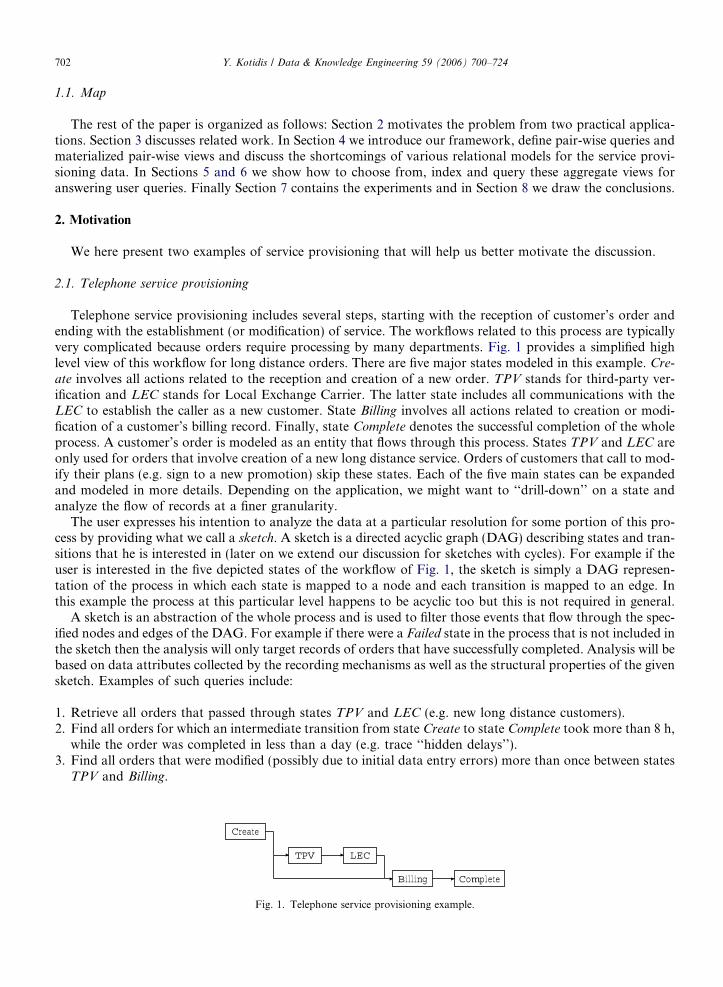
We note that all these operations can be described in the context of pair-wise aggregate queries.Hide(u): this operation results in a simpler sketch by removing node u from consideration. For a sketch

G(V,E), Hide(u) results in a new sketch G 0(V � {u},E 0) where

E0 ¼ E [ fða; bÞ : ða; uÞ; ðu; bÞ 2 Eg � ðfðu; ?Þ 2 Eg [ fð?; uÞ 2 EgÞ

Fig. 5 shows the resulting sketches from three successive calls: Hide(B) followed by Hide(D) and Hide(C).The first call removes node B from the sketch. Incoming edge (A,B) is replaced by edges (A,F), (A,C) and(A,D). Edge (A,F) ‘‘hides’’ the detailed transition A! B! F. For records that contain this transition, thetwo measures xAB and xBF are replaced by a derived measure xAF. Like the case of the UnZoom operation,the exact formula depends on the context. For instance, if the measures relay cost information, one can usexAF = xAB + xBF = sumB!F.

4.4. Processing of pair-wise queries in a relational data store

A natural attempt to store this data in a relational system is to break each record into a list of (record-id,edge-id, measure) triplets using table: Rðrid ; eid ; xÞ. This vertical representation has an excellent effect whenquerying on transitions between two adjacent nodes: a pair-wise query Fu!v, where (u,v) 2 E is efficientlycomputed given an index on eid. However, for paths u! v with one or more ‘‘hops’’ the query requires a num-ber of self-joins of R equal to the length of the path in order to ‘‘collect’’ all measures along the path. Fur-thermore, in case there are more that one paths between the selected nodes, the user has to implicitly writean SQL sub-query for each one of them. For example query sumB!D P 5 returns the union of the followingexpressions:

Hide(B)

Hide(D)

Hide(C)

A

A

A

A

B CD E

E

E

EC

F

FF

F

DC

Fig. 5. Hide operation.


q1: select R1.rid, R1.x + R2.xfrom RR1;RR2

where R1.rid = R2.rid and R1.eid = 00BC00and R2.eid = 00CD00 and R1.x + R2.x P 5

q2: select R.rid, R.xfrom RRwhere R.eid = 00BD00 and R.x P 5

An alternative horizontal representation of the data is: Rhðrid ; xe1; . . . ; xejEj Þ, where xei is the measure for edge

ei. If a record does not contain a transition, the corresponding xei value is null. Compared to the vertical rep-resentation, the horizontal schema avoids the need for self-joins, but the user is still required to implicitlydescribe all paths between the end-points u, v. The previous query is now written as

q3: select Rh.rid , Rh.xBC þRh.xCD

from Rh

where Rh.xBC þ Rh.xCD P 5q4: select Rh.rid , Rh.xBD

from Rh

where Rh.xBD P 5

A potential problem of the horizontal representation is that most commercial database systems impose alimit on the number of columns in a table that can be reached when G(V,E) is large and multiple measuresare being collected along each edge.

For aggregate functions like sum( ) and count( ) we can exploit a dual prefix-representation [22,29] of therecord:

rdF ¼ fðv

e11 ; 0Þ; ðv

e21 ;Fðx1ÞÞ; . . . ; ðvekr

1 ;Fðx1; . . . ; xkr�1ÞÞ; ðvekr2 ;Fðx1; . . . ; xkrÞÞg ð3Þ

The prefix-F representation allows us to compute the aggregation by subtracting the prefix-representation ofthe measure at the ending node from the prefix-representation at the starting node using table Rd

Fðrid ; vid ; xFÞ.Thus, a pair-wise query sumu!v/countu!v is expressed as a single self-join that can be optimized using an indexon the vid column.

For example sumB!D P 5 is written as

q5: select R1.rid, R2.xsum � R1.xsum

from RdsumR1;R

dsumR2

where R1.rid = R2.rid

and R1.vid = 00B00 and R2.vid = 00D00and R2.xsum � R1.xsum P 5

A common restriction of all three representations is that, in many cases, we cannot use an index for thepredicate on the measures (e.g. queries q1, q3 and q5). If the predicates on the measures based on values l,h are highly selective (which is the case when we are looking for outliers) indexing on the path informationthrough indexes on eid or vid will not be sufficient. Querying the dataset is also cumbersome for the user, asshe/he has to compose the query appropriately to reflect the part of the sketch that is interested in. Material-ized views can be used to accelerate query performance and also ease navigation through the dataset.

For some aggregate function F let view VF compute all pair-wise aggregates Fu!v for each u and v forwhich there is a path u! v in GðV ;EÞ : VF ¼ fu; v; rid ;FðP u!vðrÞÞg. Using the view it is straightforward toexpress query l 6Fu!v 6 h with selections on columns u and v. In addition to these attributes, indexes on thederived function values FðP u!vðrÞÞ can be used to accelerate retrieval of matched records. The view requires,asymptotically, OðjV j2 � jRjÞ space, where jVj is the number of nodes in the sketch and jRj the number ofrecords. The complete pair-wise collection of values in VF will probably be prohibitively large to computeand store. In the following sections we show that there is a lot of redundancy in the values of this view that


we use to reduce the space requirements. For referring to appropriate subsets of view VF we use the followingnotation.

Definition 4.5. Given a pair u, v for which there exists a path u! v in G(V,E) we define view VFu!v as theprojection of all records in VF that contain these states.

5. Processing path queries

For a start we assume that F ¼ existð Þ, i.e. we are only interested in the transitions stored in the recordsand not in the actual measures. A pair-wise path query existu!v = 1 retrieves all records that include a pathfrom u to v.2 View Vexistu!v lists all records that are returned by that query. The view can be stored as a listof record-ids or even better as a (compressed) bitmap of length jRj.

Definition 5.1. Vexistu!v is a bitmap of length jRj with bits set at position i, for every record ri 2 Su!vðRÞ.

Given that Vexistu!v is materialized, what other queries benefit from this view? The answer to this question isencoded in the graph representation of the sketch. Assume for instance that view VexistC!E is materialized. Thisview lists all records that contain a path C! E. Since this path always includes state D we conclude thatSC!DðRÞ ¼ SC!EðRÞ and therefore we can use this view to answer query existC!D. For the previous query,materialized view VexistB!D contains a superset of the required records since SC!DðRÞ � SB!DðRÞ. As a result,querying the view instead of R results in generating false positives, i.e. it will return additional records that donot belong to SC!DðRÞ. However, one might want to use the view, as a dirty filter over the dataset if the num-ber of bits set in VexistB!D is much less than jRj, e.g. when lots of events terminate on state F. A third choicearises for query existD!E and view VexistC!E . Because of edge (B,D), using the view to answer this query resultsin false negatives, i.e. dismissal of records that contain the requested transition. An answering mechanism thatrequires no false dismissals should always avoid the last case.

5.1. Materialized views for pair-wise path queries

We now investigate the problem of selecting the minimum subset of views Vexistu!v to be materialized so thatsubsequent pair-wise path queries can be answered from these views without accessing the dataset. We firstdefine the notion of equivalence among two views.

Definition 5.2. Given two pairs of nodes (x,y) and (a,b) s.t. there is a path from x to y and from a to b inG(V,E) we say that Vexista!b is equivalent (�) to view Vexistx!y if they contain the same records for any instanceof R.

The definition implies that Vexista!b �Vexistx!y if each valid record that contains a path x! y also containsa path a! b and vice-versa. This means that there is a path x! a or a! x in G(V,E). Assuming that the firstis true (otherwise we swap (x,y) and (a,b)) the following condition verifies that x is always included in a recordthat contains a path a! b:

1. For all nodes s in the set of starting nodes of G(V � {x},E � Ex),3 9= a path s! a.
Depending on the relative position of the remaining nodes in the sketch we have the following cases:Case (1): $ a path y! a in G(V,E). Because the graph is acyclic, this implies that nodes a and b are reachedafter departing nodes x and y in the specified order. We denote this as: x! y! a! b. In this caseVexista!b �Vexistx!y if (i) after leaving node y we always pass through a and b and (ii) any path s! a includesy. Thus, the following additional constraints must be met:2. For all nodes t in the set of terminal nodes of G(V � {a},E � Ea), 9= a path y! t.3. For all nodes t in the set of terminal nodes of G(V � {b},E � Eb), 9= a path y! t.
2 Similarly, existu!v = 0 retrieves all records without such a transition. When the predicate is omitted, we assume it is =1.3 G(V � {v},E � Ev) is the graph obtained if we remove node v from the sketch and all its incident edges, e.g. Ev = {(v1,v2) 2 E s.t. v1 = v

OR v2 = v}.

x ay bS T

Required path

Forbidden path

Fig. 6. Required and forbidden paths in a sketch (case 1).


4. For all nodes s in the set of starting nodes of G(V � {y},E � Ey), 9= a path s! a.
Fig. 6 depicts the required and forbidden paths in a sketch for case 1 to hold. Super-nodes S and T correspondto all starting and terminal nodes.Case (2): $ a path a! y in G(V,E). We denote this as: x! a! y! b. In this case we verify conditions (1), (3)as well as:5. 9= a path x! y in G(V � {a},E � Ea).6. 9= a path a! b in G(V � {y},E � Ey).
Case (3): $ a path b! y in G(V,E). This is denoted as x! a! b! y. In this case we test conditions (1), (5) aswell as:

7. For all nodes t in the set of terminal nodes of G(V � {y},E � Ey), 9= a path b! t.8. 9= a path x! y in G(V � {b},E � Eb).

These tests require at most 2jSj + 2 Depth-First-Search scans of the graph for every pair (x,y) and (a,b). Westretch here that these tests are only performed once when the sketch is specified. For a sketch with 50 verticesand 100 edges they take 45 seconds in a 600 MHz Pentium III PC.

The � relation partitions the views in equivalent classes ~V1; ~V2; . . . In the graph of Fig. 3 we have the fol-lowing four classes:

~V1 ¼ fVexistA!C ;VexistB!C ;VexistC!D ;VexistC!Eg~V2 ¼ fVexistA!F ;VexistB!F g~V3 ¼ fVexistA!D ;VexistA!E ;VexistB!D ;VexistB!E ;VexistD!Eg~V4 ¼ fVexistA!Bg

All views belonging to the same class ~Vi contain exactly the same bitmap for any instance of R. Thus, onlyone of these views is needed to be materialized. For a view Vexistu!v , we denote as ~Vexistu!v the materializedrepresentative of its class. We also denote the number of classes of equivalent views in G(V,E) as j ~Vj. Inthe graph of Fig. 3, j ~Vj ¼ 4.

In the previous discussion we assumed that there is a path from u to v in G(V,E). If this is not true thenVexistu!v is empty by default. These views belong to a virtual class ~V0. The representative of this class containsno records. On the opposite side, when transition u! v exists in all records for any instance of R (like A! B

in our example), the corresponding view indexes the whole dataset and ~VexistA!B is not materialized. In order tosee whether the representative ~Vexistu!v of a class trivially indexes all records in R the following condition istested:

9. For all pairs s, t from the sets of starting and terminal nodes of G(V � {u,v},E � Eu � Ev), 9= path s! t.

For the sketch of our example just three representative views are needed whose combined size is 3jRj(uncompressed) bits. In practice j ~Vj depends on the complexity of the sketch. Business processes often haveparts with sequential actions v1! v2! � � � As an example processing of a customer’s order spawns severalprocesses (possibly on different departments) that are executed in parallel. We model this scenario in the fol-lowing way: starting with a set of k nodes that are lined in a chain, we pick a random non-terminal node, gen-erate a new branch from that node of length 6k and repeat several times. Fig. 7 shows a possible result for

Fig. 7. A service provisioning tree.

55 10 15 20 25 30 35 4000

55

10

15

20

25

30

# of nodes

# of

cla

sses

Fig. 8. Number of classes.


k = 5 and four iterations. Processes of this form are common in the telephone service provisioning domain. InFig. 8 we plot the number of classes j ~Vj versus the number of nodes in a sketch that we generate this way. Wevaried k between 3 and 6, generated a sample set of 100 graphs and averaged the number of classes forsketches with the same number of nodes. Clearly for this case the number of classes is linear in the numberof nodes and the combined size of all views is about the same as the size of a single index on the relation col-umn storing the edge identifiers eid (see Section 4.4). We believe this to be true in many practical cases.

5.2. Evaluating more complex path queries

We now define the selection operator Sv1!��!vnðRÞ that returns all records that visit nodes v1, . . . ,vn in thespecified order. A multi-node path query existv1!��!vn evaluates to 1 for all records in Sv1!��!vnðRÞ and is com-puted as follows:

n = 1: We answer the query by ORing the bitmaps of all views ~Vexists!v1, s 2 S. Alternatively we could use

views ~Vexistv1!t , t 2 T. Overall, we need to OR at-most minðjSj; jT j; j ~VjÞ bitmaps.n = 2: We directly answer the query using view ~Vexistv1!v2

.n > 2: We AND bitmaps of views ~Vexistvi!viþ1

; i ¼ 1; . . . ; n� 1. Up to minðn� 1; j ~VjÞ bitmaps are read. This isa crude upper bound as many of these views belong to the same class.

More complex path queries can be expressed as series of multi-node expressions. For example, if we wantall records that pass through nodes A,B,D,E but not from C we compute: existA!B!D!E AND NOTexistC!C ¼ ~VexistA!B AND ~VexistB!D AND ~VexistD!E AND NOT ~VexistA!C ¼ ~VexistA!E AND NOT ~VexistA!C .

A path query can be answered using bit-mapped indices on the nodes (B(ui)) based on the dual represen-tation of a record. There is a direct way to translate the optimized view expression to an optimized expressionof bitmaps on the nodes. For the sketch of our running example there are the following four equivalent classesof bitmaps: B(A) � B(B) (with all bits set), B(C), B(D) � B(E) and B(F). The query is now expressed as B(A)AND B(B) AND B(D) AND B(E) AND NOT BðCÞ ¼ ~BðDÞ AND NOT ~BðCÞ.


While, for a DAG, the translation to the dual representation is straightforward, in the next subsection wedemonstrate that when the sketch contains cycles, pair-wise views are more expressive than using bitmappedindexes on the state information.

5.3. Processing path queries in a digraph

A digraph G(V,E) is used as a sketch if each weakly connected component has a non-empty set S 0 2 V ofnodes with no incoming edges and a non-empty set T 0 2 V of nodes with no out-going edges. The definition ofa record is now changed to be an ordered multi-set of (edge,measure) values. Query Fu!v is defined to aggre-gate all measures between the first occurrence of node u and the last occurrence of node v in the record.4

Since the sketch may contain cycles, we need to add additional constraints in the evaluation of pairs (x,y)and (a,b) for computing the � relation.

Case (1): Constraints (1)–(4) ensure that nodes a and b are visited after nodes x, y in a record. In an acyclicgraph this is enough to guarantee a path x! y! a! b in the record. In a digraph we may also see paths:x! y! b! a, y! x! a! b and y! x! b! a that should be excluded. For that we add the followingtwo tests:

10. 9= a path y! b in G(V � {a}, E � Ea).11. For all nodes s in the set of starting nodes of G(V � {x},E � Ex), 9= a path s! y.Case (2): The relative order of the nodes cannot change if all four constraints are met.Case (3): We need to secure the order of nodes x and y with the following test:12. 9= a path x! b in G(V � {a},E � Ea)

When evaluating a multi-node path query as described in Section 5.2 the resulting bitmap describes morerecords that are actually in Sv1!��!vnðRÞ as the evaluation process does not guarantee an order between pathsvi! vi+1. For example record r ¼ f. . . ; ððv2; v3Þ; xðv2;v3ÞÞ; . . . ; ððv1; v2Þ; xðv1;v2ÞÞ; . . .g contains both a path v1! v2

and v2! v3 but not path v1! v2! v3. Such a record is possible in a (complex) digraph but not in a DAG.Thus, we use the optimized expression as a dirty filter and evaluate the retrieved records at a latter step toeliminate possible false positives.

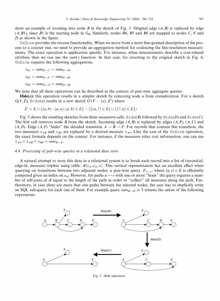
Example 5.3. For the graph of Fig. 9, the equivalent classes are:

4 Oth

~V1 ¼ fVexistA!B ;VexistA!C ;VexistA!D ;VexistB!C ;VexistB!D ;VexistC!Dg~V2 ¼ fVexistA!E ;VexistB!E ;VexistC!E ;VexistD!Eg~V3 ¼ fVexistA!F ;VexistB!F ;VexistC!F ;VexistD!F g~V4 ¼ fVexistD!B ;VexistD!C ;VexistC!Bg

The representative of class ~V1 is omitted because of condition (9). Suppose that we want to find all recordsthat used the back-edge (D,B) and terminate at node E. The query is formulated as: existA!D!B!E. We com-pute ~VexistA!D AND ~VexistD!B AND ~VexistB!E = ~VexistD!B AND ~VexistB!E . It is easy to see that for the given sketch,the result describes exactly the records that we want, i.e. there are no false positives. Processing requiresretrieving exactly 2 bitmaps.

If for the same query we were to use bitmaps B(ui) on the nodes we get: B(A) AND B(B) AND B(D) ANDB(E) = B(E). This expressions describes all records that terminate on node E whether or not they used theback-edge (B,D) and there is no way to express this property using indexes on the nodes. Pair-wise viewson the other hand allow us to describe arbitrary transitions between two nodes but evaluation does not guar-antee the order of consecutive pairs in the expression. Compared to using bitmapped indices on the nodes, wecan show the following.

er definitions are possible depending on the context.

AA BB C D E

FF

Fig. 9. Sketch with cycles.


Lemma 5.4. Evaluation of a multi-node path query existv1!��!vn in a digraph using bitmap indexes on the nodes vi

results in at least as many false positives as the optimized expression of pair-wise path views.

In many practical scenarios pair-wise views do not add false positives in evaluation of path-expressions overdigraphs. In-fact, we can detect all pathological cases by analyzing the sketch in a similar manner. That is, wecan tell if there is a need to make a second pass over the records to eliminate false positives by looking at thesketch.

6. Processing pair-wise aggregate queries

We now address the problem of using materialized views for answering pair-wise aggregate queries of theform:

5 Fu1 < i <functiopartitio

l 6Fa!b 6 h ð4Þ
when F ¼ sumð Þ; countð Þ;maxð Þ;minð Þ. A pair-wise aggregate view VFx!y contains pairs of ðrid ;FðP x!yðrÞÞÞvalues. We can implement this view as a B-tree with the second value used as a key and the first value used topoint to the appropriate records in R.
If another view VFx!y with (x,y) 5 (a,b) and Vexistx!y �Vexista!b is materialized it can be used to locate allrecords with a transition from a to b. This however is inefficient if the numeric predicates on the aggregate arehighly selective, e.g. when many records contain a path from a to b but few of them satisfy l 6FðP a!bðrÞÞ 6 h.

Unfortunately, there is no way to relate the aggregates stored in the view with the aggregates requested bythe query since pairs (x,y) and (a,b) might be on (connected but) unrelated parts of the sketch. As an exampleconsider query maxB!D > 100 that retrieves all records that either have (i) an edge (B,D) with a measuregreater than 100 or (ii) edges (B,C) and (C,D) with associated measures that at least one is greater than100. If view VmaxD!E was materialized it provides filtering on the path expression only, since VexistD!E �VexistB!D . On the other hand, view VmaxA!E provides more leverage since a candidate record r must havemax(PA!E(r)) > 100. Therefore, we execute query maxA!E > 100 on view VmaxA!E and then check theretrieved records whether max(PB!D(r)) is indeed greater than 100. This process is called query rewritingand is discussed in details in the forthcoming sections.

In general we may be able to exploit the aggregates stored in view VFx!y when evaluating query (4) if nodesa and b are contained in a path from x! y. Containment is not a mandatory condition for view equivalence asdefined in the previous section. It is described as x! a! b! y in case (3). When all four conditions for thiscase are met then for distributive aggregate functions, the stored aggregate value along path x! y can beexpressed as5:

FðP x!yðrÞÞ ¼F0ðFðP x!aðrÞÞ;FðP a!bðrÞÞ;FðP b!yðrÞÞÞ ð5Þ
where F0 ¼F for F ¼ maxð Þ;minð Þ; sumð Þ and F0 ¼ sumð Þ for F ¼ countð Þ. This well-known property of adistributive function is frequently exploited to share computation of data cube aggregates [2].
nction Fðx1; . . . ; xnÞ is distributive if there exists function G such that Fðx1; . . . ; xnÞ ¼ GðF ðx1; . . . ; xiÞ; F ðxiþ1; . . . ; xnÞÞ for any i:n. The definition implies that the input of F can be partitioned into an arbitrary number of sets (sub-problems) and the result of then can always be computed by composing (using G) the results of the sub-problems without any ‘‘state’’ information on howning were obtained.


For any two pairs of nodes (x,y) and (a,b) for which the conditions of case (3) are met we denote thatVFa!b �VFx!y . The � relation is reflexive, transitive and antisymmetric. Thus, it defines a partial orderon the views. The antisymmetry comes from the containment requirement. For the sketch of Fig. 3 the � rela-tion is shown in Fig. 10. A node in the figure represents an aggregate view on the corresponding pairs. Anarrow between two views depicts that the pointed view � the other. We also include the whole dataset Rto depict that all these views can be computed from the raw records.

For a view VFu!v the top-level ancestor, i.e. the higher view V in the hierarchy s.t. VFu!v �V is denoted

as VFu!v . For example VFD!E ¼VFA!E . The number of top-level views is denoted as jVj, and is 5 in ourexample.

6.1. Weaker condition

When view VFx!y such that VFa!b �VFx!y is used for query (4), it retrieves all records with a transitiona! b with some additional filtering based on a rewriting for the measures along x! y. The details of thisrewriting are included in the forthcoming sections. The rewriting introduces false positives (but no false neg-atives) for the aggregate values but is exact on the path requirement: all records retrieved from view VFx!y

contain a path a! b.We can relax the path equivalence requirement at the expense of getting more false positives. We define that

VFa!b �VFx!y if (i) x is required to reach a and (ii) any path from b to a terminal node includes y. Thus, onlytests (1) and (7) are required.

The � relation is also a partial order and implies that Sa!bðRÞ � Sx!yðRÞ. For the sketch of Fig. 3 the �partial order is depicted in Fig. 11. The top-level views of the order are denoted as _V and their number as j _Vj.In this example j _Vj ¼ 3.

Based of the definition of relations �, � and � the following observations are made:

• VFa!b �VFx!y implies that Vexista!b �Vexistx!y and therefore j ~Vj 6 jVj.• Views VFa!b answer exactly path queries in a DAG and with possible false positives in a digraph.

AE

AD

BD

BE

DE

CE

CD

AC

BC

AF

BF

AB

R

Fig. 10. The � partial order.

AE

AD

BD

BE

DECE

CD

AC

BC

AF

BF

AB

R

Fig. 11. The � partial order.


• VFa!b �VFx!y implies that VFa!b �VFx!y and therefore j _Vj 6 jVj.• Views _VFa!b is the smallest set of pair-wise views that answer any pair-wise path/aggregate query with no

false negatives without looking at the data. However, these views may introduce false positives in pathexpressions both in a DAG and a digraph.

6.2. Pair-wise sum-queries

Pair-wise sum-queries are queries of the form: l 6 suma!b 6 h. We assume that at least the top-level viewsVsumu!v of the � hierarchy of Fig. 10 are materialized and we explore how queries on the remaining pairs canbe translated and executed efficiently using these views.

If view Vsuma!b is not computed we are using materialized view Vsumx!y ¼ Vsuma!b as a dirty filter to findcandidate records that we retrieve and evaluate from R in a latter step. Along with the views, we store inthe database the dependency graph of Fig. 10. This graph has a size of O(jVj2), which we consider insignificantin a data warehouse context. For each node in the graph we maintain the minimum and maximum value ofthe sum( ) function evaluated over the stored records that contain the specified transition. For instance, nodeDE will store the following two numbers: min_sumD!E = min(sum(PD!E(r))) and max_sumD!E =max(sum(PD!E(r))) for all r 2 SD!EðRÞ. These statistics are easy to maintain in an append-only scenario,while we load new records in the data warehouse. In fact, many service provisioning datasets are obtainedfrom recording tools and data is indeed append only. Using Eq. (5), query l 6 suma!b 6 h is re-written as6:

6 we

l0 ¼ lþmin sumx!a þmin sumb!y 6 sumx!y 6 hþmax sumx!a þmax sumb!y ¼ h0 ð6Þ
We therefore query view Vsumx!y using constants l 0 and h 0 and get a list of rids that satisfy formula (6). Eachcandidate record r is retrieved from R in order to evaluate whether l 6 sum(Pa!b(r)) 6 h. Because of the �relation using the view is equivalent for the path-requirement a! b and is therefore at least as good as usingany type of indices on the node/edge-ids of the records.
Lemma 6.1. A query rewrite of formula (6) results in accessing no-more records than what is required because of

the path-expression a! b.

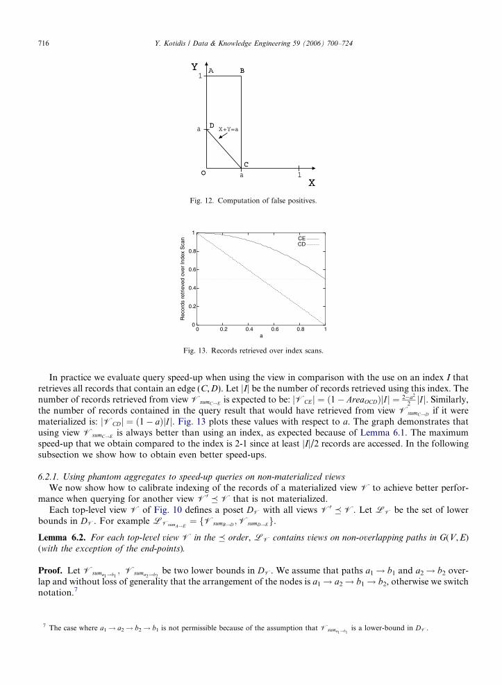
We now calculate the number of false positives introduced by the rewriting of formula (6). The probabilityof a record being a false positive is the conditional probability:

Probfalse positive ¼ ProbðsumðP a!bðrÞÞ 62 ½l; hjsumðP x!yðrÞÞ 2 ½l0; h0Þ

If the distribution of values of the stored measures are known, one can analytically compute the aboveprobability for any combination of pairs a,b and x,y. As an exercise, we here consider the following example.Assume that the values collected along edges (C,D) and (D,E) form two independent uniform random vari-ables X and Y respectively. Assume that view VsumC!E is materialized and used for evaluating query:a 6 sumC!D 6 1, i.e. the query requests all records with X P a (with a 6 1). Using formula (6) we retrieveall records with a + 0 6 X + Y 6 1 + 1, since min_sumD!E = min(Y) = 0, max_sumD!E = max(Y) = 1. Theprobability of getting a false positive is then:

Probfalse positive ¼ ProbðX < ajX þ Y P aÞ ¼ ProbðX < a ^ X þ Y P aÞProbðX þ Y P aÞ

This probability is computed based on Fig. 12. All records retrieved from the rewriting X + Y P a are aboveline DC. Thus, we must compute the integral of the join-density distribution for the trapezoid ABCD over theintegral over the whole area except the lower triangle OCD. For independent uniform random variables theintegrals simply compute the respective areas:

AreaABCD ¼ð1þ 1� aÞ � a

2;AreaOCD ¼

a2

2) Probfalse positive ¼

ð2� aÞa2� a2

assume that min_sumu!v = max_sumu!v = 0 if u = v.

a 1

X+Y=a

YY

XX

1A BB

CC

DDa

OO

Fig. 12. Computation of false positives.

0

0.2

0.4

0.6

0.8

1

0 0.2 0.4 0.6 0.8 1

Rec

ords

ret

rieve

d ov

er In

dex

Sca

n

a

CECD

Fig. 13. Records retrieved over index scans.


In practice we evaluate query speed-up when using the view in comparison with the use on an index I thatretrieves all records that contain an edge (C,D). Let jIj be the number of records retrieved using this index. Thenumber of records retrieved from view VsumC!E is expected to be: jVCEj ¼ ð1� AreaOCDÞjI j ¼ 2�a2

2jI j. Similarly,

the number of records contained in the query result that would have retrieved from view VsumC!D if it werematerialized is: jVCDj ¼ ð1� aÞjI j. Fig. 13 plots these values with respect to a. The graph demonstrates thatusing view VsumC!E is always better than using an index, as expected because of Lemma 6.1. The maximumspeed-up that we obtain compared to the index is 2-1 since at least jIj/2 records are accessed. In the followingsubsection we show how to obtain even better speed-ups.

6.2.1. Using phantom aggregates to speed-up queries on non-materialized views

We now show how to calibrate indexing of the records of a materialized view V to achieve better perfor-mance when querying for another view V0 �V that is not materialized.

Each top-level view V of Fig. 10 defines a poset DV with all views V0 �V. Let LV be the set of lowerbounds in DV. For example LVsumA!E

¼ fVsumB!D ;VsumD!Eg.

Lemma 6.2. For each top-level view V in the � order, LV contains views on non-overlapping paths in G(V,E)

(with the exception of the end-points).

Proof. Let Vsuma1!b1; Vsuma2!b2

be two lower bounds in DV. We assume that paths a1! b1 and a2! b2 over-lap and without loss of generality that the arrangement of the nodes is a1! a2! b1! b2, otherwise we switchnotation.7

7 The case where a1! a2! b2! b1 is not permissible because of the assumption that Vsuma1!b1is a lower-bound in DV.


Because of conditions (1), (5), (7) and (8) of case (3) for a1! b1 and a2! b2, we conclude thatVsuma2!b1

�V; that is Vsuma2!b12 DV. With similar arguments we have that Vsuma2!b1

�Vsuma1!b1. The latter

contradicts the assumption that Vsuma1!b1is a lower bound in DV, unless a1 = a2. However, in case (a1 = a2)

then Vsuma1!b1�Vsuma2!b2

, which again contradicts the assumption that Vsuma2!b2is a lower bound, unless

a1 = a2 and b1 = b2. That is, the two paths cannot overlap, unless we are talking about the same pair. h

Our key-idea is to use the values of the views in LV to cluster the records of V in a way that will allowfewer false positives due to the rewriting. We propose two methods for storing the view based on partitioningits records on the values of the aggregates in LV. We call these values phantom aggregates as they do notappear in V. Both methods maintain a hybrid data-structure, in which the upper part describes a partitioningscheme based on the phantom aggregates and the lower part implements a collection of B-trees on the valuesof V, using one tree per partition. The upper partitioning scheme is fixed, i.e. we make no attempt to modify itduring updates. This is not a problem as phantom aggregates have a suggestive value during query rewriting.In practice we can periodically modify the partitions when the dataset or the query workload change.

kd-tree method. For some small value B, we generate B partitions for the values of V ¼ V sumu!v in the fol-lowing manner: we treat each value of V as an jLV j-dimensional point with coordinates defined by the phan-tom sum( ) aggregates of views in LV . We then build the first logjLV jðBÞ levels of a kd-tree for these values. Thekd-tree is an extension of a binary search tree in more dimensions. The main difference is that levels of the treeare split along successive dimensions, i.e level 0 is split on the first dimension, level 1 on the second etc. Moredetails on the kd-tree can be found in [20]. In our framework, each node at level logjLV jðBÞ contains a pointerto a partition of the original values in V with all records whose phantom aggregates fall in the sub-spacespecified by the path from the root to that node in the kd-tree. Each partition is organized as a B-tree havingsum(Pu !v(r)) as the key and the corresponding rids as values. At the root of each tree we store the min_sum( )and max_sum( ) values for the partition, for each phantom aggregate.

Querying this structure for any view V0 �V is done using the top-level kd-tree nodes for pruning thesearch. Queries on values of V ignore these levels and access all the underlying B-trees. In the presence ofmultiple disks, all these trees can be efficiently searched in parallel. The space requirement for the firstlogjLVjðBÞ levels of the kd-tree is 2 * (B � 1), which fits in a single data page for small Bs.

Example 6.3. We demonstrate the creation of the hybrid structure of Fig. 14 for view VsumA!E . Each record ofthis view is a pair of (rid, sum(PA!E(r))) values. We first attach the phantom aggregates of views LVsumA!E

¼fVsumB!D ;VsumD!Eg and generate a temporary table Vtemp with attributes: rid, sum(PA!E(r)), sum(PB!D(r)),sum(PD!E(r)). We then scan Vtemp and generate a kd-tree on the sum(PB!D(r)) and sum(PD!E(r)) phantomaggregates. During this phase we also compute min_sumB!D, max_sumB!D, min_sumD!E, max_sumD!E. ForB = 16, we keep the first logjLVsumA!E

j¼2ðBÞ ¼ 4 levels of the tree and use them to partition Vtemp in a second

scan. Each partition projects the first two attributes of Vtemp and is implemented as a separate B-tree usingsum(PA!E) as the key and rid as the values indexed. Nodes of the kd-tree that split the records on the phantom

Fig. 14. Implementation of view VsumA!E .


sum(PB!D(r)) aggregates are used to prune the search space when evaluating queries: sumB!D, sumB!E andsumA!D, while nodes that split on sum(PD!E(r)) aggregates are used during sumB!E and sumD !E searches.

Grid-based method. We create a hybrid data-structure, which partitions the records of the view by super-imposing a jLVj-dimensional grid on its values. The simplest way to achieve this is to partition the aggregatesof each view V0 2LV by computing appropriate quantiles [19,37,23,25]. Multi-dimensional index loadingtechniques like [15] are also applicable. Notice that the goal is not to equi-split the tuples of the view, butto impose a partitioning scheme that will benefit the expected workload on the phantom aggregates. Afterthe grid is decided, a single B-tree on the records of V is built for each cell. Storage requirements for the grid

is jLVj � ðB1

jLV j � 1Þ þ B 6 2 � B, including the pointers to the underlying B-trees.

Example 6.4. View VsumC!E is used for queries sumC!E as well as queries sumC!D, when the latter one is notmaterialized as a view. To create the grid-based hybrid-structure, we partition the records of the view based onthe phantom sumC!D values (which we know at creation time) into B P 2 sets. This is achieved using knownstatistics on the values xCD along edge (C,D) to split the records in a way that better suits the expected sumC!D

queries. Fig. 15 shows an example where B = 4. The left sub-tree contains record-ids indexed by sumC!E

values, for which the phantom xCD measure (that is not stored in the structure) is less or equal to cd1. Thesecond tree from the left has records with xCD values in the range (cd1,cd2], while the last tree contains recordswith xCD values greater than cd3. In the header-page of each B-tree we also store the minimum and maximumvalues along edge (D,E) for the corresponding partition, which again are known when the values are loaded.

Given a query l 6 sumC!D 6 h, we access the corresponding tree for each partition that intersects the [l,h]range. Each one of these trees we query using the re-writing of formula (6) where min_sumD!E andmax_sumD!E are defined per tree. In case l (resp. h) is lower (resp. higher) than the values of the grid-points ofthe partition they are substituted accordingly.

6.3. Pair-wise count-queries

For evaluating query l 6 counta!b 6 h we first list all possible paths p1, . . . ,pk from a to b in G(V,E) withthe appropriate number of transitions. As described in Section 5.2 we can find all records that contain path pi

by accessing up to j ~Vj appropriate bitmaps. This results in a bitmap Bi for each path. The answer to the queryis then computed by ORing all bitmaps Bi. This method requires no access to the dataset R and generates nofalse positives/dismissals. The method is applicable when views VFa!b (for any function F) are available. Theanswer is similarly computed by merging appropriate lists of records ids. If views _VFa!b are used then theanswer may include false positives.

6.4. Pair-wise min/max-queries

Pair-wise max/min queries are treated similarly to the pair-wise sum queries. The rewriting in this case will be:

l0 ¼Fðl;min Fx!a;min Fb!yÞ 6Fx!y 6Fðh;max Fx!a;max Fb!yÞ ¼ h0

for F ¼ minð Þ=maxð Þ.

Fig. 15. Implementation of view VsumC!E .


6.5. Handling parallel paths

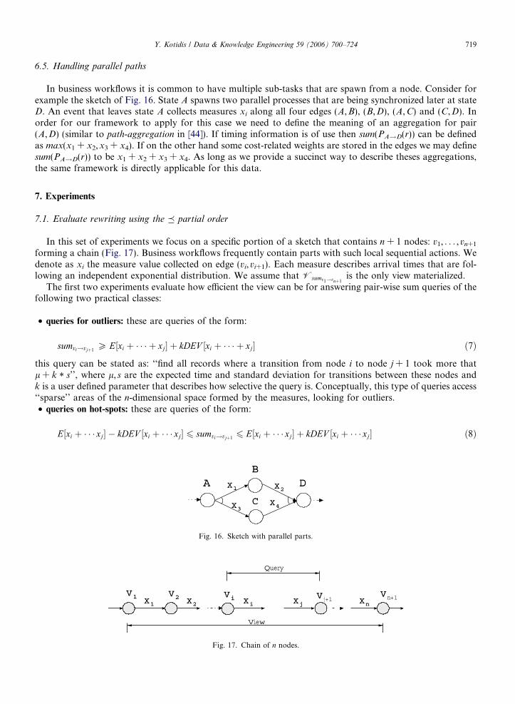
In business workflows it is common to have multiple sub-tasks that are spawn from a node. Consider forexample the sketch of Fig. 16. State A spawns two parallel processes that are being synchronized later at stateD. An event that leaves state A collects measures xi along all four edges (A,B), (B,D), (A,C) and (C,D). Inorder for our framework to apply for this case we need to define the meaning of an aggregation for pair(A,D) (similar to path-aggregation in [44]). If timing information is of use then sum(PA!D(r)) can be definedas max(x1 + x2,x3 + x4). If on the other hand some cost-related weights are stored in the edges we may definesum(PA!D(r)) to be x1 + x2 + x3 + x4. As long as we provide a succinct way to describe theses aggregations,the same framework is directly applicable for this data.

7. Experiments

7.1. Evaluate rewriting using the � partial order

In this set of experiments we focus on a specific portion of a sketch that contains n + 1 nodes: v1, . . . ,vn+1

forming a chain (Fig. 17). Business workflows frequently contain parts with such local sequential actions. Wedenote as xi the measure value collected on edge (vi,vi+1). Each measure describes arrival times that are fol-lowing an independent exponential distribution. We assume that Vsumv1!vnþ1

is the only view materialized.The first two experiments evaluate how efficient the view can be for answering pair-wise sum queries of the

following two practical classes:

• queries for outliers: these are queries of the form:

sumvi!vjþ1P E½xi þ � � � þ xj þ kDEV ½xi þ � � � þ xj ð7Þ

this query can be stated as: ‘‘find all records where a transition from node i to node j + 1 took more thatl + k * s’’, where l, s are the expected time and standard deviation for transitions between these nodes andk is a user defined parameter that describes how selective the query is. Conceptually, this type of queries access‘‘sparse’’ areas of the n-dimensional space formed by the measures, looking for outliers.• queries on hot-spots: these are queries of the form:

E½xi þ � � � xj � kDEV ½xi þ � � � xj 6 sumvi!vjþ16 E½xi þ � � � xj þ kDEV ½xi þ � � � xj ð8Þ

AABB

CC

DDXX11 XX22

XX33XX44

Fig. 16. Sketch with parallel parts.

VV11 VV22 VVii VV j+1VVn+1XX22XX11 XXii XXnnXXjj

Query

View

Fig. 17. Chain of n nodes.


These queries ask for aggregates close to the expected value of the combined distribution and evaluate therewriting when querying a ‘‘dense’’ area of the data.

For the first experiment we varied n and tested querying view Vsumv1!vnþ1for computing outliers on the first

two transitions: sumv1!v3¼ x1 þ x2 P E½x1 þ x2 þ kDEV ½x1 þ x2. We used a synthetic dataset of 1,000,000

records with a transition v1! � � � ! vn+1. In Fig. 18 we report the number of records returned from the viewvarying parameters k and n. The flat line represents the number of records returned if instead of the view we doindex look-ups in R for the two edges. This number is constant as all 1,000,000 records qualify. Two obser-vations are made from this graph: (i) performance of the view degrades with the length of the path due to‘‘noise’’ from measures x3, . . . ,xn and (ii) performance gets better when we are looking for extreme outliers(e.g. as k increases).

In Fig. 19 we experiment with queries on hot-spots using as an example query E½x1 � kDEV ½x1 6sumv1!v2

6 E½x1 þ kDEV ½x1, varying k from 0.01 to 0.30 and n from 1 (exact view) to 6. For these queries,

1 2 3 4 5 6

00

100000

200000

300000

400000

500000

600000

700000

800000

900000

1000000

Index Scan

Exact View (n=2)

n=3

n=4

n=5

n=6

k

# re

cord

s re

trie

ved

Fig. 18. Querying for outliers.

0.01 0.05 0.1 0.15 0.2 0.25 0.30

250000

500000

750000

1000000Index ScanExact View

n=2

n=3

n=4

n=5

n=6

n=2 (2 part)n=3 (2 part)

n=4 (2 part)

n=5 (2 part)

n=6 (2 part)

n=2 (3 part)

n=3 (3 part)n=4 (3 part)

n=5 (3 part)

n=6 (3 part)

k

# re

cord

s re

trie

ved

2 partitions

3 partitions

Fig. 19. Querying on hot-spots.

11 1.5 22 2.5 33 3.5 44 4.5 55 5.5 66

00

100000

200000

300000

400000

500000

600000

700000

800000

900000

1000000

Index Scan

Exact View

n=3

n=4

n=5

n=6

k

# re

cord

s re

trie

ved

Fig. 20. Pair-wise max-queries.


view Vsumv1!vnþ1is not as effective as when querying for outliers. For n > 2, the view is about as bad as using the

index. In a second run, we used the grid-based index of Section 6.2.1 with 2 and 3 partitions per phantomaggregate x2, . . . ,xn. For the first case we partitioned on the expected median of each xi, that is 0.693 for thisdistribution, and for the latter the break-points where set to 0.7 and 1.3 to better reflect the query pattern. Thesize of view Vsumv1!vnþ1

was 11.61 MB when stored as a single B-tree, 11.73 MB when stored using a

2 · 2 · 2 · 2 · 2 · 2 grid and 14.31 MB for the 3 · 3 · 3 · 3 · 3 · 3 grid.8 This is comparable to the size of aB-tree on eid (11.6 MB).

In the next experiment we evaluate processing of pair-wise max queries. Assume that we would like to findall records for which at least one transition between states v1 and v3 was delayed. Thus, we want to retrieve allrecords with an instance of x1 or x2 that was much higher than the expected value E[xi] = a. The query isstated as: query maxv1!v3

P E½xi þ kDEV ½xi. Notice how this is different than query sumv1!v3P

E½x1 þ x2 þ kDEV ½x1 þ x2 that retrieves records for which the overall transition was delayed. We evaluatedthe query using view Vmaxv1!vnþ1

, varying n from 2 (exact case) to 6. Fig. 20 plots the number of recordsretrieved. Again performance gets better when we search for extreme outliers (higher value of k).

7.2. Evaluating rewriting using the � partial order

We now modify the initial sketch by adding a cross-over edge (v1,vn+1). As a result now Vsumvi!vjþ1�

Vsumv1!vnþ1. We generated 1,000,000 new records varying the probability P of a record using the edge

(v1,vn+1). The measure along the new edge was following the same exponential distribution. We executedquery sumv1!v3

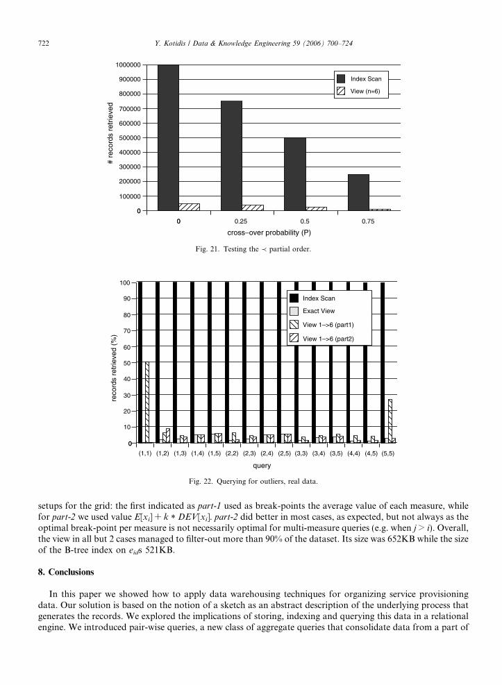
P E½x1 þ x2 þ 6 � DEV ½x1 þ x2 (for n = 6) using the view or an index on eids as shown inFig. 21. For P = 0 no record uses the cross-over path and the index returns all records. With P increasingthe index scan becomes more selective but the same is happening for the view.

7.3. Experiment with real data

For the next experiment we used real traces from a business workflow with 6 states, forming a chain. Thedataset had 42,754 records. Measures xi record timing information. In Fig. 22 we normalize the number ofrecords retrieved from view Vsumv1!v6

, those retrieved from an index on eid as well as the exact answer size, over

the dataset size for all possible queries of formula (7) with i 2 [1, 5], j 2 [i, 5] and k = 4. The x-axis in the figurerepresents pairs i, j. For the view we used a grid with 2 partitions per measure. We experimented with two

8 We also tested a grid of the form 3 · 3 · 1 · 1 · 1 · 1 that was slightly worse on queries on x1 but used only 11.62 MB of disk space.

00 0.25 0.5 0.75

00

100000

200000

300000

400000

500000

600000

700000

800000

900000

1000000

Index Scan

View (n=6)

cross−over probability (P)

# re

cord

s re

trie

ved

Fig. 21. Testing the � partial order.

(1,1) (1,2) (1,3) (1,4) (1,5) (2,2) (2,3) (2,4) (2,5) (3,3) (3,4) (3,5) (4,4) (4,5) (5,5)

00

10

20

30

40

50

60

70

80

90

100

Index Scan

Exact View

View 1–>6 (part1)

View 1–>6 (part2)

query

reco

rds

retr

ieve

d (%

)

Fig. 22. Querying for outliers, real data.


setups for the grid: the first indicated as part-1 used as break-points the average value of each measure, whilefor part-2 we used value E[xi] + k * DEV[xi]. part-2 did better in most cases, as expected, but not always as theoptimal break-point per measure is not necessarily optimal for multi-measure queries (e.g. when j > i). Overall,the view in all but 2 cases managed to filter-out more than 90% of the dataset. Its size was 652KB while the sizeof the B-tree index on eids 521KB.

8. Conclusions

In this paper we showed how to apply data warehousing techniques for organizing service provisioningdata. Our solution is based on the notion of a sketch as an abstract description of the underlying process thatgenerates the records. We explored the implications of storing, indexing and querying this data in a relationalengine. We introduced pair-wise queries, a new class of aggregate queries that consolidate data from a part of


the process, based on a user defined path expression, and explored their use for multi-resolution analysis of acomplex process through appropriate navigation operations.

We further explored the use of materialized views for speeding up frequent computations. We firstshowed how to select a minimum set of views to answer any pair-wise path query and then how to opti-mize the evaluation of more complex path-expression over the given sketch from the views. For pair-wisequeries with aggregations, we defined two partial orders among the views: � is used to find the minimumset of aggregate views to answer any query with no false dismissals while � describes an augmented set thatallows false positives on the aggregates but not on the path requirement. Computing a non-materializedaggregate is done through appropriate rewriting of the user query. We described two hybrid-indexingschemes that use phantom aggregate values and allow us to efficiently query the view, even for non-mate-rialized aggregates. Experimental results show these schemes to perform well on the synthetic and real data-sets that we used.

While our techniques have been motivated by the service provisioning scenario, our framework can beapplied to the more general problem of analyzing workflow log records generated by process managementsoftware. Post-analysis of such records can benefit from the class of aggregate queries we introduced in thispaper and our indexing and view selection techniques can further help in managing the large collections ofrecord logs generated by such systems.

References

[1] R. Agrawal, D. Gunopulos, F. Leymann, Mining process models from workflow logs, in: Proceedings of International Conference onExtending Database Technology (EDBT), March 1998, pp. 469–483.

[2] S. Agrawal, R. Agrawal, P.M. Deshpande, A. Gupta, J.F. Naughton, R. Ramakrishnan, S. Sarawagi, On the Computation ofMultidimensional Aggregates, in: Proceedings of the 22nd VLDB conference, Bombay, India, August 1996, pp. 506–521.

[3] G. Alonso, D. Agrawal, A. El Abbadi, M. Kamath, R. Gunthor, C. Mohan, Advanced transaction models in workflow contexts,in: Proceedings of the Twelfth International Conference on Data Engineering, February 1996, pp. 574–581.

[4] E. Baralis, S. Paraboschi, E. Teniente, Materialized view selection in a multidimensional database, in: Proceedings of the 23thInternational Conference on VLDB, Athens, Greece, August 1997, pp. 156–165.

[5] C. Beeri, P.A. Bernstein, N. Goodman, A model for concurrency in nested transactions systems, J. ACM 36 (2) (1989) 230–269.[6] C. Bettini, X.S. Wang, S. Jajodia, Free schedules for free agents in workflow systems, in: Proceedings of the TIME, Nova Scotia,

Canada, July 2000, pp. 31–38.[7] A. Biliris, S. Dar, N.H. Gehani, H.V. Jagadish, K. Ramamritham, Asset: a system for supporting extended transactions, in:

Proceedings of ACM SIGMOD, May 1994, pp. 44–54.[8] A. Bonifati, F. Casati, U. Dayal, M.-C. Shan, Warehousing workflow data: challenges and opportunities, in: Proceedings of VLDB,

Rome, Italy, 2001, pp. 649–652.[9] O.A. Bukhres, A.K. Elmagarmid, E. Kuhn, Implementation of the flex transaction model, IEEE Data Eng. Bull. 16 (2) (1993) 28–32.

[10] C.Y. Chan, Y. Ioannidis, Bitmap index design and evaluation, in: Proceedings of ACM SIGMOD International Conference onManagement of Data, Seattle, Washington, USA, June 1998, pp. 355–366.

[11] S. Chaudhuri, U. Dayal, An overview of data warehousing and OLAP technology, SIGMOD Record 26 (1) (1997).[12] P. Pin-Shan Chen, The entity-relationship model—towards a unified view of data, ACM Trans. Database Syst. (TODS) 1 (1) (1976)

9–36.[13] P.K. Chrysanthis, K. Ramamritham, ACTA: a framework for specifying and reasoning about transaction structure and behavior,

in: Proceedings ACM SIGMOD, May 1990, pp. 194–203.[14] J.E. Cook, A.L. Wolf, Discovering models of software processes from event-based data, ACM Trans. Softw. Eng. Methodol. 7 (3)

(1998) 215–249.[15] J. Van den Bercken, B. Seeger, P. Widmayer, A generic approach to bulk loading multidimensional index structures, in: Proceedings

of the 23rd International Conference on VLDB, Athens, Greece, August 1997, pp. 406–415.[16] J. Eder, Extending SQL with general transitive closure and extreme value selections, TKDE 2 (4) (1990).[17] J. Eder, E. Panagos, M. Rabinovich, Time constraints in workflow systems, in: CAiSE, June 1999, pp. 286–300.[18] J. Eder, G.E. Olivotto, W. Gruber, A data warehouse for workflow logs, in: EDCIS, 2002, pp. 1–15.[19] T. Feder, R. Motwani, R. Panigrahy, C. Olston, J. Widom. Computing the median with uncertainty, in: STOC, Portland, Oregon,

May 2000, pp. 602–607.[20] V. Gaede, O. Gunther, Multidimensional access methods, ACM Comput. Surveys 30 (2) (1998) 170–231.[21] H. Garcia-Molina, K. Salem, Sagas, in: Proceedings of ACM SIGMOD, May 1987, pp. 249–259.[22] S. Geffner, D. Agrawal, A. El Abbadi, T.R. Smith, Relative prefix sums: an efficient approach for querying dynamic OLAP data

cubes, in: Proceedings ICDE Conference, Sydney, Australia, March 1999, pp. 328–335.[23] A. Gilbert, Y. Kotidis, S. Muthukrishnan, M. Strauss, How to summarize the universe: dynamic maintenance of quantiles, in:

Proceedings of VLDB, 2002, pp. 454–465.


[24] J. Gray, The Benchmark Handbook for Database and Transaction Processing Systems, second ed., Morgan Kaufmann, SanFranscisco, 1993.

[25] M. Greenwald, S. Khanna, Space-efficient online computation of quantile summaries, in: Proceedings of ACM SIGMOD, 2001,pp. 58–66.

[26] D. Grigori, F. Casati, M. Castellanos, U. Dayal, M. Sayal, M.-C. Shan, Business process intelligence, Comput. Industry 53 (3) (2004)321–343.

[27] H. Gupta, Selections of views to materialize in a data warehouse, in: Proceedings of ICDT, Delphi, January 1997, pp. 98–112.[28] V. Harinarayan, A. Rajaraman, J. Ullman, Implementing data cubes efficiently, in: Proceedings of ACM SIGMOD, Montreal,

Canada, June 1996, pp. 205–216.[29] C.-T. Ho, R. Agrawal, N. Megiddo, R. Srikant, Range queries in OLAP data cubes, in: Proceedings ACM SIGMOD, Tucson,

Arizona, May 1997, pp. 73–88.[30] R. Hull, F. Llirbat, E. Siman, J. Su, G. Dong, B. Kumar, G. Zhou, Declarative workflows that support easy modification and

dynamic browsing, in: Proceedings of the International Joint Conference on Work Activities Coordination and Collaboration, 1999,pp. 69–78.

[31] H. Pirahesh, I.S. Mumick, R. Ramakrishnan, The magic of duplicates and aggregates, in: Proceedings of VLDB, August 1990,pp. 264–277.

[32] M. Kamath, K. Ramamritham, Correctness issues in workflow management, Distrib. Syst. Eng. J. 3 (4) (1996) 213–221.[33] R. Kimball, The Data Warehouse Toolkit, John Wiley & Sons, 1996.[34] Y. Kotidis, N. Roussopoulos, A case for dynamic view management, ACM Trans. Database Syst. 26 (4) (2001) 388–423.[35] P. Larson, V. Deshpande, A file structure supporting traversal recursion, in: Proceedings of ACM SIGMOD, June 1989.[36] B. List, J. Schiefer, M. Tjoa, Process-oriented requirement analysis supporting the data warehouse design process—a use case driven

approach, in: Proceedings of DEXA, September 2000, pp. 593–603.[37] G.S. Manku, S. Rajagopalan, B.G. Lindsay, Approximate medians and other quantiles in one pass and with limited memory, in:

Proceedings of the ACM SIGMOD International Conference on Management of Data, Seattle, Washington, June 1998, pp. 426–435.[38] C. Mohan, G. Alonso, R. Gunthor, M. Kamath, Exotica: a research perspective on workflow management systems, IEEE Data Eng.

Bull. 18 (1) (1995) 19–26.[39] J. Moss, Nested transactions: an approach to reliable computing. Ph.D. thesis, MIT, Cambridge, MA, 1981.[40] S.B. Navathe, Evolution of data modeling for databases, Commun. ACM 35 (9) (1992) 112–123.[41] P. O’Neil, G. Graefe, Multi-table joins through bitmapped join indices, SIGMOD Record 24 (3) (1995) 8–11.[42] P. O’Neil, D. Quass, Improved query performance with variant indexes, in: Proceedings of the ACM SIGMOD International

Conference on Management of Data, Tucson, Arizona, May 1997, pp. 38–49.[43] S. Ozeki, N. Ikeuchi, Customer service evaluation in the telephone service provisioning process, in: Proceedings of Winter Simulation

Conference, Arlington, Virginia, December 1992, pp. 1341–1348.[44] A. Rosenthal, S. Heiler, U. Dayal, F. Manola, Traversal recursion: a practical approach to supporting recursive applications, in:

Proceedings of ACM SIGMOD, 1986.[45] P. Scheuermann, J. Shim, R. Vingralek, WATCHMAN: A data warehouse intelligent cache manager, in: Proceedings of the 22nd

VLDB Conference, Bombay, India, September 1996, pp. 51–62.[46] J. Shim, P. Scheuermann, R. Vingralek, Dynamic caching of query results for decision support systems, in: it SSDBM, Cleveland,

Ohio, July 1999, pp. 254–263.[47] A. Shukla, P.M. Deshpande, J.F. Naughton, Materialized view selection for multidimensional datasets, in: Proceedings of the 24th

VLDB Conference, New York City, New York, August 1998, pp. 488–499.[48] J.R. Smith, C. Li, V. Castelli, A. Jhingran, Dynamic assembly of views in data cubes. in: Proceedings of the Symposium on Principles

of Database Systems (PODS), Seattle, Washington, June 1998, pp. 274–283.[49] S. Sudarshan, R. Ramakrishnan, Aggregation and relevance in deductive databases, in: Proceedings of VLDB, Barcelona, Spain,

1991, pp. 501–511.[50] M. Wu, A.P. Buchmann, Encoded bitmap indexing for data warehouses, in: Proceedings of the Fourteenth ICDE Conference,

Orlando, Florida, February 1998, pp. 220–230.

Yannis Kotidis is a Senior Technical Specialist at the Database Research Department of AT&T Labs-Research inFlorham Park, New Jersey. He holds an B.Sc. degree in Electrical Engineering and Computer Science from theNational Technical University of Athens and a Ph.D in Computer Science from the University of Maryland. Hisinterests include data warehousing, approximate query processing, data quality in large datasets and sensornetworks.

extending the data warehouse for service provisioning data … · · 2008-03-20extending the data...

Documents