EXTENSION BETWEEN MAJOR FAULTS,

CENTRAL OREGON BASIN AND RANGE

by

ANUWAT TREEROTCHANANON

A THESIS

Presented to the Geological Sciencesand the Graduate School ofthe University of Oregon

in partial fulfillment ofthe requirementsfor the degree of

Master of Science

September 2009

11

"Extension between Major Faults, Central Oregon Basin and Range," a thesis prepared

by Anuwat Treerotchananon in partial fulfillment of the requirements for the Master of

Science degree in the Department of Geological Sciences. This thesis has been approved

and accepted by:

II, Chair of the Examining Committee

Committee in Charge:

Accepted by:

Dr. Ray Weldon, ChairDr. David SchmidtDr. Marli Miller

Dean ofthe Graduate School

111

An Abstract of the Thesis of

Anuwat Treerotchananon for the degree of Master of Science

in the Department of Geological Sciences to be taken September 2009

Title: EXTENSION BETWEEN MAJOR FAULTS, CENTRAL OREGON BASIN

AND RANGE

Approved: -- -==o-_Dr. Ray J. Weldon II

I present an alternative approach to determine the magnitude and direction of

extension in the Basin and Range Province at the north end of Summer Lake basin using

GIS techniques. Offset across 161 faults and tilting of 56 fault blocks were estimated to

calculate extension as a function of azimuth in this area. The orientation of a

representative set of slickenlines was collected in the field to assign average values for

the GIS analysis.

Azimuthal variation ofextension is consistent with a strain ellipse indicating plane

strain with extension of 1.5 to 5.5 percent along the maximum extension direction ofN75E

and no extension along the minimum N15W axis. Blocks tilt on average 60° from the

maximum extension direction, suggesting the underlying detachment dips ~N15E. This

technique allows strain associated with the numerous small faults to be added to the sparse

large faults for a complete regional analysis.

CURRICULUM VITAE

NAME OF AUTHOR: Anuwat Treerotchananon

PLACE OF BIRTH: Chiang Mai, Thailand

DATE OF BIRTH: August 28,1979

GRADUATE AND UNDERGRADUATE SCHOOLS ATTENDED:

University ofOregonChiang Mai University

DEGREES AWARDED:

Master of Science, Geological Sciences, 2009, University of OregonBachelor of Science in Geology, 2003, Chiang Mai University

AREAS OF SPECIAL INTEREST:

Structural Geology

PROFESSIONAL EXPERIENCE:

Geologist, Siam Minerals Commercial Co., Ltd., 2004

Geologist, Petroleum Assessment Group, Bureau of Petroleum Technologies,Department ofMineral Fuels, 2003-2004

Geologist, Environmental Geology and Geohazard Division, Department ofMineral Resources, 2003

GRANTS, AWARDS AND HONORS:

Thai Government Science and Technology Scholarship, 2004

IV

ACKNOWLEDGMENTS

The completion of this project has received great support from many people

whom I'm very grateful to. First of all, I would like to deeply thank Ray Weldon, my

academic advisor for your great advice, your understanding and all your support. I'm

very indebted to you. I also would like to thank David Schmidt, a committee member and

secondary advisor, Kathy Cashman and Marli Miller for all helpful suggestions and

comments.

Special thanks to Reed Burgette and Sean Bemis for being such good and

supportive friends and office-mates, who always give me an excellent help during my

study. I would like to thank Royal Thai Government for offering me a scholarship. This

provided me a great chance to study in the United States, to gain more knowledge and

experience to widen my view.

Finally, I'm very grateful to my family for their great support. I must say that

encouragement from my family has been an important drive to lift me up and give me

energy to overcome all difficulties.

Thank you all ofyou very much indeed.

v

VI

TABLE OF CONTENTS

Chapter

I. INTRODUCTION .

Page

Location and Access.......................................................................................... 2

Geologic Setting and Background...................................................................... 4

Basic Concept.................................................................................................... 10

Extension Directions and Amounts.................................................................... 14

II. METHODOLOGy........ 19

Data Collection and Map Construction 19

Reprojecting and Combining the Layers............................................................ 22

Creating 3D Curvature Maps............................................................................. 24

Tracing Beds and the Top and Bottom ofFault Scarps....................................... 24

Breaking Faults into Pieces and Relating Points on Top and Bottom of Scarps .. 26

Detennining Area, Tilt Direction and Amount ofTilt from Each Block 30

Fitting a Best-Fit Plane to 3D Georeferenced Data................................. 30

III. RESULT AND DISCUSSION 36

Extension Direction........................................................................................... 44

Magnitude ofExtension........................................... 46

Tilted Fault Blocks 48

VB

Chapter Page

APPENDICES 54

A. FITTING AN ELLIPSE TO DETERMINE ADDED AREA......................... 54

B. APPROXIMATED AREAS FROM FITTING ELLIPSE.............................. 56

REFERENCES 58

V111

LIST OF FIGURES

Figure Page

1.1 Map of Oregon Showing Location ofthe Summer Lake Area.......................... 3

1.2 Location of the Study Area at the North End of Summer Lake Basin 3

1.3 Exposure of a Typical Fault Bounded Tilt Block in Study Area. 4

1.4 Simplified Map of the Fault Pattern Northeast of Summer Lake, Oregon......... 6

1.5 General Models ofBasin and Range Structure................................................. 7

1.6 Clay Cake Experiment Illustrating Lengthening in the Directionof Stretching. 11

1.7 Geometry of Strain Ellipse under Plane Strain. 14

1.8 Schematic Model Showing Extension of Planar Faults andDetachment Faults 15

1.9 Simple Cross Section across a Scarp................................................................ 16

1.10 Closed Crack in a Circle Making an Ellipse under Plane Strain...... 17

2.1 Index ofDEMs................................................................................................ 21

2.2 Selection ofTool and Toolset in Data Management Toolbox andDialogue Box for Reprojection ofLayers..................................................... 23

2.3 Selection ofTool and Toolset in 3D Analyst Toolbox and Dialogue Boxto Create Curvature Maps............................................................................ 24

2.4 Creating the New Shapefile in ArcCatalog....................................................... 25

2.5 The Curvature Map in the Southwest Part of the Study Area............................ 27

IX

Figure Page

2.6 The Layers ofLava Flows 27

2.7 Fault scarps are digitized in polygons to calculate expanded area..................... 28

2.8 Diagram Shows nearest Point in Nearest Point Analysis 29

2.9 Angle Convention from Nearest Point Analysis............................................... 29

2.10 Trend Dialogue in 3D Analyst Tools Box........................................................ 31

2.11 Elevation Trend ofSe1ected Surface 33

2.12 Slope Dialogue and Parameter in 3D Analyst Tools Box 34

2.13 IdentifY Cursor Tool Showing Surface Slope of Selected Area.. 34

2.14 Result from 'Trend' Command or Best-Fit Plane Comparing withCalculated Aspect 35

3.1 161 Fault Scarps and 56 Fault Blocks at the North End ofSummer Lake Basin.... 37

3.2 625 Faults and Fault Segments Plotted at 10 Intervals 38

3.3 Rose Diagram from Nearest Point Analysis Illustrates ENE-WSWAzimuthal Distribution of the Offset Vectors............................................... 38

3.4 Location ofRepresentative Orientation ofFaults and SlickenlinesCollected from the Field. 41

3.5 The Outcrop at Location#2 Showing Faults and Associate Striae..................... 41

3.6 Stereonets ofRepresentative Faults and Slickenlines in Study Area................. 42

3.7 Stereonets ofFaults and Slickenlines Broken into 3 Distinct Groups................ 43

3.8 Azimuthal Variation of the Offsets for Individual Fault 45

3.9 Azimuthal Distribution of Offsets.................................................................... 46

3.10 Aspect ofTilted Fault Blocks 51

x

Figure Page

3.11 Estimated Extension Using Added Area Approach Comparedwith an Ellipse with the Same Area.............................................................. 52

3.12 Strain Ellipse Fitting Using Least Squares Method 53

Xl

LIST OF TABLES

Table Page

1. Orientation of a Representative Faults and SlickenlinesMeasured from the Field. 40

2. Estimated Strain of the Study Area.................................................................... 49

3. Comparing Amount ofTilt Obtained from Basalt Bed and Surface Slope .......... 50

1

CHAPTER I

INTRODUCTION

The Basin and Range Province has been studied for decades. Elongated mountain

ranges and parallel basins are the result of tectonic stretching of the earth crust, resulting

in an increase in surface area. Its unique characteristics attracted many geologists to

investigate it with a variety of approaches. Although the characteristics, mechanism and

style of extension in the Basin and Range Province are known from these studies, some

topics, such as the kinematics ofvariable fault orientations and block tilts are still

controversial.

The Basin and Range Province, central Oregon, is surrounded by and includes

many zones 0 f active faults (Pezzopane and & Weldon, 1993; Weldon et aI., 2003).

Mapped patterns ofnormal fault linkages near Summer Lake show a systematic

relationship between echelon step-sense, oblique-slip sense, and the position oflinking

faults (Crider, 2001). There has been long debate about the actual kinematics of fault

displacement in this area ofvariable fault orientations and block tilts. The purpose of this

study is to determine the magnitude and direction of extension in a particularly well

exposed portion of the Central Oregon Basin and Range, and to develop a technique that

can be efficiently applied to a large set of faults with a wide range ofoffsets and

orientations. This will be accomplished by measuring the offset across faults and

characterizing the tilting of fault blocks at the north end of Summer Lake Basin in south-

2

central Oregon using GIS techniques calibrated and tested by targeted field

investigations. GIS allows the rapid characterization of a significant sample of the

numerous, well-exposed faults in the area, and field investigations provide high quality

data in selected regions to guide and validate the more extensive and easily generated

GIS data set.

Location and Access

The Summer Lake basin is located in the northwestern comer ofthe Basin and

Range Province in south-central Oregon at the center ofLake County. The study area is a

region of extensional faulting (Donath, 1962; Donath & Kuo, 1962; Lawrence, 1976;

Travis, 1977; Stewart, 1980; Zoback et.al., 1981; Pezzopane & Weldon, 1993; Crider,

2001; Badger & Watters, 2004) spanning approximately 385 km2 between the north end

of Summer Lake basin and the southern edge ofFort Rock Valley (Figure 1.1 and 1.2).

The area appears on the bottom half of the Christmas Valley 30x60 minute quadrangle

(1:1 OO,OOO-scale) topographic map produced by the United States Geological Survey,

1986.

The region provides excellent exposure ofblock-faulted, gently-dipping Pliocene

volcanic rocks that can be inferred to have been initially flat lying, and are essentially

uneroded or buried subsequent to deformation (Figure 1.3). Thus it has attracted

considerable attention (Donath, 1962; Donath & Kuo, 1962; Lawrence, 1976; Travis,

1977; Stewart, 1980; Pezzopane & Weldon, 1993; Crider & Pollard 1998; Crider, 2001;

Badger & Watters, 2004) and offers a unique opportunity to apply GIS techniques to

characterizing the deformation.

3

•Eugene

Bend·

•~ ",,"" ,"" I-nllr,!'r-\------"-"'----,.-----"--

Figure 1.1. Map of Oregonshowing location of SummerLake area (red).

Figure 1.2. The location of the study area at the north end of Summer Lake basin.Dark lines are fault scarps and the intervening regions are tilted blocks of late Miocene toPliocene largely basaltic volcanics.

4

Access is from Highway 31 that runs from U.S. Route 97 near the town of La

Pine (south of Bend, Figure 1.1) to Lakeview (east of Klamath Falls, Figure 1.1) along

western side of the study area. Good dirt and gravel roads such as County Highway 4-16

and Shuffield Road (Co Hwy 4-16A) only serve the northern part of Summer Lake

Valley. Fair to very poor gravel roads are used to access the hilly area beyond Summer

Lake Valley. Some sections ofstudy area are difficult to reach due to inaccessible roads

and private landownership.

Figure 1.3. Exposure of a typical fault bounded tilt block, Klippel Point, in study area.The block dips gently west and has a steep east-facing escarpment. Photo looks north.

Geologic Setting and Background

Basin and Range structure of this region was first recognized by John Newberry

(1855) and was explored in 1870s-1890s by railroad companies and USGS geologists.

5

The study area is covered by a sequence ofTertiary volcanic rocks greater than 2000 m

thick. The rocks are primarily basaltic and andesitic flows, interbedded with pyroclastic

tuff and minor lacustrine sediments (Crider, 2001). Most ofthe area above the valley

floor level is covered by the Pliocene Picture Rock Basalt (Travis, 1977) and older

volcanics are only seen on the lower faces of fault scarps.

Regional fault structures show a broad range in strike, length, displacement, and

degree of connectedness. Commonly the faults strike north-south, north-northwest, and

north-northeast (Figure 1.2 and 1.4). Pezzopane and Weldon (1993) recognized the north­

northwest striking faults are more numerous, generally shorter, and have less throw than

those that strike north-northeast, which have greater throw along fewer yet longer faults.

Fault throw is responsible for vertical relief in the region that ranges from a couple of

meters to as many as several hundred meters. Winter Rim and Abert Rim are the largest

structures in the region and show topographic reliefofmore than 750 m (Crider 2001).

The tectonic setting of the region is complex and has been interpreted in a variety

ofways. Pease (1969) and Lawrence (1976) suggest that the orientation and offset ofthe

N-NE-trending range bounding nonnal faults are controlled by northwest trending right­

lateral faults. On the contrary, Donath (1962) described the structure in the Basin and

Range Province in south-central Oregon. He claims that the structures in this area are

influenced by several great north-south tectonic depressions that fonn a rhombic fault

pattern in two principal sets -- N35 oW and N20 °E. Lawrence (1976) argued that the

strike-slip movement along these two sets was prior to and contemporaneous with the

generally later dip-slip defonnation. Similarly, rhombic fault patterns in Basin and Range

6

province have been mentioned by many authors, included Piper, Robinson, and Park

(1939) in the Harney Basin of southeastern Oregon, and Allison (1949) in south-central

Oregon. On the other hand, Hamilton and Mayers (1966) state that the fault pattern

resulted from both right-lateral shear and extension. Likewise, Pezzopane and Weldon

(1993) hypothesize oblique rifting, based on the pattern of faulting as compared to known

oblique rifts.

120'45'43·'5·-+------------------=__-..,....---,-;

~o~.. c==i2kll'll1llJ ~. II .

FORTROCKVALLEY

7

+---~-u...-----....;;...---.......-----'---+_43·0ll·0'

Figure 1.4. Simplified map of the fault pattern northeast of Summer Lake, Oregon.Faults are indicated by solid lines, tics on down-thrown side. (from Crider, 2001)

7

In addition to the fault orientations, the kinematics must explain the tilting ofthe

blocks in between. Three basic models have been suggested to describe the Basin and

Range structure: horst and graben, tilted block, and listric faulting (Figure 1.5). Stewart

(1980) examined regional tilt patterns for major range blocks within the Basin and Range

and Rio Grande Rift and identified broad regions of consistent tilt. His study reported that

regional tilt domains are compatible with the tilted block model or the listric fault model

but not the horst and graben model (Zoback et aI., 1981). The study area also can be

divided into regions with consistent tilts, suggesting variable dips on listric faults or the

detachment surfaces underneath groups of similarly tilted blocks.

(a)

horst and graben

(b)

tilted block

(el _:Z:Z==S:=S::S~!'

detachment surface listric fault

o 50km

Figure 1.5. General models ofbasin and range structure. (A) Horst and graben model.(B) Tilted block model. (C) Listric fault model. (from Zoback et aI., 1981)

8

Donath and Kuo (1962) ran a seismic-refraction profile along the northeast part of

Summer Lake Valley in February, 1957 to determine whether the fault block structure

underneath the large Quaternary basins is similar to that in the uplands area. The profile

was run along an azimuth ofN48 ° E, nearly perpendicular to the dominant structural

trend. The interpretation from their study shows a complexly faulted lower layer oriented

similarly to the upland. The dimensions of the fault blocks underneath are approximately

1800-2500 feet wide with a high velocity layer (interpreted to be volcanic unit) that

varied from 300 feet to 1100 feet in depth. The dips of the inferred faults are very steep,

dipping from 75° to 85° or greater. Vertical separations on the faults range from 200 feet

to about 800 feet. In addition, they note that the surface faults observed in this area

suggest that the majority of faults in the region may be vertical (Donath, 1962). Given the

similarity of faulting in the exposed upland areas and that inferred below the basin, it can

be concluded that the faulting in the upland area is also representative of the unexposed

faulting beneath the basin.

The complex pattern of fault scarps in the uplands region is clearly identifiable on

topographic maps and in aerial photographs. Interpretation of aerial photography

indicates that this zone consists of numerous en echelon faults. The principle fault

escarpments typically have zigzag and sharply curved traces, and appear geometrically

segmented and separated. The Late Tertiary fault strikes in the Summer Lake area have

been divided into two dominant trends which average about N35° ± 15°W and N25° ±

15°E (Pezzopane & Weldon, 1993). It is possible that the stress orientation could be

changing and one trend cross cuts the earlier, although no author has published

9

compelling evidence of one trend consistently cutting the other. In fact, in many places,

ramp and relay fault structures show a conjugate fault geometry with linked secondary

splay faults, so both trends are seen in individual fault zones that appear to form and

grow together. Such left-stepping, en echelon fault pairs are common in south-central

Oregon, in zones that trend from northeast to northwest. These fault characteristics have

been modeled to result from the sequential evolution of displacement, with continued

extension across stepping echelon normal fault segments, the faults link to form

continuous composite faults having zigzag traces (Crider, 2001).

The inferred regional horizontal extension direction is E-W to slightly ENE­

WNW (Pezzopane & Weldon, 1993; Crider, 2001). Fault sets are oriented obliquely to

extension direction. Since horizontal principal stresses (tensor components) are not

perpendicular to the faults, the tectonics may be the result of extensional stresses oblique

to fault strike, which in theory creates oblique rifting if every fault is individually

consistent with the regional stress orientation. The theoretical consequence is that left­

stepping faults that strike northeast have left-oblique normal displacement and right­

stepping faults that strike northwest have right-oblique normal displacements, all within

the same regional stress field.

Alternatively, the area could be expanding in all directions accommodated by the

orthorhombic distribution of purely normal faults (Reches, 1978). In this case, all of the

faults would be essentially normal and together they accommodate extensional strain

oriented appropriately to the regional stress, although individual faults would appear to

be inconsistent with the regional stress orientation. By measuring the slip directions on as

10

many faults as possible and attempting to add up all ofthe fault displacements and block

tilts, I will calculate the real extension direction and magnitude, and determine which of

these conceptual models best fits the data.

Basic Concept

This study investigates the magnitude ofextension in all horizontal directions and

combines them into a strain ellipse to determine the magnitude and direction ofthe net

extension. Imagine that ifwe put a circle anywhere on the ground, before the region was

deformed; after extension occurs the circle will become an ellipse (Figure 1.6).

Hans Cloos (1936) and his brother Ernst Cloos (1955) performed the simple clay

deformation experiments by putting clay cake on top of an elastic rubber sheet and then

stretching slowly and uniformly. The entire clay layer experiences the effects of the

stretching. As a result, numerous closely spaced faults and fault scarps are developed

(Figure 1.6). The clay cake shows lengthening in the direction ofstretching, some fault

traces are straight while others are curved, typically into high angle to the direction of

extension (not clearly seen in the cartoon in Figure 1.6). Antithetic faults and a series of

tilted fault blocks have been found similar to natural patterns in the study area. In order to

get total extension, all extensions due to all faults as well as the area increased by tilted

fault blocks have to be added up. With significantly large sample of faults and block tilts,

the strain ellipse can be constructed.

11

Figure 1.6. Clay cake experiment shows lengthening in the direction of stretching.(A) Clay cake on the rubber sheet. (B) After the rubber sheet has been stretched, thecircles are deformed to an ellipse. (from Cloos, 1955)

It is assumed that all portions of the area under consideration experiences the

same stretching. It does not matter what shape the area is. As long as a circle of the same

size as the area being considered would catch the same number of faults, the location and

the shape of the sampled area is not important. We can take any representative area or

sum of areas of different shapes and calculate the size of a circle with the same area and

catch the same amount of strain that a circle of that size would catch. As the area extends,

the circle becomes an ellipse (Figure 1.7) that can be interpreted as a strain ellipse. The

12

maximum direction of the extension is the azimuth of the major axis of the ellipse. The

minor axis will be the direction of least extension. If the minor axis is the same length as

the radius of the initial circle (as shown in Figure 1.7), the region will have experienced

no extension in that direction and thus we will have plane strain, i.e. vertical thinning =

horizontal extension and no change in the 3rd dimension.

The area under consideration is called Ae, the expanded area. This is the

representative area that has been stretched and can be measured on the map. All of the

new area made is made by extension. The maximum direction of extension is the azimuth

of the major axis of our ellipse. The original area, Ao, is the area of our initial undeformed

hypothetical circle that will become the expanded ellipse.

The current area, the area of ellipse, is '!rab and the area of the original circle is

'!ra2• And if there is no extension in its short direction (as we will show below), a in the

original circle equals a, the short axis in the ellipse. The expanded area minus the original

area is the area added by extension. We called that "area added", Aa• We know the

expanded area, Ae, because it is the area today, and we can calculate the area added, Aa,

by adding up all of the area added by faults and block tilts. Using the difference between

these we can solve for the original area, and then solve for the major (b) axis. Ifwe know

how long it is, we can calculate the percent strain using the formula;

Ae- Ao = Aa = area added by extension

= 7mb - 7m2

Aa = 7m( b - a ) ------------------ (1)

13

where a is the radius oforiginal circle which we can find by taking area considered minus

area added.

------------------ (2)

:. a ~~A.:A"

The difference between major and minor axis of the strain ellipse, b-a, is the area added

by extension divided by the radius of the original area times 7r, Aa and the length of b is1m

this value plus a.

To determine the total extension, we must add up the extension from each fault.

The amount of extension depends upon I) vertical separation across the fault, 2) the dip

of the fault and 3) whether the dip changes with depth; i.e. whether the fault becomes

listric. Ifthe fault curves with depth, the extension approaches the displacement across

the fault, rather than the horizontal component of slip for a planar fault (Figure 1.8). In

theory one can relate the amount of curvature to the displacement and tilt of the

hangingwall block, and I attempted to do this by characterizing the tilt of all of the

blocks. However, we found that the tilt direction of the blocks was not in the same

direction as the slip on the faults, so the problem is quite complex. Thus we decided to

14

bracket the extension by considering 2 end members, extension associated with all planar

faults and listric faults that curve to a horizontal dip (Figure 1.8). In other words, by using

the horizontal component of extension across each planar t~lUlt yields the minimum strain

and if we use the offset across the fault it will give us the maximum value (Figure 1.8).

We attempted to compare the amount of tilting of the blocks, estimated by tracing marker

beds within blocks or by calculating the surface slope of blocks, with the extension, as

will be discussed in detail below, but did not end up using it in the strain calculations.

~--

A

Figure 1.7. Geometry ofstrain ellipse under plane strain. (A) The area in circlerepresents the original area. (8) After extension occurs, the circle will become an ellipse.

Extension Directions and Amounts

To determine the amount and direction of extension across each fault, the top and

the bottom of each fault scarp were digitized. Ideally, with planar layers and no

mod ification the vertical component of slip would be the height difference between the

top and bottom and the horizontal component would be the distance between the top and

the bottom of the scarp. However, since all fault scarps of the area have been modified by

collapse and erosion, top and bottom of scarps will have migrated back from the fault

15

A1

8

A2

e~

82

Figure 1.8. Schematic model shows an extension of each fault. A) With planar faults,extension is horizontal component of slip (eh) on faults. B) With detachment faults,extension is equal to the offset (eo) on faults.

(Figure 1. 9) and the dip of fault must be known or inferred to calculate the true vertical

and horizontal displacements. Since the dip of every fault cannot be observed, I collected

a representative set offault dips from the field to get an average value that was used to

calculate the amount of extension for each fault (Figure 1.9). This field data will be

discussed below in Chapter 3.

16

Top of carpA

bottom of s rp

A'

Figure 1.9. Simple cross section across a scarp. Top and bottom of fault scarp will betraced to get the extension.

In addition, we need to assign an extension direction for each fault or each fault

segment, if we believe slip varies as the trend of the fault varies. As discussed in detail

below in the results section, we found that slickenlines for an of the exposed fault planes

record essentially pure dip slip motion regardless of their strike, so we assume that on

average the slip direction is down dip for all of the faults. Thus the direction of extension

is estimated by breaking the fault scarp into pieces (because the faults are not straight)

and use the average dip of faults in the area to estimate amount of slip for each piece. We

can determine how much slip occurs across each piece and infer whether the slip

direction is perpendicular to that fault segment's strike. Each upper and lower fault trace

was broken into 10 meter long sections and each section was converted into its central

point (Figure 1.10). The nearest distance and direction between each top and bottom

point is measured as wen as the area, tilt direction and amount of tilt from each block,

separated by the faults. From an of these pieces we make a histogram of the amount of

extension as a function ofdirection, in 10 degree increments, by adding up an the

different pieces for each direction. With these data we can calculate the strain and

17

A

Top

B

I1

Top I J BottomI

~,I .,I \, \\ \.-- .\ ,

•\ ,"' lIr\'..------ \. .

\ '.'.~\\....-- \

"' ,, !I •

I iI .', .'

I ....'. ,I ,

I~..f'

Figure 1.10. (Top) A. Closed crack in a circle. B. expanded crack making an ellipseunder plane strain. (Bottom) Each fault scarp in the area is divided into 1O-meter longpieces. The nearest top-bottom distance for each point is measured.

18

determine the direction of extension from the histogram as well as the magnitude of

extension from added area occupied by faults and tilted blocks. The maximum value in

the frequency distribution ofthe offSet will show the direction of extension.

Although the magnitude and direction of extension can be estimated by adding up

all extension, some extension is hiding in between the faults either by the tilting ofblocks

or other distributed defonnation. Like the faults that we break into pieces, the size of the

block is important because the same tilt of a big block contributes more extension than a

small block.

Kautz and Sclater (1988) performed block faulting experiment using clay model,

and compared their findings with the results from McClay and Ellis (1987) which were

done on sand models. Their results suggest that 20-30% ofthe deformation was hidden or

internal. So that when we add up the extensions due to the mapped faults we need to

increase it by this amount to account to the small faults and the indiscernible internal

strain. In our model, the hidden deformation might be small faults that are too small to

map or small tilted blocks.

19

CHAPTER II

METHODOLOGY

In order to investigate the magnitude and direction of extension in the Basin and

Range Province in central Oregon, 3D data is used to find block tilts and to completely

determine slip across faults that vary in orientation and displacement along strike. This

study used ESRI's geographic information system (GIS) software ArcGIS v.9.2. The

USGS Digital Ortho Quad (DOQ) photography and Digital Elevation Model (DEM) were

used as the base for identifYing and mapping the faults and tilted fault blocks. The fault

scarps were primarily drawn on overlays of the DOQ images and the layers ofbasalt

flows (to determine tilt) were digitized from curvature maps generated from DEMs.

Data Collection and Map Construction

Digital elevation model (DEM) maps, developed from USGS 1124,000 (7.5

minute) quadrangles provided by the U.S Geological Survey, have been used to interpret

the geology in this study. These OEMs are created by interpolating the 10-foot elevation

contours with a matrix of 10 meter grid spacing in latitude and longitude. In order to

reconstruct bedding and fault orientation and to collect the data to determine fault offsets

and tilt ofblock, the topographic surface is derived from the 1O-m DEM obtained from

GeoCommunity web site, freely available on the internet (http://data.geocomm.com

/catalog/US/61056/429/group4-3.html). These DEMs are originally in the UTM NAD27

20

projection with vertical units in reference to National Geodetic Vertical Datum of 1929

(NGVD 29). In the UTM coordinate system, Earth is divided into sixty 6-degree-wide

zones between 84 degrees N and 80 degrees S. North American Datum (NAD) 1927 or

1983 is used mostly for areas in North America as a reference system. However, the State

Plane coordinate system can only be used within 50 states where states are divided into

small zones based on political boundaries.

In order to overlay one or more layers from the same or different sources in

ArcMap simultaneously, it is important to have all the data in the same coordinate system.

For instance, a layer in State Plane coordinate system cannot be overlain with a layer in the

UTM coordinate system. However, one can reproject the layer in State Plane into UTM

coordinate system or UTM to State Plane system, since UTM is in metric system (in

meters) and State Plane is in US metric system (in feet). The DEMs data ofthe study area

are in UTM zone ION that were reprojected to Oregon Lambert projection by The Oregon

Geographic Information Council (OGIC)'s standard. The included DEMs are (see Figure

2.1 for their locations);

Saint Patrick Mountain, OR (43120a5)

Sheeplick Draw, OR (43120a6)

Egli Rim, OR (43120a7)

Duncan Reservoir, OR (43120a8)

Fandango Canyon, OR (43120b5)

Christmas Valley, OR (43120b6)

Thorn Lake, OR (43120b7)

Tuff Butte, OR (43120b8)

The Digital Ortho Quads (DOQs) are in MrSID fonnat and can be found at Oregon

Geospatial Enterprise office (GEO) web site at http://www.gis.state.or.us/data/

21

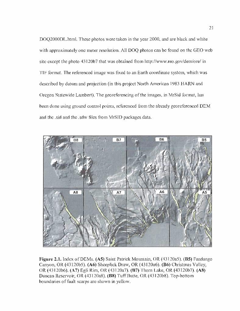
DOQ2000DL.html. These photos were taken in the year 2000, and are black and white

with approximately one meter resolution. All DOQ photos can be found on the GEO web

site except the photo 43120b7 that was obtained ii-om http://www.reo.gov/dem/ore/ in

TIF format. The referenced image was fixed to an Earth coordinate system, which was

described by datum and projection (in this project North American 1983 HARN and

Oregon Statewide Lambert). The georeferencing of the images, in MrSid format, has

been done using ground control points, referenced from the already georeferenced DEM

and the .sid and the .sdw files fTom MrSID packages data.

Figure 2.1. Index of DEMs. (AS) Saint Patrick Mountain, OR (43120a5). (BS) FandangoCanyon, OR (43120b5). (A6) Sheeplick Draw, OR (43120a6). (B6) Christmas Valley,OR (43120b6). (A7) Egli Rim, OR (43120a7). (87) Thorn Lake, OR (43120b7). (AS)Duncan Reservoir, OR (43120a8). (BS) Tuff Butte, OR (43120b8). Top-bottomboundaries of fault scarps are shown in yellow.

22

The output of the curvature function is the second derivative of the topographic

surface (i.e., the slope of the slope). The curvature function will calculate the curvature of

a surface at each cell center. A positive curvature indicates that the surface is upwardly

convex at that cell. A negative curvature indicates that the surface is upwardly concave at

that cell. A value of zero indicates that the surface is flat (ESRI, 2007). The curvature

function allows us to easily recognize and digitize beds ofbasalt flows along the

continuous convex and concave lines.

Reprojecting and Combining the Layers

The coordinate system of the DOQ photos (HARN Oregon Statewide Lambert

Feet International and in North American Datum 1983) are reprojected into HARN

Oregon Statewide Lambert (metric system) by using the "Project" tool under the

projection and transformation toolset in the Data management toolbox.

In the Project dialogue box, click the ftrst 1161icon to put the data which we

wanted to reproject then clicking the second 1(6

) icon to select the output location of

reprojected data. Finally, we selected the coordinate system in which the data is

reprojected by clicking the ~= Iicon. All the coordinate and projection information of

shapefile are stored in text file with .plj extension (Figure 2.2).

23

Input raster

G:\GIS Work\DOQ\t~3120a7.srd

GeQ9raphic Transformation (optional)

I

Input coordinate system (optional)

I

~[

..:.1

Cancel I En'lllonments... I « Hide Help IOK

Output raster

rG:\GIS Work\DOQ\t43120a7

Output coo, dinate system

INAD_1983_HARN_O'egon_Slatewide_Lamberl

Resamphng technique (optional)

INEAREST

Output 0311 size (optional)

IO.30~8

r ProjectData r~anaaernent Tools

+ ~ Data C;mparison

+ ~ Datab-3se

+ ~ Disconnected Editing

+ ~ Distributed Geod-3t-3b-3se

+ ~ Domains

~ Fe-3ture c1-3ss

~ Features

+ ~ Fields

~ File Geod-3tabase

+ @ General

+ ~ Generalization

~ Indexes

+ ~ Joins+ ~ Layers and Table Views

- ~ Projections and Transformat

.+ ~ Feature

- ~ Raster

tI- Flip

tI- ~~Jrror

tI- Project Raster

)'- Resc-3le

tI- Rotate

tI- Shift

)'- Warp

tI- Cre,3te Custom Geograp

r Define Projection

+ ~ Raster

b Rel-3tionshlp Classes

~ Subtypes

+ ~ Table

+ ~ Topology

.+ ~ Versions..... fr;<.-, \... 1...... l-l'"t"'I ::ora

< >Favorites IInde~ I Search I ReSl.Ilts I

Figure 2.2. Selection of tool and toolset in Data management toolbox and dialogue boxfor reprojection of layers.

24

Arc Toolbox

3D Analyst Tools

.. ~ Conversion

+ b functional Surface

• ~ Raster Interpolation

• ~ Raster r'-Iath

Raster Reclass

- ~ Raster Surface

? Aspect

~ Contour

j} Contour List

~ Curvature.}} Cut/Fill

? Hillshade

~ Obs:erver Points

? Slope

". Viewshed

.. ~ Terrain

• ~ TIN C, ealion

• ~ TIN Surf aceAnalysis T0015

Cartography Tools

.. ~ Conversion TDaIs

Input raster

!G: \Thesis\DE~-I\dem_a5

utput (urvatur rt6ter

IG:\Thesis\DE~1\Curvature_a5Z factor (optional)r --Output profile curve raster (optio"",l)

rOutput plan curve raslGr (optional)

I

< I

OK Cancel I Envi'.':~~nls I, )

« Hide Help J

Figure 2.3. Selection of tool and toolset in 3D Analyst toolbox and dialogue box to createcurvature maps.

Creating 3D CurvatllD.re Maps

To create the curvature map in ArcToolbox at the 3D Ana~yst tools, select the

curvature in raster surface. In the curvature dialogue box, click the first I[31 icon to put

the raster data (DEM) from which we want to create the curvature and then click the

second I~I icon to select the output location of data. Finally, selected the Z factor = 1

(Figure 2.3).

Traced Beds and the Top and Bottom of Fault Scarps

From the curvature map, now we can see the top and bottoms of the fault scarps

and the layers of lava flows outcropping within them (Figure 2.5). The next step is

digitizing the layers oflava flows to get the tilt of blocks and the top/bottom of the fault

scarps to calculate offset and extension. A blank shapefile was first created in ArcCatalog

25

before digitizing a feature. This is done in ArcCatalog by right clicking and selecting

New> > Shape/ile. filling in an appropriate name, setting the feature type to "polyline",

editing the coordinate system to UTM NAD83 Ham Oregon Statewide Lambert, and then

adding the new shapefile to ArcMap (Figure 2.4). Layers oflava flows were digitized

iiom the curvature map to calculate their inclination of the tilting fault block (Figure 2.6)

comparing with the tilting obtained from surface slope which is easier to measure.

Results from these two methods are compared in discussion chapter (Chapter 3, Table 2).

,,---reate Hew Shapefile

I~ Eolder

t_ File GeQdatabase

._1 eersonal Geodatab.'s

<> \:.ayer ...

Q §roup Layer

..--l ;ihapefile ...

Name:

Fe."ture T.l'pe:

Spoti.,,1 Reierence

Polyline

Toolbo,"

~ ~opy Ctrl+C l--.J Arclnfo ~o,.kspace

;! QBASE Table

X. Qelete

Rename F2 "iJ CO;Lerage.,

De:,cription:

Proiected Coordinate Sysl.em:r'J arne: ~·J.6.D _1383_HARN_Oregon_::tal.ewide_L.:irnbert

GeographiC Coordinate System:r·J."me GCS North_p.rneric:an_1383_HAF:N

::: &efre~h

~ew

I").. ~ear(h ...

l2T' Propeft!es ...

tiddl '3'55 Locatol ..

.. ~ XI'tlL Document

IShow Details Edit..

Iv Coordinates will contain tv1 values:. Used to store route data.

Iv Coordinates INili contain Z '/alues. Used to store 3D data.

Cancel

Figure 2.4. Creating the new shapefile in ArcCatalog. Right click and select New> >Shapefile.

26

The top and bottom of fault scarps as well as the boundary ofthe tilted fault

blocks in the area of interest were digitized in the same manner as the layers of lava

flows. But instead of setting the feature type when creating the new shapefile to polyline

for the layers, change the feature type to "polygon" for top and bottom ofthe fault scarps.

This will allow us to calculate the area added, the expanded area occupied by faults and

tilted fault blocks (Figure 2.7).

Breaking Faults into Pieces and Relating Points on Top and Bottom of Scarps

Top and bottom boundaries of fault scarps were broken into pieces, to capture the

variability in trend and displacement along the faults. This process divides and creates a

reference point at 10 meters spacing for each fault trace. Top and bottom traced lines

must be in the same convention, i.e. north to south and west to east in this study. In case

that a line is not in that convention, it can be flipped by selecting "Modified tas~' in "Edit

Editor" toolbar and right click to get into the "Flip" menu. Each top and bottom line were

exported to a new file from selection tool and divided into 10m pieces using "Divide"

tool in Edit Editor toolbar. These reference points will be saved from start to end point

ordered in our target point feature file. At this time, the reference points are only points

along the line without xyz coordinates. So we need to assign them coordinates by using

''Data Management Tools» Features» Add.xy coordinates" for xy coordinates and

"Spatial Analyst Tools » Extraction » Extract Values to Points" for z value.

27

Figure 2.5. The curvature map in the southwest part of the study area shows thelayers oflava flows exposed on fault scarps.

Figure 2.6. The layers of lava flows (red) were digitized fi·om the curvature map.

28

Figure 2.7. Fault scarps, red on hillshade image, are digitized in polygons to calculateexpanded area generated by faulting.

Each reference point on the upper line was used to find the nearest point on the

lower line to estimate amount of slip and di.rection of extension (Figure 2.8) by using

"Analysis Tools» Proximity» Near" in ArcToolbox. In the dialog, put the top scarps

in 'Input Features' and bottom scarp in 'Near Features'. Also, the search radius needs to

be adjusted to an appropriate value for each fault.

29

InputFeature

NearFeat re

1

l:J..y Figure 2.8. Diagram shows nearest point in Nearestpoint analysis. (Figure fi.-om ESRI, 2007).

x

Angles fi'om 'Near' analysis are measured in degrees, where one degree

represents 1/360 of a circle, and fractions of a degree are represented as decimal points.

Angles are measured from 180° to -180° ; 0° to the east, 90° to the nOlth, 180° (-180° ) to

the west, and -90° to the south (Figure 2.9).

1800

-1800 West _--t---_ 00 East

_90 0 South

Figure 2.9. Angle convention from nearest point analysis. Angles are measured fi.-om180° (anticlockwise) to -180° (clockwise) from east.

30

In order to convert to azimuth, following VB script is applied in the calculate tool;

Dim newAngle As Double

newAngle = [NEAR_ANGLE] + 270

While newAngle > 360

newAngle = newAngle - 360

Wend

newAngle = 360 - newAngle

where [NEAR ANGLE] is the name ofthe field in attribute table from 'Near'

analysis result.

Finally, join the calculated result together. In the dialogue, choose "Join data from

another layer based on spatial location" and then join the upper and lower faults' attribute

tables.

Determining Area, Tilt Direction and Amount of Tilt from Each Block

Fitting a Best-Fit Plane to 3D Georeferenced Data

This procedure allows the calculation of the strike and dip of any surface or bed

for which you have a set of 3D georeferenced data points defining that surface. I start by

calculating the best-fitting plane for the selected points, and then calculating the slope

and aspect of this plane. We can also evaluate the quality of the fit for the plane through

an output ofthe Root Mean Squared (RMS) error value.

To calculate the best-fitting plane for the selected points, I individually add the

shapefiles of selected point data for each basalt flow bed. We then calculate the best-

31

fitting plane by selecting "Raster Intelpolation >> Trend" command under 3D Ana~y.st

Tools (Figure 2.10).

v

« Hide Help [

AI

·11 LSI

.,1

~

~)

OK Cancel J Environnlenls .. J

Z value field

!R.lISTER\l,\LU

Type of~gression '0 tlonal)

ILlNE.II,R

Output Rr\1S file (optior,."I)

Irms_block7 T><T

Input point features

Iblock7P

Output cell size (optional)[19.8381[3 -----------

Output raster

IG: \Thesis\Process\New\seIJloint\block",block7t

Polynomial order (optional)

1

~ Trend. ' ArcToolbox

3D Analyst Tool:,

1+· ~ Conver:::ion

.+ ~ Fur,,:tional Surface

.-. ~ Ra;.ter Interpolation

,J~ JD'oN

}~ Kriging

~ r~atural Neighbor

<7"" Spline

ifl Spline with Barrier;;

.?' Topo to Raster

<7"" Topo to Raster b'y' File

.?' Trend

~+ ~ Raster r'''1ath

1+' ~ Raster Reclass

~+I ~ Raster Surface

'+ ~ Terr.",n

+ ~ TIN Creation

,+. ~ Tm 5urfoce

1+ • Analysi::: Tools

.+ Cartogr."phy Tool:::

.+ ClJnvel'~ion Tools

+ Data Inter'Jperability Tools

.+ Dato r',1anagement Tools

+ Geocodlng Tools

+ Geostatisticol Anolyst Tools

FigUl"e 2.10. Trend dialogue in 3D Analyst Tools box.

In the Trend dialogue;

a. "Input point feature" - select the shapefile from the pull-down menu

b. "Z value field" - select the field containing Z values from the pull-down

menu (if it is a shapefile enabled to store Z value, the "shape" option on

the pulldown menu should work too).

c. "Output raster" ~ browse to where you want the file saved and give the file

a name.

32

d. "Output cell size" - the default size should be fme.

e. "Polynomial order" - should be 1.

f "Type ofregression" - keep as 'Linear'.

g. "Output RMS file" - browse to a location and name the file to save a text

file of the coefficients for the plane equation, RMS error value, and a Chi­

squared value.

And then click OK, the best-fit plane will plot under selected point on ArcMap (Figure

2.11).

To determine the dip ofthe plane:

In ArcToolbox, under 3D Analyst» Raster Suiface, select Slope (Figure

2.12).

In this dialogue:

1. "Input raster" - select your plane.

2. "Output raster" - select a name and location for your slope map.

3. "Output Measurement" - make sure this is 'Degrees'

4. Then click OK.

This will assign colors based on the value ofthe dip. There may be a fringe oflower dip

values on the edges of the plane, but by using the Identify tool and clicking in the center

of the plane, the software will tell you the appropriate dip value (Figure 2.13).

33

Figure 2.11. Elevation trend of selected surface. Color scale showing elevationtrend of the surface fiom high (dark blue) to low (pale blue).

To determine the strike of this plane:

In ArcToolbox, under 3D Ana~yst > > Raster Surface, select Aspect.

In this dialogue:

I. "Input raster" ~ select plane

2. "Output raster" - select a name and location for your aspect map.

3. Click OK.

This will assign colors based on the direction the surface is facing, which equals the dip

direction. Click on the plane with the Identify tool to obtain the dip direction value, and

subtract 90 degrees from this to convert into the strike (Figure 2. I4).

34

Output measurement (optional)[DEGREE --------..'1

Output raster

I;; \Thesis\Proces5\Ne'l,,\selyornt\block\Slope\block7_slope (3/

.Ql ArcToolbox3D Analyzt Tools

+ ~ Conversion

+ ~ Functional Surface

+ ~ Raster Interpolation

+ ~ Raster Math1+1 b Raster Reelass

- ~ Razter Surface

.J' Aspect,;f"'J. Contour

? Contour Listjlo Curvature<I) Cut/Fill

tl4.... Hill5hade

? Observer Points}'- Slope

}- Viewshed

.+ ~ Terrain

,+ ~ TIN Creation

+, ~ TIN Surface+ Analysis Tools+ Carlol:Jraph\, Tools

)'- _lope

<

Input raster

rblock7t

Z facto!Joptional)1'-- - ,--

OK Cancel Environmenls. __

>1

«Hide Help

Figure 2.12. Slope dialogue and parameter in 3D Analyst Tools box.

-.: --;- 4 .- ~ - = F ....

.,. .- ----

- block7_slope371:32.33

l-:::if block7_slope

Location: 1373,634,863·j

!~e_Id__ I Valu~e_.__IIStretched value 255IPixel value 3,713233

Figure 2.13.1dent!fy cursor tool showing surface slope of selected area.

35

o

<,'

+ block?+ block?t- blod?_il'Sp

2241 G775- block7_ slope

3713233+ hs_a7

~t~:.:rC:=3D:r:r~iEViJ

Identify flOm'

o Identify

Figm'e 2.14. Result fi'om 'Trend' command or best-fit plane (right) comparing withcalculated aspect (left). Strike of the surface is equal to aspect subtracted hom 90. Leftfigure showing aspect of 022 or strike of 068, perpendicular to elevation trend.

36

CHAPTER III

RESULT AND DISCUSSION

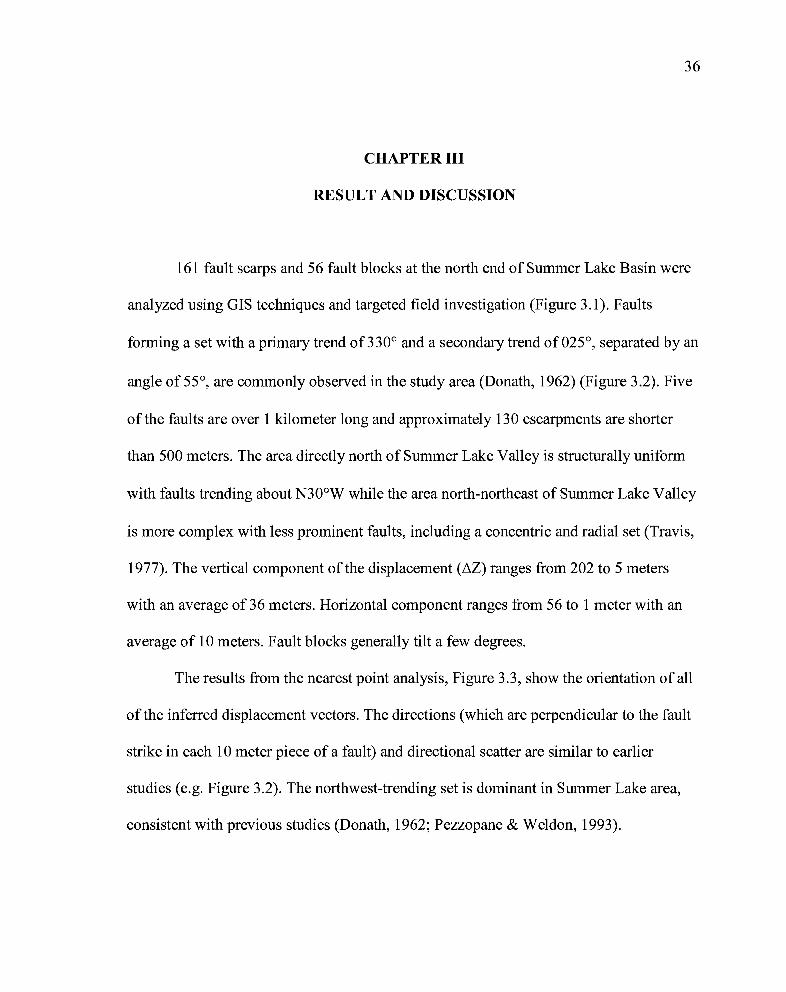
161 fault scarps and 56 fault blocks at the north end of Summer Lake Basin were

analyzed using GIS techniques and targeted field investigation (Figure 3.1). Faults

forming a set with a primary trend of 330° and a secondary trend of 025°, separated by an

angle of 55°, are commonly observed in the study area (Donath, 1962) (Figure 3.2). Five

of the faults are over 1 kilometer long and approximately 130 escarpments are shorter

than 500 meters. The area directly north of Summer Lake Valley is structurally uniform

with faults trending about N300W while the area north-northeast of Summer Lake Valley

is more complex with less prominent faults, including a concentric and radial set (Travis,

1977). The vertical component of the displacement (~Z) ranges from 202 to 5 meters

with an average of 36 meters. Horizontal component ranges from 56 to 1 meter with an

average of 10 meters. Fault blocks generally tilt a few degrees.

The results from the nearest point analysis, Figure 3.3, show the orientation of all

of the inferred displacement vectors. The directions (which are perpendicular to the fault

strike in each 10 meter piece of a fault) and directional scatter are similar to earlier

studies (e.g. Figure 3.2). The northwest-trending set is dominant in Summer Lake area,

consistent with previous studies (Donath, 1962; Pezzopane & Weldon, 1993).

37

Figure 3.1. 161 fault scarps (upper) and 56 fault blocks (lower) at the north end ofSummer Lake Basin.

38

w E

Figure 3.2. 625 faults and fault segments plotted at 1° intervals. Radius ofdiagramequals 18 faults or fault segments. A conjugate fault set ofprimary trending 330° andsecondary trending 025°. (from Donath, 1962)

Figure 3.3. Rose diagram from near point analysis illustrates ENE-WSW azimuthaldistribution ofthe offset vectors. Each bin is proportional to the number of fault scarps.Strike approximately normal to offset vector.

39

Due to the limitation to access in some sections of the study area, the

representative orientation of faults were measured in four locations to determine an

average fault dip and slip direction to be assigned to faults for which we cannot directly

observe the dip or slip direction (Figure 3.4 and Table 1). The orientation of

representative faults show steeply dips, striae are sub-vertical and very close to pure

normal so we assume that the average slip direction is down dip. Since the representative

faults dip both east and west (Figure 3.5), the average will be very steep (87 degrees,

Figure 3.6) which may improper for a typical normal fault we found elsewhere in the

nature. So we would abandon this average value and will not take it into account in our

calculation. We used the average dip of all of the faults, ~74 degrees, instead of the

average dip of the average fault which is shown on the stereonet.

The orientation of representative faults and associated striae can be divided into 3

domains with dominate striking ofNNW-SSE, east dipping (domain 1), NNE-SSW, west

dipping (domain 3) and conjugate mixed set with opposite dips of domain 1 and 3 with

the opposite dips and several EW planes (domain 2) (Figure 3.6 and 3.7). The NNW

faults (domain 1) are right oblique; 2 slickenlines are left oblique and 4 are right oblique

but all are within 15 degrees of pure dip slip. The domain 3 shows NNE west dipping

faults as mainly right slip (i.e., a mixture of slightly right and slightly left, very close to

pure normal). The mixed set, domain 2, is similarly mixed in their oblique components,

so the bottom line is that there really is no strong sense of oblique slip seen in these data

and it supports essentially pure normal no matter what the fault orientation.

40

Table 1. Orientation of a representative faults and slickenlines measured from the field.

Location Strike/dip Rake

S83°W 8l oW nowSlOoW 800 W 82°SW

Lac. #1 N28°W 89°NE 84°SE

ION 0684262 EW nos 89°E

4764166S53°E 76°S 900E

N400W 63°N 900S

S32°W 62°W -

N18°W 87°NE 8l oSE

SlOoW 59°NW 82°SW

Lac. #2 S28°W 54°NW 68°NW

ION 0689499 SlloE 80 0 W 6l oSE

4769354 N29°W 8loNE 76°SE

N200W 82°E 74°SE

S43°E 82°S 78°SE

N58°W 8loNE -

Lac. #3

ION 0696718N8°E 500S

-4768672

N44°E 8l oSE 55°SW

Lac. #4 N73°E 76°SE 74°E

ION 0696723 N37°W 8l ONE nON

4768656 N700E 75°E 74°W

N33°E 70 0 E 59°S

41

Figure 3.4. Location of representative orientation of faults and slickenlines collected1:i-om the field. The numbers refer to locations fi:om Table 1.

Figure 3.5. The outcrop at location#2 showing faults and associate striae. Faults showinga variety of dips.

42

.j-;.• ••

••

Figure 3.6. Stereonets of representative faults and slickenlines in study area.(Upper) Poles to fault planes show steep dips regardless of the strike; we used theaverage dip of all of the faults for our best estimate. Dashed line is the averageorientation; because faults dip both east and west, the dip is not meaningful, but thestrike, ~NI5W, matches our minimum extension direction.(Lower) Slickenlines on fault planes are steep and suggest generally dip slip motionregardless of the fault strike. Mean lineation direction is 82° S24°W.

43

..<.---------t---- -. --........;(' ~ "-

:(\ I ~

//~" '"~, \

--........_----~

I Domain 1 I I Domain 2

I Domain 3 I

Figure 3.7. Stereonets of faults and slickenlines collected in the field, broken into 3distinct groups: NNW-SSE, east dipping (domain 1), NNE-SSW, west dipping (domain3) and conjugate mixed set that included faults with similar trends as domains 1 and 3,but opposite dips, and several EW planes (domain 2).

44

Extension Direction

As mentioned earlier in Chapter 1, the top-bottom fault traces were broken into

10-meter segments and reference coordinates were assigned to measure the directions and

distances in the nearest point analysis (Figure 1.10). The frequencies of offset and

extension distribution were plotted azimuthally to see how extension varies with

direction. The distribution of the offsets on individual fault was varied by fault geometry

regardless of its size. The directional variations of the offset due to faults' geometries are

shown in figure 3.8. The straight faults produce little variability (e.g. fault 23) whereas

more variable yield a range in both directions (Rose diagram) and offsets (histogram).

The straight faults (fault 23) show the dominate NNW trend, bent faults (fault 22) show

the two major trends and curved fault provides normal distribution. The peaks of these

offset vectors either on histogram or Rose diagram will response to the stretching

direction on each fault, combining these directions for all faults will resolve extension

direction.

The offsets of every single fault were plotted azimuthally to see the extension

direction of the area (Figure 3.9). Azimuthal frequency distribution is bimodal, reflecting

the approximately equal number of east and west dipping faults. The fact that the

variation changes systematically with azimuth, suggests a single distribution offaults in

the study area which probably developed at the same time and their movements were

contemporaneous. The maximum extensional direction is ~ N75°E. The fact that

extension diminishes to zero at ~N 15°W suggests that the minimum horizontal strain axis

(and maximum horizontal stress axis) is oriented in this direction. Since there is no

~ ~

0.. riO·o cS '"':-" (l)::l W~ .(D"QO

-+::­Vl

///

-'.,

"" "-

N

§§

[CDooo

C>

8

Offset..go,

N

8o

0-1010-2020-3030-4040-5050-6060-7070-8080-90

90-100100-110110-120120-130130-140140-150150-160160-170170-180180-190

190-200~200-210210-220220-230230-240240-250250-260260-270270-280280-290290-300300-310310-320320-330330-340340-350

350-360,L- ----'

~

2S'

~C> ...,o 0o 08 8

[~;;

...~.;J

Offsetw .t> 0'o 0 0

§ § §Noooo

oo8

0-1010-2020-3030-4040-5050-6060-7070-8080-90

90-100100-110110-120120-130130-140140-150150-160160-170170-180180-190190-200200-210210-220

220-230E230-240 l!!!I!!!!iiiiii••••••••240-250250-260260-270270-280280-290290-300300-310310-320320-330330-340340-350350-360 [ [

~~.

S'

.......

C/)

6:2C/)

8'....,S"0..

<"0.:ce:.Et-c

-:luC1l~N

3c.......ue:.<e;a"0"::lo....,.......uC1lo6f5C1l.......

C/J.......~

<fO"g-~c

.......~5-C/)

C/)

uo:2C/)

?o0..o35"~C1l

~C.......

.......~::l0..~::l0..UC1l::l.......

46

extension in the ~N15°W direction (Figure 3.8), vertical thinning must equal the

extension in the ~ N75°E direction in order to preserve mass. Therefore, this area is

experiencing plane strain. This estimated extension direction is supported by orientation

of faults collected fi'om the field. Representative faults average N15°W direction (Figure

3.5) and ifthe plane strain assumption is applied, there will be no extension along this

direction.

200000

I 150000

ill~~ 100000(5I-

Azimuth

Figure 3.9. Azimuthal distribution of the offset suggesting faults in study area developedat the same time and the movement were contemporaneous

Magnitude of Extension

The top and bottom boundaries of fault scarps were divided into IO-meter

segments where the reference points were generated along the tracing lines. The

coordinates of the reference point on each segment and vertical component displacement

47

(i1Z) on top-bottom of each fault were used to calculate the offsets and extension by

using the trigonometric relationships

offset = i1Z / Sin(8)

extension = i1Z / Tan(8)

where 8 is average dip obtained from the field (74.38 degrees in this study).

As mentioned in Equation 2 the original area Ao is calculated by measuring the expanded

area Ae of the representative area at the north end of Summer Lake basin using GIS and

subtracting the area occupied by faults and tilted fault blocks Aa• The length of the major

axis has been resolved.

The magnitude of extension is estimated 1.5 to 5.5 percent along the maximum

extension direction. Estimated areas added by extension and calculated from equation 1

in Chapter I, are shown in Table 2. The amount of extension is estimated assuming both

planar faults to depth and steep surface faults curving into listric detachment fault,

providing the minimum and maximum possible extension. The common occurrence of

tilted fault surface blocks strongly suggests that faults have curved surfaces rather than

planar surfaces at depth (Travis, 1977). The geometry of the main fault in detachment­

rooted normal faults can create a void, which is often filled by secondary or antithetic

faults. The roll-over structure is specific to a listric fault geometry, while the planar faults

provided many antithetic faults (Faure & Chermette, 1989). An array ofparallel normal

faults associated with minor antithetic faults are commonly observed on the outcrop in

the field, suggest that major faults in the study area are listric.

48

In addition, the average dip measured in the field was much steeper than what

most normal faults are believed to have, I also made the calculations assuming 60°

degrees and it doubles the amount of extension one would calculate (Table 2).

Tilted Fault Blocks

The blocks between the faults in the study area are nearly flat with the steepest

dipping approximately 5 degrees (Travis, 1977). Visually, it appears that the tilt ofblocks

can be obtained from surface slopes. To make sure that the slope on the surface of the

blocks is the dip of beds in the block, the tilt ofblocks was measured from the surface

slope and compared to the strike and dip determined the from the basalt tracing method

described inChapter 2 (Table 3). Surface slopes generally correspond to the tilt of beds in

most places but a few are different. The error may be caused by the discontinuity of

bedding planes on fault scraps that make the tracing lines hard to follow. However,

results from surface slopes are reasonable and comparable, so we use them where we do

not have tilts from the volcanic layering within blocks.

The estimated extension acquired from tilted fault blocks in the study area is

consistent with other studies where faults with a dip of 5° to 10° have extension

equivalent to about 10% where as faults with dips more than 45° have extension

equivalent to more than 100% (Proffett, 1977; Anderson, 1971; Wright & Troxel, 1973).

Herein for an average few degrees in the study area indicates 1.5 to 5.5 percent extension.

Many studies indicate extension of about 20-30% for entire Great Basin region using a

technique that relates dips of bed and extension on the tilted fault blocks (Morton &

49

Black, 1975) or Proffett (1977) using other data obtained the result that amount of

extension in Basin and Range Province varies from area to area. Since our study does not

include the major range forming faults (i.e. Winter Rim, Diablo Rim and Abert Rim) we

are only seeing a fraction of the total deformation.

Table 2. Estimated strain of the study area.

Initial dip = 74.38° Initial dip = 60°

Ae [m2] 555,369,807.88 555,369,807.88

Planar fault

Aa [m2] 7,039,871.59 14,537,708.04

Ao [m2] 548,329,936.29 540,832,099.84

a-axis 13,211.31 13,120.68

b-axis 13,380.93 13,473.37

Percent change 101.28 102.69

Listric fault

Aa [m2] 26,145,643.18 29,075,416.08

Ao [m2] 529,224,164.70 526,294,391.80

a-aXIS 12,979.11 12,943.13

b-axis 13,620.33 13,658.18

Percent change 104.94 105.52

Table 3. Comparing amount of tilt obtained from basalt bed and surface slope.

Measured tiltBlock ill Bedding

from bedding plane from surface slope

2 b2 1 3.350509 2.577035

b2 2 4.031433 2.577035

4 b4l 4.259658 4.762176

b42 3.569953 4.762176

b43 7.774043 4.762176

5 b5 1 5.285455 4.91479

b5 2 9.288711 4.91479

6 b6 1 2.556545 4.729436

b6 2 5.015185 4.729436

b6 3 15.399195 4.729436

7 b7 1 5.053379 3.713142

b7 2 1.860022 3.713142

b7 3 0.553182 3.713142

b7 4 2.759043 3.713142

b7 5 0.955491 3.713142

9 b9 2.953646 1.787224

10 b10 1.101431 2.691441

11 b11 2.682819 2.248956

44 b44 0.386276 0.88942

47 b47 2.280503 2.585157

48 b48 0.440043 1.71695

50

51

As discussed above in the Introduction, we initially intended to explicitly include

block tilt in our calculations, so we would not have to know the geometry of the faults at

depth. However, we found that on average the blocks did not tilt in the extension

direction, which makes the calculation of their contribution to extension much more

difficult. Thus we decided to simply bracket the extension by assuming the greatest and

least possible dips at depth. The fact that the tilt is not in the same direction of its

extension, probably means that the dip oflow angle faults underneath was not controlled

by extension, and thus may have followed pre-existing weakness or regional layering in

the volcanic rocks. Result fi'om this study showed blocks tilt on average 60° from the

maximum extension direction (Figure 3.10) indicates that the fault pattern in the region

was probably controlled by reactivation of basement structure which is approximately

150,-----------------------------------,

125

~ 1000..Q

~ 75'iii<I>

~50

25

Aspect

Figure 3.10. Aspect of tilted fault blocks. Blocks tilt on average of 60° fi'om themaximum extension direction (075° and 255°) suggested that the detachment surface isprobably controlled by reactivation of basement structure or the pre-existing dip oflayering underneath.

52

We decided not to explicitly use the dips ofthe blocks because we decided to use

the fault displacement to get at extension if the faults are listric (Figure 1.88). However

the tilt of the blocks, and especially the fact that certain regions have consistently dipping

blocks suggests that the faults root into some sort of detachment, and thus the approach

we use to get the extension that assume a detachment is reasonable. Furthermore, we can

fit the strain ellipse to the area added Aa to get the real magnitude and direction of

extension (Appendix A). Results indicate total extension of 5.14% in an azimuth of

73.35°, almost identical to the result from GIS teclmique (Figure 3.11 and 3.12).

2500000-.----------------------------------,

_ADDED AREA [m2]

2000000

-g 1500000'0'0roro

~ 1000000

Approx areas

Azirruth

Figure 3.11. Estimated extension using our added area approach compared with anellipse with the same area. (Red) Added area assuming a perfect strain ellipse. (Blue)Area added from this study.

53

0.5

-0 5

-1

-1.5

...+.,

\'t'.

-1 -0.5 0.5

.I

1.5

x 10·

Figure 3.12. Strain ellipse fitting using least squares method. Major axis has a length of1.0514 and minor axis is rotated 16.6451° West ofNOlth indicating extension 01'5.14%in the direction ofN73°E. The extension data from the GIS technique (blue) very closelymatches the shape of the fit ellipse (red).

This new technique does not require one to collect information across the whole

region to estimate deformation. Instead, we can pick representative areas that characterize

the deformation in a broad area. This method has the advantage for studying areas that

are difficult to access and collect data. For instance, Donath (1962) could not determine

dips for about 85% of the faults by using air photograph and observations in the field.

This new technique provides a methodology to obtain the orientation data and make a

robust estimate of the strain. Undoubtedly, this methodology can be applied to any parts

of the world especially in other part of Basin and Range Province that undergo uniform

deformation, even for some complex regions where we cannot collect the orientation of

fault easily such as in the east portion of study area.

54

APPENDIX A

FITTING AN ELLIPSE TO DETERMINE ADDED AREA

Approximating Radii

In order to detennine the size and orientation of a strain ellipse that best matches

the azimuthal variation in extension detennined from my GIS analysis, I used an ellipse-

fitting program written by fellow Graduate Student Sequoia Alba, Because the program

requires a list of coordinates (points in x, y), I found values for the radius of the ellipse

centered between the two outside angles by approximating the area of a 10 degree section

of a circle. I then found the radius of that circle for each added area using:

r =e

where Ae is the added area in a 10 degree section, Ae = total expanded area -total added

area (Figure A).The added radius is detennined by subtracting the radius ofthe inscribed

circle de = re - re. I then used the angles and radiuses to get a list of x andy coordinates to

plug into the ellipse fitting program.

55

ial

Figure A. Original area in circle Ao and extended area in ellipse A('. The different areabetween circle and ellipse is "area added", Ail'

Ellipse Fitting

The ellipse fitting program uses a least squares method to find the equation for the

ellipse described by the second order polynomial:

Ax 2 + Bxy+Cy 2 +Dx+Ey+F =0

It then finds the "bit" of the ellipse and subtracts it to get the new equation ofthe untitled

ellipse: A' x 2 + C' y2 + F = 0 . The major and minor axes are inferred ii-om the

coefficients of the polynomial.

Approximated Areas

To get the list of approximated areas I used the parametric equations for an ellipse

rotated counter clockwise by ¢J:

x = a cos( () )cos( ¢ ) - b sin( () )sin( ¢J ) y = a cos( () )sin( ¢ ) + b sin( () )cos( ¢J )

and integrated the polar equation for the area over 10 degree increments clock-wise from

. h 2 2 2wIt r = x + Y .

The resulting comparison are shown in Chapter 3 (figure 3.11 and 3.12).

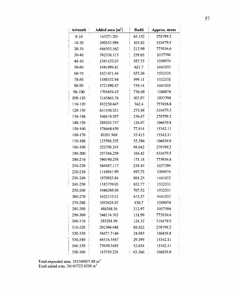
APPENDIXB

APPROXIMATED AREAS FROM FITTING ELLIPSE

56

57

Azimuth Added area [m2l Radii Approx. areas

0-10 143271.201 63.152 278799.2

10-20 240553.986 105.82 510479.5

20-30 486303.562 212.99 773936.6

30-40 592530.515 259.05 1037394

40-50 1361422.03 587.75 1269074

50-60 1441899.61 621.7 1441033

60-70 1521671.44 655.26 1532531

70-80 1388332.84 599.11 1532531

80-90 1721898.87 739.14 1441033

90-100 1701654.42 730.69 1269074

100-110 1163665.76 503.97 1037394

110-120 832258.647 362.4 773936.6

120-130 631450.321 275.88 510479.5

130-140 540418.387 236.47 278799.2

140-150 288203.757 126.67 106839.8

150-160 176664.459 77.814 15342.11

160-170 80201.968 35.415 15342.11

170-180 125598.525 55.386 106839.8

180-190 222798.243 98.042 278799.2

190-200 237366.259 104.42 510479.5

200-210 390190.258 171.18 773936.6

210-220 544987.117 238.45 1037394

220-230 1148941.99 497.72 1269074

230-240 1870925.84 801.25 1441033

240-250 1515759.05 652.77 1532531

250-260 1646268.96 707.52 1532531

260-270 1422152.01 613.37 1441033

270-280 1052624.87 456.7 1269074

280-290 486268.56 212.97 1037394

290-300 346174.703 151.99 773936.6

300-310 283281.99 124.52 510479.5

310-320 201304.448 88.622 278799.2

320-330 54471.7146 24.083 106839.8

330-340 66516.5467 29.389 15342.11

340-350 73930.3485 32.654 15342.11

350-360 143759.224 63.366 106839.8

Total expanded area: 555369807.88 m2

Total added area: 26145722.4298 m2

58

REFERENCES

Allison, 1. S. (1949). Fault pattern of south-central Oregon [Abstract]. Geological SocietyofAmerica Bulletin, 60, 1935.

Anderson R. E. (1971). Thin skin distension in Tertiary rocks of southeastern Nevada.Geological Society 0.[America Bulletin, 82, 43-58.

Badger, T. c., & Watters R. J. (2004). Gigantic seismogenic landslides of Summer Lakebasin, south-central Oregon. Geological Society ofAmerica Bulletin, 116, 687­697.

Clifton, A. E., Schlische, R. W., Withjack, M. 0., & Ackermann, R. V. (2000). Influenceof rift obliquity on fault-population systematics: results ofexperimental claymodels. Journal ofStructural Geology, 22, 1491-1509.

Cloos, E. (1955). Experimental analysis of fracture patterns. Geological Society ofAmerica Bulletin, 66, 241-256.

Cloos, H. (1936). Einfuhrung in die Geologie. Berlin: Borntraeger.

Crider, J. G., & Pollard, D. D. (1998). Fault linkage: three-dimensional mechanicalinteraction between echelon normal faults. Journal ofGeophysical Research, 103,24,373-24,391.

Crider, J.G. (2001). Oblique slip and the geometry of normal-fault linkage: mechanicsand a case study from the Basin and Range in Oregon. Journal ofStructuralGeology, 23, 1997-2009.

Donath, F.A. (1962). Analysis of Basin and Range structure. Geological Society ofAmerica Bulletin, 71, 1-15.

Donath, F.A., & Kuo, J.T. (1962). Seismic refraction study of block faulting, South­Central Oregon. Geological Society ofAmerica Bulletin, 73, 429-434.

ESRI (2007). Arc GIS 9.2 Help: Near (Analysis). Retrieved February 6,2009, fromhttp://webhelp.esri.com/arcgisdesktop/9.2/index.cfm?id=1111 &pid= 11 07&topicname=Near_(Analysis)

59

Faure, l L., & Chermette, J. C. (1989). Deformation oftilted blocks, consequences onblock geometry and extension measurements. Bulletin de la Societe Geologiquede France, 3, 461-476.

Hamilton, W., & Myers, W. B. (1966). Cenozoic tectonics ofthe western United States.Reviews ofGeophysics, 4,509-549.

Kautz, S.A., & Sclater, lG. (1988). Internal deformation in clay models of extension byblock faulting. Tectonics, 7, 823-832.

Lawrence, R D. (1976). Strike-slip faulting terminates the Basin and Range province inOregon. Geological Society ofAmerica Bulletin, 87, 846-850.

McClay, K. R, & Ellis, P. G. (1987). Analogue models of extensional fault geometries.Geological Society, London, Special Publications, 28, 109-125.

Morton, W.H. & Black, R (1975). Crustal attenuation in Afar. In: Pilger, A. & RosIer, A.(Eds.), Afar depression ofEthiopia, Inter-Union Commission on GeodynamicsScientific Report No. 14 (pp. 55-65). Stuttgart: Schweizerbart.

Pease, R W. (1969). Normal faulting and lateral shear in northeastern California.Geological Society ofAmerica Bulletin, 80, 715-720.

Pezzopane, S.K., & Weldon II, Rl (1993). Tectonic role of active faulting in centralOregon. Tectonics, 12, 1140-1169.

Piper, A. M., Robinson, T. W., & Park, C.F., Jr. (1939). Geology and ground-waterresources of the Harney basin, Oregon. Us. Geological Survey Water-SupplyPaper, 841. 189.

Proffett, l M., Jr. (1977). Cenozoic geology of the Yerington district, Nevada, andimplications for the nature and origin ofbasin and range faulting. GeologicalSociety ofAmerica Bulletin, 88, 247-266.

Reches, Z. (1978). Analysis of faulting in three-dimension strain field. Tectonophysics,47, 109-129.

Stewart, lH. (1980). Regional tilt patterns oflate Cenozoic Basin-Range fault blocks,western United States. Geological Society ofAmerica Bulletin, 91, 460-464.

Travis, P. L., Jr. (1977). Geology ofthe area near the north end ofSummer Lake, LakeCounty, Oregon, Unpublished master's thesis, University of Oregon, Eugene,Oregon.

60

Weldon, R. 1. II., Fletcher, D. K, Weldon, E. M., Scharer, K M., & McCrory, P.A(2002). An update ofQuaternary faults ofcentral and eastern Oregon [CD­ROM]. (U.S. Geological Survey Open-File Report 02-301).

Wright, L. A, & Troxel, B. W. (1973). Shallow-fault interpretation ofBasin and Rangestructure, south-western Great Basin. in Dejong, R., and Scholten, R. (Eds.),Gravity and tectonics (pp. 397-407). Amsterdam: Elsevier Scientific PublishingCompany.

Zoback, M. L., Anderson, R. E., and Thompson, G. A (1981). Cenozoic evolution ofthestate of stress and style of tectonism ofthe Basin and Range Province ofthewestern United States: Phil. Trans. Roy. Soc. London A, v. 300,407-434.