exterior insulation systems containing vacuum insulation...

ORNL/TM-2012/276

Exterior Insulation Systems Containing Vacuum Insulation Panels Tested Using a Heat Flux Meter Apparatus

August 2012

Prepared by Kenneth Childs Therese Stovall Kaushik Biswas Jerry Atchley

ii

DOCUMENT AVAILABILITY

Reports produced after January 1, 1996, are generally available free via the U.S. Department of Energy (DOE) Information Bridge.

Web site http://www.osti.gov/bridge

Reports produced before January 1, 1996, may be purchased by members of the public from the following source.

National Technical Information Service 5285 Port Royal Road Springfield, VA 22161 Telephone 703-605-6000 (1-800-553-6847) TDD 703-487-4639 Fax 703-605-6900 E-mail [email protected] Web site http://www.ntis.gov/support/ordernowabout.htm Reports are available to DOE employees, DOE contractors, Energy Technology Data Exchange (ETDE) representatives, and International Nuclear Information System (INIS) representatives from the following source.

Office of Scientific and Technical Information P.O. Box 62 Oak Ridge, TN 37831 Telephone 865-576-8401 Fax 865-576-5728 E-mail [email protected] Web site http://www.osti.gov/contact.html

This report was prepared as an account of work sponsored by an agency of the United States Government. Neither the United States Government nor any agency thereof, nor any of their employees, makes any warranty, express or implied, or assumes any legal liability or responsibility for the accuracy, completeness, or usefulness of any information, apparatus, product, or process disclosed, or represents that its use would not infringe privately owned rights. Reference herein to any specific commercial product, process, or service by trade name, trademark, manufacturer, or otherwise, does not necessarily constitute or imply its endorsement, recommendation, or favoring by the United States Government or any agency thereof. The views and opinions of authors expressed herein do not necessarily state or reflect those of the United States Government or any agency thereof.

iv

ORNL/TM-2012/276

Energy and Transportation Science Division

EXTERIOR INSULATION SYSTEMS CONTAINING VACUUM INSULATION PANELS TESTED USING A HEAT FLUX METER

APPARATUS

Kenneth Childs Therese Stovall Kaushik Biswas

Jerry Atchley

Date Published: August, 2012

Prepared by OAK RIDGE NATIONAL LABORATORY

Oak Ridge, Tennessee 37831-6283 managed by

UT-BATTELLE, LLC for the

U.S. DEPARTMENT OF ENERGY under contract DE-AC05-00OR227

vi

Table of Contents

Abstract ....................................................................................................................................................... 1

1. Introduction ............................................................................................................................................. 2

2. Measurement Methodology .................................................................................................................... 3

3. Description of Specimens Tested ............................................................................................................. 4

4. Test Data .................................................................................................................................................. 6

5. Mapping Heat Flux Transducer Readings to Full VIP Assemblies .......................................................... 21

6. Extraction of VIP Thermal Properties from Test Data ............................................................................ 27

7. Numerical Modeling of VIPs .................................................................................................................. 37

8. Summary and Conclusions ..................................................................................................................... 40

Appendix A – Heat Flux Meter Apparatus Application for Nonhomogeneous Low Thermal Conductivity Specimens .................................................................................................................................................. 41

A.1 Heat Flux Transducer Calibration .................................................................................................... 41

A.2 Uncertainty Evaluation .................................................................................................................... 47

A.3 Test Duration ................................................................................................................................... 48

A.4 Repeatability .................................................................................................................................... 49

A.4.1 Design Option 5, Single-‐Piece Test Specimen with One Large VIP ........................................... 49

A.4.2 Design Option 1, Three-‐Piece Test Specimen with Two Small and One Large VIPs ................. 53

Appendix B – List of all Heat Flux Meter Apparatus Tests ......................................................................... 59

References ................................................................................................................................................. 60

Abstract A proposed wall system that will provide a high thermal resistance in a relatively thin profile incorporates vacuum insulation panels (VIP) enclosed within closed-‐cell insulating foam. In addition to providing some additional thermal resistance, the foam protects the vacuum panels during construction and provides a surface appropriate for an adhesive joint on both sides of the foam-‐VIP unit. Multiple configurations of the composite structure were considered and experimental measurements were sought to provide more information in the final selection. Small sub-‐sections of each candidate arrangement were prepared and tested in a special-‐purpose heat flux meter apparatus. Those measurements are described here, along with additional modeling efforts based on these smaller-‐scale measurements. The focus of the tests reported here is to investigate the impact of vacuum panel size, the type of foam used to encase the vacuum panels, the thickness and shape of the foam sections between panels, and possible adhesive effects. A new procedure was developed to map the heat flux meter measurement results onto full-‐scale wall designs to predict the system thermal performance. Several potential arrangements of the foam-‐VIP unit were also evaluated using a finite-‐difference methodology. The report also evaluates procedures for testing VIPs in a heat flux meter apparatus, and makes some recommendations.

2

1. Introduction

Dow Corning Corporation, a joint venture of Dow Chemical Company and Corning Inc., is working with the U.S. Department of Energy and Dryvit Systems, Inc. to develop a wall system that will provide a high thermal resistance in a relatively thin profile. The proposed wall system incorporates vacuum insulation panels (VIP) enclosed within closed-‐cell insulating foam. In addition to providing some additional thermal resistance, the foam serves to protect the vacuum panels during construction and to provide a surface appropriate for an adhesive joint on both sides of the foam-‐VIP unit. Multiple configurations of the composite structure were considered and experimental measurements were sought to provide more information in the final selection.

The Oak Ridge National Laboratory is contributing to the process by measuring the thermal transmission of complete wall sections in a guarded hot box and in a natural exposure test facility in Charleston, SC. These tests are rather large in scale and cost, so it is not practical to perform separate wall-‐scale tests for each of the foam-‐VIP arrangements under consideration. Therefore, before building test wall sections, smaller sub-‐sections of each candidate arrangement were prepared and tested in a special-‐purpose heat flux meter apparatus. Those measurements are described here, along with additional modeling efforts based upon these smaller-‐scale measurements. The focus of the tests reported here is to investigate the impact of vacuum panel size, the type of foam used to encase the vacuum panels, the thickness and shape of the foam sections between panels, and possible adhesive effects. A new procedure was developed to map the heat flux meter measurement results onto full-‐scale wall designs to predict the system thermal performance. Several potential arrangements of the foam-‐VIP unit were also evaluated using a finite-‐difference methodology. All of the vacuum panels were prepared using commercial equipment. The barrier material is a laminate of three metallized polyester films and a linear, low-‐density polyethylene heat-‐seal layer. The filler material is a fine powdered form of silica with additives to reduce radiative heat transfer.

The report also evaluates procedures for testing VIPs in a heat flux meter apparatus, and makes some recommendations. Note that the effective R-‐value of a single VIP panel cannot be clearly defined independent of an assembly. Because the VIP is non-‐homogenous, with significant edge heat flow, the R-‐value will vary according to the boundary conditions surrounding the surfaces.

3

2. Measurement Methodology The heat flux meter apparatus is a secondary measurement method, often used to evaluate the thermal conductivity of homogenous materials. The typical construction and use are described in ASTM C518 [ASTM 2010]. The two plates, shown in Figure 1, are carefully controlled at fixed temperatures. As the heat flows from the hot plate and through the test specimen into the cold plate, a small temperature difference across the transducers generates an electrical signal that is proportional to the heat flux through the transducer. For homogenous specimens with uniform plate temperatures, the heat flux is unidirectional and can therefore be used with Fourier’s Law to calculate the thermal conductivity of the material.

Figure 1 Conceptual cross section of a heat flux meter apparatus

Most heat flux meter apparatus use a single transducer on each of the temperature-‐controlled plates. A special-‐purpose apparatus has been designed to facilitate the characterization of non-‐homogenous specimens. This apparatus has an array of transducers on both the top and bottom plates, so that non-‐uniform heat flux patterns can be measured. The design of this array is shown on Figure 2. The test produces a map of heat transfer over this collection of thirty (15 top and 15 bottom) 7.5 x 7.5 cm (3 x 3 in.) transducers. Even with this extensive measurement scheme, it is typically necessary to merge the test measurements with a mathematical model to fully characterize complex specimens. This apparatus has previously been used to examine vacuum insulation panels as a part of a refrigerator design project. [Wilkes et al, 1997; Wilkes et al, 1999; Stovall and Brzezinski, 2002]

A non-‐standard calibration method, similar to that described in ASTM C1667, was used for this project to more accurately measure very small heat flux values. [ASTM 2009] The calibration process, along with other test practice details, is described in Appendix A. Using this calibration process, the heat flux values reported here have an extended combined uncertainty between 5 and 10% at a 95% confidence level, with the greater uncertainty corresponding to the lower heat flux values found over the center of a vacuum insulation panel. [Taylor and Kuyatt, 1994]

4

Figure 2 Heat flux transducer numbering scheme -‐ 1 (back of heat flux meter), 5 (left edge), 11 (right edge), 15 (front)

3. Description of Specimens Tested

In order to use vacuum insulation panels in a building, it is necessary to protect them from puncture and abrasion during the construction process. In the proposed designs, that is accomplished by encasing the vacuum panels within closed cell foam insulation. Within this general design framework, there are a large number of possible permutations with regard to: the arrangement of panel seams relative to joints where panels are adjacent to each other, the type of foam insulation, the thickness of the foam separation between vacuum insulation panels, and other possible protective materials.

Ten special purpose test specimens were prepared to place these variations within the monitored area of the heat flux meter apparatus. Figure 3 demonstrates how these test specimens are representative of panel intersections within a full wall. The joints between VIPs in the test specimens were located along the lines of central transducers. All of the assemblies cover an area slightly less than 610 x 610 mm (24 x 24 in.) and consist of a layer containing 2.5 cm (1in.)-‐thick VIPs sandwiched between layers of rigid foam insulation, either expanded polystyrene (EPS) or extruded polystyrene (XPS). The assemblies differ in (1) the number and size of VIPs they contain (one large panel, two half panels or one half panel with two quarter panels), (2) the type and thickness of the rigid foam insulation layers and (3) the material adjacent to the edges of the VIPs. An example of an assembly construction is illustrated in the exploded view of Design Option 1 shown in Figure 4. A summary of the key features of the VIPs tested is given in Table 1. Some internal details of Design Options 11 and 12 could not be determined by visual examination of the assemblies.

5

Figure 3 Test specimen represents joints between panels on a full wall

Table 1 Test specimen construction details.

Design Option No. VIPs

Material Surrounding VIPs Layers (from top to bottom) Assembly Edges Between VIPS 1 2 3 4

1 3 0.5” XPS 1” XPS 1” XPS 1” VIP 1” EPS — 2 3 0.5” XPS 1” XPS 1” EPS 0.5” XPS 1” VIP 0.5” EPS 3 3 0.5” XPS 1” XPS 1” EPS 0.5” XPS 1” VIP 0.5” XPS 4 3 0.04” PVCa 0.08” PVCa 1” EPS 1” VIP 1” EPS — 5 1 0.5” XPS 1” XPS 1” EPS 1” VIP 1” XPS — 6 3 0.5” XPS 1” XPS 1” XPS 1” VIP 1” XPS — 8 3 0.5” EPS 1” XPS 1” EPS 1” VIP 1” EPS —

10 2 0.5” XPS

Butt joint, edge to edge (not flap to

flap)

1” XPS 1” VIP 1” XPS —

11 3 Silicone sealant + Gap

Butt joint, edge to edge (not flap to

flap)

1” EPS 1” VIP 1” EPS —

12 3 ? ? 1” EPS 1” VIP 1” XPS — a PVC was approximately 50 mm (2 in.) high, covering the side of the VIP and the side of the bottom foam, so that it touched the bottom plate of the apparatus but not the top plate

6

In addition to the 10 VIP assemblies, tests were also performed on two bare VIPs that were approximately 23.5” square (59.6 cm). The thermal conductivity of EPS and XPS foam boards similar to those used in the assemblies was measured.

Figure 4 Exploded view of Design Option 1

4. Test Data Each of the assemblies contains EPS insulation board, XPS insulation board, or a combination of both. Since the conductivity of these materials influences the performance of the assemblies, a series of heat flux meter apparatus tests were performed to determine the thermal conductivity of both EPS and XPS as a function of temperature. The temperature-‐dependent thermal conductivity of EPS and XPS from these measurements is given by Eq. 1 and 2, respectively, and shown in Figure 5.1

𝑘 = 3.4020×10!! + 1.4591×10!!𝑇 , Eq. 1

𝑘 = 2.5638×10!! + 1.1688×10!!𝑇 Eq. 2

where T = temperature, °C K = thermal conductivity, W/m-‐K.

1 The VIP assemblies used in the full-‐scale Rotatable Guarded Hot Box (RGHB) wall assembly used a different EPS than that used in the assemblies discussed here. This second EPS was tested at a single temperature and found to have a slightly lower thermal conductivity.

7

In the series of the tests performed on the ten VIP assemblies and two large individual VIPs the bottom plate temperature is set to 35°C and the top plate temperature is set to 12.78°C. Some of the specimens were measured multiple times, as shown in the list of tests in Appendix B. The following pages give the measured fluxes from a representative test for each of the specimens. The top figure on each page gives the measured flux (W/m2) for each heat flux transducer (transducer) location. The top number for each location is the flux on the upper surface, and the bottom number is the flux on the lower surface. Note that HFT 12 on the bottom plate is inoperable, and HFT 11on the upper plate operates only intermittently. To aid in interpreting the fluxes, the location of each VIP in the assembly is also outlined on the figure. The white space represents the material surrounding the VIP(s). At the bottom of each page are two plots of the heat fluxes along the two centerlines of the transducer array. Uncertainty bounds of 7.5% are shown on these plots.

Figure 5 Foam board thermal conductivity

Look at these results for Design Option 1 in Figure 6 and Figure 7. As you travel across the x axis from left to right, you see the flux is slightly greater near the edges, but the greatest heat flux occurs at the center of the specimen, where x and y are both equal to zero. This is the transducer location with the maximum area of foam insulation and the minimum amount of VIP coverage. As you travel along the y-‐axis in the right half of Figure 7, notice the heat flux drops significantly as the y-‐value increases, which corresponds to the positive y-‐values, or the top half of Figure 6, where the transducer is located over the center of a VIP and farther away from the foam insulation sections.

Design Option 1 is symmetric in the z-‐direction (i.e., the thickness of the insulation on the top and the bottom of the VIP are the same), and the top and bottom heat fluxes are very close. Design Option 2 on the other hand has only 0.5 in. of insulation on the bottom of the VIP and 1.5 in. of insulation on the top. Comparing Figure 9 to Figure 7, the difference between top and bottom plate heat fluxes is much

8

greater for Option 2. In Option 2, the heat flux along the foam insulation seams is greater on the lower plate, but the heat flux near the center of the panels is less. This can be seen on the y-‐axis profile in Figure 9 and in the numbers displayed for the VIP areas (in yellow) in Figure 8. Notice that the difference between the minimum and maximum flux is less on the upper side where the insulation thickness is greater.

This more uniform heat flux would produce a more uniform temperature distribution on the outside of the thicker foam surface. This may prove useful if there is any concern with regard to ‘ghosting’ phenomena.2 However, panels constructed in this manner would have to be clearly marked to ensure proper installation during the construction process.

2 Ghosting may occur when some portions of a wall are cooler than others, leading to uneven patterns of condensation, which can then lead to uneven patterns of dust accumulation. This occurred on the inside of metal-‐framed walls in some buildings before exterior insulation became more common for this framing system.

9

Figure 6 Fluxes – Design Option 1 (test 9938), EPS on bottom, XPS on top

Figure 7 Upper and lower fluxes along center axes – Design Option 1 (test 9938)

10

Figure 8 Fluxes – Design Option 2 (test 9953), thin EPS on bottom, EPS and XPS on top


11

Figure 10 Fluxes – Design Option 3 (test 9954), thin XPS on bottom, EPS and XPS on top


12

Figure 12 Fluxes – Design Option 4 (test 9763), EPS top and bottom, thin PVC between panels and at edges


13

Figure 14 Fluxes – Design Option 5 (test 9767), XPS bottom and EPS top, single large VIP


14

Figure 16 Fluxes – Design Option 6 (test 9955), XPS top and bottom


15

Figure 18 Fluxes – Design Option 8 (test 9956), EPS top and bottom


16

Figure 20 Fluxes – Design Option 10 (test 9963), XPS top and bottom, two half-‐size VIPs butted together edge to edge in the center


17

Figure 22 Fluxes – Design Option 11 (test 9957), EPS top and bottom, VIP panels butted together


18

Figure 24 Fluxes – Design Option 12 (test 9958), XPS bottom and EPS top, air gap around the outer edges


19

Figure 26 Fluxes -‐ 23.5"x23.5" VIP #1 (test 9822)

Figure 27 Upper and lower fluxes along center axes – 23.5"x23.5" VIP #1 (test 9822)

20

Figure 28 Fluxes -‐ 23.5"x23.5" VIP #2 (test 9825)

Figure 29 Upper and lower fluxes along center axes – 23.5"x23.5" VIP #2 (test 9825)

21

5. Mapping Heat Flux Transducer Readings to Full VIP Assemblies The test specimens were designed to place the junctions between VIPs directly within the metered areas, and specifically, to center the junctions along a centerline of the transducers. Each transducer reports the average heat flux over a 75 x 75 mm (3 x 3 in.) area. The collection of test specimens has therefore produced information typical of heat transfer through the center of a panel (purple in the left half of Figure 30), near the corner of a panel (tan), along a straight junction of panels (blues and greens), and at a junction where two corners come together beside the continuous edge of a third panel (yellow). There is no information for a four-‐corner junction, but such an arrangement is not anticipated in a wall where the units would be staggered to reduce edge losses.

The data from these tests is therefore sufficient to estimate the effective R-‐value of a VIP-‐foam panel applied in a staggered array of panels to form a wall. Figure 30 and Figure 31 demonstrate how the HFM readings can be mapped to a 30 X 60 cm (12 x 24 in.) or a 60 x 60 cm (24 x 24 in.) panel. For this technique to work, the gaps between VIPs have to be centered over the heat flux transducers, as was done here. Also there is an inherent assumption that the edge effects are not significant for a transducer that is centered 15 cm (6 in.) from the edge of a VIP.

Figure 30 Mapping heat flux meter data to a staggered array of 12" x 24" VIP Assemblies

22

Figure 31 Mapping heat flux meter data to staggered array of 24" x 24" VIP assemblies

The following tables give estimates of the effective R-‐value for Design Options 1, 2, 3, 4, 6, 8, 11 and 12. The heat flux listed is the average of the top and bottom fluxes for the transducer locations listed. Option 1 was tested multiple times as described in Appendix A. Two sets of these results are given for Design Option 1 to get an indication of how much the variability in measurements affects the estimated R-‐value. The two cases that are compared are the one with the lowest measured fluxes (9716) and the highest measured fluxes (9938). There is a difference in estimated R-‐value from the two tests of about 2.1% for a 30 X 60 cm (12 x 24 in.) panel and about 1.8% for a 60 x 60 cm (24 x 24 in.) panel.

-15 -12 -9 -6 -3 0 3 6 9 12 15-15

-12

-9

-6

-3

0

3

6

9

12

15

2 + 5 + 2 + 25 + 18 + 4 + 2 + 42 +

23

Table 2 Mapped thermal resistance for Design Option 1 (Test 97163)

Transducer Color Code Transducer(s)

Average Flux 12” x 24” Panel Assembly

24” x 24” Panel Assembly

(W/m2) Area Factor

Product Area Factor

Product

Yellow 8 7.25 2 14.50 2 14.50 Light green 13 6.37 2 12.74 2 12.74 Medium blue 15 6.11 1 6.11 5 30.56 Dark blue 3 3.06 2 6.11 2 6.11 Purple 1 2.41 5 12.05 25 60.26

Magenta 2, 4 3.00 10 30.04 18 54.07 Orange 12, 14 3.38 4 13.52 4 13.52

Medium green 6, 10 5.99 2 11.97 2 11.97 Light blue 7, 9 6.26 4 25.04 4 25.04

Area-‐Weighted Average Flux (W/m2) 4.13 3.57 Assembly R value (m2-‐K/W) 5.38 6.22 Assembly R value (h-‐ft2-‐°F/Btu) 30.6 35.3


transducer Color Code transducer(s)

Ave. Flux 12” x 24” Panel Assembly


(W/m2) Area Factor

Product Area Factor

Product


Magenta 2, 4 2.81 10 28.12 18 50.62 Orange 12, 14 3.61 4 14.45 4 14.45



3 Test 9716 was determined to have run for an insufficient time; it is only used here as an example of the influence of experimental differences upon the mapping results.

24





(W/m2) Area Factor

Product Area Factor

Product


Magenta 12, 14 2.97 10 29.74 18 53.53 Orange 2, 4 3.46 4 13.83 4 13.83







(W/m2) Area Factor

Product Area Factor

Product


Magenta 12, 14 2.93 10 29.30 18 52.74 Orange 2, 4 3.64 4 14.57 4 14.57 Medium green

6, 10 6.35 2 12.70 2 12.70

Light blue 7, 9 6.57 4 26.29 4 26.29 Area-‐Weighted Average Flux (W/m2) 4.28 3.71 Assembly R value (m2-‐K/W) 5.19 5.99 Assembly R value (h-‐ft2-‐°F/Btu) 29.5 34.0

25


transducer Color Code

transducer(s)



(W/m2) Area Factor

Product Area Factor

Product


Magenta 12, 14 2.57 10 25.73 18 46.32 Orange 2, 4 3.23 4 12.91 4 12.91





transducer(s)



(W/m2) Area Factor

Product Area Factor

Product


Magenta 2, 4 2.80 10 27.95 18 50.32 Orange 12, 14 3.35 4 13.39 4 13.39



26



transducer(s)



(W/m2) Area Factor

Product Area Factor

Product


Magenta 12, 14 3.51 10 35.07 18 63.12 Orange 2, 4 3.76 4 15.05 4 15.05







(W/m2) Area Factor

Product Area Factor

Product


Magenta 12, 14 3.63 10 36.34 18 65.40 Orange 2, 4 3.83 4 15.32 4 15.32



27

Table 10 Mapped thermal resistance for Design Option 12 (9958)


Ave. Flux 12” x 24” Panel Assembly 24” x 24” Panel Assembly (W/m2) Area Factor Product Area Factor Product


Magenta 12, 14 2.81 10 28.12 18 50.62 Orange 2, 4 3.61 4 14.45 4 14.45



The Design Options are ranked from best to worst based on effective R-‐value in the Table 11.

Table 11 Summary and ranking of mapped thermal resistance

Ranking (Best to Worst) Design Option

Assembly R value 12” x 24” Panel 24” x 24” Panel

1 4 32.6 37.5 2 6 32.2 36.9 3 12 30.1 34.7 4 1 29.9 34.5

5/6 2 29.4 34.1 3 29.5 34.0

7 8 28.3 32.2 8 11 24.7 28.0

6. Extraction of VIP Thermal Properties from Test Data While mapping heat flux transducer values as presented in the previous section can be useful in determining the performance of specific design options that have been tested, it does not allow the exploration of alternate design options that have not been tested. Numerical modeling is an option for the exploration of alternate designs that have not been tested, but this is only possible if thermal properties of the VIPs are known. The key VIP properties needed for the numerical model are: (1) the effective core thermal conductivity which influences the amount of heat conducted through the VIP and (2) the product of the barrier material’s thickness and thermal conductivity which influences the amount of heat conducted around the edges of the VIP. This section presents a methodology for extracting these properties utilizing the data collected from heat-‐flux-‐meter experiments.

28

The main purpose of running a test with a single large VIP is to obtain a center-‐of-‐panel effective core thermal conductivity. Design Option 5 contains a single large VIP. The measured heat flux and temperature difference across the assembly can be used to obtain a center-‐of-‐panel R-‐value for the assembly. Since the thickness and temperature-‐dependent thermal conductivities of the rigid-‐foam layers are known, their contribution to the total R-‐value can be removed to give the center-‐of-‐panel R-‐value for the VIP. The VIP center-‐of-‐panel R-‐value is then used to calculate an effective core thermal conductivity for the VIP. The effective core thermal conductivity was determined using the data from four separate tests of Design Option 5. The conductivity was first calculated using the measured heat flux at the center of the panel (Transducer #8). The conductivity was calculated three ways: using the flux measured on the upper plate, using the flux measured on the lower plate, and using the average of the flux on the upper and lower plate. Using this center transducer, the difference between the thermal conductivities calculated from the upper plate flux and lower plate flux is less than 2% for all tests. When using the average of the central nine transducers, the upper to lower difference is as much as 6%; but this difference is still within the experimental uncertainty in the measured heat fluxes. The average of the central nine transducers is probably a better indication of the true flux than a single value at the center, so the best estimate of the core conductivity from these tests is 0.0035 W/m-‐K.

Table 12 Effective core thermal conductivity (W/m-‐K) derived from tests of Design Option 5

Test Center Transducer Only (Transducer 8) Average of Central Nine transducers

(Transducers 2, 3, 4, 7, 8, 9, 12, 13 ,14) Upper Lower Average U&L Upper Lower Average U&L

9767 0.00344 0.00351 0.00348 0.00337 0.00358 0.00348 9907 0.00349 0.00355 0.00352 0.00341 0.00360 0.00350 9909 0.00350 0.00354 0.00352 0.00343 0.00359 0.00351 9913 0.00350 0.00353 0.00351 0.00343 0.00358 0.00350

Average 0.00348 0.00353 0.00351 0.00341 0.00359 0.00350

Two bare VIPs were also tested in the same heat flux meter apparatus. These VIPs are not part of an assembly and are nominally 600 mm (23.5 in.) square. The effective core thermal conductivity calculated from these tests is given in Table 13, and is about 15% greater than that of the VIPs within the composite test specimens. These VIPs were manufactured in May, 2011, by the same manufacturer as those used in the test assemblies. The difference between the two sets of VIPs is unknown. Design Option 5 was disassembled, and the VIP was tested by itself to see if there was something about the assembly that may have skewed the calculated core conductivity for the panel. The resulting core conductivity from the test of the VIP alone was within 2% of the value obtained from testing of the assembly.

29

Table 13 Effective core thermal conductivity (W/m-‐K) derived from tests of 600 x 600 mm (23.5 x 23.5 in.) VIPs

Test Center transducer Only (transducer 8) Average of Central Nine transducers

(transducers 2-‐ 4, 7-‐ 9, 12-‐14) Upper Lower Average U&L Upper Lower Average U&L

9822 0.00427 0.00438 0.00433 0.00417 0.00391 0.00403 9825 0.00432 0.00443 0.00438 0.00420 0.00391 0.00405

Average 0.00430 0.00441 0.00436 0.00419 0.00391 0.00404

In addition to direct measurements of VIP properties, numerical models can be used to extract this information from the array of heat flux data generated by the heat flux meter apparatus test. Therefore, detailed three-‐dimensional models of several of the VIP test assemblies were developed using the ORNL-‐developed heat transfer program HEATING.[Childs 1993] All of the assemblies consist of one or more VIPs sandwiched between layers of rigid foam insulation.

These models include details such as the multiple layers of barrier material present on some portions of the VIPs due to the way edges are sealed and wrapped around the panel. It is not known a priori if these details significantly impact the overall performance of the assembly, but they may significantly impact the reading of a transducer placed directly over the edge. Therefore it is important to include them in the model used to extract properties from transducer readings. Unfortunately there are other features of the VIP assemblies that are not included in the model. For example, the amount, distribution and properties of the silicone adhesive used to adhere the VIP to the foam within the test samples are not known. The size and location of small gaps between components and misalignment of the VIPs are also not known.

The models calculate the average heat flux that would be seen by each of the thirty transducers in the heat flux meter apparatus. The HEATING model is coupled with an optimization procedure that varies the VIP properties (effective core thermal conductivity and the conductivity-‐thickness product of the barrier) to find the combination that gives the best match between the measured and calculated heat fluxes. The best match is defined as the combination that minimizes the function shown in Eq. 3.

𝐹 = !! !!!!"#$!!!!!"#! !!!!!

!!!!!!

, Eq. 3

where Wi is a weighting factor. The weighting factors are assigned based on the approximate proportion of the overall area that the area covered by a transducer represents.

Detailed models were developed for the first four Design Options as shown in Figure 32.

30

Figure 32 Number of layers of cladding due to overlap where edges are sealed and wrapping of barrier material around panel – Design Option 1 (top left), 2 (top right), 3 (bottom left), 4

(bottom right)

Since the two transducers nearest the edges of the device (5 & 11) may be influenced by the surroundings (i.e., the edges are not perfectly adiabatic) the optimization was performed two ways: once with all available transducers used and once with edge transducers removed. Removal of transducers 5 and 11 is accomplished by setting their weighting factors to zero. The results for these two optimizations were nearly identical. The calculated and measured heat fluxes are compared for both the upper and lower surfaces of the test specimens, along with contour plots of calculated flux distribution for Design options 1 through 4 in Figure 33 to Figure 40.

31

Figure 33 Measured and calculated fluxes -‐ Design Option 1 (9936)

Figure 34 Calculated flux distributions on lower and upper surfaces -‐ Design Option 1

32



33



34


Figure 40 Calculated flux distributions on lower and upper surfaces -‐ Design Option 4 (PVC extends from bottom plate to top of VIP, but does not extend upwards to the top plate)

The resulting properties are given in Table 14. Since some features of the assemblies were not included in the model, the calculated properties may not represent the actual physical properties of the materials; but rather are effective properties that compensate for the impact of the omitted features. Estimated properties from the analyses of Design Options 1, 2 and 3 are fairly similar to each other – the

35

minimum and maximum estimates of effective core conductivity differ by about 3%. Also, the average calculated value of effective core thermal conductivity matches very well with that found when measuring the center of Design Option 5, 0.0035 W/m-‐K, as was shown in Table 12. There is a greater variation in the estimated properties of the barrier material. However Design Option 4 produces much lower estimates of the thermal conductivity for both the core material and the barrier. Design Option 4 has a band of PVC covering the edges of each of the VIPs and covering the bottom layer of XPS, but not covering the top layer of XPS, as shown in Figure 41. The thermal conductivity of the PVC was obtained from literature values, not measured. It is possible that the value for the PVC conductivity used in the model is too high, resulting in the model predicting lower core and barrier conductivities to compensate. The model assumes that the PVC is in perfect thermal contact with the VIP and the foam insulation – examination of panel after the tests showed that this was not the case. The model also assumes a VIP thickness of 25.4mm whereas measurements of two bare VIPs gave values of 26.23mm and 25.14mm. The variation in the VIP thickness is on the same order as the variability in the calculated core conductivities for tests on Design Options 1-‐3. These factors illustrate the importance of obtaining accurate data as input to a model being used to estimate other parameters. There is greater confidence in the property estimates from Design Options 1-‐3.

Table 14 Effective thermal conductance of vacuum insulation panel components

Design Option (Test ID)

Use All Available Transducers Exclude Edge Transducers ( 5 & 11) Barrier k × t

(W/K) Effective Core k

(W/m-‐K) Barrier k × t

(W/K) Effective Core k

(W/m-‐K) 1 (9936) 2.28×10-‐4 3.49×10-‐3 2.31×10-‐4 3.48×10-‐3 2 (9953) 1.89×10-‐4 3.59×10-‐3 1.89×10-‐4 3.59×10-‐3 3 (9954) 2.54×10-‐4 3.53×10-‐3 2.74×10-‐4 3.51×10-‐3 4 (9763) 1.25×10-‐4 3.25×10-‐3 1.18×10-‐4 3.25×10-‐3

Average of 1-‐3 2.24×10-‐4 3.54×10-‐3 2.31×10-‐4 3.53×10-‐3

Figure 41 Corner view of Design Option 4 test specimen

36

Earlier studies at ORNL [Wilkes et al, 1997; Wilkes et al, 1999; Stovall and Brzezinski, 2002] have indicated that it is difficult to determine the properties of both the core and barrier from testing of the assembly only. The heat flux at any transducer location results from a combination of heat conducted directly through the core and heat conducted around the core in the barrier. An increase/decrease in the core conductivity can be offset by a decrease/increase in barrier conductivity to produce about the same average heat flux at a transducer location. When trying to minimize the difference between the measured and calculated heat fluxes there is not a single, narrowly-‐defined combination but rather a range of combinations of conductivities that give nearly the same result. The optimizer will find the combination that gives the “best” fit, but there may be other combinations near this one that are almost as good.

Since there is an independent measurement of the core thermal conductivity, there might be more confidence in the ability to calculate the barrier properties if the core conductivity is assumed to be fixed. However there would still be a problem with the impact of the features that are not included in the model. With the core conductivity fixed at the value obtained from testing Design Option 5 (3.50×10-‐3 W/m-‐K) the barrier conductivity/thickness product was varied to determine the value that gives the best fit to the measured heat flux data. The results of this exercise are given in Figure 42 for Design Options 1, 2 and 3. This graph shows the optimization function defined in Eq. 3 and the results are very similar to those obtained when simultaneously optimizing on both the barrier and core properties, shown in Table 14. Given the uncertainties in heat flux measurement and geometry details, the scatter shown in Table 14 may be indicative of the uncertainty in the calculated properties.

37

Figure 42 Optimal clad properties with core conductivity fixed at 0.0035 W/m-‐K

7. Numerical Modeling of VIPs A model was developed of a 24-‐inch-‐square portion of the VIP assemblies used in the 10’x10’ wall tested in the rotatable guarded hot box. This portion is representative of the whole wall because the pattern repeats to cover the entire wall surface. The VIP properties used in the model were those derived from tests of Design Options 1, 2 and 3, that is 0.00353 W/m2 for the effective core region thermal conductivity and 0.00023 W/K for the barrier conductance. The same temperature boundary conditions used in the heat flux meter tests were applied to the surfaces. The resulting heat flux is given in the Figure 43. In this figure, the top two vacuum panels are butted against each other, while the bottom two panels are separated by a piece of EPS foam insulation. To achieve this design, the top left vacuum panel is actually slightly larger than the other vacuum panels, as can be seen in the offset between the upper joint parallel to the Y-‐axis and the lower joint. This is also reflected in the heat flux map, with a heat flux of about 7 W/m2 at the butt joint and about 9 W/m2 at the EPS joint.

38

Figure 43 Surface flux around VIP joints for assembly tested in hot box

The model gives an R-‐value of 5.79 m2-‐K/W (32.9 h-‐ft2-‐°F/Btu) for 24” square in model. However, if the effective core conductivity is increased to 0.0041 W/m-‐K (as was measured in tests 9822 and 9825 for the 600 mm (23.5 in.) square VIPs) is used then the R-‐value is 5.41 m2-‐K/W (30.7 h-‐ft2-‐°F/Btu). Since the model only considers the VIP assembly and not the sheathing, stud wall, gypsum board face and surface film coefficients, the R-‐value for the wall tested in the hot box would be higher.

Once developed, a model can be used to determine the impact of various factors on the wall’s performance. For instance, Figure 44 shows the impact changes in the VIP properties have on the assembly’s R-‐value. The R-‐value is much more sensitive to changes in the effective core conductivity than it is to changes in the barrier conductivity-‐thickness product. The model was also used to examine the impact of the barrier seals that wrap around the ends of a VIP (as previously shown in Figure 32). When the multiple layered areas in the model were changed to a single layer of barrier material, the R-‐value improved by 2.7%.

39

Figure 44 Sensitivity of R-‐value to changes in VIP’s constituent properties

40

8. Summary and Conclusions A proposed wall system incorporates vacuum insulation panels (VIP) enclosed within closed-‐cell insulating foam. In addition to adding some thermal resistance the foam serves to protect the vacuum panels during construction and to provide a surface appropriate for an adhesive joint on both sides of the foam-‐VIP unit.

Multiple configurations of a composite VIP-‐foam insulation structure were evaluated using small sub-‐sections that could be placed within a heat flux meter apparatus. Through careful test specimen construction, all component joints were located within the range of an array of heat flux transducers installed within the upper and lower plates of that apparatus. Special calibration procedures were used to ensure accurate heat flux measurements for these very-‐low thermal conductivity specimens. The resulting measurements were combined with modeling efforts to investigate the impact of vacuum panel size, the type of foam used to encase the vacuum panels, the thickness and shape of the foam sections between panels, and possible adhesive effects.

Some of the proposed configurations placed a greater amount of foam insulation on one side of the VIP panels than on the other. For a given total amount of foam insulation, this arrangement was found to produce a more uniform heat flux, and therefore more uniform temperature distribution, on the outside of the thicker foam surface. This may prove useful if there is any concern with regard to uneven surface soiling phenomena. However, panels constructed in this manner would have the inner and outer faces clearly marked to ensure proper installation during the construction process.

A new procedure was developed to map the heat flux meter measurement results onto full-‐scale wall designs to predict the system thermal performance. This new method for mapping transducer measurements onto an array of larger panels shows promise, and was used to quantify the expected performance of several candidate construction arrangements. Several potential arrangements of the foam-‐VIP unit were also evaluated using a finite-‐difference methodology.

The major conclusions of the project can be summarized as:

• It is possible to develop a wall with an overall performance of R30 or greater with multiple VIP arrangements.

• The best arrangements are those that maximize VIP coverage. • The wall thermal performance is much more sensitive to the effective core thermal conductivity

than to the barrier thermal conductance. • Distributing a greater portion of the foam insulation on the side of the panel facing the exterior

environment may be advantageous.

41

Appendix A – Heat Flux Meter Apparatus Application for Nonhomogeneous Low Thermal Conductivity Specimens

The heat flux meter apparatus is a secondary measurement method, typically used to characterize the thermal conductivity of homogeneous materials, as described in ASTM C518.[ASTM 2010]. Secondary measurement methods rely on the use of well-‐characterized standard reference materials for calibration purposes.

However, vacuum panels are non-‐homogenous specimens, even when they are not encased in other insulation materials, and present multiple challenges. First, the flux traveling through the center of a vacuum insulation panel will be much smaller than the flux that would occur with a typical standard reference specimen with typical plate temperature differences. Special purpose calibrations are therefore necessary. Second, the flux will vary over the surface of the specimen because of the differing thermal conductivities of each component. An array of small heat flux transducers has been developed to collect heat flux data for this special case.

A.1 Heat Flux Transducer Calibration In this secondary measurement method, the microvolt output of a heat flux transducer is transformed into a heat flux reading by calibrating the instrument using specimen(s) of known thermal conductivity. The thermal conductivity of a standard reference specimen will have been previously established via a primary measurement technique, usually a hot plate device as described in ASTM C177. [ASTM 2010] The plates are then held at specified temperatures to induce a heat flux that can be independently known via the plate temperatures, the standard reference specimen thermal conductivity, and Fourier’s law of heat conduction. The procedure is fully described in ASTM C518 and results in an equation that defines the heat flux transducer sensitivity as a function of plate temperature. [ASTM 2010] The calibration is limited to the range of plate temperatures tested and a reasonable range of flux values similar to those induced during the calibration procedure. Equations 4-‐6 demonstrate the typical description and use of the transducer sensitivity.

S = f (Tplate ) = λReference standard ×ΔTE × LReference standard

qSpecimen = E × S(T )

λSpecimen = qSpecimen ×LΔT

Eq. 4

Eq. 5

Eq. 6

where: S = heat flux transducer sensitivity, (W/m2)/ µV, Tplate = plate temperature, K, qspecimen = heat flux through the specimen, W/ m2 E = heat flux transducer output, µV, λ = thermal conductivity, function of mean specimen temperature and density, W/m-‐K L = specimen thickness, m, and ΔT = temperature difference between plates, K.

42

For standard applications, the combined uncertainty of the resulting thermal conductivity is about ±2% at a 95% confidence level. The greatest component of the combined uncertainty is the uncertainty of the heat flux transducer sensitivity, which is largely determined by the uncertainty of the thermal conductivity of the standard reference material, which is on the order of 1 to 2%.

One of the calibration challenges for this project is the lack of any standard reference material with a thermal conductivity as low as that of a vacuum insulation panel. As described in ASTM C1667, two ways of addressing this challenge are used. [ASTM 2009] First, multiple layers of a standard reference material are used to reduce the flux level to near that found with vacuum insulation. This method changes the distance between the plates and may therefore increases edge effect uncertainties. Second, using single layers of a standard reference material, the temperature difference between the plates is reduced, again reducing the flux level, but increasing the uncertainty related to the temperature difference measurement.

Most of the efforts focused on characterizing the sensitivity for the upper plate temperature of 12.8°C (55°F) and lower plate temperature of 35°C (95°F) used to evaluate the VIP wall section specimens. To obtain this calibration, one, two, three, and four layers of NIST 1450b standard reference specimens were placed in the apparatus with these plate temperatures.4 When the results of these four tests were used to regress the transducer output against the known heat flux as shown in Eq. 4 and Figure 45, the transducer sensitivity values identified as “Initial Calibration” in Table 15 were generated. The coefficient of determination (R2) for the linear fit was greater than 0.999 for all 29 transducers. The heat flux meter manufacturer supplied a set of quadratic equations giving the calibration coefficients for each of the heat flux transducers as a function of plate temperature. The initial calibration sensitivity values were very similar to the manufacturer’s values for these two plate temperatures, as shown in Table 15. (Transducer #11 on the upper plate works intermittently. Transducer #12 on the lower plate is defective.)

Because the minimum flux level (7.7 W/m2) with this procedure was still greater than what would occur for some of the VIP specimen tests, a further test for linearity was performed using homogenous specimens of EPS and XPS. For these tests, the mean foam temperature was held constant and the temperature difference across the plates was varied to produce a flux between 2 and 37 W/m2. Figure 46 is an example of how this linearity was confirmed for one of the 30 transducers. Again, among all the transducers, the coefficient of correlation (R2) for the linear fit was always greater than 0.999.

When this original set of transducer sensitivity relationships was applied to the test data, the results consistently showed a net heat flow out of the specimen into the cold plate that was greater than the net heat flow into the specimen from the hot plate. In fact, with the exception of edge transducers #5 and #11, the magnitude of the heat flux at every location was greater on the cold plate. This remained true when the heat flow direction was reversed. The edges of the apparatus are well insulated, and the mean specimen temperature was slightly greater than the environmental temperature, making it 4 NIST 1450b is a standard specimen of high-‐density fiberglass, and the thermal conductivity has been determined as a function of density and mean temperature. These specimens are carefully stored and fully dried before the calibration procedure.

43

unlikely that this unbalance was caused by edge flow into the specimen from the environment. The edge effect theory was also explored through numerical models with varying amounts of edge insulation, and again edge effects did not appear to be responsible for the observed results.

Table 15 Heat flux transducer sensitivity values

Location Manufacturer Supplied S, (W/m2)/µV

Initial Calibration S, (W/m2)/µV

Final Calibration, qSpecimen = S1 ×E + S2

S1, (W/m2)/µV S2, W/m2

Upper Transducers at T=12.82°C 1 0.00861 0.00868 0.00882 -‐0.330 2 0.00772 0.00765 0.00782 -‐0.463 3 0.00918 0.00924 0.00936 -‐0.272a 4 0.00911 0.00912 0.00930 -‐0.410 5 0.00836 0.00856 0.00867 -‐0.269 6 0.00939 0.00936* 0.00958 -‐0.477 7 0.00913 0.00915 0.00932 -‐0.380 8 0.00930 0.00941 0.00952 -‐0.257 a 9 0.01061 0.01055 0.01075 -‐0.396 10 0.00922 0.00923 0.00939 -‐0.357 11 x 0.00864 0.00878 -‐0.336 12 0.00849 0.00850 0.00871 -‐0.508 13 0.00965 0.00975 0.00986 -‐0.232 14 0.00942 0.00939 0.00965 -‐0.590 15 0.00800 0.00798 0.00809 -‐0.295 Lower Transducers at T=35°C 1 0.00873 0.00875 0.00870 0.134c a 2 0.00866 0.00871 0.00865 0.156 3 0.00856 0.00871 0.00864 0.173 a 4 0.00838 0.00845 0.00843 0.039 a 5 0.00819 0.00842 0.00874 -‐0.783 6 0.00835 0.00838 0.00823 0.378 7 0.00915 0.00924 0.00919 0.109 a 8 0.00860 0.00864 0.00857 0.168 a 9 0.00980 0.00988 0.00984 0.081 a 10 0.00861 0.00862 0.00862 0.009 a 11 0.00768 0.00767 0.00796 -‐0.802 12 x x x x 13 0.00874 0.00885 0.00876 0.222 14 0.00875 0.00885 0.00879 0.138 a 15 0.00884 0.00895 0.00891 0.116 a

a Not significant at the 90% confidence level

44

Figure 45 Example of calibration procedure with plate temperatures fixed at 12.78°C (upper) and 35°C (lower). Example shown is HFT #8 on the upper plate.

Figure 46 Example of linearity confirmation with homogenous specimens and variable plate temperatures. Example shown is HFT #8 in the upper plate.

Also, when the original set of transducer calibrations were used during the replicability evaluation; the configuration results differed depending upon the orientation of the specimen in the apparatus. That is, when a test specimen was rotated by 90 or 180°, the heat flux reported by one transducer did not

45

match the heat flux reported by another transducer located over the same position on the test specimen.

To examine these phenomena more closely, homogenous insulation specimens of varying thickness were placed in the apparatus with both plates controlled to the same temperature (within 0.01C) to create a zero-‐flux condition. The results are shown in Figure 47 and Figure 48. The difference in fluxes is small, but for the 75 mm plate separation typical for most of the VIP panel test specimens, it amounted to an over-‐estimate of the amount of heat leaving the specimen at the cold plate and an under-‐estimate of the amount of heat entering the specimen at the hot plate. For the central position #8, shown in Figure 47, the differences summed to an offset of 0.35 W/m2. Some of the measured heat fluxes were in the 2 to 3 W/m2 range, so this could amount to more than 10%. The differences were consistent, as shown by the two sets of results for a 25 mm plate separation in Figure 48.

On the lower plate, the zero-‐offsets among the transducers were randomly positive or negative, and tended to increase for greater plate separations. The edge transducers #5 and #11 on the lower plate showed a greater magnitude offset, as would be expected. The upper plate zero-‐offsets, in comparison, were all in the same direction and they grew smaller for greater plate separations. Also, on the upper plate, the offsets for the edge transducers #5 and #11 were very similar in magnitude to the other transducers.

To compensate for this effect, a different form of the calibration equation was used that included a constant offset term. The data from the zero-‐flux test at a plate separation of 75 mm was added to the data from the four increasing layers of NIST 1450b (as previously shown in Figure 45), and the regression was allowed to take the form shown in Eq. 7.

qSpecimen = S1 ×E + S2 Eq. 7

The two sensitivity coefficients for this calibration form for each transducer are also shown in Table 15. All the S1 coefficients were significant at the 99% confidence level. Except where indicated, the S2 coefficients were significant at the 90% or higher confidence level. Note that this calibration is only valid at the plate temperatures shown because S1 and S2 would both vary with plate temperature. Also, as with all heat flux meter calibrations, this form should only be used within the range of heat flux values included in the calibration set.

46

Figure 47 Heat flux reported under a temperature difference of 0°C across EPS specimens at transducer location #8

Figure 48 Reported output at zero-‐flux conditions for all 15 transducers on the lower plate, on the left, and the 15 transducers on the upper plate, on the right.

47

A.2 Uncertainty Evaluation The heat flux meter apparatus manufacturer provided the following uncertainty information and analysis recommendations.5 ASTM C518 and NIST guidelines also describe the procedure used to evaluate the combined uncertainty given the uncertainty of the components. The simplified form shown in Eq. 8 applies whenever the functional relationships are linear in nature. [ASTM 2010 and Taylor, B.N., and C.E. Kuyatt, 1994]

Table 16 Standard uncertainty (positive square root of the variance) for experimental factors

Typical conditions VIP specimen low flux conditions Average value

Uncertainty Average value Uncertainty Value % Value %

Reference standard thermal conductivity

1 to 2

Temperature difference between the plates

22.2°C 0.03°C 0.14 22.2°C 0.03°C 0.14

Plate separation 25 to 75 mm 0.051 mm 0.1 75 mm 0.051 mm 0.1 Transducer output ~3500 µV 10µV 0.3 350 to 1000 µV 15 µV 1 to 4

The combined uncertainty of the calibration sensitivity, shown in Eq. 8, includes uncertainty factors for calibration specimen thermal conductivity, temperature measurement, thickness measurement, transducer voltage output, and data regression. The regressions themselves show very small errors, producing a standard error of about 0.1 to 0.3 W/m2, or about 0.01% of the average flux during the calibration process. Using Eq. 8, the uncertainty of the calibration sensitivity is from 1 to 2%. The most important contributor to that uncertainty is the uncertainty of the thermal conductivity of the calibration specimen itself. The calibration specimens used in this project have a standard deviation of 2%, producing a calibration factor combined standard uncertainty of about 2%.

δSS=

δλcalλcal

!

"#

$

%&

2

+δΔTcalΔTcal

!

"#

$

%&

2

+δLcalLcal

!

"#

$

%&

2

+δEcalEcal

!

"#

$

%&

2

+σ reg

qcal

!

"#

$

%&

2

Eq. 8

where: δ S/S = standard deviation of the heat flux transducer sensitivity, %, δλ / λ = standard deviation of the thermal conductivity of the reference standard material, %, δΔT /ΔT = standard deviation of the temperature difference, %, δL / L = standard deviation of the specimen thickness, %, δ E/E = standard deviation of the heat flux transducer output, %, and σ reg / q cal = standard deviation of the regression, %.

5 Lasercomp, Inc., Saugus, MA, 2012

48

The combined uncertainty of the flux measurement, shown in Eq. 9, is then the combined uncertainty of the calibration sensitivity (2%) and the transducer voltage output (~10 to 15 microvolts, or about 1 to 4% for fluxes measured with the VIP specimens). The combined uncertainty therefore ranges from about 2.5% at fluxes of about 6 to 7 W/m2 to about 4.7% for lower fluxes of about 2 W/m2.

uc = un2∑ =

δSS

"

#$

%

&'2

+δEE

"

#$

%

&'2

Eq. 9

where: uc = combined uncertainty, %, and un = uncertainty of a contributing factor, %. Considering the large number of measurements that go into each test result, a 95% confidence level of expanded combined uncertainty is approximately equal to twice the combined uncertainty. [NIST 1994] The 95% confidence interval for a reported flux value is therefore about 5 to 10% in this project.

A.3 Test Duration For specimens with very low thermal conductivity, it has been this laboratory’s practice to allow ‘longer’ test periods. During the evaluation of test replicability, one outlier led us to examine this issue more explicitly. Based on the results shown in Figure 49, all tests for the VIP panels were run for at least seven hours.

49

Figure 49 Test 9938, Design Option #1, 0.5 hour running average heat flux through selected transducers

A.4 Repeatability Repeatability was addressed as a part of the calibration process. Two test specimens were used in this process. The first is Design Option 5; this test specimen was useful for an examination of:

• Simple specimen with a single large VIP that produces uniform heat flux values • Alignment of the VIP within the test specimen • Very low heat flux values, calibration check

The second is Design Option 1; this three-‐piece test specimen was useful for an examination of:

• Thermal bridges with greater heat flows • Alignment of multiple pieces that were placed together within the test apparatus. • Thermal bridges with greater variability among transducer locations

A.4.1 Design Option 5, Single-‐Piece Test Specimen with One Large VIP Design Option 5 was tested numerous times during the calibration process and four of those tests are useful for this repeatability evaluation. Figure 50 shows the average flux along with the variation about the average for each of the transducers. Among the central square of transducers, the readings were all

50

within ± 1.2% of the average. The edge transducers were more variable, up to ± 6% of the average reading.

Figure 50 Variability in transducer readings from four tests of Design Option 5

A detailed finite-‐difference model of Design Option 5 (discussed previously in this report) indicates that the flux should be a minimum at the center of the array (transducer 8), be relatively flat over much of the interior, and increase when getting closer to the edges. The heat flux should be essentially uniform over the central portion of the assembly extending to the area covered by the transducers that are centered within 15 cm (6 in.) from the center of the assembly. This area includes all the transducers except 5 and 11. Plots of fluxes along the two midlines of the assembly are presented in Figure 51. There is only a small variation in the measured heat fluxes between runs at any given location except for the transducers nearest the edge (5 & 11) on the lower surface. Also, in agreement with the finite difference model, the fluxes measured within the central square (6 to 10) were all very nearly the same. However, it was also expected that the measured heat fluxes would be symmetric about the center of

51

the panel. There was an obvious non-‐symmetry for transducers 5 and 11, and questionable symmetry for transducer pairs 1-‐15 and 3-‐13.


Therefore an additional test was conducted with the Design Option 5 test specimen rotated 180°. In this additional test, with the exception of the center transducer 8, there is a different transducer covering any particular location on the assembly (e.g., the area originally covered by transducer 5 is now covered by transducer 11, the area originally covered by transducer 6 is now covered by transducer 10, etc.). Comparison of the measured fluxes with the assembly along the x-‐axis is shown in Figure 52. In these plots a point on the x-‐axis refers to a location on the test specimen being tested and not to a location in the heat flux meter apparatus. This comparison shows that the non-‐symmetry for transducers 5 and 11 is attributable to the test specimen itself. An examination of the test specimen revealed that the VIP was not centered in the surrounding foam along the x-‐axis from left to right. On the right edge (near

52

transducer 11) the VIP is approximately 0.5 cm (0.2 in.) from the edge of the assembly and on the left (near transducer 5) it is approximately 2 cm (0.8 in.) from the edge of the assembly.

Figure 52 Comparison of measured fluxes from two tests of Design Option 5 with test panel orientation 180° apart

The comparison of the two tests of Design Option 5 rotated 180° is examined further in Figure 53 and Figure 54. Figure 53 shows the results with the initial calibration, and Figure 54 shows the results with the final calibration. These figures are a composite plot of the measured heat fluxes from all transducers within 7.5 inches of the center of the assembly along the two axes, which should be approximately equal according to the finite difference model. While the heat flux measured by any particular transducer exhibits fairly small variations between tests, there is a much larger variation amongst the various transducers that should be exposed to the same heat flux. In particular, with the initial calibration, the average flux on the upper plate is ~14% greater than the average flux on the lower plate. The spread of measured values on each plate is also broader, with transducers 6 and 10 on the lower plate both showing values more than 5% different from the average and a couple others ~3% different. With the final calibration in Figure 54 however, the average fluxes on the two plates match within 2%, only one transducer (15 on the lower plate) is more than 5% different from the average flux, and most are within 2.5% of the average.

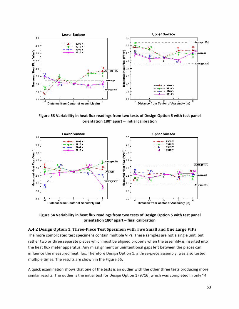
53

Figure 53 Variability in heat flux readings from two tests of Design Option 5 with test panel orientation 180° apart – initial calibration

Figure 54 Variability in heat flux readings from two tests of Design Option 5 with test panel orientation 180° apart – final calibration

A.4.2 Design Option 1, Three-‐Piece Test Specimen with Two Small and One Large VIPs The more complicated test specimens contain multiple VIPs. These samples are not a single unit, but rather two or three separate pieces which must be aligned properly when the assembly is inserted into the heat flux meter apparatus. Any misalignment or unintentional gaps left between the pieces can influence the measured heat flux. Therefore Design Option 1, a three-‐piece assembly, was also tested multiple times. The results are shown in the Figure 55.

A quick examination shows that one of the tests is an outlier with the other three tests producing more similar results. The outlier is the initial test for Design Option 1 (9716) which was completed in only ~4

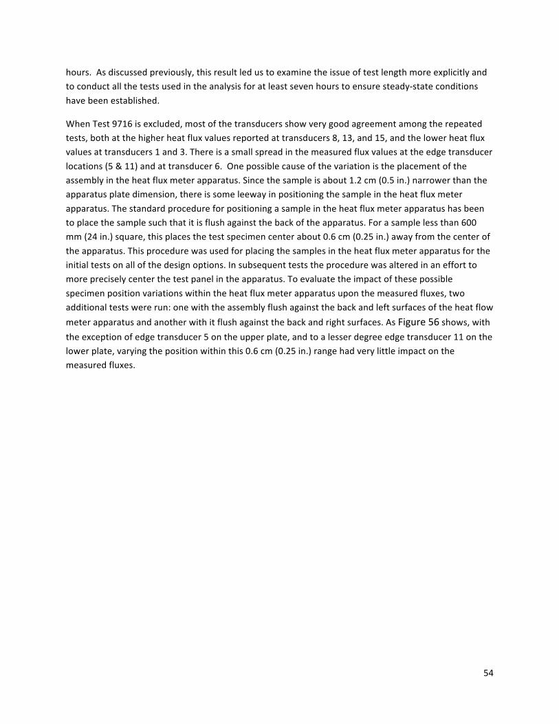
54

hours. As discussed previously, this result led us to examine the issue of test length more explicitly and to conduct all the tests used in the analysis for at least seven hours to ensure steady-‐state conditions have been established.

When Test 9716 is excluded, most of the transducers show very good agreement among the repeated tests, both at the higher heat flux values reported at transducers 8, 13, and 15, and the lower heat flux values at transducers 1 and 3. There is a small spread in the measured flux values at the edge transducer locations (5 & 11) and at transducer 6. One possible cause of the variation is the placement of the assembly in the heat flux meter apparatus. Since the sample is about 1.2 cm (0.5 in.) narrower than the apparatus plate dimension, there is some leeway in positioning the sample in the heat flux meter apparatus. The standard procedure for positioning a sample in the heat flux meter apparatus has been to place the sample such that it is flush against the back of the apparatus. For a sample less than 600 mm (24 in.) square, this places the test specimen center about 0.6 cm (0.25 in.) away from the center of the apparatus. This procedure was used for placing the samples in the heat flux meter apparatus for the initial tests on all of the design options. In subsequent tests the procedure was altered in an effort to more precisely center the test panel in the apparatus. To evaluate the impact of these possible specimen position variations within the heat flux meter apparatus upon the measured fluxes, two additional tests were run: one with the assembly flush against the back and left surfaces of the heat flow meter apparatus and another with it flush against the back and right surfaces. As Figure 56 shows, with the exception of edge transducer 5 on the upper plate, and to a lesser degree edge transducer 11 on the lower plate, varying the position within this 0.6 cm (0.25 in.) range had very little impact on the measured fluxes.

55


56

Figure 56 Impact of test assembly position within the heat flux meter apparatus on measured fluxes for Design Option 1

With centrally located thermal bridges, there is a much greater range of heat flux values in this design option, and the flux distribution is non-‐symmetric, permitting a further comparison of different transducers located over the same position on the test specimen. Additional tests were therefore made with the test specimen rotated 180°. With the exception of the center of the panel (transducer 8), the flux measurements are from different transducers in each orientation as shown in Figure 57. Ideally the measured flux at any location on the panel should be the same for both orientations. Plots of the average fluxes from the multiple runs in each orientation along the midlines of the test specimen are given in. For the original orientation, fluxes from Test 9716 were excluded from the average. HFTs 1 and 15 differ by 5.5% on the lower plate and by 6.6% on the upper plate. Fluxes at all other locations on the assembly are within 5%, and most match much better than 5%.

57

Figure 57 Alternate VIP assembly orientations used in testing

58

Figure 58 Average fluxes along midlines of Design Option 1 from two sets of tests with panel orientations 180° apart

59

Appendix B – List of all Heat Flux Meter Apparatus Tests Test ID Date Design

Option Additional Info Test Time (hours)

9716 11/14/2011 1 Default orientation 4.3† 9932 6/20/2012 1 Rotated 180° 8.6 9936 6/22/2012 1 Default orientation, repeatability check 9.7 9937 6/23/2012 1 Rotated 180°, repeatability check 10.2 9938 6/24/2012 1 Default orientation, repeatability check 9.8 9939 6/25/2012 1 Rotated 180°, repeatability check 8.5 9940 6/25/2012 1 Default orientation, repeatability check 8.1 9941 6/26/2012 1 Rotated 180°, repeatability check 8.4 9942 6/26/2012 1 Default orientation, flush back/left 8.0 9943 6/27/2012 1 Default orientation, flush back/right 9.3 9722 11/15/2011 2 Default orientation 2.8† 9953 7/12/2012 2 Default orientation, repeat 9722 with longer runtime 20.7 9727 11/15/2011 3 Default orientation 2.8† 9954 7/13/2012 3 Default orientation, repeat 9727 with longer runtime 8.6 9763 1/4/2012 4 Default orientation 17.6 9767 1/5/2012 5 Default orientation 24.7 9803 1/19/2012 5 Default orientation, repeatability check 2.9† 9896 5/9/2012 5 Default orientation, heat flow down 24.6 9904 5/14/2012 5 Rotated 90° clockwise 23.3 9907 5/15/2012 5 Default orientation, repeatability check 18.2 9909 5/16/2012 5 Default orientation, repeatability check 15.4 9910 5/17/2012 5 Rotated 180° 8.1 9913 5/17/20212 5 Default orientation, repeatability check 63.3 9776 1/6/2012 6 Default orientation 4.0† 9955 7/13/2012 6 Default orientation, repeat 9776 with longer runtime 8.6 9793 1/13/2012 8 Default orientation 4.8† 9956 7/14/2012 8 Default orientation, repeat 9793 with longer runtime 8.8 9794 1/17/2012 10 Default orientation 4.9† 9963 7/19/2012 10 Default orientation, repeat 9794 with longer runtime 14.6 9800 1/18/2012 11 Default orientation 4.9† 9957 7/15/2012 11 Default orientation, repeat 9800 with longer runtime 8.8 9802 1/18/2012 12 Default orientation 4.8† 9958 7/16/2012 12 Default orientation, repeat 9802 with longer runtime 8.6 9873 4/13/2012 -‐ Small VIP #1 in 305 9875 4/13/2012 -‐ Small VIP #2 in 305 9822 2/10/2012 -‐ Large VIP #1 received 5/11 in 670 9825 2/12/2012 -‐ Large VIP #2 received 5/11 in 670 9785 1/11/2012 -‐ EPS used in panels, 605 9783 1/10/2012 -‐ XPS used in panels, 605 9874 4/13/2012 -‐ Dow EPS from VIP wall tested in RGHB 9898 -‐ Dow VIP assembly from Charleston 9897 -‐ Dow EPS from Charleston

† Insufficient runtime to reliably achieve steady state conditions

60

References

ASTM C1667, Standard Test Method for Using Heat Flow Meter Apparatus to Measure the Center-‐of-‐Panel Thermal Resistivity of Vacuum Panels, ASTM International, 2009.

ASTM C518, Standard Test Method for Steady-‐State Thermal Transmission Properties by Means of the Heat Flow Meter Apparatus, ASTM International, 2010.

ASTM C177, Standard Test Method for Steady-‐State Heat Flux Measurements and Thermal Transmission Properties by Means of the Guarded-‐Hot-‐Plate Apparatus, ASTM International, 2010.

Childs, K.W., 1993, HEATING 7.2 User’s Manual, ORNL/TM-‐12262, Oak Ridge National Laboratory, Oak Ridge, Tennessee

Taylor, B.N., and Kuyatt, C.E., Guidelines for Evaluating and Expressing the Uncertainty of NIST Measurement Results, NIST Technical Note 1297, 1994

Stovall, T. K., Brzezinski, A., “Vacuum Insulation Round-‐Robin to Compare Different Methods of Determining Effective Vacuum Insulation Panel Thermal Resistance,” Insulation Materials: Testing and Applications, Fourth Volume STP 1426, A. Desjarlais, Ed., American Society for Testing and Materials, West Conshohocken, PA 2002.

Taylor, B.N., and C.E. Kuyatt, Guidelines for Evaluating and Expressing the Uncertainty of NIST Measurement Results, NIST Technical Note 1297, National Institute of Standards and Technology, 1994

Wilkes, K. E., et al, “Development of Metal-‐Clad Filled Evacuated Panel Superinsulation,” ORNL/M-‐5871, March 1997.

Wilkes, K. E., et al, “Development of Cladding Materials for Evacuated Panel Superinsulation,” C/ORNL 92-‐0123, November 1999.

exterior insulation systems containing vacuum insulation...

Documents