extracting sub-glottal and supra-glottal features from...

Extracting Sub-glottal and Supra-glottal Features from MFCC usingConvolutional Neural Networks for Speaker Identification in Degraded Audio

Signals

Anurag Chowdhury and Arun RossMichigan State University

[email protected], [email protected]

Abstract

We present a deep learning based algorithm for speakerrecognition from degraded audio signals. We use thecommonly employed Mel-Frequency Cepstral Coefficients(MFCC) for representing the audio signals. A convolutionalneural network (CNN) based on 1D filters, rather than 2Dfilters, is then designed. The filters in the CNN are designedto learn inter-dependency between cepstral coefficients ex-tracted from audio frames of fixed temporal expanse. Ourapproach aims at extracting speaker dependent features,like Sub-glottal and Supra-glottal features, of the humanspeech production apparatus for identifying speakers fromdegraded audio signals. The performance of the proposedmethod is compared against existing baseline schemes onboth synthetically and naturally corrupted speech data. Ex-periments convey the efficacy of the proposed architecturefor speaker recognition.

1. Introduction

Speaker recognition entails determining or verifying theidentity of a speaker from an audio sample [32]. Devel-oping automatic speaker recognition systems that are ro-bust to various types of audio degradations is an open re-search problem. Such systems can benefit a wide varietyof applications ranging from e-commerce and personalizeduser interfaces to surveillance and digital forensics. Popu-lar consumer products such as Alexa [2], Google Home [3],Siri [6], point to the acceptance and demand of speech andspeaker recognition based technologies in the commercialmarket.

In this research, we focus on developing a method fortext-independent speaker identification from degraded au-dio signals.

2. Related WorkSome of the early works [32] in text-independent speaker

identification used Gaussian Mixture Models (GMM) formodeling individual speakers based on the mel-frequencycepstral coefficients (MFCC) of their speech data. Theparameters of the GMM were estimated from the trainingspeech data of each speaker using the Expectation Maxi-mization algorithm.

The GMM based speaker recognition algorithm [32] wasthen extended using adapted Gaussian mixture models [31].The main idea was to train GMM with a large number ofmixtures (256 to 1024), called the Universal BackgroundModel (UBM), to model speaker-independent features. Pa-rameters of the UBM were then adapted using each enrolledspeaker’s training speech data to generate speaker adaptedGMMs.

In order to enable the use of simple metrics suchas cosine similarity for speaker verification, the high-dimensional GMM supervectors were transformed to alower-dimensional space, called the total variability space,using factor analysis [12]. A given speech utterance in thistotal variability space is represented by a low-dimensionalvector called i-vector [13]. The i-vectors are then used forspeaker verification.

Noise in speech signals is a common detrimental factorin the performance of speaker recognition algorithms. Sev-eral spectrum estimation methods [29, 16] and speech en-hancement techniques [27] have been evaluated as front-endprocessing techniques for developing noise robust speakerrecognition methods. Voice activity detection is a techniqueused for detecting parts of the audio with speech activity inthem. Sadjadi et. al. [34] used it is as a front-end process-ing technique for detecting and removing non-speech partsof the audio, which are typically long noisy audio segments.

Over the last decade, speaker recognition in noisy au-dio conditions has become an active area of research inthe speaker recognition community and substantial progresshas been made in the domain.

A. Chowdhury and A. Ross, "Extracting Sub-glottal and Supra-glottal Features from MFCC using Convolutional Neural Networks for Speaker Identification in Degraded Audio Signals,"

Proc. of International Joint Conference on Biometrics (IJCB), (Denver, USA), October 2017.

Additive background noise is the most common type ofnoise encountered in speech signals [28]. Spectral sub-traction is a popular pre-processing technique to removeadditive noise from the speech data. In [38], the authorspropose a robust feature estimation method that can cap-ture source and vocal tract related speech properties fromspectral-substracted noisy speech utterances. Authors usescore level combination of MFCC and Wavelet Octave Co-efficients of Residue (WOCOR) on the pre-processed audiofor performing speaker recognition.

As in the case of speaker recognition from clean speech,MFCC features have been used for describing audio fea-tures of noisy speech signals. Most of the MFCC basedmethods use only the magnitude of the Fourier transformof the speech frames for performing speaker recognition.However, the authors in [37] have shown the benefits of us-ing the phase information along with magnitude to improvethe speaker recognition performance in noisy audio signals.

I-vectors have been extensively used for speaker recogni-tion from noisy audio signals. Authors in [21] improve therobustness of i-vector based speaker verification system byintroducing noisy training data when deriving the i-vectorsand then applying probabilistic linear discriminant analysis(PLDA). In their experiments, the authors confirmed the ef-ficacy of their technique by achieving significant gains inverification accuracy at various signal-to-noise ratio (SNR)levels. Furthermore, the above approach of using i-vectorin conjunction with PLDA was verified to be the best per-forming algorithm even in “ mismatched” noise conditions,where the noise characteristics in the training and testing setwere different [24].

Another work [22], improved upon the effectiveness ofi-vector based speaker recognition methods in the presenceof noisy speech data by using first order Vector Taylor Se-ries (VTS) approximation to extract noise-compensated i-vectors. The approach was inspired by the success of VTSin the field of automatic speech recognition to compensatefor the nonlinear effects of noise in the cepstral domain.

Apart from additive noise, degradation also presents it-self in form of convolutive reverberation in speech audio.The work in [42] addresses this issue in a two staged ap-proach. The authors first use the noisy speech data to traina DNN classifier to produce a binary time-frequency (T-F)mask. The mask is then used to separate out the unreliableT-F units at each audio frame. The masked output audio isthen evaluated using GMM-UBM speaker models, trainedin reverberant environments, to perform speaker recogni-tion.

Another problem associated with speech production innoisy environments is the Lombard effect, where the speak-ers involuntarily tend to increase their vocal effort to makethemselves better audible in noisy environment. This leadsto significant impact on the speaker dependent characteris-

tics of their speech. Authors in [18] have further establishedthe dependence of Lombard speech on noise type and noiselevel using a GMM based Lombard speech type classifier.

In recent years, deep learning techniques have been de-veloped for a large number of classification tasks includingspeaker recognition [25]. Richardson et. al [33] discussedthe training of deep neural networks on frames of spectralaudio features (like MFCC) for performing speaker recog-nition on the input frame. Another approach [33], suggestedusing Deep Neural Networks (DNN) for extracting a featureset from the input audio frames and then using a secondaryneural network classifier for performing speaker recogni-tion using the DNN learnt features. Zhang et. al. [41]trained multi-layer perceptrons and Deep Belief networksfor learning discriminative feature transformations, and de-reverberated features from noisy speech data affected withmicrophone reverberations.

In the following sections, we will discuss the 1-D con-volution filter based convolutional neural network (CNN)we have designed for speaker recognition on considerablydegraded speech data.

3. Rationale behind automatic speaker recog-nition

For performing automatic speaker recognition, it is im-portant to first understand how human speech is generated atthe source. For generating voiced speech sounds, the soundsource is provided by periodic vibration of the vocal foldsby a process known as phonation. For phonation to occur,the ratio of the air pressure below the glottis (sub-glottal)to air pressure above the glottis (supra-glottal) must exceeda certain positive value [1]. The shape and size of the vo-cal tract imparts individuality to a speaker’s voice charac-teristics. MFCC features, as discussed further in the section4.3.1, have been extensively used for capturing acoustic fea-tures of human vocal tract, which we have incorporated inour approach to perform speaker recognition.

Our approach for solving the problem of speakerrecognition uses a Convolutional Neural Network (CNN)uniquely designed to learn the speaker dependent charac-teristics from patches of MFFC audio features. The MFCCfeatures are widely used in the speech and speaker recogni-tion community as they represent the shape of the envelopeof the power spectral density of the speech audio, which inturn is a manifestation of the shape of the human vocal tract.

4. Proposed AlgorithmIn the proposed work, we use 1-D convolutional filters

for learning speaker dependent features from MFCC fea-tures for performing speaker identification in degraded au-dio signals. We model the problem of speaker identificationas an image classification problem and propose a CNN ar-



MFCC Frames

MFC

C F

eatu

res

Figure 1. Visual representation of MFCC feature strip of a cleanaudio clip - TIMIT (first row); corresponding noisy audio clip -Babble (second row); noisy audio clip - F16 (third row); and noisyaudio clip - NTIMIT (fourth row).

chitecture that is uniquely suited for speech data analysisand works particularly well for the task of speaker identifi-cation in degraded audio signals.

4.1. Speech Parametrization

MFCC features are very popular in the speech andspeaker recognition community. A detailed account of theMFCC feature extraction process can be found in [30, 32].We used the VOICEBOX [9] toolbox for extracting MFCCfeature from the audio data. Our 40 dimensional MFCCfeature vector comprises of 20 mel-cepstral coefficients thatincludes the zeroth order coefficient, and 20 first order deltaco-efficients. The hamming window is used in the time do-main and triangular filters are used in the mel-domain.

4.2. Data Organisation

The input audio clip is split into smaller clips, of fixedtemporal expanse, called audio frames. The number ofaudio frames in the input audio clip is determined by thelength of a frame and the frame stride. The length of an au-dio frame, n, is a function of the sampling frequency, fs. Inthe VOICEBOX [9] toolbox, n is expressed as follows:

n = 2blog2(0.03∗fs)c. (1)

The frame stride is chosen to be n/2. We extract 40-dimensional MFCC features per audio frame of an audioclip. Upon extracting the MFCC feature from an audio clip,we obtain a two dimensional feature matrix, which is re-ferred to as MFCC feature strip in this work. Each MFCC

feature strip is of size 40×F , where F is the number of ex-tracted frames. Since the length of the input audio could beof arbitrary length, we extract MFCC feature patches con-taining fixed number of audio frames from the MFCC fea-ture strip of the audio clip. The patches are extracted usinga moving window approach, where the size of the windowis set to 200 frames and the stride value to 100 frames. Avisual representation of the MFCC feature strip of a cleanaudio sample and its corresponding noisy versions can beseen in Figure 1. The MFCC feature patches in the trainingand test sets were modified by subtracting the correspond-ing average image from them, in order to zero-center thedata. The modified MFCC feature patch of size 40 × 200is now used as a two dimensional data input to the CNNnetwork architecture described below.

4.3. 1-D Convolution

A traditional CNN architecture consists of a sequence oflayers. Each layer transforms the input data by applyinglayer specific operations on the input and passing it over tothe next layer. The three most common layer types foundin a CNN architecture are: Convolutional Layer, PoolingLayer and Fully-Connected Layer. The convolutional layerin a CNN is where majority of the learning process takesplace. Design and placement of the filters along the variouslayers of a CNN determine the “concepts” that are learnedat each layer.

Deciding the shape of filters in CNNs is crucial to effec-tively learning the target concept from the input data. Asdiscussed in [23], small square shaped filters are especiallygood for learning local patterns in image data, such as edgesand corners, due to the high correlation between pixels in asmall local neighborhood. However, that is not the case inthe context of MFCC feature strips, as there is no local se-mantic structure (to our knowledge) that can be captured bya 2-D filter. As represented in Figure 1, the pixel valuesalong Y axis corresponding to the MFCC features are on alogarithmic scale, while the pixel values along X axis cor-responding to the time domain are on a linear scale. Hencea 1-D filter is better at learning speaker dependent charac-teristics from the MFCC features placed along the Y axis.

4.3.1 Sub-glottal and Supra-glottal features

In the field of speech recognition, 1-dimensional filtersacross the time variable have shown promising results [40]by effectively learning temporal characteristics in the data.However, in the context of text independent speaker recog-nition, the temporal relevance of speaker dependent char-acteristics across MFCC feature frames is greatly reduced(but not eliminated), as the content of the speech has of-ten no bearing on the identity of the speaker (especially incases where the data is collected in a controlled lab environ-



Figure 2. An illustration of the proposed speaker identification algorithm using 1-D CNN. The input MFCC feature strip is split into MFCCpatches and evaluated on the trained CNN. The classification scores from different patches are fused to arrive at a classification decision.

ment rather than in a natural conversational mode). Hence,learning to extract acoustic speech features that are speakerdependent and text independent, like supra-glottal and sub-glottal resonances [10], are more beneficial for the task ofspeaker identification.

Features of the sub-glottal and supra-glottal vocal tractcapture the acoustics of the trachea-bronchial airways andare known to be noise robust for speaker identification [17].MFCC features, in-turn, are known to capture acousticsof the supra-glottal and sub-glottal vocal tract [7]. Thesefeatures have been reliably estimated from MFCC fea-tures [8], indicating the potential of learning and extractingsuch noise-robust speaker dependent acoustic features fromMFCC feature patches.

The design of our CNN architecture is motivated by theintent to learn and extract such speaker dependent acousticfeatures from MFCC feature patches for speaker identifi-cation. Such acoustic features are usually stable only fora short-period of time, say 20ms, which is effectively cap-tured by the MFCC feature extraction process. Hence, wedesign 1-dimensional convolutional filters of various sizesaligned along the Y axis, as illustrated in Figure 2, in orderto glean the acoustic features resident in mel-cepstral fre-quency coefficients. The final architecture of our CNN ispresented in Figure 3.

4.4. ReLU NonLinearity and Pooling layers

The filter responses from each of the convolutional layersare made to pass through ReLU non-linearity as, unlike sig-moid activation functions, they do not suffer from the prob-lem of vanishing gradients. Further, we used max-poolingto reduce the size of the parameter space to be learnt by the

network.

4.5. Dropout

Dropout layers were added to introduce regularizationin the CNN being trained. It provides the dual benefit ofmaking the CNN robust towards perturbations in the inputdata while also mitigating the problem of over-fitting to thetraining data.

4.6. Score level fusion and Decision

In the testing phase, as illustrated in the Figure 2, theinput MFCC feature strip, X , is split into MFCC patches,xi, iε{1, 2, 3, ..., N}, where, N , is the number of patches.For every input MFCC patch, xi, the CNN gives a set ofclassification scores, {si,j}, jε{1, 2, 3, ..., C}, correspond-ing to the C speakers (e.g., C = 168 in the TIMIT andNTIMIT test datasets). Here, si,j , is the classification scoreassigned to the jth speaker for the ith patch.

Scores from all the patches extracted from the audio clipare then added to give fused classification scores, {Sj}, forthe entire audio clip:

Sj =N∑i=1

si,j ,∀j.

The input audio is then assigned to the speaker j∗ where,

j∗ = argmaxj{Sj}.



Convolutional Layer

Max Pooling Layer

ReLU

Softmax layer

Dropout layer

Fully Connected layerMFCC Feature Patch

40x200x1

9x1

x1@

32

7x1

x32

@6

4

5x1

x64

@1

28

2x1

, Str

ide

2x1

2x1

, Str

ide

2x1

1 X

16

8

1 X

1X

12

8@

16

8

Figure 3. Architecture of the CNN used for Speaker Identification from degraded audio samples. The input is a 40 × 200 × 1 MFCCfeature patch to the CNN. The last layer gives a classification score to each of the 168 speakers in the testing set in the TIMIT and NTIMITdatasets.

Table 1. Identification Results on the SITW, NTIMIT and Noisy variants of TIMIT speech dataset.

Exp. # Training set Testing SetAccuracy (Rank 1 in %) Accuracy (Rank 5 in %)

UBM-GMM

i-vector-PLDA

1-D CNNUBM-GMM

i-vector-PLDA

1-D CNN

1 Babble, F16, R1,V1 Car, Factory, R2, V2 3.86 1.98 32.93 15.57 8.53 65.572 Car, Factory, R2, V2 Babble, F16, R1,V1 9.52 10.61 35.61 21.52 29.26 67.953 Babble, Car, R2, V2 F16, Factory, R1, V1 9.22 14.08 47.61 18.55 31.64 75.094 F16, Factory, R1, V1 Babble, Car, R2, V2 6.84 4.86 38.59 20.13 14.08 66.965 Car, F16, R1, V1 Babble, Factory, R2, V2 6.25 3.27 21.13 15.37 11.01 47.816 Babble, Factory, R2, V2 Car, F16, R1, V1 20.03 10.61 24.60 34.42 31.15 50.997 NTIMIT NTIMIT 52.38 57.14 62.50 81.54 87.5 85.718 SITW SITW 70 49.44 71.11 86.11 73.33 83.33

5. Experiments5.1. Datasets

We used the TIMIT [14] Acoustic-Phonetic ContinuousSpeech Corpus, NTIMIT [20], SITW [26] and Fisher [11]datasets to demonstrate the performance of our algorithmfor text-independent speaker recognition under degradedconditions.

5.1.1 TIMIT Dataset

The TIMIT dataset provides clean speech recordings of 630speakers. There are 462 speakers in the training set and 168speakers in the testing set. The dataset contains of eightmajor dialects of American English. There are ten sessionsof 3 seconds each (so 10 audio samples) per speaker in thedataset. The text spoken by the speakers in the training setand test set are disjoint, making the speaker recognition ex-periments text-independent.

In our experiments, TIMIT dataset was perturbed [5, 19]with synthetic noise of different types (given below) fromthe NOISEX-92 [36] noise dataset. The noisy versions ofthe TIMIT dataset were generated in simulated room envi-ronments with different acoustic properties and reverbera-tion levels, thereby introducing convoluted reverberationsinto the noise profile. The synthetically generated noisydatasets have the following noise characteristics:

1. Noise Type: Following four types of noises were addedto the TIMIT dataset:1.1. F-16: Noise generated by engine of F-16 fighter

aircraft.

1.2. Babble: Noise generated by rapid and continuousbackground human speech.

1.3. Car: Noise generated by engine of a car.1.4. Factory: Noise generated by heavy machinery

operating in a factory environment.2. Signal to Noise Ratio (SNR): The resultant noisy

datasets were each generated at three different SNRlevels, viz., 20 dB, 10dB and 0dB.

3. Room Size: The noisy dataset were generated in a sim-ulated room environment with two different room sizes(4m and 20m, side length of cube), referred to as R1and R2 in the protocol.

4. Reverberation: Two different reverberation coeffi-cients were used to introduce additional noise in thedata, referred to as V1 and V2 in the protocol.

5.1.2 Fisher English Training Speech Part 1 dataset

The Fisher English Training Speech Part 1 Speech datasetcontains conversational speech data collected over tele-phone channels between pairs of speakers. This dataset hasover 12, 000 speakers. Conversations pertaining to a sub-set of 1, 052 speakers from the Fisher dataset were chosenfor the experiments in this work. Audio pertaining to eachspeaker in the conversation is then segmented out and pro-cessed with voice activity detection to remove empty audiosegments from the audio. The audio of each speaker wasthen split into smaller audio snippets of around 3-second du-ration each. We extract 60 audio snippets for each speakerfrom their conversational audio.



Table 2. Identification Results on the Noisy variants of TIMIT speech dataset in presence of the extended gallery-set (1052+168 speakers).The extended gallery consists of audio samples from the Fisher speech dataset also.

Exp. # Training set Testing SetAccuracy (Rank 1 in %) Accuracy (Rank 5 in %)

UBM-GMM

i-vector-PLDA

1-D CNNUBM-GMM

i-vector-PLDA

1-D CNN

1 Babble, F16, R1,V1 Car, Factory, R2, V2 1.58 1.09 13.78 9.92 5.95 35.312 Car, Factory, R2, V2 Babble, F16, R1,V1 1.09 2.87 46.03 2.97 5.75 69.943 Babble, Car, R2, V2 F16, Factory, R1, V1 1.78 5.15 39.68 3.47 13.59 65.574 F16, Factory, R1, V1 Babble, Car, R2, V2 1.88 0.99 37.00 11.30 4.86 57.735 Car, F16, R1, V1 Babble, Factory, R2, V2 0 0.19 24.50 0 0.39 51.196 Babble, Factory, R2, V2 Car, F16, R1, V1 16.56 6.54 51.98 26.19 19.14 72.42

5.1.3 NTIMIT Dataset

NTIMIT [20] dataset consists of speech from the TIMITdataset that was transmitted and re-collected over a tele-phone network. The speech content and speakers in theNTIMIT dataset are identical to that of the TIMIT dataset.But since the NTIMIT is collected over a telephone net-work, it has noise characteristics inherent to the telephonechannel, thereby resulting in a noisy version of the TIMITdataset. Even though the average SNR of NTIMIT dataset ishigher (36dB) than that of the noisy versions of the TIMITdataset that we had created (section 5.1.1), the former pro-vides a much more realistic noise profile.

5.1.4 Speakers in the Wild (SITW) Database

The Speakers in the Wild (SITW) dataset [26] con-tains speech samples collected from open-source mediafor benchmarking and evaluating text-independent speakerrecognition algorithms. Since the SITW data was not col-lected in a controlled setting, it contains real noise, reverber-ation, intra-speaker variability and compression artifacts.There are 299 speakers in the dataset (119 in the trainingset and 180 in the testing set) with variable number of au-dio samples of differing lengths per speaker. Audio of eachspeaker from the dataset is processed with voice activity de-tection to remove any empty audio segments. The audio foreach speaker was then split into smaller audio snippets ofaround 3-second duration each. We extract 10 audio snip-pets for each speaker from their conversational audio.

5.2. Experimental Protocols

In the experiments involving noisy variants of the TIMITdataset, we ensure disjoint noise characteristics in the train-ing and testing sets as shown in Table 1. For example, inexperiment 1, the training set consists of audio samples thatare simulated to be recorded in a room of size R1 and rever-beration coefficient V1, with additive background noise oftype “Babble” and “F16”.

Apart from the six experiments on the noisy TIMITdatasets, we also perform speaker identification experi-ments on the NTIMIT and SITW datasets. The training andthe testing sets in the NTIMIT dataset share the same noise

profile (that of telephone channels), unlike the disjoint noiseprofiles in the noisy versions of TIMIT dataset created byus. The noise content in the SITW datset varies greatly oversamples both within and between different speakers.

Additionally, we also extended the six experiments onthe noisy TIMIT datasets by adopting an extended galleryset comprising of a subset of 1052 speakers from the Fisherdataset alongside the original 168 speakers in the testing setof the TIMIT dataset. The extended gallery set, therefore,has 1220 speakers.

5.2.1 UBM-GMM [31] based Speaker Identification

To obtain baseline performance on the eight experimentslaid out in Table 1, we train a Universal Background Model(UBM) [31] using data from the speakers in the trainingset. The trained UBM is then adapted using data from thespeakers in the test set, to obtained speaker-adapted GMMmodels. For adapting the UBM to individual speakers, nineaudio samples per speaker is used, and the remaining audiosample per speaker is reserved for testing.

5.2.2 i-vector-PLDA [15] based Speaker Identification

To obtain a second baseline performance on the eight ex-periments laid out in Table 1, we train an i-vector-PLDAbased speaker recognition system as implemented in theMSR identity toolkit [35]. Similar to the protocol for theUBM-GMM experiment, we use nine audio samples perspeaker from the testing set for adapting the i-vector mod-els, and the remaining audio sample per speaker is reservedfor evaluation.

5.2.3 1-D CNN based Speaker Identification

The eight experiments, given in Table 1, were then con-ducted using the proposed 1-D CNN based Speaker Iden-tification algorithm. Since the CNN based algorithm doesnot require a background model unlike UBM-GMM [31],we directly train the CNN on the speakers in the test set,with nine audio samples per speaker. The remaining audiosample per speaker is used in the test set.



5.2.4 Extended Gallery Speaker Identification

The six experiments, given in Table 2, are the extendedgallery experiments that were done to test the discriminativepower of the algorithms in presence of an extended galleryset. The speaker recognition models in the six extended-gallery experiments were trained in exactly the same wayas they were done for the first six experiments in Table 1.The gallery set of 168 speakers from the TIMIT dataset areaugmented with a subset of 1052 speakers from the FisherEnglish Training Speech Part 1 Speech dataset. The probedata is sourced from only the 168 speakers in the TIMITdataset. Therefore, for each probe sample, the algorithmsnow have to make a decision from a pool of 1220 speakers,where 168 are from the TIMIT dataset and 1052 are fromthe Fisher dataset.

6. Results and Analysis

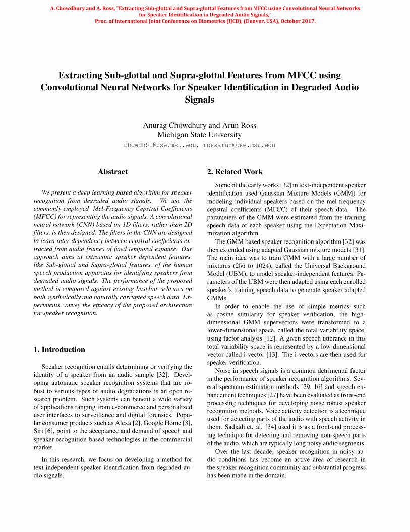
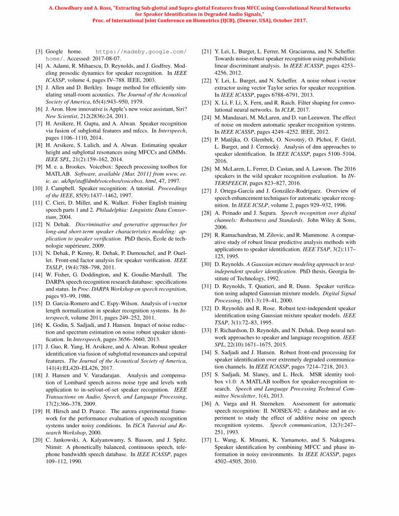
The results of the identification experiments are givenin Tables 1 and 2. Both Rank-1 and Rank-5 identificationaccuracies (in %) are reported for the baseline methods andthe proposed method. The Cumulative Match Characteristic(CMC) curves are given in Figures 4 and 6.• The identification accuracy of the 1-D CNN basedspeaker identification algorithm is vastly superior at Rank1 across all eight experiments in Table 1.• The average identification accuracy across the first sixexperiments on the noisy TIMIT datasets is 33.40% at Rank1 and 62.40% at Rank 5 for 1-D CNN, 9.29% at Rank 1 and20.92% at Rank 5 for UBM-GMM and 7.56% at Rank 1and 20.94% at Rank 5 for i-vector-PLDA.• In the experiments on NTIMIT dataset, it is important tonote that i-vector-PLDA outperforms UBM-GMM at bothRank 1 and Rank 5 indices, and it also outperforms the pro-posed 1-D CNN based algorithm at Rank 5. This could beattributed to the fact that i-vector-PLDA outperforms UBM-GMM in low noise scenarios and, since the NTIMIT datasethas higher average SNR (36dB) compared to that of thenoisy variants of TIMIT dataset (10dB), the i-vector-pldaperforms better on the NTIMIT dataset. Even though thei-vector-PLDA outperforms 1-D CNN at Rank 5, it shouldbe noted that 1-D CNN significantly outperforms i-vector-PLDA at Rank 1.• In the SITW dataset, 1-D CNN based algorithm mod-estly outperforms the baseline algorithms at Rank 1.• In the extended gallery experiments, the accuracy of 1-D CNN based speaker identification algorithm continuesto be superior at both Rank 1 and Rank 5 indices acrossall six experiments. It is noteworthy that in experiment 5,UBM-GMM has a 0% accuracy at both Rank 1 and Rank5, as it completely failed to identify the correct speakers atlower ranks in the extended gallery set. This substantiatesthe challenges of performing speaker identification in large

datasets.• On average, across the first six experiments in Table 1,UBM-GMM, i-vector-PLDA and 1-D CNN correctly iden-tify the same 0.14% of the test samples at Rank 1. 1-D CNNcorrectly identifies an additional 26.60% of the test sam-ples over both the UBM-GMM and i-vector-PLDA basedalgorithms at Rank 1. However, the 1-D CNN based algo-rithm fails to correctly identify 2.64% of the test samplesthat were correctly identified by both the UBM-GMM andi-vector-PLDA based algorithms at Rank 1.• In the seventh experiment in Table 1, on the NTIMITdataset, UBM-GMM, i-vector-PLDA and 1-D CNN basedalgorithms correctly identify the same 41% of the test sam-ples at Rank 1. The 1-D CNN based algorithm correctlyidentifies an additional 10% of the test samples over boththe UBM-GMM and i-vector-PLDA based algorithms atRank 1. However, 1-D CNN based algorithm fails tocorrectly identify 11% of the test samples that were cor-rectly identified by both the UBM-GMM and i-vector-PLDA based algorithms at Rank 1.• In the eigth experiment in Table 1, on the SITW dataset,UBM-GMM, i-vector-PLDA and 1-D CNN based algo-rithms correctly identify the same 41.11% of the test sam-ples at Rank 1. The 1-D CNN based algorithm correctlyidentifies an additional 0.06% of the test samples over boththe UBM-GMM and i-vector-PLDA based algorithms atRank 1. However, the 1-D CNN based algorithm failsto correctly identify 0.02% of the test samples that werecorrectly identified by both the UBM-GMM and i-vector-PLDA based algorithms at Rank 1.• For the experiments with the extended gallery set inTable 2, on average, all three algorithms, UBM-GMM, i-vector-PLDA and 1-D CNN, correctly identified the same0.82% of the test samples at Rank 1. 1-D CNN correctlyidentifies an additional 31.46% of the test samples overboth the UBM-GMM and i-vector-PLDA based algorithmsat Rank 1. However, the 1-D CNN based algorithm failsto correctly identify 0.16% of the test samples that werecorrectly identified by both the UBM-GMM and i-vector-PLDA based algorithms at Rank 1. This establishes thesuperior discriminative power of the 1-D CNN based algo-rithm over both the baseline algorithms.• In both the baseline algorithms and proposed algorithm,the MFCC features are used as input; but the performanceof the 1-D CNN vastly improves over that of the baselines.This suggests that the 1-D CNN is better at extracting im-portant speaker dependent characteristics, like sub-glottaland supra-glottal features, in presence of audio degrada-tions.

7. Conclusion and Future GoalsDegradations in speech audio can distort and mask the

speaker dependent characteristics in the audio signal. Tra-



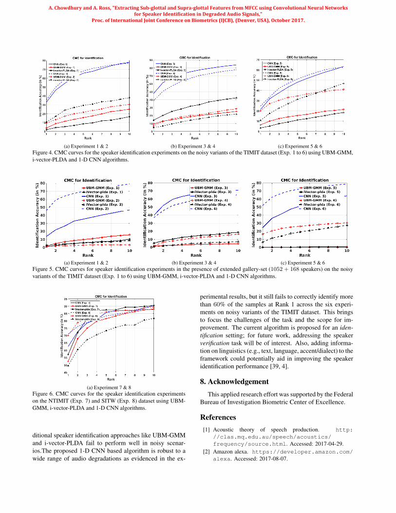
(a) Experiment 1 & 2 (b) Experiment 3 & 4 (c) Experiment 5 & 6Figure 4. CMC curves for the speaker identification experiments on the noisy variants of the TIMIT dataset (Exp. 1 to 6) using UBM-GMM,i-vector-PLDA and 1-D CNN algorithms.

(a) Experiment 1 & 2 (b) Experiment 3 & 4 (c) Experiment 5 & 6Figure 5. CMC curves for speaker identification experiments in the presence of extended gallery-set (1052 + 168 speakers) on the noisyvariants of the TIMIT dataset (Exp. 1 to 6) using UBM-GMM, i-vector-PLDA and 1-D CNN algorithms.

(a) Experiment 7 & 8Figure 6. CMC curves for the speaker identification experimentson the NTIMIT (Exp. 7) and SITW (Exp. 8) dataset using UBM-GMM, i-vector-PLDA and 1-D CNN algorithms.

ditional speaker identification approaches like UBM-GMMand i-vector-PLDA fail to perform well in noisy scenar-ios.The proposed 1-D CNN based algorithm is robust to awide range of audio degradations as evidenced in the ex-

perimental results, but it still fails to correctly identify morethan 60% of the samples at Rank 1 across the six experi-ments on noisy variants of the TIMIT dataset. This bringsto focus the challenges of the task and the scope for im-provement. The current algorithm is proposed for an iden-tification setting; for future work, addressing the speakerverification task will be of interest. Also, adding informa-tion on linguistics (e.g., text, language, accent/dialect) to theframework could potentially aid in improving the speakeridentification performance [39, 4].

8. AcknowledgementThis applied research effort was supported by the Federal

Bureau of Investigation Biometric Center of Excellence.

References[1] Acoustic theory of speech production. http:

//clas.mq.edu.au/speech/acoustics/frequency/source.html. Accessed: 2017-04-29.

[2] Amazon alexa. https://developer.amazon.com/alexa. Accessed: 2017-08-07.



[3] Google home. https://madeby.google.com/home/. Accessed: 2017-08-07.

[4] A. Adami, R. Mihaescu, D. Reynolds, and J. Godfrey. Mod-eling prosodic dynamics for speaker recognition. In IEEEICASSP, volume 4, pages IV–788. IEEE, 2003.

[5] J. Allen and D. Berkley. Image method for efficiently sim-ulating small-room acoustics. The Journal of the AcousticalSociety of America, 65(4):943–950, 1979.

[6] J. Aron. How innovative is Apple’s new voice assistant, Siri?New Scientist, 212(2836):24, 2011.

[7] H. Arsikere, H. Gupta, and A. Alwan. Speaker recognitionvia fusion of subglottal features and mfccs. In Interspeech,pages 1106–1110, 2014.

[8] H. Arsikere, S. Lulich, and A. Alwan. Estimating speakerheight and subglottal resonances using MFCCs and GMMs.IEEE SPL, 21(2):159–162, 2014.

[9] M. e. a. Brookes. Voicebox: Speech processing toolbox forMATLAB. Software, available [Mar. 2011] from www. ee.ic. ac. uk/hp/staff/dmb/voicebox/voicebox. html, 47, 1997.

[10] J. Campbell. Speaker recognition: A tutorial. Proceedingsof the IEEE, 85(9):1437–1462, 1997.

[11] C. Cieri, D. Miller, and K. Walker. Fisher English trainingspeech parts 1 and 2. Philadelphia: Linguistic Data Consor-tium, 2004.

[12] N. Dehak. Discriminative and generative approaches forlong-and short-term speaker characteristics modeling: ap-plication to speaker verification. PhD thesis, Ecole de tech-nologie superieure, 2009.

[13] N. Dehak, P. Kenny, R. Dehak, P. Dumouchel, and P. Ouel-let. Front-end factor analysis for speaker verification. IEEETASLP, 19(4):788–798, 2011.

[14] W. Fisher, G. Doddington, and K. Goudie-Marshall. TheDARPA speech recognition research database: specificationsand status. In Proc. DARPA Workshop on speech recognition,pages 93–99, 1986.

[15] D. Garcia-Romero and C. Espy-Wilson. Analysis of i-vectorlength normalization in speaker recognition systems. In In-terspeech, volume 2011, pages 249–252, 2011.

[16] K. Godin, S. Sadjadi, and J. Hansen. Impact of noise reduc-tion and spectrum estimation on noise robust speaker identi-fication. In Interspeech, pages 3656–3660, 2013.

[17] J. Guo, R. Yang, H. Arsikere, and A. Alwan. Robust speakeridentification via fusion of subglottal resonances and cepstralfeatures. The Journal of the Acoustical Society of America,141(4):EL420–EL426, 2017.

[18] J. Hansen and V. Varadarajan. Analysis and compensa-tion of Lombard speech across noise type and levels withapplication to in-set/out-of-set speaker recognition. IEEETransactions on Audio, Speech, and Language Processing,17(2):366–378, 2009.

[19] H. Hirsch and D. Pearce. The aurora experimental frame-work for the performance evaluation of speech recognitionsystems under noisy conditions. In ISCA Tutorial and Re-search Workshop, 2000.

[20] C. Jankowski, A. Kalyanswamy, S. Basson, and J. Spitz.Ntimit: A phonetically balanced, continuous speech, tele-phone bandwidth speech database. In IEEE ICASSP, pages109–112, 1990.

[21] Y. Lei, L. Burget, L. Ferrer, M. Graciarena, and N. Scheffer.Towards noise-robust speaker recognition using probabilisticlinear discriminant analysis. In IEEE ICASSP, pages 4253–4256, 2012.

[22] Y. Lei, L. Burget, and N. Scheffer. A noise robust i-vectorextractor using vector Taylor series for speaker recognition.In IEEE ICASSP, pages 6788–6791, 2013.

[23] X. Li, F. Li, X. Fern, and R. Raich. Filter shaping for convo-lutional neural networks. In ICLR, 2017.

[24] M. Mandasari, M. McLaren, and D. van Leeuwen. The effectof noise on modern automatic speaker recognition systems.In IEEE ICASSP, pages 4249–4252. IEEE, 2012.

[25] P. Matejka, O. Glembek, O. Novotny, O. Plchot, F. Grezl,L. Burget, and J. Cernocky. Analysis of dnn approaches tospeaker identification. In IEEE ICASSP, pages 5100–5104,2016.

[26] M. McLaren, L. Ferrer, D. Castan, and A. Lawson. The 2016speakers in the wild speaker recognition evaluation. In IN-TERSPEECH, pages 823–827, 2016.

[27] J. Ortega-Garcıa and J. Gonzalez-Rodrıguez. Overview ofspeech enhancement techniques for automatic speaker recog-nition. In IEEE ICSLP, volume 2, pages 929–932, 1996.

[28] A. Peinado and J. Segura. Speech recognition over digitalchannels: Robustness and Standards. John Wiley & Sons,2006.

[29] R. Ramachandran, M. Zilovic, and R. Mammone. A compar-ative study of robust linear predictive analysis methods withapplications to speaker identification. IEEE TSAP, 3(2):117–125, 1995.

[30] D. Reynolds. A Gaussian mixture modeling approach to text-independent speaker identification. PhD thesis, Georgia In-stitute of Technology, 1992.

[31] D. Reynolds, T. Quatieri, and R. Dunn. Speaker verifica-tion using adapted Gaussian mixture models. Digital SignalProcessing, 10(1-3):19–41, 2000.

[32] D. Reynolds and R. Rose. Robust text-independent speakeridentification using Gaussian mixture speaker models. IEEETSAP, 3(1):72–83, 1995.

[33] F. Richardson, D. Reynolds, and N. Dehak. Deep neural net-work approaches to speaker and language recognition. IEEESPL, 22(10):1671–1675, 2015.

[34] S. Sadjadi and J. Hansen. Robust front-end processing forspeaker identification over extremely degraded communica-tion channels. In IEEE ICASSP, pages 7214–7218, 2013.

[35] S. Sadjadi, M. Slaney, and L. Heck. MSR identity tool-box v1.0: A MATLAB toolbox for speaker-recognition re-search. Speech and Language Processing Technical Com-mittee Newsletter, 1(4), 2013.

[36] A. Varga and H. Steeneken. Assessment for automaticspeech recognition: II. NOISEX-92: a database and an ex-periment to study the effect of additive noise on speechrecognition systems. Speech communication, 12(3):247–251, 1993.

[37] L. Wang, K. Minami, K. Yamamoto, and S. Nakagawa.Speaker identification by combining MFCC and phase in-formation in noisy environments. In IEEE ICASSP, pages4502–4505, 2010.



[38] N. Wang, P. Ching, N. Zheng, and T. Lee. Robust speakerrecognition using both vocal source and vocal tract featuresestimated from noisy input utterances. In IEEE InternationalSymposium on Signal Processing and Information Technol-ogy, pages 772–777, 2007.

[39] J. Wolf. Efficient acoustic parameters for speaker recog-nition. The Journal of the Acoustical Society of America,51(6B):2044–2056, 1972.

[40] X. Zhang and Y. LeCun. Text understanding from scratch.CoRR, abs/1502.01710, 2015.

[41] Z. Zhang, L. Wang, A. Kai, T. Yamada, W. Li, and M. Iwa-hashi. Deep neural network-based bottleneck feature anddenoising autoencoder-based dereverberation for distant-talking speaker identification. EURASIP Journal on Audio,Speech, and Music Processing, 2015(1):12, 2015.

[42] X. Zhao, Y. Wang, and D. Wang. Robust speaker iden-tification in noisy and reverberant conditions. IEEE/ACMTransactions on Audio, Speech and Language Processing,22(4):836–845, 2014.



extracting sub-glottal and supra-glottal features from...

Documents