Extracting the relevant trends for applied portfolio

management

Theo Berger∗

January 13, 2017

Abstract

As financial return series comprise relevant information about risk and depen-

dence, historical return series describe the underlying information for applied

portfolio management. Although market quotes are measured periodically,

the data contains information on short-run as well as long-run trends of the

underlying return series. A simulation study and an analysis of daily mar-

ket prices reveal the relevance of short-run information for applied portfolio

management.

JEL-Classification: C10, C32, G11, G15

Keywords: Wavelet decomposition, short-run trends, portfolio

management

∗University of Bremen, Department of Business and Administration, Chair of Applied Statisticsand Empirical Economics, D-28359 Bremen, email: thberger@uni-bremen.de, phone: (0049)-421-218-66903, fax:(0049)-421-218-66902.

1 Introduction

Historical market prices describe the underlying information of financial risk man-

agement. Although, financial data is tracked periodically, i.e. daily, weekly or

monthly, historical market prices comprise information on both short- and long-run

seasonalities of the underlying return series. This paper decomposes financial re-

turn series into different seasonalities and provides an assessment of the relevance

of particular seasonalities for daily portfolio management.

In order to decompose financial return series into its underlying trends, Percival

and Walden (2000) and Gencay et al. (2001) introduced wavelet decomposition to

financial return series and triggered a growing field of literature which deals with

decomposition of financial return series into short-run and long-run seasonalities.

In this context, Gencay et al. (2003) and Gencay et al. (2005) apply the Capital

Asset Pricing Model (CAPM) to decomposed return series of international stock in-

dices and illustrate that systematic risk increases for long-run seasonalities. Rua and

Nunes (2012) confirm this finding for emerging markets, whereas Gallegati (2012)

decomposes return series of stock market indices of the G7 countries, Brazil and

Hong Kong to assess changing correlation regimes between decomposed return se-

ries. As a result, dependence schemes between decomposed return series are de-

scribed by different patterns, especially dependence between long-run seasonalities

appears to be stronger than suggested by the original data. Reboredo and Rivera-

Castro (2014) assess dependence between decomposed European and US stock and

oil prices and find evidence of increased dependence between long-run seasonalities

after 2008. Dewandaru et al. (2015) analyze dependence between Asian stocks;

Andries et al. (2014) between interest rates, stock prices and exchange rates; Berger

and Salah Uddin (2016) dependence between commodities; and Tan et al. (2014)

analyze dependence between US and Asian equity markets.

As dependence between assets presents crucial information in the context of

periodical portfolio allocations, financial portfolios are impacted by misspecified

2

dependence parameters (see Fantazzini 2009). Moreover, according to Ane and

Kharoubi (2003), misspecified dependence structure accounts for (up to) 20% of the

overall portfolio risk.

In this vein, the wavelet decomposition of financial return series implies a de-

composition of variance and covariance of the underlying return series, namely the

relevant information for applied portfolio management. Consequently, the decom-

position of return series leads to a decomposition of both the risk of an asset (con-

ditional variance) and diversification effects between assets (covariance), whereas

information on different seasonalities (i.e. short run, middle run and long run in-

formation) directly impacts portfolio allocations. Furthermore, wavelet analysis not

only allows for a decomposition but also for a reconstruction of a decomposed finan-

cial return series and as presented by Berger and Gencay (2016), return series can

be reconstructed by excluding particular seasonalities.

Triggered by the ongoing discussion on dependence structure between decom-

posed return series, we introduce decomposed information on long-run and short-run

seasonalities to periodical portfolio management and evaluate the relevance of dif-

ferent seasonalities within an out-of-sample analysis. Doing so allows us to evaluate

the relevance of changing dependence schemes between decomposed financial time

series for applied portfolio management.

In doing so, we draw on Berger and Genccay (2016) and apply wavelet filter to

decompose return series into different components and reconstruct the return series,

which enables us to exclusively take particular trends into account. That is, we

reconstruct filtered return series by taking either short-run, middle-run or long-run

seasonalities into account. Furthermore, we apply the reconstructed versions of the

original return series to build portfolio allocations and assess their out-of-sample

performance. The assessment will be twofold:

First, we set up a simulation analysis, and simulate return series which are

described by different patterns of long-memory effects to assess the relevance of

3

short- and long-memory of a return series on portfolio allocations. By investigating

reconstructed return series which take either short-run or long-run memory into

account, we shed light on the relevant information for applied portfolio management

in the absence of incomplete information on the underlying market conditions.

Second, we assess the out-of-sample performance of global mean variance efficient

portfolios which are based on reconstructed return series and compare the perfor-

mance with the mean-variance efficient portfolio allocations based on un-decomposed

daily data. To take account of different market sizes and regimes, we assess stocks

that are listed at leading indices of both developed and emerging stock markets. The

results indicate that middle-run and long-run information can be excluded from the

original time series without impacting the out-of-sample performance of daily port-

folio management.

The following is structured as follows. Section 2 describes the relevant method-

ology and the simulation study is presented in Section 3. Results regarding the

empirical portfolio analysis are given in section 4 and section 5 concludes.

4

2 Methodology

In this section, we present methodological approach of wavelet filtering that enables

us to decompose and reconstruct the underlying return series. In addition, we intro-

duce the portfolio allocation algorithm which will be applied to the reconstructed

return series and relevant quality criteria of our analysis.

2.1 Maximal overlap discrete wavelet transform

In this section, we introduce the maximal overlap discrete wavelet transform (MODWT)

as described by Gencay et al. (2001) and Percival and Walden (2000)1. MODWT

approach describes an expansion of the classical approach of discrete wavelet trans-

formation (DWT) (see Zhu et al. 2014). As the number of observations remains

constant at each level of decomposition2 and is characterized by shift invariance, the

MODWT approach is predestined for a rolling window out-of-sample analysis.

As presented by Gencay et al. (2001), the choice of wavelet filter is directly

linked to a scaling filter and describes the core of wavelet decomposition.

Let hj,l be the DWT wavelet filter with l = 1, ..., L describing the length of the

filter and j = 1, ..., J the level of decomposition, then the corresponding scaling filter

is determined by gj,l .3

Further, as the MODWT filter describes an expansion of the DWT concept, the

MODWT wavelet and scaling filter are directly obtained from DWT filters by:

hj,l = hj,l/2j/2, (1)

and

gj,l = gj,l/2j/2. (2)

1In contradiction to Fourier Analysis, the decomposition of a return series via wavelet approachevents can still be localized throughout the decompositions.

2Due to boundary conditions, only the observations at the beginning of each series are reduced.3The respective scaling (low pass) filter gj,l, depends on hj,l by quadratic mirror filtering and

is given by gl = −1lhl.

5

In this vein, as the underlying data of this study is described by daily return

series, r = rt, t = 0, 1, 2, ..., N − 1, to decompose the series into J frequencies,

wavelet coefficients of level j are achieved by the convolution of r and the MODWT

filters (see Percival and Walden 2000) :

Wj,t =Lj−1∑l=0

hj,lrt−l mod N , (3)

and

Vj,t =Lj−1∑l=0

gj,lrt−l mod N . (4)

with Lj = (2j − 1)(L − 1) + 1. According to the presented MODWT, wavelet

coefficients at all scales are characterized by the same number of observations as the

original return series r and can be expressed in matrix notation :

Wj = ωjr (5)

and

Vj = vjr. (6)

As we aim to utilize MODWT for an out-of-sample portfolio application, we are

interested in the maximum number of boundary-free coefficients. Therefore, we

use the Haar filter which has the smallest number of coefficients leading to h1,0 =12 , h1,1 = −1

2 and g1,0 = 12 , g1,1 = 1

2 for j = 1.

Due to the fact that our study aims at the exclusion of particular seasonalities

from the original return series, we make use of the properties of wavelet analysis

that allow for a reconstruction of the decomposed series. Thus, based on the DWT

specific concept of multi-resolution analysis (MRA), the underlying original return

series can be reconstructed by simply summing up all coefficients and the smoothed

6

version of decomposition step J :

r =J∑j=1

ωTj Wj + vTJ VJ =J∑j=1

Dj + SJ . (7)

In this setup Dj = ωTj Wj describes the detail coefficients and SJ = vTj VJ the corre-

sponding smoothed version of the return series. Further, Dj functions as the local

details of the trend at level j and captures the short term dynamics (low levels)

of the original return series whereas long-term fluctuations are described by high

levels. Consequently, SJ is defined as the smoothed version of the time series.

Based on the introduced setup, which allows for a decomposition and recon-

struction of the underlying return series, we follow Berger and Gencay (2016) and

reconstruct decomposed return series by excluding particular levels of decomposi-

tion.

Hence, after a return series is decomposed into J scales, we reconstruct the

series by excluding the highest scales that comprise the long-run information of the

underlying return series. More concretely, in our analysis, we decompose every series

eight times and discuss three different reconstructed versions of the original return

series4:

rSR =3∑j=1

Dj, (8)

rMR =5∑j=4

Dj, (9)

rLR =8∑j=6

Dj. (10)

Consequently, based on eight decomposition levels of the original return series, we

achieve the reconstructed return series that exclusively comprises short-run infor-

mation (rSR) by summing up the relevant detail coefficients D1, D2, D3. rMR the

middle-run trend and rLR the long-run trend are constructed in the same way. For

a thorough introduction to MODWT in the context of financial data we refer to4We refer to Table ?? for an economic discussion of the applied setup.

7

Gencay et al. (2001) and for an intuitive economic introduction to wavelet analysis

we refer to Crowley (2007).

2.2 Portfolio allocation

Based on historical financial return series, including its filtered versions (see equa-

tions (8)-(9)), we introduce the competing versions of the original return series

(comprising short run, middle run and long run respectively), to applied portfolio

management.

Due to the focus on the return series, we apply the covariance matrices of the

reconstructed return series to the widely accepted Markowitz portfolio optimiza-

tion setup (see Markowitz 1952) and assess the global minimum-variance allocation,

whereby we restrict our analysis to the absence of short sellings:

minwt

wTt Htwt s.t. 1TNwt = 1. (11)

In this setup, only the estimate of the covariance matrix (Ht) of the underlying

series (either original or reconstructed) impacts portfolio allocations. As this strat-

egy ignores expected returns, differences between portfolio allocations are directly

linked to differences in the underlying covariance matrices5.

In order to discuss the relevance of the underlying covariance matrices which con-

tain information on different memories, we assess the out-of-sample performance of

the global mean variance efficient portfolio allocation by several backtesting criteria.

Analogous to the study of De Miguel et al. (2009), we also evaluate the out-of-

sample returns by different performance metrics.

In order to compare portfolio allocations which aim at minimizing particular

trends, we define allocations based on un-decomposed data as the benchmark and

assess the information ratio of strategy k against a benchmark b strategy. As pre-

5Berger (2016) initiated the application of decomposed return series to applied portfolio man-agement.

8

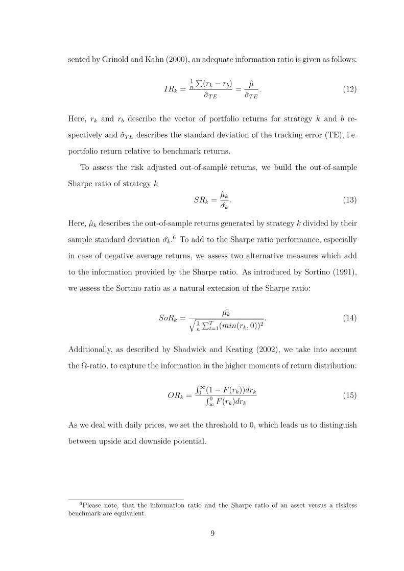
sented by Grinold and Kahn (2000), an adequate information ratio is given as follows:

IRk =1n

∑(rk − rb)σTE

= µ

σTE. (12)

Here, rk and rb describe the vector of portfolio returns for strategy k and b re-

spectively and σTE describes the standard deviation of the tracking error (TE), i.e.

portfolio return relative to benchmark returns.

To assess the risk adjusted out-of-sample returns, we build the out-of-sample

Sharpe ratio of strategy k

SRk = µkσk. (13)

Here, µk describes the out-of-sample returns generated by strategy k divided by their

sample standard deviation σk.6 To add to the Sharpe ratio performance, especially

in case of negative average returns, we assess two alternative measures which add

to the information provided by the Sharpe ratio. As introduced by Sortino (1991),

we assess the Sortino ratio as a natural extension of the Sharpe ratio:

SoRk = µk√1n

∑Tt=1(min(rk, 0))2

. (14)

Additionally, as described by Shadwick and Keating (2002), we take into account

the Ω-ratio, to capture the information in the higher moments of return distribution:

ORk =∫∞

0 (1− F (rk))drk∫ 0∞ F (rk)drk

(15)

As we deal with daily prices, we set the threshold to 0, which leads us to distinguish

between upside and downside potential.

6Please note, that the information ratio and the Sharpe ratio of an asset versus a risklessbenchmark are equivalent.

9

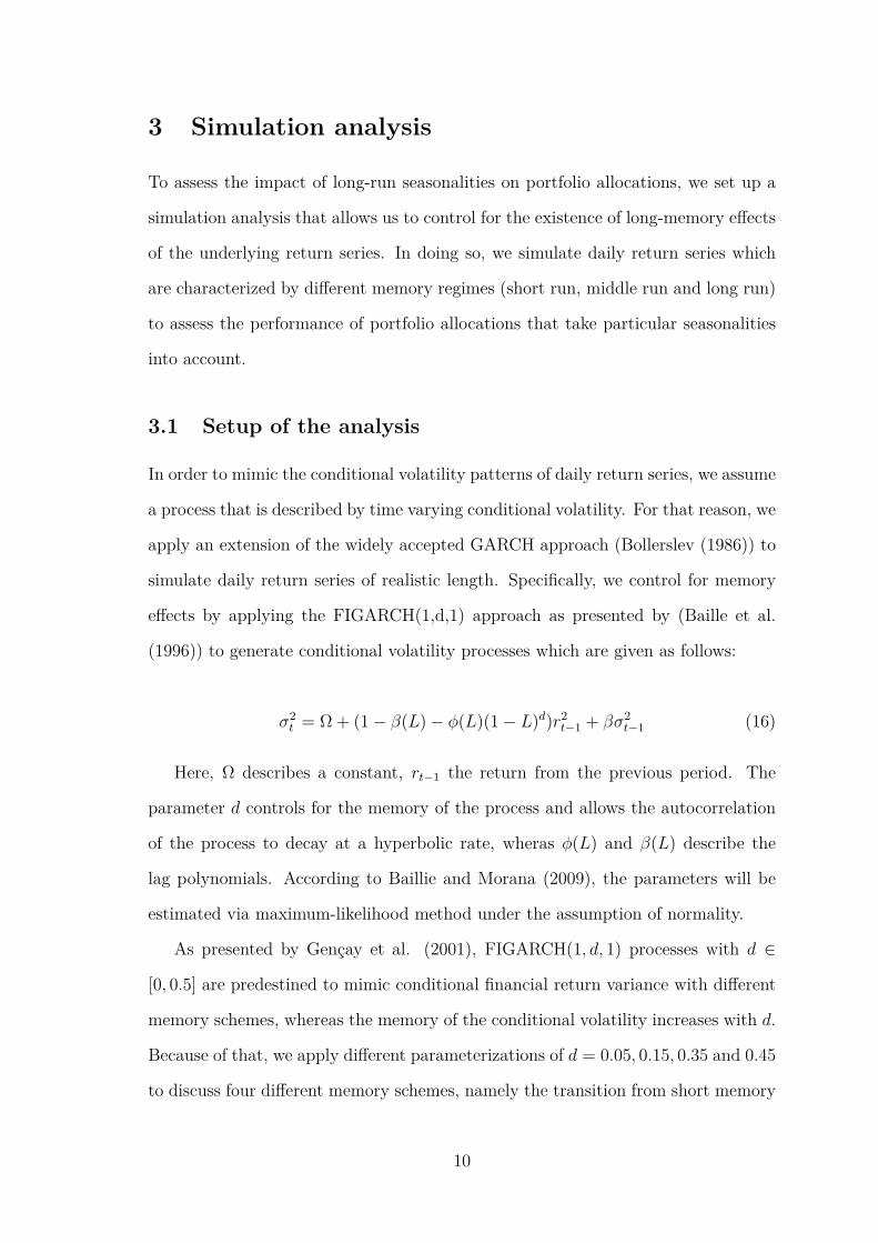
3 Simulation analysis

To assess the impact of long-run seasonalities on portfolio allocations, we set up a

simulation analysis that allows us to control for the existence of long-memory effects

of the underlying return series. In doing so, we simulate daily return series which

are characterized by different memory regimes (short run, middle run and long run)

to assess the performance of portfolio allocations that take particular seasonalities

into account.

3.1 Setup of the analysis

In order to mimic the conditional volatility patterns of daily return series, we assume

a process that is described by time varying conditional volatility. For that reason, we

apply an extension of the widely accepted GARCH approach (Bollerslev (1986)) to

simulate daily return series of realistic length. Specifically, we control for memory

effects by applying the FIGARCH(1,d,1) approach as presented by (Baille et al.

(1996)) to generate conditional volatility processes which are given as follows:

σ2t = Ω + (1− β(L)− φ(L)(1− L)d)r2

t−1 + βσ2t−1 (16)

Here, Ω describes a constant, rt−1 the return from the previous period. The

parameter d controls for the memory of the process and allows the autocorrelation

of the process to decay at a hyperbolic rate, wheras φ(L) and β(L) describe the

lag polynomials. According to Baillie and Morana (2009), the parameters will be

estimated via maximum-likelihood method under the assumption of normality.

As presented by Gencay et al. (2001), FIGARCH(1, d, 1) processes with d ∈

[0, 0.5] are predestined to mimic conditional financial return variance with different

memory schemes, whereas the memory of the conditional volatility increases with d.

Because of that, we apply different parameterizations of d = 0.05, 0.15, 0.35 and 0.45

to discuss four different memory schemes, namely the transition from short memory

10

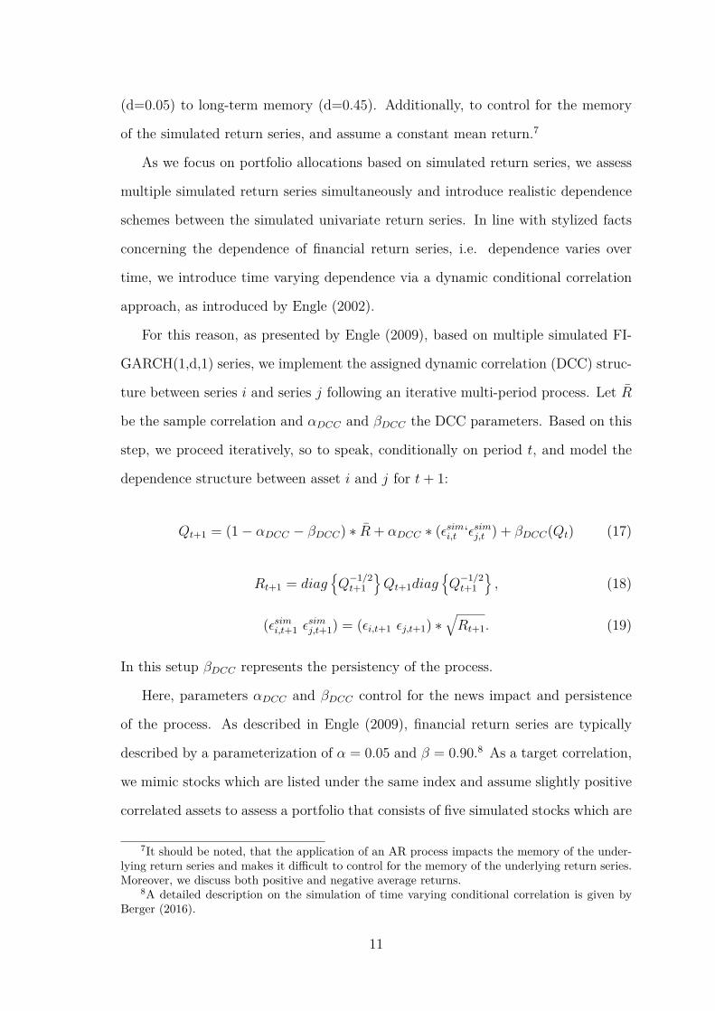
(d=0.05) to long-term memory (d=0.45). Additionally, to control for the memory

of the simulated return series, and assume a constant mean return.7

As we focus on portfolio allocations based on simulated return series, we assess

multiple simulated return series simultaneously and introduce realistic dependence

schemes between the simulated univariate return series. In line with stylized facts

concerning the dependence of financial return series, i.e. dependence varies over

time, we introduce time varying dependence via a dynamic conditional correlation

approach, as introduced by Engle (2002).

For this reason, as presented by Engle (2009), based on multiple simulated FI-

GARCH(1,d,1) series, we implement the assigned dynamic correlation (DCC) struc-

ture between series i and series j following an iterative multi-period process. Let R

be the sample correlation and αDCC and βDCC the DCC parameters. Based on this

step, we proceed iteratively, so to speak, conditionally on period t, and model the

dependence structure between asset i and j for t+ 1:

Qt+1 = (1− αDCC − βDCC) ∗ R + αDCC ∗ (εsimi,t ‘εsimj,t ) + βDCC(Qt) (17)

Rt+1 = diagQ−1/2t+1

Qt+1diag

Q−1/2t+1

, (18)

(εsimi,t+1 εsimj,t+1) = (εi,t+1 εj,t+1) ∗

√Rt+1. (19)

In this setup βDCC represents the persistency of the process.

Here, parameters αDCC and βDCC control for the news impact and persistence

of the process. As described in Engle (2009), financial return series are typically

described by a parameterization of α = 0.05 and β = 0.90.8 As a target correlation,

we mimic stocks which are listed under the same index and assume slightly positive

correlated assets to assess a portfolio that consists of five simulated stocks which are

7It should be noted, that the application of an AR process impacts the memory of the under-lying return series and makes it difficult to control for the memory of the underlying return series.Moreover, we discuss both positive and negative average returns.

8A detailed description on the simulation of time varying conditional correlation is given byBerger (2016).

11

characterized by a correlation matrix as follows:

R =

1 0.8 0.4 0.3 0.5

1 0.2 0.1 0.3

1 0.4 0.1

1 0.7

1

(20)

Based on the simulated return series, we decompose each series into three differ-

ent trends, as described by equations (7) - (10) in section 2.1 . Then, we estimate

the mean-var efficient portfolio allocations (equation (11)) based on the decomposed

and the original return series and analyze the out-of-sample performance of each al-

location strategy via rolling window analysis.

The setup of the simulation study can be summarized as follows:

1) We generate five return series comprising 1,500 observations via FIGARCH(1,d,1)

approach.

2) We introduce time varying conditional correlation via DCC approach.

3) We decompose each return series via MODWT approach.

4) We reconstruct the decomposed return series and achieve rsimSR , rsimMR and rsimLR

and the simulated return series rsim and assess 500 -1,500.

5) We apply rolling window approach: 1+t:500+t.

6) We apply Markowitz approach.

7) We assess the out-of-sample performance.

For each parameterization of d we repeat the simulation 1,000 times to assess the

robustness of the results.

12

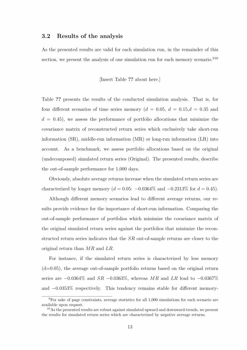
3.2 Results of the analysis

As the presented results are valid for each simulation run, in the remainder of this

section, we present the analysis of one simulation run for each memory scenario.910

[Insert Table ?? about here.]

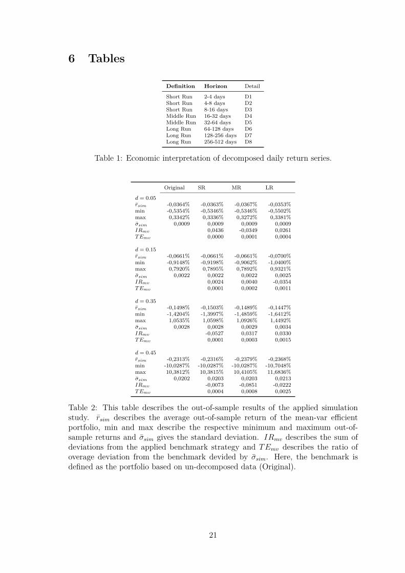
Table ?? presents the results of the conducted simulation analysis. That is, for

four different scenarios of time series memory (d = 0.05, d = 0.15,d = 0.35 and

d = 0.45), we assess the performance of portfolio allocations that minimize the

covariance matrix of reconstructed return series which exclusively take short-run

information (SR), middle-run information (MR) or long-run information (LR) into

account. As a benchmark, we assess portfolio allocations based on the original

(undecomposed) simulated return series (Original). The presented results, describe

the out-of-sample performance for 1,000 days.

Obviously, absolute average returns increase when the simulated return series are

characterized by longer memory (d = 0.05: −0.0364% and −0.2313% for d = 0.45).

Although different memory scenarios lead to different average returns, our re-

sults provide evidence for the importance of short-run information. Comparing the

out-of-sample performance of portfolios which minimize the covariance matrix of

the original simulated return series against the portfolios that minimize the recon-

structed return series indicates that the SR out-of-sample returns are closer to the

original return than MR and LR.

For instance, if the simulated return series is characterized by less memory

(d=0.05), the average out-of-sample portfolio returns based on the original return

series are −0.0364% and SR −0.0363%, whereas MR and LR lead to −0.0367%

and −0.0353% respectively. This tendency remains stable for different memory-

9For sake of page constraints, average statistics for all 1,000 simulations for each scenario areavailable upon request.

10As the presented results are robust against simulated upward and downward-trends, we presentthe results for simulated return series which are characterized by negative average returns.

13

scenarios, indicating that information on the short-run memory of a return series

provides the relevant information for portfolio allocations.

The applied information ratio (IRmv) allows for a comparison of the portfolio

strategies vis-a-vis the applied benchmark (Original). In this particular simula-

tion setup, lower info ratios are preferred vis-a-vis higher values, indicating that

the assessed strategy does not deviate from the out-of-sample returns based on

un-decomposed return series. The results suggest, that SR leads to out-of-sample

returns which are closest to the benchmark, whereas MR and LR result in larger

deviations from the benchmark and to more volatile out-of-sample returns. This

finding indicates that the relevant information for daily portfolio management can

be described by decomposed short-run trends. Moreover, the results of the presented

simulation study demonstrate that the long-run information can be excluded from

the underlying return series without impacting portfolio allocations.

Although simulated return series are characterized by long-memory schemes (d =

0.45), minimizing the covariance matrix of the reconstructed return series which

exclusively comprises information on the short-run trends of the original series leads

to a similar out-of-sample performance, according to its benchmark.

14

4 Empirical Study

4.1 Data

The data set of the empirical study comprises different stocks which are listed under

leading indices of nine different countries. In order to indicate robustness of the

empirical results, we analyze different currency denominations and focus on both

developed and emerging markets. We discuss assets which are listed on the leading

North American, German and British stock markets as representatives of developed

markets. Additionally, we assess Canadian and Australian stocks as representatives

for smaller indexes. To analyze emerging markets, we stick to the definition of

O’Neil (2001) and assess stocks which are listed under the leading indices of the so

called BRIC states. That is, we assess shares which are listed on the Brazilian, Rus-

sian, Indian and Chinese stock exchanges. For all countries we assess daily market

quotes and analyze more than 11 years of data ranging from 2.1.2006-20.5.2016.11

By splitting our sample into sub-samples, we are able to take into account the mar-

ket turmoil beginning in 2007 .

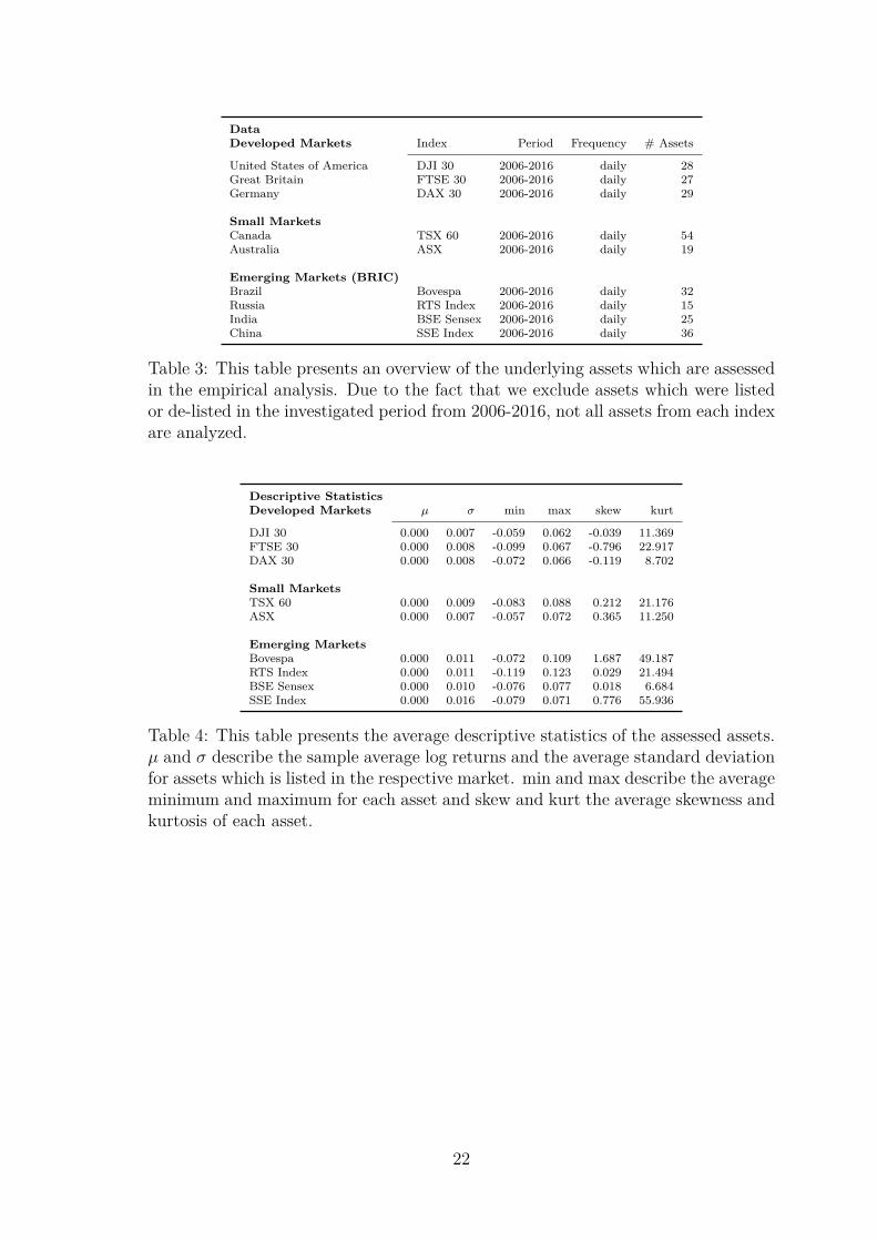
[Insert Table ?? about here.]

Table ?? presents an overview of the applied data. For all countries, we analyze

all stocks which are listed under the leading stock index of the respective coun-

try. Moreover, we exclude all stocks which were listed or de-listed after 2006 from

our analysis to ensure a consistent sample size for the assessment of different sub-

samples.

[Insert Table ?? about here.]

11This period refers to the limits of the assessed out-of-sample period and comprises up to2675 daily market quotes. Due to data intensive rolling window and wavelet analysis, the assessedmarket prices range from 6.8.2003 up to 20.5.2016 (up to 3305 observations). Due to countryspecific bank holidays, the number of observations differs marginally by each country.

15

Table ?? presents the averaged descriptive statistics of the analyzed assets for each

stock index. Obviously, the assessed stocks which are listed under indices of devel-

oped markets are characterized by lower risk (σ ranges between 0.007 and 0.008)

and extreme negative losses in comparison to positive gains (skew ranges between

-0.039 and -0.796) in comparison to stocks which are listed under indices of emerg-

ing markets, which are characterized by higher risk and a longer right tail (σ ranges

between 0.010 and 0.016; skew ranges between 0.029 and 1.687). According to the

presented averaged descriptive statistics, the investigated stocks of small markets

are characterized by similar risk as developed markets (σ ranges between 0.007 and

0.009) but by positive skewness like emerging markets (skew ranges between 0.212

and 0.365) and describe an interesting compromise between stocks of developed and

emerging markets.12.

4.2 Empirical Results

Analogous to the presented simulation analysis, we assess reconstructed return se-

ries and we start the empirical analysis by assessing the out-of-sample performance

of the portfolios that comprise stocks of developed markets. The results of the out-

of-sample performance of the global minimum variance portfolios in the period from

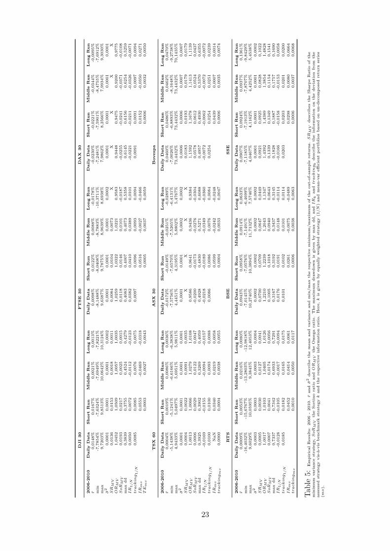
2006 until 2010 are presented in Table ??.

[Insert Table ?? about here.]

Table ?? provides the descriptive statistics and the performance metrics of the daily

out-of-sample portfolio returns from 2006 until 2010. The results for the period

between 2010 until 2016 and the crisis period from 2007 until 2009 are presented in

Table ?? and Table ?? respectively. The out-of-sample performance of the global

12As our analysis comprises 265 stocks, a detailed list of descriptive statistics for each individualasset is available upon request to the authors

16

mean-var-efficient minimum variance portfolios based on particular trends indicate,

that the decomposition of return series into different trends impacts the portfolio

performance. An exclusive focus on middle-run and long-run trends does not lead

to an improved portfolio performance in comparison to portfolios that take into

account the complete information, which is provided by the original return series.

For instance, mean-var efficient portfolio allocations which comprise stocks that are

listed under the Dow Jones index (DJI 30) lead to an average return of 0.0148%

and a Sharpe ratio of 0.0136 whereas middle-run and long-run trends leads to lower

average returns (middle run: 0.0021%; long run: 0.0013%) and lower Sharpe ratios

(middle run: 0.0018; long run: 0.0011). In contradiction to that, an exclusive focus

on short-run trends leads to marginally improved performance metrics (average out-

of-sample return: 0.0167%; Sharpe ratio 0.0153). Generally, the presented figures

suggest that daily rebalanced portfolio allocations aimed at minimizing middle-and

long-run trends of the assessed series do not improve the out-of-sample performance

in terms of the applied portfolio metrics. Turning to the assessment of short-run

trends, the results indicate that the application of decomposed short-run trends

leads to an improvement in terms of the applied quality criteria. In comparison to

the out-of-sample performance of portfolios that minimize the conditional covariance

matrix of daily data, the particular focus on short-run trends leads to higher average

returns and larger Sharpe and sortino ratios for the assessed stocks of all 9 countries.

[Insert Table ?? about here.]

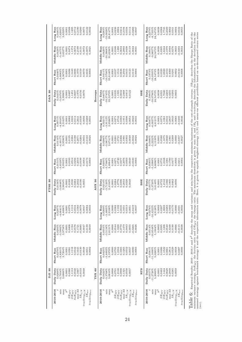
Table ?? provides the results for the time from 2010 until 2016. Although both

market times are characterized by different market regimes, i.e. the time from 2006

until 2010 includes the outbreak and the recovery of financial crisis whereas the

period between 2010 until 2016 is described by market upturns as a result of his-

torically low interest rates, the findings for the period between 2006 until 2010 hold

17

for the period 2010 until 2016. Again, by explicitly focusing on the short-run infor-

mation of the underlying daily return series, the assessed performance metrics can

be improved. Long-run information does not lead to an improvement of the applied

quality criteria. For both subsamples, extracting the short-run information from

daily return series leads to an improvement of the applied metrics, indicating that

the relevant information for applied portfolio management is adequately described

by daily short-run fluctuations.

[Insert Table ?? about here.]

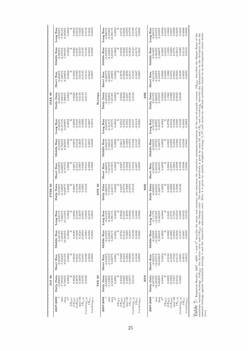
With particular focus on the market turmoil between June 2007 and June 2009, see

Table ??, portfolios that exclusively take the covariance matrix of short-run trends

into account lead to smaller negative returns (e.g. DJI 30: -0.0066% daily data and

-0.0039% short run; TSX 60: -0.0206% daily data and -0.0196% short run; RTS:

-0.0572% daily data and -0.0501% short run) than the ordinary portfolios. Again,

the results indicate that the short-run trends incorporate the relevant information

for daily portfolio management when markets are characterized by larger volatility

and collective market downturns. In this vein, the maximum drawdown in times of

market turmoil market is marginally reduced when decomposed return series that

exclusively describe the short-run trends are applied.

However, the presented results indicate that the relevant information for daily

portfolio management is adequately described by the extracted short-run informa-

tion of the respective daily return series. Therefore, exclusively focusing on the

short-run information of the assessed financial return series leads to slightly im-

proved results with respect to the assessed quality criteria. Although recent studies

mainly point at stronger dependence regimes between the long-run seasonalities of

stock returns (see Gallegati 2012, Rua and Nunes 2014, Tan et al. 2014 amongst

others), our results indicate that the information on different long-run seasonalities

18

is of limited use for applied portfolio management.

Consequently, as both middle- and long-run trends do not contribute to an im-

proved portfolio performance, our results identify the extracted information on short-

run fluctuations of the underlying return series as the relevant information for daily

portfolio management. As portfolio allocations which aim at minimizing short-run

seasonalities and classical portfolio allocations lead to comparable results, the em-

pirical findings are in line with the results of the simulation analysis and provide

evidence for the relevance of the short-run trends in the context of applied portfolio

management. Due to the applied different stock indices and sample periods, our

results are robust vis-a-vis different volatility and market regimes.

19

5 Conclusion

Triggered by the growing literature on changing dependence schemes between de-

composed return series, a simulation study and a thorough empirical assessment

reveal the relevance of short-run trends for applied portfolio management.

The presented simulation study indicates, that particular information of long-run

seasonalities is of minor relevance for daily portfolio management. Although the un-

derlying data is characterized by long-memory processes, excluding the information

of the underlying long-run seasonalities does not impact the presented portfolio allo-

cations. Moreover, the empirical assessment of different portfolios comprising stocks

which are listed on both developed and emerging markets provides evidence that

extracting short-run trends from daily return series describes the crucial information

for portfolio management.

Therefore, our results provide novel insights into the relevant information for ap-

plied portfolio management and further research should focus on the assessment of

stylized properties of the short-run trends. Moreover, alternative investment strate-

gies which take structural breaks and jumps within the short-run scales into account

or the assessment portfolio Value-at-Risk as a direct function of decomposed covari-

ance matrices present promising expansions of the presented analysis and should be

investigated.

20

6 Tables

Definition Horizon Detail

Short Run 2-4 days D1Short Run 4-8 days D2Short Run 8-16 days D3Middle Run 16-32 days D4Middle Run 32-64 days D5Long Run 64-128 days D6Long Run 128-256 days D7Long Run 256-512 days D8

Table 1: Economic interpretation of decomposed daily return series.

Original SR MR LR

d = 0.05rsim -0,0364% -0,0363% -0,0367% -0,0353%min -0,5354% -0,5346% -0,5346% -0,5502%max 0,3342% 0,3336% 0,3272% 0,3381%σsim 0,0009 0,0009 0,0009 0,0009IRmv 0,0436 -0,0349 0,0261TEmv 0,0000 0,0001 0,0004

d = 0.15rsim -0,0661% -0,0661% -0,0661% -0,0700%min -0,9148% -0,9198% -0,9062% -1,0400%max 0,7920% 0,7895% 0,7892% 0,9321%σsim 0,0022 0,0022 0,0022 0,0025IRmv 0,0024 0,0040 -0,0354TEmv 0,0001 0,0002 0,0011

d = 0.35rsim -0,1498% -0,1503% -0,1489% -0,1447%min -1,4204% -1,3997% -1,4859% -1,6412%max 1,0535% 1,0598% 1,0926% 1,4492%σsim 0,0028 0,0028 0,0029 0,0034IRmv -0,0527 0,0317 0,0330TEmv 0,0001 0,0003 0,0015

d = 0.45rsim -0,2313% -0,2316% -0,2379% -0,2368%min -10,0287% -10,0287% -10,0287% -10,7048%max 10,3812% 10,3815% 10,4105% 11,6836%σsim 0,0202 0,0203 0,0203 0,0213IRmv -0,0073 -0,0851 -0,0222TEmv 0,0004 0,0008 0,0025

Table 2: This table describes the out-of-sample results of the applied simulationstudy. rsim describes the average out-of-sample return of the mean-var efficientportfolio, min and max describe the respective minimum and maximum out-of-sample returns and σsim gives the standard deviation. IRmv describes the sum ofdeviations from the applied benchmark strategy and TEmv describes the ratio ofoverage deviation from the benchmark devided by σsim. Here, the benchmark isdefined as the portfolio based on un-decomposed data (Original).

21

DataDeveloped Markets Index Period Frequency # Assets

United States of America DJI 30 2006-2016 daily 28Great Britain FTSE 30 2006-2016 daily 27Germany DAX 30 2006-2016 daily 29

Small MarketsCanada TSX 60 2006-2016 daily 54Australia ASX 2006-2016 daily 19

Emerging Markets (BRIC)Brazil Bovespa 2006-2016 daily 32Russia RTS Index 2006-2016 daily 15India BSE Sensex 2006-2016 daily 25China SSE Index 2006-2016 daily 36

Table 3: This table presents an overview of the underlying assets which are assessedin the empirical analysis. Due to the fact that we exclude assets which were listedor de-listed in the investigated period from 2006-2016, not all assets from each indexare analyzed.

Descriptive StatisticsDeveloped Markets µ σ min max skew kurt

DJI 30 0.000 0.007 -0.059 0.062 -0.039 11.369FTSE 30 0.000 0.008 -0.099 0.067 -0.796 22.917DAX 30 0.000 0.008 -0.072 0.066 -0.119 8.702

Small MarketsTSX 60 0.000 0.009 -0.083 0.088 0.212 21.176ASX 0.000 0.007 -0.057 0.072 0.365 11.250

Emerging MarketsBovespa 0.000 0.011 -0.072 0.109 1.687 49.187RTS Index 0.000 0.011 -0.119 0.123 0.029 21.494BSE Sensex 0.000 0.010 -0.076 0.077 0.018 6.684SSE Index 0.000 0.016 -0.079 0.071 0.776 55.936

Table 4: This table presents the average descriptive statistics of the assessed assets.µ and σ describe the sample average log returns and the average standard deviationfor assets which is listed in the respective market. min and max describe the averageminimum and maximum for each asset and skew and kurt the average skewness andkurtosis of each asset.

22

DJ

I3

0F

TS

E3

0D

AX

30

20

06

-20

10

Dai

lyD

ata

Sh

ort

Ru

nM

idd

leR

un

Lo

ng

Ru

nD

aily

Dat

aS

ho

rtR

un

Mid

dle

Ru

nL

on

gR

un

Dai

lyD

ata

Sh

ort

Ru

nM

idd

leR

un

Lo

ng

Ru

nr

0,01

48%

0,01

67%

0,00

21%

0,00

13%

0,00

98%

0,01

22%

0,00

88%

-0,0

178%

-0,0

230%

-0,0

221%

-0,0

344%

-0,0

095%

min

-7,7

854%

-7,6

324%

-7,6

949%

-7,8

221%

-8,1

488%

-8,0

408%

-8,7

883%

-10,

3711

%-7

,248

1%-7

,590

1%-8

,475

5%-7

,691

2%m

ax9,

7203

%9,

8513

%10

,064

2%10

,312

4%9,

6387

%9,

7875

%8,

9639

%8,

6938

%7,

9862

%8,

2566

%7,

9934

%9,

3030

%σ

20,

0001

0,00

010,

0001

0,00

020,

0001

0,00

010,

0001

0,00

020,

0001

0,00

010,

0001

0,00

01SR

MV

0,01

360,

0153

0,00

180,

0011

0,00

840,

0104

0,00

73X

XX

XX

OR

MV

1,04

521,

0509

1,00

571,

0035

1,02

591,

0322

1,02

210,

9583

0,94

480,

9475

0,92

000,

9775

SoR

MV

0,01

930,

0217

0,00

250,

0015

0,01

180,

0146

0,01

01-0

,018

7-0

,025

5-0

,024

1-0

,037

1-0

,010

8m

axdd

0,38

390,

3755

0,45

240,

4279

0,40

830,

4007

0,40

730,

5358

0,61

450,

6156

0,62

540,

5259

IR

1/N

0,00

500,

0072

-0,0

112

-0,0

123

0,03

820,

0410

0,03

890,

0101

-0,0

221

-0,0

211

-0,0

326

-0,0

071

tracking

1/N

0,00

850,

0085

0,00

760,

0075

0,00

970,

0096

0,00

930,

0094

0,00

910,

0091

0,00

970,

0094

IR

mv

0,05

53-0

,046

9-0

,031

80,

0516

-0,0

027

-0,0

466

0,01

52-0

,035

00,

0271

TE

mv

0,00

030,

0027

0,00

430,

0005

0,00

370,

0059

0,00

060,

0032

0,00

50

TS

X6

0A

SX

30

Bov

esp

a

20

06

-20

10

Dai

lyD

ata

Sh

ort

Ru

nM

idd

leR

un

Lo

ng

Ru

nD

aily

Dat

aS

ho

rtR

un

Mid

dle

Ru

nL

on

gR

un

Dai

lyD

ata

Sh

ort

Ru

nM

idd

leR

un

Lo

ng

Ru

nr

0,00

04%

0,00

19%

0,00

86%

0,00

36%

-0,0

172%

-0,0

149%

-0,0

251%

-0,0

289%

0,04

60%

0,04

86%

0,04

62%

0,04

70%

min

-5,1

438%

-5,1

241%

-6,6

166%

-6,3

838%

-7,5

756%

-7,6

570%

-7,5

265%

-6,4

131%

-7,0

026%

-6,8

893%

-8,1

648%

-9,2

738%

max

4,94

33%

5,04

97%

5,69

51%

5,98

11%

4,44

51%

4,31

95%

5,88

02%

5,47

67%

73,4

432%

73,4

432%

73,4

432%

70,1

435%

σ2

0,00

010,

0001

0,00

010,

0001

0,00

010,

0001

0,00

020,

0002

0,00

060,

0006

0,00

070,

0007

SR

MV

0,00

040,

0022

0,00

910,

0035

XX

XX

0,01

830,

0193

0,01

790,

0179

OR

MV

1,00

131,

0066

1,02

791,

0108

0,95

860,

9641

0,94

360,

9384

1,15

921,

1678

1,14

131,

1139

SoR

MV

0,00

060,

0029

0,01

220,

0047

-0,0

200

-0,0

173

-0,0

276

-0,0

304

0,05

780,

0612

0,05

240,

0437

max

dd0,

3925

0,39

020,

3269

0,40

590,

4928

0,48

300,

5271

0,60

880,

4957

0,49

300,

5370

0,63

55IR

1/N

-0,0

169

-0,0

155

-0,0

094

-0,0

157

-0,0

218

-0,0

189

-0,0

349

-0,0

360

-0,0

072

-0,0

062

-0,0

072

-0,0

072

tracking

1/N

0,01

000,

0100

0,00

930,

0088

0,00

860,

0086

0,00

760,

0084

0,02

540,

0254

0,02

510,

0239

IR

mv

NaN

0,03

400,

0219

0,00

580,

0599

-0,0

242

-0,0

248

0,04

390,

0007

0,00

14tracking

mv

0,00

000,

0004

0,00

380,

0055

0,00

040,

0033

0,00

470,

0006

0,00

350,

0074

RT

SB

SE

SS

E

20

06

-20

10

Dai

lyD

ata

Sh

ort

Ru

nM

idd

leR

un

Lo

ng

Ru

nD

aily

Dat

aS

ho

rtR

un

Mid

dle

Ru

nL

on

gR

un

Dai

lyD

ata

Sh

ort

Ru

nM

idd

leR

un

Lo

ng

Ru

nr

0,00

09%

0,00

53%

0,02

16%

0,00

80%

0,09

43%

0,09

58%

0,09

14%

0,06

33%

0,09

07%

0,09

24%

0,09

37%

0,13

61%

min

-16,

4032

%-1

5,67

67%

-13,

2803

%-1

2,98

18%

-7,0

145%

-7,0

576%

-7,1

491%

-6,4

699%

-7,1

185%

-7,1

913%

-7,8

707%

-9,8

429%

max

9,60

29%

10,0

595%

9,38

45%

12,4

053%

10,2

740%

10,3

894%

11,7

132%

7,57

46%

4,04

67%

4,11

62%

4,42

52%

5,45

38%

σ2

0,00

030,

0003

0,00

030,

0004

0,00

020,

0002

0,00

020,

0002

0,00

010,

0001

0,00

010,

0002

SR

MV

0,00

050,

0030

0,01

270,

0041

0,07

000,

0709

0,06

470,

0449

0,09

210,

0925

0,08

280,

1022

OR

MV

1,00

171,

0103

1,04

051,

0126

1,22

101,

2239

1,20

431,

1347

1,43

921,

4389

1,38

541,

4828

SoR

MV

0,00

070,

0041

0,01

740,

0056

0,10

050,

1018

0,09

400,

0643

0,13

390,

1349

0,11

540,

1541

max

dd0,

7337

0,73

420,

6933

0,72

910,

3167

0,31

920,

3437

0,31

450,

1828

0,18

870,

1757

0,16

90IR

1/N

-0,0

128

-0,0

105

-0,0

017

-0,0

094

0,01

760,

0191

0,01

48-0

,011

4-0

,016

6-0

,015

8-0

,015

30,

0058

tracking

1/N

0,01

850,

0182

0,01

650,

0175

0,01

010,

0102

0,01

010,

0114

0,02

030,

0203

0,02

010,

0200

IR

mv

0,04

520,

0414

0,00

610,

0261

-0,0

075

-0,0

489

0,02

980,

0080

0,06

64tracking

mv

0,00

100,

0050

0,01

170,

0006

0,00

380,

0063

0,00

060,

0037

0,00

68

Tabl

e5:

Em

piri

cal

Res

ults

:20

06-

2010

.r

andσ

2de

scri

be

the

mea

nan

dva

rian

cean

dm

in/m

axth

ere

spec

tive

min

imum

/max

imum

ofth

eou

t-of

-sam

ple

retu

rns.SR

MV

desc

rib

esth

eSh

arp

eR

atio

ofth

em

inim

umva

rian

cest

rate

gy,SoR

MV

the

Sort

ino

rati

oan

dOR

MV

the

Om

ega

rati

o.T

hem

axim

umdr

awdo

wn

isgi

ven

bym

axdd

,an

dIR

kan

dtracking

kde

scri

be

the

info

rmat

ion

onth

ede

viat

ion

from

the

asse

ssed

stra

tegy

vis-

a-vi

sb

ench

mar

kst

rate

gyk

and

the

resp

ecti

vein

form

atio

nra

tio.

Her

e,k

isgi

ven

byeq

ually

wei

ghte

dst

rate

gy(1/N

)an

dm

ean-

var

effici

ent

por

tfol

ios

base

don

un-d

ecom

pos

edre

turn

seri

es(mv).

23

DJ

I3

0F

TS

E3

0D

AX

30

20

10

-20

16

Dai

lyD

ata

Sh

ort

Ru

nM

idd

leR

un

Lo

ng

Ru

nD

aily

Dat

aS

ho

rtR

un

Mid

dle

Ru

nL

on

gR

un

Dai

lyD

ata

Sh

ort

Ru

nM

idd

leR

un

Lo

ng

Ru

nr

0,02

69%

0,02

70%

0,02

93%

0,02

97%

0,01

56%

0,01

51%

0,01

16%

0,00

71%

0,04

45%

0,04

46%

0,04

29%

0,04

85%

min

-3,7

954%

-3,8

201%

-3,5

992%

-4,0

641%

-3,6

648%

-3,6

529%

-4,4

917%

-4,2

918%

-5,6

470%

-5,6

082%

-5,4

475%

-7,6

292%

max

3,68

66%

3,72

04%

3,97

58%

4,44

96%

3,96

54%

3,95

03%

3,95

96%

3,51

62%

3,39

96%

3,36

70%

3,63

37%

3,62

29%

σ2

0,00

010,

0001

0,00

010,

0001

0,00

010,

0001

0,00

010,

0001

0,00

010,

0001

0,00

010,

0001

SR

MV

0,03

800,

0381

0,04

060,

0379

0,01

890,

0183

0,01

350,

0082

0,04

970,

0496

0,04

740,

0508

OR

MV

1,11

131,

1118

1,11

941,

1113

1,05

301,

0514

1,03

841,

0224

1,14

511,

1449

1,13

741,

1495

SoR

MV

0,05

400,

0542

0,05

760,

0534

0,02

640,

0256

0,01

880,

0114

0,06

970,

0696

0,06

720,

0712

max

dd0,

1667

0,16

450,

1721

0,15

830,

2032

0,20

190,

2071

0,26

410,

1970

0,19

700,

2199

0,21

90IR

1/N

-0,0

133

-0,0

130

-0,0

085

-0,0

078

-0,0

190

-0,0

199

-0,0

264

-0,0

339

0,01

560,

0159

0,01

310,

0200

tracking

1/N

0,00

480,

0048

0,00

470,

0047

0,00

550,

0054

0,00

540,

0056

0,00

700,

0070

0,00

720,

0075

IR

mv

0,00

510,

0139

0,00

84-0

,017

3-0

,016

3-0

,026

90,

0035

-0,0

075

0,01

22tracking

mv

0,00

020,

0018

0,00

330,

0003

0,00

240,

0031

0,00

030,

0021

0,00

32

TS

X6

0A

SX

30

Bov

esp

a

20

10

-20

16

Dai

lyD

ata

Sh

ort

Ru

nM

idd

leR

un

Lo

ng

Ru

nD

aily

Dat

aS

ho

rtR

un

Mid

dle

Ru

nL

on

gR

un

Dai

lyD

ata

Sh

ort

Ru

nM

idd

leR

un

Lo

ng

Ru

nr

0,04

22%

0,04

25%

0,03

53%

0,02

69%

0,02

14%

0,02

05%

0,02

06%

0,02

21%

0,04

07%

0,04

11%

0,04

20%

0,02

83%

min

-3,3

768%

-3,4

492%

-3,5

134%

-3,4

805%

-3,7

120%

-3,7

566%

-3,9

817%

-3,9

112%

-10,

5745

%-1

0,57

00%

-10,

3868

%-1

0,00

28%

max

3,08

10%

3,19

70%

2,81

31%

2,91

08%

2,41

04%

2,40

64%

2,67

41%

2,65

86%

33,5

379%

33,6

140%

31,6

236%

28,8

147%

σ2

0,00

000,

0000

0,00

000,

0000

0,00

010,

0001

0,00

010,

0001

0,00

010,

0001

0,00

010,

0001

SR

MV

0,07

010,

0705

0,05

440,

0382

0,02

840,

0271

0,02

610,

0271

0,03

350,

0337

0,03

480,

0236

OR

MV

1,21

461,

2164

1,16

001,

1102

1,07

761,

0740

1,07

211,

0744

1,15

051,

1514

1,14

881,

0904

SoR

MV

0,09

980,

1005

0,07

700,

0535

0,03

960,

0377

0,03

660,

0383

0,06

320,

0636

0,06

340,

0414

max

dd0,

1321

0,12

650,

1479

0,16

510,

2033

0,20

760,

1991

0,19

110,

2468

0,25

040,

2893

0,21

94IR

1/N

0,05

500,

0552

0,04

430,

0313

0,03

200,

0303

0,03

030,

0306

0,04

130,

0415

0,04

380,

0334

tracking

1/N

0,00

570,

0057

0,00

550,

0051

0,00

490,

0049

0,00

490,

0054

0,01

220,

0123

0,01

190,

0114

IR

mv

0,00

90-0

,026

5-0

,041

9-0

,033

0-0

,003

20,

0023

0,01

100,

0044

-0,0

266

tracking

mv

0,00

030,

0026

0,00

370,

0003

0,00

240,

0031

0,00

040,

0031

0,00

47

RT

SB

SE

SS

E

20

10

-20

16

Dai

lyD

ata

Sh

ort

Ru

nM

idd

leR

un

Lo

ng

Ru

nD

aily

Dat

aS

ho

rtR

un

Mid

dle

Ru

nL

on

gR

un

Dai

lyD

ata

Sh

ort

Ru

nM

idd

leR

un

Lo

ng

Ru

nr

0,05

57%

0,05

81%

0,05

14%

0,02

76%

0,05

77%

0,05

85%

0,04

80%

0,03

47%

0,19

84%

0,19

73%

0,18

84%

0,22

79%

min

-11,

2726

%-1

1,16

90%

-10,

8548

%-1

0,42

22%

-5,3

720%

-5,3

388%

-5,2

222%

-6,0

037%

-10,

0796

%-1

0,05

05%

-9,9

857%

-8,7

335%

max

5,20

00%

5,02

85%

5,19

04%

4,91

26%

3,61

49%

3,66

96%

4,11

39%

4,61

21%

24,5

473%

24,5

473%

24,5

473%

24,5

473%

σ2

0,00

010,

0001

0,00

020,

0002

0,00

010,

0001

0,00

010,

0001

0,00

380,

0038

0,00

380,

0038

SR

MV

0,04

620,

0486

0,03

950,

0207

0,07

220,

0731

0,05

800,

0374

0,03

210,

0320

0,03

050,

0368

OR

MV

1,14

441,

1522

1,12

061,

0603

1,21

421,

2168

1,16

751,

1061

1,70

401,

6920

1,62

441,

7745

SoR

MV

0,06

290,

0661

0,05

400,

0283

0,10

660,

1081

0,08

400,

0531

0,22

030,

2153

0,19

790,

2509

max

dd0,

2848

0,28

140,

3248

0,34

020,

1805

0,17

800,

1961

0,28

370,

4255

0,43

600,

4944

0,46

62IR

1/N

0,02

850,

0329

0,01

90-0

,017

00,

0462

0,04

770,

0269

0,00

430,

0293

0,02

910,

0276

0,03

41tracking

1/N

0,00

590,

0058

0,00

660,

0066

0,00

560,

0056

0,00

600,

0065

0,06

030,

0602

0,06

030,

0604

IR

mv

0,03

87-0

,011

5-0

,050

10,

0211

-0,0

357

-0,0

495

-0,0

133

-0,0

293

0,05

32tracking

mv

0,00

060,

0038

0,00

560,

0004

0,00

270,

0046

0,00

080,

0034

0,00

55

Tabl

e6:

Em

piri

cal

Res

ults

:20

10-

2016.r

andσ

2de

scri

be

the

mea

nan

dva

rian

cean

dm

in/m

axth

ere

spec

tive

min

imum

/max

imum

ofth

eou

t-of

-sam

ple

retu

rns.SR

MV

desc

rib

esth

eSh

arp

eR

atio

ofth

em

inim

umva

rian

cest

rate

gy,SoR

MV

the

Sort

ino

rati

oan

dOR

MV

the

Om

ega

rati

o.T

hem

axim

umdr

awdo

wn

isgi

ven

bym

axdd

,an

dIR

kan

dtracking

kde

scri

be

the

info

rmat

ion

onth

ede

viat

ion

from

the

asse

ssed

stra

tegy

agai

nst

ben

chm

ark

stra

tegy

kan

dth

ere

spec

tive

info

rmat

ion

rati

o.H

ere,k

isgi

ven

byeq

ually

wei

ghte

dst

rate

gy(1/N

)an

dm

ean-

var

effici

ent

por

tfol

ios

base

don

un-d

ecom

pos

edre

turn

seri

es(mv).

24

DJ

I3

0F

TS

E3

0D

AX

30

20

07

-20

09

Dai

lyD

ata

Sh

ort

Ru

nM

idd

leR

un

Lo

ng

Ru

nD

aily

Dat

aS

ho

rtR

un

Mid

dle

Ru

nL

on

gR

un

Dai

lyD

ata

Sh

ort

Ru

nM

idd

leR

un

Lo

ng

Ru

nr

-0,0

066%

-0,0

039%

-0,0

214%

-0,0

211%

-0,0

192%

-0,0

160%

-0,0

168%

-0,0

642%

-0,0

843%

-0,0

846%

-0,0

856%

-0,0

580%

min

-7,7

854%

-7,6

324%

-7,6

949%

-7,8

221%

-8,1

488%

-8,0

408%

-8,7

883%

-10,

3711

%-7

,248

1%-7

,590

1%-8

,475

5%-7

,691

2%m

ax9,

7203

%9,

8513

%10

,064

2%10

,312

4%9,

6387

%9,

7875

%8,

9639

%8,

6938

%7,

9862

%8,

2566

%7,

9934

%9,

3030

%σ

20,

0002

0,00

020,

0002

0,00

020,

0002

0,00

020,

0002

0,00

020,

0002

0,00

020,

0002

0,00

02SR

MV

XX

XX

XX

XX

XX

XX

OR

MV

0,98

480,

9910

0,95

600,

9582

0,96

070,

9671

0,96

760,

8856

0,83

390,

8352

0,83

460,

8853

SoR

MV

-0,0

070

-0,0

041

-0,0

206

-0,0

194

-0,0

188

-0,0

157

-0,0

158

-0,0

545

-0,0

799

-0,0

789

-0,0

791

-0,0

578

max

dd0,

3839

0,37

550,

4524

0,42

790,

4024

0,39

570,

4027

0,53

010,

6145

0,61

560,

6254

0,52

25IR

1/N

0,01

350,

0161

-0,0

004

-0,0

001

0,04

630,

0493

0,05

100,

0098

-0,0

142

-0,0

145

-0,0

145

0,00

87tracking

1/N

0,01

060,

0106

0,00

940,

0092

0,01

220,

0121

0,01

150,

0116

0,01

130,

0113

0,01

200,

0116

IR

mv

0,06

56-0

,045

6-0

,027

90,

0569

0,00

53-0

,060

7-0

,004

3-0

,003

40,

0445

tracking

mv

0,00

040,

0033

0,00

520,

0006

0,00

460,

0074

0,00

070,

0038

0,00

59

TS

X6

0A

SX

30

Bov

esp

a

20

07

-20

09

Dai

lyD

ata

Sh

ort

Ru

nM

idd

leR

un

Lo

ng

Ru

nD

aily

Dat

aS

ho

rtR

un

Mid

dle

Ru

nL

on

gR

un

Dai

lyD

ata

Sh

ort

Ru

nM

idd

leR

un

Lo

ng

Ru

nr

-0,0

206%

-0,0

196%

-0,0

103%

-0,0

153%

-0,0

905%

-0,0

865%

-0,0

841%

-0,0

979%

-0,0

656%

-0,0

627%

-0,0

725%

-0,0

801%

min

-5,1

438%

-5,1

241%

-6,6

166%

-6,3

838%

-7,5

756%

-7,6

570%

-7,5

265%

-6,4

131%

-7,0

026%

-6,8

893%

-8,1

648%

-9,2

738%

max

4,94

33%

5,04

97%

5,69

51%

5,98

11%

4,44

51%

4,31

95%

5,88

02%

5,47

67%

7,29

18%

7,49

88%

8,05

35%

12,9

811%

σ2

0,00

010,

0001

0,00

010,

0002

0,00

020,

0002

0,00

030,

0003

0,00

020,

0002

0,00

020,

0003

SR

MV

XX

XX

XX

XX

XX

XX

OR

MV

0,94

350,

9468

0,97

340,

9640

0,84

370,

8507

0,86

110,

8515

0,85

040,

8570

0,85

390,

8721

SoR

MV

-0,0

267

-0,0

253

-0,0

121

-0,0

167

-0,0

770

-0,0

734

-0,0

687

-0,0

765

-0,0

649

-0,0

622

-0,0

648

-0,0

586

max

dd0,

3925

0,39

020,

3269

0,40

590,

3098

0,30

280,

3384

0,39

410,

4957

0,49

300,

5370

0,63

55IR

1/N

-0,0

077

-0,0

069

0,00

10-0

,003

8-0

,037

9-0

,034

7-0

,037

5-0

,044

9-0

,053

0-0

,051

1-0

,062

8-0

,077

8tracking

1/N

0,01

190,

0118

0,01

080,

0100

0,01

430,

0145

0,01

280,

0137

0,01

330,

0133

0,01

240,

0109

IR

mv

0,01

920,

0228

0,00

800,

0857

0,01

47-0

,011

30,

0407

-0,0

170

-0,0

174

tracking

mv

0,00

050,

0045

0,00

660,

0005

0,00

430,

0065

0,00

070,

0041

0,00

84

RT

SB

SE

SS

E

20

07

-20

09

Dai

lyD

ata

Sh

ort

Ru

nM

idd

leR

un

Lo

ng

Ru

nD

aily

Dat

aS

ho

rtR

un

Mid

dle

Ru

nL

on

gR

un

Dai

lyD

ata

Sh

ort

Ru

nM

idd

leR

un

Lo

ng

Ru

nr

-0,0

572%

-0,0

501%

-0,0

358%

-0,1

117%

-0,0

090%

-0,0

075%

-0,0

234%

-0,0

112%

0,01

15%

0,01

16%

0,01

36%

0,00

91%

min

-16,

4032

%-1

5,67

67%

-13,

2803

%-1

2,98

18%

-6,6

434%

-6,5

910%

-7,1

072%

-6,4

699%

-2,2

669%

-2,3

230%

-2,3

643%

-2,9

543%

max

9,60

29%

10,0

595%

9,38

45%

12,4

053%

5,43

87%

5,40

12%

5,12

87%

5,30

15%

2,37

24%

2,41

63%

2,34

60%

3,32

40%

σ2

0,00

040,

0004

0,00

030,

0004

0,00

020,

0002

0,00

020,

0002

0,00

000,

0000

0,00

000,

0000

SR

MV

XX

XX

XX

XX

0,03

340,

0325

0,03

160,

0167

OR

MV

0,90

050,

9124

0,93

920,

8421

0,98

230,

9854

0,95

810,

9798

1,19

621,

1886

1,16

831,

0840

SoR

MV

-0,0

383

-0,0

335

-0,0

260

-0,0

731

-0,0

086

-0,0

071

-0,0

209

-0,0

102

0,04

860,

0472

0,04

690,

0257

max

dd0,

7337

0,73

420,

6933

0,72

910,

2959

0,29

630,

3356

0,31

000,

0559

0,05

640,

0770

0,09

98IR

1/N

-0,0

144

-0,0

115

-0,0

056

-0,0

416

0,05

860,

0598

0,04

820,

0560

-0,0

022

-0,0

022

-0,0

014

-0,0

033

tracking

1/N

0,02

250,

0221

0,01

970,

0209

0,01

260,

0126

0,01

240,

0128

0,02

480,

0248

0,02

460,

0242

IR

mv

0,06

130,

0361

-0,0

442

0,02

48-0

,034

9-0

,003

50,

0024

0,01

10-0

,008

8tracking

mv

0,00

120,

0059

0,01

230,

0006

0,00

410,

0062

0,00

020,

0019

0,00

28

Tabl

e7:

Em

piri

cal

Res

ults

:20

07-

2009

.r

andσ

2de

scri

be

the

mea

nan

dva

rian

cean

dm

in/m

axth

ere

spec

tive

min

imum

/max

imum

ofth

eou

t-of

-sam

ple

retu

rns.SR

MV

desc

rib

esth

eSh

arp

eR

atio

ofth

em

inim

umva

rian

cest

rate

gy,SoR

MV

the

Sort

ino

rati

oan

dOR

MV

the

Om

ega

rati

o.T

hem

axim

umdr

awdo

wn

isgi

ven

bym

axdd

,an

dIR

kan

dtracking

kde

scri

be

the

info

rmat

ion

onth

ede

viat

ion

from

the

asse

ssed

stra

tegy

agai

nst

ben

chm

ark

stra

tegy

kan

dth

ere

spec

tive

info

rmat

ion

rati

o.H

ere,k

isgi

ven

byeq

ually

wei

ghte

dst

rate

gy(1/N

)an

dm

ean-

var

effici

ent

por

tfol

ios

base

don

un-d

ecom

pos

edre

turn

seri

es(mv).

25

References

[1] Andries, A. M., Ihnatov, I., Tiwari, A. K., 2014. Analyzing time frequency rela-

tionship between interest rate, stock price and exchange rate through continuous

wavelet. Economic Modelling, 41(1), 227-238.

[2] Ane, T., Kharoubi, C., 2003. Dependence structure and risk measure. Journal of

Business, 76 (3), 411Ű438.

[3] Berger, T., 2016. On the isolated impact of copulas on risk measurement: A

simulation study. Economic Modelling, 58 (1), 475-481.

[4] Berger, T., Uddin, G.L., 2016. On the dynamic dependence between equity mar-

kets, commodity futures and economic uncertainty indexes. Energy Economics,

56(1), 374-383.

[5] Berger, T., Gencay, R, 2016. Long run trends and Value-at-Risk forecasts. work-

ing paper.

[6] Baillie, R.T., Bollerslev, T., Mikkelsen, H.O., 1996. Fractionally integrated gen-

eralized autoregressive conditional heteroskedasticity, Journal of Econometrics,

74(1), 3-30.

[7] Baillie, R.T., Morana C., 2009. Modeling long memory and structural breaks in

conditional variances: An adaptive FIGARCH approach, Journal of Economic

Dynamics and Control, 33(8), 1577-1592.

[8] Bollerslev, T., 1986. Generalized Autoregressive Conditional Heteroskedasticity,

Journal of Econometrics, 31(3), 307-327.

[9] Boubaker, H., Sghaier, L., 2013. Portfolio optimization in the presence of depen-

dent financial returns with long memory: A copula based approach. Journal of

Banking and Finance, 37(1), 361-377.

26

[10] Crowley, P.M., 2007. A guide to wavelets for economists, Journal of Economic

Surveys, 21(1), 207-267.

[11] De Miguel V., Garlappi L., Uppal R., 2009. Optimal versus naive diversification:

How inefficient is the 1/n portfolio strategy. Review of financial studies, 22 (1),

1915-1953.

[12] Dewandaru, G., Masih, R., Masih, A.M.M., 2015. Why is no financial crisis a

dress rehearsal for the next? Exploring contagious heterogeneities across major

Asian stock markets. Physica A, 419(1), 241-259.

[13] Engle, R., (2002). Dynamic conditional correlation: A simple class of multi-

variate generalized autoregressive conditional heteroscedasticity models, Journal

of Business and Economic Statistics, 20 (3), 339-350.

[14] Engle, R., (2009). Anticipating correlations: A new paradigm for risk manage-

ment, Princeton University Press.

[15] Fantazzini, D., 2009. The effects of misspecified marginals and copulas on com-

puting value at risk: a monte carlo study. Computational Statistics and Data

Analysis, 53 (6), 2168-2188.

[16] Gallegati, M., 2012. A wavelet-based approach to test for financial market con-

tagion. Computational Statistics and Data Analysis, 56, 3491-3497.

[17] Gencay, R., Selcuk, F., Whitcher, B., 2001. An introduction to wavelets and

other filtering methods in finance and economics. Academic Press: San Diego.

[18] Gencay, R., Selcuk, F., Whitcher, B., 2003. Systematic risk and timescales.

Quantitative Finance, 3 (2), 108-116.

[19] Gencay, R., Selcuk, F., Whitcher, B., 2005. Multiscale systematic risk. Journal

of International Money and Finance, 24 (1), 55-70.

[20] Markowitz, H., 1952. Portfolio selection. The Journal of Finance, 7 (1), 77-91.

27

[21] O’Neil, J., 2001. Building better global econimc BRICs, Goldman Sachs Global

Economics Paper, 66 (1).

[22] Percival, D. B., Walden, A., 2000. Wavelet methods for time series analysis,

Cambridge University Press.

[23] Reboredo, J., Rivera-Castro, M., 2014. Wavelet-based evidence of the impact of

oil prices on stock returns. International Review of Economics and Finance, 29,

145-176.

[24] Grinold, R.C., Kahn, R.N., 2000. Active Portfolio Management, 2nd. ed.,

McGraw-Hill.

[25] Rua, A., Nunes, L. C., 2014. A wavelet-based assessment of market risk: The

emerging market case. The Quarterly Review of Economics and Finance, 52,

84-92.

[26] Shadwick, W.F., Keating. C., (2002). A universal performance measure. Journal

of performance Measurement, 4, 59-84.

[27] Sortino, F.A., van der Meer, R., (1991). Downside risk. The journal of portfolio

management, 4, 27-31.

[28] Sun, E. W., Chen, Y.T., Yu, M.T., 2015. Generalized optimal wavelet decom-

position algorithm for big financial data. International Journal of Production

Economics, 165, 194-214.

[29] Tan, P.P., Chin, C.W., Galagedera, D.U.A., 2014. A wavelet-based evaluation

of time-varying long memory of equity markets: A paradigm in crisis. Physica

A, 410, 345-358.

[30] Zhu, L., Wang, Y., Fan, Q., 2014. MODWT-ARMA model for time series pre-

diction. Applied Mathematical Modelling, 38, 1859-1865.

28