extractive institutions in colonial africa - caltechthesis · extractive institutions in colonial...
TRANSCRIPT

Extractive Institutions in Colonial Africa
Thesis by
Federico Tadei
In Partial Fulfillment of the Requirements
for the Degree of
Doctor of Philosophy
California Institute of Technology
Pasadena, California
2014
(Defended May 16, 2014)

ii
c© 2014
Federico Tadei
All Rights Reserved

iii
Ai miei genitori, Anna Maria e Roberto, e a mio fratello, Alessandro

iv
Acknowledgments
I would like to thank the faculty, students, and staff of the Division of Humanities
and Social Sciences at the California Institute of Technology for providing me with
a productive and enjoyable research environment. I am deeply indebted to my advi-
sor, Jean-Laurent Rosenthal, for his excellent guidance and encouragement, and for
teaching me what it means being an economic historian. For stimulating conversa-
tions and helpful comments, I am also grateful to Jean Ensminger, Philip Hoffman,
Erik Snowberg, Matt Shum, and the participants to the Caltech HSS Proseminar,
Social Science-History Lunch, and All-UC Economic History Group. I would like to
thank the staff of the French National Library in Paris and the colonial archives in
Aix-en-Provence, for assistance with data collection, and the HSS Division at Caltech,
for providing the funding which made it possible. I also want to thank Maristella Bot-
ticini, who introduced me first to economic history. Many good friends, in the United
States and in Italy, helped me with their support and friendship. Special thanks
go to my roomate Britton and to Alberto, Bill, Blandine, Bose, Chiara, Daniele,
Emilia, Giada, Giulia C., Giulia F., Nacho, Sirio, and Stefano. Finally, Brenda, my
aunt Anna, my brother Alessandro, and my parents, Anna Maria and Roberto, each
provided extraordinary example, encouragement, and love.
v
Abstract
A common explanation for African current underdevelopment is the extractive charac-
ter of institutions established during the colonial period. Yet, since colonial extraction
is hard to quantify and its exact mechanisms are not well understood, we still do not
know precisely how colonial institutions affect economic growth today. In this project,
I study this issue by focusing on the peculiar structure of trade and labor policies
employed by the French colonizers.
First, I analyze how trade monopsonies and coercive labor institutions reduced
African gains from trade during the colonial period. By using new data on prices to
agricultural producers and labor institutions in French Africa, I show that (1) the
monopsonistic character of colonial trade implied a reduction in prices to producers
far below world market prices; (2) coercive labor institutions allowed the colonizers
to reduce prices even further; (3) as a consequence, colonial extraction cut African
gains from trade by over 60%.
Given the importance of labor institutions, I then focus on their origin by analyz-
ing the colonial governments’ incentives to choose between coerced and free labor. I
argue that the choice of institutions was affected more by the properties of exported
commodities, such as prices and economies of scale, than by the characteristics of
colonies, such indigenous population density and ease of settlement for the coloniz-
ers.
Finally, I study the long-term effects of colonial trade monopsonies and coercive

vi
labor institutions. By combining archival data on prices in the French colonies with
maps of crop suitability, I show that the extent to which prices to agricultural produc-
ers were reduced with respect to world market prices is strongly negatively correlated
with current regional development, as proxied by luminosity data from satellite im-
ages. The evidence suggests that colonial extraction affected subsequent growth by
reducing development in rural areas in favor of a urban elite. The differential impact
in rural and urban areas can be the reason why trade monopsonies and extractive
institutions persisted long after independence.
vii
Contents
Acknowledgments iv
Abstract v
1 Introduction 1
2 Extractive Institutions and Gains From Trade: Evidence from Colo-
nial Africa 6
2.1 Introduction . . . . . . . . . . . . . . . . . . . . . . . . . . . . . . . . 6
2.2 Historical Background . . . . . . . . . . . . . . . . . . . . . . . . . . 9
2.3 A Model of Colonial Extraction . . . . . . . . . . . . . . . . . . . . . 16
2.4 Result 1: Prices to Africans and Competitive Prices . . . . . . . . . . 19
2.4.1 Data . . . . . . . . . . . . . . . . . . . . . . . . . . . . . . . . 19
2.4.2 Empirical Strategy . . . . . . . . . . . . . . . . . . . . . . . . 22
2.4.3 Results . . . . . . . . . . . . . . . . . . . . . . . . . . . . . . . 26
2.5 Result 2: Labor Institutions and Prices to Africans . . . . . . . . . . 31
2.6 Result 3: Colonial Extraction and Gains from Trade . . . . . . . . . . 37
2.7 Conclusion . . . . . . . . . . . . . . . . . . . . . . . . . . . . . . . . . 41
2.8 Appendix . . . . . . . . . . . . . . . . . . . . . . . . . . . . . . . . . 42
2.8.1 Prices in France and World Market Prices . . . . . . . . . . . 42
2.8.2 Post-Independence Prices . . . . . . . . . . . . . . . . . . . . 43

viii
2.8.3 Data Sources . . . . . . . . . . . . . . . . . . . . . . . . . . . 44
2.8.4 Appendix Figures and Tables . . . . . . . . . . . . . . . . . . 46
3 The Origins of Extractive Institutions: Labor in Colonial French
Africa 48
3.1 Introduction . . . . . . . . . . . . . . . . . . . . . . . . . . . . . . . . 48
3.2 Historical Background and Data . . . . . . . . . . . . . . . . . . . . . 51
3.3 Crops or Locations? . . . . . . . . . . . . . . . . . . . . . . . . . . . . 53
3.3.1 Preliminary Analysis . . . . . . . . . . . . . . . . . . . . . . . 53
3.3.2 Empirical Analysis . . . . . . . . . . . . . . . . . . . . . . . . 55
3.4 What is Behind Crop Fixed Effects? . . . . . . . . . . . . . . . . . . 60
3.4.1 Theoretical Framework . . . . . . . . . . . . . . . . . . . . . . 61
3.4.2 Testable Implications and Evidence . . . . . . . . . . . . . . . 66
3.5 Conclusion . . . . . . . . . . . . . . . . . . . . . . . . . . . . . . . . . 67
3.6 Appendix . . . . . . . . . . . . . . . . . . . . . . . . . . . . . . . . . 69
3.6.1 Definition and Sources . . . . . . . . . . . . . . . . . . . . . . 69
3.6.2 Appendix Figures and Tables . . . . . . . . . . . . . . . . . . 69
4 Colonial Institutions, Prices to Producers, and Current African De-
velopment 71
4.1 Introduction . . . . . . . . . . . . . . . . . . . . . . . . . . . . . . . . 71
4.2 Historical Background and Data . . . . . . . . . . . . . . . . . . . . . 73
4.2.1 Price Gaps . . . . . . . . . . . . . . . . . . . . . . . . . . . . . 74
4.2.2 Luminosity . . . . . . . . . . . . . . . . . . . . . . . . . . . . 77
4.3 Colonial Price Gaps and Current Development . . . . . . . . . . . . . 78
4.4 Channels of Causality: Effects on Rural and Urban Areas . . . . . . . 90
4.5 Conclusion . . . . . . . . . . . . . . . . . . . . . . . . . . . . . . . . . 97
4.6 Appendix . . . . . . . . . . . . . . . . . . . . . . . . . . . . . . . . . 98

ix
4.6.1 Definitions and Sources . . . . . . . . . . . . . . . . . . . . . . 98
4.6.2 Appendix Figures and Tables . . . . . . . . . . . . . . . . . . 100
5 Conclusion 107
x
List of Figures
2.1 French West and Equatorial Africa . . . . . . . . . . . . . . . . . . . . 10
2.2 Total Value of Exports from French West and Equatorial Africa . . . . 12
2.3 Reduction of African Prices, as Percentage of Competitive Prices . . . 31
2.4 African Gains from Trade . . . . . . . . . . . . . . . . . . . . . . . . . 38
2.5 Prices in France and UK . . . . . . . . . . . . . . . . . . . . . . . . . . 43
2.6 Post-Independence Prices . . . . . . . . . . . . . . . . . . . . . . . . . 44
2.7 Price in Africa as Percentage of Price in France, Cotton . . . . . . . . 45
3.1 Institutional regions . . . . . . . . . . . . . . . . . . . . . . . . . . . . 65
4.1 Transportation Network in Colonial French Africa, 1950s . . . . . . . . 76
4.2 French Africa and Area of Analysis . . . . . . . . . . . . . . . . . . . . 78
4.3 Average Current Luminosity and Colonial Price Gap by District . . . . 79
4.4 Colonial Price Gaps and Current Luminosity . . . . . . . . . . . . . . 80
4.5 Top Percentile Lights and Capitals . . . . . . . . . . . . . . . . . . . . 91
4.6 Colonial Price Gaps and Current Luminosity (Country Averages) . . . 100
4.7 Kernel Densities . . . . . . . . . . . . . . . . . . . . . . . . . . . . . . 101
4.8 Kernel Densities, Above and Below Top and Fifth Top Percentiles . . . 102

xi
List of Tables
2.1 Components of Prices: Cocoa, 1958–59 . . . . . . . . . . . . . . . . . . 20
2.2 Summary Statistics . . . . . . . . . . . . . . . . . . . . . . . . . . . . . 22
2.3 Cotton Price Gap between UK and US vs. France and French Africa . 26
2.4 Price in Africa vs. Price in France Net of Trading Costs . . . . . . . . 28
2.5 Reduction of African Prices, as Percentage of Competitive Prices . . . 30
2.6 Effects of Elasticity of Supply on Institutions and Prices . . . . . . . . 34
2.7 Labor Institutions and Prices in Africa . . . . . . . . . . . . . . . . . . 36
2.8 Lower Bounds for Percentage Reduction of Gains From Trade . . . . . 39
2.9 Share of Exports, by Institutions . . . . . . . . . . . . . . . . . . . . . 46
2.10 Variance of Institutions . . . . . . . . . . . . . . . . . . . . . . . . . . 47
2.11 Shares of World Production, 1961 . . . . . . . . . . . . . . . . . . . . . 47
3.1 Percentage Shares of Institutions . . . . . . . . . . . . . . . . . . . . . 54
3.2 Share of Institutions, by Crop (Number of Cases) . . . . . . . . . . . . 55
3.3 Share of Institutions, by Crop (Value of Exports) . . . . . . . . . . . . 56
3.4 Share of Institutions, by Colony (Value of Exports) . . . . . . . . . . . 56
3.5 Crops or Colonies? . . . . . . . . . . . . . . . . . . . . . . . . . . . . . 58
3.6 Crops or Colonies? Dropping Extreme Observations . . . . . . . . . . 59
3.7 Settler mortality and Labor Institutions . . . . . . . . . . . . . . . . . 60
3.8 Testing the Effects of Price and Scale of Production . . . . . . . . . . . 68
3.9 Summary Statistics . . . . . . . . . . . . . . . . . . . . . . . . . . . . . 70

xii
4.1 Colonial Price Gaps and Current Development: Cross-Sectional Estimates 83
4.2 Colonial Price Gaps and Current Development Within Countries: Fixed
Effects Estimates . . . . . . . . . . . . . . . . . . . . . . . . . . . . . . 86
4.3 Colonial Agricultural Production, Price Gaps, and Current Development 89
4.4 Rural Underdevelopment or Lower Urbanization: Extensive Margin . . 93
4.5 Rural Underdevelopment or Lower Urbanization: Intensive Margin . . 95
4.6 Summary Statistics . . . . . . . . . . . . . . . . . . . . . . . . . . . . . 103
4.7 Prices Are Measured at Exit Ports . . . . . . . . . . . . . . . . . . . . 104
4.8 Rural Underdevelopment or Lower Urbanization: Extensive Margin (Top
Fifth Percentile) . . . . . . . . . . . . . . . . . . . . . . . . . . . . . . 105
4.9 Rural Underdevelopment or Lower Urbanization: Intensive Margin (Top
Fifth Percentile) . . . . . . . . . . . . . . . . . . . . . . . . . . . . . . 106

1
Chapter 1
Introduction
Many hypotheses about current African underdevelopment emphasize the role of colo-
nial extractive institutions (Acemoglu et al., 2001, 2002; Englebert, 2000; Herbst,
2000; Nunn, 2007). They can be defined as those arrangements “designed to ex-
tract incomes and wealth from one subset of society [masses, African populations] to
benefit a different subset [elite, colonizers]” (Acemoglu and Robinson, 2012). Such
institutions, including land alienation, forced labor, and extremely high taxes, were
necessary for Europeans to gain profit from Africa’s natural resources. Beyond the
income they extracted from Africans, they also reduced governments’ incentives to
provide public goods and African populations’ incentives to invest in human and
physical capital, hindering economic growth during the colonial period. Moreover,
their persistence through independence means they still could explain African under-
development today.
The seminal paper originating this literature is Acemoglu et al. (2001). The
authors’ initial goal is to show that institutions affect economic growth. Since insti-
tutions may be endogenous to development, they look at colonial history to find an
exogenous source of a variation. They find it in the mortality rate of European settlers
at the beginning of colonial period. In low mortality colonies, where the Europeans
2
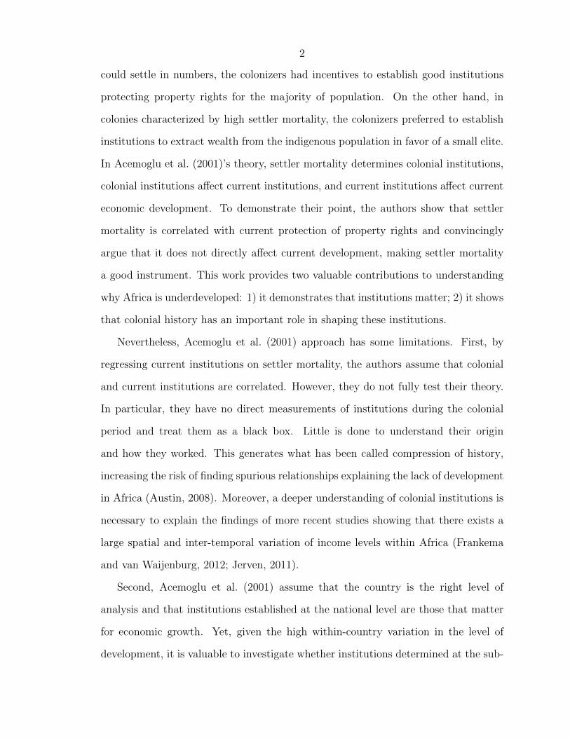
could settle in numbers, the colonizers had incentives to establish good institutions
protecting property rights for the majority of population. On the other hand, in
colonies characterized by high settler mortality, the colonizers preferred to establish
institutions to extract wealth from the indigenous population in favor of a small elite.
In Acemoglu et al. (2001)’s theory, settler mortality determines colonial institutions,
colonial institutions affect current institutions, and current institutions affect current
economic development. To demonstrate their point, the authors show that settler
mortality is correlated with current protection of property rights and convincingly
argue that it does not directly affect current development, making settler mortality
a good instrument. This work provides two valuable contributions to understanding
why Africa is underdeveloped: 1) it demonstrates that institutions matter; 2) it shows
that colonial history has an important role in shaping these institutions.
Nevertheless, Acemoglu et al. (2001) approach has some limitations. First, by
regressing current institutions on settler mortality, the authors assume that colonial
and current institutions are correlated. However, they do not fully test their theory.
In particular, they have no direct measurements of institutions during the colonial
period and treat them as a black box. Little is done to understand their origin
and how they worked. This generates what has been called compression of history,
increasing the risk of finding spurious relationships explaining the lack of development
in Africa (Austin, 2008). Moreover, a deeper understanding of colonial institutions is
necessary to explain the findings of more recent studies showing that there exists a
large spatial and inter-temporal variation of income levels within Africa (Frankema
and van Waijenburg, 2012; Jerven, 2011).
Second, Acemoglu et al. (2001) assume that the country is the right level of
analysis and that institutions established at the national level are those that matter
for economic growth. Yet, given the high within-country variation in the level of
development, it is valuable to investigate whether institutions determined at the sub-

3
national level are actually more important (Michalopoulos, 2012). For example, labor
market institutions might be affected mostly by local conditions, such as the kind of
agricultural production of each region.
Third, Acemoglu et al. (2001) acknowledge the fact that institutions evolved dur-
ing the colonial period and after independence, even if their extractive character
persisted. However, focusing on identifying an exogenous source of variation for insti-
tutions, they overlook how institutions change. Nevertheless we need to understand
these processes if we want to understand how to modify the extractive institutions
that hinder economic growth in Africa.
The paper by Acemoglu et al. (2001) generated a substantial amount of work about
colonialism and development in Africa. The subsequent literature moved away from
asking whether history matters to asking how history matters, identifying precisely
the channels of causality. This new approach relies on more sophisticated identifi-
cation techniques and micro-level data. Huillery (2009) uses district-level data and
matching estimators to show that colonial and current levels of schooling are corre-
lated. Gallego and Woodberry (2010) and Nunn (2010) employ data at the province
and ethnic group/village level to study the impact of colonial missionary activity on
schooling and religious conversion. Michalopoulos and Papaioannou (2011) exploit
ethnic group-level data to estimate the effect of arbitrary colonial borders on civil
war. Berger (2009) uses the historical border between Northern and Southern Nige-
ria and a regression discontinuity approach to study the modern impact of colonial
policies on public good provision. Cogneau and Moradi (2014) also employ a regres-
sion discontinuity technique to analyze the effect of colonial policies on education and
religion across the border between the French and British partitions of Togoland.
Nevertheless, despite valuable progresses in explaining how various colonial fea-
tures affect current development, the main limitations of Acemoglu et al. (2001) have
not been overcome yet. Much more limited efforts have been undertaken to quantify
4
colonial extraction, open the black box of extractive institutions, and understand their
role during the colonial period. To fully evaluate the implications of Acemoglu et al.
(2001)’s insight, we need to decompress history more than what has been attempted
so far in the literature. How can we define and quantify colonial extraction? Which
institutions were involved? What determined these institutions? Was the level of
extraction similar across colonies or economic activities? How did colonial extraction
persist over time and still affect current development?
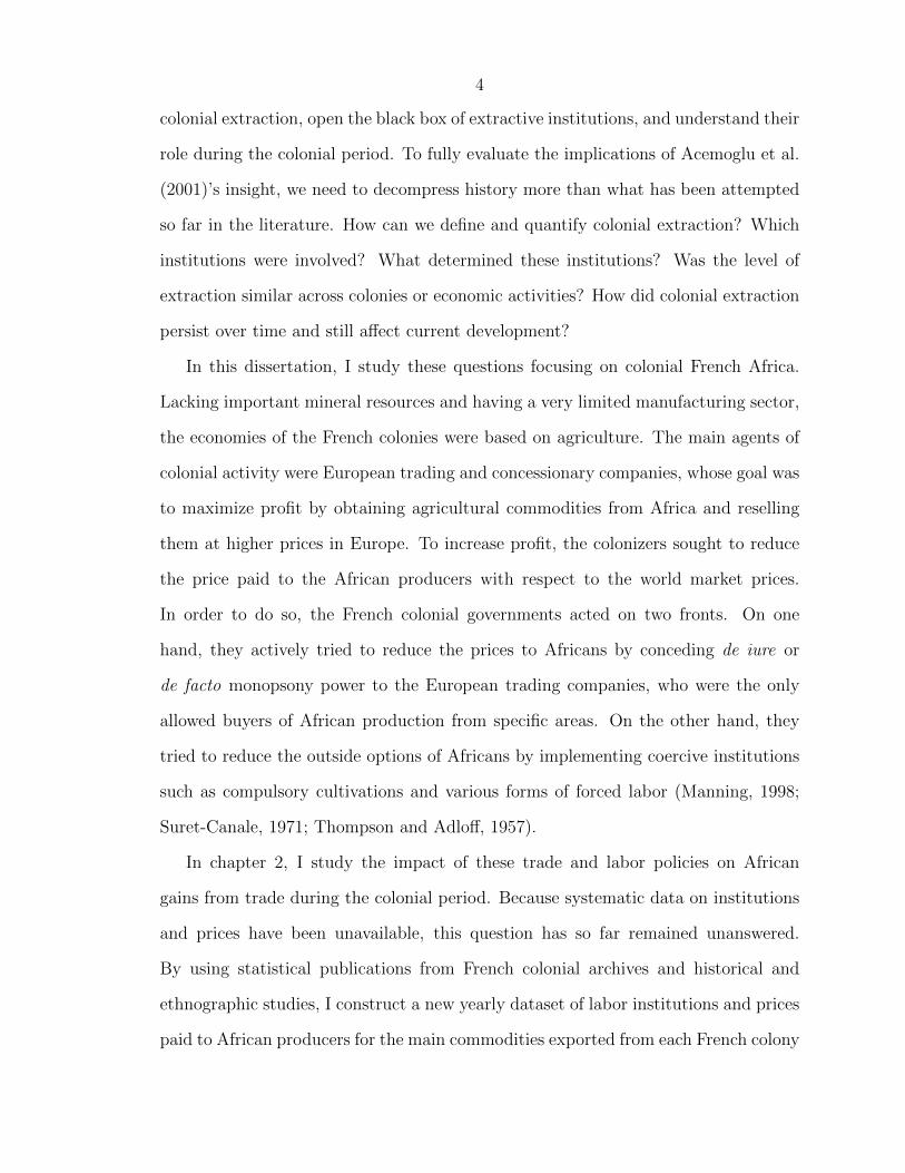
In this dissertation, I study these questions focusing on colonial French Africa.
Lacking important mineral resources and having a very limited manufacturing sector,
the economies of the French colonies were based on agriculture. The main agents of
colonial activity were European trading and concessionary companies, whose goal was
to maximize profit by obtaining agricultural commodities from Africa and reselling
them at higher prices in Europe. To increase profit, the colonizers sought to reduce
the price paid to the African producers with respect to the world market prices.
In order to do so, the French colonial governments acted on two fronts. On one
hand, they actively tried to reduce the prices to Africans by conceding de iure or
de facto monopsony power to the European trading companies, who were the only
allowed buyers of African production from specific areas. On the other hand, they
tried to reduce the outside options of Africans by implementing coercive institutions
such as compulsory cultivations and various forms of forced labor (Manning, 1998;
Suret-Canale, 1971; Thompson and Adloff, 1957).
In chapter 2, I study the impact of these trade and labor policies on African
gains from trade during the colonial period. Because systematic data on institutions
and prices have been unavailable, this question has so far remained unanswered.
By using statistical publications from French colonial archives and historical and
ethnographic studies, I construct a new yearly dataset of labor institutions and prices
paid to African producers for the main commodities exported from each French colony
5
between 1898 and 1959. By developing a theoretical model of trade under colonial
extraction and using panel data methods, I show that monopsonies and coercive labor
institutions reduced African gains from trade by at least 60%.
In chapter 3, I focus on the origin of coercive labor institutions by analyzing
the colonial governments’ incentives to choose between coerced and free labor. I
argue that the choice of institutions was affected more by the properties of exported
commodities, such as prices and economies of scale, than by the characteristics of
colonies, such indigenous population density and ease of settlement for the colonizers.
In chapter 4, I look at the effects of colonial institutions on current development.
Coercive labor institutions were abolished after independence, but de facto trad-
ing monopsonies persisted, and post-independence governments continued to practice
price policies that discriminated against agricultural producers. I show that the ex-
tent to which prices to agricultural producers were reduced in the colonial period
is strongly negatively correlated with current regional development, as proxied by
luminosity data from satellite images. I argue that colonial extraction reduced de-
velopment in rural areas and increased economic growth in cities. Despite this, the
overall impact on development is negative and the different effects in rural and urban
areas can actually be the reason why trade monopsonies and extractive institutions
persisted long after independence. Chapter 5 provides concluding remarks and sug-
gests directions for future research.

6
Chapter 2
Extractive Institutions and Gains
From Trade: Evidence from
Colonial Africa
2.1 Introduction
Many leading hypotheses about current African underdevelopment emphasize the role
of colonialism. If the early literature underlined how colonial rule relegated Africa
to exporter of primary commodities (Rodney, 1972), more recent works have instead
focused on the long-term consequences of colonial extractive institutions (e.g.,, Ace-
moglu et al., 2001, 2002; Englebert, 2000; Herbst, 2000; Nunn, 2007).1 Yet, to explain
how colonial institutions affect current development, we need to understand the ex-
tent of extraction during the colonial period. Many of the institutions established by
the colonizers were, in fact, maintained in the post-independence period. Moreover,
the extent to which they were extractive in the colonial period affects how extractive
1Extractive institutions can be defined as those arrangements “designed to extract incomes andwealth from one subset of society [masses, African populations] to benefit a different subset [elite,colonizers]” (Acemoglu and Robinson, 2012).

7
they are after independence (Acemoglu et al., 2001; Bates, 1981). However, since
colonial extraction is hard to quantify and its exact mechanisms are unclear, we still
do not know precisely how successful the colonizers were in extracting wealth from
Africans.
This chapter investigates this issue by exploiting the peculiar structure of labor
and trade policies employed by the French colonizers. The focus on trade in the
French colonies offers two main advantages for understanding the mechanisms of
extraction in the colonial period. First, because of the low population densities of
French Africa and the high cost of labor relative to land, the colonizers faced there
powerful incentives to use coercive labor institutions.2 Second, focusing on trade
allows us to use price data in order to evaluate colonial extraction. By using the
gap between prices to African agricultural producers and world market prices as a
measure of extraction, I analyze how colonial trade monopsonies and coercive labor
institutions affected African gains from trade during the colonial period.
Because of limited data on colonial institutions and prices in Africa, this question
has so far remained unanswered. On one hand, historians have collected information
about colonial institutions, but they have not attempted to systematically quantify
the level of extraction. On the other hand, economists have overlooked the temporal
variation in colonial extraction, increasing the risk of “compression of history” and
making it difficult to understand how extractive institutions persist over time (Austin,
2008).3
2When coercion is a feasible option, a higher land/labor ratio might not translate into higherwages, but in an increase of coercion of labor (Domar, 1969). Fenske (2013) tests this hypothesis inthe African context showing that lower population density is correlated to the extent of indigenousslavery.
3Previous works by economists exploited spatial variation in some colonial policy or institution,observed in one point in time. Huillery (2009) studies the impact of colonial investments in educationin French Africa. Gallego and Woodberry (2010) and Nunn (2010) analyze the effect of colonialmissionary activity on schooling and religious conversion. Michalopoulos and Papaioannou (2011)estimates the effect of arbitrary colonial borders on civil war. Berger (2009) studies the modernimpact of colonial policies on public good provision in Nigeria Cogneau and Moradi (2014) analyzesthe effect of colonial policies on education and religion across the border between the French andBritish partitions of Togoland.

8
My first contribution then is to provide a new yearly dataset of labor institutions
and prices paid to African producers for the main commodities exported from each
French colony between 1898 and 1959. I collected the data on labor institutions from
historical and ethnographic studies and the data on prices from a variety of colonial
publications, including, but not limited to, statistical reports of the Ministry of the
Colonies, customs statistics, and Bulletins Economiques of the different colonies.
My second contribution is to use these data to understand how colonial extractive
institutions affected African prices. The main difficulty in answering this question is
that, since extractive institutions were used in all colonies, we cannot observe colonial
trade in absence of extraction. However, since in a competitive market the prices to
African producers should be equal to the difference between world market prices and
transport costs, we can use this measure as a counterfactual.
Building on this insight, I proceed in three steps. First, I use my price dataset
to check whether colonial extraction (monopsony and coercive labor institutions)
implied a reduction in the prices to African producers. I show that the prices to
Africans were reduced by about 30% with respect to what they would have been
in absence of monopsonies and coercive labor institutions. Moreover, the level of
extraction varied substantially across the different colonies and economic activities
and decreased in the second half of the colonial period.
Second, I use newly collected data on labor institutions to disentangle the effect
of coercive labor institutions on prices to producers from the effect of monopsony.
I present evidence that the level of coercion of labor affected the extent of price
reduction. Prices to Africans were reduced by 25% with respect to competitive prices
if the colonizers used free peasant production, but they were reduced by almost 40%
for crops that were produced under compulsory cultivations.
To make sure that the relationship between prices and institutions is not spurious,
I need to consider potential omitted variables. One candidate is the price elasticity

9
of African supply. The colonizers might have in fact established coercive institutions
and offered lower prices in colonies/crops where Africans responded less to price
incentives. To account for this problem, I exploit the panel structure of the data and
the historical evidence on change in institutions. Since the transition from compulsory
to free production at the end of the colonial period was affected more by the political
climate before independence than by changes in elasticity of supply, I can reduce the
omitted variable bias by controlling for colony/commodity and year fixed effects.
Finally, I construct lower bounds for the losses that monopsony and coercive
labor institutions together implied for African welfare: on average, colonial extraction
reduced African gains from trade by over 60%. Moreover, by exploiting the insight of
a simple model of colonial trade under extractive institutions, I am able to disentangle
the effects of monopsony from those of coercive labor institutions. I show that, when
the latter were used, they accounted for at least 60% of the total losses.
The chapter is structured as follows. Section 3.2 provides some historical back-
ground about French colonies in Sub-Saharan Africa, monopsonistic trading compa-
nies, and labor institutions. Section 2.3 proposes a theoretical model of colonial trade
under extractive institutions. The following three sections test the implications of the
model: Section 2.4 explores the effect of colonial extraction on prices to Africans, Sec-
tion 2.5 focuses on the impact of coercive labor institutions, and Section 2.6 provides
lower bounds for the reduction in the gains from trade with respect to competition.
Section 2.7 offers concluding remarks and delineates directions of future research.
2.2 Historical Background
Most of the military conquest of French Africa occurred between 1880 and 1900.
Towards the end of 19th century there still existed some small pockets of resistance
(Mauritania did not fall under full French control until 1936), but the conditions

10
were ready for the development of the colonial system (Coquery-Vidrovitch, 1969;
Suret-Canale, 1971).
The French government organized the colonies in two federations: French West
Africa (1895)—including Mauritania, Senegal, French Sudan (now Mali), Niger, Up-
per Volta (now Burkina Faso), Guinea, Cote d’Ivoire, and Dahomey (now Benin)—
and French Equatorial Africa (1908)—including Gabon, Congo, Ubangi-Shari (now
Central African Republic), and Chad. After WW1, part of Togo and almost all of
Cameroon were added to the French colonies in continental Sub-Saharan Africa (see
Figure 2.1).
Figure 2.1French West and Equatorial Africa
Togo and Cameron were not part of AOF and AEF, but they were traditionally included in West
and Equatorial French Africa, respectively.
The extension of French possessions was reflected in the heterogeneity of their
natural environment, including, from the coast towards the interior, tropical forests,
savannas, and arid-desertic regions. The coastal forestry regions were suitable to

11
produce bananas, coffee, cocoa, and rubber, while the drier interior areas were suitable
for peanuts and cotton. In general, Western colonies were more prosperous than
Equatorial colonies and, with the exception of the peanut-producing areas of Senegal,
coastal regions were usually wealthier with respect to interior regions because of the
higher value of their crops and lower transportation costs (Hopkins, 1973).
Figure 2.2 shows the evolution of the total value of exports (in constant 1900
francs, evaluated with prices in France) from French Africa between 1900 and 1960.4
Exports grew during the entire colonial period, slowed down throughout the Great
Depression, and increased dramatically after 1945. On average, peanuts accounted for
the highest share of exports (about 30% of the total value), followed by rubber (about
18%), oil palm produces (15%), coffee, cocoa, and timber (each of them accounting
for about 10%). Cotton and bananas accounted for the remaining exports. Cote
d’Ivoire, Senegal, and Cameroon were the richest colonies, generating 28%, 21%, and
16% of the total value of exports, respectively.
Given the variety of environments and commodities, the colonizers structured
economic activity and trade in the colonies in different ways. In West Africa, exports
were initially based only on African peasant production. European trading companies
limited themselves to buying crops and reselling them at higher prices in Europe.
After WWI, Europeans began to enter the productive sector, establishing plantations
(e.g.,, cocoa and coffee in Cote d’Ivoire, bananas in Guinea) and exploiting forestry
concessions. Mining was a minor activity. In Equatorial Africa economic activity was
initially organized on the basis of concessionary companies with monopoly over given
territories. African laborers were forced to collect crops, especially rubber, for the
concessionaires who employed harsh coercive methods. The abuses of the concession
system led to its termination in the 1920s, when trading companies on the model of
West Africa were established (Suret-Canale, 1971).
4See Section 2.4.1 for details on the data.

12
Figure 2.2Total Value of Exports from French West and Equatorial Africa
The total value of exports is in millions of 1900 French francs, evaluated using prices in France net of
trading costs. It includes all the main commodities (bananas, cocoa, coffee, cotton, peanuts, oil palm
produces, rubber, and timber) and all colonies. Values are computed as 10-years averages to reduce
the impact of outliers and to have at least one observation for each colony/commodity/decade.
Missing data are interpolated.
13
The French administration fixed the import prices in France by ministerial decree,
following world market prices, and the prices to African producers, usually as a per-
centage of the world market price. For example, cotton price paid to Ubangi-Shari
farmers was 15% of the average FOB price of cotton in New York (DeDampierre,
1960).
Whether the economic activity was organized through European companies or
African peasant agriculture, the French colonizers had incentives to reduce the cost of
production in order to increase profit. Thus, the colonial government tried to establish
de iure or de facto monopsonies for the trading and concessionary companies in order
to reduce prices and wages to Africans (Coquery-Vidrovitch, 1972; Manning, 1998;
Suret-Canale, 1971; Thompson and Adloff, 1957).
At the beginning of the 20th century, trade in the Senegal/Mali region was con-
trolled by a group of eight Bordeaux trading firms, while Guinea and Congo were in
the hands of business houses from Marseilles or Paris. Smaller traders were allowed
a share of exports as long as they respected the prices fixed by the main trading
firms. After WWI, the de facto monopsony of these companies grew stronger: eco-
nomic crises eliminated competition from smaller companies, German business inter-
ests were canceled by the war, and protectionist measures were taken against British
trade. Protectionist policies were not applied everywhere and did not completely
eliminate non-French trade (especially in Guinea and Dahomey). Nevertheless, the
number of the remaining trading firms became sufficiently small to allow agreement
and ban entry into the African market (Suret-Canale, 1971). As a result, at the
beginning of WWII, fewer than a dozen companies monopolized almost all of trade
from French West Africa and two French companies (Societe Commerciale de l’Ouest
Africain, Compagnie francaise de l’Afrique Occidentale) and a British one (Unilever)
controlled between 50% and 90% of exports (Suret-Canale, 1971, p. 167).
In addition to establishing monopsony power for the trading companies, the col-

14
onizers attempted to reduce price and wages to Africans by interfering with labor
markets and implementing coercive institutions.5 Since capital was relatively expen-
sive, production relied on labor-intensive methods. French Africa’s low population
densities and abundant cultivable land in the indigenous sector implied that African
incentives to enter the wage labor force or to produce cash crops were insufficient.
For these reasons, the colonizers put in place specific institutions such as compul-
sory African cultivations and various forms of forced labor in European plantations.
These institutions, by reducing the outside options of Africans, had to goal to further
increase the ability of the colonial governments to lower prices to producers.
Three main kind of institutions were used (free peasant production, compulsory
peasant production, and concession/forced labor production) and the type of coercive
arrangements available to the colonizers depended on whether agricultural production
was African-based or European-based. When the colonizers limited themselves to
trade and production was left to African peasants, the colonial governments could
introduce compulsory peasant production. In this case, they set quotas that Africans
had to produce and sell for a fix price to the colonizers. The most notable example
of this institution were the cotton quotas established by Felix Eboue in Ubangi-Shari
in 1924 (DeDampierre, 1960). Under this arrangement, every village had to produce
amounts of cotton in proportion to its population and sell it to trading companies
with monopsony power over given territories. The costs for the recruitment of cotton
producers were borne by the colonial government, and payments were often in the
form of tax vouchers. Cotton quotas were abolished in 1956, just four years before
independence.
Alternatively, when the colonizers entered the productive sector, establishing con-
cessions and plantations, forced labor could be implemented. It took the direct form
of labor taxes and the indirect form of contract labor. With labor taxes, all males
5We can interpret these institutions as subsidies given by the colonial government to the Europeantrading and concessionary companies.

15
between 18 and 60 had to contribute a certain number of days of unpaid labor (usu-
ally from 8 to 12 per year) to whatever enterprise the administration assigned them.
Labor taxes were used mostly for porterage and public works, but not infrequently
for private enterprises, especially in the early days of the colonial period. They were
finally abolished for both the private and public sector in 1946 (Fall, 1993).6 Con-
tract labor was a system of formal labor recruiting used mainly for private enterprises.
While not forced labor, it was far from a free market system. The most important
figure in this system was the labor recruiter who rounded up manpower in villages.
Local chiefs received payments for every man supplied and were therefore encouraged
to cooperate with the recruiter. The compulsory nature of this system decreased in
the late 1930s, when freer forms of recruitment started to appear.
However, coercive labor institutions were not implemented everywhere. When
neither compulsory cultivations nor forced labor were used, the prices or wages were
still fixed by the colonizers, but the African peasants could decide whether to work for
the colonizers in the case of European-based production or how much crop to produce
in the case of African-based production. Free peasant production was actually used
in the majority of cases, accounting for almost 60% of the total value of exports;
concession and compulsory production followed with about 30% and 10% of the export
value, respectively.
Given such a variety of labor arrangements, one might ask which factors affected
the kind of institutions that were implemented. In chapter 3, I will show that the
choice was affected more by factors related to the characteristics of crops, such as
economies of scale and world prices, than to the characteristics of colonies, such
as settler mortality or population density. Free peasant production was used for
low-value crops with limited economies of scale (peanuts, palm kernels, and cocoa).
Compulsory peasant production was implemented for crop with limited economies
6Other institutions such as labor drafts, convict labor, and military labor worked in a similarmanner.

16
of scale , but high value (cotton, wild rubber). Concession production with various
forms of coercion for African workers was used for commodities whose production
needed large capital investments and was characterized by large economies of scale
(bananas, coffee, timber, plantation rubber).
Nevertheless, some variation in institutions existed across regions and time within
the same crop. Free peasant production was much more diffuse in West African
colonies, while concession production and especially compulsory production were em-
ployed more frequently in Equatorial Africa. Over time, and in particular after WWII,
the political pressure to abolish coercive institutions increased. As a result, we ob-
serve a transition towards free peasant production in most colonies and crops. At the
onset of independence, free peasant production accounted for almost 70% of the total
value of exports, with the remainder produced under concessions.
2.3 A Model of Colonial Extraction
Although both economists and historians agree on the importance of colonial insti-
tutions, the extent of extraction has been difficult to assess. How much did colonial
extractive institutions reduce African prices and gains from trade?
In order to answer this question, we need to identify the proper counterfactual. To
do so, I outline a simple model of colonial trade under monopsony and coercive labor
institutions. For the purpose of the model, institutions are treated as exogenous, and
I will address the issue of their origin in the empirical part of the chapter.
There are two groups of actors: African Peasants and Trading Companies. The
African Peasants produce one crop and sell it to the Trading Companies. The Trading
Companies set the price to producers and resell the crop at the world market price in
Europe.7 Given the price to producers pA, the African Peasants produce the quantity
Q in order to maximize ΠA = pAQ − C(Q), where C(Q) is a convex cost function.
7The traded quantity from Africa is too small to affect world prices. See Table 3.1.

17
The FOC implies that the quantity is such that the marginal cost is equal to the price
and the African supply function is Q(pA) = MC−1(pA), where MC is the marginal
cost function. Given this supply function, the Trading Companies choose the price
pA to maximize ΠC = (p − t − pA)Q(pA), where p is the (exogenous) world market
price and t are transportation costs. The price paid to Africans varies according to
the kind of institutions governing trade and production: perfect competition among
trading companies, simple monopsony, monopsony and coercive labor institutions.
Let us consider each of the three cases.
1. Perfect Competition
Suppose that there are (infinitely) many trading companies competing for African
production. If one company sets a price pA < p − t, then a second company
might set a higher price, buy the entire production, and still make a positive
profit. The equilibrium price to Africans is just the difference between price in
Europe and transport costs,
pA = p− t (2.1)
In this case, the profit of the Trading Companies is zero.
2. Simple Monopsony
Suppose that one Trading Company has the right to buy all African production.
In this case, the FOC for the Trading Company’s maximization problem implies
pA = p− t− Q(pA)
Q′(pA)(2.2)
Since both Q(pA) and Q′(pA) are positive, the price to Africans is lower under
monopsony than under competition. In this case, the Trading Company makes
a positive profit.
3. Monopsony and Coercive Labor Institutions

18
Suppose that, in addition to monopsony, the Trading Company has access to
coercive labor institutions (various forms of forced labor and compulsory cul-
tivations) in order to force African Peasants to produce more than they would
produce at any given price. We can model African’s supply function under co-
ercive institutions as Qc(pA) = Q(pA + c), where c is the level of coercion. In
this case, the FOC implies
pA = p− t− Q(pA + c)
Q′(pA + c)(2.3)
Since Q(.) is increasing and concave, Q(pA+c)Q′(pA+c)
> Q(pA)Q′(pA)
. Thus, the price under
monopsony and coercive labor institutions is lower than the price under simple
monopsony. As a consequence, the profit of the Trading Company is higher in
this last case.
Let us now consider the implications of these institutional arrangements for African
gains from trade.
• Simple Monopsony
Since the price under simple monopsony is lower than the price under com-
petition, the traded quantity will also be lower. African gains from trade are
thus lower under simple monopsony than under competition. Without coercive
labor institutions the marginal cost of each unit is always lower than the price,
so Africans still get some gains from trading, but less than if they were facing
competition among trading firms.
• Monopsony and Coercive Labor Institutions
With coercive labor institutions, the price is lower than under simple monop-
sony. Given the presence of coercion, the traded quantity is higher, but Africans
will produce the additional quantity at a cost higher to the price. For this rea-

19
son, African gains from trade are lower under monopsony and coercive labor
institutions than under simple monopsony. Moreover, notice that, because the
Africans receive a price lower than the marginal cost, they might be worse off
with respect to not trading at all.
The model yields three predictions about the features of colonial extraction in French
Africa:
1. Prices to Africans were lower than they would have been with competition.
2. They were further reduced with respect to monopsony prices by the presence of
coercive labor institutions.
3. Extractive institutions reduced African gains from trade.
In the rest of the chapter, I will empirically test these results.
2.4 Result 1: Prices to Africans and Competitive
Prices
In this section I explore the first result of the model, checking whether the prices to
Africans in the French colonies were lower than competitive prices.
2.4.1 Data
To test this hypothesis, I use newly-collected data on prices in Africa, prices in France,
and transport costs. I focus on nine main commodities exported by French Africa:
peanuts, palm kernels and oil, cotton, cocoa, coffee, rubber, timber, and bananas.
The commodities included in the dataset account for 80% of the value of all exports
from West and Equatorial Africa during the whole colonial period.
Prices in Africa and Quantities Exported

20
Colonial customs statistics reported the total quantity and value for each exported
commodity from each colony every year. These statistics were registered at the local
customs offices and then aggregated at the colony level. The reported values were
usually official market prices in Africa (valeurs mercuriales), established by decree
by the General Governor of the colonies on the basis of reports of local commissions
of evaluation. After World War II, the reported evaluations were often values of the
commodities at the loading port, including transportation costs to the port and exit
taxes.8
Table 2.1Components of Prices: Cocoa, 1958–59
Togo Congo Cote d’Ivoireprice to producers 100 82 90transport to port 4 12 5taxes, insurances, stockage 32 30 31price at African port 136 124 126
Source: elaboration from Documents et statistiques—Ministre de la
France d’Outre-mer, Service de statistique, 1958–59. Prices are in
current francs per kg.
Using these customs statistics, I collected data on prices in Africa and quantities
exported from each colony for nine main commodities between 1898 and 1959. I
exploited numerous yearly issues of different colonial publications, including, but not
limited to, statistical reports of the Ministry of Colonies, Bulletins Economiques of
the various colonies, and Annuaire Statiques of West and Equatorial Africa.9
Given the variety of the sources and the length of the period considered, the
names of the territorial units for which the custom statistics are reported change over
time and sometimes data are reported only for larger territorial units. To solve these
issues, I first tracked the variation in the names of colonies. Then, I assigned each
8These values are a good proxy for the actual prices to producers: detailed data on prices tofarmers, inland transport cost, and tariffs from the late 1950s show that, after controlling for trans-portations costs, differences in prices at African ports are almost exclusively due to differences inprices to producers. See Table 2.1.
9See the appendix for more details on the sources.

21
commodity from a larger territorial unit to the smallest territory (colony or group of
colonies) that I could identify by excluding those colonies which do not produce that
specific commodity.10 I deflated all prices in 1900 French francs.11
Prices in France
I collected prices in France from various issues of the Statistiques Mensuelles du
Commerce Exterieur de la France, a monthly publication by the Direction Generale
des Douanes reporting the total values and quantities of the commodities imported
from the French colonies in every year. As a control, I also used different issues of the
Annuaire Statistiques de France reporting similar information. I deflated all prices in
1900 French francs.
Not all exports from French Africa went to France. Nevertheless, given the impor-
tance of the French market, using export prices in France is a good approximation.
By 1949, France was the destination of about 80% of the total exports originating
from its African colonies (Duignan and Gahan, 1975). Moreover, French prices are
highly correlated with world market prices, as shown in appendix 2.8.1.
Transport costs
Since extensive data on transportation costs between Africa and France are not
available, I constructed estimates of shipping costs for each colony-commodity-year
in my dataset according to the following procedure. First, I computed the distance
to Marseilles from the closest African port for each colony.12 Then, I used data on
average freight rates from the West African coast to France for the main exports in
1938 to compute the average shipping cost per km for each commodity in 1938.13
Finally, I multiplied this measure by the distance to Marseilles for each colony (both
10For example, all cocoa exports 1898–1907 recorded as from French Congo (including Gabon andCongo) are assigned to Gabon because there was no registered cocoa production in Congo before1927. Territorial units involved are AEF, French Congo, AOF, and Senegal-Haut Senegal-Niger.
11Inflation data come from France-Inflation.com (2013).12The main ports are identified from the map reported at page 149 of Duignan and Gahan (1975).
The distance to Marseille is computed by using http://ports.com/sea-route.13Documents et statistiques—Ministere de la France d’Outremer, Service de statistique, 1949–52.
22
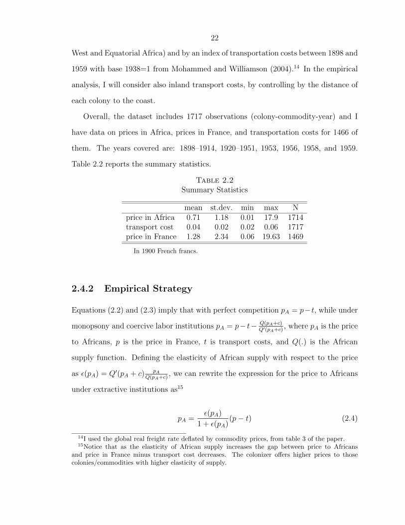
West and Equatorial Africa) and by an index of transportation costs between 1898 and
1959 with base 1938=1 from Mohammed and Williamson (2004).14 In the empirical
analysis, I will consider also inland transport costs, by controlling by the distance of
each colony to the coast.
Overall, the dataset includes 1717 observations (colony-commodity-year) and I
have data on prices in Africa, prices in France, and transportation costs for 1466 of
them. The years covered are: 1898–1914, 1920–1951, 1953, 1956, 1958, and 1959.
Table 2.2 reports the summary statistics.
Table 2.2Summary Statistics
mean st.dev. min max Nprice in Africa 0.71 1.18 0.01 17.9 1714transport cost 0.04 0.02 0.02 0.06 1717price in France 1.28 2.34 0.06 19.63 1469
In 1900 French francs.
2.4.2 Empirical Strategy
Equations (2.2) and (2.3) imply that with perfect competition pA = p−t, while under
monopsony and coercive labor institutions pA = p− t− Q(pA+c)Q′(pA+c)
, where pA is the price
to Africans, p is the price in France, t is transport costs, and Q(.) is the African
supply function. Defining the elasticity of African supply with respect to the price
as ε(pA) = Q′(pA + c) pAQ(pA+c)
, we can rewrite the expression for the price to Africans
under extractive institutions as15
pA =ε(pA)
1 + ε(pA)(p− t) (2.4)
14I used the global real freight rate deflated by commodity prices, from table 3 of the paper.15Notice that as the elasticity of African supply increases the gap between price to Africans
and price in France minus transport cost decreases. The colonizer offers higher prices to thosecolonies/commodities with higher elasticity of supply.

23
We can thus test whether the prices to Africans were lower than they would have
been with competition by running the following regression
pA,cit = β(pct − tcit) + ucit (2.5)
where c refers to the commodity, i to the colony, t to time, and ucit is the error term.
Under the null hypothesis and no colonial extraction, β = 1.16
However, the estimation of β is likely to be inconsistent because transport costs
t might not include all of the costs that the trading companies had to face to export
commodities from Africa to France (e.g.,, loading and storage costs, taxes and tariffs,
insurances). Suppose that the true regression is pA,cit = β(pct − tcit − ccit) + εcit,
where ccit represents other omitted costs. Assume Cov(p, ε) = 0, Cov(t, ε) = 0,
and Cov(c, ε) = 0. Standard results imply that, estimating β by OLS from (2.5),
plimβOLS = β(1 − Cov(p,c)−Cov(t,c)V ar(p−t) ). If Cov(p, c) − Cov(t, c) > 0, then the estimated
coefficient is biased against the null hypothesis of no extraction.
Fixed transport costs (loading and unloading, warehousing, insurance, docking
fees, etc.), inland transport costs from the interior to the port, and taxes and tariffs
in Africa and in France are likely to be omitted costs. Even if it is reasonable to think
that the correlation of fixed and inland transport cost with t is positive (implying a
potential bias in favor of the null), the correlation between prices in France and
omitted costs could also be positive, leaving the direction of the bias ambiguous.
Suppose, for example, that the price of a commodity in France is equal to the price
of that commodity in a big supplier country plus fixed transport costs and shipping
costs from there to France. If fixed transport costs in this country are the same
or correlated with fixed transport costs in Africa, then Cov(p, c) > 0. Moreover, if
16In equation (2.5) the coefficient β is equal to ε(pA)1+ε(pA) and thus it might depend on pA. This
is not an issue if we assume a supply function with constant elasticity of supply, such as the oneoriginated from a Cobb-Douglas production function with decreasing return of scale.

24
transport costs depend on some characteristics of commodities (perishability, stowage
factors, etc.), inland and fixed transport costs might be positively correlated and
consequently also inland transport costs and prices in France would be positively
correlated. Finally, the colonizers might tax more heavily commodities with higher
values, implying again Cov(p, c) > 0.
To reduce the impact of omitted variables, I pursue two strategies. First, I control
for observables including proxies for fixed and inland transportation costs. Second, I
control for unobservables using fixed effects.
Controlling for observables
To control for fixed transport costs, I use the value of fixed transport costs esti-
mated by Maurer and Yu (2008, p.693) for the Panama Canal: 2.12 $ per ton in 1925
(3.12$ minus 1$ of Panama Canal tolls). Considering an exchange rate of 21 francs
per $ in 1925 and deflating in 1900 francs, this corresponds to 9.64 1900 francs per
ton in 1925. I multiply this value by the index in Mohammed and Williamson (2004)
with base 1925 to get fixed transport costs for every year. Notice that including
this fixed cost measure might mean double-counting fixed costs since they could be
already included in my original shipping cost data.
To control for inland transport costs, for each colony I include in the regression
the average distance from the interior to the coast.17 Moreover, since the ratio vol-
ume/weight is an important determinant of both fixed (loading and warehousing) and
inland transport costs, I also control for each commodity’s stowage factor.18
Controlling for unobservables
I model unobservable costs as ccit = kci + θt. The first component k captures
the differences in costs due to each commodity-colony; the second component θ cap-
tures the variation over time, common to all commodities-colonies. This is a mild
assumption: I allow unobservable costs to vary across commodity-colony and time,
17GIS World Geography Datasets, Portland State University.18Source is http://www.cargohandbook.com.

25
just assuming a common trend over time in all colonies and commodities. In the
empirical specification, I implement this idea by using commodity/colony and time
fixed effects. In this way, the relationship between price in France minus transport
costs and price in Africa is identified exclusively from the variation within each com-
modity/colony over time, after taking into account common time shocks affecting all
commodities and all colonies.
I estimate the following regression
pA,cit = β(pct − tcit − fcit) + (Xcitδ) + kci + θt + εcit (2.6)
where f is the proxy for fixed transport costs, X is a vector of control variables
including distance from the coast and commodity’s stowage factor (excluded when
I include fixed effects), and k and θ are commodity/colony and time fixed effects,
respectively. If there is no extraction, β = 1 (null hypothesis). If there is extraction,
β < 1.
A last concern regards measurement errors in my estimation of shipping costs
described in Section 2.4.1. Classic measurement error in t, in fact, would bias the
coefficient β towards zero, in favor of my hypothesis. To check whether this affects
the results, I run an alternative specification in which shipping costs are estimated
directly from the data. To do so, I exclude t from the regression and I control for
the interaction of distance to France with decade/commodity dummies.19 I run the
following regression
pA,cit = α + β1(pct − fcit) +Wct ∗Diη + εcit (2.7)
where Wct is a matrix of decade by commodity fixed effects and Di is the distance
19If I interacted the distance with year/commodity dummies, I would have too many fixed effectsand it would be difficult to estimate precisely the parameters.

26
from France. Each element of the vector of coefficients η measures the shipping cost
per km for each commodity and decade.
2.4.3 Results
Before presenting the results of the regressions, let me show some preliminary evidence
by comparing price gaps between Africa and France to those between US and UK.
The idea is that if the Africa-France price gap was larger than the price gap between
the United States and Britain, this would suggest that the difference between prices
in Africa and in France was not due exclusively to trading costs.
To check this, I collected yearly data on wholesale cotton prices in New York and
Liverpool between 1898 and 1938.20 Table 2.3 reports the percentage price gap in the
two markets for 5-year periods. The results show that, on average, the percentage
price difference between France and the colonies was about 12 times higher than the
difference between UK and US.
Table 2.3Cotton Price Gap between UK and US vs. France and French
Africa
price UK- price US price France- price Africaprice US price Africa
1898–1902 0.12 ..1903–1907 0.10 6.271908–1912 0.09 1.621913–1917 0.19 2.251918–1922 0.12 0.771923–1927 0.06 1.401928–1932 0.17 0.321933–1938 0.15 0.54
Sources: see text.
Given its magnitude, this results is unlikely to be driven by differences in shipping
costs. In the period under consideration, overall shipping costs from Africa to France
20My sources are the Historical Statistics of the United States (1975) and the Mitchell’s Abstractof British Historical Statistics (1988).
27
were about 4 times higher than between US and UK.21 Since prices in Africa were
about half of prices in the US, if the price gap was due only to shipping costs, then
the Africa-France relative price gap should have been only twice the US-UK price
gap. Similarly, the result is not driven by inland transport costs which accounted for
a small portion of the total costs.22
Table 2.4 presents the results of regression (2.6). Column (1) reports the simple
regression of price in Africa on the difference between price in France and shipping
and fixed transport costs: the coefficient is significantly less than 1 and we can reject
the null hypothesis that the price to Africans was just equal to the price in France
minus trading costs.
21Costs per km are on average 3.4 times higher between Africa and France than between US andUK (Maurer and Yu, 2008, table 4). Conversion rates are from www.measuringworth.com.) Thedistance between cotton producing French Africa to France (about 7300 km) is 15% higher that thedistance from New York to Liverpool (about 6400 km).
22According to the estimates of column (2) of table (2.4), one standard deviation increase indistance from the coast makes the price to Africans decrease by only .03 standard deviations.

28
Table2.4
Pri
cein
Afr
ica
vs.
Pri
cein
Fra
nce
Net
ofT
radin
gC
osts
Dep
enden
tva
riab
leis
pri
cein
Afr
ica
(1)
(2)
(3)
(4)
pri
cein
Fra
nce
net
ofsh
ippin
gan
dfixed
cost
s0.
47**
*0.
46**
*0.
41**
*(0
.03)
(0.0
3)(0
.05)
pri
cein
Fra
nce
net
offixed
cost
s0.
29**
*(.
09)
stow
age
fact
or(m
3/to
n)
-0.1
0**
(0.0
4)dis
tance
from
coas
t*(y
ear<
1945
),00
0skm
-0.1
2*(0
.07)
year
FE
Yes
com
modit
y*
colo
ny
FE
Yes
dis
tance
*dec
ade*
com
modit
yY
esR
20.
770.
770.
830.
82N
1466
1466
1466
1466
Res
ult
sfr
omre
gres
sion
(2.6
).S
tan
dard
erro
rscl
ust
ered
at
the
colo
ny/co
mm
od
ity
leve
lare
rep
ort
ed
inp
aren
thes
is.
***
p<
10%
,**p<
5%
,*p<
10%
.

29
In column (2) I control for other omitted costs, by including stowage factors and
distance to the coast. Since prices in Africa are measured at the export port after
WWII, I only include the distance from the coast for the years before 1945. The
main result is unaffected. In column (3) I control for unobservable costs, by using
commodity/colony and year fixed effects. Since fixed effects absorb all the variation
in stowage factor and distance from the coast, I exclude these control variables from
this specification. The coefficient of interest is still significantly less than 1.
The results of table 2.4 are unlikely to be driven by omitted costs. First, including
fixed effects, the R2 does not increase much: omitted costs are not a big determinant
of the price in Africa. Second, consider that the price in Africa is on average 55%
of the price in France and observable trading costs are about 5%: if the difference
was just due to omitted costs, unobservable costs should be 8 times the observable
costs. Finally, consider also that the ratio between origin FOB prices and destination
CIF prices from the FAO Agricultural Trade Database since 1960 is 89%, much larger
than the 55% ratio observed in the French colonies.
In column (4) I run regression (2.7), where shipping costs are estimated directly
from the data. The coefficient of interest is again significantly less than 1. Moreover,
since it is smaller than in column (1), this suggests that the bias of the estimates in
column (1) is against my hypothesis. My estimates of transport costs are not affected
by classic measurement errors and they are likely to overestimate real transport costs.
The evidence shows that prices in Africa were lower than competitive prices. Was
the extent of price reduction common to all colonies and crops? To answer this
question, I constructed an index measuring how much the price to Africans under
monopsony and coercive labor institutions was reduced as a proportion of how much
it should have been under competition and free labor
E =pcompetitionA − pextractionA
pcompetitionA
=p− T − pAp− T
= 1− pAp− T
(2.8)

30
where T includes shipping costs, fixed costs, and inland transport costs.23
On average, prices to Africans were reduced by about 30% because of colonial
extraction. Table 2.5 reports the average index for the different commodities in
West and Equatorial colonies. The average reduction varied across commodities: the
price was reduced by more than 40% for rubber and timber, by 35-40% for cotton
and bananas, by 25-30% for cocoa, coffee, and peanuts; and by 20-25% for palm
kernel and palm oil. Overall, the effects of colonial extraction were more severe in
Equatorial Africa (reduction of 37%) than in West Africa (29%) and the difference
was particularly large for palm kernel, coffee, palm oil, and timber.
Table 2.5Reduction of African Prices, as Percentage of
Competitive Prices
(1) (2)West Africa Equatorial Africa
average commodity 0.29 0.37bananas 0.36 0.37cocoa 0.27 0.32coffee 0.21 0.30cotton 0.37 0.35palm kernel 0.15 0.30palm oil 0.20 0.28peanut 0.21 0.41rubber 0.46 0.46timber 0.38 0.46
The table shows the average of price reduction indexes defined
in equation (4.1), by commodity and region.
Figure 2.3 shows the proportional reduction of prices to Africans due to colonial
extraction over time, for an average commodity/colony. Excluding WWII, over time
prices to Africans approach competitive prices. Looking at the figure, we can observe
that there was a change around the middle of the colonial period: before 1930, the
23Since the trading costs T tend to be overestimated, the index is sometimes greater than 1 (ifT > p) or less than 0 (if T > p− pA). In my analysis, I will therefore exclude all observations whoseindex is not between 0 and 1.
31
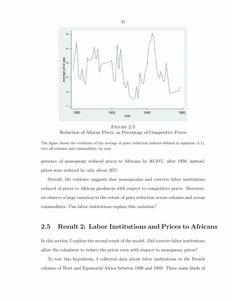
Figure 2.3Reduction of African Prices, as Percentage of Competitive Prices
The figure shows the evolution of the average of price reduction indexes defined in equation (4.1),
over all colonies and commodities, by year.
presence of monopsony reduced prices to Africans by 30-50%; after 1930, instead,
prices were reduced by only about 20%.
Overall, the evidence suggests that monopsonies and coercive labor institutions
reduced of prices to African producers with respect to competitive prices. Moreover,
we observe a large variation in the extent of price reduction across colonies and across
commodities. Can labor institutions explain this variation?
2.5 Result 2: Labor Institutions and Prices to Africans
In this section, I explore the second result of the model. Did coercive labor institutions
allow the colonizers to reduce the prices even with respect to monopsony prices?
To test this hypothesis, I collected data about labor institutions in the French
colonies of West and Equatorial Africa between 1898 and 1959. Three main kinds of

32
labor institutions were used.
• Free peasant production: the colonizer fixed the prices, but the African peasants
were free to produce how much they wanted at the given price.
• Compulsory peasant production: the colonizer fixed both prices and compulsory
quotas of production that had to be met by the African peasants.
• Concession production: production was run by the colonizer who used various
levels of compulsion to get African labor force.
Historians and ethnographers have gathered information about the institutional ar-
rangements used in the production of different crops in the various colonies, in general
works about French colonization or country-specific studies. For example, Coquery-
Vidrovitch (1972) wrote about rubber quotas in Congo in 1910s, while Suret-Canale
(1971) analyzed free peasant production of peanuts in Senegal. By systematically
extracting information from this literature, I was able to associate one of the three
labor institutions - free production, compulsory production, or concession production
- with each colony, commodity, and year.24
As shown in section 3.2, most of the variation in institutions was across crops:
peanuts and palms were mostly produced by free peasant production; cotton and
rubber by compulsory peasant production; timber, coffee, and bananas were usually
produced in European concessions. Equatorial colonies relied heavily on concessions
and compulsory production, while in West Africa free peasant production was more
diffused. Over time, we observe a decrease in the level of compulsion and an increase
in the extent of free peasant production.
I start the analysis of the impact of extractive institutions on prices to Africans
by treating institutions as exogenous. I will address the endogeneity issue later in
this section. To check whether coercive labor institutions can explain price gaps, I
24See the appendix for the sources.

33
regress the price to Africans on institution dummy variables
pAcit = α+ β1(COMPULSORY ) + β2(CONCESSION) +Zcitγ + η(p− T )cit + εcit
(2.9)
where free peasant production is the omitted category, Zcit is a vector of control
variables (including elasticity of African supply and colony/commodity, and year
fixed effects) and (p− T )cit is the competitive price.
We expect β1 < 0: the prices should be lower under compulsory peasant produc-
tion than under free peasant production. Instead, we expect β2 > 0: the prices should
be higher when European companies run production than when production is run by
African peasants. In the case of concessions, in fact, since the profit from colonial
trade has to be shared between the trading and the concessionary company, the prices
at African ports should be higher. Notice that this does not necessarily mean that
the level of extraction from African workers is lower under concession production, but
just that the export prices of commodities should be higher with respect to peasant
production.25
A potential concern with this approach is that the price elasticity of African sup-
ply might have affected both prices and institutions. The colonizer might have, in
fact, given lower prices to those colonies/commodities that responded less to price in-
centives (low elasticity of supply). At the same time, the colonizer might have needed
to establish coercive institutions to stimulate production where Africans responded
less to price incentive. If this was the case, the coefficient β1 would be biased in favor
of my hypothesis and the negative relationship between compulsory production and
prices would be spurious.
To solve this problem, I use two strategies. As a first strategy, I exploit the model
25We can write a similar model to that of section 2.3 in which: 1) Africans choose the number ofworkers L to maximize wL − c(L), where w is the wage and c(L) convex is the outside option; 2)the concessionary company chooses w to maximize pAf(L(w)) − wL, where f(.) is the productionfunction; 3) the trading companies chooses the price pA to pay to the concessionary company.

34
FOC to directly compute the elasticity of supply ε(pA) = Q′(pA) pAQ(pA)
for the different
colonies/crops/years. We have data on prices pA and quantities Q, but we have no
measure of the derivative of African supply with respect to price Q′(pA). Nevertheless,
the FOC for the Trading Company’s maximization problem implies pA = p−t− Q(pA)Q′(pA)
that we can rewrite as Q′(pA) = Q(pA)p−t−pA
. Thus, we can express the elasticity of supply
as a function of only known variables as ε(pA) = pAp−t−pA
.26
Using this measure, I can check whether the elasticity of supply affects institutions
and prices. I first regress the free peasant dummy on the elasticity of supply with
a probit model. I omit concession production observations, so that the coefficient
measures the effect of elasticity on the probability of using free vs. compulsory peasant
production. Column (1) of Table 2.6 shows the results: the coefficient of elasticity of
supply is positive, but the marginal effect is very small.
Table 2.6Effects of Elasticity of Supply on Institutions and Prices
Dependent variablefree peasant production price to Africans
(1) (2)elasticity of supply 0.041** 0.042
(0.020) (0.030)competitive price 0.46***
(0.03)R2 .. 0.80N 640 1158
Column (1) reports the result of a probit model regressing a free peasant
production dummy on elasticity of supply. Column (2) reports a linear
regression of prices to Africans on elasticity of supply. Standard errors
clustered at the colony/commodity level are reported in parenthesis. ***
p<10%, **p<5%, *p<10%.
I then check whether elasticity affects prices, by regressing price to Africans on
elasticity and controlling for competitive prices. The results are reported in column
26Since transport costs tend to be overestimated, for some observations p − t − pA < 0 and theestimated elasticity is negative. I omit these observations for all the subsequent analyses involvingelasticities.

35
(2). The coefficient of elasticity of supply is non-significant. We get similar results
if we control for colony/commodity and year fixed effects. Notice that since my
expression of elasticity is a positive function of the price to Africans pA, the estimate
of the coefficients tends to be biased away from zero: the real impact of elasticity on
prices is even smaller. This provides evidence that African elasticity of supply was
not an important determinant of prices or institutions. Thus, the omitted variable
problem is not very serious.
As a second strategy, I estimate regression (2.9) with colony/commodity and year
fixed effects: the relationship between institutions and prices is identified by variations
within the same commodity and the same colony over time, taking into account com-
mon time shocks.27 Intuitively, this is a solution if the change in institutions within
each colony/crop over time did not depend on changes in the elasticity of supply. Both
the results of Table 2.6 and the historical evidence support this view: the transition
from compulsory to free production was common to almost all colonies/crops at the
end of the colonial period and it was more likely to reflect the political climate before
independence (taken into account by year fixed effects) than changes in elasticity of
supply.
Table 2.7 reports the estimates of regression (2.9). In column (1) I regress price in
Africa on institution dummies, competitive price, and fixed effects. The coefficient of
compulsory production is negative and significant: within each commodity/colony a
change over time from free to compulsory peasant production was associated with a
decrease in prices. The coefficient of concession production is positive and significant:
the prices at African ports were higher under concession production than under free
peasant production. This provides further evidence that institutions are important:
the pressure to reduce prices in Africa was lower when production was based on
27The crops/colonies that experienced variations over time from compulsory cultivations to freepeasant production are: all cotton producing colonies; cocoa in Congo and Gabon; rubber inCameroon, Congo, Gabon, and Ubangi-Shari. Most changes in institutions happened in the post-WWII period.

36
European concessions instead of African peasant production.
Table 2.7Labor Institutions and Prices in Africa
Dependent variable is price in Africa(1) (2) (3)
compulsory production -0.17*** -0.17*** -0.18**(0.06) (0.06) (0.06)
concession production 0.38* 0.37* 0.39*(0.21) (0.21) (0.21)
competitive price 0.42*** 0.42*** 0.42***(0.05) (0.04) (0.05)
elasticity of supply 0.001(0.001)
quantity (10,000s tons) 0.0040.007
commodity*production territory FE Yes Yes Yesyear FE Yes Yes YesR2 0.85 0.85 0.85N 1158 1158 1158
The omitted category is free peasant production. Standard errors clustered at the
colony/commodity level are reported in parenthesis. *** p<10%, **p<5%, *p<10%.
In column (2) I control directly for the elasticity of supply. As expected, the
coefficient of elasticity is positive, but not significant, and the main result remains
unchanged. In column (3) I control for another potential determinant of prices, the
size of the market, by including the total quantity produced as a control variable.
The effect of larger markets is not significant the coefficients on institutions are not
affected.
The use of compulsory production allowed the colonizers to reduce the prices to
Africans even with respect to monopsony prices. The effect of institutions on prices is
not only statistically significant, but also economically meaningful. Considering that
the average price in Africa for free peasant production is .37 francs per kg, a change
in institutions from free to compulsory production implies an average reduction in
prices by about 45%.
The evidence shows that the type of institutions put in place by the colonizers

37
affected the price received by African producers. Prices were lower than what they
would have been with competition between trading companies and coercive labor
institutions allowed the colonizers to reduce prices even further. Using these results,
I can now ask how much monopsonies and coercive labor institutions reduced African
gains from trade.
2.6 Result 3: Colonial Extraction and Gains from
Trade
In this section, I explore the third claim of the model: colonial extraction reduced
African gains from trade. The idea is to measure gains from trade as the surplus
of African producers, computed as the difference between price received and cost of
production, times quantity produced. Using an insight from the theory, I construct
lower bounds for the reduction of gains from trade due to colonial extraction and I
disentangle how much of this reduction was due to monopsonies and how much was
due to labor institutions.
Figure 2.4 describes the loss of gains from trade under the different institutional
arrangements. Subscripts C, M , and ME denote competition, monopsony, and
monopsony with extractive labor institutions, respectively. Taking competition as
a benchmark, area 1 is the African loss due to monopsony. The sum of areas 1, 2, 3,
4 is the loss due to monopsony and extractive labor institutions (areas 1 and 2 are
the loss due to the reduction in price; areas 3 and 4 are the loss due to receiving a
price lower than the marginal cost). The sum of areas 1, 2, 3, and 4 is slightly larger
than (pC−pME)QME, which can be computed as a lower bound for the absolute loss.
We can also construct a lower bound for the relative loss. Since the supply function
is convex and Q > 1, the African gains from trade under competition is less than

38
Figure 2.4African Gains from Trade
C subscript refers to competition, M to monopsony, and ME to monopsony and extractive labor
institutions.
12pCQME. A lower bound for the relative loss is then (pC−pME)QME
12pCQME
, that is28
L = 2(1− pME
pC) (2.10)
Notice that this lower bound for the relative loss is equal to twice the price gap index,
defined in equation (4.1), where pA = pME and p− T = pC .
Table 2.8 presents the results. On average, Africans lost at least 65% of the pos-
sible gains from competitive trade due to colonial extraction (including monopsonies
and extractive institutions). It is important to remember that exports to Europe
accounted for a large part of African income, while imports from Africa accounted
for a relatively small proportion of French GDP. Given the volume of trade, colonial
extraction implied small gains for Europeans at a cost of big losses for Africans.
28The underlying assumption to construct this lower bound is that the quantity produced undermonopsony and extractive institutions is higher than the quantity produced under competition. Ifthis was not true, then the loss would be lower than areas 1, 2, 3, and 4. The historical evidence, how-ever, is consistent with this assumption: one of the reasons why the colonizers introduced extractiveinstitutions was in fact to increase African production.

39
Table 2.8Lower Bounds for Percentage Reduction of Gains From Trade
(1) (2A) (2B) (3A) (3B)All pre-1930 post-1930 West Africa Equatorial Africa
average commodity 0.65 0.73 0.47 0.58 0.74palm kernel 0.39 0.48 0.27 0.30 0.60palm oil 0.46 0.48 0.38 0.40 0.56coffee 0.52 0.76 0.32 0.42 0.60peanut 0.55 0.62 0.39 0.42 0.82cocoa 0.60 0.62 0.44 0.54 0.64bananas 0.72 0.63 0.75 0.72 0.74cotton 0.73 0.93 0.46 0.74 0.70timber 0.86 0.73 0.63 0.76 0.92rubber 0.92 0.92 0.90 0.92 0.92
The table reports lower bounds for the relative losses of gains from trade due to colonial extrac-
tion. Lower bounds are estimated according to equation (2.10).
Column (1) reports the reduction in gains from trade for the different commodities:
the reductions were particularly high for rubber and timber (at least 85% of the gains),
at least 70% for cotton and bananas, at least 50% for coffee, peanuts, and cocoa, and
at least 40% for palm kernel and oil. Notice that the crops produced under free
peasant production, such as peanuts and oil palm produces, suffered the minor losses
of gains from trade.
Columns (2A) and (2B) report the lower bounds for the periods before and after
1930.29 On average, the losses due to extraction were lower in the second part of the
colonial period (at least 47% vs. at least 73%). This change involved all commodities,
with the exception of bananas and only marginally rubber. Again, this is evidence
of the importance of institutions: in the second half of the colonial period coercive
labor institutions started to disappear and African prices increased.
Column (3A) and (3B) compare West and Equatorial Africa. For almost all com-
modities, the Equatorial colonies, characterized by the presence of more coercive labor
institutions, lost more from colonial extraction than Western colonies (on average, at
29Since price gaps were anomaly higher during WWII, I exclude the years 1939-1945 from thecomputations in column (2B).
40
least 74% vs. at least 58%).
To disentangle the effects of coercive labor institutions from those of monopsony,
notice that area 1 of Figure 2.4 represents the loss of gains from trade due to monop-
sony, while areas 2, 3, and 4 represent the loss due to coercive labor institutions.
Thus, we can construct an upper bound for the absolute loss due to monopsony as
(pC − pM)QME. The upper bound for the share of loss due to monopsony is then
pC−pMpC−pME
. By consequence, coercive labor institutions account for at least
1− pC − pMpC − pME
(2.11)
of the total loss due to extraction.
To compute this measure, we need data on pME, pC , and pM . We have direct
measures for the price under monopsony and coercive labor institutions pME and
we can compute the price under competition pC as the difference between prices in
France and trading costs, but we do not observe the price under simple monopsony
pM for all observations.
To solve this problem, I use the results from the regression of prices on institutions
(Table 2.7), where the coefficient β of the compulsory production dummy measures the
effect of coercive labor institutions on prices (difference between pME and pM). Using
the estimate of β, I can compute the price under simple monopsony as pM = pME+β.
Disentangling the effects of monopsony and coercive labor institutions, I estimate
that the upper bound for the share of loss due to monopsony was on average (for
all compulsory production observations) 37%. Thus, when coercive labor institutions
were used, they accounted for at least 63% of the losses in gains from trade.

41
2.7 Conclusion
Extractive colonial institutions are considered one of the main causes of current
African underdevelopment (Acemoglu et al., 2001; Nunn, 2007). Yet, since colonial
extraction is hard to quantify and its precise mechanisms are not well understood,
we still do not know exactly how successful the colonizers were in extracting wealth
from Africans.
In this chapter, I investigated this issue by exploiting the peculiar structure of
trade and labor employed by the French colonizers. By using a new dataset of prices
in Africa and labor institutions, I showed that the colonizers were very successful
in extracting income from Africans and that they were able to do so by reducing
the prices to producers through a combination of trading monopsonies and coercive
labor institutions. Without extractive institutions, colonial trade should have raised
income for African populations. However, the lack of competition between trading
firms and the presence of coercion of labor forced Africans to accept prices lower than
their marginal cost of production, thus reducing their welfare. My estimates show
that colonial extractive institutions reduced African gains from trade by at least 60%.
Having clarified the mechanisms and the extent of extraction during the colonial
period, the next step is to understand the details of the impact of colonial extrac-
tive institutions on current economic development. The level of extraction, in fact,
varied greatly across colonies and across crops and this variation can help explaining
the different paths of growth in African countries and regions. Moreover, there are
reasons to believe that the extractive character of colonial institutions persisted after
independence. Preliminary results in appendix 2.8.2 show that the price gap between
prices in Africa and in France is still large in the post-independence period. Coercive
labor institutions were abolished by independence, but trading monopsonies persisted
and post-independence governments kept practicing price policies that reduced prices
to agricultural producers (Bates and Block, 2009). Our clearer understanding of ex-

42
traction during colonialism calls now for future research aimed at examining how
institutions established in colonial times still affect current agricultural trade policies
and economic development.
2.8 Appendix
2.8.1 Prices in France and World Market Prices
One of the assumptions of the model is that prices in France are exogenous and follow
world market prices. In this section, I provide evidence in favor of this assumption
by comparing prices in France to prices in Great Britain.
To do so, I use British commodity prices collected by Jacks et al. (2011) from
various yearly statistical publications, such as Sauerbeck’s Prices of Commodities
and The Statist’s Wholesale Prices of Commodities.30 Since the prices are reported
in different units (shillings per hundredweight, pence per pound, shillings per timber
load), I convert all in pounds per kg.31 Then, I use the exchange rates dollar-sterling
and dollar-franc reported by Officer (2013) to convert all prices in francs per kg.
The commodities for which I have both prices in France and in Great Britain are:
coffee, cotton, palm oil, and timber.32 Because exchange rates are available only since
1913 and the WWII and post-war periods are characterized by strong appreciation
and then depreciation of the franc, I focus my analysis on the period 1913-1940.
Figure 2.5 compares British and French prices between 1913 and 1940 for the four
commodities. For all of them, British and French prices follow the same trend: the
data for French prices are closely tied to world market prices.
30http://www.sfu.ca/ djacks/data/publications.31The conversion rates used are: 20 shillings per 1 sterling; 50 kg per hundredweight; 1 timber
load=50 cubic feet= 1.4 cubic meters=1.12 tons.32British coffee is Brazilian from Rio; cotton is American-middling.

43
Figure 2.5Prices in France and UK
2.8.2 Post-Independence Prices
In this section, I explore preliminary data on prices in Africa and in France after
independence. I collected the data from the FAO Trade Statistics Database (2013a),
reporting yearly CIF and FOB prices by country and commodity since 1961.
Figure 2.6 reports the joint evolution of prices for four commodities: cocoa, coffee,
cotton, and peanuts. The price in Africa is the average of prices of all ex-colonies
producing that commodity. The price in France is the CIF import price. All prices
are in dollars per kg. The gap between prices in Africa and in France is small right
after independence, but, with the exception of cotton, gets larger since the 1970s.
Figure 2.7 shows the price in Africa as a percentage of the price in France for
cotton, between 1900 and 2010.33 I choose cotton because it is one of the commodities
for which colonial institutions were more extractive. The general trend is increasing
and the ratio of prices is higher after independence. Interestingly, prices in Africa
33The price in Africa is the average price of all cotton producing colonies, excluding five years forwhich the price in Africa was higher than the price in France.

44
Figure 2.6Post-Independence PricesPrices are in dollars per kg.
catch up with prices in France already after WWII.
2.8.3 Data Sources
This section describes in detail the sources of the data on prices, quantities, and
institutions.
Prices in Africa and Quantities. Prices are in 1900 French francs per kg. I
obtain them by diving the total value by the total quantity of exports. Quantities are
in tons. Cocoa and coffee are in grains; peanuts can be shelled or unshelled; cotton
is ginned. Timber quantities are sometimes reported in cubic meters or steres and I
convert them into tons by using the average specific weight of timber (0.8 tons per
cubic meter).
Values in Africa are either in French francs or in francs CFA (franc des Colonies
Francaises d’Afrique). The conversion rate is 1 franc CFA=1 FF before 1946, =1.7 FF
between 1946 and 1948, =2 FF after 1949. Exchange rates between francs, pounds,

45
Figure 2.7Price in Africa as Percentage of Price in France, Cotton
and dollars come from Officer (2013). To deflate prices in 1900 FF, I use data from
France-Inflation.com, reporting inflation rates since 1901. For 1898-1900, I assume
the same inflation as in 1901.
The sources are: Statistiques coloniales. Commerce volumes from 1898 to 1906;
Statistiques du commerce des colonies francaises, volumes from 1907 to 1914 (exclud-
ing 1908); Reinsegnements generaux sur le commerce des colonies francaises et la
navigation volumes from 1920 to 1928; Bulletin Economique de l’Afrique Equatori-
ale francaise, volumes from 1931 to 1936; Bulletin mensuel de l’Agence economique
de l’Afrique Occidentale Francaise, volumes from 1930 to 1939; Bulletin mensuel
d’information. Cameroun, Togo, volumes from 1933 to 1937; Annuaire statistique
de France 1935 ; Annuaire Statistique de l’AOF, 1933-38 ; Chambre de Commerce
du Cameroun. Statistiques Commerciales 1935-37 ; Statistique du Commerce Ex-
terieur de l’AEF, 1936-47 ; Annuaire Statistique du Cameroun, 1938-45 ; Annuaire
Statistique de l’AOF et du Togo volumes 1949 and 1950-54; Annuaire Statistique de

46
l’AEF volumes 1936-50 and 1951-55; Bulletin de la Statistique Generale de l’AOF,
1956 ; Bulletin Statistique Mensuel du Togo, 1957 ; Bulletin Mensuel Statistique et
Economique 1959-60 ; Ministere de la France d’Outremer. Documents et Statistiques,
1949-67 .34
For some colonies and years, sources are not available. In particular: 1922, 1929-
32, 1939-55, 1957 for Togo; 1922-23, 1929-31, 1946-57 for Cameroon; 1908, 1915-19,
1931, 1939-55, 1957 for West Africa colonies; 1908, 1915-19, 1937-50 (at colony level),
1953-57 for Equatorial Africa colonies.
Prices in France. In 1900 French francs per kg. I obtain them by dividing the
total value by the total quantity of imports to France from the colonies. The sources
are Statistiques du commerce exterieur de la France, volumes from 1902 to 1959.
Labor Institutions. The main sources are: Berg (1965), Coquery-Vidrovitch
(1972), Cordell and Gregory (1982), DeDampierre (1960), Duignan and Gahan (1975),
Fall (1993), Gray and Ngolet (1999), Hopkins (1973), Suret-Canale (1971), Thompson
and Adloff (1957), and the Cambridge History of Africa (1986). An appendix with
the specific sources for each colony/crop is available from the author.
2.8.4 Appendix Figures and Tables
Table 2.9Share of Exports, by Institutions
(1) (2a) (2b)All French Africa West Africa Equatorial Africa
free peasant production 0.57 0.70 0.26compulsory production 0.10 0.02 0.29concession production 0.33 0.28 0.45
The table shows the share of the total value of exports produced under each of the main
labor institutions.
34Details about the sources used for each specific colony, commodity, and year are available uponrequest.

47
Table 2.10Variance of Institutions
% variance explained F-stat p-valuecrop fixed effects 0.50 204.4 0.00colony fixed effects 0.07 15.4 0.00year fixed effects 0.02 1.2 0.16
ANOVA of institutions, N=1717.
Table 2.11Shares of World Production, 1961
Main Producer Share Main Producer Share French Africacotton Chad 0.2% 0.5%rubber Cameroon 0.4% 0.5%palm oil Cameroon 0.5% 1.2%bananas Cameroon 0.7% 2.1%coffee Cote d’Ivoire 4.1% 5.9%palm kernels Cameroon 5.0% 13.8%cocoa Cote d’Ivoire 7.2% 14.9%peanuts Senegal 7.2% 12.7%
The table shows the share for the main producing country in ex-French Africa and for
the entire ex-French Africa as a proportion of the total world production for the different
commodities in 1961. Source: elaboration from FAO (2013a). During the colonial period,
these shares are even lower: in the late 1940s, coffee from Cote d’Ivoire and peanuts from
Senegal account for only 2% of world production, cocoa from Cote d’Ivoire and palm
kernels from Cameroon account for 4%.
48
Chapter 3
The Origins of Extractive
Institutions: Labor in Colonial
French Africa
As long as the trading firms and the European colonial enterprises have to rely on their
personal authority to make the inhabitants do work that is remunerative in itself and to
their firms, they will fail almost completely, and at great cost.
Governor Angoulvant, justifying compulsory labor institutions (Cote d’Ivoire, 1910).1
3.1 Introduction
The colonizers were extremely effective in extracting income from the African popu-
lations. The analysis in chapter 2 showed that trade monopsonies and labor coercion
cut African gains from trade by over 60%. In doing so, coercive labor institutions
were particularly important. When used, they accounted for at least 60% of the total
losses.
Despite their importance, extractive institutions have been often treated as a
1Cited in Suret-Canale (1971), p. 229.

49
black box in the previous literature and little has been done to understand their
origin.2 In this chapter, I address these issues by focusing on the determinants of
labor institutions in the French Africa.
In a continent characterized by low population densities and high value of labor
relative to land, labor institutions became one of the main feature of colonial extrac-
tion.3 The French colonies, characterized by one of the lowest population densities in
the whole Africa, represent a particularly good sample to study this problem. More-
over, they show a large variation in labor arrangements, varying from forced labor,
to compulsory cultivation policies, to free labor.
Studying the determinants of extractive institutions, two main lines of research
have emphasized, in different ways, the environmental conditions in the colonies. In
the first one, environmental factors affect the settler mortality rate (Acemoglu et al.,
2001). In areas where the colonizers could not settle in numbers, the incentives
to establish good institutions were weaker and the colonial policies led towards a
severe extraction of the colony’s resources. The second line of research, focusing
on the Americas, emphasizes how environmental conditions lead to the cultivation
of different crops (Engerman and Sokoloff, 2002). Some crops are produced more
efficiently with small scale farms, others with large plantations using slave labor.
These different productive arrangements have consequences for political and economic
inequality and for subsequent economic development.
In this chapter, I provide evidence that the kind of crops matters more than the
location of the colony for the choice of institutions. To do so, I use data on labor
institutions in the French colonies from the 1910s to the 1950s, obtained by using
2An exception is Arias and Girod (2011), where colonial institutions are linked to pre-colonialindigenous institutions.
3In Equatorial Africa, in particular, we observe reduction and impoverishment of indigenouspopulations as effect of colonial labor policies. Examples include the 1929 famine in Gabon dueto the forced recruitment of labor for road constructions (Gray and Ngolet, 1999) and the 30%decline in population from 1890 to 1930 in intensively exploited rubber areas of Equatorial Africa(Coquery-Vidrovitch, 1972).

50
information from colonial publications and secondary sources. Then, I show that
simple crop fixed effects account for a large portion of the variance in institutions,
while the explanatory power of colony fixed effects or settler mortality is much lower.
Since crops might be endogenous to institutions, it is not yet possible to argue that
crops determine institutions. However, the lack of relationship between colonies and
institutions and the historical evidence make it unlikely that causality runs in the
opposite direction.
Nevertheless, even if crop fixed effects account for a large part of the variance, they
do not really “explain” institutions. In the second part of the chapter I focus on this
issue, by trying to understand what is behind the crop fixed effects. First, I develop a
theoretical model linking the choice of institutions to the price of crops and the scale
of production. The basic intuition for the model is simple. Compulsory institutions
(forced labor or compulsory productions) are more costly to implement than free
labor institutions, but generate more production because the colonizer can ignore
the Africans’ outside option. When the price of crops is low, the total revenue from
the colony is not enough to pay for the cost of implementing compulsory institutions
and market institutions are chosen. When the price is high, instead, compulsory
institutions are profitable. Then, I use data from colonial statistical reports to test
the predictions of the model. The evidence suggests that price of crops and scale of
production are important factors explaining the choice of institutions.
The chapter is structured as follows. Section 3.2 summarizes the historical back-
ground about French colonies and labor institutions provided in chapter 2. Section
4.2 describes the construction of the dataset. Evidence on the predominance of crops
vs. colonies in explaining institutions is provided in section 3.3. Section 3.4 tackles
the problem of explaining why crops matter, by developing a theoretical model and
providing some suggestive evidence. Section 3.5 draws concluding remarks.

51
3.2 Historical Background and Data
Colonial economic activity in the French colonies was mainly based on trade of agricul-
tural commodities, which could be produced by small African farmers or in European-
owned plantations. As capital was expensive, production relied on labor intensive
methods. However, in the absence of the right incentives for Africans, the colonial
demand of labor was not easily satisfied. One reason was the sparse population of
most of French Africa. With low population densities, cultivable land was abundant
in the indigenous sector and the incentives to enter the wage labor force or to produce
cash crops were weak. One of the places where the labor problem was most trou-
blesome, French Congo, was also characterized by the lowest population densities.
Another reason was the low level of wages and of prices paid to producers. With no
wage at which both African workers wanted to work and European employers wanted
to employ, shortages of labor were endemic (Hopkins, 1973).
Facing the Africans strong incentives to remain in the indigenous sector and weak
incentives to work for the Europeans, the colonizers had to deal with the labor prob-
lem by putting in place specific institutions. We can organize the variety of labor
institutions in three broad categories: free peasant production, compulsory produc-
tion, and contract labor.
1. With free peasant production, the colonizers left the production to Africans
farmers, bought this production, and resell it at higher prices in the international
markets.
2. With compulsory production, the colonizers still left the production to Africans,
but set compulsory quotas of produce that had to be provided to the colonizers,
for a fix price. Examples of this institution were the rubber quotas in Equatorial
Africa in 1900-1930 (Coquery-Vidrovitch, 1972) and the forced production of
cotton established by Felix Eboue in Ubangi-Shari in 1924 (DeDampierre, 1960).

52
3. With contract labor, the colonizers recruited workers to employ in European
plantations and concessions. A varying level of compulsion was associated to
this kind of institutions, ranging from actual force labor to forms more similar
to a free labor market.
In addition to these institutions, the colonizer used also other institutional arrange-
ments such as labor taxes, drafts, and military labor (days of forced labor for porter-
age, public works, and private enterprises) and indirect methods, such as poll taxes.4
Introduced to raise the revenue of colonial governments, they also had the function
to force Africans to enter the wage labor force or to produce cash crops in order to
earn the money needed for taxation. In Equatorial Africa, for example, poll taxes
were introduced in 1902 as a way to facilitate rubber collection by the concessionary
companies.
Such a variety of institutional arrangements requires an explanation. Which fac-
tors determined the choice of labor institutions in the various colonies of French
Africa? To understand the determinants of institutions, I use data on labor insti-
tutions in the French colonies of West and Equatorial Africa in the 1910s, 1920s,
1930s, 1940s, and 1950s. As described in more detail in chapter 2, I first identify the
main crops that were exported in each colony in each of the five decades, by using
data from various colonial statistical publications. I include all agricultural activities
whose value of exports accounts for at least 1% of the total value of the exports from
the relevant federation. Second, by extracting information from secondary literature,
I associate a labor institution -free peasant production, compulsory production, or
contract labor- for each colony/crop. Since poll taxes had the function of both gener-
ating labor force and raising revenue for the government and were used in all colonies,
I exclude them from the current analysis.5
4Given the low population densities, land alienation was a less attractive option to generate alabor force than it was in East Africa.
5See the appendix for the sources.

53
Free peasant production covers those instance where Africans sell their produce to
Europeans at local market prices. Compulsory production includes all cases in which
they have to sell compulsory quantities at a fixed, lower than market, price. Contract
labor covers the cases in which Africans receive a wage (that can be equal or below
the market wage) to work as laborers in European plantations or forestry concessions.
The dataset includes labor institutions for 325 colony/crop/year observations,
13 colonies, 9 commodities (bananas, cocoa, coffee, cotton, palm kernel, palm oil,
peanuts, rubber, and timber), and 5 decades.6 It does not include non-export crops
(mainly food crops), fisheries, livestock, ivory, manufacturing and mining activities.
However, the coverage is satisfactory: the activities included in the dataset account
for 80% of the value of all exports from West and Equatorial Africa during the whole
period.
3.3 Crops or Locations?
We want to understand whether the choice of labor institutions is more affected by
factors related to the kind of crops or by factors related to the location of the colonies.7
Before addressing this issue, I show some summary statistics.
3.3.1 Preliminary Analysis
Table 3.1 reports the shares of the three institutions in the sample. In Panel A the sim-
ple shares of colony/crop observations are reported, while in Panel B all observations
are weighted by the export value of that colony/crop observation. To allow com-
parisons between different decades, the value of exports are deflated in 1900 francs.
Column (1) shows the shares of institutions considering the whole dataset. Free peas-
6Since not all crops are produced in all colonies and periods, the number of observation is lessthan 13x9x5.
7The correlation between colonies and crops is not strong: colonies are not specialized in oneonly kind of crop.
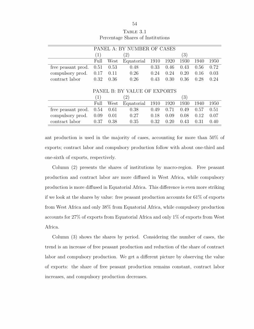
54
Table 3.1Percentage Shares of Institutions
PANEL A: BY NUMBER OF CASES(1) (2) (3)Full West Equatorial 1910 1920 1930 1940 1950
free peasant prod. 0.51 0.53 0.48 0.33 0.46 0.43 0.56 0.72compulsory prod. 0.17 0.11 0.26 0.24 0.24 0.20 0.16 0.03contract labor 0.32 0.36 0.26 0.43 0.30 0.36 0.28 0.24
PANEL B: BY VALUE OF EXPORTS(1) (2) (3)Full West Equatorial 1910 1920 1930 1940 1950
free peasant prod. 0.54 0.61 0.38 0.49 0.71 0.49 0.57 0.51compulsory prod. 0.09 0.01 0.27 0.18 0.09 0.08 0.12 0.07contract labor 0.37 0.38 0.35 0.32 0.20 0.43 0.31 0.40
ant production is used in the majority of cases, accounting for more than 50% of
exports; contract labor and compulsory production follow with about one-third and
one-sixth of exports, respectively.
Column (2) presents the shares of institutions by macro-region. Free peasant
production and contract labor are more diffused in West Africa, while compulsory
production is more diffused in Equatorial Africa. This difference is even more striking
if we look at the shares by value: free peasant production accounts for 61% of exports
from West Africa and only 38% from Equatorial Africa, while compulsory production
accounts for 27% of exports from Equatorial Africa and only 1% of exports from West
Africa.
Column (3) shows the shares by period. Considering the number of cases, the
trend is an increase of free peasant production and reduction of the share of contract
labor and compulsory production. We get a different picture by observing the value
of exports: the share of free peasant production remains constant, contract labor
increases, and compulsory production decreases.

55
3.3.2 Empirical Analysis
In this section, I analyze more in detail the relationship between crops and institu-
tions. Table 3.2 shows the shares of observations for each institution, by crop. There
are groups of crops that are clearly associated with one particular institution. Seven
out of nine crops have about 75% of their observations associated with one only in-
stitution. Cotton is associated with compulsory production; palm kernel and peanuts
with free peasant production; timber, bananas, and coffee with contract labor. Only
cocoa and rubber are not clearly associated with any institution.
Table 3.2Share of Institutions, by Crop (Number of Cases)
compulsory production contract labor free peasant Nbananas 0.00 1.00 0.00 14cocoa 0.23 0.27 0.50 26coffee 0.00 0.74 0.26 31cotton 0.77 0.05 0.18 44palm kernel 0.00 0.00 1.00 44palm oil 0.00 0.00 1.00 41peanut 0.00 0.00 1.00 47rubber 0.32 0.57 0.11 46timber 0.00 1.00 0.00 32all commodities 0.17 0.32 0.51 325
In Table 3.3 I check whether the association between crops and institution dis-
appears if we consider the value of exports instead of the number of observations.
Overall, the strong relationship between groups of crops and institutions is confirmed:
most of the exports for each crop are generated using one only institution.
In Table 3.4, I perform the same analysis, computing the share of exports by
institution for each colony. As for crops, there are some colonies that are clearly
associated with one specific institution. However, only 5 colonies out of 13 produce
more than 75% of their exports with one only institution.
Overall, the relationship between institutions and colonies seems weaker than
the relationship between institutions and crops. It is also possible that a colony

56
Table 3.3Share of Institutions, by Crop (Value of Exports)
compulsory prod. contract labor free peasant 000s francsbananas 0.00 1.00 0.00 81,340cocoa 0.01 0.13 0.86 273,098coffee 0.00 0.90 0.10 289,518cotton 0.86 0.01 0.13 118,663palm kernel 0.00 0.00 1.00 124,182palm oil 0.00 0.00 1.00 60,367peanut 0.00 0.00 1.00 393,831rubber 0.34 0.62 0.04 131,050timber 0.00 1.00 0.00 127,407all commodities 0.09 0.37 0.54 1,599,456
Table 3.4Share of Institutions, by Colony (Value of Exports)
compulsory prod. contract labor free peasant 000s francsCameroon 0.04 0.35 0.61 262,435Chad 0.99 0.00 0.01 49,714Congo 0.39 0.38 0.23 64,637Dahomey 0.03 0.03 0.94 95,632Gabon 0.15 0.75 0.10 60,967Guinea 0.00 0.70 0.30 113,336Haut-Senegal 0.02 0.64 0.34 11,456Haute-Volta 0.00 0.01 0.99 2,230Cote d’Ivoire 0.01 0.67 0.32 447,827Niger 0.01 0.02 0.97 45,651Senegal 0.01 0.05 0.94 341,854Togo 0.11 0.17 0.72 51,645Ubangi-Shari 0.75 0.20 0.05 52,073all colonies 0.09 0.37 0.54 1,599,457

57
is associated with one institution just because it is specialized in the crop that is
associated with that institution. To tackle this issue, I run a series of regressions
including at the same time both crop and colony fixed effects. I run the following
Yijt = α + CROPSβ + COLONIESγ + TIMEδ + εijt (3.1)
where CROPS is a vector of crop fixed effects, COLONIES is a vector of colony
fixed effects, TIME is a vector of time fixed effects.
Table 3.5 shows the results. Panel A reports the results with a dummy variable
for free peasant production as dependent variable. Column (1) shows the results for
crop fixed effects alone: they explain 71% of the variance and they are jointly very
significant, as shown by the F-statistics. Column (2) reports the results for colony
fixed effects alone: they explain only 4% of the variance and, according to the F-test,
they are not significant. In column (3) I include both colony and crop fixed effects;
in column (4) I include crop and time fixed effects; in column (5) I consider all fixed
effects at the same time. In all regressions the main result remains the same: crop
fixed effects account for a very high proportion of the variance and are statistically
significant, while colony and time fixed effects add little explanatory power. In column
(6), I exclude crop fixed effects from the regression: as expected, the R-squared falls
from 78% to 11%.
Panel B reports the results for compulsory production. Crop fixed effects account
for less of the variance (51%), but the main results are qualitatively similar. Panel
C, with contract labor as dependent variable, generates similar conclusions.
In Table 3.6, I check whether the results are driven by particularly small or big
observations. To do so, I exclude from the sample all observations with value of ex-
ports below the 10th and above the 90th percentile. For any institution, the variance
explained by crops (column 1) is much higher than the variance explained by colonies

58
Table 3.5Crops or Colonies?
PANEL ADependent variable is free peasant production
(1) (2) (3) (4) (5) (6)Crop FE Yes No Yes Yes Yes NoColony FE No Yes Yes No Yes YesTime FE No No No Yes Yes YesR2 0.71 0.04 0.73 0.76 0.78 0.11F-crops 167.80*** n/a 595.64*** 331.65*** 260.64*** n/aF-colonies n/a 1.38 1.88* n/a 2.15** 1.27
PANEL BDependent variable is compulsory production
(1) (2) (3) (4) (5) (6)Crop FE Yes No Yes Yes Yes NoColony FE No Yes Yes No Yes YesTime FE No No No Yes Yes YesR2 0.51 0.10 0.57 0.54 0.61 0.16F-crops 58.23*** n/a 21.28*** 26.24*** 24.34 n/aF-colonies n/a 6.83*** 3.40*** n/a 3.95*** 5.15***
PANEL CDependent variable is contract labor
(1) (2) (3) (4) (5) (6)Crop FE Yes No Yes Yes Yes NoColony FE No Yes Yes No Yes YesTime FE No No No Yes Yes YesR2 0.66 0.07 0.69 0.68 0.70 0.08F-crops 39.04*** n/a 376.98*** 1340.26*** 20.78*** n/aF-colonies n/a 13.51** 3.70*** n/a 1.00 7.17***
*** p<0.01, ** p<0.05, * p<0.1. Robust standard errors. N=325

59
(column 2).
Table 3.6Crops or Colonies? Dropping Extreme Observations
PANEL ADependent variable is free peasant production
(1) (2) (3) (4) (5) (6)Crop FE Yes No Yes Yes Yes NoColony FE No Yes Yes No Yes YesTime FE No No No Yes Yes YesR2 0.68 0.08 0.71 0.76 0.77 0.17F-crops 10.24*** n/a 293.74*** 187.83*** 149.77*** n/aF-colony n/a 21.37*** 1.63* n/a 1.79* 2.37***
PANEL BDependent variable is compulsory production
(1) (2) (3) (4) (5) (6)Crop FE Yes No Yes Yes Yes NoColony FE No Yes Yes No Yes YesTime FE No No No Yes Yes YesR2 0.46 0.09 0.53 0.51 0.60 0.16F-crops 41.73*** n/a 15.73*** 21.04*** 19.89*** n/aF-colony n/a 6.21*** 3.23*** n/a 4.22*** 4.92***
PANEL CDependent variable is contract labor
(1) (2) (3) (4) (5) (6)Crop FE Yes No Yes Yes Yes NoColony FE No Yes Yes No Yes YesTime FE No No No Yes Yes YesR2 0.61 0.09 0.66 0.63 0.67 0.09F-crops 32.60*** n/a 184.67*** 950.29*** 158.49*** n/aF-colony n/a 10.67*** 3.39*** n/a 2.93*** 5.02
*** p<0.01, ** p<0.05, * p<0.1. N=260. Robust standard errors.
We observe a strong relationship between crops and institutions. However, it is
also possible that institutions are assigned by exogenous administrative decisions and
that the colonizers choose then the crops that are more suitable for those institutions.
Nevertheless, if this were the case we should observe much bigger colony fixed effects.
Moreover, the historical evidence supports the view that crops affects institutions. For

60
example, poll taxes were introduced in Equatorial Africa to facilitate the collection
of rubber for the concessionary companies and compulsory quotas were established
in Ubangi-Shari in order to increase cotton production.
Finally, it is interesting to note that the explanatory power of settler mortality
is limited. In Table 3.7 I check how much of the variance of institutions can be
explained by (Acemoglu et al., 2001) settler mortality, a factor related to colonies
and not crops. To do so, I simply regress a dummy variable for each institution on
the log of settler mortality from the appendix of (Acemoglu et al., 2001). In none
of the cases we are able to reject the null of no effect of settler mortality on labor
institutions. At least concerning labor institutions in French Africa, settler mortality
does not explain institutions. Overall, the evidence suggests that crops are more
important than colonies in determining labor institutions.
Table 3.7Settler mortality and Labor Institutions
free peasant prod. compulsory prod. contract laborln(settler mortality) -0.029 0.007 0.022
(0.046) (0.038) (0.044)R2 0.002 0.000 0.001F-stat 0.40 0.03 0.26N 255 255 255
Chad, Dahomey and Ubangi-Shari are excluded since they miss settler mortality data.
Robust standard errors are reported in parenthesis.
3.4 What is Behind Crop Fixed Effects?
Crops account for a large portion of the variance in institutions, but they do not
explain the choice of institutions. In this section I explore which factors could be
behind the crops fixed effects, by developing a theoretical model and by providing
some quantitative evidence.

61
3.4.1 Theoretical Framework
Model
There are two agents: Europeans and Africans. The Europeans make profit by
buying or producing crops in Africa and reselling them at higher prices in Europe.
They decide whether to leave the production to Africans (peasant agriculture) or to
establish plantations. If they decide to establish plantations, they use contract labor
to procure the workers they need.8 If the production is left to Africans, the Europeans
can choose between two institutional arrangements: free peasant production or com-
pulsory production. If the free peasant production is chosen, Africans decide whether
to produce cash crops for the colonizers or to stay in the native economy. If compul-
sory production is chosen, the Africans have to provide the established quantity at a
price fixed by the colonizers.
The total population is L. The only input for production is labor l and production
functions are y = E(l) in the European sector (plantation or peasant agriculture) and
N(L − l) in the native economy. All production functions are increasing and non-
convex. The costs for Europeans of the different institutional arrangements are the
following: F (y) increasing with F (0) > 0 if they use contract labor; Q(y) increasing
with Q(0) > 0 if they use compulsory cultivation; pAE(l) if they use , where pA is the
price paid to Africans for production.9
If the Europeans use free peasant production, the price pA is determined in equi-
librium. In particular it is such that the marginal utility of labor for Africans is
the same in the native economy and in the peasant agriculture sector. That is
pA = N ′(L− l)/E ′(l).
The Europeans choose l to maximize their profit under each of the three institu-
8The level of compulsion under contract labor varies. Formally, Africans work for the colonizersfor a wage f ∈ [0, w], where 0 is the wage when contract labor is equal to forced labor and w is thefree labor wage.
9These costs include the cost of collecting the produce or recruiting the workers, monitoring costs,and enforcement costs.
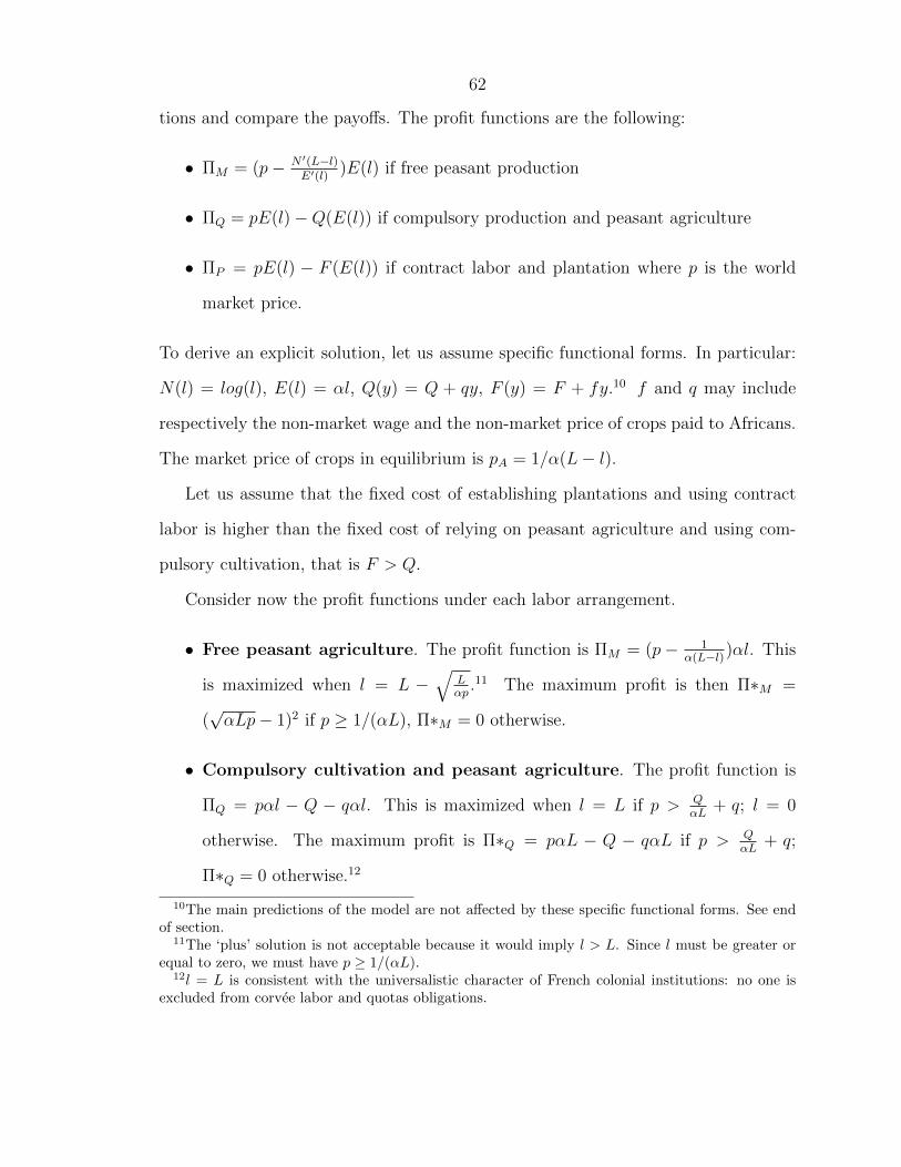
62
tions and compare the payoffs. The profit functions are the following:
• ΠM = (p− N ′(L−l)E′(l)
)E(l) if free peasant production
• ΠQ = pE(l)−Q(E(l)) if compulsory production and peasant agriculture
• ΠP = pE(l) − F (E(l)) if contract labor and plantation where p is the world
market price.
To derive an explicit solution, let us assume specific functional forms. In particular:
N(l) = log(l), E(l) = αl, Q(y) = Q + qy, F (y) = F + fy.10 f and q may include
respectively the non-market wage and the non-market price of crops paid to Africans.
The market price of crops in equilibrium is pA = 1/α(L− l).
Let us assume that the fixed cost of establishing plantations and using contract
labor is higher than the fixed cost of relying on peasant agriculture and using com-
pulsory cultivation, that is F > Q.
Consider now the profit functions under each labor arrangement.
• Free peasant agriculture. The profit function is ΠM = (p− 1α(L−l))αl. This
is maximized when l = L −√
Lαp
.11 The maximum profit is then Π∗M =
(√αLp− 1)2 if p ≥ 1/(αL), Π∗M = 0 otherwise.
• Compulsory cultivation and peasant agriculture. The profit function is
ΠQ = pαl − Q − qαl. This is maximized when l = L if p > QαL
+ q; l = 0
otherwise. The maximum profit is Π∗Q = pαL − Q − qαL if p > QαL
+ q;
Π∗Q = 0 otherwise.12
10The main predictions of the model are not affected by these specific functional forms. See endof section.
11The ‘plus’ solution is not acceptable because it would imply l > L. Since l must be greater orequal to zero, we must have p ≥ 1/(αL).
12l = L is consistent with the universalistic character of French colonial institutions: no one isexcluded from corvee labor and quotas obligations.

63
• Contract labor and plantation. The profit function is ΠP = pαl−F − fαl.
This is maximized when l = L if p > FαL
+ f ; l = 0 otherwise. The maximum
profit is then Π∗P = pαL− F − fαL if p > FαL
+ f ; Π∗P = 0 otherwise.
The following proposition defines the choice of the colonizer.
Proposition 1 The colonizer chooses the following institutions:
• free peasant production, if the price is low, 1/(αL) < p < min{
(1+F+fαL)2
4αL, (1+Q+qαL)2
4αL
}.
• compulsory production, if the price is high and either the marginal cost of
compulsory production or the scale of production are low. In particular if
p > (1+Q+qαL)2
4αLand q < f or if p > (1+Q+qαL)2
4αL, q > f , and αL < F−Q
q−f .
• contract labor, if the price is high and both marginal cost of compulsory produc-
tion and scale of production are high. In particular if p > (1+F+fαL)2
4αL, q > f ,
and αL > F−Qq−f .
• no production, otherwise.
Proof. Compare the maximized profits for each of the three institutions. The profit
from free peasant production is higher than the profit from contract labor if p <
(1+F+fαL)2
4αLand higher than the profit from compulsory production if p < (1+Q+qαL)2
4αL.
The profit of contract labor is higher than the profit of compulsory production when
q > f and αL > F−Qq−f .
The profit of compulsory production is higher than the profit of contract labor
when q < f or when q > f and αL < F−Qq−f . Moreover, notice that (1+Q+qαL)2
4αL> Q
αL+q:
if the profit from compulsory production is higher than the profit from free peas-
ant production , then the profit from compulsory production is positive. Similarly
(1+F+fαL)2
4αL> F
αL+ f : if the profit from contract labor is higher than the profit from
free peasant production, then the profit from contract labor is positive �

64
Notice that the proposition is true in the most general case. As long as the
marginal productivity of labor is decreasing in the indigenous sector, free peasant
production is chosen only when the price is low. When the price is high:
• compulsory production is chosen when F (0) > Q(0) and F ′(.) > Q′(.), or when
Q(0) > F (0), Q′(.) < F ′(.), and production is high;
• contract labor is chosen when Q(0) > F (0) and Q′(.) > F ′(.), or when F (0) >
Q(0), F ′(.) < Q′(.), and production is high.
In the next subsection, I provide the intuition for these results.
Intuition Figure 3.1 shows the choice of institution for a given crop as a function
of the colony’s total productive capacity αL and prices p in each of the two possible
cases: f < q or f ≥ q.13 Green regions represent contract labor/plantation, yellow
regions represent compulsory cultivation/peasant agriculture, red regions represent
free peasant production, white regions represent absence of production.
Effect of price (p). Given the decreasing productivity of labor in the indigenous
economy, the marginal cost of labor under free peasant production is increasing.
For this reason, when the colonizers use free peasant production they do not use
the whole labor force of the colony. On the other hand, under contract labor and
compulsory production all the labor force is employed since the cost of labor is linear.
Thus, an increase in price increases the colonizer’s revenue more under contract labor
/compulsory production than under free peasant production .
If the price of the crop is low, then the total revenue from the colony is not enough
to pay for the fixed costs of compulsory production or plantation. Free peasant pro-
duction is chosen. As the price increases, the revenue from free peasant production
increases less than the revenue from the other two institutions. At a certain price,
13The values of parameters F and Q are 10 when low and 20 when high; the values of parametersf and q are 4 when low and 8 when high; α = 1.

65
Figure 3.1Institutional regions

66
the revenue is high enough to compensate the fix cost and contract labor/compulsory
production is chosen.
Effect of scale of production (αL). The fixed cost of establishing a planta-
tion is higher than that of establishing compulsory cultivation (F > Q). Thus, in
places where the cost of an additional unit is higher under contract labor than under
compulsory production (f > q), the colonizer will only choose between compulsory
production and free peasant production. This is the situation of panel A of figure 3.1.
In places where the cost of an additional unit is higher under compulsory pro-
duction than under contract labor (q > f), when the scale of production increases
enough contract labor becomes more attractive than compulsory production, as shown
in panel B of figure 3.1.
3.4.2 Testable Implications and Evidence
The model yields the following predictions about the effects of scale of production
and prices.
1. H1. Price. In colony/crops where the price of crop is low, we should observe
only free peasant production.
2. H2. Scale of production. Colony/crops that use contract labor have higher
scale of productions than those that use compulsory production cultivation.
I perform the following tests.
1. To test H1, I regress a dummy for free peasant production on price, controlling
for quantity.14 I expect a negative coefficient.
2. To test H2, I restrict the sample to contract labor and compulsory production
14I need to control for quantity because the model predicts free peasant production when p <
min{
(1+F+fαL)2
4αL , (1+Q+qαL)2
4αL
}= min
{(1+F+fY )2
4Y , (1+Q+qY )2
4Y
}.

67
and I regress a dummy for contract labor on the total quantity produced. I
expect a positive coefficient.
Table 3.8 reports the results. Panel A tests H1. As expected, there is a negative and
significant relation between the price of crops and the use of free peasant production:
a standard deviation increase in price decreases the probability of free peasant pro-
duction by 16 percentage points. As shown in columns (2) to (4) this relationship is
robust to the inclusion of colony, time, and crop fixed effects. As expected, since we
are looking for which factors are behind the crop fixed effects, when we include crop
fixed effects the coefficient of price drops. Crops explain, in fact, more than 40% of
the variance in price.15
Panel B tests H2. As expected, the coefficient of quantity is positive and sig-
nificant: a larger scale of production is associated with more contract labor and
less compulsory cultivation. A standard deviation increase in quantity increases the
probability of contract labor vs. compulsory production by 10 percentage points. The
relationship is robust to the inclusion of colony and time fixed effects (columns 2 and
4). However, the coefficient of quantity becomes insignificant when we control for the
kind of crops (column 4).
Overall, prices seem to be important in determining the choice between market
and non-market institutions, while the scale of production has explanatory power for
the choice between compulsory production and contract labor.
3.5 Conclusion
The main theories attributing African underdevelopment to extractive institutions
established by colonizers explain the origin of these policies with factors that are
15The high explanatory power that crop fixed effects still have can be explained by the fact thatthe test assumes common costs of production (Q and q, F and f) for all colonies, crop, and periods.Thus, when we observe free peasant production we cannot be sure if it is because the price p is lowor because the costs of production Q and q are high.

68
Table 3.8Testing the Effects of Price and Scale of Production
PANEL Afree peasant
(1) (2) (3) (4)price net of trading costs -0.0597*** -0.0571*** -0.0582*** -0.0135**
(0.00662) (0.00708) (0.0086) (0.00662)quantity -0.000314 -0.000253 -0.00067 0.000122
(0.000797) (0.000755) (0.000865) (0.000156)Colony FE YesTime FE yesCrop FE YesN 325 325 325 325R2 0.094 0.125 0.145 0.714
PANEL Bcontract labor
(1) (2) (3) (4)quantity 0.00264*** 0.00252*** 0.00203*** 0.000137
(0.000615) (0.000669) (0.000547) (0.000126)Colony FE YesTime FE yesCrop FE YesN 159 159 159 159R2 0.041 0.252 0.061 0.593

69
colony-specific, such as settler mortality (Acemoglu et al., 2001). However, the precise
details are not clear and the origin of extractive institutions remains a black box. In
this chapter, I contribute to this literature, by focusing on the determinants of labor
institutions in the French colonies.
By using a dataset of labor institution, I find that the relationship between colonies
and institutions is much weaker than expected. On the other hand, I show that there
exists a strong correlation between labor institutions and kind of crops and that this
relationship takes into account most of the variation in labor arrangements. This
evidence suggests that factors related to crops, such as prices, are more likely to
explain labor institutions than factors related to colonies, such as settler mortality.
To interpret these findings, I develop and test a theoretical model, linking the choice
of labor arrangements to differences in price of crops, cost of institutions, and scale
of production. The results suggest that these variables are key factors explaining the
correlation between crops and institutions.
3.6 Appendix
3.6.1 Definition and Sources
See appendix 2.8.3.
3.6.2 Appendix Figures and Tables

70
Table3.9
Sum
mar
ySta
tist
ics
Vari
able
Obs
Mean
Std
.D
ev.
Min
Max
com
puls
ory
pro
duct
ion
325
0.16
90.
375
01
contr
act
lab
or32
50.
320
0.46
70
1fr
eep
easa
nt
pro
duct
ion
325
0.51
10.
501
01
equat
oria
l32
50.
403
0.49
10
1quan
tity
(ton
s)32
512
340
3525
610
2815
04pri
ceF
rance
net
oftr
adin
gco
sts
(per
kg)
325
1.30
2.58
0.01
17.9
1pri
ceA
fric
a(p
erkg)
325
0.75
1.27
0.01
9.30

71
Chapter 4
Colonial Institutions, Prices to
Producers, and Current African
Development
4.1 Introduction
Since early 2000s, a growing body of studies has pointed to institutions as one of the
main causes of African underdevelopment. One line of research emphasizes colonial
institutions at the national level, blaming in particular their extractive character and
the low level of property rights protection (Acemoglu et al., 2001). A second line of
research focuses instead on pre-colonial conditions at the local level, affected by the
slave trade (Nunn and Wantchekon, 2011) and the political centralization of ethnic
institutions (Michalopoulos and Papaioannou, 2013).
This chapter connects these two literatures, by exploring the relationship between
colonial extraction at the local level and current development.1 Measuring colonial
1Recent works have emphasized how local features of colonial rule, such as investments in ed-ucation (Huillery (2009) and Cogneau and Moradi (2014)), arbitrary borders (Michalopoulos andPapaioannou, 2013), and missionary activity (Nunn, 2010) affect current development.

72
extraction, in particular at the sub-national level, is challenging for lack of data and
absence of clear counterfactuals. Since colonial extractive institutions were used in
all colonies, we cannot observe subsequent development in the absence of extraction.
To solve these problems, I exploit the peculiar structure of trade and labor policies
employed by the French colonizers. In French Sub-Saharan Africa, trade monopsonies
and forced labor were introduced to reduce prices to African agricultural producers
and increase the profit margin of the European trading companies. The gap between
observed prices and theoretical “free market” prices can thus be used as a proxy for the
extent of colonial extraction. Using data collected in the French colonial archives, I
compute colony-level price gaps for the main crops produced, as the difference between
prices to producers and prices in France net of trading costs. Then, I combine the
gaps for each crop/colony with GIS data on crop suitability in order to construct
price gaps at the sub-national level.
I show that price gaps are strongly negatively correlated with current development,
as proxied by luminosity data from satellite images (Michalopoulos and Papaioannou,
2013). The relationship is not driven by observable differences in land endowments,
geography, disease environment, resources, population density, urbanization, or access
to markets. Neither, it is driven by pre-existing differences in economic development
during the colonial period, as proxied by the value of agricultural production in 1950s.
Moreover, the correlation is robust to the inclusion of country fixed effects: colonial
price gaps account for differences in development both across and within countries.
Finally, the negative relationship between price gaps and development is not only
statistically significant, but also economically meaningful: for a median district, one
standard deviation increase in the price gaps is associated with a 10 to 30% decrease
in luminosity.
I then explore the channels which mediate the relationship between colonial price
gaps and current economic development, by looking at luminosity in urban and rural

73
areas. I show that price gaps are negatively correlated with size of urban areas and
level of development in rural areas. Interestingly, the relationship between price gaps
and development in urban areas is instead positive. The overall impact is negative, but
colonial extraction benefited cities, increasing the urban-rural development gap. The
economic benefits that urban sectors of society obtained can be the reason why trade
monopsonies and extractive institutions persisted long after independence, despite
their negative influence on overall development.
The chapter is structured as follows. Section 4.2 presents the historical background
and discusses price gaps and luminosity data. Section 4.3 shows the results of the
empirical analysis, both across and within countries. Section 4.4 focuses on potential
channels of causality. Section 4.5 provides concluding remarks and directions for
future research.
4.2 Historical Background and Data
About one-third of Sub-Saharan Africa and one-fifth of its population was subject
to French colonization between 1880 and 1960. Compared to the neighboring British
colonies, the French territories were much poorer. For this reason, the colonizers, in-
stead of focusing on productive investments, limited themselves to trade with African
populations. Trading companies bought agricultural production at low prices from
African producers and resold it at higher prices in Europe. However, since popula-
tion density was low and labor expensive, the market price of crops was too high,
eliminating in this way any profit for the trading companies.
In order to maintain profits, the companies lobbied the colonial government to
establish trade monopsonies and specific labor institution. If trade monopsonies were
common to almost all colonies (fewer than a dozen companies monopolized all trade
from West Africa), labor institutions varied across colonies, crops, and over time.

74
They ranged from free labor, as in the case of peanuts production in Senegal, to
compulsory cultivations, as in the case of cotton in Ubangi-Shari or rubber in Congo.
Tadei (2013) shows that monopsonies and coercive labor institutions proved ex-
tremely effective in allowing the colonizers to pay African producers prices far below
world market prices, cutting African gains from trade by over 60% during the colo-
nial period. With independence coercive labor institutions were abolished, but trad-
ing monopsonies tended to persist, and post-independence governments continued to
practice price policies that discriminated against agricultural producers.
4.2.1 Price Gaps
A way to measure how much prices to producers were reduced is to compare them
to counterfactual prices under competition among trading firms and free labor. The
idea is that without monopsonies and labor coercion the price to producers should
be equal to the world market prices net of trading costs. To do so, I construct the
following price gap index
G = 1− pA − tp− T − t
(4.1)
where pA is the price at the African port, p is the price in France, t are inland transport
costs between the interior of the interior of the colony and the port, and T includes
shipping and fixed costs.
I collect yearly data on prices in Africa and in France for each crop in 1950s from
colonial custom statistics 2. To take into account price shocks in specific years (e.g.,
fluctuation of supply due to climatic conditions), I use the average of prices across
all the years in the 1950s for each crop/colony. Moreover, since data for the various
crop/colonies might come from different years, I compute the average price in France
in 1950s for each crop and I recompute prices at the African ports proportionally.
2See Tadei (2013) for detailed information about the sources. Prices in Africa are measured atthe port also for landlocked colonies. In fact, prices for the same crop are not significantly differentfor coastal and landlocked colonies. See table 4.7 in the Appendix.
75
I estimate shipping and fixed costs according to the procedure described in 2 and
I compute inland transport costs by using colonial maps and reports. To do so, I
first put together a map of current ports, rivers, and railroads. Then, I eliminate all
railroads segments that were constructed after independence, all portions of rivers
that were not navigable, and all ports that were not used during the colonial period,
by using a map of colonial transports in French Africa in 1956 (Duignan and Gahan,
1975, p.149, vol.4) and the accounts in Suret-Canale (1971) and Thomas (1957).
Figure 4.1 represents the final colonial transport network map. According to Thomas
(1957), four ports (Dakar, Conakry, Abidjan, and Cotonou) handled 95% of all the
trade from French West Africa and 75% of exports were moved to ports via railroads.
Finally, by using information from a variety of colonial reports (see Data Appendix),
I construct estimates of the cost per km for each mean of transport (railroad, river,
and roads) and with GIS I compute the total cost from the centroid of each district
to the closest port, along the cheapest route.3
Colonial data on prices are aggregated at the commodity/colony level. To con-
struct a price gap index specific for each district, I combine colonial prices with data
on crop suitability from the FAO Global Agro-Ecological Zones project, which reports
potential productivity (kg/hectare) for each crop globally at a 5 by 5 km resolution,
given climatic and soil constraints and input levels (FAO, 2013b). I proceed in the
following way:
1. First, I compute a crop/pixel-level price gap for each crop. A crop is considered
to be produced in the pixel if colonial data report non-null production in the
colony in which the pixel is located and if inland transport costs from the pixel
district to the port are lower than the reported price at the port. I focus
the analysis on four agricultural commodities: cocoa, cotton, palm kernel, and
peanut, accounting for over half of the total value of exports from French Africa.
3I connect the centroids of districts to the railroad/ rivers networks, by using a 50 km by 50 kmgrid of “roads”.

76
Figure 4.1Transportation Network in Colonial French Africa, 1950s
The figure represents the transportation network of French Africa during the colonial period, in-
cluding railroads (black), navigable rivers (blue), and main ports (dark blue). The green dots are
the centroid of each district.

77
These crops were produced by African peasants, unlike coffee or bananas that
were produced under European plantation. For this reason, the price in Africa
does not include the profit of the European planter and it is a better measure
of the income of African producers.
2. Second, I compute a pixel-level price gap, by averaging the crop/pixel-level
gaps weighted by each crop’s value per hectare (price to African producer times
productivity) in the given pixel. The underlying idea is that the land in each
pixel is assigned to each crop in proportion to its value.
3. Finally, by using GIS, I compute a district-level price gap as the average of pixel-
level price gaps within each districts. I consider second-level administrative
divisions of 13 ex-French colonies, adding up to 539 districts. Districts that did
not produce any of the four crops are excluded.
4.2.2 Luminosity
As a proxy for local economic development, I employ luminosity data from satellite
images of the world at night. The use of luminosity as measure of development builds
on the work of Michalopoulos and Papaioannou (2013). Given the high correlation
with wealth, electrification, and schooling, they show that light density at night is
particularly useful as a proxy for economic activity in areas where no other local-level
measures are widely available, such in the case of Sub-Saharan Africa.
The data come from the Earth Observation Group of the NOAA National Geo-
physical Data Center (2013) which reports the intensity of light radiation at a 15
arc-sec resolution (about 500 square meters) for the entire globe. This measure
uses cloud-free observations in 2012/4/18-26 and 2012/10/11-23 and includes elec-
tric lights, fires, and gas flares. The unit of measurement is nano-Watts/(cm2*sr).
To construct my development measure at the district level, I average pixel-level lu-

78
minosity at the desired level of aggregation by using GIS.
4.3 Colonial Price Gaps and Current Development
Before formally exploring the relationship between price gaps and luminosity, let us
observe some preliminary evidence. Figure 4.2 represents French Sub-Saharan Africa.
The red area is the focus of the analysis, including all districts in which at least one
crop was produced, among cocoa, cotton, palm kernel, or peanut.
Figure 4.2French Africa and Area of Analysis
The figure represents French Sub-Saharan Africa, excluding Madagascar and Djibouti. The analysis
is focused on the districts in the red area, where it was produced at least one of the four crops
considered (cocoa, cotton, peanut, palm kernel).
Figure 4.3 shows the average price gaps and luminosity for each district. It is easy
to notice a negative correlation between the two variables On average, districts below
the median price gap are about 45% brighter than districts above the median (0.26

79
Figure 4.3Average Current Luminosity and Colonial Price Gap by District
The top and bottom panel report the average luminosity the average colonial price gap and in each
district, respectively. Districts are color-coded according to five quantiles.
vs. 0.18).
Figure 4.4 shows the relationship between log(light) and log (price gap). I use logs
to reduce the impact of extreme value observations and to have a more direct interpre-
tation of regression coefficients as elasticities.4 The top panel shows the relationship
within the full sample: the presence of a negative correlation is evident. This rela-
tionship is not driven by the presence of cities or outliers, as it is even stronger when
excluding districts with luminosity values higher than the 90th percentile (bottom
panel).
To formally analyze the correlation between lights and price gaps, I run the fol-
4Kernel densities in figure 4.7 shows that the log of the variable follow more closely a normaldistribution.

80
(a) Full Sample
(b) Excluding +90 Percentile of Luminosity
Figure 4.4Colonial Price Gaps and Current Luminosity
The top panel reports the scatterplot and the linear fitting for the regression of log (light) and log
(price gap) for the full sample. In the bottom panel I exclude district with luminosity higher than
the 90th percentile, in order to control for outliers and the presence of cities.

81
lowing regression
log(Li) = α0 + αi + βlog(Gi) +Xiγ + εi (4.2)
where log(Li) is the natural logarithm of the average luminosity in district i, log(Gi)
is the natural log of price gap, Xi is a vector of control variables, αi are country fixed
effects (used in some specifications), α0 is a constant, and εi is the error term. Since
price data are at the colony level, I cluster standard errors at the country level. All
variables are averages of the values per pixel within each district.
Control variables include a variety of geographic, economic, and ecological factors,
such as the percentage of land covered by forest, desert, and water, the percentage
of cultivated land, elevation, malaria suitability index, livestock, value of agricultural
production, population density, distance to port, and presence of oil. These controls
are important for several reasons. First, controlling for the presence of forest allows
us to take into account the impact on development of wood exports, particularly
large in Gabon and Congo. The percentage of land covered by desert and water is
useful to control for the blooming of satellite light images due to deserts and water
bodies. Including the percentage of cultivated land allows us to control both for
the presence of unproductive land and for urbanization. Elevation is important as
Nunn and Puga (2012) show that ruggedness of the terrain is negatively related to
slave exports and Michalopoulos (2012) demonstrates that variability in elevation is
positively correlated with ethnic fractionalization. The inclusion of the malaria index
is warranted by several studies showing the impact of malaria and disease environment
on development (Gallup and Sachs, 2001). Livestock allows us to control for an
important source of income in countries less suitable to agriculture such as Mali,
Niger, and Chad, while the value of agricultural production accounts for variations
in land suitability and crop endowments. Population density is a common proxy
for economic development, accounts for urbanization, and reflects the availability of
labor. The distance to the port is included to take into account variations in the

82
access to world markets. Finally, it is important to control for oil both for its positive
impact of income and negative impact on the quality of institutions
Table 4.1 reports the OLS cross-sectional estimates, without country fixed effects.
The simple regression of log (light) on log (price gap) is shown in column (1). The
coefficient is negative and statistically significant at 1% level. In column (2) I con-
trol for geographic characteristics and land cover, including the percentage of land
covered by forest, desert, and water, the percentage of cultivated land, elevation, and
a malaria suitability index. In column (3) I condition on resources characteristics
and access to markets, by including a measure of livestock, the log of the average
value of current agricultural production, population density, linear distance to the
closest port, and a dummy for districts with oil. Column (4) reports the results
controlling for both geography and resources.5 Despite this rich set of controls, in
all specifications, the coefficient of price gap, even if decreases a little in absolute
value, remain negative and highly significant. In the specification with all control
variables, elevation, malaria, and livestock have negative and significant coefficients,
while population density enters the specification with a positive coefficient.
5Please see the Data Appendix for detailed definitions and sources for all the variables.

83
Table4.1
Col
onia
lP
rice
Gap
san
dC
urr
ent
Dev
elop
men
t:C
ross
-Sec
tion
alE
stim
ates
(1)
(2)
(3)
(4)
(5)
(6)
(7)
(8)
(9)
(10)
Log
(pri
cega
p)
-0.4
44∗∗
-0.3
64∗∗
-0.3
15∗∗∗
-0.2
90∗∗∗
-0.4
19∗∗
-0.2
76∗∗
-0.3
14∗∗∗
-0.3
12∗∗∗
-0.2
69∗∗∗
-0.3
19∗∗∗
(0.1
46)
(0.1
26)
(0.0
994)
(0.0
820)
(0.1
60)
(0.1
01)
(0.0
721)
(0.0
881)
(0.0
789)
(0.0
812)
Geo
grap
hy
Con
trol
sY
esY
esY
esY
esY
esY
esY
esR
esou
rces
Con
trol
sY
esY
esY
esY
esY
esY
esY
esP
re-c
olon
ial
Sta
teC
entr
aliz
atio
nY
esY
esE
qu
ator
ial
Afr
ica
Du
mm
yY
esE
xcl
ud
ing
Ou
tlie
rsY
esE
xcl
ud
ing
Hig
hL
um
inos
ity
Yes
Excl
ud
ing
Hig
hly
Bu
ilt
Yes
N53
953
953
953
947
847
852
853
951
351
2R
20.
075
0.19
10.
155
0.23
20.
078
0.25
60.
241
0.29
10.
269
0.21
0
Th
eta
ble
rep
orts
OL
Ses
tim
ates
ofth
ere
lati
onsh
ipb
etw
een
colo
nia
lp
rice
gap
san
dcu
rren
td
evel
opm
ent,
asp
roxie
dby
lum
inosi
ty.
Th
esi
mp
lere
gre
ssio
nof
log
(lig
ht)
on
log
(pri
cega
p)
isre
por
ted
inco
lum
n(1
).In
colu
mn
(2)
Ico
ntr
ol
for
geo
grap
hic
char
acte
rist
ics,
incl
ud
ing
the
per
centa
ge
ofla
nd
cove
red
by
fore
st,
des
ert,
and
wat
er,
the
per
centa
ge
ofcu
ltiv
ate
dla
nd,
aver
age
elev
atio
n,
and
am
alar
iasu
itab
ilit
yin
dex
.In
colu
mn
(3)
Ico
ntr
olfo
rre
sou
rces
chara
cter
isti
cs,
by
incl
ud
ing
am
easu
reof
lives
tock
,th
elo
gof
the
aver
age
valu
eof
curr
ent
agri
cult
ura
lp
rod
uct
ion
,p
opu
lati
ond
ensi
ty,
linea
rd
ista
nce
toth
ecl
oses
tp
ort
,an
da
du
mm
yfo
r
dis
tric
tsw
ith
oil
.C
olu
mn
(4)
rep
ort
sth
ere
sult
sco
ntr
olli
ng
for
bot
hge
ogra
phy
and
reso
urc
es.
Inco
lum
n(5
)an
d(6
)I
contr
olfo
rp
re-c
olo
nia
lst
ate
centr
ali
zati
on
,
wit
hou
tan
dw
ith
the
full
set
ofge
ogra
phy
and
reso
urc
esva
riab
les.
Inco
lum
ns
(7)
to(1
0)I
per
form
furt
her
rob
ust
nes
sch
ecks
on
the
spec
ifica
tion
wit
hth
efu
llse
t
ofco
ntr
ols
,by
excl
ud
ing
ou
tlie
rs(7
),ad
din
gan
Equ
ato
rial
Afr
ica
du
mm
y(8
),ex
clu
din
gd
istr
icts
wit
hlu
min
osit
yh
igh
erth
an
the
90t
hp
erce
nti
le(9
)an
dex
clu
din
g
dis
tric
tsh
igh
erth
an
the
90p
erce
nti
lein
bu
ilt-
up
lan
d.
Ple
ase
see
the
Dat
aA
pp
end
ixfo
rd
etail
edd
efin
itio
ns
and
sou
rces
for
all
the
vari
able
s.R
ob
ust
stan
dard
erro
rscl
ust
ered
atth
eco
untr
yle
vel
are
rep
ort
edin
par
enth
esis
.***
p<
10%
,**p<
5%
,*p<
10%
.

84
In column (5) and (6) I control for pre-colonial state centralization, without
and with the full set of geography and resources variables. This control is due to
Michalopoulos and Papaioannou (2013), who shows that the centralization of ethnic
groups in the colonial period is positively correlated to current luminosity. Since
data on pre-colonial institutions are not available for all districts, the sample size is
slightly smaller. However, the coefficient of price gap is unaffected. Interestingly, the
coefficient of pre-colonial centralization is negative, and significant at 10% in the spec-
ification with the full set of controls. This is contrary to the finding in Michalopoulos
and Papaioannou (2013) and could be explained by the “direct rule” style of the
French which may have reduced the importance of pre-colonial institutions.
In columns (7) to (10) I perform further robustness checks on the specification
with the full set of controls, by excluding outliers (7), adding an Equatorial Africa
dummy (8), excluding districts with luminosity higher than the 90th percentile (9)
and excluding districts higher than the 90 percentile in built-up land.6 Controlling
for the percentage of build-up land allows us to make sure that the relationship is not
driven by cities and urbanization. Again, the coefficient of price gap is negative and
significant across all specifications.
The relation between price gaps and development is is not only statistically signif-
icant, but also economically meaningful: a 1% increase in price gap is associated with
a 0.3 % decrease in luminosity. To get a better idea of the intensity, consider that, for
the average district, one standard deviation increase in log(price gap) is associated
with a decrease in log(light) by about 10%.
Table 4.2 reports the results including country fixed effects. In this case, the
coefficient of price gap measures the relationship between price gap and luminosity
within countries. Moreover, adding fixed effects allows us to control for a variety of
country-level characteristics, such as the quality of national institutions. Column (1)
6Outliers are identified using the method in Hadi (1993). The Equatorial dummy is negative andhighly significant.

85
reports the simple fixed-effect regression. The coefficient of log (price gap) is negative
and highly significant, and about three times larger than in the specification without
fixed effect (compare to table 4.1, column 1). In column (2) I control for geographic
characteristics, in column (3) I control for resources, and column (4) conditions on
both geography and resources together. In all specifications, the coefficient of interest
remains negative and significant. In column (5) I control for pre-colonial state cen-
tralization, while in column (6) I include the full set of controls (geography, resources,
and pre-colonial centralization). The coefficient of price gaps decreases, but is still
negative and significant.7
7The coefficients of control variables are generally consistent with the cross-sectional estimates.

86
Table4.2
Col
onia
lP
rice
Gap
san
dC
urr
ent
Dev
elop
men
tW
ithin
Cou
ntr
ies:
Fix
edE
ffec
tsE
stim
ates
(1)
(2)
(3)
(4)
(5)
(6)
Log
(pri
cega
p)
-1.1
23∗∗∗
-0.8
62∗∗
-0.7
75∗∗
-0.6
79∗
-1.0
12∗∗∗
-0.6
37∗
(0.2
94)
(0.3
48)
(0.2
61)
(0.3
41)
(0.3
22)
(0.3
32)
Cou
ntr
yF
ixed
Eff
ects
Yes
Yes
Yes
Yes
Yes
Yes
Geo
grap
hy
Con
trol
sY
esY
esY
esR
esou
rces
Con
trol
sY
esY
esY
esP
re-c
olon
ial
Sta
teC
entr
aliz
atio
nY
esY
es
N53
953
953
953
947
847
8R
20.
096
0.19
50.
150
0.22
80.
112
0.25
7
Th
eta
ble
rep
orts
OL
Ses
tim
ate
sof
the
rela
tion
ship
bet
wee
nco
lon
ial
pri
cegap
san
dcu
rren
td
evel
op
men
t,as
pro
xie
dby
lum
inos
ity,
incl
ud
ing
cou
ntr
yfi
xed
effec
ts.
Th
esi
mp
lere
gre
ssio
nof
log
(lig
ht)
on
log
(pri
cegap
)
isre
por
ted
inco
lum
n(1
).In
colu
mn
(2)
Ico
ntr
ol
for
geo
gra
ph
icch
ara
cter
isti
cs(p
erce
nta
ge
of
lan
dco
ver
ed
by
fore
st,
des
ert,
and
wat
er,
per
centa
ge
of
cult
ivate
dla
nd
,av
erage
elev
ati
on
,an
dm
ala
ria
suit
ab
ilit
yin
dex
)
and
inco
lum
n(3
)I
contr
ol
for
reso
urc
es(l
ives
tock
,lo
gva
lue
of
curr
ent
agri
cult
ura
lp
rod
uct
ion
,p
op
ula
tion
den
sity
,lin
ear
dis
tan
ceto
the
close
stp
ort
,an
doil
du
mm
y).
Colu
mn
(4)
rep
ort
sth
ere
sult
sco
ntr
oll
ing
for
bot
hge
ogra
phy
and
reso
urc
es.
Inco
lum
n(5
)I
contr
ol
for
pre
-colo
nia
lst
ate
centr
ali
zati
on
.In
colu
mn
(6)
Iin
clu
de
the
full
set
ofco
ntr
ols
(geo
gra
phy,
reso
urc
es,
an
dp
re-c
olo
nia
lce
ntr
ali
zati
on
).P
lease
see
the
Data
Ap
pen
dix
for
det
aile
dd
efin
itio
ns
an
dso
urc
esfo
rall
the
vari
ab
les.
Th
eR
2m
easu
res
the
exp
lain
edva
rian
ce
wit
hin
cou
ntr
ies.
Rob
ust
stan
dard
erro
rscl
ust
ered
at
the
cou
ntr
yle
vel
are
rep
ort
edin
pare
nth
esis
.***
p<
10%
,**
p<
5%,
*p<
10%
.

87
Price gaps explain variation in luminosity not only across countries, but also
within the districts of the same country. The magnitude of the fixed effects estimates
is even larger than that of the cross-sectional estimates. For the average district, one
standard deviation increase in log (price gap) is associated with a 30% decrease in
luminosity.
Obviously, despite the large set of control variables employed, we might still be
concerned that the negative relationship between price gaps and development is driven
by omitted variables. For example, if the colonizers reduced prices to producers more
in districts that were already poor in the colonial period and these districts are still
the poorest today, then the observed correlation would be spurious. This might be
the case if poorer districts responded less to price incentives or if the colonizers did
not reduce agricultural prices in rich and highly urbanized districts, where agriculture
was not important.
However, there are reasons to believe that these should not be big concerns. First,
Tadei (2013) shows that price elasticity is uncorrelated with the extent of price re-
duction. Second, the relationship between price gaps and luminosity holds even when
excluding highly urbanized districts and controlling for population density (see table
4.1).
To provide further evidence, I study the relationship between colonial agricultural
production and price gaps. In column (1) of table 4.3 I regress log (price gap) on
the log of the potential value of agricultural production in 1950s. For each pixel
and crop, I estimate the potential value as the product of the price in France net
of trading costs times the productivity per hectare times the cultivated land area.
Then, I compute the value per pixel by weighting each crop by its value and I average
within districts. Using potential instead of actual production has two advantages.
First, it allows us to use the full sample since colonial data on actual production at
the district level are available only for a minority of districts. Second, potential value

88
is not affected by price gaps and we can rule out the possibility of reverse causality.
According to the estimates of column (1), prices are reduced less in richer districts.
Nevertheless, the correlation between potential agricultural production and price gaps
becomes insignificant when including country fixed effects.

89
Table4.3
Col
onia
lA
gric
ult
ura
lP
roduct
ion,
Pri
ceG
aps,
and
Curr
ent
Dev
elop
men
t
Dep
enden
tV
aria
ble
(1)
(2)
(3)
(4)
(5)
(6)
Log
(pri
cega
p)
Log
(pri
cega
p)
Log
(lig
ht)
Log
(lig
ht)
Log
(lig
ht)
Log
(lig
ht)
Log
(pot
enti
alva
lue
1950
s)-0
.092
1∗∗
0.00
289
0.03
790.
103
-0.0
252
0.06
75(0
.033
1)(0
.013
0)(0
.030
3)(0
.065
6)(0
.031
4)(0
.047
6)
Log
(pri
cega
p)
-0.3
91∗∗
-0.2
85∗∗∗
-1.1
19∗∗∗
-0.6
55∗
(0.1
64)
(0.0
883)
(0.2
87)
(0.3
32)
Cou
ntr
yF
ixed
Eff
ects
Yes
Yes
Yes
Geo
grap
hy
Con
trol
sY
esY
esR
esou
rces
Con
trol
sY
esY
es
N53
953
953
953
953
953
9R
20.
127
0.00
00.
082
0.24
10.
098
0.23
1
Th
eta
ble
rep
orts
OL
Ses
tim
ates
ofth
ere
lati
on
ship
bet
wee
nco
lon
ial
agri
cult
ura
lp
rod
uct
ion
an
dp
rice
gap
san
db
etw
een
pri
ceco
lon
ial
pri
cega
ps
and
curr
ent
dev
elop
men
t,as
pro
xie
dby
lum
inosi
ty.
Th
esi
mp
lere
gre
ssio
nof
log
(pri
cegap
)on
the
log
of
the
pote
nti
al
valu
e
ofag
ricu
ltura
lp
rod
uct
ion
in19
50s
isre
port
edin
colu
mn
s(1
)an
d(2
),w
ith
an
dw
ith
ou
tco
untr
yfi
xed
effec
ts.
Inco
lum
ns
(3)
to(6
)I
rep
ort
the
regr
essi
onof
log
(lig
ht)
onlo
g(p
rice
gap
),co
ntr
oll
ing
for
the
valu
eagri
cult
ura
lpro
du
ctio
nin
1950s:
colu
mn
(3)
rep
ort
sth
e
sim
ple
regr
essi
on;
colu
mn
(4)
contr
ols
for
geo
gra
phy
(per
centa
ge
of
lan
dco
vere
dby
fore
st,
des
ert,
an
dw
ate
r,p
erce
nta
ge
of
cult
ivate
d
lan
d,
aver
age
elev
atio
n,
and
mal
aria
suit
ab
ilit
yin
dex
)an
dre
sou
rces
(liv
esto
ck,
log
valu
eof
curr
ent
agri
cult
ura
lp
rod
uct
ion
,p
op
ula
tion
den
sity
,li
nea
rd
ista
nce
toth
ecl
oses
tp
ort
,an
doil
du
mm
y);
colu
mn
(5)
incl
ud
esco
untr
yfi
xed
effec
tsto
the
sim
ple
regre
ssio
n;
colu
mn
(6)
incl
ud
esco
untr
yfi
xed
effec
tsto
the
spec
ifica
tion
wit
hth
efu
llse
tof
contr
ols
.In
the
spec
ifica
tion
sw
ith
fixed
effec
ts,th
eR
2m
easu
res
the
exp
lain
edva
rian
cew
ithin
cou
ntr
ies.
Rob
ust
stan
dard
erro
rscl
ust
ered
at
the
cou
ntr
yle
vel
are
rep
ort
edin
pare
nth
esis
.***
p<
10%
,
**p<
5%,
*p<
10%
.

90
In column (3) to (6) I directly estimate the relationship between price gaps and
lights, including colonial agricultural production as a control variable. Column (3)
reports the simple regression, column (4) controls for geography and resources, col-
umn (5) includes country fixed effects to the simple regression, and column (6) adds
country fixed effects to the specification with the full set of controls. In none of the
specifications the coefficient of agricultural production in 1950s is significant. On the
other hand, the coefficient of price gaps is negative, significant, and of similar mag-
nitude as the specifications without colonial agricultural production (tables 4.1 and
4.2).
4.4 Channels of Causality: Effects on Rural and
Urban Areas
Colonial price gaps are negatively correlated with current development. The relation-
ship is robust to a variety of specifications and cannot be explained by differences
in geography, natural resources, population density, urbanization, and pre-existing
levels of economic development
In this section, I explore the channels through which price gaps might affect sub-
sequent economic growth. A negative relationship between price gaps and average
district luminosity suggests four possible channels of causality. Colonial extraction
may affect current economic growth by reducing
1. the size or the number of cities;
2. the size of rural settlements vs. not-inhabited areas;
3. the level of development in cities, without changing their number or size;
4. the level of development in rural areas (intensive agriculture, capital invest-
ments, machinery), without changing their size.

91
I start by exploring channels 1 and 2. To test whether the effect goes through the size
or the number of cities (channel 1), I consider the share of pixel in each district that
are within the top one percentile of luminosity. The idea is that the most lit pixels are
those belonging to urban areas. Figure 4.5 shows the top percentile pixels together
with the locations of major cities. The relationship is evident: the top percentile is a
good threshold to identify cities.
Figure 4.5Top Percentile Lights and Capitals
The figure shows in red the pixels within the top one percentile and the location of country capitals.
The red area south of Libreville is Lake Nkomi (water areas magnify satellite image luminosity),
while the area west of Brazzaville is the city of Pointe-Noire.
Notice also that the two distributions of light within and below the top percentile
are much closer to normals than the distribution from the full sample (compare the
top panels of figure 4.8 to figure 4.7).8
In table 4.4, I regress the share of top percentile/urban pixels in each district on
price gaps. Column (1) reports the simple regression: the coefficient of price gaps is
negative and significant. Larger price gaps are associated with a lower share of urban
pixels. The result is unchanged if we control for geography, natural resources, and
agricultural production in the colonial period (column 2). Moreover, the relationship
is even stronger within countries, in fixed effect specifications both without and with
8The situation is very different if we consider another threshold to identify cities, i.e the top fifthpercentile (compare the bottom two panels of figure 4.8 to figure 4.7).

92
controls (columns 3 and 4).

93
Table4.4
Rura
lU
nder
dev
elop
men
tor
Low
erU
rban
izat
ion:
Exte
nsi
veM
argi
n
(1)
(2)
(3)
(4)
%to
pp
erce
nti
leL
og(p
rice
gap)
-0.0
43**
*-
0.02
03**
-0.1
27**
*-0
.085
0***
(0.0
114)
(0.0
0851
)(0
.025
1)(0
.024
8)
Cou
ntr
yF
ixed
Eff
ects
Yes
Yes
Geo
grap
hy
Con
trol
sY
esY
esR
esou
rces
Con
trol
sY
esY
esL
og(p
oten
tial
valu
e19
50s)
Yes
Yes
N53
953
953
953
9R
20.
035
0.17
10.
053
0.19
7(5
)(6
)(7
)(8
)(9
)(1
0)(1
1)(1
2)%
bel
owto
pp
erce
nti
le%
unlit
Log
(pri
cega
p)
0.03
180.
0116
0.10
4***
0.05
210.
0112
0.00
875
0.02
310.
0329
(0.0
192)
(0.0
0817
)(0
.033
7)(0
.032
4)(0
.017
)(0
.011
7)(0
.019
7)(0
.024
1)
Cou
ntr
yF
ixed
Eff
ects
Yes
Yes
Yes
Yes
Geo
grap
hy
Con
trol
sY
esY
esY
esY
esR
esou
rces
Con
trol
sY
esY
esY
esY
esL
og(p
oten
tial
valu
e19
50s)
Yes
Yes
Yes
Yes
539
539
539
539
539
539
539
539
0.01
40.
185
0.02
80.
162
0.00
60.
156
0.00
60.
054
Th
eta
ble
rep
orts
OL
Ses
tim
ates
ofth
ere
lati
on
ship
bet
wee
nco
lon
ial
pri
cegap
san
dth
esh
are
of
pix
els
wit
hin
each
dis
tric
tw
ith
zero
lum
inos
ity
(col
um
ns
9-12
),lu
min
osit
yb
elow
the
top
per
centi
le(c
olu
mn
s5-8
),an
dab
ove
the
top
per
centi
le(c
olu
mn
s1-4
).G
eogra
phy
contr
ols
incl
ud
ep
erce
nta
geof
lan
dco
vere
dby
fore
st,
des
ert,
an
dw
ate
r,p
erce
nta
ge
of
cult
ivate
dla
nd
,av
erage
elev
ati
on
,an
dm
ala
ria
suit
abil
ity
ind
ex;
reso
urc
esco
ntr
ols
incl
ud
eli
vest
ock
,lo
gva
lue
of
curr
ent
agri
cult
ura
lp
rod
uct
ion
,p
op
ula
tion
den
sity
,li
nea
rd
ista
nce
to
the
clos
est
por
t,an
doi
ld
um
my.
Inth
esp
ecifi
cati
on
sw
ith
fixed
effec
ts,
theR
2m
easu
res
the
exp
lain
edva
riance
wit
hin
cou
ntr
ies.
Rob
ust
stan
dar
der
rors
clu
ster
edat
the
cou
ntr
yle
vel
are
rep
ort
edin
pare
nth
esis
.***
p<
10%
,**p<
5%
,*p<
10%
.

94
Price gaps are negatively related to the size of urban areas. In the bottom panel
of the table, I check whether they are also related to the size of rural areas (channel
2). In column (5) to (8) I regress the share of lit pixels below the top percentile,
measuring the size of inhabited rural areas, on price gaps. The coefficient is positive
in all specifications and almost always non-significant.9 Price gaps have no effect on
the size of rural areas. In column (9) to (12), I check this by regressing the share
of unlit pixel on price gaps. In all specifications, the coefficient is not significant:
there is no effect of price gaps on the size of inhabited areas. Colonial extraction is
negatively correlated with the number and size of cities, but it is uncorrelated with
the extent of rural settlements.
In table 4.5, I explore whether price gaps are related to the level of development
in urban and rural areas (channels 3 and 4), by using as dependent variable the (log)
average luminosity above the top percentile (urban development) and below the top
percentile, excluding unlit pixels (rural development). Columns (1) to (4) report the
relationship between price gaps and urban development. Surprisingly, the coefficient
of price gaps is now positive and significant in all specifications, with or without
controls and with or without fixed effects. Price gaps are positively related with
urban development, as proxied by average luminosity in urban areas. In columns (5)
to (8) I look at the relationship between price gaps and rural development. Price gaps
are negatively associated with average luminosity in rural areas, as expected from the
main result from section 4.3.
9The coefficient of column (7) is positive and significant because larger price gaps are associatedwith lower urbanization, which is in turn associated with smaller rural areas.

95
Table4.5
Rura
lU
nder
dev
elop
men
tor
Low
erU
rban
izat
ion:
Inte
nsi
veM
argi
n
(1)
(2)
(3)
(4)
(5)
(6)
(7)
(8)
log
(lig
ht,
top
per
centi
le)
log
(lig
ht,
bel
owto
pp
erce
nti
le)
Log
(pri
cega
p)
1.22
2***
0.54
2**
1.82
0***
1.80
9***
-0.2
98**
-0.2
23**
-0.6
72**
-0.3
67(0
.299
)(0
.194
)(0
.555
)(0
.409
)(0
.133
)(0
.085
9)(0
.279
)(0
.216
)
Cou
ntr
yF
ixed
Eff
ects
Yes
Yes
Yes
Yes
Geo
grap
hy
Con
trol
sY
esY
esY
esY
esR
esou
rces
Con
trol
sY
esY
esY
esY
esL
og(p
oten
tial
valu
e19
50s)
Yes
Yes
Yes
Yes
N50
550
550
550
553
953
953
953
9R
20.
121
0.34
90.
074
0.20
20.
096
0.34
60.
128
0.27
6
Th
eta
ble
rep
orts
OL
Ses
tim
ates
ofth
ere
lati
on
ship
bet
wee
nco
lon
ial
pri
cegap
san
dth
eav
erage
lum
inosi
tyw
ith
inea
chd
istr
ict,
com
pu
ted
amon
gp
ixel
sab
ove
(col
um
ns
1-4
)an
db
elow
the
top
per
centi
le(c
olu
mn
s5-8
).G
eogra
phy
contr
ols
incl
ud
ep
erce
nta
ge
of
lan
dco
vere
dby
fore
st,
des
ert,
and
wate
r,p
erce
nta
ge
of
cult
ivate
dla
nd
,av
erage
elev
ati
on
,an
dm
ala
ria
suit
abil
ity
ind
ex;
reso
urc
es
contr
ols
incl
ud
eli
vest
ock
,lo
gva
lue
of
curr
ent
agri
cult
ura
lp
rod
uct
ion
,p
op
ula
tion
den
sity
,li
nea
rd
ista
nce
toth
ecl
ose
stp
ort
,an
d
oil
du
mm
y.In
the
spec
ifica
tion
sw
ith
fixed
effec
ts,
theR
2m
easu
res
the
exp
lain
edva
rian
cew
ithin
cou
ntr
ies.
Rob
ust
stan
dard
erro
rs
clu
ster
edat
the
cou
ntr
yle
vel
are
rep
ort
edin
pare
nth
esis
.***
p<
10%
,**p<
5%
,*p<
10%
.

96
The data are consistent with channels 1 and 4, but not consistent with channels
2 and 3. Price gaps are associated with less developed rural areas, but have no effect
on their size. In addition, districts with larger price gaps in the colonial period have
now fewer, but more developed cities.10
Given the negative effect on size and the positivity effect on urban development,
one might wonder what the net effect is on urban areas. According to the esti-
mates from the cross-sectional specifications with the full set of controls, a one
percent increase in price gaps is correlated with a 2 percentage points decrease
in the number/size of cities, and a 0.5% increase in urban luminosity. We can
compute the marginal net effect on cities development (total urban luminosity) as
1.005lu(u − 0.02) − ulu, where u is the original share of urban pixels and lu is the
original average urban luminosity. Since u ≤ 1, simple algebra shows that the net
effect is negative. Colonial price gaps negatively affect development both in rural and
urban areas.
Despite the negative overall effect, price gaps are still positively related with lu-
minosity in the top percentile. Colonial extraction is bad for rural areas, but good for
small urban segments of the population. This results is consistent with Bates (1981,
1983) analysis of agricultural price policies in the post-colonial period.
After independence post-colonial governments tended to maintain similar trade
monopsonies to those established by the colonizers. The most famous example is the
persistence of marketing boards (caisses de stabilisation in French Africa). Farmers,
instead of directly selling their production in the world markets, had to sell it at a
fixed price to a government institution, the marketing board, which had monopsony
power. Originally created to insure farmers against fluctuations of crop prices (paying
10In table 4.4 and 4.5 in the appendix, I replicate the analysis with a different threshold to identifycities: the top fifth percentile. The results are similar regarding the size of rural and urban areas(table 4.4) and regarding rural development (table 4.5, columns 5–8) However, the relationshipbetween price gaps and urban development is now non-significant (table 4.5, columns 1–4). Thisgives us confidence that top percentile is actually the correct threshold to identify cities, while thetop fifth percentile includes both urban and rural areas, with confounding effects.

97
them prices lower than world market when the price was high and higher than world
market when the price was low), they soon became a way to extract income from
rural areas. Who benefited from this institution were the urban elites, who gained
from both lower agricultural prices and from income transfers from rural to urban
areas. Since post-colonial governments had most of their political supports in cities,
these discriminatory policies against farmers tended to persist.
Colonial policies reducing prices to agricultural producers are negatively correlated
with subsequent economic growth. In particular, they are related with a decrease in
the number/size of cities and a decrease in development in rural areas. Nevertheless,
they are correlated with higher development in urban areas, increasing the inequality
between cities and countryside.
4.5 Conclusion
Colonial trade monopsonies and coercive labor institutions allowed the colonizers to
reduce prices to African agricultural producers far below world market prices, cutting
African gains from trade by over 60% (Tadei, 2013). In this chapter, I looked at the
long-term effects of these institutions.
I showed that the extent of price reduction is negatively correlated with current
regional development, as proxied by luminosity data from satellite images. Even if
a correlation does not necessarily imply a causal relationship, the results are robust
to a rich set of controls, including geographic characteristics, natural resources, pop-
ulation density, urbanization, and pre-existing differences in the level of economic
development. Moreover, the correlation holds both across and within countries. Fi-
nally, the negative relationship between price reduction and development is not only
statistically significant, but also economically meaningful: for a median district, a
standard deviation increase in the price reduction is associated with a 10 to 30%

98
decrease in luminosity. Prices to producers can be used as a measure of African
economic performance over the long run.
By looking at luminosity in urban and rural areas, I suggest that colonial ex-
traction affected subsequent growth by reducing both urbanization and development
in rural areas. Surprisingly, at the same time colonial extraction benefited urban
segments of society, by increasing economic growth in cities. Despite this, the over-
all impact on development is negative and the different effects in rural and urban
areas can actually be the reason why trade monopsonies and extractive institutions
persisted long after independence.
4.6 Appendix
4.6.1 Definitions and Sources
Built. Within district pixel-average of percentage of total land that is covered by
buildings, from FAO (2013b).
Cultivated. Within district pixel-average of percentage of total land that is covered
by cultivations, from FAO (2013b).
Forest. Within district pixel-average of percentage of total land that is covered by
forest, from FAO (2013b).
Desert. Within district pixel-average of percentage of total land that is covered by
desert, from FAO (2013b).
Elevation. Within district pixel-average of elevation in meters, from FAO (2013b).
Light. Luminosity at night. Data come from the Earth Observation Group of the
NOAA National Geophysical Data Center (2013) which reports the intensity of light
radiation at a 15 arc-sec resolution (about 500 square meters) for the entire globe.
Livestock. Within district pixel-average of a 1 to 8 categorical variable measuring
the presence of livestock. Data come from FAO (2013b).

99
Malaria. Data come from GIS spatial distribution of Plasmodium falciparum malaria
endemicity map in 2010 in AFRO, from Gething (2011) (http : //www.map.ox.ac.uk).
Distance to port. Linear distance in km of the centroid of each administrative dis-
trict to the closest port, computed with GIS.
Oil. Dummy variable which assumes value of one if oil is present in the district
(www.prio.no).
Potential value in 1950s. For each pixel and crop, I estimate the potential value
as the product of the price in France net of trading costs times the productivity
per hectare times the cultivated land area. Then, I compute the value per pixel by
weighting each crop by its value and I average within districts.
Pre-colonial state centralization. Average of index of pre-colonial centralization
for all ethnic groups falling in each district. The measure of ethnic state centralization
comes from the Ethnographic Atlas by Murdock (1967), which reports categorical val-
ues from 0 to 4 according to the level of complexity of political organization, from
tribal level to state level.
Price gaps. Reduction of price to African producers relative to world market prices
net of trading costs, defined in equation (4.1). Data on prices in Africa and in France
for each crop in 1950s come from colonial custom statistics. See Tadei (2013) for
detailed information about the sources. Shipping and fixed costs come from Tadei
(2013) and inland transport costs are computed by using colonial maps and reports,
according to the procedure described in the text. The current location of ports, rivers,
and railroads comes from GIS maps available at http://www.naturalearthdata.com/.
For crop suitability maps, I use the agro-climatically attainable yield for low input
level rain-fed (crop) for baseline period 1961–1990 from FAO (2013b). The shapefiles
for current administrative units come from the GADM database of Global Adminis-
trative Areas and MapMaker.co.uk (for Burkina Faso). I eliminated from the map
the district that were included in the British Cameroon.
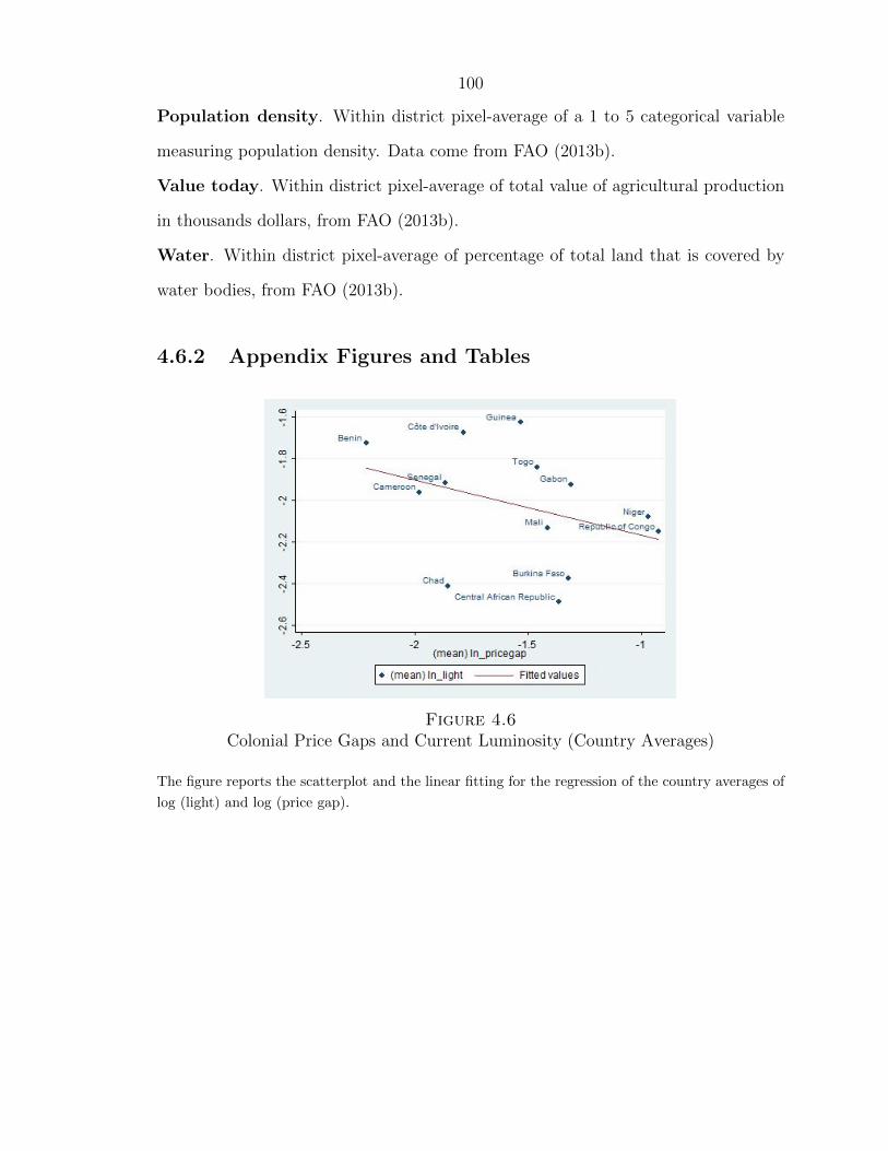
100
Population density. Within district pixel-average of a 1 to 5 categorical variable
measuring population density. Data come from FAO (2013b).
Value today. Within district pixel-average of total value of agricultural production
in thousands dollars, from FAO (2013b).
Water. Within district pixel-average of percentage of total land that is covered by
water bodies, from FAO (2013b).
4.6.2 Appendix Figures and Tables
Figure 4.6Colonial Price Gaps and Current Luminosity (Country Averages)
The figure reports the scatterplot and the linear fitting for the regression of the country averages of
log (light) and log (price gap).

101
(a) Log(Light)
(b) Log(Price Gap)
Figure 4.7Kernel Densities
The top and bottom panel reports the kernel density of log (light) and log (price gap), respectively.

102
(a) Log(Light), Below Top Percentile (b) Log(Light), Above Top Percentile
(c) Log(Light), Below Top Fifth Percentile (d) Log(Light), Above Top Fifth Percentile
Figure 4.8Kernel Densities, Above and Below Top and Fifth Top Percentiles
Panel A and B report the kernel density of the log of average luminosity excluding pixels above and
below the top percentile, respectively. Panel D and C report the kernel densities excluding pixels
above and below the top fifth percentile, respectively.

103
Table4.6
Sum
mar
ySta
tist
ics
Vari
able
Nm
ean
sdp25
p50
p75
min
max
pri
cega
p53
90.
225
0.09
30.
151
0.21
50.
275
0.07
40.
473
log
(pri
cega
p)
539
-1.5
820.
433
-1.8
90-1
.537
-1.2
91-2
.604
-0.7
49p
oten
tial
valu
e19
50s
539
616.
947
670.
223
112.
205
418.
430
844.
163
0.08
833
88.8
70lo
g(p
oten
tial
valu
e19
50s)
539
5.58
91.
675
4.72
06.
037
6.73
8-2
.430
8.12
8pre
-col
onia
lst
ate
centr
aliz
atio
n47
81.
047
0.79
20.
500
1.00
01.
500
0.00
03.
000
Lum
inosi
tyligh
t53
90.
218
0.65
40.
088
0.11
70.
174
0.03
18.
882
log
(lig
ht)
539
-2.0
310.
701
-2.4
30-2
.146
-1.7
49-3
.474
2.18
4%
unlit
539
0.02
30.
062
0.00
00.
002
0.01
70.
000
0.65
1%
rura
l53
90.
948
0.11
50.
954
0.98
40.
995
0.00
11.
000
%urb
an53
90.
029
0.09
90.
001
0.00
40.
016
0.00
00.
999
urb
anligh
t50
511
0.50
628
2.52
49.
794
23.2
4576
.090
1.67
828
94.3
70ru
ral
ligh
t53
90.
122
0.05
40.
085
0.10
80.
150
0.02
90.
429
ln(u
rban
ligh
t)50
53.
390
1.51
62.
282
3.14
64.
332
0.51
87.
971
ln(r
ura
lligh
t)53
9-2
.190
0.41
6-2
.465
-2.2
26-1
.897
-3.5
40-0
.846
Geogra
phy
Contr
ols
fore
st53
929
.200
26.3
585.
122
25.3
0340
.528
0.00
088
.874
wat
er53
90.
681
1.88
80.
000
0.00
00.
259
0.00
016
.478
des
ert
539
1.52
96.
787
0.00
00.
000
0.00
00.
000
63.3
50el
evat
ion
539
350.
970
220.
424
220.
971
327.
237
462.
451
0.00
013
12.0
00cu
ltiv
ated
539
17.9
7216
.195
2.91
514
.803
29.1
960.
017
74.7
12m
alar
ia53
90.
458
0.14
50.
378
0.47
80.
556
0.01
60.
726
Reso
urc
es
Contr
ols
live
stock
539
3.13
11.
476
1.81
03.
294
4.35
70.
246
7.59
1oi
l53
90.
069
0.25
30.
000
0.00
00.
000
0.00
01.
000
dis
tance
top
ort
539
5.15
73.
683
2.08
24.
415
7.84
80.
059
16.8
63va
lue
today
539
343.
784
334.
997
52.4
0625
5.44
955
7.64
40.
013
1539
.752
log
(val
ue
today
)53
94.
971
1.76
13.
959
5.54
36.
324
-4.3
437.
339
pop
ula
tion
den
sity
539
3.41
2.9
193
.000
4.00
04.
000
1.00
05.
000
Ple
ase
see
the
Dat
aA
pp
end
ixfo
rd
etail
edd
efin
itio
ns
an
dso
urc
es.

104
Table 4.7Prices Are Measured at Exit Ports
(1)Price Africa
Price France 0.747∗∗∗
(0.00617)
Landlocked Colony -0.0171(0.0113)
N 39R2 0.951
The table reports OLS estimates of the
relationship between price in Africa,
price in Africa, and whether the coun-
try has a port (landlocked colony
dummy). Please see the Data Ap-
pendix for detailed definitions and
sources. Robust standard errors clus-
tered at the commodity level are re-
ported in parenthesis. *** p<10%,
**p<5%, *p<10%.

105
Table4.8
Rura
lU
nder
dev
elop
men
tor
Low
erU
rban
izat
ion:
Exte
nsi
veM
argi
n(T
opF
ifth
Per
centi
le)
(1)
(2)
(3)
(4)
(5)
(6)
(7)
(8)
%b
elow
top
fift
hp
erce
nti
le%
top
fift
hp
erce
nti
le
Log
(pri
cega
p)
0.11
8**
0.07
72**
*0.
278*
**0.
140*
-0.1
29**
*-0
.086
0***
-0.3
01**
*-0
.173
**(0
.050
9)(0
.025
2)(0
.066
5)(0
.068
1)(0
.041
7)(0
.021
1)(0
.066
1)(0
.064
2)
Cou
ntr
yF
ixed
Eff
ects
Yes
Yes
Yes
Yes
Geo
grap
hy
Con
trol
sY
esY
esY
esY
esR
esou
rces
Con
trol
sY
esY
esY
esY
esL
og(p
oten
tial
valu
e19
50s)
Yes
Yes
Yes
Yes
N53
953
953
953
953
953
953
953
9R
20.
077
0.34
70.
094
0.23
50.
104
0.31
50.
115
0.24
9
Th
eta
ble
rep
orts
OL
Ses
tim
ates
ofth
ere
lati
on
ship
bet
wee
nco
lon
ialp
rice
gap
san
dth
esh
are
ofp
ixel
sw
ith
inea
chd
istr
ict
wit
hze
rolu
min
osi
ty
(col
um
ns
1-4)
,lu
min
osit
yb
elow
the
top
fift
hp
erce
nti
le(c
olu
mn
s5-8
),an
dab
ove
the
top
fift
hp
erce
nti
le(c
olu
mn
s9-1
2).
Geo
gra
phy
contr
ols
incl
ud
ep
erce
nta
geof
land
cove
red
by
fore
st,
des
ert,
an
dw
ate
r,p
erce
nta
ge
of
cult
ivate
dla
nd
,av
erage
elev
atio
n,
an
dm
ala
ria
suit
ab
ilit
yin
dex
;
reso
urc
esco
ntr
ols
incl
ud
eli
vest
ock
,lo
gva
lue
of
curr
ent
agri
cult
ura
lp
rod
uct
ion
,p
op
ula
tion
den
sity
,li
nea
rd
ista
nce
toth
ecl
ose
stp
ort
,an
d
oil
du
mm
y.In
the
spec
ifica
tion
sw
ith
fixed
effec
ts,
theR
2m
easu
res
the
exp
lain
edva
riance
wit
hin
cou
ntr
ies.
Rob
ust
stan
dard
erro
rscl
ust
ered
atth
eco
untr
yle
vel
are
rep
orte
din
par
enth
esis
.***
p<
10%
,**p<
5%
,*p<
10%
.

106
Table4.9
Rura
lU
nder
dev
elop
men
tor
Low
erU
rban
izat
ion:
Inte
nsi
veM
argi
n(T
opF
ifth
Per
centi
le)
(1)
(2)
(3)
(4)
(5)
(6)
(7)
(8)
log
(lig
ht,
top
fift
hp
erce
nti
le)
log
(lig
ht,
bel
owto
pfift
hp
erce
nti
le)
Log
(pri
cega
p)
0.03
590.
116
-0.0
371
-0.1
09-1
.685
**-1
.271
***
-2.9
62**
-1.4
53*
(0.1
79)
(0.1
12)
(0.2
28)
(0.2
06)
(0.6
49)
(0.3
82)
(1.0
11)
(0.7
74)
Cou
ntr
yF
ixed
Eff
ects
Yes
Yes
Yes
Yes
Geo
grap
hy
Con
trol
sY
esY
esY
esY
esR
esou
rces
Con
trol
sY
esY
esY
esY
esL
og(p
oten
tial
valu
e19
50s)
Yes
Yes
Yes
Yes
N53
553
553
553
553
053
053
053
0R
20.
000
0.21
70.
000
0.07
50.
106
0.42
10.
102
0.23
4
Th
eta
ble
rep
orts
OL
Ses
tim
ates
ofth
ere
lati
on
ship
bet
wee
nco
lon
ial
pri
cegap
san
dth
eav
erage
lum
inosi
tyw
ith
inea
chd
istr
ict,
com
pu
ted
amon
gp
ixel
sab
ove
(col
um
ns
1-4
)an
db
elow
the
top
fift
hp
erce
nti
le(c
olu
mn
s5-8
).G
eogra
phy
contr
ols
incl
ud
e
per
centa
geof
lan
dco
ver
edby
fore
st,
des
ert,
an
dw
ate
r,p
erce
nta
ge
of
cult
ivate
dla
nd
,av
erage
elev
atio
n,
an
dm
ala
ria
suit
ab
ilit
y
ind
ex;
reso
urc
esco
ntr
ols
incl
ud
eli
vest
ock
,lo
gva
lue
of
curr
ent
agri
cult
ura
lp
rod
uct
ion
,p
op
ula
tion
den
sity
,li
nea
rd
ista
nce
toth
e
clos
est
por
t,an
doi
ld
um
my.
Inth
esp
ecifi
cati
on
sw
ith
fixed
effec
ts,
theR
2m
easu
res
the
exp
lain
edva
rian
cew
ithin
cou
ntr
ies.
Rob
ust
stan
dar
der
rors
clu
ster
edat
the
cou
ntr
yle
vel
are
rep
ort
edin
pare
nth
esis
.***
p<
10%
,**p<
5%
,*p<
10%
.
107
Chapter 5
Conclusion
In the recent years, a growing body of studies about current African underdevelop-
ment has emphasized the role of extractive institutions established by the colonizers.
However, much more limited efforts have been undertaken to understand the details
of colonial extraction, why extractive institutions were adopted, and how they evolved
over time. In this work, I attempted to “decompress history” more than what has
been done so far in the literature, opening the “black box” of extractive institutions,
analyzing their role during the colonial period, and quantifying colonial extraction.
In doing so, I focused on the relatively under-studied French colonies. I demon-
strated that the colonizers were extremely successful in extracting income from Africans
and that they were able to do so by reducing the prices to agricultural producers
through a combination of trading monopsonies and coercive labor institutions.
Such extractive institutions, however, were not adopted everywhere and the level
of extraction varied greatly across colonies. To explain this finding, I showed that
the choice of institutions was affected more by the kind of commodities that were
produced than by the local conditions of the colonies.
This variation in extraction, together with the persistence of colonial institutions
after independence, can explain the different paths of growth in African countries and
108
regions. My analysis suggests that colonial extraction affected subsequent growth in
particular by reducing development in rural areas to the benefit of a urban elite,
increasing in this way the rural-urban development gap. The different impact on
rural and urban areas can be the reason why colonial extractive institutions persisted
long after independence.
These results call for future research. First, it would be interesting to explore
the post-colonial governments’ incentives to maintain such institutions, despite their
negative effect on economic growth. Are these incentives affected by local factors, such
as the type of political support (urban or rural based) that independent government
received? Or are they shaped by international factors, such as trade relationships
between Africa and the rest of the world? What was then the impact of the trade
liberalizations in the 1980s and 1990s?
Another promising line of research is a comparison with the British colonies. Since
the extent of monopsonies was more limited than in the French colonies, British
Africa stands as a natural counterfactual to study the effects of colonial institutions.
To understand the differences between French and British policies towards African
farmers, it would be particularly interesting to analyze prices to producers in colonies
that were partitioned into a British and a French part after WWI, such as Togo
or Cameroon. Finally, the higher population density of the British colonies allowed
the colonizer to implement different coercive institutions, such as land alienation,
in order to acquire the African labor force. Comparing British and French colonies
would provide the opportunity to disassociate the effects of land coercion and labor
coercion.
109
Bibliography
D. Acemoglu and J. Robinson. Why Nations Fail: The Origins of Power, Prosperity,
and Poverty. Crown Publishing Group, 2012.
D. Acemoglu, S. Johnson, and J. Robinson. The colonial origins of comparative
development: An empirical investigation. American Economic Review, 91:1369–
1401, 2001.
D. Acemoglu, S. Johnson, and J. Robinson. Reversal of fortune: Geography and
institutions in the making of the modern world income distribution. Quarterly
Journal of Economics, 117:1232–1294, 2002.
L. Arias and D. Girod. Indigenous origins of colonial institutions. Working paper,
2011.
G. Austin. The “reversal of fortune” thesis and the compression of history: Per-
spectives from African and comparative economic history. Journal of International
Development, 20:996–1027, 2008.
R. Bates. Markets and States in Tropical Africa: The Political Basis of Agricultural
Policies. University of California Press, 1981.
R. Bates. Essays on the political economy of rural Africa. University of California
Press, 1983.

110
R. Bates and S. Block. Political economy of agricultural trade interventions in Africa.
Agricultural Distortions Working Paper, 87, 2009.
E. J. Berg. The development of a labor force in Sub-Saharan Africa. Economic
Development and Cultural Change, 13(4):394–412, 1965.
D. Berger. Taxes, institutions, and local government: evidence from a natural exper-
iment in colonial Nigeria. Working Paper, 2009.
Cameroun. Statistiques Commerciales. Chambre de Commerce du Cameroun, 1935-
37.
Cameroun. Annuaire statistique du Cameroun, v.1, 1938/45. Service de la statistique
generale, 1947.
D. Cogneau and A. Moradi. Borders that divide: Education and religion in Ghana
and Togo since colonial times. Journal of Economic History, forthcoming, 2014.
C. Coquery-Vidrovitch. Colonialism in Africa, 1870-1970, vol. 1, chapter French
Colonization in Africa to 1920: administration and economic development, pages
165–198. Cambridge University Press, 1969.
C. Coquery-Vidrovitch. Le Congo au temps des grandes compagnies concessionnaires,
1898-1930. Mouton De Gruyter, 1972.
D. Cordell and J. W. Gregory. Labour reservoirs and population: French colonial
strategies in Koudougou, Upper Volta, 1914 to 1939. Journal of African History,
23(2):205–224, 1982.
E. DeDampierre. Coton noir, cafe blanc. Deux cultures du Haut-Oubangui a la veille
de la loi-cadre. Cahiers d’etudes africaines, 1(2):128–147, 1960.
E. Domar. The causes of slavery: a hypothesis. Journal of Economic History, 30:
18–32, 1969.
111
P. Duignan and L. H. Gahan. Colonialism in Africa, 1870-1960. Cambridge Univer-
sity Press, 1975.
S. Engerman and K. Sokoloff. Factor endowments, inequality, and paths of develop-
ment among new world economies. NBER Working Paper 9259, 2002.
P. Englebert. Pre-colonial institutions, post-colonial states, and economic develop-
ment in tropical Africa. Political Research Quarterly, 53:7 36, 2000.
J.D. Fage and R. Olivier. The Cambridge history of Africa. Cambridge University
Press, 1986.
B. Fall. Le travail force en AOF, 1900-1946. KARTHALA Editions, 1993.
FAO. Faostat trade database, 2013a. URL http://faostat.fao.org/.
FAO. Gaez v.3.0 global agro-ecological zones. http://gaez.fao.org/, 2013b.
J. Fenske. Does land abundance explain African institutions? Economic Journal,
123:13631390, 2013.
France. Statistiques coloniales. Commerce. Ministere des Colonies. Office Colonial,
1898-1906.
France. Statistiques du commerce exterieur de la France. Direction generale des
douanes et droits indirects, 1902-1959.
France. Statistiques du commerce de colonies Francaises. Ministere des Colonies.
Office Colonial, 1909-1914.
France. Reinsegnements generaux sur le commerce des colonies Francaises. Docu-
ments statistiques sur les principaux produits exportes. Ministere des Colonies.
Office Colonial, 1920-28.
France. Annuaire Statistique de France. Statistique generale, 1935.
112
France. Statistiques du Commerce Exterieur de l’AEF, 1936-47. Ministere de la
France d’Outremer, 1948.
France. Documents et Statistiques, 1949-1967. Ministere de la France d’ Outremer,
1967.
France-Inflation.com, 2012. URL http://france-inflation.com/.
E. Frankema and M. van Waijenburg. Structural impediments to African growth?
New evidence from real wages in British Africa, 1880-1965. Journal of Economic
History, 72(4):895–926, 2012.
French Equatorial Africa. Annuaire Statistique de l’AEF, vol. 1936-50 and 1951-55.
Service de la statistique generale.
French Equatorial Africa. Bulletin economique de l’Afrique Equatoriale Francaise.
Gouvernement general de l’Afrique Equatoriale Francaise, 1931-36.
French West Africa. Bulletin de la Statistique Generale de l’AOF, 1946-1956. Service
de la statistique generale.
French West Africa. Bulletin mensuel. Agence economique du Gouvernement general
de l’Afrique occidentale francaise, 1930-39.
French West Africa. Annuaire Statistique de l’Afrique Occidentale Francaise. Service
de la statistique generale, 1933-38.
French West Africa. Annuaire Statistique de l’Afrique Occidentale Francaise, 1950-
54. Service de la statistique generale, 1955.
French West Africa. Bulletin statistique et economique mensuel. Service de la statis-
tique generale, 1959-60.

113
F. Gallego and R. Woodberry. Christian missionaries and education in former
colonies: How competition mattered. Journal of African Economies, 19(3):294–
329, 2010.
J.L Gallup and J. Sachs. The economic burden of malaria. American Journal of
Tropical Medicine and Hygiene, 64(1):85–96, 2001.
Patil A.P. Smith D.L. Guerra C.A. Elyazar I.R.F. Johnston G.L. Tatem A.J. Hay S.I.
Gething, P.W. A new world malaria map: Plasmodium falciparum endemicity in
2010. Malaria Journal, 10:378, 2011.
C. Gray and F. Ngolet. Lambarene, okoume and the transformation of labor along
the Middle Ogooue (Gabon), 1870-1945. Journal of African History, 40:87–107,
1999.
J. Herbst. States and Power in Africa: Comparative Lessons in Authority and Control.
Princeton University Press, 2000.
A. G. Hopkins. An economic history of West Africa. Columbia University Press,
1973.
E. Huillery. History matters: The long term impact of colonial public investments
in French West Africa. American Economic Journal - Applied Economics, 1(2):
176–215, 2009.
D. Jacks, K. O’Rourke, and J. Williamson. Commodity price volatility and world
market integration since 1700. Review of Economics and Statistics, 93(3):800–813,
2011.
M. Jerven. The quest for the African dummy: explaining African post-colonial eco-
nomic performance revisited. Journal of International Development, 23(2):288–307,
2011.

114
P. Manning. Francophone Sub-Saharan Africa 1880-1995. Cambridge University
Press, 1998.
N. Maurer and C. Yu. What T. R. took: The economic impact of the Panama canal,
1903-1937. Journal of Economic History, 68(3):686–721, 2008.
S. Michalopoulos. The origins of ethnolinguistic diversity. American Economic Re-
view, 102(4):15081539, 2012.
S. Michalopoulos and E. Papaioannou. The long-run effects of the scramble for Africa.
Working Paper, 2011.
S. Michalopoulos and E Papaioannou. Pre-colonial ethnic institutions and contem-
porary African development. Econometrica, 81:113–152, 2013.
B. Mitchell. Abstract of British Historical Statistics. Cambridge University Press,
1988.
S. Mohammed and J. Williamson. Freight rates and productivity gains in British
tramp shipping 1869-1950. Explorations in Economic History, 41(2):172–203, 2004.
G. P. Murdock. Ethnographic Atlas. University of Pittsburgh Press, Pittsburgh, 1967.
NOAA National Geophysical Data Center. VIIRS DNB Cloud Free Composites.
http : //ngdc.noaa.gov/eog/viirs/, 2013.
N. Nunn. Historical legacies: A model linking Africa’s past to its current underde-
velopment. Journal of Development Economics, 83:157–175, 2007.
N. Nunn. Religious conversion in colonial Africa. American Economic Review Papers
and Proceedings, 100(2):147–152, 2010.
N. Nunn and D. Puga. Ruggedness: The blessing of bad geography in Africa. The
Review of Economics and Statistics, 94(1):20–36, 2012.

115
N. Nunn and L. Wantchekon. The slave trade and the origins of mistrust in Africa.
American Economic Review, 101(7):3221–52., 2011.
L. H. Officer. Exchange rates between the United States dollar and forty-one curren-
cies. MeasuringWorth, URL: http://www.measuringworth.com/exchangeglobal/,
2013.
W. Rodney. How Europe Underdeveloped Africa. Bogle-L’Ouverture Publications,
1972.
J. Suret-Canale. French colonialism in tropical Africa, 1900-1945. Pica Press, 1971.
F. Tadei. Extractive institutions and gains from trade: Evidence from colonial Africa.
Working Paper, California Intitute of Technology, 2013.
B. E. Thomas. Railways and ports in French West Africa. Economic Geography,
33(1):1–15, 1957.
V. Thompson and R. Adloff. French West Africa. Stanford University Press, 1957.
Togo. Bulletin Statistique Mensuel. Service de la statistique generale, 1957.
Togo-Cameroun. Bulletin mensuel d’information. Agence economique des territoires
africains sous mandat, 1933-37.
United States. Historical Statistics of the United States, Colonial Times to 1970.
Bureau of the Census, 1975.