extreme value theory - unc.edurls/s890/evtclass.pdf · extreme value theory richard l. smith...
TRANSCRIPT

EXTREME VALUE THEORY
Richard L. Smith
Department of Statistics and Operations Research
University of North Carolina
Chapel Hill, NC 27599-3260
Notes for STOR 890 Course
Chapel Hill, Spring Semester 2009
1

Here is an example to motivate the subject from the climate
change perspective.
The year 2003 featured one of the hottest summers on record in
southern Europe. Around 30,000 people are estimated to have
died (in many cases, because they failed to receive adequate
treatment for heatstroke).
It’s not possible for a single event like this to say whether it was
“due to climate change”. But we can ask the following question:
What is the probability that such an event would occur under
present-day climate conditions? And what would that probability
have been if there had been no greenhouse-gas-induced global
warming?
A paper by Stott et al. in Nature addressed that question directly.
2

(From a presentation by Myles Allen)
3

4

5

OUTLINE OF PRESENTATION
I. Extreme value theory
• Probability Models• Estimation• Diagnostics
II. Example: North Atlantic Storms
III. Example: European Heatwave
IV. Example: Wang Junxia’s Record
V. Example: Insurance Extremes
VI. Example: Trends in Extreme Rainfall Events
VII. Multivariate Extremes and Max-stable Processes
6

I. EXTREME VALUE THEORY
7
EXTREME VALUE DISTRIBUTIONS
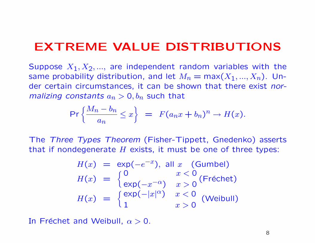
Suppose X1, X2, ..., are independent random variables with thesame probability distribution, and let Mn = max(X1, ..., Xn). Un-der certain circumstances, it can be shown that there exist nor-malizing constants an > 0, bn such that
Pr{Mn − bnan
≤ x}
= F (anx+ bn)n → H(x).
The Three Types Theorem (Fisher-Tippett, Gnedenko) assertsthat if nondegenerate H exists, it must be one of three types:
H(x) = exp(−e−x), all x (Gumbel)
H(x) ={0 x < 0
exp(−x−α) x > 0(Frechet)
H(x) ={
exp(−|x|α) x < 0
1 x > 0(Weibull)
In Frechet and Weibull, α > 0.
8

The three types may be combined into a single generalized ex-
treme value (GEV) distribution:
H(x) = exp
−(
1 + ξx− µψ
)−1/ξ
+
,(y+ = max(y,0))
where µ is a location parameter, ψ > 0 is a scale parameter
and ξ is a shape parameter. ξ → 0 corresponds to the Gumbel
distribution, ξ > 0 to the Frechet distribution with α = 1/ξ, ξ < 0
to the Weibull distribution with α = −1/ξ.
ξ > 0: “long-tailed” case, 1− F (x) ∝ x−1/ξ,
ξ = 0: “exponential tail”
ξ < 0: “short-tailed” case, finite endpoint at µ− ξ/ψ9
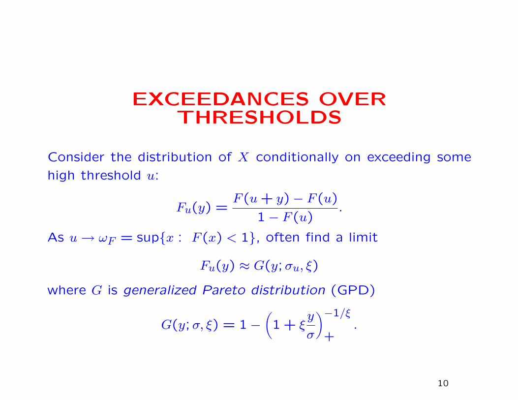
EXCEEDANCES OVERTHRESHOLDS
Consider the distribution of X conditionally on exceeding some
high threshold u:
Fu(y) =F (u+ y)− F (u)
1− F (u).
As u→ ωF = sup{x : F (x) < 1}, often find a limit
Fu(y) ≈ G(y;σu, ξ)
where G is generalized Pareto distribution (GPD)
G(y;σ, ξ) = 1−(
1 + ξy
σ
)−1/ξ
+.
10

The Generalized Pareto Distribution
G(y;σ, ξ) = 1−(
1 + ξy
σ
)−1/ξ
+.
ξ > 0: long-tailed (equivalent to usual Pareto distribution), tail
like x−1/ξ,
ξ = 0: take limit as ξ → 0 to get
G(y;σ,0) = 1− exp(−y
σ
),
i.e. exponential distribution with mean σ,
ξ < 0: finite upper endpoint at −σ/ξ.
11
The Poisson-GPD model combines the GPD for the excesses
over the threshold with a Poisson distribtion for the number of
exceedances. Usually the mean of the Poisson distribution is
taken to be λ per unit time.
12

POINT PROCESS APPROACH
Homogeneous case:
Exceedance y > u at time t has probability
1
ψ
(1 + ξ
y − µψ
)−1/ξ−1
+exp
−(
1 + ξu− µψ
)−1/ξ
+
dydt
13

Illustration of point process model.
14

Inhomogeneous case:
• Time-dependent threshold ut and parameters µt, ψt, ξt
• Exceedance y > ut at time t has probability
1
ψt
(1 + ξt
y − µtψt
)−1/ξt−1
+exp
−(
1 + ξtut − µtψt
)−1/ξt
+
dydt• Estimation by maximum likelihood
15

ESTIMATION
GEV log likelihood:
` = −N logψ −(
1
ξ+ 1
)∑i
log
(1 + ξ
Yi − µψ
)−∑i
(1 + ξ
Yi − µψ
)−1/ξ
provided 1 + ξ(Yi − µ)/ψ > 0 for each i.
Poisson-GPD model:
` = N logλ− λT −N logσ −(
1 +1
ξ
) N∑i=1
log(
1 + ξYiσ
)provided 1 + ξYi/σ > 0 for all i.
The method of maximum likelihood states that we choose the
parameters (µ, ψ, ξ) or (λ, σ, ξ) to maximize `. These can be
calculated numerically on the computer.
16

DIAGNOSTICS
Gumbel plots
QQ plots of residuals
Mean excess plot
Z and W plots
17
Gumbel plots
Used as a diagnostic for Gumbel distribution with annual maxima
data. Order data as Y1:N ≤ ... ≤ YN :N , then plot Yi:N against
reduced value xi:N ,
xi:N = − log(− log pi:N),
pi:N being the i’th plotting position, usually taken to be (i−12)/N .
A straight line is ideal. Curvature may indicate Frechet or Weibull
form. Also look for outliers.
18

Gumbel plots. (a) Annual maxima for River Nidd flow series. (b)
Annual maximum temperatures in Ivigtut, Iceland.
19

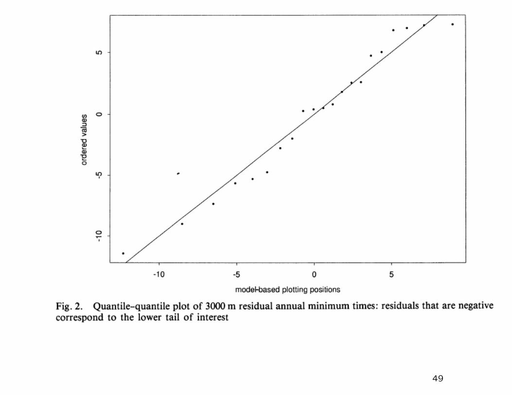
QQ plots of residuals
A second type of probability plot is drawn after fitting the model.
Suppose Y1, ..., YN are IID observations whose common distribu-
tion function is G(y; θ) depending on parameter vector θ. Sup-
pose θ has been estimated by θ, and let G−1(p; θ) denote the
inverse distribution function of G, written as a function of θ. A
QQ (quantile-quantile) plot consists of first ordering the obser-
vations Y1:N ≤ ... ≤ YN :N , and then plotting Yi:N against the
reduced value
xi:N = G−1(pi:N ; θ),
where pi:N may be taken as (i− 12)/N . If the model is a good fit,
the plot should be roughly a straight line of unit slope through
the origin.
Examples...
20

QQ plots for GPD, Nidd data. (a) u = 70. (b) u = 100.
21

Mean excess plot
Idea: for a sequence of values of w, plot the mean excess over
w against w itself. If the GPD is a good fit, the plot should be
approximately a straight line.
In practice, the actual plot is very jagged and therefore its “straight-
ness” is difficult to assess. However, a Monte Carlo technique,
assuming the GPD is valid throughout the range of the plot, can
be used to assess this.
Examples...
22

Mean excess over threshold plots for Nidd data, with Monte Carlo
confidence bands, relative to threshold 70 (a) and 100 (b).
23
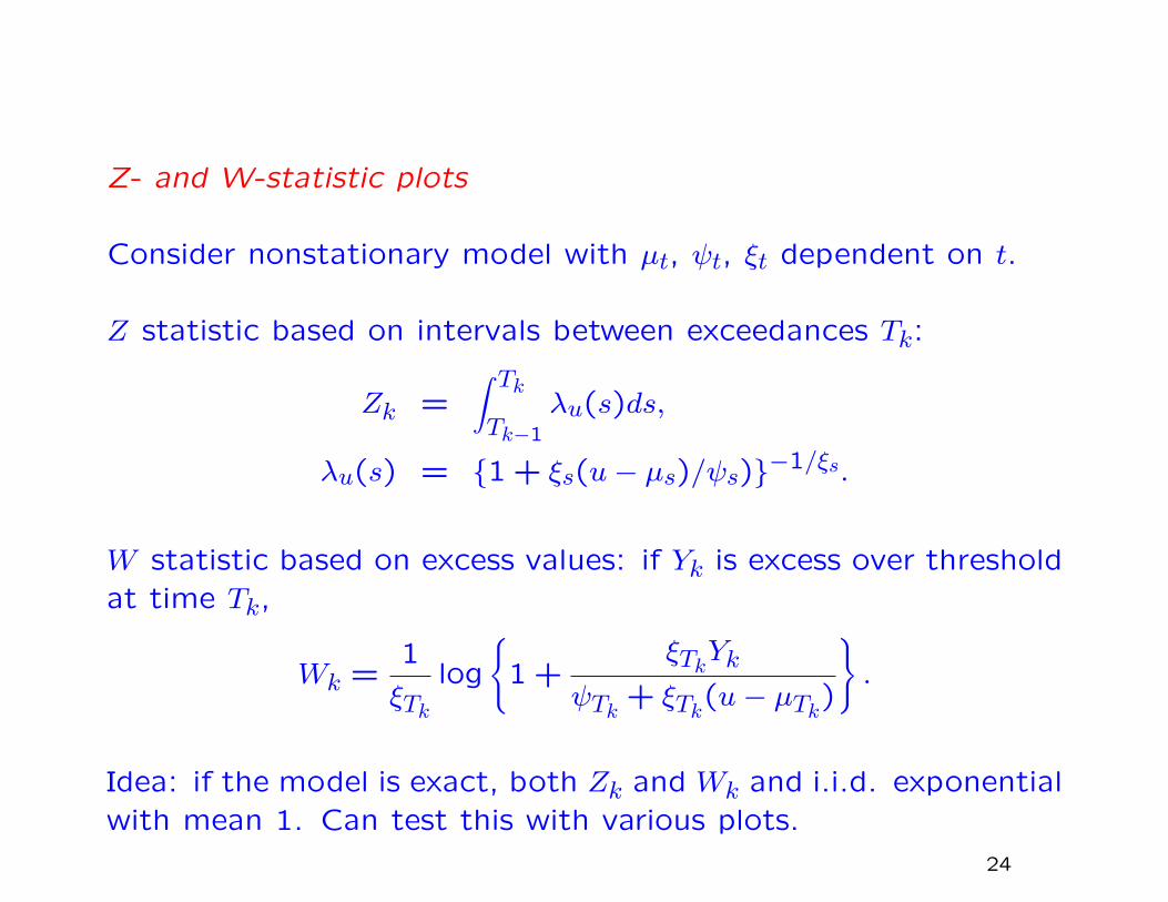
Z- and W-statistic plots
Consider nonstationary model with µt, ψt, ξt dependent on t.
Z statistic based on intervals between exceedances Tk:
Zk =∫ TkTk−1
λu(s)ds,
λu(s) = {1 + ξs(u− µs)/ψs)}−1/ξs.
W statistic based on excess values: if Yk is excess over thresholdat time Tk,
Wk =1
ξTklog
{1 +
ξTkYk
ψTk + ξTk(u− µTk)
}.
Idea: if the model is exact, both Zk and Wk and i.i.d. exponentialwith mean 1. Can test this with various plots.
24

Diagnostic plots based on Z and W statistics for Charlotte wind-
speed data.
25

II. NORTH ATLANTIC CYCLONES
26

Data from HURDAT
Maximum windspeeds in all North Atlantic Cyclones from 1851–
2007
27

1850 1900 1950 2000
4060
8010
012
014
016
0
TROPICAL CYCLONES FOR THE NORTH ATLANTIC
Year
Max
Win
dspe
ed
28

POT MODELS 1900–2007, u=102.5
Model p NLLH NLLH+pGumbel 2 847.8 849.8
GEV 3 843.8 846.8GEV, lin µ 4 834.7 838.7
GEV, quad µ 5 833.4 838.4GEV, cubic µ 6 829.8 835.8
GEV, lin µ, lin logψ 5 828.0 833.0GEV, quad µ, lin logψ 6 826.8 832.8GEV, lin µ, quad logψ 6 827.2 833.2
Fitted model: µ = β0 + β1t, logψ = β2 + β3t, ξ const
β0 β1 β2 β3 ξEstimate 102.5 0.0158 2.284 0.0075 –0.302
S.E. 2.4 0.049 0.476 0.0021 0.066
29
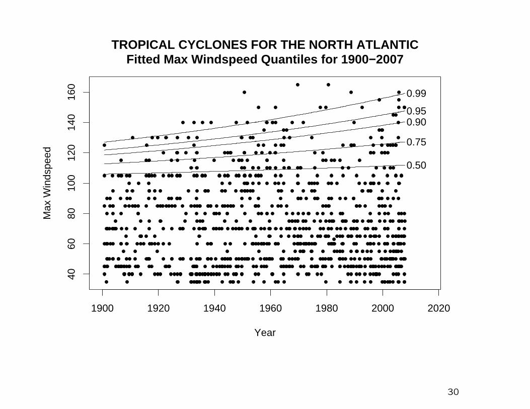
1900 1920 1940 1960 1980 2000 2020
4060
8010
012
014
016
0
TROPICAL CYCLONES FOR THE NORTH ATLANTICFitted Max Windspeed Quantiles for 1900−2007
Year
Max
Win
dspe
ed
0.50
0.75
0.900.95
0.99
30

0 20 40 60 80 100
0
1
2
3
4
5
6
(a)
Time
z va
lue
0 1 2 3 4 5 6
0
1
2
3
4
5
6
(b)
Expected values for z O
bser
ved
valu
es
2 4 6 8 10
−0.15
−0.10
−0.05
0.00
0.05
0.10
0.15
(c)
Lag for z
Cor
rela
tion
0 20 40 60 80 100
0
1
2
3
4
5
6
(d)
Time
w v
alue
0 1 2 3 4 5 6
0
1
2
3
4
5
6
(e)
Expected values for w
Obs
erve
d va
lues
2 4 6 8 10
−0.15
−0.10
−0.05
0.00
0.05
0.10
0.15
(f)
Lag for w
Cor
rela
tion
Diagnostic Plots for Atlantic Cyclones
31

III. EUROPEAN HEATWAVE
32

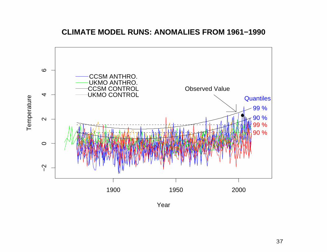
Data:
5 model runs from CCSM 1871–2100, including anthropogenicforcing
2 model runs from UKMO 1861–2000, including anthropogenicforcing
1 model runs from UKMO 2001–2100, including anthropogenicforcing
2 control runs from CCSM, 230+500 years
2 control runs from UKMO, 341+81 years
All model data have been calculated for the grid box from 30–50o
N, 10o W–40o E, annual average temperatures over June–August
Expressed an anomalies from 1961–1990, similar to Stott, Stoneand Allen (2004)
33

1900 1950 2000 2050 2100
−2
02
46
CLIMATE MODEL RUNS: ANOMALIES FROM 1961−1990
Year
Tem
pera
ture
CCSM CONTROL
CCSM ANTHRO.
UKMO CONTROL
UKMO ANTHRO.Observed Value
34

Method:
Fit POT models with various trend terms to the anthropogenic
model runs, 1861–2010
Also fit trend-free model to control runs (µ = 0.176, logψ =
−1.068, ξ = −0.068)
35

POT MODELS 1861–2010, u=1
Model p NLLH NLLH+pGumbel 2 349.6 351.6
GEV 3 348.6 351.6GEV, lin µ 4 315.5 319.5
GEV, quad µ 5 288.1 293.1GEV, cubic µ 6 287.7 293.7GEV, quart µ 7 285.1 292.1
GEV, quad µ, lin logψ 6 287.9 293.9GEV, quad µ, quad logψ 7 287.0 294.9
Fitted model: µ = β0 + β1t+ β2t2, ψ, ξ const
β0 β1 β2 logψ ξEstimate –0.187 –0.030 0.000215 0.047 0.212
S.E. 0.335 0.0054 0.00003 0.212 0.067
36
1900 1950 2000
−2
02
46
CLIMATE MODEL RUNS: ANOMALIES FROM 1961−1990
Year
Tem
pera
ture
CCSM CONTROL
CCSM ANTHRO.
UKMO CONTROL
UKMO ANTHRO.
90 %99 %90 %
99 %
Observed Value
Quantiles
37

200 600 1000
0
1
2
3
4
5
(a)
Time
z va
lue
0 1 2 3 4 5
0
1
2
3
4
5
(b)
Expected values for z O
bser
ved
valu
es
2 4 6 8 10
−0.2
−0.1
0.0
0.1
0.2
(c)
Lag for z
Cor
rela
tion
200 600 1000
0
1
2
3
4
(d)
Time
w v
alue
0 1 2 3 4 5
0
1
2
3
4
(e)
Expected values for w
Obs
erve
d va
lues
2 4 6 8 10
−0.2
−0.1
0.0
0.1
0.2
(f)
Lag for w
Cor
rela
tion
Diagnostic Plots for Temperatures (Control)
38

0 200 400 600 800
0
1
2
3
4
(a)
Time
z va
lue
0 1 2 3 4 5
0
1
2
3
4
(b)
Expected values for z O
bser
ved
valu
es
2 4 6 8 10
−0.2
−0.1
0.0
0.1
0.2
(c)
Lag for z
Cor
rela
tion
0 200 400 600 800
0
1
2
3
4
5
6
(d)
Time
w v
alue
0 1 2 3 4 5
0
1
2
3
4
5
6
(e)
Expected values for w
Obs
erve
d va
lues
2 4 6 8 10
−0.2
−0.1
0.0
0.1
0.2
(f)
Lag for w
Cor
rela
tion
Diagnostic Plots for Temperatures (Anthropogenic)
39

We now estimate the probabilities of crossing various thresholds
in 2003.
Express answer as N=1/(exceedance probability)
Threshold 2.3:
N=3024 (control), N=29.1 (anthropogenic)
Threshold 2.6:
N=14759 (control), N=83.2 (anthropogenic)
40

Comments
1. Differences from Stott-Stone-Allen conclusions arise for two
reasons; different settings of climate models (in particular, I
used “control runs” where they used “natural forcings”); but
also, different climate models. Not clear how much of the
difference is due to inconsistencies between different climate
models. (In particular, use of anomalies from 1961–1990 is
very important, as the different models differ quite a bit in
actual projected temperatures.)
2. A more sophisticated approach would be to use observational
data from 1850–2002 to calibrate the climate models; rather
similar to the approach of Tebaldi et al. (recall opening
classes of this course). This is an open research problem!
41

IV. WANG JUNXIA’S RECORD
References:
Robinson and Tawn (1995), Applied Statistics
Smith (1997), Applied Statistics
42

43

On September 13, 1993, the Chinese athlete Wang Junxia ran
a new world record for the 3000 meter track race in 8 minutes,
6.11 seconds (486.11 sec.).
This improved by 6.08 seconds the record she had run the day
before, which in turn improved by 10.43 seconds on the previ-
ous existing record (502.62 seconds). Both times, she tested
negatively for drugs.
Nevertheless there was widespread suspicion that the record was,
indeed, drug assisted.
Robinson and Tawn compiled a record of the 5 independent best
times each year from 1972–1992, together with Wang’s record.
44

45

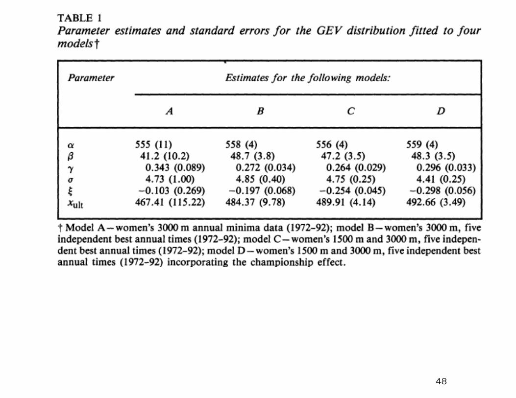
Initial models for the annual minimum:
Gt(x) = 1− exp
−{1−ξ(x− µt)
σ
}−1/ξ
+
,µt = α− β(1− e−γt).
Extended to likelihood based on 5 smallest values per year.
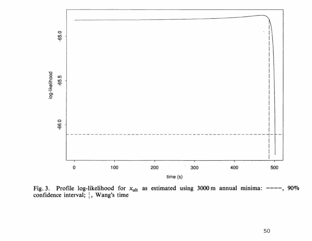
Based on this define
xult =
{α− β + σ
ξ if ξ < 0,
−∞ if ξ ≥ 0.
Profile likelihood for xult: 90% confidence interval based on data
up to 1992 is (0,501.1).
46
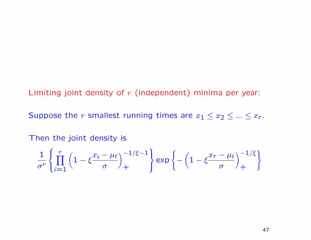
Limiting joint density of r (independent) minima per year:
Suppose the r smallest running times are x1 ≤ x2 ≤ ... ≤ xr.
Then the joint density is
1
σr
r∏
i=1
(1− ξ
xi − µtσ
)−1/ξ−1
+
exp
{−(
1− ξxr − µtσ
)−1/ξ
+
}
47
48
49
50

Smith (1997) suggested instead fitting data form 1980–1992
without trend.
In this model, a 90% confidence interval for xult was (488.2,502.29)
(excluding Wang’s record)
A 95% confidence interval for xult was (481.9,502.43) (including
Wang’s record)
One-sided P-value .039
Still not conclusive
51

52
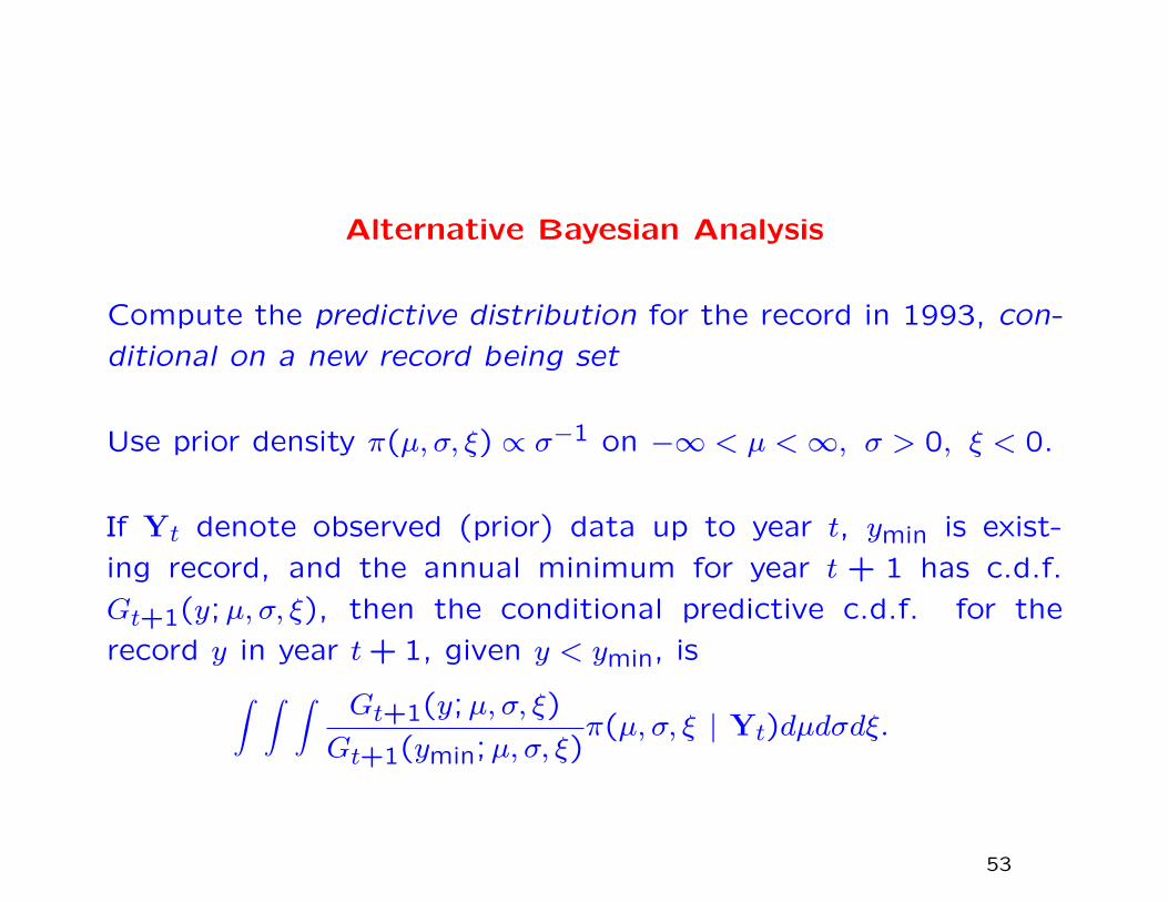
Alternative Bayesian Analysis
Compute the predictive distribution for the record in 1993, con-
ditional on a new record being set
Use prior density π(µ, σ, ξ) ∝ σ−1 on −∞ < µ <∞, σ > 0, ξ < 0.
If Yt denote observed (prior) data up to year t, ymin is exist-
ing record, and the annual minimum for year t + 1 has c.d.f.
Gt+1(y;µ, σ, ξ), then the conditional predictive c.d.f. for the
record y in year t+ 1, given y < ymin, is∫ ∫ ∫ Gt+1(y;µ, σ, ξ)
Gt+1(ymin;µ, σ, ξ)π(µ, σ, ξ | Yt)dµdσdξ.
53
Main Result
Posterior probability of observed record ≤ 486.11 is .00047 (sub-
sequently revised to .0006; see Smith (2003)).
This seems to give much more convincing evidence that Wang’s
record was indeed a very unusual outlier, whether drug-assisted
or not.
54
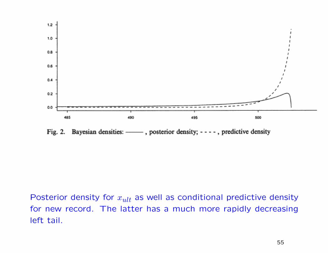
Posterior density for xult as well as conditional predictive density
for new record. The latter has a much more rapidly decreasing
left tail.
55
Take-Home Message
For computing the probability of a specific event, a predictive
distribution may be much more meaningful than a posterior or
likelihood-based interval for some parameter. This leads natu-
rally into Bayesian approaches, because only a Bayesian approach
adequately takes into account both the uncertainty of the un-
known parameters and the randomness of the outcome itself.
Next, we see an example of the same reasoning, applied in the
context of an insurance risk problem.
56

V. INSURANCE EXTREMES(joint work with Dougal Goodman)
57

Oil company data:
(a) Main dataset
(b) cumulative
number of claims
(c) cumulative total claims
(d) mean excess plot
58

Main dataset: 393 insurance claims experienced by a large oil
company, subdivided into 6 classes of claim
Objective to characterize risk to the company from future ex-
treme claims
Initial analysis: fit GPD and point process model to exceedances
over various thresholds.
59

Fitted parameters for GPD model
60

Fitted parameters for point process model
61
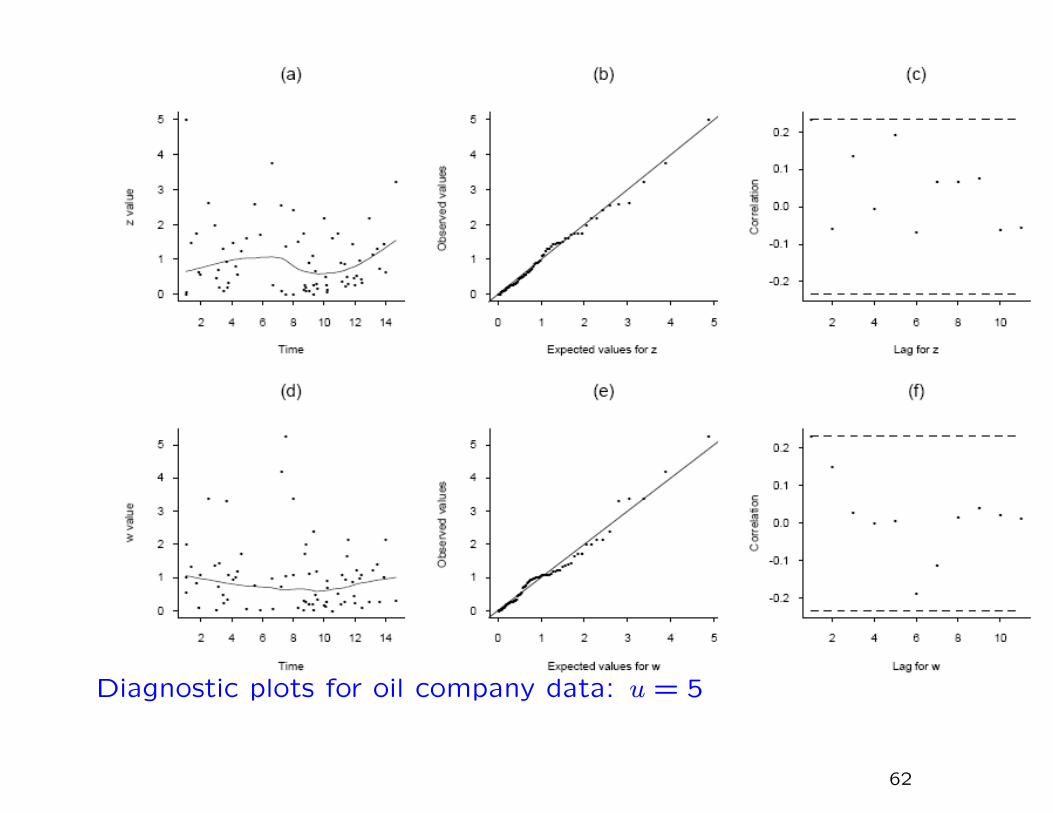
Diagnostic plots for oil company data: u = 5
62

We used a Bayesian analysis to calculate predictive distribution
of claim in a future year (similar to Wang Junxia analysis)
63

Posterior densities for µ and logψ: 4 realizations
64

Posterior densities for ξ and predictive DF: 4 realizations
65

Hierarchical Analysis
Preliminary analyses indicate:
1. When separate GPDs are fitted to each of the 6 types of
claim, there are clear difference among the parameters.
2. The rate of high-threshold crossings does not appear to be
uniform over the years, but peaks around years 10–12.
66

Level I. Parameters mµ, mψ, mξ, s2µ, s
2ψ, s
2ξ are generated from
a prior distribution.
Level II. Conditional on the parameters in Level I, parameters
µ1, ..., µJ (where J is the number of types) are independently
drawn from N(mµ, s2µ), the normal distribution with mean mµ,
variance s2µ. Similarly, logψ1, ..., logψJ are drawn independently
from N(mψ, s2ψ), ξ1, ..., ξJ are drawn independently from N(mξ, s
2ξ ).
Level III. Conditional on Level II, for each j ∈ {1, ..., J}, the
point process of exceedances of type j is a realisation from the
homogeneous point process model with parameters µj, ψj, ξj.
67

This model may be further extended to include a year effect.
Suppose the extreme value parameters for type j in year k are
not µj, ψj, ξj but µj + δk, ψj, ξj. In other words, we allow for a
time trend in the µj parameter, but not in ψj and ξj. We fix
δ1 = 0 to ensure identifiability, and let {δk, k > 1} follow an
AR(1) process:
δk = ρδk−1 + ηk, ηk ∼ N(0, s2η)
with a vague prior on (ρ, s2η).
Run hierarchical model by MCMC.
68
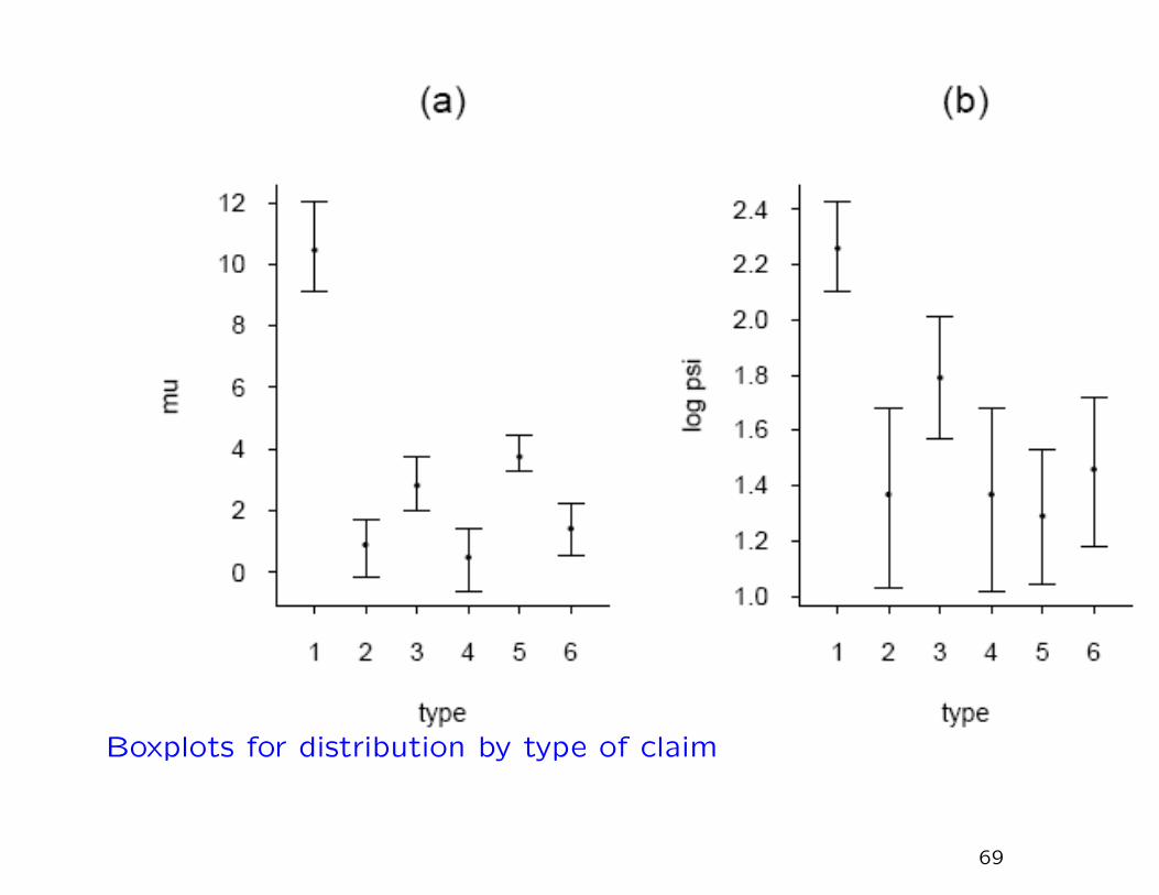
Boxplots for distribution by type of claim
69

Boxplots for distribution by type of claim and year
70

Finally, we collect output from hierarchical model to obtain pre-
dictive distribution of future loss in four cases:
A: All data combined into one sample, no identification of out-
liers, separate type or separate years
B: Identify separate types but not separate years
C: Identify separate types and separate years
D: As C, but omit the two largest observations which may be
outliers
71

4 posterior predictive DFs
72
Take-Home Message
As in the running records example, the Bayesian analysis includ-
ing a posterior distribution seems the best way to express our
uncertainty about future losses.
However, there is an additional benefit in using a hierarchical
model. In this case, fitting separate distributions to each cate-
gory of loss results in less extreme predictions of future losses.
This is possibly because the individual categories have less vari-
ability than if we combine all the claims into a single sample
without regard for category of loss.
73

VI. TREND IN PRECIPITATIONEXTREMES
(joint work with Amy Grady and Gabi Hegerl)
During the past decade, there has been extensive research byclimatologists documenting increases in the levels of extremeprecipitation, but in observational and model-generated data.
With a few exceptions (papers by Katz, Zwiers and co-authors)this literature have not made use of the extreme value distribu-tions and related constructs
There are however a few papers by statisticians that have ex-plored the possibility of using more advanced extreme valuemethods (e.g. Cooley, Naveau and Nychka, JASA 2007; Sangand Gelfand, Environmental and Ecological Statistics, 2008)
This discussion uses extreme value methodology to look fortrends
74
CURRENT METHODOLOGY(see e.g. Groisman et al. 2005)
Most common method is based on counting exceedances over ahigh threshold (e.g. 99.7% threshold)
• Express exceedance counts as anomalies from 30-year meanat each station
• Average over regions using “geometric weighting rule”: firstaverage within 1o grid boxes, then average grid boxes withinregion
• Calculate standard error of this procedure using exponen-tial spatial covariances with nugget (range of 30–500 km,nugget-sill ratio of 0–0.7).
• Increasing trends found in many parts of the world, nearlyalways stronger than trends in precipitation means, but spa-tially and temporally heterogeneous. Strongest increase inUS extreme precipitations is post-1970, about 7% overall
75

DATA SOURCES
• NCDC Rain Gauge Data
– Daily precipitation from 5873 stations
– Select 1970–1999 as period of study
– 90% data coverage provision — 4939 stations meet that
• NCAR-CCSM climate model runs
– 20 × 41 grid cells of side 1.4o
– 1970–1999 and 2070–2099 (A2 scenario)
• PRISM data
– 1405 × 621 grid, side 4km
– Elevations
– Mean annual precipitation 1970–1997
76
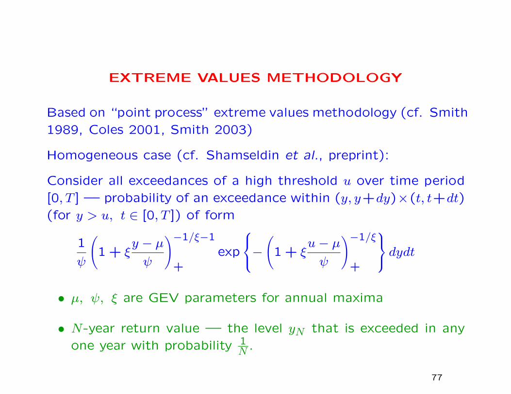
EXTREME VALUES METHODOLOGY
Based on “point process” extreme values methodology (cf. Smith
1989, Coles 2001, Smith 2003)
Homogeneous case (cf. Shamseldin et al., preprint):
Consider all exceedances of a high threshold u over time period
[0, T ] — probability of an exceedance within (y, y+dy)×(t, t+dt)
(for y > u, t ∈ [0, T ]) of form
1
ψ
(1 + ξ
y − µψ
)−1/ξ−1
+exp
−(
1 + ξu− µψ
)−1/ξ
+
dydt• µ, ψ, ξ are GEV parameters for annual maxima
• N-year return value — the level yN that is exceeded in any
one year with probability 1N .
77

Inhomogeneous case:
• Time-dependent threshold ut and parameters µt, ψt, ξt
• Exceedance y > ut at time t has probability
1
ψt
(1 + ξt
y − µtψt
)−1/ξt−1
+exp
−(
1 + ξtut − µtψt
)−1/ξt
+
dydt• Estimation by maximum likelihood
78

Seasonal models without trends
General structure:
µt = θ1,1 +K1∑k=1
(θ1,2k cos
2πkt
365.25+ θ1,2k+1 sin
2πkt
365.25
),
logψt = θ2,1 +K2∑k=1
(θ2,2k cos
2πkt
365.25+ θ2,2k+1 sin
2πkt
365.25
),
ξt = θ3,1 +K3∑k=1
(θ3,2k cos
2πkt
365.25+ θ3,2k+1 sin
2πkt
365.25
).
Call this the (K1,K2,K3) model.
Note: This is all for one station. The θ parameters will differ ateach station.
79

Model selection
Use a sequence of likelihood ratio tests
• For each (K1,K2,K3), construct LRT against some (K′1,K′2,K
′3),
K′1 ≥ K1,K′2 ≥ K2,K
′3 ≥ K3 (not all equal) using standard χ2
distribution theory
• Look at proportion of rejected tests over all stations. If too
high, set Kj = K′j (j = 1,2,3) and repeat procedure
• By trial and error, we select K1 = 4,K2 = 2,K3 = 1 (17
model parameters for each station)
80

Models with trend
Add to the above:
• Overall linear trend θj,2K+2t added to any of µt (j = 1),logψt (j = 1), ξt (j = 1). Define K∗j to be 1 if this term isincluded, o.w. 0.
• Interaction terms of form
t cos2πkt
365.25, t sin
2πkt
365.25, k = 1, ...,K∗∗j .
Typical model denoted
(K1,K2,K3)× (K∗1,K∗2,K
∗3)× (K∗∗1 ,K∗∗2 ,K∗∗3 )
Eventually use (4,2,1)×(1,1,0)×(2,2,0) model (27 parametersfor each station)
81
Details
• Selection of time-varying threshold — based on the 95th
percentile of a 7-day window around the date of interest
• Declustering by r-runs method (Smith and Weissman 1994)
— use r = 1 for main model runs
• Computation via sampling the likelihood: evaluate contribu-
tions to likelihood for all observations above threshold, but
sample only 5% or 10% of those below, then renormalize to
provide accurate approximation to full likelihood
82

Details (continued)
• Covariances of parameters at different sites:
θs is MLE at site s, solves ∇`s(θs) = 0
For two sites s, s′,
Cov(θs, θs′
)≈(∇2`s(θs)
)−1Cov (∇`s(θs),∇`s′(θs′))
(∇2`s′(θs′)
)−1
Estimate covariances on RHS empirically, using a subset of
days (same subset for all stations)
Also employed when s = s′.
Open question: Should we “regularize” this covariance ma-
trix?
83

Details (continued)
• Calculating the N-year return value
For one year (t = 1, ..., T ), find yθ,N numerically to solve
T∑1
(1 + ξt
yθ,N − µtψt
)−1/ξt= − log
(1−
1
N
).
– Also calculate∂yθ,N∂θj
by numerical implementation of in-verse function formula
– Covariances between return level estimates at differentsites by
Cov{yθs,N , yθs′,N
}≈
(dyθs,N
dθs
)TCov
(θs, θs′
)dyθs′,Ndθs′
.– Also apply to ratios of return level estimates, such as
25− year return level at s in 1999
25− year return level at s in 1970
84

SPATIAL SMOOTHING
Let Zs be field of interest, indexed by s (typically the logarithmof the 25-year RV at site s, or a log of ratio of RVs. Taking logsimproves fit of spatial model, to follow.)
Don’t observe Zs — estimate Zs. Assume
Z | Z ∼ N [Z,W ]
Z ∼ N [Xβ, V (φ)]
Z ∼ N [Xβ, V (φ) +W ].
for known W ; X are covariates, β are unknown regression pa-rameters and φ are parameters of spatial covariance matrix V .
• φ by REML
• β given φ by GLS
• Predict Z at observed and unobserved sites by kriging
85

Details
• Covariates
– Always include intercept
– Linear and quadratic terms in elevation and log of mean
annual precipitation
– Contrast “climate space” approach of Cooley et al. (2007)
86

Details (continued)
• Spatial covariances
– Matern
– Exponential with nugget
– Intrinsically stationary model
Var(Zs − Zs′) = φ1dφ2s,s′ + φ3
– Matern with nugget
The last-named contains all the previous three as limiting
cases and appears to be the best overall, though is often
slow to converge (e.g. sometime the range parameter tends
to∞, which is almost equivalent to the intrinsically stationary
model)
87

Details (continued)
• Spatial heterogeneity
Divide US into 19 overlapping regions, most 10o × 10o
– Kriging within each region
– Linear smoothing across region boundaries
– Same for MSPEs
– Also calculate regional averages, including MSPE
88

Continental USA divided into 19 regions
89
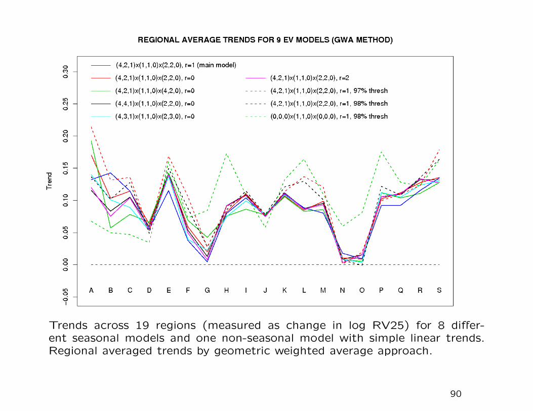
Trends across 19 regions (measured as change in log RV25) for 8 differ-ent seasonal models and one non-seasonal model with simple linear trends.Regional averaged trends by geometric weighted average approach.
90

Summary of models shown on previous slide:
1: Preferred covariates model (r = 0 for declustering, uses 95%
threshold calculated from 7-day window)
2–4: Three variants where we add covariates to µt and/or logψt
5: Replace r = 0 by r = 1 (subsequent results are based on this
model)
6: Replace r = 0 by r = 2
7: 97% threshold calculated from 14-day window
8: 98% threshold calculated from 28-day window
91
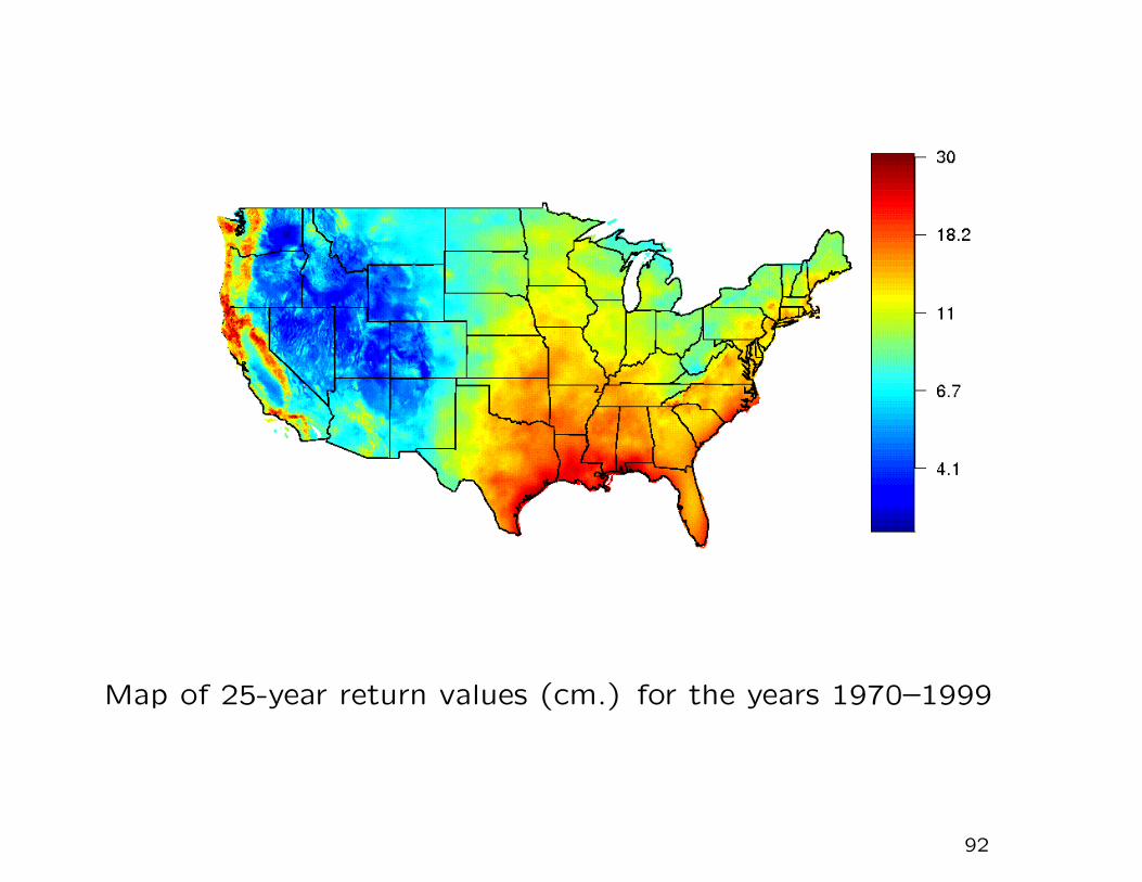
Map of 25-year return values (cm.) for the years 1970–1999
92

Root mean square prediction errors for map of 25-year return
values for 1970–1999
93

Ratios of return values in 1999 to those in 1970
94

Root mean square prediction errors for map of ratios of 25-year
return values in 1999 to those in 1970
95
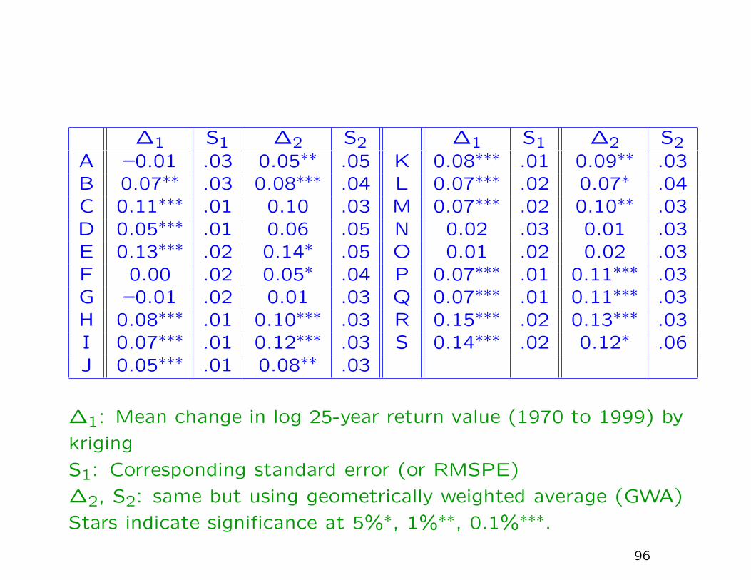
∆1 S1 ∆2 S2 ∆1 S1 ∆2 S2A –0.01 .03 0.05∗∗ .05 K 0.08∗∗∗ .01 0.09∗∗ .03B 0.07∗∗ .03 0.08∗∗∗ .04 L 0.07∗∗∗ .02 0.07∗ .04C 0.11∗∗∗ .01 0.10 .03 M 0.07∗∗∗ .02 0.10∗∗ .03D 0.05∗∗∗ .01 0.06 .05 N 0.02 .03 0.01 .03E 0.13∗∗∗ .02 0.14∗ .05 O 0.01 .02 0.02 .03F 0.00 .02 0.05∗ .04 P 0.07∗∗∗ .01 0.11∗∗∗ .03G –0.01 .02 0.01 .03 Q 0.07∗∗∗ .01 0.11∗∗∗ .03H 0.08∗∗∗ .01 0.10∗∗∗ .03 R 0.15∗∗∗ .02 0.13∗∗∗ .03I 0.07∗∗∗ .01 0.12∗∗∗ .03 S 0.14∗∗∗ .02 0.12∗ .06J 0.05∗∗∗ .01 0.08∗∗ .03
∆1: Mean change in log 25-year return value (1970 to 1999) by
kriging
S1: Corresponding standard error (or RMSPE)
∆2, S2: same but using geometrically weighted average (GWA)
Stars indicate significance at 5%∗, 1%∗∗, 0.1%∗∗∗.
96
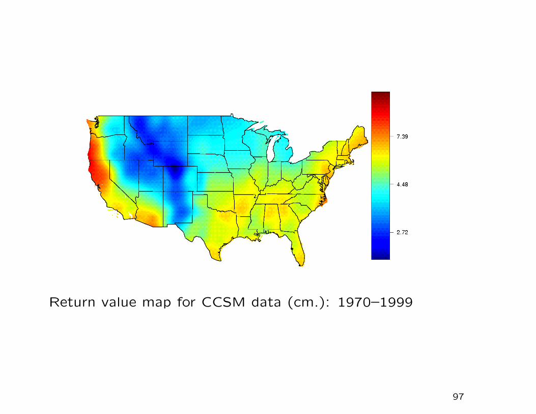
Return value map for CCSM data (cm.): 1970–1999
97

Return value map for CCSM data (cm.): 2070–2099
98

Estimated ratios of 25-year return values for 2070–2099 to those
of 1970–1999, based on CCSM data, A2 scenario
99

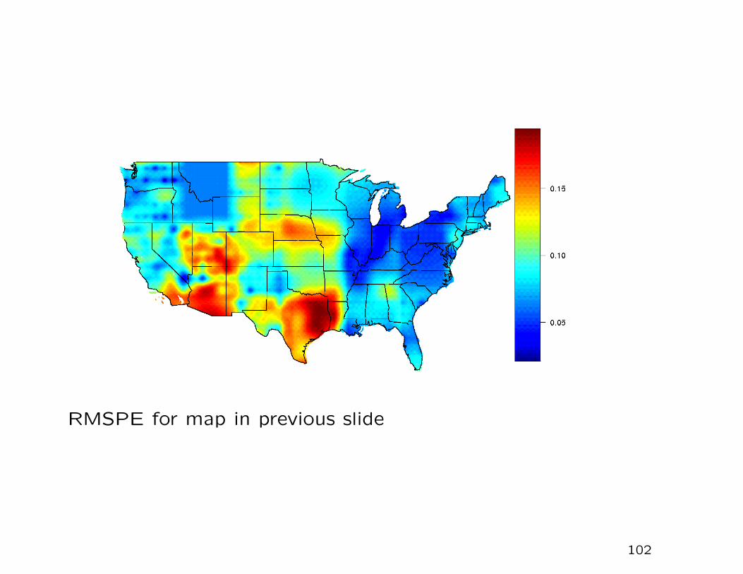
RMSPE for map in previous slide
100

Extreme value model with trend: ratio of 25-year return value in
1999 to 25-year return value in 1970, based on CCSM data
101
RMSPE for map in previous slide
102

∆3 S3 ∆4 S4 ∆3 S3 ∆4 S4A 0.16∗∗ .07 0.24∗∗ .10 K –0.08∗∗∗ .02 –0.11∗ .05B 0.14∗∗∗ .04 0.12∗∗∗ .06 L –0.04 .04 –0.03 .06C 0.02 .05 –0.14 .11 M 0.01 .03 0.00 .08D –0.06 .04 –0.15 .10 N 0.06∗∗ .02 0.05 .06E –0.07∗ .03 –0.09 .08 O –0.03 .04 –0.06 .07F –0.07∗ .04 –0.03 .05 P –0.01 .04 –0.07 .07G 0.03 .03 0.08∗ .04 Q –0.04 .04 –0.03 .07H 0.11∗∗∗ .03 0.08 .06 R –0.17∗∗∗ .03 –0.06 .08I –0.02 .04 –0.05 .07 S 0.00 .04 0.02 .05J –0.15∗∗∗ .03 –0.16∗∗ .06
∆3: Mean change in log 25-year return value (1970 to 1999) for
CCSM, by kriging
SE3: Corresponding standard error (or RMSPE)
∆4, SE4: Results using GWA
Stars indicate significance at 5%∗, 1%∗∗, 0.1%∗∗∗.
103

RETURN VALUE MAPS FOR INDIVIDUAL DECADES
104

Map of 25-year return values (cm.) for the years 1950–1959
105

Map of 25-year return values (cm.) for the years 1960–1969
106

Map of 25-year return values (cm.) for the years 1970–1979
107

Map of 25-year return values (cm.) for the years 1980–1989
108

Map of 25-year return values (cm.) for the years 1990–1999
109

Estimated ratios of 25-year return values for 1990s compared
with average at each location over 1950–1989
110

Regional changes in log RV25 for each decade compared with
1950s
111
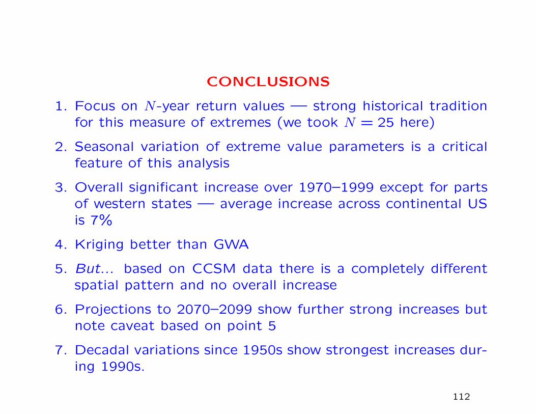
CONCLUSIONS
1. Focus on N-year return values — strong historical traditionfor this measure of extremes (we took N = 25 here)
2. Seasonal variation of extreme value parameters is a criticalfeature of this analysis
3. Overall significant increase over 1970–1999 except for partsof western states — average increase across continental USis 7%
4. Kriging better than GWA
5. But... based on CCSM data there is a completely differentspatial pattern and no overall increase
6. Projections to 2070–2099 show further strong increases butnote caveat based on point 5
7. Decadal variations since 1950s show strongest increases dur-ing 1990s.
112

VII. MULTIVARIATE EXTREMESAND MAX-STABLE PROCESSES
VII.1 Limit theory for multivariate sample maxima
VII.2 Alternative formulations of multivariate extreme value the-
ory
VII.3 Max-stable processes
113

Multivariate extreme value theory applies when we are interested
in the joint distribution of extremes from several random vari-
ables.
Examples:
• Winds and waves on an offshore structure
• Meteorological variables, e.g. temperature and precipitation
• Air pollution variables, e.g. ozone and sulfur dioxide
• Finance, e.g. price changes in several stocks or indices
• Spatial extremes, e.g. joint distributions of extreme precipi-
tation at several locations
114
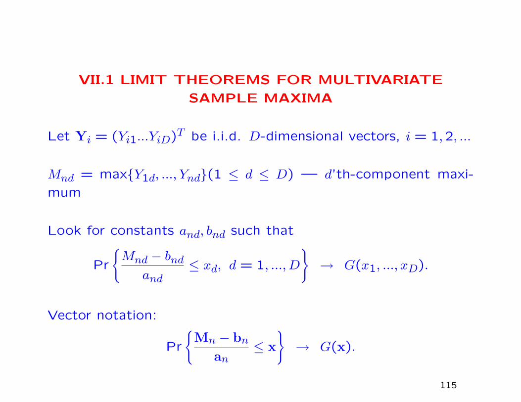
VII.1 LIMIT THEOREMS FOR MULTIVARIATE
SAMPLE MAXIMA
Let Yi = (Yi1...YiD)T be i.i.d. D-dimensional vectors, i = 1,2, ...
Mnd = max{Y1d, ..., Ynd}(1 ≤ d ≤ D) — d’th-component maxi-
mum
Look for constants and, bnd such that
Pr
{Mnd − bnd
and≤ xd, d = 1, ..., D
}→ G(x1, ..., xD).
Vector notation:
Pr
{Mn − bn
an≤ x
}→ G(x).
115

Two general points:
1. If G is a multivariate extreme value distribution, then each
of its marginal distributions must be one of the univariate
extreme value distributions, and therefore can be represented
in GEV form
2. The form of the limiting distribution is invariant under mono-
tonic transformation of each component. Therefore, without
loss of generality we can transform each marginal distribu-
tion into a specified form. For most of our applications, it is
convenient to assume the Frechet form:
Pr{Xd ≤ x} = exp(−x−α), x > 0, d = 1, ..., D.
Here α > 0. The case α = 1 is called unit Frechet.
116

Representations of Limit Distributions
Any MEVD with unit Frechet margins may be written as
G(x) = exp {−V (x)} , (1)
V (x) =∫SD
maxd=1,...,D
(wj
xj
)dH(w), (2)
where SD = {(x1, ..., xD) : x1 ≥ 0, ..., xD ≥ 0, x1 + ... + xD = 1}and H is a measure on SD.
The function V (x) is called the exponent measure and formula(2) is the Pickands representation. If we fix d′ ∈ {1, ..., D} with0 < xd′ <∞, and define xd = +∞ for d 6= d′, then
V (x) =∫SD
maxd=1,...,D
(wdxd
)dH(w) =
1
xd′
∫SD
wd′dH(w)
so to ensure correct marginal distributions we must have∫SD
wddH(w) = 1, d = 1, ..., D. (3)
117

Note that
kV (x) = V
(x
k
)(which is in fact another characterization of V ) so
Gk(x) = exp(−kV (x))
= exp(−V
(x
k
))= G
(x
k
).
Hence G is max-stable. In particular, if X1, ...,Xk are i.i.d. from
G, then max{X1, ...,Xk} (vector of componentwise maxima) has
the same distribution as kX1.
118

The Pickands Dependence Function
In the two-dimensional case (with unit Frechet margins) there is
an alternative representation due to Pickands:
Pr{X1 ≤ x1, X2 ≤ x2} = exp
{−(
1
x1+
1
x2
)A
(x1
x1 + x2
)}where A is a convex function on [0,1] such that A(0) = A(1) =
1, 12 ≤ A
(12
)≤ 1.
The value of A(
12
)is often taken as a measure of the strength of
dependence: A(
12
)= 1
2 is “perfect dependence” while A(
12
)= 1
is independence.
119

VII.1.a EXAMPLES
120

Logistic (Gumbel and Goldstein, 1964)
V (x) =
D∑d=1
x−rd
1/r
, r ≥ 1.
Check:
1. V (x/k) = kV (x)
2. V ((+∞,+∞, ..., xd, ...,+∞,+∞) = x−1d
3. e−V (x) is a valid c.d.f.
Limiting cases:
• r = 1: independent components
• r → ∞: the limiting case when Xi1 = Xi2 = ... = XiD withprobability 1.
121

Asymmetric logistic (Tawn 1990)
V (x) =∑c∈C
∑i∈c
(θi,c
xi
)rc1/rc
,
where C is the class of non-empty subsets of {1, ..., D}, rc ≥1, θi,c = 0 if i /∈ c, θi,c ≥ 0,
∑c∈C θi,c = 1 for each i.
Negative logistic (Joe 1990)
V (x) =∑ 1
xj+
∑c∈C: |c|≥2
(−1)|c|∑i∈c
(θi,c
xi
)rc1/rc
,
rc ≤ 0, θi,c = 0 if i /∈ c, θi,c ≥ 0,∑c∈C(−1)|c|θi,c ≤ 1 for each i.
122
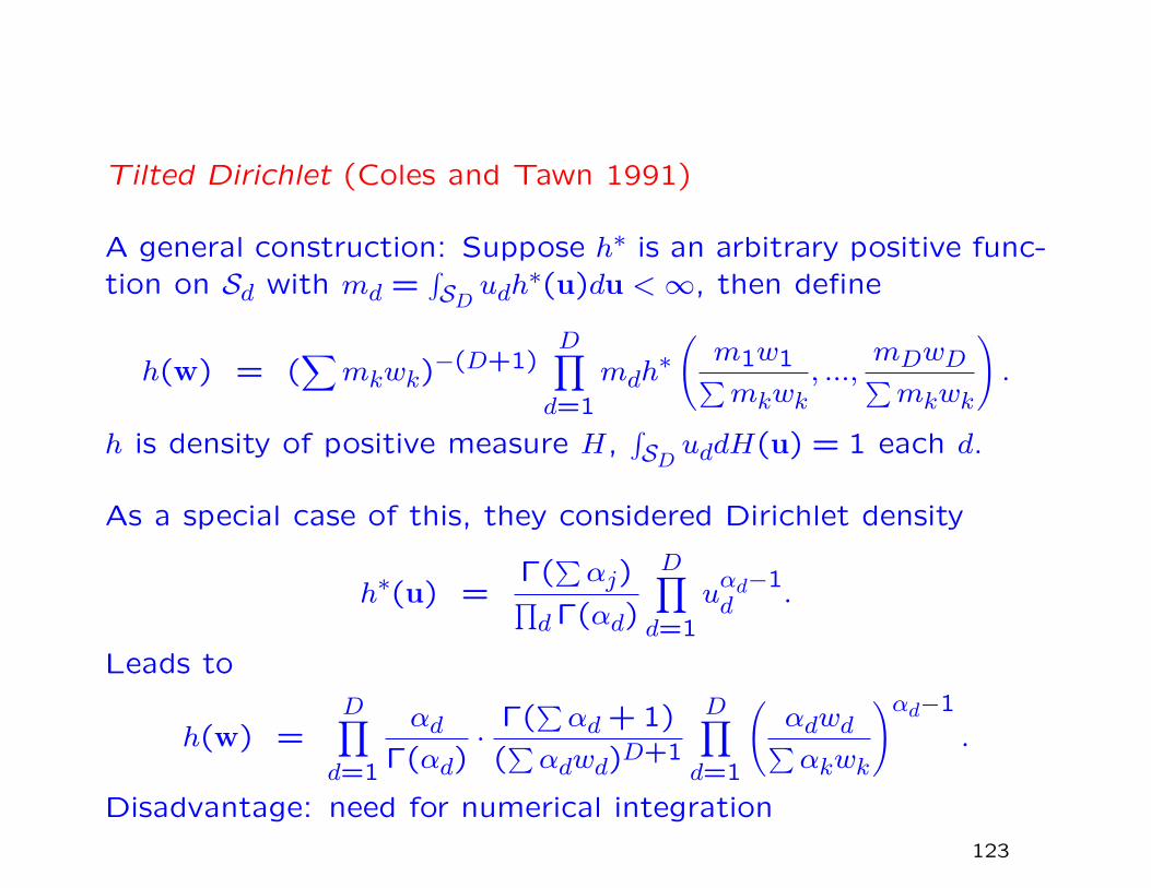
Tilted Dirichlet (Coles and Tawn 1991)
A general construction: Suppose h∗ is an arbitrary positive func-tion on Sd with md =
∫SD udh
∗(u)du <∞, then define
h(w) = (∑
mkwk)−(D+1)D∏d=1
mdh∗(m1w1∑mkwk
, ...,mDwD∑mkwk
).
h is density of positive measure H,∫SD uddH(u) = 1 each d.
As a special case of this, they considered Dirichlet density
h∗(u) =Γ(∑αj)∏
dΓ(αd)
D∏d=1
uαd−1d .
Leads to
h(w) =D∏d=1
αdΓ(αd)
·Γ(∑αd + 1)
(∑αdwd)D+1
D∏d=1
(αdwd∑αkwk
)αd−1
.
Disadvantage: need for numerical integration
123

VII.1.b ESTIMATION
• Parametric
• Non/semi-parametric
Both approaches have problems, e.g. nonregular behavior of
MLE even in finite-parameter problems; curse of dimensionality
if D large.
Typically proceed by transforming margins to unit Frechet first,
though there are advantages in joint estimation of marginal dis-
tributions and dependence structure (Shi 1995)
124

VII.2 ALTERNATIVE FORMULATIONS OF
MULTIVARIATE EXTREMES
125

• Ledford-Tawn-Ramos approach
• Heffernan-Tawn approach
126
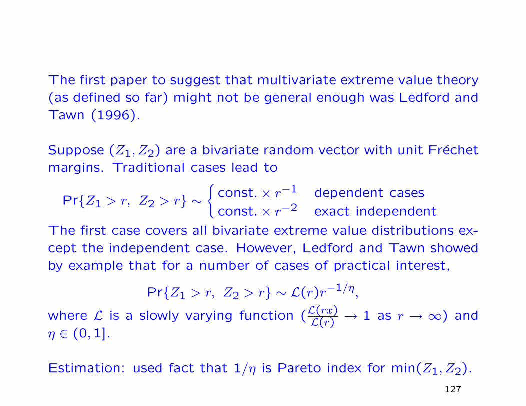
The first paper to suggest that multivariate extreme value theory(as defined so far) might not be general enough was Ledford andTawn (1996).
Suppose (Z1, Z2) are a bivariate random vector with unit Frechetmargins. Traditional cases lead to
Pr{Z1 > r, Z2 > r} ∼{
const.× r−1 dependent cases
const.× r−2 exact independent
The first case covers all bivariate extreme value distributions ex-cept the independent case. However, Ledford and Tawn showedby example that for a number of cases of practical interest,
Pr{Z1 > r, Z2 > r} ∼ L(r)r−1/η,
where L is a slowly varying function (L(rx)L(r) → 1 as r → ∞) and
η ∈ (0,1].
Estimation: used fact that 1/η is Pareto index for min(Z1, Z2).
127
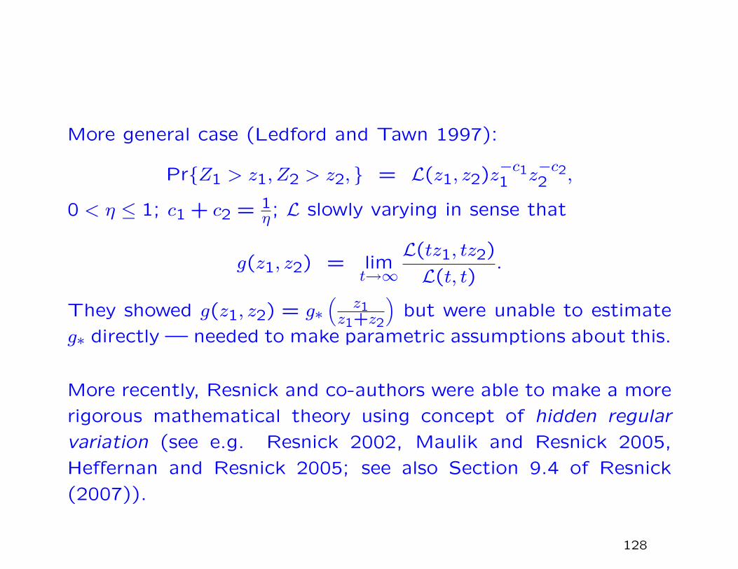
More general case (Ledford and Tawn 1997):
Pr{Z1 > z1, Z2 > z2, } = L(z1, z2)z−c11 z−c22 ,
0 < η ≤ 1; c1 + c2 = 1η ; L slowly varying in sense that
g(z1, z2) = limt→∞
L(tz1, tz2)
L(t, t).
They showed g(z1, z2) = g∗(
z1z1+z2
)but were unable to estimate
g∗ directly — needed to make parametric assumptions about this.
More recently, Resnick and co-authors were able to make a more
rigorous mathematical theory using concept of hidden regular
variation (see e.g. Resnick 2002, Maulik and Resnick 2005,
Heffernan and Resnick 2005; see also Section 9.4 of Resnick
(2007)).
128

Ramos-Ledford (2009, 2008) approach:
Pr{Z1 > z1, Z2 > z2, } = L(z1, z2)(z1z2)−1/(2η),
limu→∞
L(ux1, ux2)
L(u, u)= g(x1, x2)
= g∗
(x1
x1 + x2
)
Limiting joint survivor function
Pr{X1 > x1, X2 > x2} =∫ 1
0η
{min
(w
x1,1− wx2
)}1/η
dH∗η(w),
1 = η∫ 1
0{min (w,1− w)}1/η dH∗η(w).
129

Multivariate generalization to D > 2:
Pr{X1 > x1, ..., XD > xD} =∫SD
η
{min
1≤d≤D
(wdxd
)}1/η
dH∗η(w),
1 =∫SD
η
{min
1≤d≤Dwj
}1/η
dH∗η(w).
Open problems:
• How to find sufficiently rich classes of H∗η(w) to derive para-metric families suitable for real data
• How to do the subsequent estimation
130

The Heffernan-Tawn approach
Reference:
A conditional approach for multivariate extreme values, by Janet
Heffernan and Jonathan Tawn, J.R. Statist. Soc. B 66, 497–
546 (with discussion)
131

A set C ∈ Rd is an “extreme set” if
• we can partition C = ∪di=1Ci where
Ci = C ∩{x ∈ Rd : FXi(xi) > FXj(xj)
}for all i 6= j
(Ci is the set on which Xi is “most extreme” among X1, ..., Xd,extremeness being measured by marginal tail probabilities)
• The set Ci satisfies the following property: there exists a vXisuch that
X ∈ Ci if and only if X ∈ Ci and Xi > vXi.
(or: if X = (X1, ..., Xd) ∈ Ci then so is any other X for whichXi is more extreme)
The objective of the paper is to propose a general methodologyfor estimating probabilities of extreme sets.
132

Marginal distributions
• Standard “GPD” model fit: define a threshold uXi and as-sume
Pr{Xi > uXi + x | Xi > uXi} =
(1 + ξi
x
βi
)−1/ξi
+
for x > 0.
• Also estimate FXi(x) by empirical CDF for x < uXi.
• Combine together for an estimate FXi(x) across the entirerange of x.
• Apply componentwise probability integral transform — Yi =− log[− log{FXi(Xi)}] to have approximately Gumbel margins(i.e. Pr{Yi ≤ yi} ≈ exp(−e−y)).
• Henceforth assume marginal distributions are exactly Gumbeland concentrate on dependence among Y1, ..., Yd.
133

Existing techniques
Most existing extreme value methods with Gumbel margins re-
duce to
Pr{Y ∈ t+A} ≈ e−t/ηY Pr{Y ∈ A}
for some ηY ∈ (0,1]. Ledford-Tawn classification:
• ηY = 1 is asymptotic dependence (includes all conventional
multivariate extreme value distributions)
• 1d < ηY < 1 — positive extremal dependence
• 0 < ηY < 1d — negative extremal dependence
• ηY = 1d — near extremal independence
Disadvantage: doesn’t work for extreme sets that are not simul-
taneously extreme in all components
134

The key assumption of Heffernan-Tawn
Define Y−i to be the vector Y with i’th component omitted.
We assume that for each yi, there exist vectors of normalizing
constants a|i(yi) and b|i(yi) and a limiting (d − 1)-dimensional
CDF G|i such that
limyi→∞
Pr{Y−i ≤ a|i(yi) + b|i(yi)z|i} = G|i(z|i). (4)
Put another way: as ui →∞ the variables Yi − ui and
Z−i =Y−i − a|i(Yi)
b|i(Yi)
are asymptotically independent, with distributions unit exponen-
tial and G|i(z|i).
135

Examples in case d = 2
Distribution η a(y) b(y)Perfect pos. dependence 1 y 1Bivariate EVD 1 y 1
Bivariate normal, ρ > 0 1+ρ2 ρ2y y1/2
Inverted logistic, α ∈ (0,1] 2−α 0 y1−α
Independent 12 0 1
Morganstern 12 0 1
Bivariate normal, ρ < 0 1+ρ2 − log(ρ2y) y−1/2
Perfect neg. dependence 0 − log(y) 1
Key observation: in all cases b(y) = yb for some b and a(y) is
either 0 or a linear function of y or − log y (for more precise
conditions see equation (3.8) of the paper)
136
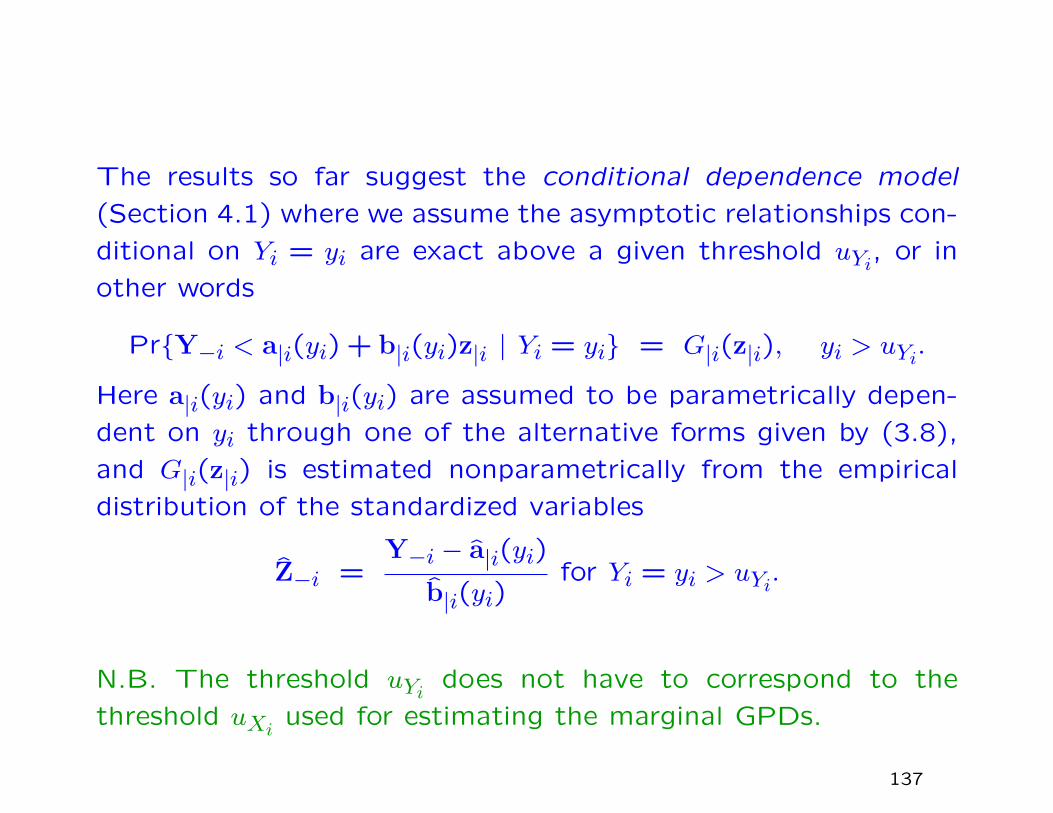
The results so far suggest the conditional dependence model
(Section 4.1) where we assume the asymptotic relationships con-
ditional on Yi = yi are exact above a given threshold uYi, or in
other words
Pr{Y−i < a|i(yi) + b|i(yi)z|i | Yi = yi} = G|i(z|i), yi > uYi.
Here a|i(yi) and b|i(yi) are assumed to be parametrically depen-
dent on yi through one of the alternative forms given by (3.8),
and G|i(z|i) is estimated nonparametrically from the empirical
distribution of the standardized variables
Z−i =Y−i − a|i(yi)
b|i(yi)for Yi = yi > uYi.
N.B. The threshold uYi does not have to correspond to the
threshold uXi used for estimating the marginal GPDs.
137

Some issues raised by this representation:
• Self-consistency of separate conditional models? (Section
4.2)
• Extrapolation — critical to have parametric forms for a|i(yi)and b|i(yi) (Section 4.3)
• Diagnostics — combine standard diagnostics for marginal
extremes with tests of independence of Z−i and Yi. Also test
whether the separate components of Z−i are independent,
since estimation via empirical distribution is much simpler in
this case.
138

Inference
1. Estimation of marginal parameters
If ψ denotes the collection of all (βi, ξi) parameters for the indi-vidual GPDs, maximize
logL(ψ) =d∑
i=1
nuXi∑k=1
log fXi(xi|i,k)
Here nuXiis the number of threshold exceedances in the i’th
component and fXi(xi|i,k) is the GP density evaluated at thek’th exceedance.
[In essence, if there is no functional dependence among the(βi, ξi) for different i then this is just the usual marginal estima-tion of the GPD in each component. But if there is functionaldependence, we estimate the parameters jointly by combining theindividual likelihood estimation equations, ignoring dependenceamong the components.]
139

2. Single conditional
i.e. How do we estimate a|i(yi) and b|i(yi) for a single i, assumingparametric representation?
The problem: don’t know the distribution of Z|i.
The solution: do it as if the Z|i were Gaussian with known meansµµµ|i and standard deviations σσσ|i
This leads to the formulae
µµµ|i(y) = a|i(y) + µµµ|ib|i(y),
σσσ|i(y) = σσσ|ib|i(y),
and estimating equation
Qi = −∑j 6=i
nuYi∑k=1
logσj|i(yi|i,k) +1
2
yj|i,k − µj|i(yi|i,k)
σj|i(yi|i,k)
2 .140
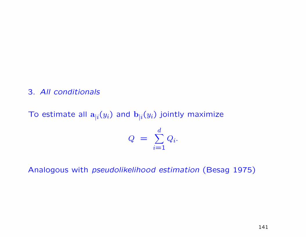
3. All conditionals
To estimate all a|i(yi) and b|i(yi) jointly maximize
Q =d∑
i=1
Qi.
Analogous with pseudolikelihood estimation (Besag 1975)
141

4. Uncertainty
Bootstrap.....
142

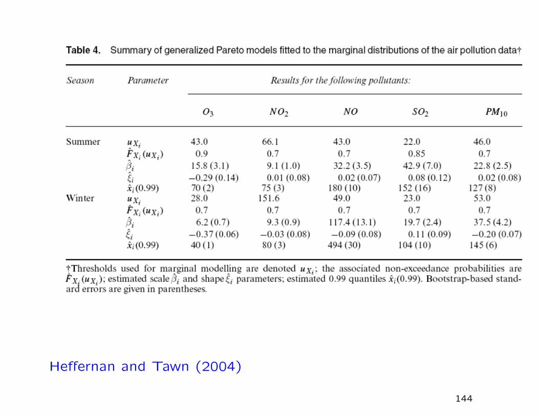
Air quality application
The data: daily values of five air pollutants (O3, NO2, NO, SO2,
PM10) in Leeds, U.K., during 1994–1998.
Two seasons: winter (NDJF), early summer (AMJJ)
Omit values around November 5 and some clear outliers
Marginal model: fit GPD above a (somewhat) high threshold,
estimate 99% quantile with standard error (Table 4)
143
Heffernan and Tawn (2004)
144

Dependence model
Transform margins to Gumbel, select threshold for dependencemodeling. Selected to be 70% quantile (for all five variables)
Estimate (aj|i, bj|i) and (ai|j, bi|j) for each combination of i 6=j, with sampling variability represented by convex hull of 100bootstrap simulations (Fig. 5).
Several pairs do not exhibit weak pairwise exchangeability (e.g.PM10, O3 in summer)
Components of Z|i are typically dependent
Some pairs exhibit negative dependence (e.g. O3, NO in winter— consistent with chemical reactions)
Fig. 6 shows pseudosamples of other variables given NO overthreshold (C5(23) are points for which sum of all 5 variables onGumbel scale exceeds 23)
145

Heffernan and Tawn (2004)
146

Heffernan and Tawn (2004)
147
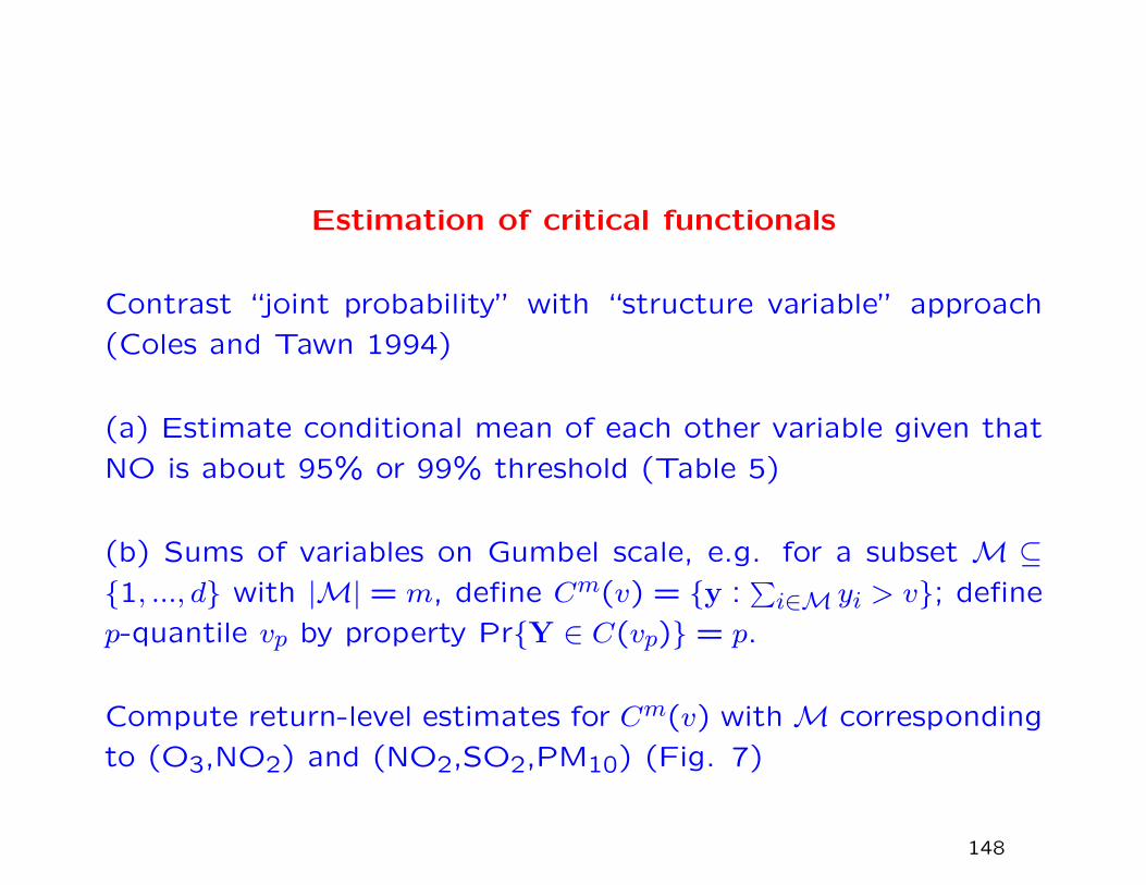
Estimation of critical functionals
Contrast “joint probability” with “structure variable” approach
(Coles and Tawn 1994)
(a) Estimate conditional mean of each other variable given that
NO is about 95% or 99% threshold (Table 5)
(b) Sums of variables on Gumbel scale, e.g. for a subset M ⊆{1, ..., d} with |M| = m, define Cm(v) = {y :
∑i∈M yi > v}; define
p-quantile vp by property Pr{Y ∈ C(vp)} = p.
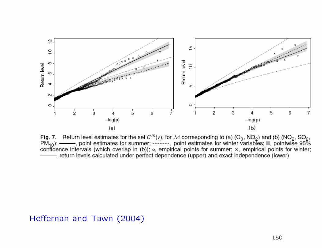
Compute return-level estimates for Cm(v) with M corresponding
to (O3,NO2) and (NO2,SO2,PM10) (Fig. 7)
148

Heffernan and Tawn (2004)
149
Heffernan and Tawn (2004)
150
Further work on the Heffernan-Tawn model
See in particular
J.E. Heffernan and S.I. Resnick (2007), Limit laws for random
vectors with an extreme component. Annals of Applied Proba-
bility 17, 537–571
for a detailed analysis of the probability theory underlying the
Heffernan-Tawn method. This should eventually lead to new
statistical methods, though that has still to be done!
151

VII.3 MAX-STABLE PROCESSES
152

A stochastic process {Zt, t ∈ T}, where T is an arbitrary index
set, is called max-stable if there exist constants ANt > 0, BNt(for N ≥ 1, t ∈ T ) with the following property: if Z(1)
t , ..., Z(N)t
are N independent copies of the process and
Z∗t =
(max
1≤n≤NZ
(n)t −BNt
)/ANt, t ∈ T,
then {Z∗t , t ∈ T} is identical in law to {Zt, t ∈ T}.
WLOG, assume margins are Unit Frechet,
Pr{Zt ≤ z} = e−1/z, for all t (5)
in which case ANt = N, BNt = 0. Note that even though this
assumption may be made for the purpose of characterizing the
stochastic process, we would still have to estimate the marginal
distributions in practice.
153

Construction of Max-Stable Processes
Let {(ξi, si), i ≥ 1} denote the points of a Poisson process on(0,∞) × S with intensity measure ξ−2dξ × ν(ds), where S is anarbitrary measurable set and ν a positive measure on S. Let{f(s, t), s ∈ S, t ∈ T} denote a non-negative function for which∫
Sf(s, t)ν(ds) = 1, for all t ∈ T (6)
and define
Zt = maxi{ξif(si, t)}, t ∈ T. (7)
“Rainfall-storms” interpretation: S is space of “storm centres”,ν as a measure representing distribution of storms over S. Eachξi represents the magnitude of a storm, and ξif(si, t) representsthe amount of rainfall at position t from a storm of size ξi centredat si; the function f represents the “shape” of the storm. Themax operation in (7) represents the notion that the observedmaximum rainfall Zt is a maximum over independent storms.
154

Fix zt > 0 for each t, and consider the set
B = {(ξ, s) : ξf(s, t) > zt for at least one t ∈ T}.
The event {Zt ≤ zt for all t} occurs if and only if no points ofthe Poisson process lie in B. However, the Poisson measure ofthe set B is∫
S
∫ ∞0
I
{ξ > min
zt
(f(s, t)
}ξ−2dξ ν(ds) =
∫S
maxt
{f(s, t)
zt
}ν(ds)
where I is the indicator function, and consequently
Pr{Zt ≤ zt for all t} = exp
[−∫S
maxt
{f(s, t)
zt
}ν(ds)
]. (8)
It follows from (8) and (6) that the marginal distribution of Zt,for any fixed t, is of Frechet form (5), and by direct verificationfrom (8), the process is max-stable.
155
Examples (Smith 1990)
Multivariate normal form:
Suppose S = T = <d, ν is Lebesgue measure, and
f(s, t) = f0(s− t) = (2π)−d/2|Σ|−1 exp{−
1
2(s− t)TΣ−1(s− t)
}.
Formula for Pr{Yt1 ≤ y1, Yt2 ≤ y2} is
exp
{−
1
y1Φ
(a
2+
1
alog
y2
y1
)−
1
y2Φ
(a
2+
1
alog
y1
y2
)}where Φ is the standard normal distribution function and
a2 = (t1 − t2)TΣ−1(t1 − t2).
156

Pickands dependence function:
A(w) = (1− w)Φ(a
2+
1
alog
1− ww
)+ wΦ
(a
2+
1
alog
w
1− w
).
Limits a → 0 and a → ∞ become the extreme cases A(w) =
max(w,1 − w) and A(w) = 1 representing, respectively, perfect
dependence and independence.
Note that A(
12
)= Φ
(a2
).
Remark. This dependence function was independently derived
by Husler and Reiss (1989) as a limiting form for the joint distri-
bution of bivariate extremes from a bivariate normal distribution
with correlation ρn varying with sample size n, in such a way
that n→∞, ρn → 1 and (1− ρn) logn→ a2/4. They also gave a
multivariate extension.
157

Multivariate t form:
f0(x) = |Σ|−1/2(πv)−d/2 Γ(v/2)
Γ((v − d)/2)
(1 +
xTΣ−1x
v
)−v/2
,
valid for all x ∈ <d, where Σ is again a positive definite covariancematrix and v > d.
No general formula for even the bivariate joint distributions, butwe do have
A
(1
2
)=
1
2
{1 +B
(a2
a2 + 4v2;
1
2,v − d
2
)},
where a =√
(t1 − t2)TΣ−1(t1 − t2) again and B is the incompletebeta function,
B(y;α, β) =Γ(α+ β)
Γ(α)Γ(β)
∫ y0uα−1(1− u)β−1du, 0 ≤ y ≤ 1.
Note that, as v →∞, A(1/2)→ Φ(a/2) which is consistent withthe MVN case.
158

Representations of Max-Stable Processes
The representation (8) first appeared in a number of papers
in the 1980s, such as de Haan (1984), de Haan and Pickands
(1986), Gine, Hahn and Vatan (1990).
However it is not the most general representation, as shown in
particular by Schlather (2002).
159
Schlather’s First Representation
Let Y be a measurable random function on <d,µ = E
{∫<d max(0, Y (x))dx
}∈ (0,∞), Π a point process on <d ×
(0,∞) with intensity measure dΛ(y, ξ) = µ−1dyξ−2dξ,
Z(x) = sup(ξ,y)∈Π
ξYy,ξ(x− y),
where each Yy,ξ(·) is an independent copy of Y .
Then Z is max-stable with unit Frechet margins.
160

Schlather’s Second Representation
Let Y be a stationary process on <d,µ = E {max(0, Y (x))} ∈ (0,∞), Π a point process on (0,∞) with
intensity measure µ−1ξ−2dξ,
Z(x) = maxξ∈Π
ξYξ(x) = maxξ∈Π
max{0, ξYξ(x)},
where each Yξ(·) is an independent copy of Y .
Then Z is max-stable with unit Frechet margins.
161
Example:
Suppose Y is a stationary standard normal random field with
correlation function ρ(t). Let Π be a Poisson process on (0,∞)
with intensity measure dΛ(ξ) =√
2πξ−2dξ. Then the process
Z(s) = maxξ∈Π max{0, ξYξ(s)} defines an extremal Gaussian pro-
cess. Its bivariate distributions satisfy
Pr{Z(s1) ≤ x1, Z(s2) ≤ x2}
= exp
{−
1
2
(1
x1+
1
x2
)(1 +
√1− 2(ρ(s1 − s2)− 1)
x1x2
(x1 + x2)2
)},
Another new class of bivariate EVDs!
162

Statistical Methods
Smith (1990)
Coles (1993)
Coles and Tawn (1996)
Buishand, de Haan and Zhou (2008)
Naveau, Guillou, Cooley and Diebolt (2009)
163

Method of Smith (1990)
Define the extremal coefficient between two variables: if X1 and
X2 have same marginal cdf F (·),
Pr{X1 ≤ x, X2 ≤ x} = F θ(x).
In BEVD case, θ = 2A(
12
).
Remark. Various people have proposed the extension where
F θ(x) is replaced by F θ(x)(x), θ(x) depending on the level x.
In some contexts, this could be equivalent to the Ledford-Tawn
representation.
164
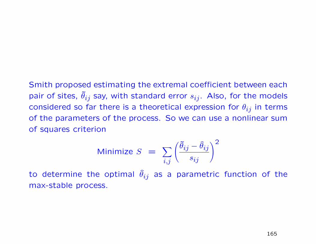
Smith proposed estimating the extremal coefficient between each
pair of sites, θij say, with standard error sij. Also, for the models
considered so far there is a theoretical expression for θij in terms
of the parameters of the process. So we can use a nonlinear sum
of squares criterion
Minimize S =∑i,j
(θij − θijsij
)2
to determine the optimal θij as a parametric function of the
max-stable process.
165
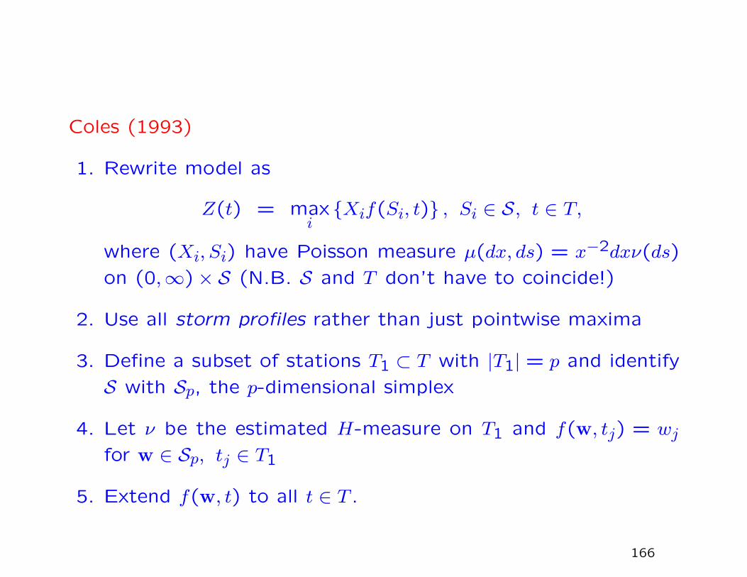
Coles (1993)
1. Rewrite model as
Z(t) = maxi{Xif(Si, t)} , Si ∈ S, t ∈ T,
where (Xi, Si) have Poisson measure µ(dx, ds) = x−2dxν(ds)
on (0,∞)× S (N.B. S and T don’t have to coincide!)
2. Use all storm profiles rather than just pointwise maxima
3. Define a subset of stations T1 ⊂ T with |T1| = p and identify
S with Sp, the p-dimensional simplex
4. Let ν be the estimated H-measure on T1 and f(w, tj) = wjfor w ∈ Sp, tj ∈ T1
5. Extend f(w, t) to all t ∈ T .
166

Coles and Tawn (1996)
Objective: calculate extremal distributions of areal averages basedon point rainfall data
Method:
1. Focus on i’th rain event with precipitation Xi(v), v ∈ V
2. Unit Frechet Transformation Ψv(Xi(v)) = Xi(v) after fitting(mu(v), ψ(v), ξ(v)) GEV model to each site v
3. Write Xi(v) = ξif(si, v) using point process representation ofColes (1993), fitted to storms for which at least one Xi(v)exceeded some high threshold
4. Area average
Yi =1
∆V
∫V
Ψ−1v (ξif(si, v))dv.
167

Naveau, Guillou, Cooley and Diebolt (2009)
Define madogram: if M(x), x ∈ X is a stationary process of
pointwise maxima over some space X, with marginal cdf F , then
ν(h) =1
2E {|F (M(x+ h))− F (M(x))|} .
In particular, the extremal coefficient between two sites x and
x+ h is 1+2ν(h)1−2ν(h) .
Disadvantage: only relevant to joint probabilities Pr{M(x) ≤u, M(x+ h) ≤ v} in cases u = v.
168

The λ-madogram:
ν(h, λ) =1
2E{∣∣∣Fλ(M(x+ h))− F1−λ(M(x))
∣∣∣} .Then the exponent measure V is
V (λ,1− λ) =c(λ) + ν(h, λ)
1− c(λ)− ν(h, λ),
where c(λ) = 3/{2(1 + λ)(2− λ)}, λ ∈ (0,1).
If we assume the marginal cdf is known, then the estimator of
ν(h, λ) is obvious. The main focus of the paper of Naveau et
al. (2009) is to estimate ν(h, λ) when the marginal distribu-
tion is unknown. They do this nonparametrically using empirical
process theory. This is an alternative to the Smith-Tawn-Coles
method of estimating the distribution above a high threshold via
GEV/GPD approximations.
169

Buishand, de Haan and Zhou (2008)
This will be Zhitao Zhang’s class presentation. Therefore, I omit
any discussion here, except to say that it is closely related to the
methods of the previous papers.
170

Other (recent) books on extremes
1. Coles (2001)
Best overall introduction to the whole subject
2. Finkenstadt and Rootzen (editors) (2003)
Proceedings of European conference: includes RLS overview
chapter, and Fougeres on multivariate extremes
3. Beirlant, Goegebeur, Segers and Teugels (2004)
Comprehensive overview of traditional extreme value theory,
including multivariate extremes
4. De Haan and Ferreira (2006)
Particular focus on max-stable ideas
5. Resnick (2007)
Different focus: focus on probability models but including
relevant statistics
171

REFERENCES
172

Beirlant, J., Goegebeur, Y., Segers, J. and Teugels, J. (2004),
Statistics of Extremes: Theory and Appications Wiley Series in
Probability and Statistics, Chichester, U.K.
Besag, J.E. (1975), Statistical analysis of non-lattice data.
The Statistician 24, 179–195.
Buishand, T.A., de Haan, L. and Zhou, C. (2008), On spa-
tial extremes: with application to a rainfall problem. Annals of
Applied Statistics 2, 624–642.
Coles, S.G. (1993), Regional modelling of extreme storms via
max-stable processes. JRSSB 55, 797–816.
Coles, S.G. (2001), An Introduction to Statistical Modeling
of Extreme Values. Springer Verlag, New York.
Coles, S.G. and Tawn, J.A. (1991), Modelling extreme multi-
variate events. J.R. Statist. Soc. B 53, 377–392.
Coles, S.G. and Tawn, J.A. (1994), Statistical Methods for
Multivariate Extremes: An Application to Structural Design (with
discussion). Applied Statistics 43, 1–48.
173

Coles, S.G. and Tawn, J.A. (1996), Modelling extremes of
the areal rainfall process. JRSSB 58, 329–347.
Cooley, D., Nychka, D. and Naveau, P. (2007), Bayesian spa-
tial modeling of extreme precipitation return levels. Journal of
the American Statistical Association 102, 824–840.
Finkenstadt, B. and Rootzen, H. (editors) (2003), Extreme
Values in Finance, Telecommunications and the Environment.
Chapman and Hall/CRC Press, London.
Gine, E., Hahn, M. and Vatan, P. (1990), Max infinitely di-
visible and max stable sample continuous processes. Probab.
Theor. and Relat. Fields 87, 139–165.
Groisman, P.Ya, Knight, R.W., Easterling, D.A., Karl, T.R.,
Hegerl, G.C. and Razuvaev, V.N. (2005), Trends in intense pre-
cipitation in the climate record. Journal of Climate 18, 1326–
1350.
Gumbel, E.J. and Goldstein, N. (1964), Analysis of empirical
bivariate extremal distributions. J. Amer. Statist. Soc. 59,
794–816.
Haan, L. de (1984), A spectral representation for max-stable
processes. Ann. Probab. 12, 1194-1204.
174

Haan, L. de and Pickands, J. (1986), Stationary min-stable
stochastic processes. Prob. Th. Rel. Fields 72, 477-492.
Husler, J. and Reiss, R.-D. (1989), Maxima of normal ran-
dom vectors: Between independence and complete dependence.
Statistics and Probability Letters 7, 283-286.
Haan, L. de and Ferreira, A. (2006), Extreme Value Theory:
An Introduction. Springer Series in Operations Research and Fi-
nancial Engineering, New York.
Heffernan, J.E. and Resnick, S. (2005), Hidden regular vari-
ation and the rank transform. Advances in Applied Probabilitty
37-2, 393–414.
Heffernan, J.E. and Resnick, S. (2007), Limit laws for random
vectors with an extreme component. Annals of Applied Proba-
bility 17, 537–571
Heffernan, J.E. and Tawn, J.A. (2004), A conditional ap-
proach for multivariate extreme values. J.R. Statist. Soc. B 66,
497–546 (with discussion)
Joe, H. (1990), Families of min-stable multivariate exponen-
tial and multivariate extreme value distributions. Statist. and
Probab. Letters 9, 75–81.
175

Ledford, A.W. and Tawn, J.A. (1996), Modelling dependence
within joint tail regions, J.R. Statist. Soc. B 59, 475–499
Ledford, A.W. and Tawn, J.A. (1997), Statistics for near in-
dependence in multivariate extreme values. Biometrika 83, 169–
187.
Mannshardt-Shamseldin, E.C., Smith, R.L., Sain, S.R., Mearns,
L.O. and Cooley, D. (2008), Downscaling extremes: A compar-
ison of extreme value distributions in point-source and gridded
precipitation data. Preprint, under revision.
Maulik, K. and Resnick, S. (2005), Characterizations and ex-
amples of hidden regular variation. Extremes 7, 31–67
Naveau, P., Guillou, A., Cooley, D. and Diebolt, J. (2009),
Modelling pairwise dependence of maxima in space. Biometrika
96, 1–17.
Ramos, A. and Ledford, A. (2009), A new class of models for
bivariate joint tails. J.R. Statist. Soc. B 71, 219–241.
Ramos, A. and Ledford, A. (2008), An alternative point pro-
cess framework for modeling multivariate extreme values. Preprint.
Resnick, S. (1987), Extreme Values, Point Processes and Reg-
ular Variation. Springer Verlag, New York.
176
Resnick, S. (2002), Second order regular variation and asymp-
totic independence. Extremes 5, 303–336
Resnick, S. (2007), Heavy-Tail Phenomena: Probabilistic and
Statistical Modeling. Springer, New York.
Robinson, M.E. and Tawn, J.A. (1995), Statistics for excep-
tional athletics records. Applied Statistics 44, 499–511.
Sang, H. and Gelfand, A.E. (2008), Hierarchical modeling for
extreme values observed over space and time. Published online
by Environmental and Ecological Statistics.
Schlather, M. (2002), Models for Stationary Max-Stable Ran-
dom Fields. Extremes 5(1), 33–44.
Shi, D. (1995), Fisher information for a multivariate extreme
value distribution. Biometrika 82, 644–649.
Smith, R.L. (1989), Extreme value analysis of environmental
time series: An application to trend detection in ground-level
ozone (with discussion). Statistical Science 4, 367–393.
Smith, R.L. (1990), Max-stable processes and spatial ex-
tremes. Unpublished, available from
http://www.stat.unc.edu/postscript/rs/spatex.pdf
177
Smith, R.L. (1997), Statistics for exceptional athletics records.
Letter to the Editor, Applied Statistics 46, 123–127.
Smith, R.L. (2003), Statistics of extremes, with applica-
tions in environment, insurance and finance. Chapter 1 of Ex-
treme Values in Finance, Telecommunications and the Environ-
ment, edited by B. Finkenstadt and H. Rootzen, Chapman and
Hall/CRC Press, London, pp. 1–78.
Smith, R.L. and Goodman, D. (2000), Bayesian risk analy-
sis. Chapter 17 of Extremes and Integrated Risk Management,
edited by P. Embrechts. Risk Books, London, 235-251.
Smith, R.L. and Weissman, I. (1994), Estimating the extremal
index. J.R. Statist. Soc. B 56, 515–128.
Stott, P.A., Stone, D.A. and Allen, M.R. (2004), Human
contribution to the European heatwave of 2003. Nature 432,
610–614 (December 2 2004)
Tawn, J.A. (1990), Modelling multivariate extreme value dis-
tributions. Biometrika 77, 245–253.
178