F-MStorm: Feedback-based Online DistributedMobile Stream Processing

Mengyuan Chao, Chen Yang, Yukun Zeng, Radu StoleruTexas A&M University, USA

Email: {chaomengyuan, yangchen08, yzeng}@tamu.edu; stoleru@cse.tamu.edu

Abstract—A distributed mobile stream processing system al-lows mobile devices to process stream data that exceeds any singledevice’s computation capability without the help of infrastruc-ture. It is paramount to have such a system in many criticalapplication scenarios, such as military operations and disasterresponse, yet an efficient online mobile stream processing systemis still missing. In this paper, we make the key observation thatthe unique characteristics of mobile stream processing call for afeedback-based system design, which is in sharp contrast with thestatic configuration and scheduling of the current mobile streamprocessing system, “MStorm” [1]. At first, we demonstrate theinefficiencies of MStorm through several real-world experiments.Then, we propose F-MStorm, a feedback-based online distributedmobile stream processing system, which adopts the feedback-based approach in the configuration, scheduling and executionlevels of system design. We implement F-MStorm on Androidphones and evaluate its performance through benchmark appli-cations. We show that it achieves up to 3x lower response time,10% higher throughput and consumes 23% less communicationenergy than the state-of-the-art systems.

Index Terms—stream processing; edge computing; scheduling

I. INTRODUCTION

Emerging computation-intensive mobile applications [2]–[7]that process stream data collected by various mobile sensorsoften require more computation resources than a single devicecan provide. Therefore, many existing systems [8]–[10] offloadthe computation-intensive tasks to the cloud or nearby highperformance computing (HPC) servers to achieve low latency.For example, MCDNN [8] offloads deep neural network basedvideo processing tasks to the cloud, Odessa [9] chooses nearbyHPCs as additional computing resources to recognize objectsfrom real-time videos and LEO [10] utilizes on-chip DSP co-processors, GPUs together with the cloud to run inferencealgorithms. Although such systems achieve low latency andhigh throughput, resources in the cloud or nearby HPC serversare not always accessible in some infrastructure-less scenarios.For example, imagine the following scenario:

“A group of first responders, equipped with mobile devices,is assigned to a post-earthquake area to discover dangerouszones (e.g., leaking chemical pipes or unstable buildings)to avoid. The teams collect a large amount of data viadifferent sensors (e.g., on body video cameras) and analyzethe data in real time via analytical software. Usually, suchdata analysis requires significant computational resourcesand, thus, it is pushed to the cloud for analysis. However,the communication infrastructure was destroyed during theearthquake, which makes offloading to the cloud impossible.In such case, offloading computation to the nearby mobiledevices at the edge becomes a promising option.”

In this paper, we focus on a distributed stream processingsystem deployed on a cluster of mobile devices without anInternet access (stream processing at the edge). Differentfrom most stream processing systems that run on a clusterof wire-connected servers in the cloud (such as Storm [11],Spark [12] and Flink [13], etc.), stream processing on acluster of mobile devices is much more complicated, becausemobile devices have very limited computation resources andbatteries, and the wireless links between different devices areunstable. Some existing works [14], [15] are designed for thesame environment as ours. However, they focus on processingbounded batch jobs instead of unbounded stream data.

MStorm [1] makes an important first step towards mobilestream processing at the edge by implementing a lightweightsystem on mobile phones. It provides some basic functionality,such as parallelism configuration, task scheduling and streamgrouping. However, since its current implementation ignoressome specific characteristics of stream processing at the edge,it is inefficient as we demonstrate through some simple ex-periments. First, MStorm configures the number of executors(threads that execute tasks) at each device simply based onCPU cores while not taking into account the current CPUutilization. As the computation resources of a mobile deviceis also shared by other applications, this static configurationcan easily lead to a bottleneck that negatively impacts thesystem performance (response time and throughput). Second,the task assignment, when MStorm assigns computation tasksto devices, is based on a naive round robin strategy. This mayincur unnecessary inter-device traffic and consequently higherdelay and energy consumption. Third, MStorm adopts a shufflestream grouping mechanism, where upstream tasks distributethe output to downstream tasks uniformly at random. However,as downstream tasks may run on highly occupied devices, theshuffle grouping mechanism might cause congestion there andlead to high response time and low throughput.

To solve these problems, one potential solution is to carveout some static resources dedicated for stream processing [16].However, unlike servers in the cloud, the resources of mobiledevices at the edge are very limited and need to be shared withsome other resource-intensive applications. It is unreasonableto allow MStorm to take up some resources even when there isno stream processing tasks. Another approach is to apply a pullmodel [17], [18] like most modern cloud computing systems,where the machines ask for tasks when they have free slots.However, this model is not enough for stream processing atthe edge as it does not consider other factors like device-to-device delays and remaining batteries of devices. Our insightis that, instead of adopting an open-loop task scheduling whichassumes a static environment, a feedback-based approach that

273

2018 Third ACM/IEEE Symposium on Edge Computing

978-1-5386-9445-9/18/$31.00 ©2018 IEEEDOI 10.1109/SEC.2018.00027

(a) MStorm Architecture (b) Zookeeper directory

Fig. 1: MStorm system architecture

makes decisions based on the changing system state should beutilized to deal with the dynamic environment at the edge.

To accomplish this goal, we propose F-MStorm, a feedback-based online distributed mobile stream processing system. F-MStorm adopts a feedback-based approach at many differentlevels of system design so that the system can adapt quickly tothe changing environment to achieve high performance. At theconfiguration level, F-MStorm configures the number of ex-ecutors on each mobile device based on the free CPU resourcesof mobile devices and CPU usage of tasks. At the schedulinglevel, F-MStorm assigns tasks to mobile devices based on thetask-to-task traffic and device-to-device communication delayand energy consumption. At the execution level, the upstreamtasks distribute the output data to the downstream tasks basedon the latter’s stream arrival/processing rate and waiting queuelength. We implement a prototype of F-MStorm on Androidphones and evaluate its performance through a customizablebenchmark application. We also compare F-MStorm with twoscheduling algorithms proposed for Storm (i.e., T-Storm [19]and R-Storm [20]). The experimental results show that, byusing the feedback information, F-MStorm achieves up to 3xlower response time, 10% higher throughput and 23% lesscommunication energy than the state-of-the-art systems.

Our main contributions are summarized as follows:

• Through some real world experiments, we demonstratethat, without an accurate estimation of the current systemstate and appropriate adjustment of the initial configura-tion, task scheduling and stream grouping, MStorm suf-fers up to three order of magnitude increase in responsetime and 60% reduction in throughput (Section II), whichcalls for the feedback-based system design.

• We propose F-MStorm (Section III), which consists of afeedback-based configuration (FBC) method, a feedback-based task assignment (FBA) algorithm and a feedback-based stream grouping (FBG) strategy.

• We implement F-MStorm on Android phones and conductreal world experiments to evaluate its performance (Sec-tion IV), which demonstrate the superiority of F-MStormover MStorm and two other state-of-the-art systems.

II. BACKGROUND AND MOTIVATION

In this section, we at first briefly introduce the backgroundof MStorm and its architecture. Then, we show the inefficiencyof MStorm via three experiments. Finally, we motivate our F-MStorm by explaining why existing solutions do not work.

(a) Topology example

(b) Extended topology example

Fig. 2: Example of an MStorm application

A. MStorm

MStorm [1] is the first online distributed stream processingsystem running on mobile devices with Android OS. It isdesigned for critical scenarios such as military operationsand disaster response, where no Internet access is available,whereas the mobile devices of the team members are con-nected as a cluster through a manpack Wi-Fi access point.Instead of porting popular stream processing systems (such asStorm [11], Spark [12] or Flink [13]) running on the cloud,MStorm is designed and implemented from scratch with alightweight infrastructure. This is paramount for mobile streamprocessing at the edge, which only has limited resources.

MStorm adopts some technical designs from Apache Storm.Its architecture is shown in Fig. 1a. An MStorm master nodecontains one Nimbus and one Zookeeper service. Nimbusschedules task execution while Zookeeper coordinates betweenNimbus and mobile devices and maintains the cluster metadatain a directory-like structure shown in Fig. 1b. Every mobiledevice in the MStorm cluster runs a supervisor process anda worker process, both as Android services. The supervisorreceives tasks from Nimbus and assigns tasks to the worker,while the worker manages multiple executors (threads) whichare used to execute tasks. MStorm guarantees an at-most-onceprocessing semantics.

An application in MStorm is modeled as a directed graphcalled topology. A topology contains two types of nodes, i.e.,spout and bolt. A spout partitions the input stream into tuplesand sends these tuples to downstream bolts. A bolt processestuples from spout or upstream bolts, and sends the processedtuples to downstream bolts for further processing. We referto a spout or a bolt as application component (or simplycomponent) in the rest of the paper. A directed edge betweentwo nodes in a topology indicates that traffic flows from one tothe other. Each component can spawn multiple parallel taskswhich are executed by devices’ executors. If we expand thecomponent in a topology with multiple nodes, each of whichrepresents an individual task, we get another directed graph,i.e., the extended topology. The extended topology graphshows the actual data flow between individual tasks. Fig. 2shows the topology and the extended topology of a sampleMStorm application that contains one spout and two bolts,i.e., bolt1, bolt2. Each bolt further contains two parallel tasks,i.e., T2, T3 for bolt1, and T4, T5 for bolt2, respectively.

The MStorm application developer needs to provide theapplication topology as well as configure the parallel tasks foreach application component. MStorm then decides the numberof executors for each device and assigns tasks to devices forexecution. The output tuples of each task may need to besent to the downstream tasks. The mechanism for distributingtuples is called stream grouping. MStorm currently adopts a

274

Fig. 3: Sample application that demonstrates the inefficiency ofresource-unaware configuration and stream grouping

100

101

102

103

104

105

106

0 25 50 75 100 125 150 175 200 225 250

Avg

Del

ay (

ms)

Running Time (s)

T1T2

T3T4

(a) Delay

0 2 4 6 8

10 12 14 16 18

0 25 50 75 100 125 150 175 200 225 250

Thr

ough

put (

T/s

)

Running Time (s)

T1T2

T3T4

(b) Throughput

Fig. 4: The results of the sample application that demonstrates poorperformance of resource-unaware configuration

shuffle grouping strategy, i.e., tuples are randomly distributedto downstream tasks such that all tasks have identical expectedworkload in the long run.

B. Limitation of MStorm

Although MStorm makes an important first step towards asuccessful design of a mobile distributed stream processingsystem, its unawareness of system resource utilization andmobile network’s characteristics lead to the suboptimal be-haviors that prevent it from achieving a good performance. Inthe following sections, we present three experiments that showthe inefficiency of the current MStorm system.

1) Resource-unaware configuration (RUC): We refer to theconfiguration as the users’ preference of parallelism for eachcomponent and the system’s initial configuration of the numberof executors at each device. In MStorm, the system configuresthe number of executors at each device based on its CPU cores.However, since users may run other applications on the mobiledevice, the available CPU resources depend not only on theCPU cores but also on the current utilization. Configuring thenumber of executors without an accurate estimation of currentresource utilization may lead to performance bottleneck, wherethe heavily-used nodes may be assigned identical number ofexecutors compared to the idle ones.

We demonstrate this inefficiency through a sample applica-tion shown in Fig. 3, which consists of 4 tasks (T1 - T4). FourGoogle Nexus 5 mobile devices M1 - M4 form a cluster andMStorm configures identical number of executors per node.Due to round robin task assignment, which we discuss later,as it is also inefficient, each mobile device needs to executeone task. Consider the case when M2 is actively used by otheruser’s application, MStorm fails to adapt to this situation andresults in poor performance as shown in Fig. 4. We generate astream of data at 12 tuples per second (T/s) and measure thedelay and throughput of each task. As we can see, the delay forT2 increases from 100ms to 100s because of queuing after thesystem runs for 250s. This is unacceptable for any real-timemobile application. Besides, the overall throughput (10T/s) issmaller than the input rate (12T/s) due to the bottleneck at T2.This leads to increasing queues in the system.

Fig. 5: The inter-device traffic incurred by different scheduling

2) Traffic-unaware task assignment: As mentioned earlier,MStorm uses a round robin task assignment strategy, i.e., itsequentially assigns tasks to each mobile device until all tasksare assigned. Although it is easy to implement, it does notminimize the inter-device traffic, which leads to a higher delayand energy consumption. To reduce the inter-device traffic,an intuitive idea is to put as many tasks as possible on thesame node. This leads to our two preliminary attempts for amore efficient task scheduling algorithm, namely breadth anddepth-first scheduling, respectively. The breadth (depth) firstscheduling works as follows: at first, sort the mobile devicebased on the number of configured executors; then assign tasksto the same mobile device in a breadth (depth) first orderwhen traversing the extended topology, until the assigned tasksreach its capacity or there is no more task to assign. However,we reveal by the following example that, even if the breadth(depth) first scheduling reduces some inter-device traffic, theirperformance are still much worse than the optimal schedule.

Fig. 5 (a) and (b) represent the topology and extendedtopology of an application. The edge weights in the extendedtopology represent the total traffic from task to task duringa period ΔT . All tasks are assigned to mobile devices M1,M2, M3, M4 with 3, 2, 1, 1 executors by different schedulingalgorithms. Based on the breadth/depth-first scheduling, tasksare assigned to mobile devices as shown in Fig. 5 (c)and (d). Figure (e) represents the optimal scheduling thatminimizes the inter-device traffic. Fig. 5 (f) summarizes thescheduling result and corresponding inter-device traffic foreach scheduling algorithm, which shows that the round robinscheduling generates 118% more inter-device traffic than theoptimal scheduling, whereas the breadth-first and depth-firstscheduling also generates 45%, 64% more inter-device trafficthan the optimal. This is because they fail to further distinguishdifferent inter-task traffic and don’t assign tasks with largeinter-task traffic to the same node.

Moreover, even if we distinguish different inter-task traffic,it is still coarse grained, considering the diversity of wirelesslinks. For example, given two tasks with fixed inter-task traffic,if they are assigned to two nodes with a lower inter-devicedelay, the total delay will be lower. If they are assigned totwo nodes with lower communication power, the total energyconsumption for traffic transmission will be less. With roundrobin or breadth (depth) first scheduling, all these potentialchances of improving system performance will be missed.

275

100

101

102

103

104

105

106

0 100 200 300 400 500 600 700 800 900 1000

Avg

Del

ay (

ms)

Running Time (s)

T1T2

T3T4

(a) Delay

0 2 4 6 8

10 12 14 16 18

0 100 200 300 400 500 600 700 800 900 1000

Thr

ough

put (

T/s

)

Running Time (s)

T1T2

T3T4

(b) Throughput

Fig. 6: The results of the sample application that demonstrates poorperformance of resource-unaware shuffle grouping

Furthermore, except for minimizing delay and energy con-sumption, sometimes soldiers or first responders require thesystem to last longer. To achieve this goal, the tasks need to beassigned based on the remaining battery of each device. Withround robin or breadth (depth) first scheduling, the batteriesof some devices might be depleted very soon.

3) Resource-unaware stream grouping: Recall that MStormadopts a shuffle grouping strategy to distribute output tuples todownstream tasks. Although shuffle grouping achieves fairnessamong tasks in terms of overall workload, we demonstrate thatit cannot adapt to the resource fluctuation resulted from users’own application usage.

We use the same application as shown in Fig. 3, where allnodes are idle in the beginning. We set the input rate at 10T/s.We run resource-intensive applications on M2 and M3 at 500sand 50s, and close them at 600s and 170s, respectively. Sinceshuffle grouping assigns output tuples from T1 to T2 and T3uniformly at random, the arrival rate at T2 and T3 are 5T/s onaverage, even if M2 and M3 are busy with other applications.As a result, we can see a significant increase in response timein Fig. 6a (from roughly 102ms to 105ms) and a decrease inthroughput in Fig. 6b (from roughly 5T/s to 2T/s), when theresource-intensive application is running.

A key observation from Fig. 3 is that the throughput of T2and T3 increases to 6T/s and 8T/s after the resource-intensiveapplication terminates, which indicates a higher processingcapability than the average input rate of 5T/s. Therefore, it ispossible to improve the overall throughput by assigning morestream to other more capable nodes, given that we have anaccurate online estimation of resource utilization at each node.

C. Motivation of F-MStorm

One simple approach to solve the problems above is to carveout some static resources on each mobile device dedicated forstream processing [16]. However, unlike servers in the cloudthat are uniformly managed by a cluster manger to undertakespecific jobs, the limited resources of mobile devices at theedge are shared by both MStorm and other user applications.Those applications might also be resource-intensive and evenhave higher priorities. It is unreasonable to allow MStormto take up the valuable resources even when there is nostream processing tasks. Another approach is to apply apull model [17], [18] like most modern cloud computingsystems, where the machines ask for tasks when they havefree slots. However, this model is not enough for streamprocessing at the edge as it does not consider other factorslike device-to-device delays, energy consumption of inter-device communication and remaining batteries of devices. We

argue that, instead of adopting an open-loop task schedul-ing algorithm which assumes a rather static environment, afeedback-based approach which makes decisions based onthe current system state (such as CPU utilization, delays andenergy consumption of inter-device communication, remainingbatteries, etc.) should be utilized to deal with the dynamicenvironment at the edge. Two ameliorations proposed forApache Storm, namely T-Storm [19] and R-Storm [20], havesimilar insights with F-MStorm. They also adopt a feedback-based approach to improve the system performance. However,neither of them concerns the energy consumption and balanceof energy usage, as they are proposed for systems running inthe cloud. Nevertheless, for a mobile stream processing systemrunning at the edge, the above two factors directly decide howlong a system can last for. It is paramount for F-MStorm totake all these factors into account.

III. DESIGN AND IMPLEMENTATION OF F-MSTORM

In this section, we present the design and implementationof F-MStorm. To overcome the inefficiencies presented in theprevious section, F-MStorm sets configuration, task schedulingand stream grouping all based on the feedback information.To better present our idea, we use a scenario with m devicesand an application with N components. The mathematicalmodel of the problem involves many notations. For readers’convenience, we summarize them in Table I.

A. OverviewSimilar with MStorm, F-MStorm configures the parallelism

of each application component based on the user’s experienceand assigns tasks to the mobile devices through round robinat the beginning. Then, after a “warm-up” period, each mobiledevice periodically reports the feedback information, includingtask execution, device resources and network condition, etc., toNimbus. Based on this feedback, F-MStorm reconfigures tasksfor each component, resets available executors for each deviceand recalculates the best schedule for the whole application.Because of the dynamic processing workload and changingenvironment, the best task schedule might change from timeto time. However, the new best schedule sometimes onlyachieve a small performance improvement than the previousone. In such case, it is not beneficial to switch to the newschedule, considering the rescheduling overhead and systemstability. To deal with this issue, we propose several rescheduleconditions. If none of these conditions are met, the systemjust keeps the origin schedule; otherwise, the reschedule takesplace. Except for reporting to Nimbus, each downstream taskneeds to report the execution information to the upstream tasksperiodically. The upstream tasks then distribute the output tothe downstream tasks based on the feedback information.

B. Status ReportIn F-MStorm, each mobile device reports the following

information to Nimbus periodically (every ΔT ):

• wj : the CPU usage (in MHz) of task j obtained from/proc/stat and /proc/stat/pid/task/tid/stat [19].

• lj : the queue length at task j, i.e., the number of streamtuples that are waiting to be processed.

• λj and μj : the average input and processing rate (in T/s) oftask j during ΔT .

• tjj′ : the output rate (in T/s) from task j to j′ during ΔT .

276

TABLE I: Main notations

Notation Descriptioni Index of component, i = 1, ..., Nj Index of task, j = 1, ..., n. n varies with configurationsk Index of mobile device, k = 1, ...,m

A(i) Task set of component ic(j) Component that task j belongs tov(j) Device that task j is assigned toWi Expected CPU usage of component iIi Expected input rate of component iOi Expected output rate of component iwj CPU usage (MHz) of task jlj Waiting queue length at task jλj Input rate (T/s) of task jμj Processing rate (T/s) at task jtjj′ Output rate (T/s) from task j to j′sjj′ Average tuple size (bit) from task j to j′fk Single core frequency (MHz) of device kck The number of CPU cores of device kuk Total CPU usage (MHz) of device krk Available CPU resource (MHz) at device kdkk′ Communication delay (ms) from device k to k′bk Remaining battery at device ketk Energy consumption (nJ) per bit for Tx at device kerk Energy consumption (nJ) per bit for Rx at device kP Vector: parallel task number for each componentE Vector: available executors for each mobile deviceB Vector: remaining battery for each mobile deviceT Matrix: average output rate from task to taskS Matrix: average tuple size from task to taskD Matrix: communication delay from device to deviceQ Matrix: energy/bit for transmitting between devicesX Matrix: task assignment to mobile devicesΔT Period that mobile devices report to NimbusΔt Period that tasks report to upstream tasks

• sjj′ : the average tuple size (bit) from task j to j′ duringΔT . It is defined as the ratio between the total tuple datasize and the total number of tuples from task j to j′.

• rk: the available CPU resource (in MHz) at device k, definedas rk = fk · ck − (uk −

∑v(j)=k wj), where fk is the single

core frequency, ck is the number of cores, uk is the currentCPU usage at device k, and

∑v(j)=k wj is the total CPU

usage of current F-MStorm tasks at device k.• dkk′ : device-to-device communication delay (in ms) from

device k to k′.• bk: remaining battery (in mAh) at device k.• etk and erk: energy consumption per bit (nJ/bit) for tuple

transmission (Tx) and reception (Rx). They can be estimatedbased on throughput [21], which we obtained from Device-BandwidthSampler [22].

Nimbus maintains a moving average for each status, that is,V = δ∗Vold+(1−δ)∗Vnew, where Vold is the old value storedat Nimbus, Vnew is the new feedback value, and 0 ≤ δ ≤ 1 isa factor used to indicate how the status depends on the history.

It deserves to be mentioned that, periodically reportingand updating these system statuses might cause some extracommunication and computing overhead. However, comparedwith the communication traffic size and processing workloadof stream data, the overhead is negligible.

C. Feedback Based Configuration (FBC)Based on the feedback, Nimbus calculates the following

vectors to reconfigure the system: P = [Pi]Ni=1, E = [Ek]

mk=1.

Pi represents the number of parallel tasks of component i andEk represents the available executors of each mobile device k.

They are calculated by equation Pi = �Wi

R � and Ek = � rkR �,

where Wi is the expected CPU usage of component i, rk isthe available CPU resource at device k and R represents thecomputing resource of each executor. The ceiling and floorfunctions are used to leave some margins for device resourcefluctuation. R is calculated by the following equations:

⎧⎪⎨⎪⎩

R = min{max{Rl,Re},Ru}Rl = ηl ∗mink{fk}Re = mini,k{Wi,

rkck}

Ru = ηu ∗mink{fk}(1)

where ηl and ηu (0 ≤ ηl ≤ ηu ≤ 1) are parameters to controlthe lower and upper bound of an executor’s resource. Theintuitions are as follows. First, the resource of an executor ismostly determined by the CPU usage of components and theavailable resource of mobile devices. Based on this, we cancalculate a basic version of executor resource, namely Re.Then, to make full use of the CPU resource, a single executorshould not occupy more resource than a CPU core. Therefore,we need to set an upper bound Ru for the executor resource.On the other hand, the resource of an executor should notbe too little, otherwise a mobile device will be configuredwith too many executors, which incurs a lot of OS schedulingoverheads. Therefore, we also need to add a lower bound Rl

for the executor resource.

D. Feedback Based Assignment (FBA)

We formulate the task assignment in F-MStorm as a mixed-integer quadratic programming (MIQP) and solve it by agenetic algorithm. Moreover, to ensure the system stability, wepropose 4 reschedule conditions to avoid frequent reschedules.

1) Problem Formulation: Let matrix T = [Tjj′ ]n×n rep-resent the expected tuple output rate from task to task, with

Tjj′ = Ii/Pi∑j′ tjj′

∗ tjj′ , where i = c(j) is the component that

task j belongs to, Ii is the expected input rate of componenti. Ii/Pi represents the expected tuple input rate of each task.Let matrix S = [sjj′ ]n×n represent the measured averagetuple size from task to task and let matrix D = [dkk′ ]m×m

represent the communication delay between mobile devices.Let matrix Q = [Qkk′ ]m×m represent the energy per bit forcommunication from device k to k′, where Qkk′ = etk + erk′ .We denote the decision variables for the task assignment as an-by-m 0-1 matrix X , with Xjk = 1 representing that task jis assigned to device k.

Our objective is to minimize the average end-to-end delayand energy consumption for each tuple while ensuring theload balance in energy consumption. The end-to-end delayconsists of processing delay, queuing delay and communi-cation delay. The energy consumption consists of processingenergy and communication energy. Since the system we careis homogeneous in executor’s processing speed and energyconsumption model, the way we assign tasks will not affectthe end-to-end processing delay, queuing delay and processingenergy. Therefore, the objective is reduced to minimize theaverage end-to-end communication delay and communicationenergy consumption while ensuring the load balance in energyconsumption. We formulate the problem as:

minimizeX

F = α ∗ gdgmaxd

+ β ∗ gqgmaxq

+ γ ∗ gbgmaxb

(2)

277

s.t. ∀j,m∑

k=1

Xjk = 1

∀k,n∑

j=1

Xjk ≤ Ek

∀j, k, Xjk ∈ {0, 1}

(3)

where gd is the average communication delay, gq is the averagecommunication energy consumption and gb is the load balanceindex. gmax

d , gmaxq , gmax

b represent the maximum gd, gq and gbthat are used to unify the units. α, β, γ ∈ [0, 1] are customizedaccording to the user’s preference.

gd is calculated as follows. Given the task-to-task outputrate matrix T and task assignment matrix X , we can obtainmatrix T ′ = ΔT · TX , where element T ′

jk represents thetotal number of tuples output by j from device v(j) to kduring ΔT . Similarly, we can obtain matrix D′ = XD, whereelement D′

jk represents the communication delay from v(j)

to k. With T ′ and D′, we can obtain matrix Md = T ′D′,where element Md

jk represents the total communication delayof tuples output by task j from v(j) to k during ΔT , and represents Hadamard product. λ =

∑j∈A(1) μj represents the

total output rate of the spout. Then, the average communicationdelay of each tuple is calculated as:

gd =

∑j,k M

djk

λΔT=

∑j,k ΔT · (TX �XD)jk

λΔT

=

∑j,k(TX �XD)jk

λ

(4)

Next, we consider the calculation of gq . Similar to thecommunication delay, we utilize matrix T ′′ = ΔT ·(T S)Xto represent the total traffic data size output by task j fromdevice v(j) to k in ΔT , matrix Q′ = XQ to represent theenergy consumption per bit for tuple transmission by Wi-Fifrom device v(j) to k. Thereby, the total energy consumptionfor tuple transmission from device v(j) to k in ΔT can berepresented as matrix Mq = T ′′ Q′. Then, the power oftuple transmission is calculated as:

gq =

∑j,k M

qjk

ΔT=

∑j,k ΔT · ((T � S)X �XQ)jk

ΔT

=∑

j,k

((T � S)X �XQ)jk(5)

Finally, gb is calculated as follows:

gb =m∑

k=1

(n∑

j=1

Xjk − bk∑mk=1 bk

∗ n)2 (6)

where bk is the remaining battery of device k. The effect of thisitem is intuitive: when two devices posses the same availableCPU resources, the computation tasks should be assigned tothe one with more remaining battery to prolong the lifetimeof the whole system.

2) Genetic Algorithm-based Solution: The aforementionedproblem is typically solved by a CPLEX solver [23]. However,based on our experimental results, it takes 77 seconds onaverage to solve a moderately sized (e.g., 15 nodes and 15tasks) problem on a desktop, which is impractical for real timeapplications on mobile platforms. To deal with this issue, weimplement an approximation algorithm (Algorithm 1), whichreturns a near-optimal solution (within 5% of the optimal)

Algorithm 1: ApproxTaskSchedulingAlg()

Input : T , D, S, Q, B, α ,β, γ, λOutput: Task schedule matrix X

1 if α = 0 then2 gd ← Equation 4;3 gmax

d ← GeneTaskAlloc(gd,max).value ;

4 if β = 0 then5 gq ← Equation 5;6 gmax

q ← GeneTaskAlloc(gq,max).value ;

7 if γ = 0 then8 gb ← Equation 6;9 gmax

b ← GeneTaskAlloc(gb,max).value ;

10 F ← Equation 2;11 X ← GeneTaskAlloc(F,min).solution ;12 return X;

in less than 1s for the same problem. Algorithm 1 is basedon a “GeneTaskAlloc” procedure that implements the GeneticAlgorithm (GA) to solve the optimization problems.

Algorithm 1 works as follows. Notice that, F , gmaxd , gmax

qand gmax

b share the same constraints as shown in Equation 3.Therefore, they can be solved by GeneTaskAlloc with differentobjective functions and goals, i.e. max or min. We first solvethe optimization problem to get gmax

d , gmaxq and gmax

b (line1 - 9). Then, we use gmax

d , gmaxq and gmax

b to construct thefinal objective function F (line 10), and call GeneTaskAllocagain to get the final solution (line 11).

The GeneTaskAlloc procedure, which takes a fitness func-tion and an optimization type as input, maintains an iterativeprocess containing the following operations [24]: SelectPar-ents, which selects parents from all candidate schedules withthe probability proportional to the fitness function value;GenerateOffspring, which generates children schedules withparent schedules by uniform crossover; Mutate, which choosesa certain number of rows randomly from the schedule matrixaccording to the mutate rate and changes the position of1 randomly; Recombination, which goes through a schedulematrix row by row and replaces the original schedule with abetter one by exchanging adjacent two rows; FilterOffSpring,which filters the offspring schedules that do not satisfy theconstraints; SelectPopulations, which selects a fixed number ofpopulations from the current available schedules according tothe fitness function value; SelectBestSchedules, which selectsthe best schedule in terms of the fitness function value. Whenthe iteration times reach the previously set threshold, theprocedure will exit with the current best schedule.

3) Reschedule Condition: Sometimes, the new schedulesachieve small performance improvement, and switching tothem will actually hurt the performance, considering therescheduling overhead and system stability. To avoid suchunnecessary reschedules, we propose the following rescheduleconditions:

• It is the first time that the system gets feedback and doreschedule.

• The average end-to-end delay exceeds a threshold τ .• The input rate of any component i exceeds a threshold

times the output, i.e., ∃i,∑j:c(j)=i λj > σ∗∑j:c(j)=i μj .

278

Fig. 7: The benchmark application

• The metric of old schedule exceeds a threshold timesthe metric of new schedule, i.e., F (X) > ξ ∗ F (Xnew),where F is the objective function in Equation 2.

When any of the above conditions is met, the task resched-ule will take place. To guarantee consistent processing, beforeswitching to a new schedule, the spout of the old schedule willstop pulling stream from the data source and the old schedulewill continue running for a while until all the remaining tuplesin the system are processed.

E. Feedback Based Grouping (FBG)Except for reporting to Nimbus, each mobile device also

reports the execution information (such as task input andoutput rates, queue lengths, etc.) to the upstream tasks period-ically (every Δt). The upstream tasks then direct the outputstream tuples to the downstream task with the “Least ExpectedWaiting Time (LEWT)”, which is calculated as follows.

Without loss of generality, we assume task j which belongsto the component i receives the task execution report from taskj′, which belongs to the downstream component i′, at time t0.Then, at time t which satisfies t− t0 < Δt, if task j choosesto send an output stream tuple to j′, the “Expected WaitingTime (EWT)” for this tuple at task j′ can be calculated by

EWTj′ =[(λj′ − tjj′ − μj′)(t− t0) + lj′ +Δl]+ + 1

μj′(7)

where (λj′ −tjj′) is the input rate from other tasks to task j′,μj′ is the processing rate and lj′ is the waiting queue lengthat task j′. Δl is the number of tuples sent to j′ from task jin the past (t − t0) time. Function [x]+ = max(0, x). Sincewe consider the applications in which tuples have no temporaland spatial relations with each other, according to our LEWTstream grouping mechanism, an output tuple of j should besent to task j′ ∈ A(i′) that achieves the minimum EWTj′ .

IV. PERFORMANCE EVALUATION

In this section, we at first briefly introduce the benchmarkapplication for evaluating the system performance. Then, wepresent the experimental setup and analysis for the evaluationresults. Due to the limitation of space, the experiments of realapplications are presented in a journal extension in the future.

A. Benchmark ApplicationIn order to thoroughly test the performance of F-MStorm,

we developed a benchmark application shown in Fig. 7. Theapplication consists of a data source and three components,i.e., spout, bolt1 and bolt2. To precisely control the input,we let the data source directly generate tuples with the samesize and different inter-arrival time (IAT). The IAT can beconfigured with different distributions, including constant, uni-form (UR), Gaussian (GA) and exponential (EP) distributions.

The processing time (PT) for each tuple can be configuredwith different distributions as well, which includes constant,uniform, Gaussian and Pareto (PA) distributions. For the easeof presentation, we denote spout, bolt1, bolt2 by C1, C2, C3in the rest of the paper.

B. Experimental SetupWe conduct experiments on three Google Nexus 5 phones

running Android 6.0 and a laptop configured as WiFi hotspot.Each Nexus 5 phone has a 4-core CPU and each coreis set to run at 1574MHz. All phones are connected tothe WiFi hotspot. We run F-MStorm or MStorm on thesephones and set system parameters ΔT = 15s, Δt = 5s,δ = 0.4, τ = 2s, σ = 1.1 and ξ = 1.5. To simulatethe resource fluctuation when users invoke other applicationsduring the execution of F-MStorm or MStorm, we developed aresource-intensive disturbance application. We define the light,medium, and heavy disturbance as the scenarios where we runthis disturbance application with 10%, 80% and 270% CPUutilization respectively (the total is 400%).

We thoroughly evaluate the system through different typesof experiments. First, we run the benchmark application withconstant IAT (10T/s) and different constant workloads (definedbelow) to demonstrate the efficiency of FBC and FBA. Wedefine the light, medium, and heavy constant workload (LCW,MCW, and HCW respectively) as the scenarios where theprocessing time ratios between C1, C2, and C3 are 1:1:1,1:15:1, and 1:25:15, respectively. Then, we show the efficiencyof FBG by running experiments with constant IAT and MCW,with light, medium, and heavy disturbances respectively.We further evaluate the system’s overall performance andcompare it with two state-of-the-art solutions (TStorm [19]and RStorm [20] on MStorm) under different constant inputspeeds, IAT distributions and processing time distributions.Finally, we investigate the overall performance when the CPUfrequency of phones decreases due to overheating.

For most experiments, we are interested in the responsetime (RT, in ms) and throughput (T/s). For FBA experimentsspecifically, we care about the communication delay (ms) andcommunication power (mW). In most experiments, we set α =0.5, β = 0.5, γ = 0 because delay and energy consumptionare more important for us. However, to show that our systemalso provides configuration for load balance, we run extra FBAexperiments with α = 0.1, β = 0.1, γ = 0.8 and compare itsperformance with the α = 0.5, β = 0.5, γ = 0 case.

C. Evaluation Results1) The Effects of FBC: Fig. 8 (a)-(c) show the results of

both configuration and task assignment when we have the sameconstant input rate and different workloads. The left side ofeach figure shows the result of resource-unaware configuration(RUC) and round robin task assignment, while the right sideshows the result of FBC and FBA. The number of executorsare shown beside each mobile device. With RUC, the numberof parallel tasks for C1, C2, C3 are always configured as1:2:1, regardless of the workload. The number of executorsis configured as 4 for all devices, which equals the number ofCPU cores. On the other hand, FBC reconfigures the numberof parallel tasks for the light workload as 1:1:1 and for theheavy workload as 1:3:2. The number of executors for M1,M2, M3 are reconfigured as 2, 2, 3 based on the feedback.

279

(a) Config. and task assignment for LCW (b) Config. and task assignment for MCW (c) Config. and task assignment for HCW

100

101

102

103

104

105

0 100 200 300 400 500 600 700 800 900 1000

FBC: Reconfiguration

Res

pons

e T

ime

(ms)

Packet ID

RUC FBC

(d) End-to-end response time for LCW

100

101

102

103

104

105

0 100 200 300 400 500 600 700 800 900 1000

FBC: Reconfiguration

Res

pons

e T

ime

(ms)

Packet ID

RUC FBC

(e) End-to-end response time for MCW

100

101

102

103

104

105

0 100 200 300 400 500 600 700 800 900 1000

FBC: Reconfiguration

Res

pons

e T

ime

(ms)

Packet ID

RUC FBC

(f) End-to-end response time for HCW

0 2 4 6 8

10 12 14 16

0 10 20 30 40 50 60 70 80 90 100 110

Thr

ough

put (

T/s

)

Running Time (s)

RUC FBC

(g) Throughput for LCW

0 2 4 6 8

10 12 14 16

0 10 20 30 40 50 60 70 80 90 100 110

Thr

ough

put (

T/s

)

Running Time (s)

RUC FBC

(h) Throughput for MCW

0 2 4 6 8

10 12 14 16

0 10 20 30 40 50 60 70 80 90 100 110

Thr

ough

put (

T/s

)

Running Time (s)

RUC FBC

(i) Throughput for HCW

Fig. 8: Evaluation results for constant inter arrival time and processing time

0 20 40 60 80

100 120 140 160

0 20 40 60 80 100 120 140 160 180 200

Com

mD

elay

(m

s)

Running Time (s)

RR TStorm

RStorm FBA

(a) Communication delay for LCW

0 20 40 60 80

100 120 140 160

0 20 40 60 80 100 120 140 160 180 200

Com

mD

elay

(m

s)

Running Time (s)

RR TStorm

RStorm FBA

(b) Communication delay for MCW

0 20 40 60 80

100 120 140 160

0 20 40 60 80 100 120 140 160 180 200

Com

mD

elay

(m

s)

Running Time (s)

RR TStorm

RStorm FBA

(c) Communication delay for HCW

0 5

10 15 20 25 30 35 40 45 50

0 20 40 60 80 100 120 140 160 180 200Com

mP

ower

(m

W)

Running Time (s)

RR TStorm

RStorm FBA

(d) Communication power for LCW

0 5

10 15 20 25 30 35 40 45 50

0 20 40 60 80 100 120 140 160 180 200Com

mP

ower

(m

W)

Running Time (s)

RR TStorm

RStorm FBA

(e) Communication power for MCW

0 5

10 15 20 25 30 35 40 45 50

0 20 40 60 80 100 120 140 160 180 200Com

mP

ower

(m

W)

Running Time (s)

RR TStorm

RStorm FBA

(f) Communication power for HCW

Fig. 9: Evaluation results for round robin and feedback based assignment under different constant workloads

Fig. 8 (d)-(f) show the results of response time. Since FBCreconfigures the number of tasks of LCW as 3, it allows FBAto assign all tasks to a single node M3. This significantlyreduces the communication delay and hence the total responsetime (Fig. 8 (d)). In Fig. 8 (f), FBC increases the number oftasks for C2 and C3 of HCW to 3 and 2 respectively, whicheliminates the congestion and reduces the response time.

Fig. 8 (g)-(i) show the results of throughput. For LCW andMCW, both RUC and FBC have throughput equal to the inputrate; whereas for HCW, RUC has throughput lower than theinput rate because there are not enough parallel tasks for C2and C3. On the other hand, the throughput of FBC in HCWequals the input speed as the parallel tasks for C2 and C3are reconfigured. An interesting observation is about MCW,where FBC doesn’t change the original parallel tasks, but the

FBA algorithm reduces the inter-device traffic by half, just asshown in Fig. 8 (b). However, since the communication delayis much less than the computing delay in MCW, the end-to-endresponse time only decreases a little bit in Fig. 8 (e).

2) The Effects of FBA: To isolate the effects of taskassignment algorithms, when we compare FBA with roundrobin (RR), TStorm and RStorm, we let RR use the correctparallelism configuration from the beginning, i.e., 1:1:1 forLCW, 1:2:1 for MCW and 1:3:2 for HCW (see Fig. 8 (a) -(c)). In contrast, in FBA, TStorm and RStorm, the parallelismconfiguration is reconfigured based on the feedback.

Fig. 9 shows the experimental results, where CommDelay isthe average end-to-end communication delay and CommPoweris the power consumed for transmitting tuples. For LCW, FBAand RStorm achieve much lower communication delay (Fig.

280

0 50

100 150 200 250 300 350

0 5 10 15 20 25 30 35 40 45 50

Tot

al D

elay

(m

s)

Random Scenarios

RR (0.148s)TStorm (0.166s)RStorm (0.15s)

FBA (0.855s)Optimal (77s)

Fig. 10: Comparison of Assignment Algorithms

0 0.2 0.4 0.6 0.8

1 1.2 1.4

CommDelay CommPower LoadBalance

Uni

fied

Val

ue

Different Metrics

α=0.5, β=0.5, γ=0α=0.1, β=0.1, γ=0.8

Fig. 11: Comparison of Metrics with different α, β, γ settings

9 (a)) and communication power (Fig. 9 (d)) than RR byassigning all tasks to a single device. Meanwhile, TStormachieves better performance than RR but worse performancethan FBA and RStorm, because its task scheduling algorithmnot only tries to reduce the inter-device traffic but also aims atachieving load balance between different nodes. This preventsassigning all tasks to a single node and therefore incurs extracommunication delay and energy consumption. For MCW,FBA reduces the communication delay (Fig. 9 (b)) of RR,RStorm and TStorm by 68%, 50% and 26% respectively andthe communication power (Fig. 9 (e)) of RR, RStorm andTStorm by 64%, 23% and 17% respectively. This demon-strates the importance of distinguishing different inter-devicecommunication, in terms of traffic size, communication delayand power. As for HCW, FBA achieves similar communicationdelay and power as TStorm and RStorm while a little bit lowercommunication delay and power than RR (Fig. 9 (c) and (f)).This is because, for this specific heavy workload, the FBAscheduling algorithm happens to achieve the same scheduleas TStorm and RStorm, and a little bit better schedule as RR.It is interesting that, the performance of FBA, TStorm andRStorm is worse than RR until they do rescheduling. This isbecause, RR utilizes the optimal parallelism at the beginning,while FBA, TStorm and RStorm reschedule to the optimalparallelism based on the feedback by themselves.

In order to throughly compare the performance of FBA, RR,TStorm and RStorm in more general cases, we did 50 extrasimulations with different mobile device capacities, applicationtopologies, number of tasks, task-to-task delays and trafficsizes. The scale the experiment is about 15x15, which means15 tasks are assigned to 15 mobile devices. Fig. 10 shows theexperimental results. As we can observe, the performance ofFBA is always close to (within 5% of) the optimal schedule,while the performance of TStorm and RStorm is unstable,ranging from near the optimal to more than 3x times worse.In terms of running time, TStorm and RStorm can run as fastas RR (150ms), and our FBA takes about 850ms, while theoptimal scheduling takes 77s. Taking both performance and

running time into account, our FBA is more practical for areal system deployment.

In order to show that our system provides flexible config-uration for load balance, we run extra FBA experiments withMCW and set α = 0.1, β = 0.1, γ = 0.8. As shown in Fig.11, a large γ chooses a schedule with better load balance buthigher communication delay and power. This is because, if aschedule achieves a good load balance, those tasks are verylikely to be assigned to different nodes, which will definitelyincrease the communication delay and energy consumption.

3) The Effects of FBG: In order to show the effectivenessof FBG, we turn off FBC and FBA. Tasks T1, T2, T3, T4are assigned to M2, M3, M1, M2 respectively (see Fig. 8 (a)left). We start the disturbance application at 50s on M3. Aswe can observe from Fig. 12 (a-c): The light disturbance doesnot impact the system performance. However, the mediumand heavy disturbance lead to an increasing response time forShuffle. This is because T1 completely ignores the disturbanceat M3 and still sends the output tuples to T2 and T3 randomly.This causes congestion at T2 and leads to increasing delay.On the other hand, FBG relieves the negative impact ofdisturbance on the performance. As shown in Fig. 12 (d)and (e), when the disturbance begins, the throughput of T2begins to decrease and the throughput of T3 begins to increase,while the delay at T2 remains low. This is because T1 sendsmore output tuples to T3 at M1 after it receives feedbackfrom T2 and T3. We also run experiments with constant IATand HCW with FBC and FBA turned on. As shown in Fig.12 (f), when the medium disturbance occurs, the system withShuffle grouping has to perform rescheduling to achieve lowlatency while the system with FBG can avoid rescheduling bydirecting more stream to the tasks running on the under-loadeddevices.

4) Varying Input Speed: Fig. 13 (a)-(c) show the resultswhen we adopt the MCW and use different constant inputspeeds. Fig. 13 (a) shows the response time. When the inputspeeds are 10T/s and 16T/s, both MStorm and F-MStorm canachieve a stable low response time. However, when the inputspeed increases to 20T/s, the response time becomes unstableand keeps increasing. This is because, the input speed exceedsthe maximum processing speed and causes congestions at thecomputation intensive component. In that case, F-MStorm willdo reschedule and increase the parallelism for that component,which finally eliminates the congestion and brings the latencyback to normal. Fig. 13 (b) shows the results for throughputwith constant input at 20T/s. As we can see, MStorm alwayshas a lower output rate than the input rate, while F-MStormhas an output rate equal to the input rate after rescheduling.Fig. 13 (c) shows the CDF of stable response time in F-MStorm, TStorm and RStorm with input speeds equal to10T/s, 16T/s and 20T/s respectively. When the input speed is10T/s, the response time of F-MStorm, TStorm and RStormare similar with each other. This is because they adopt similartask assignment, and have similar inter-devices communicationdelay. However, when the input speed increases to 16T/s, thelatency of TStorm and RStorm can be up to 1.5x latencyof F-MStorm. And when the input speed increases to 20T/s,the advantage of F-MStorm becomes more obvious, whichcan be up to 3x faster than TStorm and RStorm. This isbecause, as the input speed increases, there are more tasks afterrescheduling. The inter-device communication among different

281

100

101

102

103

104

105

0 100 200 300 400 500 600 700 800 900 1000

light disturb at M3

Res

pons

e T

ime

(ms)

Packet ID

ShuffleFBG

(a) Response time with light disturbance

100

101

102

103

104

105

0 100 200 300 400 500 600 700 800 900 1000

medium disturb at M3

Res

pons

e T

ime

(ms)

Packet ID

ShuffleFBG

(b) Response time with medium disturbance

100

101

102

103

104

105

0 100 200 300 400 500 600 700 800 900 1000

heavy disturb at M3

Res

pons

e T

ime

(ms)

Packet ID

ShuffleFBG

(c) Response time with heavy disturbance

0 100 200 300 400 500 600 700 800 900

1000

0 10 20 30 40 50 60 70 80 90 100

medium distrub at M3

Avg

Del

ay (

ms)

Running Time (s)

T2(C2 at M3)T3(C2 at M1)

(d) Dealy of C2 with medium disturbance

0 1 2 3 4 5 6 7 8 9

10

0 10 20 30 40 50 60 70 80 90 100

medium distrub at M3Out

put (

T/s

)

Running Time (s)

T2(C2 in M3)T3(C2 in M1)

(e) Output of C2 with medium disturbance

100

101

102

103

104

105

0 100 200 300 400 500 600 700 800 900 1000 1100 1200

medium distrub at M3

1st reschedule for both

2nd reschedule for shuffle

Res

pons

e T

ime

(ms)

Packet ID

ShuffleFBG

(f) FBG reduces rescheduling frequency

Fig. 12: Shuffle and feedback based stream grouping for different disturbance

�

�

�

�

�

(a) RT for Diff. Input Speeds (b) Input/output for Diff. Input Speeds (c) RT CDF comparison for Diff. Input Speeds

Fig. 13: Evaluation results when we vary the constant input speeds

�

�

�

�

(a) RT for Input with Diff. IAT (b) Input/output for Input with Exp. IAT (c) RT CDF comparison for input with Diff. IAT

Fig. 14: Evaluation results when we vary the IAT of input

tasks will increase and the advantages of F-MStorm, whichtakes inter-device communication diversity into account, willbecome more obvious.

5) Varying Inter Arrival Time: Fig. 14 (a)-(c) show theresults when we adopt the MCW and vary the IAT distribution.Fig. 14 (a) shows the response time. In MStorm, regardlessof the IAT distribution, the response time increases with therunning time. However, in F-MStorm, although the responsetime is increasing at the beginning, it goes back to be lowafter rescheduling. This is because F-MStorm increases theparallelism of the computing-intensive component to eliminatethe congestion. The results in Fig. 14 (b) prove this claim,where the IAT distribution is exponential. MStorm always hasa 1T/s lower output rate than the input rate, while F-MStormhas an output rate equal to the input rate after rescheduling. It

should be noted that, although the throughputs of MStorm andF-MStorm seem similar, there is a fundamental difference: acongestion happens in MStorm, while no congestion happensafter rescheduling in F-MStorm. The delays of MStorm andF-MStorm in Fig. 14 (a) clearly reflects this phenomenon.Due to space limitation, we omit the throughput results forother distributions because they are similar. Fig. 14 (c) showsthe CDF of the stable response time in F-MStorm, TStormand RStorm with uniform, Gaussian and exponential IATdistribution, respectively. With uniform IAT distribution, theresponse time of RStorm can be up to 1/3 shorter than that ofTStorm but still up to 2x that of F-MStorm. With GaussianIAT distribution, the response time in TStorm and RStormare similar with each other, but they are both up to 2x thatof F-MStorm. With exponential IAT distribution, the response

282

�

�

�

�

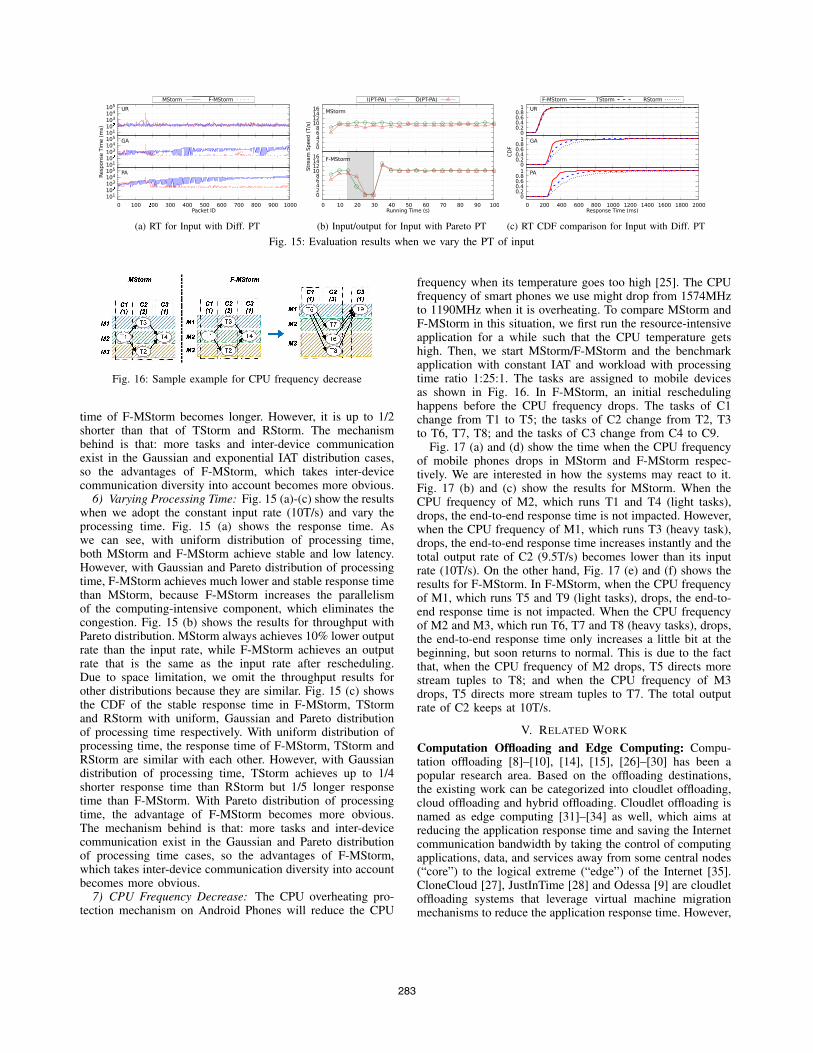
(a) RT for Input with Diff. PT (b) Input/output for Input with Pareto PT (c) RT CDF comparison for Input with Diff. PT

Fig. 15: Evaluation results when we vary the PT of input

Fig. 16: Sample example for CPU frequency decrease

time of F-MStorm becomes longer. However, it is up to 1/2shorter than that of TStorm and RStorm. The mechanismbehind is that: more tasks and inter-device communicationexist in the Gaussian and exponential IAT distribution cases,so the advantages of F-MStorm, which takes inter-devicecommunication diversity into account becomes more obvious.

6) Varying Processing Time: Fig. 15 (a)-(c) show the resultswhen we adopt the constant input rate (10T/s) and vary theprocessing time. Fig. 15 (a) shows the response time. Aswe can see, with uniform distribution of processing time,both MStorm and F-MStorm achieve stable and low latency.However, with Gaussian and Pareto distribution of processingtime, F-MStorm achieves much lower and stable response timethan MStorm, because F-MStorm increases the parallelismof the computing-intensive component, which eliminates thecongestion. Fig. 15 (b) shows the results for throughput withPareto distribution. MStorm always achieves 10% lower outputrate than the input rate, while F-MStorm achieves an outputrate that is the same as the input rate after rescheduling.Due to space limitation, we omit the throughput results forother distributions because they are similar. Fig. 15 (c) showsthe CDF of the stable response time in F-MStorm, TStormand RStorm with uniform, Gaussian and Pareto distributionof processing time respectively. With uniform distribution ofprocessing time, the response time of F-MStorm, TStorm andRStorm are similar with each other. However, with Gaussiandistribution of processing time, TStorm achieves up to 1/4shorter response time than RStorm but 1/5 longer responsetime than F-MStorm. With Pareto distribution of processingtime, the advantage of F-MStorm becomes more obvious.The mechanism behind is that: more tasks and inter-devicecommunication exist in the Gaussian and Pareto distributionof processing time cases, so the advantages of F-MStorm,which takes inter-device communication diversity into accountbecomes more obvious.

7) CPU Frequency Decrease: The CPU overheating pro-tection mechanism on Android Phones will reduce the CPU

frequency when its temperature goes too high [25]. The CPUfrequency of smart phones we use might drop from 1574MHzto 1190MHz when it is overheating. To compare MStorm andF-MStorm in this situation, we first run the resource-intensiveapplication for a while such that the CPU temperature getshigh. Then, we start MStorm/F-MStorm and the benchmarkapplication with constant IAT and workload with processingtime ratio 1:25:1. The tasks are assigned to mobile devicesas shown in Fig. 16. In F-MStorm, an initial reschedulinghappens before the CPU frequency drops. The tasks of C1change from T1 to T5; the tasks of C2 change from T2, T3to T6, T7, T8; and the tasks of C3 change from C4 to C9.

Fig. 17 (a) and (d) show the time when the CPU frequencyof mobile phones drops in MStorm and F-MStorm respec-tively. We are interested in how the systems may react to it.Fig. 17 (b) and (c) show the results for MStorm. When theCPU frequency of M2, which runs T1 and T4 (light tasks),drops, the end-to-end response time is not impacted. However,when the CPU frequency of M1, which runs T3 (heavy task),drops, the end-to-end response time increases instantly and thetotal output rate of C2 (9.5T/s) becomes lower than its inputrate (10T/s). On the other hand, Fig. 17 (e) and (f) shows theresults for F-MStorm. In F-MStorm, when the CPU frequencyof M1, which runs T5 and T9 (light tasks), drops, the end-to-end response time is not impacted. When the CPU frequencyof M2 and M3, which run T6, T7 and T8 (heavy tasks), drops,the end-to-end response time only increases a little bit at thebeginning, but soon returns to normal. This is due to the factthat, when the CPU frequency of M2 drops, T5 directs morestream tuples to T8; and when the CPU frequency of M3drops, T5 directs more stream tuples to T7. The total outputrate of C2 keeps at 10T/s.

V. RELATED WORK

Computation Offloading and Edge Computing: Compu-tation offloading [8]–[10], [14], [15], [26]–[30] has been apopular research area. Based on the offloading destinations,the existing work can be categorized into cloudlet offloading,cloud offloading and hybrid offloading. Cloudlet offloading isnamed as edge computing [31]–[34] as well, which aims atreducing the application response time and saving the Internetcommunication bandwidth by taking the control of computingapplications, data, and services away from some central nodes(“core”) to the logical extreme (“edge”) of the Internet [35].CloneCloud [27], JustInTime [28] and Odessa [9] are cloudletoffloading systems that leverage virtual machine migrationmechanisms to reduce the application response time. However,

283

0

300

600

900

1200

1500

1800

0 15 30 45 60 75 90 105 120 135 150

Fre

quen

cy (

MH

z)

Running Time (s)

M1 M2 M3

(a) CPU Freq. ↓ in MStorm

100

101

102

103

104

105

0 150 300 450 600 750 900 1050 1200 1350 1500

M2’s frequency decreases

M1’s frequency decreases

Res

pons

e T

ime

(ms)

Packet ID

MStorm

(b) RT with CPU Freq. ↓ in MStorm

0 1 2 3 4 5 6 7 8 9

10

0 20 40 60 80 100 120 140 160 180 200

Out

put (

T/s

)

Running Time (s)

T2(C2) at M3 T3(C2) at M1

(c) C2’s Output with CPU Freq. ↓ in MStorm

0

300

600

900

1200

1500

1800

0 15 30 45 60 75 90 105 120

Fre

quen

cy (

MH

z)

Running Time (s)

M1 M2 M3

(d) CPU Freq. ↓ in F-MStorm

100

101

102

103

104

105

0 100 200 300 400 500 600 700 800 900 1000

reschedule

M1’ frequency decreases

M2’ frequency decreases

M3’ frequency decreases

Res

pons

e T

ime

(ms)

Packet ID

F−MStorm

(e) RT with CPU Freq. ↓ in F-MStorm

0 1 2 3 4 5 6 7 8 9

10

0 10 20 30 40 50 60 70 80 90 100 110 120

Out

put (

T/s

)

Running Time (s)

T2(C2) at M3 T3(C2) at M1 T7(C2) at M2

T6(C2) at M3 T8(C2) at M3

(f) C2’s Output with CPU Freq. ↓ in F-MStorm

Fig. 17: How MStorm and F-MStorm deal with CPU frequency decrease

all these systems rely on powerful nearby cloudlets, which arenot always available in some critical scenarios like militaryoperations and disaster response, because soldiers or firstresponders have to move from place to place and they are onlyallowed to carry on some lightweight mobile devices. Differentfrom the above systems, F-MStorm only utilizes nearby mobiledevices as offloading destinations, which is more practical forthe military and disaster response scenarios, because soldiersand first responders always work together as a group andtheir mobile devices can be connected together as a cluster.MAUI [26] is a cloud offloading system which enables energy-aware offloading by using remote function calls to the cloud.MCDNN [8] is a cloud offloading framework that employsa runtime scheduler to trade off the application accuracyfor resource usage and latency. Orbit [30] and LEO [10]are similar systems that utilize profile-based partitioning ofapplications to offload computation tasks to hybrid computingresources. All these systems rely on the Internet access, whichhowever are not always available in some critical scenarios,because soldiers and first responders always work in someextremely difficult environments that do not provide any accessto the Internet. Different from these systems, F-MStorm doesnot rely on the Internet. Instead, it only needs a mobile deviceto be set up as a hotspot, such that all the mobile devicesin a group can be connected together. Some existing worklike Hyrax [14] and Serendipity [15] also offload computingtasks to the nearby mobile devices. However, their workfocuses on processing bounded batch jobs that have relativelylow requirements on the latency. Instead, F-MStorm focuseson processing unbounded stream data, which has a higherrequirement on the latency.

Distributed Stream Processing System: Apache Storm [11]is a distributed stream processing system deployed on cloudservers. Many improvements based on Storm have been pro-posed [19], [20], [36]–[39]. Among them, AdaptiveStorm [36]continuously monitors the system performance and resched-ules tasks at run-time to reduce the overall response time.T-Storm [19] accelerates stream processing by using traffic-aware scheduling, which minimizes the inter-device and inter-process traffics. R-Storm [20] improves the throughput andminimizes the network latency by maximizing the resource

utilization. All these works are closely related to F-MStorm,but they do not consider the detailed differences amonginter-device links, which however are essential in streamprocessing at the edge. The authors in [37] propose a scalablecentralized scheme for job reconfiguration, which minimizesthe communication cost while keeping the nodes below acomputational load threshold. The authors in [38] propose adynamic resource scheduler for cloud-based distributed streamprocessing systems, which measures the system workloadwith the minimal overhead and provisions the minimumresources to meet the response time constraints. The authorsin [39] provide a general formulation for the optimal datastream processing placement and takes explicitly into accountthe heterogeneity of computing and networking resources.Similar to these works, in F-MStorm, we propose a gen-eral framework for stream task assignment that takes delay,energy and load balance all into account. The difference isthat, our problem is more challenging, because in streamprocessing at the edge, the inter-device delay is dynamicand the users’ own application may cause disturbance to F-MStorm. Except for Storm and its subsequent improvements,there are other popular stream processing systems like ApacheSpark Stream [12], Flink [13], Samza [40], etc. However,all these systems are designed and implemented to run oncloud servers instead of mobile devices. To the best of ourknowledge, MStorm [1] is the first work that performs onlinedistributed mobile stream processing at the edge. However, itis inefficient in the system configuration, task scheduling andexecution aspects. F-MStorm improves its efficiency by usingthe feedback information.

VI. CONCLUSION AND FUTURE WORK

In this paper, we present a feedback-based online distributedmobile stream processing system running at the edge called F-MStorm. F-MStorm adopts feedback-based approach at manysystem design levels including configuration, scheduling andexecution. We implement F-MStorm on a cluster of Androidphones and evaluate its performance through extensive experi-ments. The experimental results show that F-MStorm achievesup to 3x shorter response time, 10% higher throughput and23% less energy consumption than the state-of-the-art mobilestream processing systems. It should be noted that, currently,

284

we only focus on the CPU bounded applications and assumeall mobile devices to be homogeneous in hardware. Wealso assume that the users in a group always stay in thewireless range of each other. In the future, we will consider aheterogeneous computing environment, take into account otherresource constraints like memory usage or network bandwidthand deal with the node failure case.

ACKNOWLEDGMENT

This material is based upon work supported by NationalInstitute of Standards and Technology (NIST) under Grant NO.(#70NANB17H190). We also appreciate the suggestions fromthe reviewers and our shepherd Dr. Eyal de Lara.

REFERENCES

[1] Q. Ning, C.-A. Chen, R. Stoleru, and C. Chen, “Mobile storm:Distributed real-time stream processing for mobile clouds,” in CloudNet’15. IEEE, pp. 139–145.

[2] D. M. Chen, S. S. Tsai, R. Vedantham, R. Grzeszczuk, and B. Girod,“Streaming mobile augmented reality on mobile phones,” in ISMAR ’09.IEEE, pp. 181–182.

[3] H. Lu, D. Frauendorfer, M. Rabbi, M. S. Mast, G. T. Chittaranjan, A. T.Campbell, D. Gatica-Perez, and T. Choudhury, “Stresssense: Detectingstress in unconstrained acoustic environments using smartphones,” inUbiComp ’12. ACM, pp. 351–360.

[4] Y. Lee, C. Min, C. Hwang, J. Lee, I. Hwang, Y. Ju, C. Yoo, M. Moon,U. Lee, and J. Song, “Sociophone: Everyday face-to-face interactionmonitoring platform using multi-phone sensor fusion,” in Moibsys ’13.ACM, pp. 375–388.

[5] G. Chen, C. Parada, and G. Heigold, “Small-footprint keyword spottingusing deep neural networks,” in ICASSP ’14. IEEE, pp. 4087–4091.

[6] N. D. Lane, P. Georgiev, and L. Qendro, “Deepear: Robust smartphoneaudio sensing in unconstrained acoustic environments using deeplearning,” in UbiComp ’15, pp. 283–294.

[7] I. Damian, C. S. S. Tan, T. Baur, J. Schoning, K. Luyten, and E. Andre,“Augmenting social interactions: Realtime behavioural feedback usingsocial signal processing techniques,” in CHI ’15, 2015, pp. 565–574.

[8] S. Han, H. Shen, M. Philipose, S. Agarwal, A. Wolman, and A. Krishna-murthy, “Mcdnn: An approximation-based execution framework for deepstream processing under resource constraints,” in Mobisys ’16. ACM,pp. 123–136.

[9] M.-R. Ra, A. Sheth, L. Mummert, P. Pillai, D. Wetherall, andR. Govindan, “Odessa: enabling interactive perception applications onmobile devices,” in Mobisys ’11. ACM, pp. 43–56.

[10] P. Georgiev, N. D. Lane, K. K. Rachuri, and C. Mascolo, “Leo:scheduling sensor inference algorithms across heterogeneous mobileprocessors and network resources,” in Mobicom ’16, pp. 320–333.

[11] A. Toshniwal, S. Taneja, A. Shukla, K. Ramasamy, J. M. Patel,S. Kulkarni, J. Jackson, K. Gade, M. Fu, J. Donham et al., “Storm@twitter,” in SIGMOD ’14. ACM, pp. 147–156.

[12] M. Zaharia, T. Das, H. Li, S. Shenker, and I. Stoica, “Discretizedstreams: An efficient and fault-tolerant model for stream processing onlarge clusters.” HotCloud ’12, vol. 12, pp. 10–10.

[13] P. Carbone, A. Katsifodimos, S. Ewen, V. Markl, S. Haridi, andK. Tzoumas, “Apache flink: Stream and batch processing in a singleengine,” Bulletin of the IEEE Computer Society Technical Committeeon Data Engineering, vol. 36, no. 4, 2015.

[14] E. E. Marinelli, “Hyrax: cloud computing on mobile devices usingmapreduce,” DTIC Document, Tech. Rep., 2009.

[15] C. Shi, V. Lakafosis, M. H. Ammar, and E. W. Zegura, “Serendipity:enabling remote computing among intermittently connected mobiledevices,” in Mobihoc ’12. ACM, pp. 145–154.

[16] J. Tang and T. Q. Quek, “The role of cloud computing in content-centricmobile networking,” IEEE Communications Magazine, vol. 54, no. 8,pp. 52–59, 2016.

[17] J. Dean and S. Ghemawat, “Mapreduce: a flexible data processing tool,”Communications of the ACM, vol. 53, no. 1, pp. 72–77, 2010.

[18] S. Venkataraman, A. Panda, K. Ousterhout, M. Armbrust, A. Ghodsi,M. J. Franklin, B. Recht, and I. Stoica, “Drizzle: Fast and adaptablestream processing at scale,” in Proceedings of the 26th Symposium onOperating Systems Principles. ACM, 2017, pp. 374–389.

[19] J. Xu, Z. Chen, J. Tang, and S. Su, “T-storm: Traffic-aware onlinescheduling in storm,” in ICDCS ’14. IEEE, pp. 535–544.

[20] B. Peng, M. Hosseini, Z. Hong, R. Farivar, and R. Campbell, “R-storm:Resource-aware scheduling in storm,” in Middleware ’15, pp. 149–161.

[21] L. Sun, R. K. Sheshadri, W. Zheng, and D. Koutsonikolas, “Modelingwifi active power/energy consumption in smartphones,” in ICDCS ’14.IEEE, pp. 41–51.

[22] “Network-Connection,” https://github.com/facebook/network-connection-class, 2016, [Online; accessed 14-Dec-2016].

[23] “API: CPLEX,” https://www.ibm.com/, 2016, [Online; accessed 14-Dec-2016].

[24] K. Deb, A. Pratap, S. Agarwal, and T. Meyarivan, “A fast andelitist multiobjective genetic algorithm: Nsga-ii,” IEEE transactions onevolutionary computation, vol. 6, no. 2, pp. 182–197, 2002.

[25] G. P. Srinivasa, R. Begum, S. Haseley, M. Hempstead, and G. Challen,“Separated by birth: Hidden differences between seemingly-identicalsmartphone cpus,” in HotMobile ’17. ACM, pp. 103–108.

[26] E. Cuervo, A. Balasubramanian, D.-k. Cho, A. Wolman, S. Saroiu,R. Chandra, and P. Bahl, “Maui: Making smartphones last longer withcode offload,” in MobiSys ’10. ACM, pp. 49–62.

[27] B.-G. Chun, S. Ihm, P. Maniatis, M. Naik, and A. Patti, “Clonecloud:elastic execution between mobile device and cloud,” in Proceedings ofthe sixth conference on Computer systems. ACM, 2011, pp. 301–314.

[28] K. Ha, P. Pillai, W. Richter, Y. Abe, and M. Satyanarayanan, “Just-in-time provisioning for cyber foraging,” in MobiSys ’13, pp. 153–166.

[29] P. Georgiev, N. D. Lane, K. K. Rachuri, and C. Mascolo, “Dsp.ear: Leveraging co-processor support for continuous audio sensing onsmartphones,” in SenSys ’14. ACM, pp. 295–309.

[30] M.-M. Moazzami, D. E. Phillips, R. Tan, and G. Xing, “Orbit:a smartphone-based platform for data-intensive embedded sensingapplications,” in IPSN ’15. ACM, pp. 83–94.

[31] M. Satyanarayanan, “The emergence of edge computing,” Computer,vol. 50, no. 1, pp. 30–39, 2017.

[32] K. Ha, Y. Abe, T. Eiszler, Z. Chen, W. Hu, B. Amos, R. Upadhyaya,P. Pillai, and M. Satyanarayanan, “You can teach elephants to dance:agile vm handoff for edge computing,” in SEC ’17. ACM, p. 12.

[33] L. Chaufournier, P. Sharma, F. Le, E. Nahum, P. Shenoy, and D. Towsley,“Fast transparent virtual machine migration in distributed edge clouds,”in SEC ’17. ACM, 2017, p. 10.

[34] Z. Chen, W. Hu, J. Wang, S. Zhao, B. Amos, G. Wu, K. Ha, K. Elgazzar,P. Pillai, R. Klatzky et al., “An empirical study of latency in anemerging class of edge computing applications for wearable cognitiveassistance,” in Proceedings of the Second ACM/IEEE Symposium onEdge Computing. ACM, 2017, p. 14.

[35] P. Garcia Lopez, A. Montresor, D. Epema, A. Datta, T. Higashino,A. Iamnitchi, M. Barcellos, P. Felber, and E. Riviere, “Edge-centric com-puting: Vision and challenges,” SIGCOMM Computer CommunicationReview, vol. 45, no. 5, pp. 37–42, 2015.

[36] L. Aniello, R. Baldoni, and L. Querzoni, “Adaptive online schedulingin storm,” in DEBS ’13. ACM, pp. 207–218.

[37] A. Chatzistergiou and S. D. Viglas, “Fast heuristics for near-optimaltask allocation in data stream processing over clusters,” in CIKM ’14.ACM, pp. 1579–1588.

[38] T. Z. Fu, J. Ding, R. T. Ma, M. Winslett, Y. Yang, and Z. Zhang, “Drs:dynamic resource scheduling for real-time analytics over fast streams,”in ICDCS ’15. IEEE, pp. 411–420.

[39] V. Cardellini, V. Grassi, F. Lo Presti, and M. Nardelli, “Optimal operatorplacement for distributed stream processing applications,” in DEBS ’16.ACM, pp. 69–80.

[40] “Apache Samza,” https://samza.apache.org/, 2017, [Online; accessed 14-Dec-2017].

285