Lecture 4

Interest Rates

• Interest Rate Mechanics – M&B 6

• Real vs. Nominal Rates – M&B 8, M&I 4.1

• Loanable Funds Model – M&B 19, pp. 1-3

• Debtor-Creditor Redistribution – M&I 7.1

F11 10/2, rev 10/5

Present Value (PV)

$PV now invested for m years at interest rate i has Future Value (FV):

FV = PV (1 + i)m

Future payment of $FV to be paid in m yrs has PV:

E.g., FV = $100, i = 5% (.05), m = 1 yr:

PV = $100 / (1.05) = $95.24.

or, if m = 20 yr,

PV = $100 / (1.05)20 = $100 / 2.6533 = $37.69.

Need xy or ^ key on calculator to compute!

Note: nominal interest rate “i” is “R” in M&B, M&I.

mi)1(

FVPV

• implies that holding FV constant,

i PV , i PV , and, m PV , m PV .

• Also, effect of i on PV grows proportionately stronger with m:

PV/PV - i · m

– Examples:

m = 1 yr, i rises from 5% to 6%, i = +1%, FV = 100:

- i · m = - (+1%)(1yr) = -1%

(Actual PV/PV = (94.34 – 95.24)/95.24 = - .0094 = - 0.94%)

m = 20 yrs, i rises from 5% to 6%:

- i · m = - (+1%)(20YR) = -20%

(Actual PV/PV = (31.18 – 37.69)/37.69 = - .173 = - 17.3%)

‒ Leads to Interest Rate Risk when banks or thrifts lend long,

borrow short. (More later)

mi)1(

FVPV

i from FV / PV:

PV = FV / (1+i)m

(1+i)m = FV / PV,

1+i = (FV / PV)1/m , so

i = (FV / PV)1/m – 1

E.g., FV = $100, PV = $50, m = 10 yrs.,

i = (100 / 50)1/10 – 1

= 20.1 – 1 = 1.0718 – 1 = 0.0718 = 7.18%.

Note: 0.01% = one “Basis Point”.

Bonds

Face Value $F to be paid at maturity m

Coupons $C paid each year for m years.

(Assume annual for simplicity – most semiannual)

Bond Present Value (PVB)

i PVB , i PVB

(but m could have either effect because payments are being added)

miii )1(

FC

)1(

C

)1(

CPV

2B

Yield to Maturity (YTM)

= the value of i that gives back market price of bond,

holding C, F, m constant.

If

PVB = F, bond is “at par”, YTM = C / F

PVB > F, bond is “above par”, YTM < C / F

PVB < F, bond is “below par”, YTM > C / F

E.g.

F = $100, C = $4, PVB = $100 YTM = 4%

F = $100, C = $3, PVB = $110 YTM < 3%

F = $100, C = $6, PVB = $90 YTM > 6%

Bond Duration*

Effect of i on PVB again proportionally stronger, the longer its m.

However, now,

PVB/PVB - i · D,

where the bond’s Duration D equals the present-

value-weighted average maturity of its payments:

Generally,

D = m if C = 0,

D < m if C > 0,

D increases with m

* aka Macaulay Duration

B2PV/

)1(

F)(m)(C

)1(

(2)C

)1(

(1)C

miiiD

Consols (Perpetuities)

Pay $C / yr. forever

Exist in UK, conceptually important

(1+i) PVC = C + PVC ,

PVC = C / i

E.g., C = $100, i = 4% PVC = 100/.04 = $2500

C

2

32C

PV)1(

1

1

)1(1)1(

1

1

)1()1(1PV

ii

C

i

C

i

C

ii

C

i

C

i

C

i

C

Consol Duration

DC = 1 / i

E.g., i = 4% / yr DC = 1 / .04 = 25 yrs.

DC finite despite infinite final maturity!

PVC/PVC - i · DC as for bonds

Real vs. Nominal Interest Rates

i = nominal interest rate

on $-denominated loans, not indexed for

inflation.

r = real interest rate

on purchasing-power-denominated loans,

with payments indexed for inflation

Note: nominal interest rate i is “R” in M&B, M&I. “R” will also

be used for bank reserves, so “i” less ambiguous.

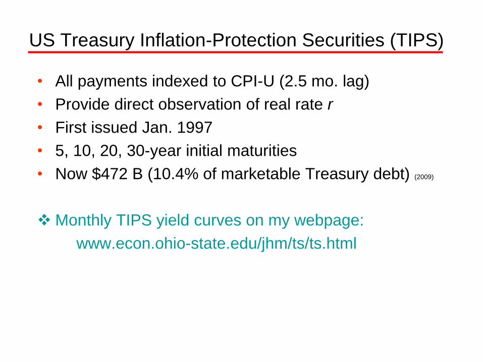
US Treasury Inflation-Protection Securities (TIPS)

• All payments indexed to CPI-U (2.5 mo. lag)

• Provide direct observation of real rate r

• First issued Jan. 1997

• 5, 10, 20, 30-year initial maturities

• Now $472 B (10.4% of marketable Treasury debt) (2009)

Monthly TIPS yield curves on my webpage:

www.econ.ohio-state.edu/jhm/ts/ts.html

Present Values with P-indexed loans

Same formulas, with r in place of i

PV = FV / (1+r)m, etc.

e.g. Indexed Consol:

C = Real coupon payment (today’s $)

PVC = C / r (today’s $)

application:

Parcel now pays $100,000 rent per year, future rent

assumed to grow in proportion to P. r = 2%.

PV = $100,000 / .02 = $5,000,000

• Real YTM r on 10-yr

TIPS has been between

0.5% and 4.5% since their

introduction in 1997.

Recent values under 0.5%

very unusual.

• Nominal YTM i on

conventional Treasuries

higher, to compensate for

likely future inflation. Also

more volatile, because of

fluctuations in inflation

premium.

i minus r gives “Break-

Even” inflation rate, at

which returns on real and

nominal bonds are equal.

According to the Fisher

Equation (next slide), this

is the market’s expectation

of future inflation e over

the life of the loans.

(thru Dec. 2008)

Determination of r, i

• Loanable Funds Model

real rate r primarily determined by savings, investment decisions, S and D for Credit.

• Fisher Equation

i = r + e, where e is expected inflation over life of loan

(sometimes written a for anticipated inflation)

• Adaptive Learning (AL) e mostly determined by past ,

with biggest weights on recent past.

Coefficients may change slowly over time.

-2

0

2

4

6

8

10

12

14

16

1950 1960 1970 1980 1990 2000 2010

Actual

Expected

Actual vs. Expected Inflation

Pe

rce

nt

pe

r a

nn

um

Actual year-over-year past inflation,

Adaptive Lag estimate of expected inflation for coming year

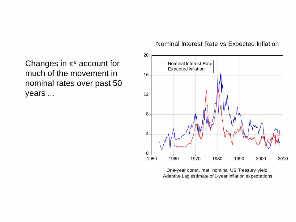
0

4

8

12

16

20

1950 1960 1970 1980 1990 2000 2010

Nominal Interest Rate

Expected Inflation

Nominal Interest Rate vs Expected Inflation

One-year const. mat. nominal US Treasury yield,

Adaptive Lag estimate of 1-year inflation expectations

Changes in e account for

much of the movement in

nominal rates over past 50

years ...

-6

-4

-2

0

2

4

6

8

1960 1970 1980 1990 2000 2010

Pe

rce

nt

pe

r a

nn

um

Inferred 1-Yr. US Real Interest Rate

1-year constant mat. nom. Treasury yield minus

Adaptive Lag est. of 1-year expected inflation

(1980 Carter

credit controls)

Early 80s Volcker

credit crunch

8/08

1970s

Burns-Miller

easy $

... but inferred real rates

have not been constant:

1-yr r typically about 2%,

but was 0-1% in 1970s,

5-6% in early 80s,

negative 2003-5, 2008-

2011 (not plotted).

Loanable Funds Model of r (M&I 19, pp. 1-3)

(1+r)m is price of present goods in terms of future goods

– r present goods more costly (rel. to future goods)

– r present goods less costly.

“Credit” = command over present goods

= what you get in exchange for your IOU when you borrow

= what you give up in exchange for someone else’s IOU when you lend.

Non-monetary equilibrium r determined by

Demand & Supply of Credit.

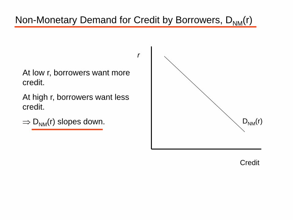
Credit

r

DNM(r)

At low r, borrowers want more

credit.

At high r, borrowers want less

credit.

DNM(r) slopes down.

Non-Monetary Demand for Credit by Borrowers, DNM(r)

Credit

r

SNM(r) At high r, lenders willing to give

up more credit

At low r, lenders give up less

credit.

SNM(r) slopes up

Non-Monetary Supply of Credit by Lenders

Credit

r

DNM(r)

SNM(r)

r0

Q0

Credit Market Equilibrium

(non-monetary economy)

r0 = Non-Monetary Equilibrium

real interest rate

Credit

r

DNM(r)

SNM(r)

r0

Q0

Credit Market Equilibrium

(non-monetary economy)

r0 = Non-Monetary Equilibrium

real interest rate

Increase in D for Credit

(rightward shift in DNM(r))

increases r0 to r0'

r0'

Credit

r

DNM(r)

SNM(r)

r0

Q0

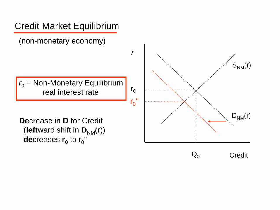
Credit Market Equilibrium

(non-monetary economy)

r0 = Non-Monetary Equilibrium

real interest rate

Decrease in D for Credit

(leftward shift in DNM(r))

decreases r0 to r0"

r0"

Credit

r

DNM(r)

SNM(r)

r0

Q0

Credit Market Equilibrium

(non-monetary economy)

r0 = Non-Monetary Equilibrium

real interest rate

Increase in S of Credit

(rightward shift in SNM(r))

DEcreases r0 to r0

(corrected 10/5/11)

r0'"

Credit

r

DNM(r)

SNM(r)

r0

Q0

Credit Market Equilibrium

(non-monetary economy)

r0 = Non-Monetary Equilibrium

real interest rate

Decrease in S of Credit

(leftward shift in SNM(r))

increases r0 to r0""

r0""

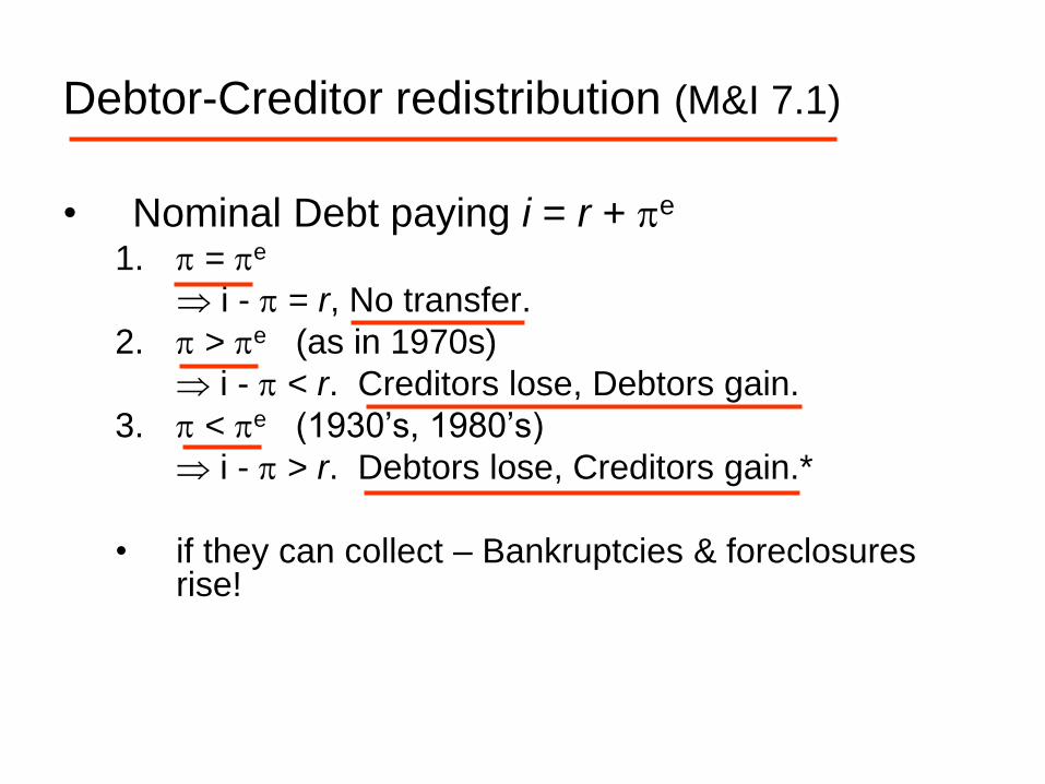
Debtor-Creditor redistribution (M&I 7.1)

• Nominal Debt paying i = r + e 1. = e

i - = r, No transfer.

2. > e (as in 1970s)

i - < r. Creditors lose, Debtors gain.

3. < e (1930’s, 1980’s)

i - > r. Debtors lose, Creditors gain.*

• if they can collect – Bankruptcies & foreclosures rise!

• Transfer may be eliminated with Price-Level

Indexed Debt.

– Payments indexed to CPI-U or other index

– Real return independent of inflation

– TIPS since 1997

• Nominal debt = safe indexed debt + lottery ticket

on CPI.

– Serves no function for risk-averse investors,

borrowers

– But still no private indexed securities to speak of!

• Next:

– Velocity and the Quantity Equation

• M&I 3, 4, 7.4

FOXTROT by Bill Amend